SDSU M. Vuskovic
MM-1
Real-Time
Audio and Video
NOTICE: This chapter is a prerequisite for the next chapter: Multimedia over IP
SDSU M. Vuskovic
MM-2
Multimedia Payloads
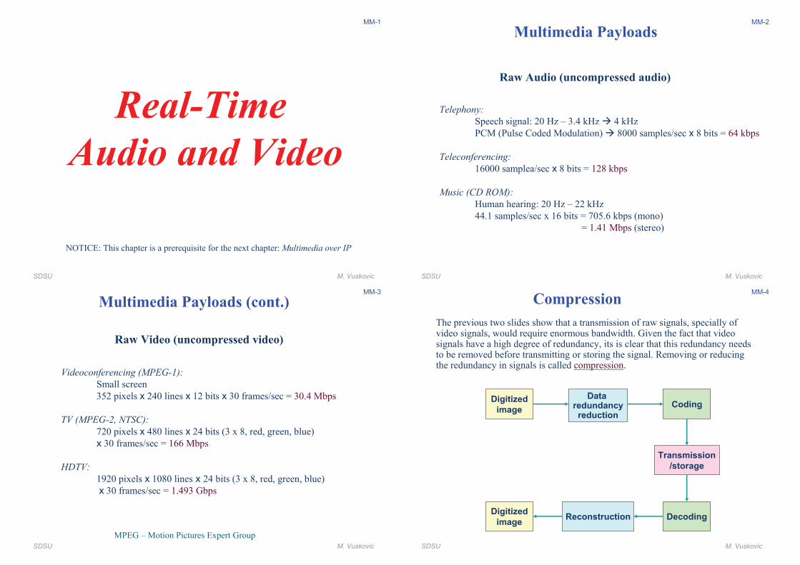
Raw Audio (uncompressed audio)
Telephony:
Speech signal: 20 Hz � 3.4 kHz ! 4 kHz
PCM (Pulse Coded Modulation) ! 8000 samples/sec x 8 bits = 64 kbps
Teleconferencing:
16000 samplea/sec x 8 bits = 128 kbps
Music (CD ROM):
Human hearing: 20 Hz � 22 kHz
44.1 samples/sec x 16 bits = 705.6 kbps (mono)
= 1.41 Mbps (stereo)
SDSU M. Vuskovic
MM-3
Raw Video (uncompressed video)
Videoconferencing (MPEG-1):
Small screen
352 pixels x 240 lines x 12 bits x 30 frames/sec = 30.4 Mbps
TV (MPEG-2, NTSC):
720 pixels x 480 lines x 24 bits (3 x 8, red, green, blue)
x 30 frames/sec = 166 Mbps
HDTV:
1920 pixels x 1080 lines x 24 bits (3 x 8, red, green, blue)
x 30 frames/sec = 1.493 Gbps
MPEG � Motion Pictures Expert Group
Multimedia Payloads (cont.)
SDSU M. Vuskovic
MM-4
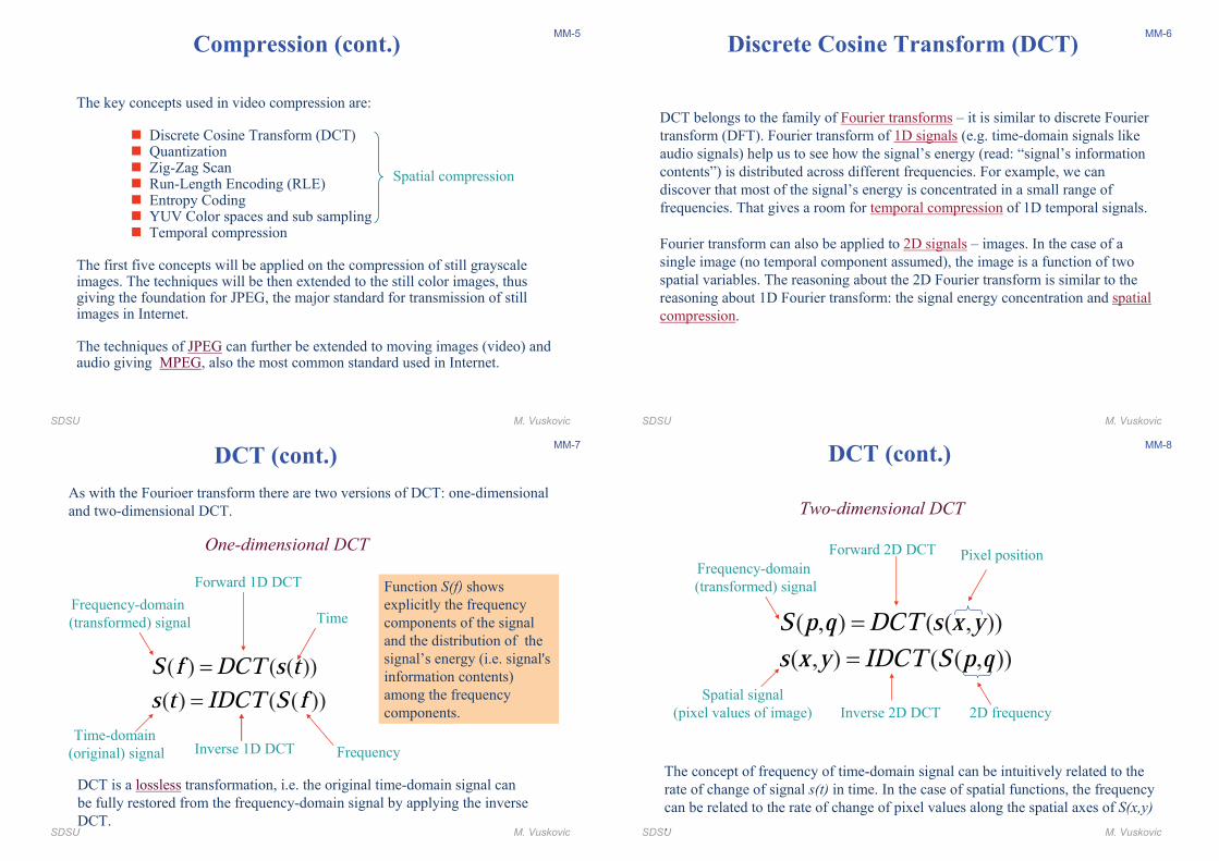
Digitized
image
Dataredundancyreduction
Coding
Transmission
/storage
DecodingReconstructionDigitized
image
Compression
The previous two slides show that a transmission of raw signals, specially of video signals, would require enormous bandwidth. Given the fact that video signals have a high degree of redundancy, its is clear that this redundancy needs to be removed before transmitting or storing the signal. Removing or reducing the redundancy in signals is called compression.
SDSU M. Vuskovic
MM-5
The key concepts used in video compression are:
" Discrete Cosine Transform (DCT)" Quantization" Zig-Zag Scan" Run-Length Encoding (RLE)" Entropy Coding" YUV Color spaces and sub sampling" Temporal compression
The first five concepts will be applied on the compression of still grayscale images. The techniques will be then extended to the still color images, thus giving the foundation for JPEG, the major standard for transmission of still images in Internet.
The techniques of JPEG can further be extended to moving images (video) and audio giving MPEG, also the most common standard used in Internet.
Compression (cont.)
Spatial compression
SDSU M. Vuskovic
MM-6
DCT belongs to the family of Fourier transforms � it is similar to discrete Fourier
transform (DFT). Fourier transform of 1D signals (e.g. time-domain signals like
audio signals) help us to see how the signal�s energy (read: �signal�s information
contents�) is distributed across different frequencies. For example, we can
discover that most of the signal�s energy is concentrated in a small range of
frequencies. That gives a room for temporal compression of 1D temporal signals.
Fourier transform can also be applied to 2D signals � images. In the case of a
single image (no temporal component assumed), the image is a function of two
spatial variables. The reasoning about the 2D Fourier transform is similar to the
reasoning about 1D Fourier transform: the signal energy concentration and spatial
compression.
Discrete Cosine Transform (DCT)
SDSU M. Vuskovic
MM-7
As with the Fourioer transform there are two versions of DCT: one-dimensional
and two-dimensional DCT.
DCT (cont.)
DCT is a lossless transformation, i.e. the original time-domain signal can
be fully restored from the frequency-domain signal by applying the inverse
DCT.
( ) ( ( ))
( ) ( ( ))
S f DCT s ts t IDCT S f
=
=
Frequency-domain
(transformed) signal
Time-domain
(original) signal Inverse 1D DCT
Forward 1D DCT
Time
Frequency
Function S(f) shows
explicitly the frequency
components of the signal
and the distribution of the
signal�s energy (i.e. signal's
information contents)
among the frequency
components.
One-dimensional DCT
SDSU M. Vuskovic
MM-8
DCT (cont.)
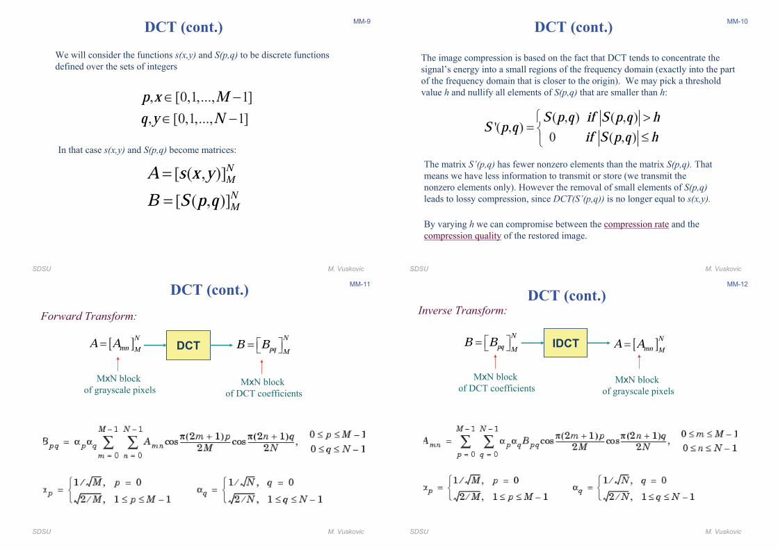
The concept of frequency of time-domain signal can be intuitively related to the
rate of change of signal s(t) in time. In the case of spatial functions, the frequency
can be related to the rate of change of pixel values along the spatial axes of S(x,y)
.
Frequency-domain
(transformed) signal
Spatial signal
(pixel values of image) Inverse 2D DCT
Forward 2D DCT Pixel position
2D frequency
( , ) ( ( , ))
( , ) ( ( , ))
S p q DCT s x ys x y IDCT S p q
=
=
Two-dimensional DCT
SDSU M. Vuskovic
MM-9
We will consider the functions s(x,y) and S(p,q) to be discrete functions
defined over the sets of integers
DCT (cont.)
, [0,1,..., 1]
, [0,1,..., 1]
p x Mq y N
∈ −
∈ −
In that case s(x,y) and S(p,q) become matrices:
[ ( , )]
[ ( , )]
NMNM
A s x yB S p q
=
=
SDSU M. Vuskovic
MM-10
DCT (cont.)
By varying h we can compromise between the compression rate and the
compression quality of the restored image.
The image compression is based on the fact that DCT tends to concentrate the
signal�s energy into a small regions of the frequency domain (exactly into the part
of the frequency domain that is closer to the origin). We may pick a threshold
value h and nullify all elements of S(p,q) that are smaller than h:
( , ) ( , )'( , )
0 ( , )
S p q if S p q hS p q if S p q h! >
= "≤#
The matrix S’(p,q) has fewer nonzero elements than the matrix S(p,q). That
means we have less information to transmit or store (we transmit the
nonzero elements only). However the removal of small elements of S(p,q)
leads to lossy compression, since DCT(S’(p,q)) is no longer equal to s(x,y).
SDSU M. Vuskovic
MM-11
DCT[ ]N
mn MA A=N
pq MB B$ %= & '
MxN block
of grayscale pixelsMxN block
of DCT coefficients
DCT (cont.)
Forward Transform:
SDSU M. Vuskovic
MM-12
IDCT [ ]N
mn MA A=N
pq MB B$ %= & '
MxN block
of grayscale pixels
MxN block
of DCT coefficients
DCT (cont.)Inverse Transform:
SDSU M. Vuskovic
MM-13
DCT[ ]N
mn MA A=
Npq MB B$ %= & '
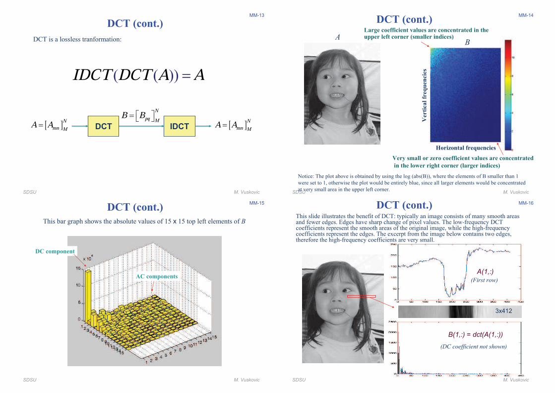
DCT (cont.)
DCT is a lossless tranformation:
( ( ))IDCT DCT A A=
IDCT [ ]N
mn MA A=
SDSU M. Vuskovic
MM-14
DCT (cont.)
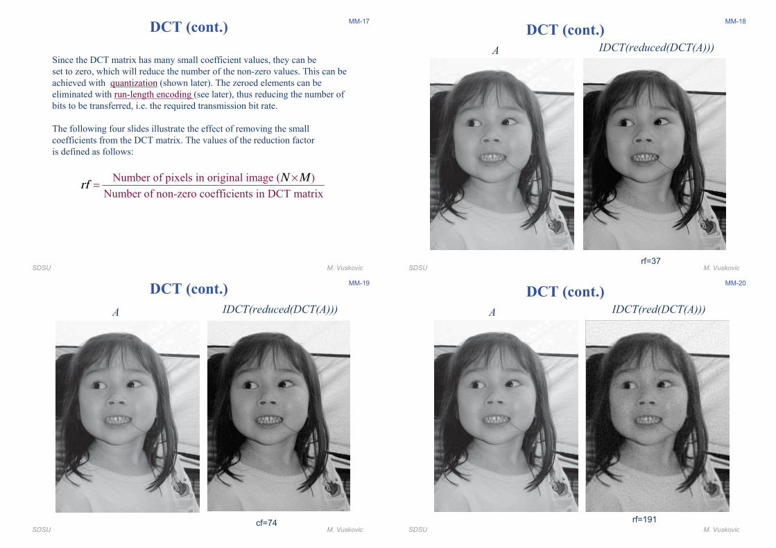
AB
Large coefficient values are concentrated in the upper left corner (smaller indices)
Very small or zero coefficient values are concentrated
in the lower right corner (larger indices)
Notice: The plot above is obtained by using the log (abs(B)), where the elements of B smaller than 1
were set to 1, otherwise the plot would be entirely blue, since all larger elements would be concentrated
at very small area in the upper left corner.
Horizontal frequencies
Verti
cal
freq
uen
cie
s
SDSU M. Vuskovic
MM-15
DCT (cont.)
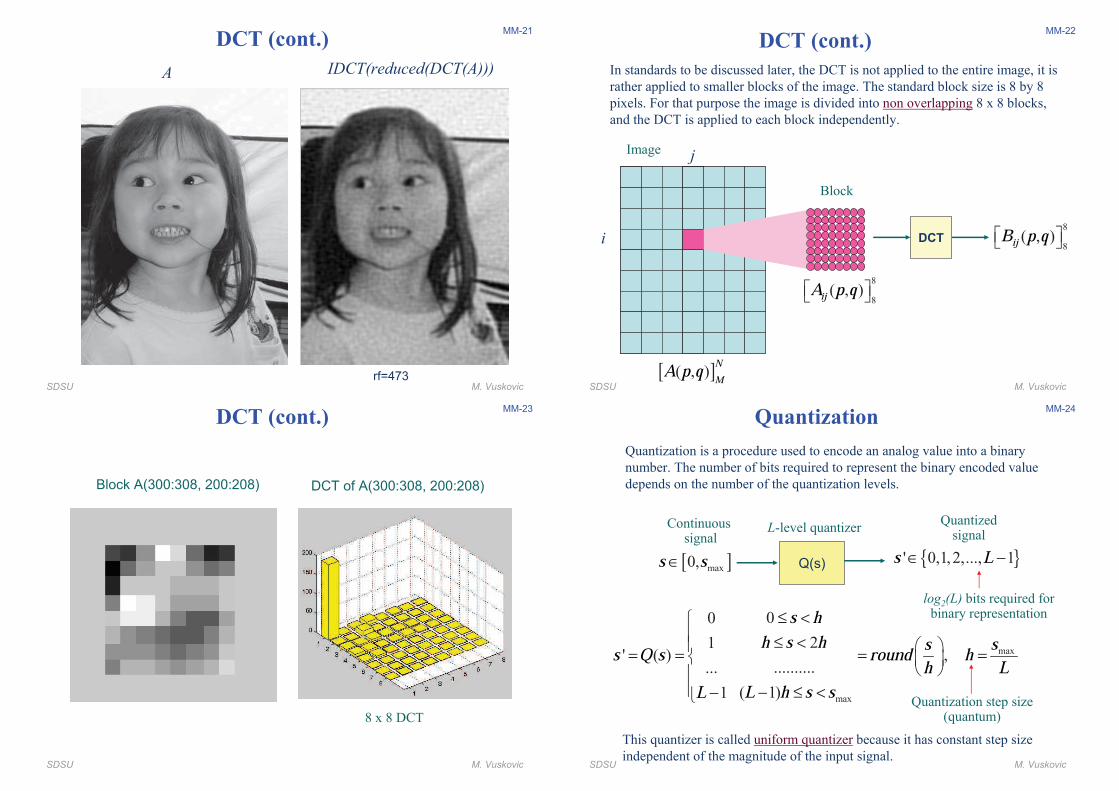
This bar graph shows the absolute values of 15 x 15 top left elements of B
DC component
AC components
SDSU M. Vuskovic
MM-16
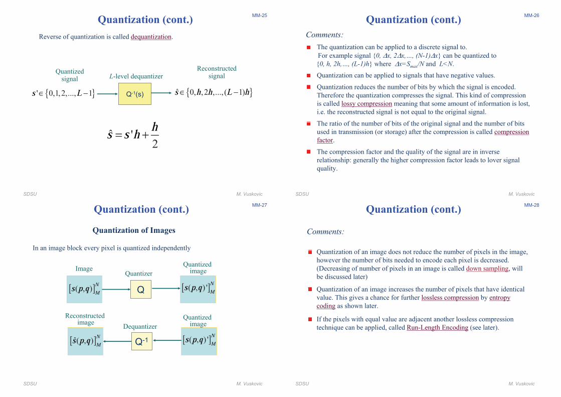
A(1,:)
B(1,:) = dct(A(1,:))
3x412
(DC coefficient not shown)
(First row)
DCT (cont.)This slide illustrates the benefit of DCT: typically an image consists of many smooth areas and fewer edges. Edges have sharp change of pixel values. The low-frequency DCT coefficients represent the smooth areas of the original image, while the high-frequency coefficients represent the edges. The excerpt from the image below contains two edges, therefore the high-frequency coefficients are very small.
SDSU M. Vuskovic
MM-17
DCT (cont.)
Since the DCT matrix has many small coefficient values, they can be
set to zero, which will reduce the number of the non-zero values. This can be
achieved with quantization (shown later). The zeroed elements can be
eliminated with run-length encoding (see later), thus reducing the number of
bits to be transferred, i.e. the required transmission bit rate.
The following four slides illustrate the effect of removing the small
coefficients from the DCT matrix. The values of the reduction factor
is defined as follows:
Number of pixels in original image ( )
Number of non-zero coefficients in DCT matrix
N Mrf ×=
SDSU M. Vuskovic
MM-18
rf=37
A
DCT (cont.)IDCT(reduced(DCT(A)))
SDSU M. Vuskovic
MM-19
cf=74
DCT (cont.)
IDCT(reduced(DCT(A)))A
SDSU M. Vuskovic
MM-20
rf=191
DCT (cont.)IDCT(red(DCT(A)))A
SDSU M. Vuskovic
MM-21
rf=473
DCT (cont.)
IDCT(reduced(DCT(A)))A
SDSU M. Vuskovic
MM-22
DCT (cont.)
In standards to be discussed later, the DCT is not applied to the entire image, it is
rather applied to smaller blocks of the image. The standard block size is 8 by 8
pixels. For that purpose the image is divided into non overlapping 8 x 8 blocks,
and the DCT is applied to each block independently.
Block
Image
DCT
8
8( , )ijA p q$ %& '
[ ]( , )NMA p q
8
8( , )ijB p q$ %& 'i
j
SDSU M. Vuskovic
MM-23
DCT (cont.)
Block A(300:308, 200:208) DCT of A(300:308, 200:208)
8 x 8 DCT
SDSU M. Vuskovic
MM-24
Quantization
Quantization is a procedure used to encode an analog value into a binary
number. The number of bits required to represent the binary encoded value
depends on the number of the quantization levels.
Q(s)[ ]max0,s s∈ { }' 0,1,2,..., 1∈ −s LContinuous
signal
Quantizedsignal
log2(L) bits required for binary representation
max
max
00
21' ( ) ,
.............
( 1)1
s hh s h sss Q s round hh L
L h s sL
≤ <!( ≤ <( ) *
= = = =" + ,- .(
( − ≤ <−#
L-level quantizer
Quantization step size(quantum)
This quantizer is called uniform quantizer because it has constant step size
independent of the magnitude of the input signal.
SDSU M. Vuskovic
MM-25
Quantization (cont.)
Reverse of quantization is called dequantization.
Q-1(s){ }' 0,1,2,..., 1∈ −s L
Quantizedsignal
Reconstructed signalL-level dequantizer
{ }� 0, ,2 ,..., ( 1)∈ −s h h L h
� '2
hs s h= +
SDSU M. Vuskovic
MM-26
Quantization (cont.)
Comments:
The quantization can be applied to a discrete signal to.
For example signal {0, ∆x, 2∆x,…, (N-1)∆x} can be quantized to
{0, h, 2h,…, (L-1)h} where ∆x=Smax/N and L<N.
Quantization can be applied to signals that have negative values.
Quantization reduces the number of bits by which the signal is encoded.
Therefore the quantization compresses the signal. This kind of compression
is called lossy compression meaning that some amount of information is lost,
i.e. the reconstructed signal is not equal to the original signal.
The ratio of the number of bits of the original signal and the number of bits
used in transmission (or storage) after the compression is called compression
factor.
The compression factor and the quality of the signal are in inverse
relationship: generally the higher compression factor leads to lover signal
quality.
SDSU M. Vuskovic
MM-27
Quantization (cont.)
Quantization of Images
In an image block every pixel is quantized independently
Q[ ]( , )NMs p q [ ]( , ) '
NMs p q
QuantizedimageImage
Q-1[ ]�( , )NMs p q [ ]( , ) '
NMs p q
Reconstructed image
Quantizer
Dequantizer
Quantizedimage
SDSU M. Vuskovic
MM-28
Quantization (cont.)
Comments:
Quantization of an image does not reduce the number of pixels in the image,
however the number of bits needed to encode each pixel is decreased.
(Decreasing of number of pixels in an image is called down sampling, will
be discussed later)
Quantization of an image increases the number of pixels that have identical
value. This gives a chance for further lossless compression by entropy
coding as shown later.
If the pixels with equal value are adjacent another lossless compression
technique can be applied, called Run-Length Encoding (see later).
SDSU M. Vuskovic
MM-29
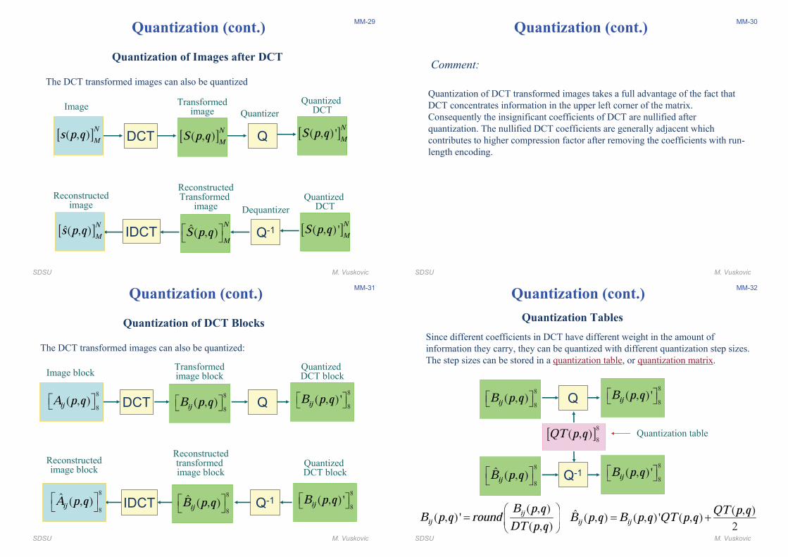
Quantization (cont.)
Quantization of Images after DCT
The DCT transformed images can also be quantized
[ ]( , ) 'NMS p q
QuantizedDCT
[ ]( , )NMs p q
Image
Q
Quantizer
DCT [ ]( , )NMS p q
Transformedimage
[ ]( , ) 'NMS p q
QuantizedDCT
[ ]�( , )NMs p q
Reconstructedimage
Q-1
Dequantizer
IDCT �( , )NM
S p q$ %& '
ReconstructedTransformed
image
SDSU M. Vuskovic
MM-30
Quantization (cont.)
Comment:
Quantization of DCT transformed images takes a full advantage of the fact that
DCT concentrates information in the upper left corner of the matrix.
Consequently the insignificant coefficients of DCT are nullified after
quantization. The nullified DCT coefficients are generally adjacent which
contributes to higher compression factor after removing the coefficients with run-
length encoding.
SDSU M. Vuskovic
MM-31
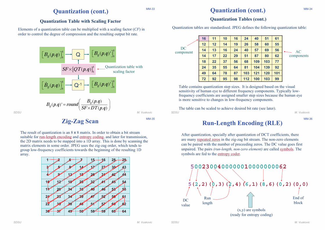
Quantization (cont.)
Quantization of DCT Blocks
The DCT transformed images can also be quantized:
QuantizedDCT blockImage block
Transformedimage block
8
8( , ) 'ijB p q$ %& '
8
8( , )ijA p q$ %& ' QDCT
8
8( , )ijB p q$ %& '
QuantizedDCT block
Reconstructedimage block
Reconstructedtransformed image block
8
8( , ) 'ijB p q$ %& '
8
8
� ( , )ijA p q$ %& ' Q-1IDCT
8
8
� ( , )ijB p q$ %& '
SDSU M. Vuskovic
MM-32
Quantization (cont.)
Quantization Tables
Since different coefficients in DCT have different weight in the amount of
information they carry, they can be quantized with different quantization step sizes.
The step sizes can be stored in a quantization table, or quantization matrix.
8
8( , ) 'ijB p q$ %& 'Q
8
8( , )ijB p q$ %& '
8
8( , ) 'ijB p q$ %& 'Q-1
8
8
� ( , )ijB p q$ %& '
( , )( , ) '
( , )
ijij
B p qB p q round DT p q) *
= + ,- .
( , )� ( , ) ( , ) ' ( , )2
ij ijQT p qB p q B p q QT p q= +
[ ]8
8( , )QT p q Quantization table
SDSU M. Vuskovic
MM-33
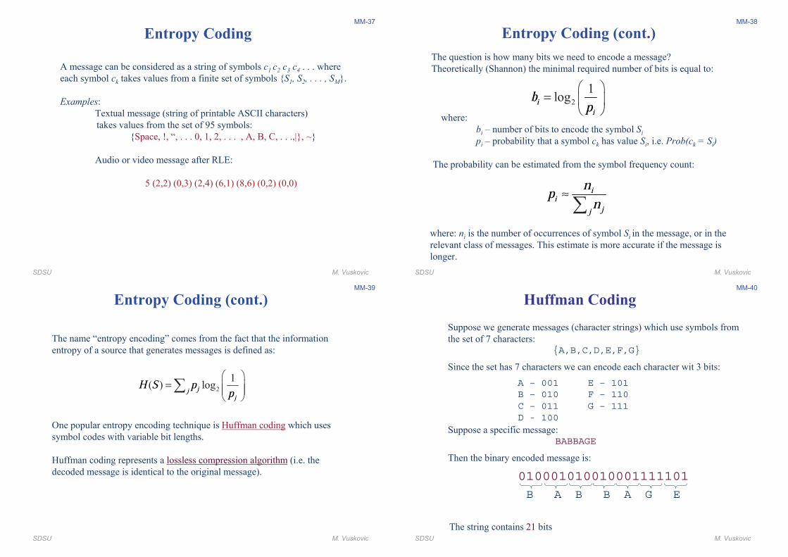
Quantization (cont.)
Quantization Table with Scaling Factor
Elements of a quantization table can be multiplied with a scaling factor (CF) in
order to control the degree of compression and the resulting output bit rate.
8
8( , ) 'ijB p q$ %& 'Q
8
8( , )ijB p q$ %& '
8
8( , ) 'ijB p q$ %& 'Q-1
8
8
� ( , )ijB p q$ %& '
( , )( , ) '
( , )
ijij
B p qB p q round SF DT p q) *
= + ,×- .
[ ]8
8( , )SF QT p q×
Quantization table with
scaling factor
SDSU M. Vuskovic
MM-34
6280875129221714
771031096856372218
921391048164553524
10112012110387786449
112
40
26
24
100
57
58
40
103
69
60
51
9998959272
5624161314
5519141212
6116101116
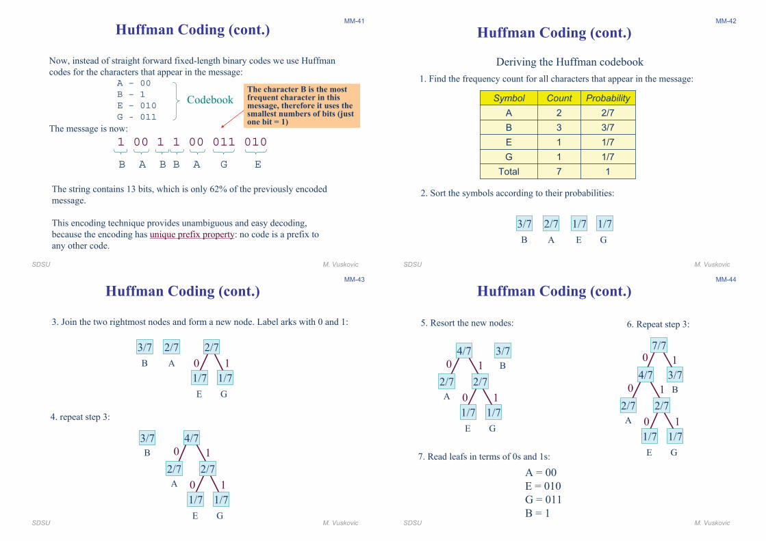
Quantization Tables (cont.)
Table contains quantization step sizes. It is designed based on the visual sensitivity of human eye to different frequency components. Typically low-frequency coefficients are assigned smaller step sizes because the human eye is more sensitive to changes in low-frequency components.
The table can be scaled to achieve desired bit rate (see later).
DC component AC
components
Quantization (cont.)
Quantization tables are standardised. JPEG defines the following quantization table:
SDSU M. Vuskovic
MM-35
Zig-Zag Scan
58
51
47
40
32
26
17
15
59
57
52
46
41
31
27
16
63
60
56
53
45
42
30
28
5425191210
5533242011
6139342321
6248383522
6450493736
44181394
4314853
297621
The result of quantization is an 8 x 8 matrix. In order to obtain a bit stream suitable for run-length encoding and entropy coding, and later for transmission, the 2D matrix needs to be mapped into a 1D array. This is done by scanning the matrix elements in some order. JPEG uses the zig-zag order, which tends to group low-frequency coefficients towards the beginning of the resulting 1Darray.
SDSU M. Vuskovic
MM-36
Run-Length Encoding (RLE)
After quantization, specially after quantization of DCT coefficients, there
are many repeated zeros in the zig-zag bit stream. The non-zero elements
can be paired with the number of preceeding zeros. The DC value goes first
unpaired. The pairs (run-length, non-zero element) are called symbols. The
symbols are fed to the entropy coder.
5002300400000010000000062
5(2,2)(0,3)(2,4)(6,1)(8,6)(0,2)(0,0)
Run
length
End of
block
(x,y) are symbols
(ready for entropy coding)
DC
value
SDSU M. Vuskovic
MM-37
A message can be considered as a string of symbols c1 c2 c3 c4 . . . where
each symbol ck takes values from a finite set of symbols {S1, S2, . . . , SM}.
Examples:
Textual message (string of printable ASCII characters)
takes values from the set of 95 symbols:
{Space, !, �, . . . 0, 1, 2, . . . , A, B, C, . . .,|}, ~}
Audio or video message after RLE:
5 (2,2) (0,3) (2,4) (6,1) (8,6) (0,2) (0,0)
Entropy Coding
SDSU M. Vuskovic
MM-38
The question is how many bits we need to encode a message?
Theoretically (Shannon) the minimal required number of bits is equal to:
Entropy Coding (cont.)
2
1logi
ib p
) *= + ,
- .where:
bi � number of bits to encode the symbol Si
pi � probability that a symbol ck has value Si, i.e. Prob(ck = Si)
The probability can be estimated from the symbol frequency count:
ii
jj
np n≈/
where: ni is the number of occurrences of symbol Si in the message, or in the
relevant class of messages. This estimate is more accurate if the message is
longer.
SDSU M. Vuskovic
MM-39
One popular entropy encoding technique is Huffman coding which uses
symbol codes with variable bit lengths.
Huffman coding represents a lossless compression algorithm (i.e. the
decoded message is identical to the original message).
Entropy Coding (cont.)
The name �entropy encoding� comes from the fact that the information
entropy of a source that generates messages is defined as:
2
1( ) logjj
jH S p p
) *= + ,+ ,
- ./
SDSU M. Vuskovic
MM-40
Huffman Coding
Suppose we generate messages (character strings) which use symbols from
the set of 7 characters:
{A,B,C,D,E,F,G}
Since the set has 7 characters we can encode each character wit 3 bits:
A – 001 E – 101B – 010 F – 110C – 011 G – 111D - 100
Suppose a specific message:
BABBAGE
Then the binary encoded message is:
010001010010001111101
B A B B A G E
The string contains 21 bits
SDSU M. Vuskovic
MM-41
Now, instead of straight forward fixed-length binary codes we use Huffman
codes for the characters that appear in the message:
A – 00B – 1E – 010G - 011
The message is now:
1 00 1 1 00 011 010
B A B B A G E
The string contains 13 bits, which is only 62% of the previously encoded
message.
This encoding technique provides unambiguous and easy decoding,
because the encoding has unique prefix property: no code is a prefix to
any other code.
Codebook
Huffman Coding (cont.)
The character B is the mostfrequent character in this message, therefore it uses the smallest numbers of bits (just one bit = 1)
SDSU M. Vuskovic
MM-42
Deriving the Huffman codebook
1. Find the frequency count for all characters that appear in the message:
7
1
1
3
2
Count
1/7G
1Total
1/7E
3/7B
2/7A
ProbabilitySymbol
2. Sort the symbols according to their probabilities:
3/7 2/7 1/7 1/7
B A E G
Huffman Coding (cont.)
SDSU M. Vuskovic
MM-43
3. Join the two rightmost nodes and form a new node. Label arks with 0 and 1:
3/7 2/7
B A
E G
1/7 1/7
2/7
0 1
4. repeat step 3:
3/7
B
A
E G
1/7 1/7
0 1
4/7
2/7 2/7
0 1
Huffman Coding (cont.)
SDSU M. Vuskovic
MM-44
5. Resort the new nodes: 6. Repeat step 3:
3/7
B
A
E G
1/7 1/7
0 1
4/7
2/7 2/7
0 1
A
E G
1/7 1/7
0 1
2/7 2/7
0 1
0 1
3/7
B
4/7
7/7
7. Read leafs in terms of 0s and 1s:
A = 00
E = 010
G = 011
B = 1
Huffman Coding (cont.)
SDSU M. Vuskovic
MM-45
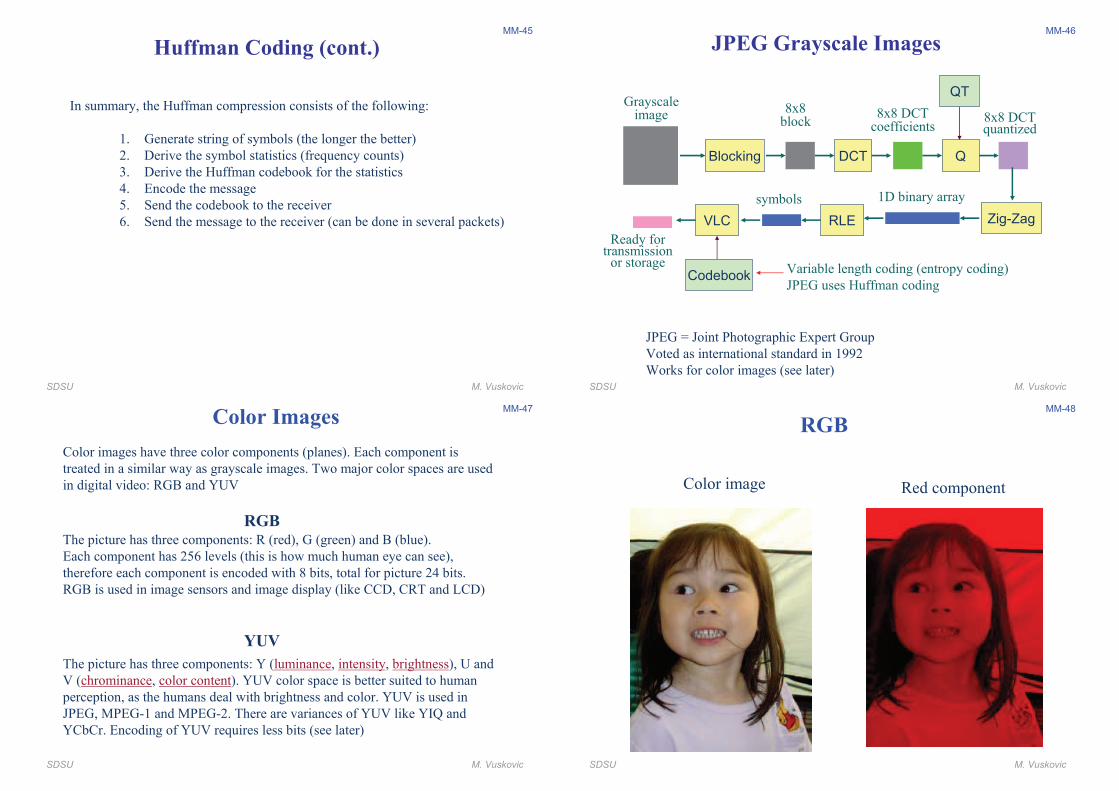
In summary, the Huffman compression consists of the following:
1. Generate string of symbols (the longer the better)
2. Derive the symbol statistics (frequency counts)
3. Derive the Huffman codebook for the statistics
4. Encode the message
5. Send the codebook to the receiver
6. Send the message to the receiver (can be done in several packets)
Huffman Coding (cont.)
SDSU M. Vuskovic
MM-46
JPEG Grayscale Images
Blocking DCT Q
Zig-ZagRLEVLC
8x8block
Grayscaleimage 8x8 DCT
coefficients8x8 DCTquantized
1D binary array
Codebook
QT
symbols
Ready fortransmission
or storage Variable length coding (entropy coding)
JPEG uses Huffman coding
JPEG = Joint Photographic Expert Group
Voted as international standard in 1992
Works for color images (see later)
SDSU M. Vuskovic
MM-47
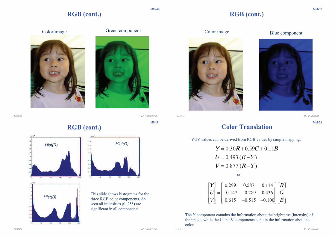
Color Images
RGBThe picture has three components: R (red), G (green) and B (blue).
Each component has 256 levels (this is how much human eye can see),
therefore each component is encoded with 8 bits, total for picture 24 bits.
RGB is used in image sensors and image display (like CCD, CRT and LCD)
YUV
The picture has three components: Y (luminance, intensity, brightness), U and
V (chrominance, color content). YUV color space is better suited to human
perception, as the humans deal with brightness and color. YUV is used in
JPEG, MPEG-1 and MPEG-2. There are variances of YUV like YIQ and
YCbCr. Encoding of YUV requires less bits (see later)
Color images have three color components (planes). Each component is
treated in a similar way as grayscale images. Two major color spaces are used
in digital video: RGB and YUV
SDSU M. Vuskovic
MM-48
RGB
Color image Red component
SDSU M. Vuskovic
MM-49
Green component
RGB (cont.)
Color image
SDSU M. Vuskovic
MM-50
Color image Blue component
RGB (cont.)
SDSU M. Vuskovic
MM-51
Hist(R) Hist(G)
Hist(B)
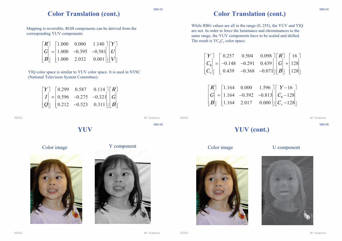
RGB (cont.)
This slide shows histograms for the
three RGB color components. As
seen all intensities (0..255) are
significant in all components.
SDSU M. Vuskovic
MM-52
Color Translation
or
0.30 0.59 0.11
0.493 ( )
0.877 ( )
Y R G BU B YV R Y
= + +
= −
= −
0.299 0.587 0.114
0.147 0.289 0.436
0.615 0.515 0.100
Y RU GV B
$ % $ % $ %0 1 0 1 0 1= − −0 1 0 1 0 1
− −0 1 0 1 0 1& ' & ' & '
YUV values can be derived from RGB values by simple mapping:
The Y component contains the information about the brightness (intensity) of
the image, while the U and V components contain the information abou the
color.
SDSU M. Vuskovic
MM-53
0.299 0.587 0.114
0.596 0.275 0.321
0.212 0.523 0.311
Y RI GQ B
$ % $ % $ %0 1 0 1 0 1= − −0 1 0 1 0 1
−0 1 0 1 0 1& ' & ' & '
1.000 0.000 1.140
1.000 0.395 0.581
1.000 2.032 0.001
R YG UB V
$ % $ % $ %0 1 0 1 0 1= − −0 1 0 1 0 10 1 0 1 0 1& ' & ' & '
Mapping is reversible, RGB components can be derived from the
corresponding YUV components:
YIQ color space is similar to YUV color space. It is used in NTSC
(National Television System Committee):
Color Translation (cont.)
SDSU M. Vuskovic
MM-54
While RBG values are all in the range (0..255), the YUV and YIQ
are not. In order to force the luminance and chrominances to the
same range, the YUV components have to be scaled and shifted.
The result is YCbCr color space:
0.257 0.504 0.098 16
0.148 0.291 0.439 128
0.439 0.368 0.071 128
b
r
Y RC GC B
$ % $ % $ % $ %0 1 0 1 0 1 0 1= − − +0 1 0 1 0 1 0 1
− −0 1 0 1 0 1 0 1& ' & ' & ' & '
1.164 0.000 1.596 16
1.164 0.392 0.813 128
1.164 2.017 0.000 128
b
r
R YG CB C
−$ % $ % $ %0 1 0 1 0 1= − − −0 1 0 1 0 1
−0 1 0 1 0 1& ' & ' & '
Color Translation (cont.)
SDSU M. Vuskovic
MM-55
YUV
Color image Y component
SDSU M. Vuskovic
MM-56
YUV (cont.)
Color image U component
SDSU M. Vuskovic
MM-57
YUV (cont.)
Color image V component
SDSU M. Vuskovic
MM-58
log(Hist(Y))log(Hist(U))
log(Hist(V))
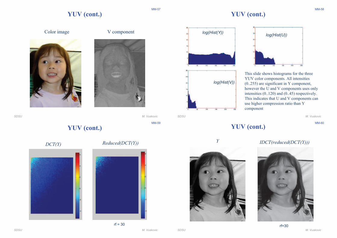
YUV (cont.)
This slide shows histograms for the three
YUV color components. All intensities
(0..255) are significant in Y component,
however the U and V components uses only
intensities (0..120) and (0..45) respectively.
This indicates that U and V components can
use higher compression ratio than Y
component
SDSU M. Vuskovic
MM-59
DCT(Y)
YUV (cont.)
rf = 30
Reduced(DCT(Y))
SDSU M. Vuskovic
MM-60
Y
rf=30
IDCT(reduced(DCT(Y)))
YUV (cont.)
SDSU M. Vuskovic
MM-61
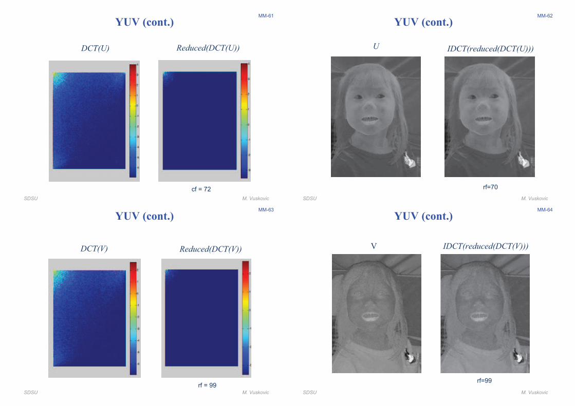
DCT(U)
cf = 72
YUV (cont.)
Reduced(DCT(U))
SDSU M. Vuskovic
MM-62
rf=70
U IDCT(reduced(DCT(U)))
YUV (cont.)
SDSU M. Vuskovic
MM-63
DCT(V)
rf = 99
Reduced(DCT(V))
YUV (cont.)
SDSU M. Vuskovic
MM-64
V
rf=99
IDCT(reduced(DCT(V)))
YUV (cont.)
SDSU M. Vuskovic
MM-65
99 10310011298959272
10112012110387786449
921131048164553524
771031096856372218
6280875129221714
5669574024161312
5560582619141212
6151402416101116
Luminance Quantization Table
(Y)
99 99 99 99 99 99 99 99
99 99 99 99 99 99 99 99
99 99 99 99 99 99 99 99
99 99 99 99 99 99 99 99
99 99 99 99 99 99 66 47
99 99 99 99 99 56 26 24
99 99 99 99 66 26 21 18
99 99 99 99 47 24 18 17
ChrominanceQuantization Table
(U,V/I,Q/Cb,Cr)
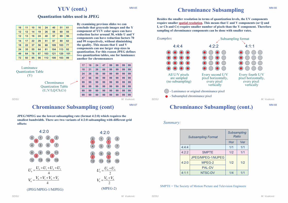
Quantization tables used in JPEG
YUV (cont.)
By examining previous slides we can conclude that grayscale images and the Y component of YUV color space can have reduction factor around 30, while U and V components can have reduction factors 70 and 99 respectively, without diminishing the quality. This means that U and V components can use larger step sizes in quantization. For this reason JPEG defines two quantization tables, one for luminance another for chromonances
SDSU M. Vuskovic
MM-66
All U/V pixels are sampled
(no subsampling)
Chrominance Subsampling
Besides the smaller resolution in terms of quantization levels, the UV components
require smaller spatial resolution. This means that U and V components (or Q and
I, or Cb and Cr) require smaller number of pixels than the Y component. Therefore
sampling of chrominance components can be done with smaller rates.
Examples:
4:4:4 4:2:2 4:1:1
Every second U/Vpixel horizontally,
every pixel vertically
Every fourth U/Vpixel horizontally,
every pixel vertically
- Luminance or original chrominance pixel
- Subsampled chrominance pixel
Subsampling format
SDSU M. Vuskovic
MM-67
Chrominance Subsampling (cont)
JPEG/MPEG use the lowest subsampling rate (format 4:2:0) which requires the
smallest bandwidth. There are two variants of 4:2:0 subsampling with different grid
offsets:
0 1 2 30
4 5 6 7
8 9 10 11
12 13 14 15
4:2:0
1
32
0 1 2 30
4 5 6 7
8 9 10 11
12 13 14 15
4:2:0
1
32
' 0 1 4 50
' 0 1 4 50
4
4
U U U UUV V V VV
+ + +=
+ + +=
' 0 40
' 0 40
2
2
U UUV VV
+=
+=
(JPEG/MPEG-1/MJPEG) (MPEG-2)
SDSU M. Vuskovic
MM-68
1/11/4NTSC-DV4:1:1
PAL-DV
MPEG-2 1/21/2
JPEG/MPEG-1/MJPEG
4:2:0
1/11/2SMPTE4:2:2
1/11/14:4:4
VerHor
Subsampling
RatioSubsampling Format
SMPTE = The Society of Motion Picture and Television Engineers
Chrominance Subsampling (cont.)
Summary:
SDSU M. Vuskovic
MM-69
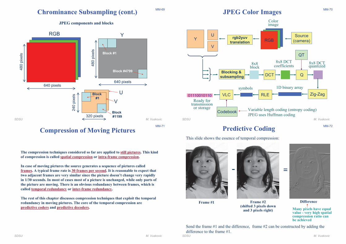
Chrominance Subsampling (cont.)
JPEG components and blocks480 p
ixels
RGB
640 pixels640 pixels
480 p
ixels
Y
320 pixels
240 p
ixels
Block #1
Block #4799
Block
#1
Block
#1199
V
U
SDSU M. Vuskovic
MM-70
JPEG Color Images
Q
Zig-ZagRLEVLC01110010110
8x8block
8x8 DCTcoefficients
8x8 DCTquantized
1D binary array
Codebook
QT
symbols
Ready fortransmission
or storage Variable length coding (entropy coding)
JPEG uses Huffman coding
RGB
Colorimage
YU
V
rgb2yuv
translation
Source
(camera)
DCTBlocking &
subsampling
SDSU M. Vuskovic
MM-71
Compression of Moving Pictures
The compression techniques considered so far are applied to still pictures. This kind
of compression is called spatial compression or intra-frame compression.
In case of moving pictures the source generates a sequence of pictures called
frames. A typical frame rate is 30 frames per second. It is reasonable to expect that
two adjacent frames are very similar since the picture doesn’t change very rapidly
in 1/30 seconds. In most of cases most of a picture is unchanged, while only parts of
the picture are moving. There is an obvious redundancy between frames, which is
called temporal redundancy or inter-frame redundancy.
The rest of this chapter discusses compression techniques that exploit the temporal
redundancy in moving pictures. The core of the temporal compression are
predictive coders and predictive decoders.
SDSU M. Vuskovic
MM-72
- =
Frame #1 Frame #2(shifted 3 pixels down
and 3 pixels right)
Difference
This slide shows the essence of temporal compression:
Send the frame #1 and the difference, frame #2 can be constructed by adding the
difference to the frame #1.
Many pixels have equal value - very high spatial compression ratio can be achieved
Predictive Coding
SDSU M. Vuskovic
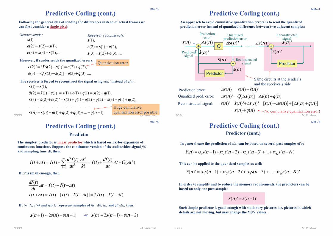
MM-73
Following the general idea of sending the differences instead of actual frames we
can first consider a single pixel:
Sender sends:
(1),
(2) (2) (1),
(3) (3) (2),....
se s se s s
= −
= −
Receiver reconstructs:
(1),
(2) (1) (2),
(3) (2) (3),....
ss s es s e
= +
= +
However, if sender sends the quantized errors:
(2) ' [ (2) (1)] (2) (2),
(3) ' [ (3) (2)] (3) (3),....
e Q s s e qe Q s s e q
= − = +
= − = +
The receiver is forced to reconstruct the signal using e(n)’ instead of e(n):
(1) (1),
(2) (1) (1) ' (1) (1) (1) (2) (1),
(3) (2) (2) ' (2) (1) (2) (2) (3) (1) (2),
. . . . . . . . . . . . . . .
( ) ( ) (1) (2) (3) ... ( 1)
s ss s e s e q s qs s e s q e q s q q
s n s n q q q q n
=
= + = + + = +
= + = + + + = + +
= + + + + + −
!
! !
! !
!
Quantization error
Huge cumulative
quantization error possible"
Predictive Coding (cont.)
SDSU M. Vuskovic
MM-74
Predictive Coding (cont.)
An approach to avoid cumulative quantization errors is to send the quantized
prediction error instead of quantized difference between two adjacent samples:
+ +
Predictor
+
+
-
( )s n ( )s n" ( ) 's n"
�( ) 's n�( ) 's n
( ) 's n
( ) 's n"
Predictor
( ) 's n�( ) 's n
Same circuits at the sender�s
and the receiver�s side
Predictedsignal
Predictionerror
Quantizedprediction error
Q
Reconstructedsignal
Reconstructedsignal
�( ) ( ) ( ) '
( ) ' [ ( )] ( ) ( )
�( ) ' ( ) ' ( ) ' [ ( ) ( )] [ ( ) ( )]
( ) ( )
s n s n s ns n Q s n s n q n
s n s n s n s n s n s n q ns n q n
= −
= ∆ = +
= + = − + +
= +
"
" "
" " "
Prediction error:
Quantized pred. error:
Reconstructed signal:
No cumulative quantization error"
SDSU M. Vuskovic
MM-75
Predictor
2
1
( ) ( )( ) ( ) ( ) ( )
"
k kk
k
d f t t df tf t t f t f t t O tdt k dt∞
=
+ = + = + +/"
" " "
The simplest predictor is linear predictor which is based on Taylor expansion of
continuous functions. Suppose the continuous version of the audio/video signal f(t)
and sampling time ∆t, then:
If ∆t is small enough, then
( )( ) ( )
( ) ( ) [ ( ) ( )] 2 ( ) ( )
df t t f t f t tdtf t t f t f t f t t f t f t t
≈ − −
+ ≈ + − − = − −
" "
" " "
If s(n+1), s(n) and s(n-1) represent samples of f(t+∆t), f(t) and f(t-∆t), then:
( 1) 2 ( ) ( 1)s n s n s n+ ≈ − − ( ) 2 ( 1) ( 2)s n s n s n≈ − − −or
Predictive Coding (cont.)
SDSU M. Vuskovic
MM-76
Predictor (cont.)
In general case the prediction of s(n) can be based on several past samples of s:
1 2 3�( ) ( 1) ( 2) ( 3) ... ( )Ks n s n s n s n s n K= α − + α − + α − + + α −
This can be applied to the quantized samples as well:
1 2 3�( ) ' ( 1) ' ( 2) ' ( 3) ' ... ( ) 'Ks n s n s n s n s n K= α − + α − + α − + + α −
In order to simplify and to reduce the memory requirements, the predictors can be
based on only one past sample:
�( ) ' ( 1) 's n s n= −
Such simple predictor is good enough with stationary pictures, i.e. pictures in which
details are not moving, but may change the YUV values.
Predictive Coding (cont.)
SDSU M. Vuskovic
MM-77
+
Predictor
+
+-
( )s n ( )s n" ( ) 's n"
�( ) 's n�( ) 's n
( ) 's n
Q
DPCM( )s n ( ) 's n"
DPCM
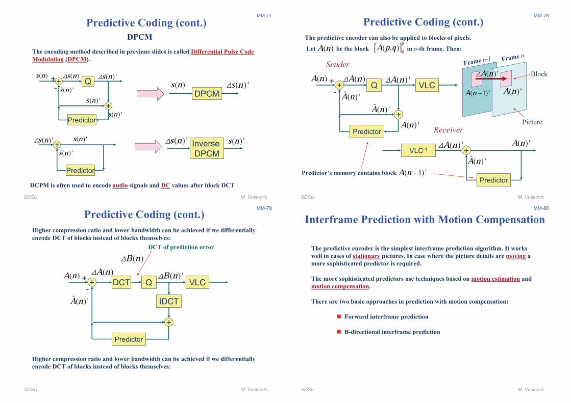
The encoding method described in previous slides is called Differential Pulse Code
Modulation (DPCM).
DCPM is often used to encode audio signals and DC values after block DCT
+( ) 's n"
Predictor
( ) 's n�( ) 's n
Inverse
DPCM
( ) 's n" ( ) 's n
Predictive Coding (cont.)
SDSU M. Vuskovic
MM-78
+( ) 'A n"
Predictor
( ) 'A n�( ) 'A n
+
Predictor
+
+
-
( )A n ( )A n" ( ) 'A n"
�( ) 'A n�( ) 'A n
( ) 'A n
Q VLC
The predictive encoder can also be applied to blocks of pixels.
Let be the block in n-th frame. Then:[ ]8
8( , )A p q( )A n
VLC-1
Sender
Receiver
Predictor’s memory contains block ( 1) 'A n −
( ) 'A n( 1) 'A n −
Frame n-1 Frame n
( ) 'A n" Block
Picture
Predictive Coding (cont.)
SDSU M. Vuskovic
MM-79
Higher compression ratio and lower bandwidth can be achieved if we differentially
encode DCT of blocks instead of blocks themselves:
+
+
+
-
( )A n ( )A n" ( ) 'B n"
�( ) 'A nVLCQ
IDCT
DCT
Predictor
( )B n"
DCT of prediction error
Higher compression ratio and lower bandwidth can be achieved if we differentially
encode DCT of blocks instead of blocks themselves:
Predictive Coding (cont.)
SDSU M. Vuskovic
MM-80
Interframe Prediction with Motion Compensation
The predictive encoder is the simplest interframe prediction algorithm. It works
well in cases of stationary pictures. In case where the picture details are moving a
more sophisticated predictor is required.
The more sophisticated predictors use techniques based on motion estimation and
motion compensation.
There are two basic approaches in prediction with motion compensation:
" Forward interframe prediction
" B-directional interframe prediction
SDSU M. Vuskovic
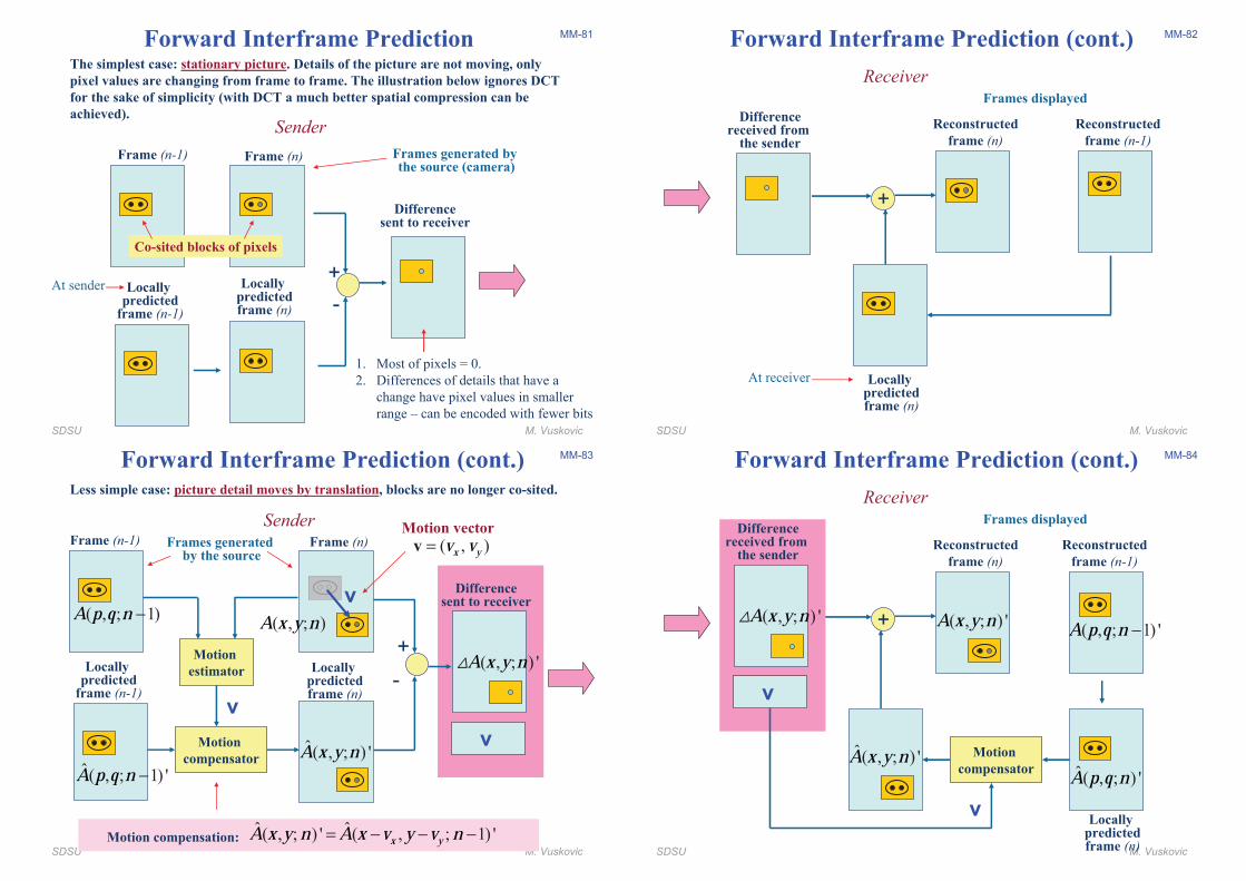
MM-81Forward Interframe PredictionThe simplest case: stationary picture. Details of the picture are not moving, only
pixel values are changing from frame to frame. The illustration below ignores DCT
for the sake of simplicity (with DCT a much better spatial compression can be
achieved).
Frame (n-1)
Differencesent to receiver
Frame (n)
Sender
Co-sited blocks of pixels
1. Most of pixels = 0.
2. Differences of details that have a
change have pixel values in smaller
range � can be encoded with fewer bits
Locallypredicted
frame (n-1)
+
-Locally
predictedframe (n)
Frames generated by the source (camera)
At sender
SDSU M. Vuskovic
MM-82Forward Interframe Prediction (cont.)
Differencereceived from
the sender
Reconstructed
frame (n)
Receiver
+
Frames displayed
At receiver Locallypredictedframe (n)
Reconstructed
frame (n-1)
SDSU M. Vuskovic
MM-83Forward Interframe Prediction (cont.)Less simple case: picture detail moves by translation, blocks are no longer co-sited.
Frame (n-1)
Differencesent to receiver
Frame (n)
Sender
Locallypredicted
frame (n-1)
+
-Locally
predictedframe (n)
Motion
estimator
Motion
compensator
v
Motion vector
( , )x yv v=v
v
Frames generated by the source
( , ; 1)A p q n −( , ; )A x y n
�( , ; 1) 'A p q n −
�( , ; ) 'A x y n
( , ; ) 'A x y n"
� �( , ; ) ' ( , ; 1) 'x yA x y n A x v y v n= − − −Motion compensation:
v
SDSU M. Vuskovic
MM-84Forward Interframe Prediction (cont.)
Reconstructed
frame (n)
Receiver
+
Frames displayed
Locallypredictedframe (n)
Reconstructed
frame (n-1)
Differencereceived from
the sender
( , ; ) 'A x y n"
v
Motion
compensator
v
( , ; ) 'A x y n( , ; 1) 'A p q n −
�( , ; ) 'A p q n�( , ; ) 'A x y n
SDSU M. Vuskovic
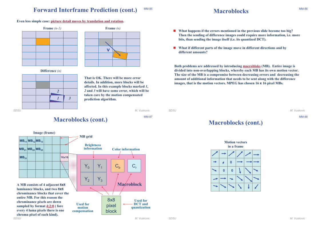
MM-85Forward Interframe Prediction (cont.)
v
Even less simple case: picture detail moves by translation and rotation.
Frame (n-1) Frame (n)
1
2
3
Difference (n)
That is OK. There will be more error
details. In addition, more blocks will be
affected. In this example blocks marked 1,
2 and 3 will have some error, which will be
taken care by the motion compensated
prediction algorithm.
SDSU M. Vuskovic
MM-86
Macroblocks
" What happens if the errors mentioned in the previous slide become too big?
Then the sending of difference images could require more information, i.e. more
bits, than sending the image itself (i.e. its quantized DCT).
" What if different parts of the image move in different directions and by
different amounts?
Both problems are addressed by introducing macrobloks (MB). Entire image is
divided into non-overlapping blocks, whereby each MB has its own motion vector.
The size of the MB is a compromise between decreasing errors and decreasing the
amount of additional information that needs to be sent along with the difference
images, that is the motion vectors. MPEG has chosen 16 x 16 pixel MBs.
SDSU M. Vuskovic
MM-87
A MB consists of 4 adjacent 8x8
luminance blocks, and two 8x8
chrominance blocks that cover the
entire MB. For this reason the
chrominance pixels are down
sampled by format 4:2:0 ( fore
every 4 luma pixels there is one
chroma pixel of each kind).
Image (frame)
16x16
Y0 Cb CrY1
Y2 Y3
8x8
pixel
block
Macroblock
Brightness information
MB grid
Color information
Used for DCT and
quantizationUsed for motion
compensation
MB11 MB12 MB13
MB21 MB22 MB23
MB31
Macroblocks (cont.)
SDSU M. Vuskovic
MM-88
Motion vectors
in a frame
Macroblocks (cont.)
0
0 0
SDSU M. Vuskovic
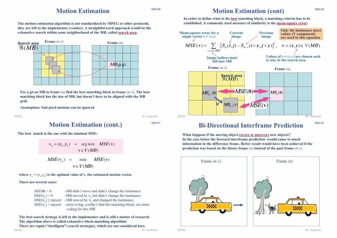
MM-89Motion Estimation
The motion estimation algorithm is not standardized by MPEG or other protocols,
they are left to the implementer (vendor). A straightforward approach would be the
exhaustive search within some neighborhood of the MB, called search area.
For a given MB in frame (n) find the best matching block in frame (n-1). The best
matching block has the size of MB, but doesn’t have to be aligned with the MB
grid.
Assumption: Sub pixel motions can be ignored
Frame (n)Frame (n-1)
( , )MB p q
Search area
( )MBℜ
SDSU M. Vuskovic
MM-90Motion Estimation (cont)In order to define what is the best matching block, a matching criteria has to be
established. A commonly used measure of similarity is the mean-square error:
Frame (n)Frame (n-1)
( )nMB 01( )nMB − 0
1( )nMB − vv
Search area ( )MBℜ
( )MSE 0
( )MSE v
[ ]2
1
( , )
( ) ( , ) ( , ) , ( , ) V( )n ni j MB
MSE S i j S i x j y x y MB−
∈
= − + + = ∈/v v
Currentimage
Previousimage
Mean-square error for a single vector v = (x,y)
Image indices must fall into MB
Values of v = (x,y) are chosen such to stay in the search area
Only the luminance pixel values (Y component) are used in this equation.
SDSU M. Vuskovic
MM-91Motion Estimation (cont.)
The best match is the one with the minimal MSE:
( , ) arg min ( )
( )
o o ox y MSEV MB
= =
∈
v v
v
There are several cases:
MSE(0) = 0 - MB didn�t move and didn�t change the luminance
MSE(vo) = 0 - MB moved by vo but didn�t change the luminance
MSE(vo) ! maxerr - MB moved by vo and changed the luminance
MSE(vo) > maxerr - error to big, couldn�t find the matching block, use intra-
coding for this MB
( ) min ( )
( )
oMSE MSEV MB
=
∈
v v
v
where vo = (xo,yo) is the optimal value of v, the estimated motion vector.
The best search strategy is left to the implementer and is still a matter of research.
The algorithm above is called exhaustive block-matching algorithm.
There are rapid (“intelligent”) search strategies, which are not considered here.SDSU M. Vuskovic
MM-92
Bi-Directional Interframe Prediction
Frame (n-1) Frame (n)
What happens if the moving object covers or uncovers new objects?
In the case below the forward interframe prediction would cause to much
information in the difference frame. Better result would have been achieved if the
prediction was based on the future frame (n) instead of the past frame (n-1).
SDSU M. Vuskovic
MM-93
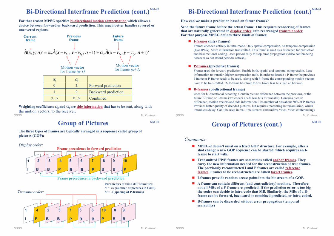
Bi-Directional Interframe Prediction (cont.)
For that reason MPEG specifies bi-directional motion compensation which allows a
choice between forward or backward prediction. This much better handles covered or
uncovered regions.
� � �( , ; ) ' ( , ; 1) ' ( , ; 1) 'b bx by f fx fyA x y n A x v y v n A x v y v n= α − − − + α − − +
Motion vectorfor frame (n-1)
Current frame
Previousframe
Future frame
Motion vectorfor frame (n+1)
0.5
1
0
αb
Combined0.5
Backward prediction0
Forward prediction1
αf
Weighting coefficients αb and αf are side information that has to be sent, along with
the motion vectors, to the receiver.SDSU M. Vuskovic
MM-94
Bi-Directional Interframe Prediction (cont.)
How can we make a prediction based on future frames?
Send the future frame before the actual frame. This requires reordering of frames that are naturally generated in display order, into rearranged transmit order.For that purpose MPEG defines three kinds of frames:
" I-frames (intra frames)
Frames encoded entirely in intra-mode. Only spatial compression, no temporal compression
(like JPEG). More information transmitted. This frame is used as a reference for predictive
and bi-directional coding. Used periodically to stop error propagation (video conferencing
however ca not afford periodic refresh).
" P-frames (predictive frames)
Frames used for forward prediction. Enable both, spatial and temporal compression. Less
information to transfer, higher compression ratio. In order to decode a P-frame the previous
I-frame or P-frame needs to be used. Along with P-frame the corresponding motion vectors
have to be transmitted. A P-frame has three to five times less bits than an I-frame.
" B-frames (bi-directional frames)
Used for bi-directional decoding. Contain picture difference between the previous, or the
future P-frame or I-frame (whichever needs less bits for transfer). Contains picture
difference, motion vectors and side information. Has number of bits about 50% of P-frames.
Provides better quality of decoded pictures, but requires reordering in transmission, which
introduces delay. Can�t be used in real-time streams (interactive video, video conferencing)
SDSU M. Vuskovic
MM-95Group of PicturesThe three types of frames are typically arranged in a sequence called group of
pictures (GOP):
I
1
B
2
B
3
P
4
B
5
B
6
P
7
B
8
B
9
P
10
I
1
P
4
B
2
B
3
P
7
B
5
B
6
P
10
B
8
B
9
Display order:
Transmit order:
Frame precedence in forward prediction
Frame precedence in backward prediction
Parameters of this GOP structure:
N = 10 (number of pictures in GOP)
M = 3 (spacing of P-frames)
SDSU M. Vuskovic
MM-96
Comments:
" MPEG-2 doesn’t insist on a fixed GOP structure. For example, after a shot change a new GOP sequence can be started, which requires an I-frame to start with.
" Transmitted I/P/B frames are sometimes called anchor frames. They carry the new information needed for the reconstruction of true frames. The previously reconstructed I and P frames are called reference frames. Frames to be reconstructed are called target frames.
" I-frames provide random access point into the bit stream of a GOP.
" A frame can contain different (and contradictory) motions. Therefore not all MBs of a P-frame are predicted. If the prediction error is too big the coder can decide to intra-code that MB. Similarly, the MBs of a B-frame can be forward, backward or combined predicted, or intra-coded.
" B-frames can be discarded without error propagation (temporal scalability)
Group of Pictures (cont.)
SDSU M. Vuskovic
MM-97Group of Pictures (cont.)
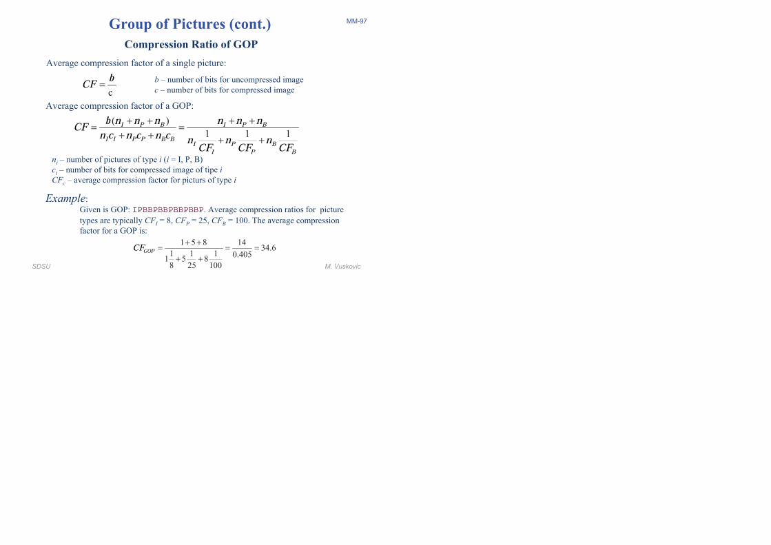
Compression Ratio of GOP
Average compression factor of a single picture:
c
bCF =b � number of bits for uncompressed image
c � number of bits for compressed image
Average compression factor of a GOP:
( )
1 1 1I P B I P B
I I P P B B I P BI P B
b n n n n n nCF n c n c n c n n nCF CF CF
+ + + += =
+ ++ +
ni � number of pictures of type i (i = I, P, B)
ci � number of bits for compressed image of tipe i
CFc � average compression factor for picturs of type i
Example: Given is GOP: IPBBPBBPBBPBBP. Average compression ratios for picture
types are typically CFI = 8, CFP = 25, CFB = 100. The average compression
factor for a GOP is:
1 5 8 1434.6
1 1 1 0.4051 5 8
8 25 100
GOPCF + += = =
+ +
Recommended