RANDOM DOT PRODUCT GRAPHS
A MODEL FOR SOCIAL NETWORKS
by
Christine Leigh Myers Nickel
A dissertation submitted to The Johns Hopkins University in conformity with the
requirements for the degree of Doctor of Philosophy.
Baltimore, Maryland
December, 2006
c© Christine Leigh Myers Nickel 2006
All rights reserved

Abstract
We develop a new set of random graph models. The motivation for these mod-
els comes from social networks and is based on the idea of common interest. We
represent a social network as a graph, in which vertices correspond to individu-
als. In the general model, an interest vector xv, drawn from a specific distribu-
tion, is associated with corresponding vertex v. The edge between vertices u and
v exists with some probability P (xi, xj) = f(xu · xv); that is, it is equal to a func-
tion of the dot product of the vectors. The probability of a graph H is given by
PX[H] =
[∏uv∈E(H)
u<vf(xu · xv)
] [∏uv/∈E(H)
u<v(1− f(xu · xv))
]and is dependent upon
the distribution from which the vectors are drawn.
We examine three versions of the Random Dot Product Graph on n vertices. In the
dense model, the vectors are drawn from Ua[0, 1], the ath power (a > 1) of the uniform
distribution on [0, 1], and f is the identity function. In this case, with probability
approaching one as n approaches infinity, all fixed graphs appear as subgraphs. In
the sparse model, the vectors are again drawn from Ua[0, 1], however the probability
function is f(s) = snb (b ∈ (0,∞)). With this change, subgraphs appear at certain
ii

thresholds and we examine the sequence of their appearance. In both cases, we show
that the models obey a power law degree distribution, exhibit clustering, and have a
low diameter; these are all characteristics found in social networks.
The third version is a discrete model. Here the vectors are drawn from {0, 1}t
(t ∈ Z+)) and f(s) = st. Each coordinate of xv is independently assigned the value 1
with probability p and 0 otherwise (p ∈ [0, 1]). We define the probability order polyno-
mial, or POP, of a graph H as a function that is asymptotic to P≥[H], the probability
of H appearing as a (not necessarily induced) subgraph, and present geometric tech-
niques for studying POP asymptotics. We give a general method for calculating the
POP of H. We present formuals for the POPs and first moment results for trees,
cycles, and complete graphs. We also prove a threshold result for K3 and describe
a general method for proving threshold results when all the required POPs are known.
Advisor: Edward R. Scheinerman
Second Reader: Carey E. Priebe
iii

Acknowledgements
This research was supported in part by the Australian Defence Science Technology
Organisation; Miro Kraetzel, project officer.
I cannot possibly express in words the gratitude that I owe my advisor, Edward
Scheinerman. He is a brilliant mathematician and most excellent mentor. In addition
to his insights and guidance, I greatly appreciate his understanding and patience. I
am most thankful that he never gave up on me.
I would like to thank Professors Priebe, Wierman, and Fishkind for serving on my
dissertation committee. Not only did they offer suggestions on improving this thesis,
but they asked insightful questions and showed a true interest in this work.
In addition to my committee, Miro Kraetzel and Professor James Fill helped to
improve this work with their ideas and suggestions.
I am thankful to all of the faculty who taught or otherwise supported me during
my graduate schooling, both here at Johns Hopkins and also at the University of
Alabama in Huntsville. I would like to specifically thank Peter Slater for being my
earliest advisor and Grant Zhang for introducing me to Graph Theory.
iv

I would like to thank the current and former staff of our department, Amy
Berdann, Kristin Bechtel, Sandy Kirt, and Kay Lutz, for all their support.
I found many friends amongst my fellow graduate students and I am grateful for
them all. I would like to thank Leslie Cope for that very fist sentence. I am especially
thankful for Beryl Castello. She has been the best baby sitter, cheerleader, and friend.
I owe a deep gratitude to my family. My parents, Norm and Maryellen, and
siblings, Jay and Jenny, have always believed in and supported me; not just in this
endeavor, but in all that I do.
Finally, I am eternally thankful for my husband Lee and daughter Alexandra.
They have made many sacrifices so that I could pursue my dream, always doing
so without complaint. Lee has been the best husband possible. He has loved and
supported me in every way. He has always believed in me and I am so thankful that
he never let me quit. Lee’s love and confidence in me and Alexandra’s smile made
this dissertation a reality.
v

This dissertation is dedicated to all of my children: those who have gone before me,
those who are with me now, and those who I have yet to meet.
vi

Contents
Abstract ii
Acknowledgements iv
List of Figures ix
1 Introduction 11.1 The Motivating Problem . . . . . . . . . . . . . . . . . . . . . . . . . 11.2 A Brief History of Modeling the Internet . . . . . . . . . . . . . . . . 2
1.2.1 Early Random Graph Models . . . . . . . . . . . . . . . . . . 21.2.2 The Internet and Power Laws . . . . . . . . . . . . . . . . . . 51.2.3 Power Law Generators . . . . . . . . . . . . . . . . . . . . . . 71.2.4 The Internet as a Small World . . . . . . . . . . . . . . . . . . 10
1.3 An Overview of Things to Come . . . . . . . . . . . . . . . . . . . . . 11
2 The Dense Model 152.1 The Random Dot Product Graph – A New Model . . . . . . . . . . . 15
2.1.1 The General Model . . . . . . . . . . . . . . . . . . . . . . . . 152.2 The Dense Random Dot Product Graph . . . . . . . . . . . . . . . . 17
2.2.1 Some Results in the Simplest Case . . . . . . . . . . . . . . . 172.3 Main Results . . . . . . . . . . . . . . . . . . . . . . . . . . . . . . . 21
2.3.1 Degree Power Law . . . . . . . . . . . . . . . . . . . . . . . . 212.3.2 Clustering . . . . . . . . . . . . . . . . . . . . . . . . . . . . . 382.3.3 Diameter . . . . . . . . . . . . . . . . . . . . . . . . . . . . . 39
2.4 Higher Dimensions . . . . . . . . . . . . . . . . . . . . . . . . . . . . 472.4.1 Basic Results in Higher Dimensions . . . . . . . . . . . . . . . 472.4.2 A Bend in the Power Law . . . . . . . . . . . . . . . . . . . . 51
3 The Sparse Model 563.1 The Sparse Random Dot Product Graph . . . . . . . . . . . . . . . . 57
vii

3.1.1 Results in the General Case: b ∈ (0,∞) . . . . . . . . . . . . . 573.1.2 Results when b ∈ (0, 1) . . . . . . . . . . . . . . . . . . . . . . 693.1.3 The Land of Trees: b ∈ (1, 2) . . . . . . . . . . . . . . . . . . . 78
3.2 Main Results . . . . . . . . . . . . . . . . . . . . . . . . . . . . . . . 873.2.1 The Threshold Result . . . . . . . . . . . . . . . . . . . . . . 873.2.2 Degree Distribution . . . . . . . . . . . . . . . . . . . . . . . . 923.2.3 Diameter . . . . . . . . . . . . . . . . . . . . . . . . . . . . . 110
3.3 The Complete Picture . . . . . . . . . . . . . . . . . . . . . . . . . . 119
4 Posynomial Asymptotics: A Prelude to the The Discrete Model 1224.1 The β, α Parameter Space . . . . . . . . . . . . . . . . . . . . . . . . 1224.2 The Equivalence Classes . . . . . . . . . . . . . . . . . . . . . . . . . 1274.3 Dividing Lines . . . . . . . . . . . . . . . . . . . . . . . . . . . . . . . 138
5 The Discrete Model 1535.1 The 0, 1 Discrete Random Dot Product Graph . . . . . . . . . . . . . 154
5.1.1 Basic Results . . . . . . . . . . . . . . . . . . . . . . . . . . . 1555.1.2 K3 : A Detailed Example . . . . . . . . . . . . . . . . . . . . 163
5.2 The Probability Order Polynomial . . . . . . . . . . . . . . . . . . . . 1685.2.1 Defining the POP . . . . . . . . . . . . . . . . . . . . . . . . . 1685.2.2 POPs of Trees, Cycles, and Complete Graphs . . . . . . . . . 177
5.3 Towards a Threshold Result . . . . . . . . . . . . . . . . . . . . . . . 1965.3.1 The First Moment . . . . . . . . . . . . . . . . . . . . . . . . 1965.3.2 Threshold Theory . . . . . . . . . . . . . . . . . . . . . . . . . 214
6 Overview and Directions for Future Work 2316.1 Observations and New Directions . . . . . . . . . . . . . . . . . . . . 232
6.1.1 The Dense Random Dot Product Graph . . . . . . . . . . . . 2326.1.2 The Sparse Random Dot Product Graph . . . . . . . . . . . . 2346.1.3 The Discrete Random Dot Product Graph . . . . . . . . . . . 237
6.2 Other Open Problems and Thoughts for Future Work . . . . . . . . . 2406.2.1 General Graph Theory Questions . . . . . . . . . . . . . . . . 2406.2.2 Variations on the Model . . . . . . . . . . . . . . . . . . . . . 2416.2.3 In Conclusion . . . . . . . . . . . . . . . . . . . . . . . . . . . 242
Bibliography 244
Vita 248
viii

List of Figures
2.1 The domain U(b) . . . . . . . . . . . . . . . . . . . . . . . . . . . . . 53
4.1 The line li : h− xiα− β i = 0. . . . . . . . . . . . . . . . . . . . . . . 1244.2 (a) The lines associated with fα,β,h(n). (b) C(f) and ζ(f). . . . . . . 1264.3 If (β0, α0) ∈ C(f) then all points (β, α) ≥ (β0, α0) are in C(f). . . . . 1284.4 The lines li, li,j and lj. . . . . . . . . . . . . . . . . . . . . . . . . . . 1374.5 Case 1: The region A. . . . . . . . . . . . . . . . . . . . . . . . . . . 1424.6 Case 1 with (a) xi > yj and the slope of l3 positive. (b) xi < yj and
the slope of l3 negative. . . . . . . . . . . . . . . . . . . . . . . . . . . 1444.7 Case 2: The region A′. . . . . . . . . . . . . . . . . . . . . . . . . . . 1454.8 Case 3: The region A′′. . . . . . . . . . . . . . . . . . . . . . . . . . . 1464.9 Case 3 with βint < 0 and (a) xi > yj. (b) xi = yj. (c) xi < yj and
i < j. (d) xi < yj and i = j. (e) xi < yj and i > j. . . . . . . . . . . 1474.10 Case 4: The region A′′. . . . . . . . . . . . . . . . . . . . . . . . . . . 149
5.1 (a) The lines that define C(f′T ). (b) li intersects C(fT ) at exactly one
point. . . . . . . . . . . . . . . . . . . . . . . . . . . . . . . . . . . . 1995.2 (a) The lines that define C(f
′Ch). (b) li is ‘below’ C(fCh). . . . . . . 2035.3 The lines that define C(f
′Kh). . . . . . . . . . . . . . . . . . . . . . . 2075.4 The line lk is ‘below’ C(fCh). . . . . . . . . . . . . . . . . . . . . . . . 2105.5 The graph Hkite. . . . . . . . . . . . . . . . . . . . . . . . . . . . . . 2115.6 (a) All of the lines associated with terms of fHkite . (b) C(fHkite) and
ζ(fHkite). . . . . . . . . . . . . . . . . . . . . . . . . . . . . . . . . . . 2135.7 The dotted lines are those associated with terms of g∗α,β,4(n) and are
all ‘below’ C(f′K3). . . . . . . . . . . . . . . . . . . . . . . . . . . . 219
5.8 The dotted lines are those associated with terms of g∗∗α,β,5(n) and areall ‘below’ C(fK3). . . . . . . . . . . . . . . . . . . . . . . . . . . . . 220
5.9 The graph H2−kite. . . . . . . . . . . . . . . . . . . . . . . . . . . . . 2275.10 The line l(H2−kite)0 is not always ‘below’ C(fHkite). . . . . . . . . . . 228
ix

5.11 (a) The point (7/10, 10/29) ∈ C(fHkite). (b) The point (7/10, 10/29) ∈ζ(fK4). . . . . . . . . . . . . . . . . . . . . . . . . . . . . . . . . . . 229
x

Chapter 1
Introduction
In this thesis we develop a new set of random graph models. The motivation for
these models comes from social networks and is based on the idea of common interest.
1.1 The Motivating Problem
People with shared interest are more likely to communicate than those without
shared interests. Perhaps an active graph theorist is more likely to interact with an-
other discrete mathematician than with a statistician. Likewise, a drastic change in
an individual’s social relationships may reflect a corresponding change in that indi-
vidual’s lifestyle or activities. If our graph theorist suddenly begins to socialize with
literary critics, we might expect that this was due to a change in the mathematician’s
interests.
We represent a social network as a graph, in which vertices correspond to indi-
1

viduals. An interest vector xi is associated with each individual and corresponding
vertex i. The edge between vertices i and j (indicating acquaintance between the
corresponding individuals) exists with some probability P (xi, xj). The internet may
be modeled in the same way: Individual web spages are represented by vertices with
(directed) edges corresponding to hyperlinks.
We seek to develop tractable and realistic models for such graphs. A good proba-
bilistic model would lead to simulated networks whose graph theoretic characteristics
match those of naturally occurring networks. Several distinct graph theoretic fea-
tures are repeatedly observed in social networks; for example the degree distribution
typically follows a power law and the network appears to be highly clustered.
1.2 A Brief History of Modeling the Internet
The world wide web is a particularly attractive subject for network research.
Although it is a large network, techniques have been developed to collect information
about its structure. Additionally, the web is dynamic, changing continuously. Finally,
unlike other social networks, data collection may be done anonymously.
1.2.1 Early Random Graph Models
Originally attempts were made to model the physical structure of the internet.
The internet was viewed as an undirected graph in which nodes represented routers (or
2

domains) and edges represented the physical links connecting the routers (domains).
An early random graph model for the internet was proposed by Waxman in 1988
[24]. We distribute N vertices uniformly at random in the x-y coordinate plane. For
each pair of vertices, u and v, the Euclidean distance, d(u, v), is calculated and a
parameter L is defined to be the maximum value of these distances. Two additional
parameters, α, β ∈ [0, 1], are chosen by the user. The probability that the edge
between u and v is in the graph is P [u ∼ v] = β e−d(u,v)
Lα . Once all possible vertex
pairs have been considered the graph is checked for connectedness. If the graph is
found to be disconnected, then process restarts and repeats itself until a connected
graph is generated.
In 1993, Doar and Leslie [9] proposed a modification to the Waxman graph that
would allow the average degree of a vertex to remain fixed as the number nodes
increased. Again, N nodes are distributed uniformly at random in the x-y plane
and the Euclidean distances d(u, v) for each pair of vertices u and v are calculated.
However, in addition to the parameters L, α, and β of the Waxman graphs, the desired
average degree ξ, and a constant k are introduced. The constant k varies with α, β,
and ξ and is determined numerically. The probability that an edge exists between
vertices u and v is given by P [u ∼ v] = β kξN
e−d(u,v)
Lα .
Calvert et al. [8] sought a model that more closely reflects the hierarchical struc-
ture of the internet. Their model consists of a two phase process. First, N vertices
are uniformly distributed in the unit square and the Euclidean distances between
3

each pair of vertices u and v, d(u, v) is calculated. A radius R and probability α are
chosen by the user so that whenever d(u, v) ≤ R, the vertices u and v are adjacent
with constant probability α. If the distance d(u, v) is above the threshold R, the
probability of the edge between u and v decreases linearly as d(u, v) increases. The
probability that an edge exists between u and v is given by
P [u ∼ v] =
α if d(u, v) ≤ R,
α√
2−d(u,v)√2−R
if d(u, v) > R.
If the resulting graph is not connected, the process starts over. Once a connected
graph G has been generated the second phase begins.
In the second phase, the graph G determines the upper-level structure for the
final graph. Each of the N nodes in the graph G is replaced by another graph on
N vertices that is generated in the same manner as G. Edges incident to a node u
in G are connected to vertices in the new graph Gu that replaced u in G as follows:
order the vertices of Gu in increasing order of degree ignoring all vertices of degree 1;
connect the edges in the upper-level graph that are adjacent to u in G to the vertices
in Gu, one edge per vertex, sequentially with respect to the above ordering. The
resulting graph will have N2 vertices. The process can be easily generalized to create
a graph with multiple levels.
Another hierarchical generation method is the Transit-Stub method introduced
by Calvert, Doar and Zegura [7]. The basic idea is that a connected random graph is
4

generated using any of the above methods. Then each vertex in the graph represents a
transit domain and is replaced by another randomly generated, connected graph Gtd.
Then, for each vertex in a transit domain graph Gtd, a collection of random graphs
is generated and attached to its transit domain vertex. These graphs represent the
stub domains. Finally, extra edges are added between stub domains or stub domains
and transit domains. This generates a random graph with the desired hierarchy.
Other models have been proposed [25], however they mainly consist of adaptations
to these basic ideas. Additionally, canonical networks such as the rings, paths, the
rectangular grid and the Erdos-Renyi random graphs have been studied, but deemed
unrealistic for this application [21, 25].
1.2.2 The Internet and Power Laws
In August of 1999, Faloutsos et al. released a technical report that changed
the way in which modelers viewed the internet [10]. They looked at three domain
level “snapshots” of the physical (interdomain) topology of the internet taken during
the period from November 1997 to December 1998. During this time the internet
experienced 45% growth. They concluded that internet exhibited at least 3 different
power law relationships.
The first of these power laws relates the out-degree dv of a vertex v to the rank
rv of the vertex, where a vertex corresponds to an internet domain. The rank of a
vertex v is the index of v when the vertices are listed in decreasing order of out-degree.
5
They showed that when all vertices of out-degree zero are ignored, dv ∝ rRv where R,
the rank exponent, is the slope of the log-log plot of (rv, dv). The next power law is
the degree distribution power law. This law illustrates the relationship between the
frequency fd of the out degree d to d. Again, ignoring vertices of out-degree zero,
it was found that fd ∝ dφ where the out-degree exponent φ is the slope of the log-
log plot of (fd, d) and is negative. Faloutsos et al. felt that this power law was the
most important since the data supported it most closely. A third power law relates
the positive eigenvalues of the adjacency matrix of the internet graphs to their index
when listed in decreasing order, i.e., λi ∝ iε.
Power laws are also exhibited elsewhere in the World Wide Web structure. If the
web is modelled as a directed graph in which vertices represent documents and edges
represent hyperlinks from one document to another, then Albert et al. [3] found that
the frequency fd of an out-degree d was again inversely proportional to a power of the
degree d and that this relationship is a power law. Independently, Kleinberg et al.
obtained the same results [15]. Huberman and Adamic also found that the number
of web pages at each of the web sites exhibits a power law behavior similar to the
Faloutsos rank versus out-degree relationship [12]. These results shifted interest in
the modeling community away from hierarchy and towards degree distribution.
6

1.2.3 Power Law Generators
Although Faloutsos et al. [10] discovered power laws inherent in the internet,
they did not attempt to explain why the behavior occurred. Two basic causes for
the degree distribution power law were suggested by Barabasi and Albert [4]. The
first is that the web exhibits incremental growth, that is the size of the network is
gradually increased over time by the continual addition of new vertices. The second
idea is that of preferential connectivity, or the increased likelihood that a new vertex
will be adjacent to an existing vertex of higher degree.
Medina, Matta, and Byers [16] proposed a parameterized topology generator that
allows the user to study the causes suggested by Barabasi and Albert. Their model
BRITE (for Boston University Representative Internet Topology Generator) divides
the x-y plane into equally sized “high-level” squares. Each high-level square is sub-
divided into equally sized “low-level” squares. The number of vertices n to be placed
in each high-level square is determined by a specific distribution. The n vertices are
then distributed uniformly in the high-level square ensuring that at most one vertex
is placed in each low-level square. BRITE has three parameters that control how ver-
tices are connected. The parameter m determines the number of neighbors to which
a new vertex will be connected when it first joins the graph. The incremental growth
parameter can either be INACTIVE: that is, all of the vertices will be placed in the
plane before any of the edges are added and then at each step a vertex is randomly
selected and attached to m other vertices in the plane; or ACTIVE: here a small
7

randomly connected backbone of m0 vertices is initially generated and then all other
vertices are added one at a time and connected to vertices that are already in the
graph. Finally, the preferential connectivity parameter controls the probability that
two vertices will be adjacent. If the preferential connectivity is set to NONE: then
the Waxman probability function is used; if set to ONLY: then a vertex v, when first
considered, will connect to a possible neighbor u with probability P [v ∼ u] = duPx∈C dx
where du is the degree of vertex u, and C is the collection of possible neighbors; if
set to BOTH: then the vertices are adjacent based on a combination of Waxman’s
probability wv∼u and the above preference for already highly connected nodes, so that
P [u ∼ v] = wu duPx∈C wx dx
. They found that the preferential connectivity and incremen-
tal growth were both needed to ensure that the graphs generated obey the degree
distribution power law.
Another model for producing graphs that obey the degree distribution power law
was proposed by Aiello, Chung, and Lu [2]. Their model has two parameters, α and
β, that control the size and growth rate of the graph. They generate a random graph
with a degree distribution that obeys the following: For a given degree d, the number
of vertices fd of degree d is given by fd = b eα
dβ c. They assume no isolated vertices. To
generate their graphs for each vertex v, they create a set Lv containing d(v) copies
of v. Next, they find a random matching on the vertices in L =⋃
v Lv. Finally, they
collapse each Lv into a single vertex so that for any two vertices u and v, the number
of edges between u and v is equal to the number of edges in the matching between
8
vertices in Lu and vertices in Lv.
A third generator was developed by Jin, Chen, and Jamin [13]. The generator
uses the desired number of vertices N and the percentage k of the vertices that are
of degree one to calculate the degree and rank distributions based on the Faloutsos
power laws. Next a spanning tree is generated among all the vertices of degree at least
two, by beginning with the empty graph G and uniformly at random selecting a node
not yet in G to be added. The new vertex v will be adjacent to an existing vertex
u in G, that is not already adjacent to d(u) vertices, with probability proportional
to the to the current degree of u in G. Next the nodes of degree one are added to
G in the same manner. Finally, any remaining vertices with degrees that have not
been satisfied are connected, beginning with the vertex of highest degree, with the
same proportional probabilities. A feasibility check is used to ensure that the graph
is connected.
Additionally, in a vein similar to ours, others have attempted to model social
networks such as the internet by assigning vertices to points in space and determining
their adjacency based on these positions. Hoff, Raftery, and Handcock [11] propose
such a latent position model. In their model, they allow differing levels of adjacency
between vertices and represent the social network as a matrix Y with entries yu,v
indicated the level of affinity between actors u and v. Thus, one can think of Y as the
adjacency matrix representation of a graph with weighted edges. For a fixed Y , the
probability of a realization of Y is given by P (Y |Z, X, θ) =∏
u 6=v P (yu,v|zu, zv, xu,v, θ)
9

and is dependent upon Z, the positions associated with the vertices, X, additional
covariate information, and θ, a model parameter. Hoff et al. discuss two specific
latent position models. In both models θ = [α, β]. In the first model, the probability
of the adjacency yu,v depends on the Euclidean distance between zu and zv (the
positions associated with u and v), specifically, the probability of yu,v depends on
α + β · xu,v − |zu − zv|. In their second model, the probability of the adjacency yu,v
depends upon zu ·zv/|zv|, the signed magnitude of the projection of zu in the direction
of zv, specifically, α + β · xu,v + zu·zv
|zv | .
Other models have been suggested [5, 6, 18], however they are similar to those
listed above. There has been some work done comparing the different random graph
based models for the internet [6, 21, 25]. Several metrics that have been suggested
include diameter, number of biconnected components, eccentricity distribution, k-
neighborhood size distribution, and clustering coefficients.
1.2.4 The Internet as a Small World
The notion of small world phenomenon, or the idea that any two people can be
related through a relatively short chain of acquaintances, has been present in social
theory for decades [17]. However the idea of small world graph was introduced by
Watts and Strogatz [23]. Some basic definitions are needed to describe a small world
graph [22]. Consider a graph G = (V, E). For each vertex v ∈ V let ρ(v) =P
u∈V d(u,v)
|V |−1
where d(u, v) is the number of edges in a shortest path between u and v. Then ρ(v)
10

is the average shortest path length from v to any other vertex. Let the characteristic
path length, LG be the median of the ρ(v)’s. Next we define the clustering coefficient
γ(v) for each v ∈ V as
γ(v) =|E(N(v))|
|N(v)|
2
where N(v) is the open neighborhood of v. Then the clustering coefficient γG for the
graph G is the mean of {γ(v) : |N(v)| ≥ 2}. Finally, let R(n, k) be the random graph
on n vertices with average degree k constructed by beginning with the empty graph
on n vertices and uniformly at random choosing two vertices to connect with an edge
until the graph contains n k2
edges. Then a small world graph is a graph G on n
vertices with average degree k for which LG ≈ LR(n,k) ≈ log(n)log(k)
, but γG À γR(n,k) ≈ kn,
that is a graph for which the characteristic path length is small and similar to that
of a random graph, but whose vertices are highly clustered.
It has been noted that the world wide web exhibits small word behavior [1, 6].
1.3 An Overview of Things to Come
This thesis introduces and examines the Random Dot Product Graph suite of
models. Three sets of models for social networks, all based on the idea of common or
shared interest are discussed. The first model, discussed in Chapter 2, is the Dense
Random Dot Product Graph. In this model, with probability approaching one as
11

the number of vertices approaches infinity, all small subgraphs appear. The second
model, discussed in Chapter 3, is the Sparse Random Dot Product Graph and small
subgraphs appear at certain thresholds. Finally, the third model is a discrete version
and is discussed in Chapter 5. As in the sparse model, in the Discrete Random Dot
Product Graph small subgraphs appear at various thresholds.
More specifically, Chapter 2 introduces the general Random Dot Product Graph.
We begin by defining and discussing the basic model. We then focus on the Dense
Random Dot Product Graph, starting by presenting simple results. The bulk of the
chapter is spent proving the three main results in the dense case. First in Section
2.3.1, we show that the model obeys the degree distribution power law observed in
World Wide Web [10]. Secondly in Section 2.3.2, we show that the model exhibits
clustering, i.e., two vertices are more likely to be adjacent if they have a common
neighbor. In social networks clustering translates into the idea that two people who
share a common friend are more likely to know each other than people who do not.
Thirdly in Section 2.3.3, we show that the Dense Random Dot Product Graph has
a low fixed diameter of at most six. Finally, we end the chapter by extending the
Dense Random Dot Product Graph into higher dimensions. We prove some results
similar to those in a single dimension and discuss a bend that occurs in the degree
distribution power law.
Chapter 3 discusses the Sparse Random Dot Product Graph. In Section 3.1.1, the
sparse version of the model is introduced and simple results are proved. The main
12

results parallel those in the dense case and are presented in Section 3.2. We show
that under certain restrictions, the sparse model obeys the degree power law, exhibits
clustering, and has a small diameter. Additionally, unlike in the dense model where
all small subgraphs appear with probability tending to one, in the sparse model
subgraphs appear at certain thresholds dependent upon a parameter b that is not
present in the dense version. We present specific results regarding the thresholds for
the appearance of edges, cliques, cycles, and trees and discuss the evolution of the
Sparse Random Dot Product Graph as b goes from zero to infinity. Then in Section
3.2.1, we prove a general threshold result for the appearance of any graph H.
In Chapter 4 we briefly step away from the Random Dot Product Graphs to build
a framework for the discussion of the discrete version of the model. A class of posyn-
omials is introduced and an equivalence relation developed. Geometric techniques for
studying the asymptotics of these posynomials is presented. These techniques will be
used in Chapter 5 in first and second moment calculations.
Chapter 5 discusses the Discrete Random Dot Product Graph. In Section 5.1.1,
the discrete version of the model is presented and a few basic results are proved.
Unlike in the basic dense and sparse versions, we do not only consider the dimension
one case, but instead draw the vectors from dimension t ≥ 1. In Section 5.1.2, we
illustrate the calculation for the threshold for the appearance of K3 as a subgraph.
In Section 5.2, we define the probability order polynomial, or POP, of a graph H as
a function that is asymptotic to P≥[H], the probability of H appearing as a (not
13

necessarily induced) subgraph of a Discrete Random Dot Product Graph G. We give
a general method for calculating the POP of H and present formulas for the POPs
of trees, cycles, and complete graphs. In Section 5.3, using the framework built in
Chapter 4, we present first moment results for trees, cycles, and complete graphs.
We also prove a complete threshold result for K3 and describe a general method for
proving threshold results when all the required POPs are known.
Finally, in Chapter 6 we summarize the main results of this thesis and discuss
avenues for additional research.
14

Chapter 2
The Dense Model
2.1 The Random Dot Product Graph – A New
Model
In this thesis, we develop a set of models based on the notion that common
interests affect relationships. Additionally, we reproduce some of the leading charac-
teristics of real world social networks. The basic idea is as follows: Let G be graph
on n vertices V (G). With each vertex v ∈ V (G) we associate an interest vector xv
and the probability that vertices u and v are adjacent is dependent on xu · xv.
2.1.1 The General Model
Consider a graph G on n vertices V (G). Let t be a positive integer and let
X : V (G) → Rt be a mapping that assigns to each vertex v ∈ V (G) a vector X(v) = xv.
15

Also, let f : R → [0, 1] be a function that maps the dot products of the vectors into
probabilities. We define the Random Dot Product Graph G as follows:
• G has n vertices in V (G),
• ∀u, v ∈ V (G) the edge from u to v appears in G with probability PX[u ∼ v] =
f(xu · xv).
Let Gn = {all graphs on V = {1, . . . , n}}. We define the probability space (Gn, PX)
as follows: for any H ∈ Gn
PX[H] =
∏
uv∈E(H)u<v
f(xu · xv)
∏
uv/∈E(H)u<v
(1− f(xu · xv))
.
In the above discussion, we assume that for each vertex v ∈ V (G) we are given
the vectors xv ahead of time, and based on these vectors some probability function f
is chosen. However, we wish to model the social networks discussed above for which
no such X is yet known. So, suppose that the vectors xv are drawn independently
from some random distribution and that the graph G is then generated using an
appropriate choice of f . Then for any graph H ∈ Gn
P [H] =
∫PX[H] dX.
In this thesis, we study the behavior of the random dot product graph when the
xv’s are drawn from various distributions.
16

2.2 The Dense Random Dot Product Graph
In the rest of this chapter, we present and examine the Dense Random Dot Product
Graph, the first of three versions of the Random Dot Product Graph discussed in this
thesis. We begin by defining the model and discussing basic results. In Section
2.3.1, we show that the model obeys the degree distribution power law. In Section
2.3.2, we show that the model exhibits clustering. In Section 2.3.3, we show that the
Dense Random Dot Product Graph has a low fixed diameter of at most six. Finally
in Section 2.4, we end the chapter by extending the model into higher dimensions,
proving basic results and discussing the appearance of a bend the degree distribution
power law.
2.2.1 Some Results in the Simplest Case
We begin by looking at a relatively simple case. For each v ∈ V (G) let the vector
xv be a one-dimensional vector drawn from Ua[0, 1], the ath power (a > 1) of the
uniform distribution on [0, 1]. Then, for any v,
P [xv ≤ r] = P [ua ≤ r] = P [u ≤ r1a ] = r
1a
where r ∈ [0, 1] and u ∼ U [0, 1]. Therefore ∀ [i, j] ⊆ [0, 1],
P [xv ∈ [i, j]] =
∫ j
i
1
ax
1−aa dx
17

and the density function for xv is g(x) = 1ax
1−aa .
Now, in order to study the random dot product graph G we need to select a
probability mapping f . The simplest choice of f is the identity function, f(r) = r.
Note in the current setting, with the vectors drawn from Ua[0, 1], the identity function
does indeed map the dot products to values in [0, 1] and therefore into probabilities.
Furthermore, we interpret the vectors as a level of interest in a given topic; i.e., 0
corresponds to no interest in the topic, and 1 a very high level of interest. Here we
choose f so that if xv ·xu is near 1, indicating that both u and v have a great interest
in the topic, then the probability f(xv · xu) that they know each other is also near
1. Likewise, if xv · xu is small, we would like f(xv · xu) to be small. The identity
function achieves this. So, from now on in this chapter, we assume that f is the
identity function.
We denote this sample space of dense random dot product graphs on n vertices
in which one-dimensional interest vectors are drawn from Ua[0, 1] as D[n, a, 1]. Also,
for any u, v ∈ V (G), u ∼ v is defined as u is adjacent to v. We have the following
results.
Proposition 2.2.1. Let G be drawn from D[n, a, 1]. For any u, v ∈ V (G) we have
P [u ∼ v] = 1(a+1)2
.
18

Proof:
P [u ∼ v] =
∫ 1
0
∫ 1
0
xu xv g(xu) g(xv) dxu dxv =1
a2
∫ 1
0
∫ 1
0
x1/au x1/a
v dxu dxv =1
(a + 1)2.
QED.
So, an arbitrary edge appears in the graph with probability 1(a+1)2
and the expected
number of edges is(
n2
)1
(a+1)2.
Next, assume that n is large. We wish to study the degree distribution of G.
Proposition 2.2.2. Let G be drawn from D[n, a, 1]. The expected number of vertices
of degree zero in G is
E[|{v : d(v) = 0}|] ∼(
1
a(1 + a)
1a Γ
(1
a
))n
a−1a .
Here, Γ is the classical gamma function Γ(x) =∫∞0
tx−1e−tdt.
Proof:
Choose v ∈ V (G) fixed, but arbitrary, and denote the vector of v by y. Let
x1, x2, . . . , xn−1 be the vectors of the remaining n− 1 vertices in V (G)− {v}. Then
P [d(v) = 0] =
∫ 1
0
∫ 1
0
· · ·∫ 1
0
(1− x1y) · · · (1− xn−1y)
·g(x1) · · · g(xn−1) g(y) dx1 · · · dxn−1 dy
19

which is separable. Noting that for each of the xi’s
∫ 1
0
(1− xiy)g(xi)dxi =
∫ 1
0
1
a(1− xiy)x
1−aa
i dxi = 1− y
a + 1
we have that
P [d(v) = 0] =
∫ 1
0
(1− y
a + 1
)n−11
ay
1−aa dy.
Substituting y = y1/a for y in the integral we have that
P [d(v) = 0] =
∫ 1
0
(1− ya
a + 1
)n−1
dy.
From y = tn1/a , one has dy = dt
n1/a and 0 ≤ y ≤ 1 yields 0 ≤ t ≤ n1/a. Therefore,
substituting again we have that
P [d(v) = 0] =
∫ n1/a
0
(1− ta
(a + 1)n
)n−1dt
n1/a
∼∫ ∞
0
exp
{ −ta
a + 1
}dt
n1/a=
(1
a(1 + a)
1a Γ
(1
a
))1
n1/a.
Therefore the expected number of vertices of degree zero is
E[|{v : d(v) = 0}|] = nP [d(v) = 0] ∼(
1
a(1 + a)
1a Γ
(1
a
))n
a−1a .
QED.
We see that the expected number of isolated vertices in G is a constant times
20

na−1
a . The above result can be generalized to vertices of degree k where k ¿ n as
follows:
Proposition 2.2.3. Let k be a fixed nonnegative integer. Let λ(k) be the number of
vertices of degree k in a random dot product graph drawn from D[n, a, 1]. Then
E[λ(k)] ∼(
1
k! a(1 + a)
1a Γ
(1
a+ k
))n
a−1a
as n →∞.
2.3 Main Results
2.3.1 Degree Power Law
Now, we wish to show that the Dense Random Dot Product Graph is a good
candidate for modeling social networks, including the internet. To this end, we posit
the following.
Conjecture 2.3.1. Let ε > 0 and let n, k be integers with εn < k < (1 − ε)n.
Let λ(k) be the number of vertices of degree k in a graph drawn from D[n, a, 1].
Then as n →∞, with high probability λ(k) satisfies the degree distribution power law
λ(k) ∝ kφ, with φ = 1−aa
.
We observe that a log-log histogram of the degree distribution is a straight line
over most of the degree sequence of Dense Random Dot Product Graphs. While
21

Conjecture 2.3.1 would explain this directly, a mild relaxation of this conjecture also
explains this phenomenon. For positive integers a, b with a < b, define λ[a, b] to be
the number of vertices in a graph with degrees in the interval [a, b]. We show that
λ[k(1 − δ), k(1 + δ)] is proportional to (2kδ)kφ for most values of k and for almost
all Dense Random Dot Product Graphs (i.e., with high probability as n →∞). The
basic idea of the proof is as follows.
For a given k and δ, we want to know λ[k(1 − δ), k(1 + δ)]. However, we do not
count the number of vertices whose degrees fall in [k(1−δ), k(1+δ)] directly. Instead
we select a value s ∈ [0, 1] so that if xv = s then E[d(v)|xv = s] = (n−1)xv
a+1= (n−1)s
a+1= k
(note that this establishes a direct relationship between s and k). Then we count the
number of vertices whose vectors fall in the interval S = [s(1 − δ), s(1 + δ)], since
for any vertex v with xv ∈ S the E[d(v)|xv] = (n−1)xv
a+1∈
[(n−1)s(1−δ)
a+1, (n−1)s(1+δ)
a+1
]=
[k(1− δ), k(1 + δ)]. Likewise, if xv 6∈ S then E[d(v)|xv] 6∈ [k(1− δ), k(1 + δ)]. So, the
number of vertices with xv ∈ S is expected to be the same as the number of vertices
with d(v) ∈ [k(1− δ), k(1 + δ)].
Now, to allow for the variance that occurs in our model, we look at intervals
S− and S+ that are slightly smaller and larger than S, respectively. We show that
{v : xv ∈ S−} ⊆ {v : d(v) ∈ [k(1 − δ), k(1 + δ)]} ⊆ {v : xv ∈ S+}, each containment
occurring with high probability. And therefore, the number of vertices whose degrees
fall in [k(1− δ), k(1 + δ)] must be bounded by the number of vertices whose vectors
fall in S− and S+.
22

Before we begin, we define an X-labeled Dense Random Dot Product Graph. As
with an ordinary Dense Random Dot Product Graph, for each v ∈ V (G), let the vector
xv be a one-dimensional vector drawn from Ua[0, 1] and let the probability mapping f
be the identity function. Additionally, let X be the 1×n matrix of vectors. We denote
this sample space of X-labeled Dense Random Dot Product Graphs on n vertices as
D[X]. Note that the only difference between G ∈ D[n, a, 1] and (G,X) ∈ D[X] is that
when G is a X-labeled Dense Random Dot Product Graph the vectors are retained.
Lemma 2.3.2. Let (G,X) be drawn from D[X]. Let s ∈ (n−1/24, 1), δ = n−1/12, and
ε = n−1/3. Define the interval S− = [ s(1−δ)1−ε
, s(1+δ)1+ε
]. Then
µS− = E[d(v)|xv ∈ S−] ∈[s(1− δ)(n− 1)
(1− ε)(a + 1),s(1 + δ)(n− 1)
(1 + ε)(a + 1)
].
Proof:
µS− = E[d(v)|xv ∈ S−] = E
∑
w∈V (G) : w 6=v
I {v ∼ w|xv ∈ S−}
= (n− 1)P [v ∼ w|xv ∈ S−]
= (n− 1)
∫ s(1+δ)1+ε
s(1−δ)1−ε
∫ 1
0xvxug(xv)g(xu)dxvdxu
∫ s(1+δ)1+ε
s(1−δ)1−ε
g(xv)dxv
= (n− 1)
(∫ s(1+δ)1+ε
s(1−δ)1−ε
xvg(xv)dxv
) (∫ 1
0xug(xu)dxu
)
∫ s(1+δ)1+ε
s(1−δ)1−ε
g(xv)dxv
.
23
We look at each of the integrals separately. First note that∫ 1
0xug(xu)dxu = 1
a+1.
Next we note that
∫ s(1+δ)1+ε
s(1−δ)1−ε
g(xv)dxv =
[(s(1 + δ)
1 + ε
) 1a
−(
s(1− δ)
1− ε
) 1a
]=
[δ1
as∗
1a−1
]
for δ =(
s(1+δ)1+ε
)−
(s(1−δ)1−ε
)and some s∗ ∈
[s(1−δ)1−ε
, s(1+δ)1+ε
]by the mean value theorem.
Similarly∫ s(1+δ)
1+ε
s(1−δ)1−ε
xvg(xv)dxv =1
1 + a
[δa + 1
as∗∗
1a
]
for some s∗∗ ∈[
s(1−δ)1−ε
, s(1+δ)1+ε
].
So we have
µS− =(n− 1)
(a + 1)
1a+1
[δ a+1
as∗∗
1a
][δ 1
as∗
1a−1
] =(n− 1)
(a + 1)s∗1−
1a s∗∗
1a .
Now(
s(1−δ)1−ε
)≤ s∗, s∗∗ ≤
(s(1+δ)1+ε
). Therefore
(s(1−δ)1−ε
)≤ s∗1−
1a s∗∗
1a ≤
(s(1+δ)1+ε
).
So, we have
s(1− δ)
1− ε
n− 1
a + 1≤ µS− ≤
s(1 + δ)
1 + ε
n− 1
a + 1.
QED.
We have bounded the expected degree of any vertex whose vector falls in S−.
Lemma 2.3.3. Let (G,X) be drawn from D[X]. Let s,S−, µS− , δ and ε be defined as
in Lemma 2.3.2. Let v ∈ V (G). If s(1−δ)1−ε
≤ xv ≤ s(1+δ)1+ε
, then with probability tending
24

to 1 as n →∞
d(v) ∈[s(1− δ)(n− 1)
a + 1,s(1 + δ)(n− 1)
a + 1
].
Indeed the probability d(v) 6∈[
s(1−δ)(n−1)a+1
, s(1+δ)(n−1)a+1
]goes to zero faster than the re-
ciprocal of any polynomial in n.
Proof:
Let v ∈ V (G) and s(1−δ)1−ε
≤ xv ≤ s(1+δ)1+ε
. Now, the degree of a vertex d(v) is the
sum over w of the iid indicator variables I{v ∼ w} and so by Chernoff’s bounds we
have P [d(v) < (1− ε)µS− ] ≤ exp{−ε2µS−
3
}. And so by Lemma 2.3.2 we have
P
[d(v) < (1− δ)s
n− 1
a + 1
]= P
[d(v) < (1− ε)
(1− δ)
1− εsn− 1
a + 1
]
≤ P [d(v) < (1− ε)µS− ]
≤ exp
{−ε2µS−3
}
≤ exp
{−ε2(1− δ)(n− 1)s
(1− ε)(a + 1)3
}
≤ exp
{−ε2(1− δ)(n− 1)s
(a + 1)3
}
≤ exp
{−n−2/3(1− n−1/12)(n− 1)n−1/24
(a + 1)3
}→ 0
as n →∞.
25

Similarly
P
[d(v) > (1 + δ)s
n− 1
a + 1
]≤ exp
{−ε2(1− δ)(n− 1)s
(a + 1)3
}
≤ exp
{−n−2/3(1− n−1/12)(n− 1)n−1/24
(a + 1)3
}→ 0
as n →∞. And so with probability tending to 1 as n →∞
d(v) ∈[s(1− δ)(n− 1)
a + 1,s(1 + δ)(n− 1)
a + 1
].
QED.
And so we have shown that with high probability if xv ∈ S− then d(v) ∈ [k(1 −
δ), k(1 + δ)] since k = (n−1)sa+1
.
Lemma 2.3.4. Let (G,X) be drawn from D[X] and k ≥ n23/24. Let s = k(n−1)a+1
and define the interval S+ = [(1− n−1/3)s(1− n−1/12), (1 + n−1/3)s(1 + n−1/12)]. Let
v ∈ V (G). If k(1− n−1/12) ≤ d(v) ≤ k(1 + n−1/12) then with probability tending to 1
as n →∞
xv ∈ S+ = [(1− n−1/3)s(1− n−1/12), (1 + n−1/3)s(1 + n−1/12)].
Indeed the probability xv 6∈ S+ goes to zero faster than a reciprocal of any polynomial
in n.
26

Proof:
Let d(v) ∈ [k(1 − n−1/12), k(1 + n−1/12)]. First we examine what occurs when
the vectors fall below the interval S+. By way of contradiction, assume xv < (1 −
n−1/3)s(1− n−1/12).
Consider the case when n−1/4 ≤ xv < (1 − n−1/3)s(1 − n−1/12). In this case the
Chernoff bound gives us that
P [d(v) > (1 + n−1/3)E[d(v)|xv]] ≤ exp
{−n−2/3E[d(v)|xv]
3
}
= exp
{−n−2/3(n− 1)xv
3(a + 1)
}
≤ exp
{−(n1/3 − n−2/3)n−1/4
3(a + 1)
}
since xv ≥ n−1/4.
Also, xv < (1− n−1/3)s(1− n−1/12) gives us that
P [d(v) > (1 + n−1/3)E[d(v)|xv]] = P
[d(v) > (1 + n−1/3)
(n− 1)xv
a + 1
]
≥ P [d(v) > (1 + n−1/3)(n− 1)
(a + 1)(1− n−1/3)s(1− n−1/12)]
= P [d(v) > k(1 + n−1/3)(1− n−1/3)(1− n−1/12)]
= P [d(v) > k(1− n−1/12)(1− n−2/3)]
27

= P [d(v) > k(1− n−1/12) + k(1− n−1/12)(−n−2/3)]
= P [d(v) > k(1− n−1/12) + k(n−3/4 − n−2/3)]
≥ P [d(v) > k(1− n−1/12) + n23/24(n−3/4 − n−2/3)]
(since k ≥ n23/24 and n−3/4 − n−2/3 < 0 for large n)
= P [d(v) > k(1− n−1/12) + (n5/24 − n7/24)]
≥ P [d(v) > k(1− n−1/12) + 1]
(since n5/24 − n7/24 ≤ 1 for large n)
= P [d(v) ≥ k(1− n−1/12)].
Therefore
P [d(v) ≥ k(1− n−1/12)] ≤ exp
{−(n1/3 − n−2/3)n−1/4
3(a + 1)
}.
So,
E[ |{v : d(v) ≥ k(1− n−1/12)}| n−1/4 ≤ xv < (1− n−1/3)s(1− n−1/12)]
≤ nP [d(v) ≥ k(1− n−1/12) n−1/4 ≤ xv < (1− n−1/3)s(1− n−1/12)]
28

≤ n exp
{−(n1/3 − n−2/3)n−1/4
3(a + 1)
}
≤ n exp
{−(n1/12 − n−11/12)
3(a + 1)
}→ 0
as n →∞, since log n− (n1/12 − n−11/12) → −∞. Therefore by Markov’s inequality
P [ |{v : d(v) ≥ k(1− n−1/12)}| = 0 |n−1/4 ≤ xv < (1− n−1/3)s(1− n−1/12)] → 1.
So, if n−1/4 ≤ xv < (1 − n−1/3)s(1 − n−1/12) then, with probability tending to 1,
d(v) < k(1− n−1/12) which is a contradiction.
Now consider the case when 0 ≤ xv ≤ n−1/4. In this case
E[d(v)|0 ≤ xv ≤ n−1/4] = E
∑
w∈V (G)
I{v ∼ w|0 ≤ xv ≤ n−1/4
}
= (n− 1)P [v ∼ w|0 ≤ xv ≤ n−1/4]
= (n− 1)
∫ n−1/4
0
∫ 1
0xvxwf(xv)f(xw)dxvdxw∫ n−1/4
0f(xv)dxv
=(n− 1)n−1/4
(a + 1)2.
So the above equation and the fact that k ≥ n23/24 give us that
P [d(v) > k(1− n−1/12)] ≤ P [d(v) > n23/24(1− n−1/12)]
29

= P [d(v) > n23/24 − n21/24]
≤ P
[d(v) > (1 + n−1/3)
((n− 1)n−1/4
(a + 1)2
)]
(since n23/24 − n21/24 > (1 + n−1/3)(
(n−1)n−1/4
(a+1)2
))
= P [d(v) > (1 + n−1/3)E[d(v)|0 ≤ xv ≤ n−1/4]].
And we see from the Chernoff bound that
P [d(v) > k(1− n−1/12)] ≤ exp
{(−n−2/3)E[d(v)|0 ≤ xv ≤ n−1/4]
3
}
exp
{(−n−2/3)(n− 1)n−1/4
3(a + 1)2
}.
So,
E[ |{v : d(v) ≥ k(1− n−1/12)}| 0 ≤ xv ≤ n−1/4]
≤ nP [d(v) ≥ k(1− n−1/12) 0 ≤ xv ≤ n−1/4]
≤ n exp
{(−n−2/3)(n− 1)n−1/4
3(a + 1)2
}
≤ n exp
{−(n1/12 − n−11/12)
3(a + 1)2
}→ 0
as n → ∞, since log n − (n1/12 − n−11/12) → −∞. Therefore by Markov’s inequality
P [ |{v : d(v) ≥ k(1− n−1/12)}| = 0] → 1. So, if 0 ≤ xv ≤ n−1/4 then, with probability
30

tending to 1, d(v) < k(1− n−1/12) which is a again a contradiction.
Therefore, since both cases create a contradiction, with high probability xv ≥
(1− n−1/3)s(1− n−1/12) and the vectors do not fall below the interval S+.
Now we look for a contradiction when the interest are above the interval S+. By
way of contradiction, assume xv > (1+n−1/3)s(1+n−1/12). The Chernoff bound gives
us
P [d(v) < (1− n−5/12)E[d(v)|xv] ≤ exp
{−n−5/6 (n− 1)xv
(a + 1)3
}
≤ exp
{−n−5/6 (n− 1)
(a + 1)3(1 + n−1/3)s(1 + n−1/12)
}
= exp
{−n−5/6k
3(1 + n−1/12 + n−1/3 + n−5/12)
}
(since k ≥ n23/24)
≤ exp
{−n−5/6n23/24
3(1 + n−1/12 + n−1/3 + n−5/12)
}
= exp{(n1/8 + n1/24 + n−5/24 + n−7/12)/3
} → 0
as n →∞.
Also,
P [d(v) < (1−n−5/12)(n− 1)
(a + 1)xv] ≥ P [d(v) < (1−n−5/12)
(n− 1)
(a + 1)(1+n−1/3)s(1+n−1/12)]
31
= P [d(v) < k(1− n−5/12)(1 + n−1/3)(1 + n−1/12)]
= P [d(v) < k(1− n−1/12)(1 + n−5/12 + n−1/3 − n−3/4)]
= P [d(v) < k(1 + n−1/12) + k(1 + n−1/12)(n−5/12 + n−1/3 − n−3/4)]
= P [d(v) < k(1 + n−1/12) + k(n−1/3 − n−3/4 − n−1/2 − n−5/6)]
≥ P [d(v) < k(1 + n−1/12) + n23/24(n−1/3 − n−3/4 − n−1/2 − n−5/6)]
(since k ≥ n23/24 and n−1/3 − n−3/4 − n−1/2 − n−5/6 > 0 for large n)
= P [d(v) < k(1 + n−1/12) + (n5/8 − n5/24 − n11/24 − n1/8)]
≥ P [d(v) < k(1 + n−1/12) + 1]
(since n5/8 − n5/24 − n11/24 − n1/8 > 1 for large n)
= P [d(v) ≤ k(1 + n−1/12)].
So, P [d(v) ≤ k(1 + n−1/12)] → 0 as n →∞.
So,
E[ |{v : d(v) ≤ k(1 + n−1/12)}| xv > (1 + n−1/3)s(1 + n−1/12)]
≤ nP [d(v) ≤ k(1 + n−1/12)}| xv > (1 + n−1/3)s(1 + n−1/12)]
32

≤ n exp{−(n1/8 + n1/24 + n−5/24 + n−7/12)/3
} → 0
as n →∞, since log n−(n1/8+n1/24+n−5/24+n−7/12) → −∞. Therefore by Markov’s
inequality P [ |{v : d(v) ≤ k(1+n−1/12)}| = 0] → 1. So, if xv > (1+n−1/3)s(1+n−1/12)
then, with probability tending to 1, d(v) > k(1 + n−1/12) which is a contradiction.
Therefore, with probability tending to 1, xv ≤ (1 + n−1/3)s(1 + n−1/12) as n →∞.
QED.
And so we see that whenever a vertex has d(v) ∈ [k(1− n−1/12),≤ k(1 + n−1/12)]
then xv ∈ S+ with probability tending to 1 as n →∞ .
Theorem 2.3.5. Let (G,X) be drawn from D[X]and k ≥ n23/24. Let s = k(n−1)a+1
, δ =
n−1/12 and ε = n−1/3. Define S− = [ s(1−δ)1−ε
, s(1+δ)1+ε
] and S+ = [(1 − ε)s(1 − δ), (1 +
ε)s(1 + δ)]. Then {v : xv ∈ S−} ⊆ {v : d(v) ∈ [k(1 − δ), k(1 + δ)]} ⊆ {v : xv ∈ S+}
and
λ[k(1− δ), k(1+ δ)] =
(n1− 1
a (a + 1)1a
a
)(2 k[(δ +O(ε))(1+O(δ))
1a−1)]k
1a−1(1+O(ε))
with probability → 1 as n →∞.
Proof:
Take v ∈ {v : xv ∈ S−}. Note that k ≥ n23/24 implies that s ≥ n−1/24 and we have
satisfied all of the conditions of Lemma 2.3.3. Therefore with probability tending
to 1 as n → ∞ we have that d(v) ∈[
s(1−δ)(n−1)a+1
, s(1+δ)(n−1)a+1
]= [k(1 − δ), k(1 + δ)].
33
Therefore v ∈ {v : d(v) ∈ [k(1− δ), k(1 + δ)]} and
P [{v : xv ∈ S−} ⊆ {v : d(v) ∈ [k(1− δ), k(1 + δ)]}] → 1
as n →∞.
Similarly, take v ∈ {v : d(v) ∈ [k(1 − δ), k(1 + δ)]}. Here all of the conditions
of Lemma 2.3.4 are satisfied. Therefore with probability tending to 1 as n → ∞ we
have that xv ∈ S+ and so v ∈ {v : xv ∈ S+}. Hence
P [{v : d(v) ∈ [k(1− δ), k(1 + δ)]} ⊆ {v : xv ∈ S+}] → 1
as n →∞.
We have shown that with high probability {v : xv ∈ S−} ⊆ {v : d(v) ∈ [k(1 −
δ), k(1 + δ)]} ⊆ {v : xv ∈ S+} and so |{v : xv ∈ S−}| ≤ λ[k(1 − δ), k(1 + δ)] ≤ |{v :
xv ∈ S+}|.
Now
E[|{v : xv ∈ S−}|] = E
∑
v∈V (G)
I {xv ∈ S−}
= nP [xv ∈ S−]
= n
∫ s(1+δ)1+ε
s(1−δ)1−ε
g(xv)dxv
34
which we know from the proof of Lemma 2.3.2 to be
n
[δ1
as∗
1a−1
]
for δ =(
s(1+δ)1+ε
)−
(s(1−δ)1−ε
)and some s∗ ∈ [
(s(1−δ)1−ε
),(
s(1+δ)1+ε
)].
Now, 11−ε
= 1 + ε + ε2
1−ε. So,
s(1− δ)
1− ε= s(1− δ)(1 + ε +
ε2
1− ε) = s− s(δ − ε + δε +
δε2
1− ε− ε2
1− ε)
= s− sδ − sO(ε).
Likewise 11+ε
= 1− ε + ε2
1+εand
s(1 + δ)
1 + ε= s + sδ − sO(ε).
And so we know that δ = 2sδ − sO(ε). Also since s, s∗ ∈ [(
s(1−δ)1−ε
),(
s(1+δ)1+ε
)], we
have that s∗ = s + sO(δ).
So we can replace s∗ giving us that
E[|{v : xv ∈ S−}|] = n
[δ1
as∗
1a−1
]= n
[(2sδ − sO(ε))
1
a(s + sO(δ))
1a−1
]
= n
[(2δ −O(ε))
1
as
1a (1 +O(δ))
1a−1
]
35
and substituting s = k(a−1)n−1
we have
= n
[(2δ −O(ε))
1
a
(k(a− 1)
n− 1
) 1a
(1 +O(δ))1a−1
]
=
(n1− 1
a (a + 1)1a
a
)(2 k[(δ −O(ε))(1 +O(δ))
1a−1)]k
1a−1.
For any 0 < ε < 1 the Chernoff bounds give us that
P [|{v : xv ∈ S−}| < (1− ε)E[|{v : xv ∈ S−}|] ≤ exp
{−ε2E[|{v : xv ∈ S−}|]3
}
= exp
−ε2
(n1− 1
a (a+1)1a
a
)(2 k[(δ −O(ε))(1 +O(δ))
1a−1)]k
1a−1
3
= exp
{−ε2
(n1− 1
a (a + 1)1a
3a
)(2 k[(n−1/12 −O(n−1/3))(1 +O(n−1/12))
1a−1)]k
1a−1
}
= exp
{−ε2
(n−1/a(a + 1)
1a
3a
)2 [(n11/12 −O(n2/3))(1 +O(n−1/12))
1a−1)]k
1a
}
= exp
{−ε2
(n−1/a(a + 1)
1a
3a
)2 [(n11/12 −O(n2/3))(1 +O(n−1/12))
1a−1)](n23/24a)
}
since k ≥ n23/24. If we let ε = ε = n−1/3 we have
P [|{v : xv ∈ S−}| < (1− n−1/3)E[|{v : xv ∈ S−}|]
= exp
{−n−2/3
(n−1/a(a + 1)
1a
3a
)2 [(n11/12 −O(n2/3))(1 +O(n−1/12))
1a−1)](n23/24a)
}
36
= exp
{−
(n−1/a(a + 1)
1a
3a
)2 [(n3/12 −O(1))(1 +O(n−1/12))
1a−1)](n23/24a)
}→ 0
as n →∞.
Similarly
E[|{v : xv ∈ S+}|] =
(n1− 1
a (a + 1)1a
a
)2 k[(δ +O(ε))(1 +O(δ))
1a−1)]k
1a−1,
and likewise,
P [|{v : xv ∈ S+}| > (1 + n−1/3)E[|{v : xv ∈ S+}|] → 0
as n →∞.
So we have that
(1− ε)
(n1− 1
a (a + 1)1a
a
)(2 k[(δ −O(ε))(1 +O(δ))
1a−1)]k
1a−1 ≤ λ[k(1− δ), k(1 + δ)]
≤ (1 + ε)
(n1− 1
a (a + 1)1a
a
)(2 k[(δ +O(ε))(1 +O(δ))
1a−1)]k
1a−1
with probability tending to 1 as n →∞. And therefore
λ[k(1− δ), k(1+ δ)] =
(n1− 1
a (a + 1)1a
a
)(2 k[(δ +O(ε))(1+O(δ))
1a−1)]k
1a−1(1+O(ε))
with probability → 1 as n →∞.
37

QED.
2.3.2 Clustering
In an Erdos-Renyi random graph, the existence of a given edge is independent of
the rest of the graph. In other words, the probability that v and w are adjacent is
unaffected by the existence of any other edges. In particular, for any three distinct
vertices u, v, w, we have P (u ∼ w|u ∼ v ∼ w) = P (u ∼ w).
The situation in Dense Random Dot Product Graphs is different; these graphs
more accurately reflect the communication networks they are intended to model.
Intuitively, suppose u, v, w are agents, and we know that u communicates with v, and
v communicates with w. Then this knowledge increases the likelihood that u and w
communicate by virtue of their common acquaintance. That is, we would expect to
see that P (u ∼ w|u ∼ v ∼ w) > P (u ∼ w). We can derive exactly this result in the
Dense Random Dot Product Graph model.
Lemma 2.3.6. Let G be drawn from D[n, a, 1]. Let v ∈ V (G) and let N(v) be the
open neighborhood of v. Then ∀ u,w ∈ N(v),
P [u ∼ w|u ∼ v ∼ w] =
(a + 1
2a + 1
)2
.
38

Proof:
Let xv, xu, and xw be the vectors of v, u and w, respectively. Then
P [u ∼ w|u ∼ v ∼ w] =P [uvw is a triangle]
P [u ∼ v ∼ w]
=
∫ 1
0
∫ 1
0
∫ 1
0x2
vx2ux
2wg(xv)g(xu)g(xw)dxvdxudxw∫ 1
0
∫ 1
0
∫ 1
0x2
vxuxwg(xv)g(xu)g(xw)dxvdxudxw
.
Substituting xi = x1/ai for xi where i ∈ {u, v, w}, we have that
=
∫ 1
0
∫ 1
0
∫ 1
0xv
2axu2axw
2adxvdxudxw∫ 1
0
∫ 1
0
∫ 1
0xv
2axuxwdxvdxudxw
=(1 + 2a)−3
(1 + 2a)−1(1 + a)−2=
(a + 1
2a + 1
)2
.
QED.
So, for any vertices u, v, and w, the P [u ∼ v] < P [u ∼ v|u ∼ w ∼ v], that is
vertices are more likely to be adjacent if they share a common neighbor.
2.3.3 Diameter
In this section we show that if the vectors are iid some power of a uniform, then
the Dense Random Dot Product Graph G almost surely consists of isolated vertices
and a single giant connected component of diameter at most six. Before we prove
this result, we establish the following lemmas.
39

Lemma 2.3.7. Let (G,X) be drawn from D[X]. Let c = ( log nn
)14 ωn, where ωn =
log log n. Let H be the subgraph of G induced by V (H) = {v ∈ V (G) : xv ≥ c}. Then
P [diam(H) > 2] → 0 as n →∞.
Proof:
Take u, v ∈ V (H) and w ∈ V (H) − {u, v}. Then P [u ∼ w ∼ v] = xux2wxv.
Therefore, P [@ a path u ∼ w ∼ v] = 1 − xux2wxv ≤ 1 − c4. Let m = |V (H)| and
d(u, v) be the distance between u and v. Then
P [d(u, v) > 2] ≤ P [@w′ ∈ V (H)− {u, v}, so that u ∼ w′ ∼ v]
=∏
w′∈V (H)−{u,v}(1− xux
2w′xv)
≤ (1− c4)m−2.
Now, for any vertex v, P [xv ≥ c] = 1− c1a . Hence
E[|V (H)|] = n(1− c1a ) = n
1−
((log n
n
) 14
ωn
) 1a
= n
(1−
(log n
n
) 14a
ω1an
).
So, for large n, E[|V (H)|] = n−o(n). In addition, by Markov’s inequality, P [|V (H)| <
0.9n] = P [n − |V (H)| > 0.1n] ≤ (nc1/a)/(0.1n) = 10c1/a → 0. Therefore, with high
probability
40

P [diam(H) > 2] =
(m
2
)P [d(u, v) > 2]
≤(
m
2
)(1− c4)m−2
≤(
n
2
) 1−
((log n
n
) 14
ωn
)4
0.9n−2
=
(n
2
)(1−
(log n
n
)(ωn)4
)0.9n−2
∼ n2e−0.9ω4n log n =
n2
n0.9ω4n→ 0
as n →∞.
QED.
Given a graph G, a subgraph H of G, and a vertex v ∈ V (G) − V (H), we write
v 6∼ H if for all u ∈ V (H), v 6∼ u.
Lemma 2.3.8. Let (G,X) be drawn from D[X] and H be the subgraph of G as defined
in Lemma 2.3.7. Let S = {{u, v} : u, v ∈ V (G) − V (H), u ∼ v, u 6∼ H, v 6∼ H},
then E[|S|] → 0 as n →∞.
In other words, P [|S| > 0] → 0 as n →∞.
41

Proof:
Let u, v ∈ V (G)− V (H). Then xu, xv < c and
P [u ∼ v, u 6∼ H, v 6∼ H | xu, xv] = xuxv
∏
y∈V (H)
(1− xuxy)(1− xvxy)
≤ xuxv
∏
y∈V (H) : xy≥ 12
(1− xuxy)(1− xvxy)
≤ xuxv
∏
y∈V (H) : xy≥ 12
(1− 1
2xu
) (1− 1
2xv
).
Now, for any vertex w ∈ V (G), let β := P [xw ≥ 1/2] = (1 − (12)
1a ). Therefore
E[|{y : xy ≥ 12}|] = βn. Also, by Chernoff’s inequality, the number of such y is,
with high probability, at least 0.9βn
P [u ∼ v, u 6∼ H, v 6∼ H|xu, xv] ≤ xuxv
(1− 1
2xu
)0.9βn (1− 1
2xv
)0.9βn
.
Now we integrate to remove the conditioning on xu, xv and we have
P [u ∼ v, u 6∼ H, v 6∼ H|xu, xv < c] =
=P [u ∼ v, u 6∼ H, v 6∼ H, xu, xv < c]
P [xu, xv < c]
=1
c2a
∫ c
0
∫ c
0
xuxv
(1− 1
2xu
)0.9βn (1− 1
2xv
)0.9βn1
ax
1−aa
u dxu1
ax
1−aa
v dxv
42
=1
c2a
(∫ c
0
x
(1− 1
2x
)0.9βn1
ax
1−aa dx
)2
.
Let t = a√
nx, so that dt = n1a
ax
1−aa dx for t ∈ (0, a
√nc) and substituting we have
P [u ∼ v, u 6∼ H, v 6∼ H|xu, xv < c] =1
c2a
(∫ a√nc
0
ta
n
(1− 1
2
ta
n
)0.9βndt
n1a
)2
=1
c2a n2+ 2
a
(∫ a√nc
0
ta(
1− 1
2
ta
n
)0.9βn
dt
)2
∼ 1
c2a n2+ 2
a
(∫ ∞
0
ta e−0.9βta
2 dt
)2
=1
c2a n2+ 2
a
(2
a+1a Γ( 1
a)
(0.9β)a+1
a a2
)2
= Θ(1)1
c2a n2+ 2
a
.
Since c =(
log nn
) 14 ωn we have that
P [u ∼ v, u 6∼ H, v 6∼ H|xu, xv < c] ≤ Θ(1)1
(log n
n
) 12a ω
2an n2+ 2
a
=Θ(1)
(log n)12a ω
2an
1
n2+ 32a
.
Now, for any vertex v ∈ V (G), P [xv < c] = c1a . Therefore
E[|V (G)− V (H)|] = nc1a = (log n)
14a ω
1an n1− 1
4a .
43
So we have the following result
E[|S|] =
(E|V (G)− V (H)|
2
)P [u ∼ v, u 6∼ H, v 6∼ H|xu, xv < c]
≤ (log n)12a ω
2an n2− 1
2aΘ(1)
(log n)12a ω
2an
1
n2+ 32a
= Θ(1)1
n2a
→ 0
as n →∞.
QED.
Hence, with high probability, if ∃ u, v ∈ V (G) − V (H) with u ∼ v then either
u ∼ H or v ∼ H.
Now, as a result of Lemma 2.3.8, with high probability, any vertex that is not
isolated is either adjacent to H or has a neighbor that is adjacent to H. Therefore
with high probability, the probability that G is made up of one large component G
and isolated vertices tends to one as n goes to ∞. With this in mind we obtain the
following result.
Theorem 2.3.9. Let (G,X) be drawn from D[X] and let G be the subgraph of G
induced by V (G) = {v ∈ V (G) : d(v) > 0}. Then, P [diam(G) ≤ 6] → 1 as n →∞.
Proof:
Choose any two vertices u, v ∈ V (G). Without loss of generality assume that
xu ≤ xv. We have the following three cases.
44

Case 1: xu, xv ≥ c
By Lemma 2.3.7, we have P [d(u, v) ≤ 2] → 1 as n →∞.
Case 2: xu < c, xv ≥ c
Now, since G is connected there exists y ∈ G such that u ∼ y and d(u, v) ≤
d(u, y) + d(y, v). If xy ≥ c then by Lemma 2.3.7 as n →∞,
P [d(u, v) ≤ 3] ≥ P [d(y, v) ≤ 3− d(u, y)] = P [d(y, v) ≤ 2] → 1.
If xy < c, then by Lemma 2.3.8 with probability → 1 either u or y is adjacent to a
vertex z with xz ≥ c. Hence
P [d(u, v) ≤ 4] ≥ P [d(u, z) + d(z, v) ≤ 4]
= P [d(z, v) ≤ 4− d(u, z)]
≥ P [d(z, v) ≤ 2] → 1
as n →∞, by Lemma 2.3.7.
Case 3: xu, xv < c
Again, since G is connected there exists y, z ∈ G such that u ∼ y and v ∼ z and
d(u, v) ≤ d(u, y) + d(y, z) + d(z, v) = 2 + d(y, z). Now, if xy, xz ≥ c, then by Lemma
45

2.3.7, as n →∞,
P [d(u, v) ≤ 4] ≥ P [d(y, z) ≤ 4− d(u, y)− d(z, v)]
≥ P [d(y, z) ≤ 2] → 1.
If xy < c and xz ≥ c. Then by Lemma 2.3.8 we know that there exists w with w
adjacent to u or y and xw ≥ c. We have
P [d(u, v) ≤ 5] ≥ P [d(u,w) + d(w, z) + d(z, v) ≤ 5]
= P [d(w, z) ≤ 5− d(u, w)− d(w, z)]
≥ P [d(w, z) ≤ 2] → 1
as n → ∞ by Lemma 2.3.7. Likewise, if xy ≥ c and xz < c then P [d(u, v) ≤ 5] → 1
as n → ∞. Finally if xy, xz < c, then by Lemma 2.3.8 there exists vertices w and
t so that w is adjacent to u or y (i.e., d(u,w) ≤ 2) and t is adjacent to v or z (i.e.,
d(v, t) ≤ 2) with xw, xt ≥ c. Therefore
P [d(u, v) ≤ 6] ≥ P [d(u,w) + d(w, t) + d(t, v) ≤ 6]
= P [d(w, t) ≤ 6− d(u, w)− d(t, v)]
46
≥ P [d(w, t) ≤ 2] → 1
as n →∞, by Lemma 2.3.7.
Therefore, for all cases as n →∞, P [d(u, v) ≤ 6] → 1 and so P [diam(G) ≤ 6] → 1.
QED.
2.4 Higher Dimensions
2.4.1 Basic Results in Higher Dimensions
The ideas presented above can be extended to higher dimensions. Suppose we
draw each vector xv from a distribution on Rt, t ∈ N. Additionally, we maintain the
probability mapping f as the identity function. One possibility is to draw each xv
from [Ua[0, 12a√t
]]t so that each component of xv has density g[(xv)i] = t1/2a
a(xv)
a−1a
i ,
and the density of xv is g(xv) =∏
g((xv)i). Then, ∀u, v ∈ V (G), xu · xv ∈ [0, 1] and
can be interpreted as a probability. We refer to this sample space of Dense Random
Dot Product Graphs on n vertices in which t dimensional interest vectors are drawn
from [Ua[0, 12a√t
]]t as D[n, a, t]. We have the following results.
Proposition 2.4.1. Let G be drawn from D[n, a, t]. For any u, v ∈ V (G) the P [u ∼
v] = 1(a+1)2
.
47

Proof:
Let x and y be the vectors of vertices u and v, respectively. Then
P [u ∼ v] =
∫h0, 1√
t
it
∫h0, 1√
t
it x · y g(x)g(y) dx dy
=
∫ 1√t
0
· · ·∫ 1√
t
0
(x1y1 + · · ·+ xtyt)g(x1) · · · g(xt)g(y1) · · · g(yt)dx1 · · · dxtdy1 · · · dyt
(where xi is the ith coordinate of x, and yi of y)
= tta+1
[t−(a+1)
2a
a + 1t
1−t2a
]2
=1
(a + 1)2
QED.
Hence, the expected number of edges is(
n2
)/(a + 1)2 and is not dependent on the
dimension from which we draw the interest vectors.
We can also ask questions about the degree distribution.
Theorem 2.4.2. Let k be a fixed nonnegative integer. Let λ(k) be the number of
vertices of degree k in a random dot product graph drawn from D[n, a, t]. Then as
n →∞
E[λ(k)] ∼ C(k, t, a)na−t
a
where C(k, t, a) is a constant depending only on k, t, and a.
48

Proof:
Choose v ∈ V (G) fixed, but arbitrary, and the denote the vector of v by y. Let
x(1),x(2), . . . ,x(n−1) be the vectors of the remaining n − 1 vertices in V (G) − {v}.
Then, without loss of generality, the conditional probability
P [d(v) = k|y] =
(n
k
) ∫h0, 1√
t
it · · ·∫h0, 1√
t
it(x(1)·y) · · · (x(k)·y)(1−x(k+1)·y) · · · (1−x(n)·y)
· g(x(1)) · · · g(x(n−1)) dx(1) · · · dx(n−1)
which is separable. For each of the x(i) · y terms
∫h0, 1√
t
it(x(i) · y) g(x(i)) dx(i) =
=
∫ 1√t
0
· · ·∫ 1√
t
0
(x(i)1 y1 + · · ·+ x
(i)t yt)
(2a√
t
a(x
(i)1 )
1a−1
)· · ·
(2a√
t
a(x
(i)t )
1a−1
)dx
(i)1 · · · dx
(i)t
=y1 + · · ·+ yt√
t(a + 1).
Likewise for each of the 1− x(i) · y terms
∫h0, 1√
t
it(1− x(i) · y) g(x(i)) dx(i) =
=
∫ 1√t
0
· · ·∫ 1√
t
0
(1−(x(i)1 y1+· · ·+x
(i)t yt))
(2a√
t
a(x
(i)1 )
1a−1
)· · ·
(2a√
t
a(x
(i)t )
1a−1
)dx
(i)1 · · · dx
(i)t
49

= 1− y1 + · · ·+ yt√t(a + 1)
.
Therefore, we have that
P [d(v) = k|y] =
(n
k
)(y1 + · · ·+ yt√
t(a + 1)
)k (1− y1 + · · ·+ yt√
t(a + 1)
)n−k
.
Now, we remove the conditioning on y
P [d(v) = k] =
=
(n
k
) ∫ 1√t
0
· · ·∫ 1√
t
0
(y1 + · · ·+ yt√
t(a + 1)
)k (1− y1 + · · ·+ yt√
t(a + 1)
)n−k (2a√
t
ay
1a−1
)
· · ·(
2a√
t
ay
1a−1
t
)dy1 · · · dyt.
Letting each yi = a√
n y1/ai ,we have that dyi = a
√n y
1a−1
i dyi and 0 ≤ yi ≤ a√n2a√t
.
Therefore, substituting we have
=
(n
k
) ∫ a√n2a√t
0
· · ·∫ a√n
2a√t
0
(ya
1 + · · ·+ yat√
tn(a + 1)
)k (1− ya
1 + · · ·+ yat√
tn(a + 1)
)n−k (2a√
ta√
n
)t
dy1 · · · dyt
which as n →∞,
∼(
n
k
)(2a√
ta√
n
)t (1
nd
) ∫ ∞
0
· · ·∫ ∞
0
(ya
1 + · · ·+ yat√
t(a + 1)
)k
exp
{− ya
1 + · · ·+ yat√
t(a + 1)
}dy1 · · · dyt.
50

Noting that the the integration is a constant with respect to n, we have that
P [d(v) = k] ∼(
n
k
)1
nk+ ta
C(k, t, a) ∼ 1
n ta
C(k, t, a).
Therefore as n →∞ the expected number of vertices of degree k is
E[λ(k)] = nP [d(v) = k] ∼ C(k, t, a) n1− ta .
QED.
2.4.2 A Bend in the Power Law
We would like to demonstrate that realizations of D[n, a, t] obey the degree distri-
bution power law, for all a > t. However, in dimensions t > 1 empirical data appears
to contain a bend in the log-log plot of the degree distribution. Therefore, we believe
that D[n, a, t] does not strictly obey the power law when t > 1. Interestingly, we have
observed various real world data sets in which this is also the case [19].
To understand why this bend occurs, we examine the simpler case of D[n, a, 2].
Let us consider the conditional expected degree of a vertex where we condition on
the vector assigned to the vertex.
51

Let z ∈ V (G) have vector z = [z1, z2]T . Then
E[d(z)|z] = E
∑
w∈V (G) : w 6=z
I {v ∼ w|z}
= (n− 1) P [z ∼ w|z]
= (n− 1)
∫ 1√2
0
∫ 1√2
0
(z1x1 + z2x2)g(x1)g(x2)dx1dx2
=n− 1
a + 1(z1 + z2)
1√2∼ n
(a + 1)√
2||z||1
Because d(z) is the sum of n − 1 iid Bernouli random variables, its distribution
is highly concentrated about its mean (assuming d(z) is large). So, more or less, the
degree of a vertex follows the sum of the coordinates of its representing vector.
Thus, the `1-norm of z is a sentinel for d(z). The number of vertices of degree at
most k should be around
nP
[||x||1 ≤ k
√2(a + 1)
n
].
With this in mind, we define f(b) = P[||x||1 ≤ b
]where 0 ≤ b ≤ 2√
2. We calculate
this probability as follows.
First, note that since x ∼ [Ua[0, 12a√2
]]2 we have that
P [xi ≤ s] = P[Y ≤ s1/a
]= s1/a 2a
√2.
52

Figure 2.1: The domain U(b)
where Y ∼ U [0, 12a√2
]. Therefore, the density function is
g(s) =d
ds(s1/a 2a
√2) =
s−1+ 1a
2a√
2
a.
Therefore,
f(b) = P [||x||1 ≤ b] =
∫ ∫
U(b)
g(x)g(y)dxdy
where U(b) is the domain {(x, y) : 0 ≤ x, y ≤ 1√2, x + y ≤ b}. This domain is
illustrated by the diagrams in Figure 2.1. The diagram on the left shows U(b) in the
case 0 ≤ b ≤ 1√2
and the diagram on the right for 1√2≤ b ≤ 2√
2.
In case 0 ≤ b ≤ 1√2,
f(b) =
∫ b
0
∫ b−x
0
g(x)g(y)dxdy =
√π a√
2Γ(1 + 1a)
41/aΓ(12
+ 1a)
b2/a = Kab2/a
53
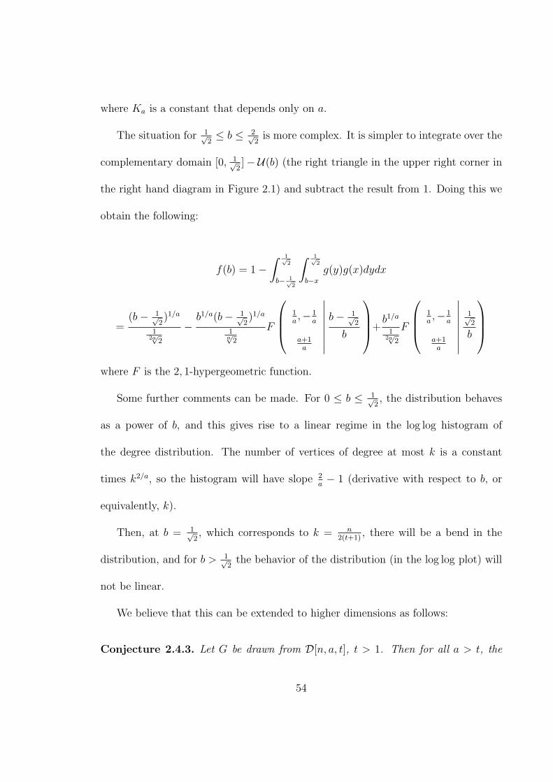
where Ka is a constant that depends only on a.
The situation for 1√2≤ b ≤ 2√
2is more complex. It is simpler to integrate over the
complementary domain [0, 1√2]−U(b) (the right triangle in the upper right corner in
the right hand diagram in Figure 2.1) and subtract the result from 1. Doing this we
obtain the following:
f(b) = 1−∫ 1√
2
b− 1√2
∫ 1√2
b−x
g(y)g(x)dydx
=(b− 1√
2)1/a
12a√2
−b1/a(b− 1√
2)1/a
1a√2
F
1a,− 1
a
a+1a
∣∣∣∣∣∣∣∣
b− 1√2
b
+
b1/a
12a√2
F
1a,− 1
a
a+1a
∣∣∣∣∣∣∣∣
1√2
b
where F is the 2, 1-hypergeometric function.
Some further comments can be made. For 0 ≤ b ≤ 1√2, the distribution behaves
as a power of b, and this gives rise to a linear regime in the log log histogram of
the degree distribution. The number of vertices of degree at most k is a constant
times k2/a, so the histogram will have slope 2a− 1 (derivative with respect to b, or
equivalently, k).
Then, at b = 1√2, which corresponds to k = n
2(t+1), there will be a bend in the
distribution, and for b > 1√2
the behavior of the distribution (in the log log plot) will
not be linear.
We believe that this can be extended to higher dimensions as follows:
Conjecture 2.4.3. Let G be drawn from D[n, a, t], t > 1. Then for all a > t, the
54

log-log plot of the degree distribution of G
• obeys the power law for degrees k ∈ [1, n(a+1)t
] and will have slope t−aa
and
• has an initial bend in the plot occurring at the degree k = n(a+1)t
.
55

Chapter 3
The Sparse Model
In this chapter we present the Sparse Random Dot Product Graph. We begin by
introducing the model and proving basic results in Section 3.1.1. The main results
parallel those in the dense case and are presented in Section 3.2. In Section 3.2.2 we
show that the degree distribution obeys a power law. In Section 3.2.3 we show that
the Sparse Random Dot Product graph has a small diameter. Additionally, unlike the
dense model in which all small subgraphs appear with probability tending to one, in
the sparse model subgraphs appear at certain thresholds dependent upon a parameter
b that is not used in the dense model. In Sections 3.1.1 and 3.1.3 we present specific
results regarding the thresholds for the appearance of edges, cliques, cycles, and trees.
Then in Section 3.2.1, we prove a general threshold result for the appearance of any
fixed graph H. Finally, in Section 3.3 we recap our results, discuss the evolution of
the Sparse Random Dot Product Graph as b goes from zero to infinity.
56

3.1 The Sparse Random Dot Product Graph
In this chapter, we investigate a version of the Random Dot Product Graph in
which the probability mapping f is not the identity function. Instead let f(r) = rnb
where b is a positive1 real number. We denote this sample space of Sparse Random
Dot Product Graphs on n vertices in which one dimensional vectors are drawn from
Ua[0, 1] (a > 1) and for which the probability mapping is f(r) = rnb as DS[n, a, b, 1].
3.1.1 Results in the General Case: b ∈ (0,∞)
We begin by studying the model for the general case when b ∈ (0,∞). We have
the following basic results.
Proposition 3.1.1. Let G be drawn from DS[n, a, b, 1] with b ∈ (0,∞). For any
u, v ∈ V (G) we have
P [u ∼ v] =1
nb (a + 1)2.
Proof:
P [u ∼ v] =
∫ 1
0
∫ 1
0
xu xv
nbg(xu) g(xv) dxu dxv =
1
nb a2
∫ 1
0
∫ 1
0
x1/au x1/a
v dxu dxv
=1
nb (a + 1)2.
1Note that the case b = 0 is the model discussed in Chapter 2.
57

QED.
Thus, an arbitrary edge appears in the graph with probability 1nb (a+1)2
and the
expected number of edges is(
n2
)1
nb (a+1)2³ n2−b
(a+1)2. We would like to know for which
values of b does a Sparse Random Dot Product Graph have edges (with high proba-
bility) and so first we calculate the variance on the number of edges.
Lemma 3.1.2. Let G be drawn from DS[n, a, b, 1] with b ∈ (0,∞). Let the random
variable X be the number of edges in G. Then
Var[X] =
(n2
)
nb(a + 1)2+
6(
n3
)
n2b(1 + 2a)(a + 1)2+
(n2
)(n−2
2
)
n2b(a + 1)4−
(n2
)2
n2b(a + 1)4.
Proof:
Consider X as the sum of the indicator functions for each individual edge. So,
X =∑
u,v∈V (G)u<v
I {u ∼ v}. Therefore by Proposition 3.1.1 we have that
E[X] = E
∑
u,v∈V (G)u<v
I{u ∼ v}
=
∑
u,v∈V (G)u<v
E[ I{u ∼ v}] =∑
u,v∈V (G)u<v
P [u ∼ v] =
(n2
)
nb(a + 1)2.
The variance of X is
Var[X] = E[X2]− E[X]2 = E[X2]−( (
n2
)
nb(a + 1)2
)2
and so we calculate E[X2].
58

E[X2] = E
∑
u,v∈V (G)u<v
I {u ∼ v}
2
= E
∑
u,v∈V (G)u<v
I2 {u ∼ v} +∑
u,v,w∈V (G)u6=v,u 6=w,v 6=w
I {u ∼ v} I {v ∼ w}
+∑
u,v,w,z∈V (G)u<v,w<z,{u,v}∩{w,z}=∅
I {u ∼ v} I {w ∼ z}
= E
∑
u,v∈V (G)u<v
I2 {u ∼ v}
+ E
∑
u,v,w∈V (G)u6=v,u 6=w,v 6=w
I {u ∼ v} I {v ∼ w}
+ E
∑
u,v,w,z∈V (G)u<v,w<z,{u,v}∩{w,z}=∅
I {u ∼ v} I {w ∼ z}
.
We now look at each of the three expected values individually. In the first expected
value, since the indicator random variables can only have the value of 0 or 1 we see
that
E
∑
u,v∈V (G)u<v
I2 {u ∼ v}
= E
∑
u,v∈V (G)u<v
I {u ∼ v}
=
∑
u,v∈V (G)u<v
E [ I {u ∼ v}]
=
(n
2
)P [u ∼ v] =
(n2
)
nb(a + 1)2= E[X].
59

Next, for the middle term, we have that
E
∑
u,v,w∈V (G)u6=v,u 6=w,v 6=w
I {u ∼ v} I {v ∼ w}
=
∑
u,v,w∈V (G)u6=v,u 6=w,v 6=w
E [I {u ∼ v} I {v ∼ w}]
= 6
(n
3
)E [I {u ∼ v} I {v ∼ w}] .
Now, I {u ∼ v} I {v ∼ w} = 1 if and only if I {u ∼ v} = 1 and I {v ∼ w} = 1, and
is 0 otherwise. Therefore,
E [I {u ∼ v} I {v ∼ w}] = P [u ∼ v ∼ w] =
∫ 1
0
∫ 1
0
∫ 1
0
xau xa
v
nb
xav xa
w
nbdxu dxv dxw
=1
n2b(1 + 2a)(1 + a)2.
Hence the middle term is
E
∑
u,v,w∈V (G)u6=v,u 6=w,v 6=w
I {u ∼ v} I {v ∼ w}
=
6(
n3
)
n2b(1 + 2a)(1 + a)2.
Finally, since the events {u ∼ v} and {w ∼ z} are independent, the last term
becomes
E
∑
u,v,w,z∈V (G)u<v,w<z
{u,v}∩{w,z}=∅
I {u ∼ v} I {w ∼ z}
=∑
u,v,w,z∈V (G)u<v,w<z
{u,v}∩{w,z}=∅
E [I {u ∼ v}] E [I {w ∼ z}]
60
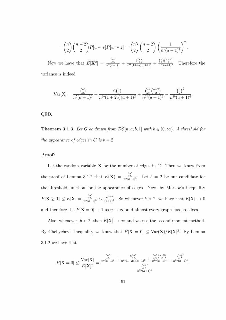
=
(n
2
)(n− 2
2
)P [u ∼ v]P [w ∼ z] =
(n
2
)(n− 2
2
) (1
nb(a + 1)2
)2
.
Now we have that E[X2] =(n
2)nb(a+1)2
+6(n
3)n2b(1+2a)(a+1)2
+(n
2)(n−2
2 )n2b(a+1)4
. Therefore the
variance is indeed
Var[X] =
(n2
)
nb(a + 1)2+
6(
n3
)
n2b(1 + 2a)(a + 1)2+
(n2
)(n−2
2
)
n2b(a + 1)4−
(n2
)2
n2b(a + 1)4.
QED.
Theorem 3.1.3. Let G be drawn from DS[n, a, b, 1] with b ∈ (0,∞). A threshold for
the appearance of edges in G is b = 2.
Proof:
Let the random variable X be the number of edges in G. Then we know from
the proof of Lemma 3.1.2 that E(X) =(n
2)nb(a+1)2
. Let b = 2 be our candidate for
the threshold function for the appearance of edges. Now, by Markov’s inequality
P [X ≥ 1] ≤ E[X] =(n
2)nb(a+1)2
∼ n2−b
(a+1)2. So whenever b > 2, we have that E[X] → 0
and therefore the P [X = 0] → 1 as n →∞ and almost every graph has no edges.
Also, whenever, b < 2, then E[X] → ∞ and we use the second moment method.
By Chebychev’s inequality we know that P [X = 0] ≤ Var(X)/E[X]2. By Lemma
3.1.2 we have that
P [X = 0] ≤ Var[X]
E[X]2=
(n2)
nb(a+1)2+
6(n3)
n2b(1+2a)(a+1)2+
(n2)(
n−22 )
n2b(a+1)4− (n
2)2
n2b(a+1)4
(n2)
2
n2b(a+1)4
.
61

Now let us look at each piece of the fraction separately. The first term is
(n2)
nb(a+1)2
(n2)
2
n2b(a+1)4
∼ n2n2b(a + 1)4
n2nb(a + 1)2=
nb(a + 1)2
n2→ 0
since b < 2. Similarly the second term is
6(n3)
n2b(1+2a)(a+1)2
(n2)
2
n2b(a+1)4
∼ 6 n3n2b(a + 1)4
n4n2b(1 + 2a)(1 + a)2→ 0.
Finally the last term is(n
2)(n−2
2 )n2b(a+1)4
− (n2)
2
n2b(a+1)4
(n2)
2
n2b(a+1)4
< 0.
Therefore P [X = 0] → 0 whenever b < 2 and so b = 2 is a threshold for the
appearance of edges.
QED.
So, the threshold for the appearance of edges is b = 2 or when the probability
mapping is f(r) = rn2 . Therefore whenever b ∈ (2,∞) a Sparse Random Dot Product
Graph is almost surely edgeless. It is interesting to note that 1/n2 is a threshold func-
tion for the appearance of edges in a Erdos-Renyi random graph. Next we examine
the threshold for the appearance of a clique of size k ≥ 2.
Proposition 3.1.4. Let G be drawn from DS[n, a, b, 1] with b ∈ (0,∞). Let k ∈
N, k > 1. For any distinct u1, u2, . . . , uk ∈ V (G) we have that the probability G has a
62

clique of size k on u1, u2, . . . , uk is
P [Kk on u1, u2, . . . , uk] =(1 + (k − 1)a)−k
n(k2)b
.
Proof:
P [Kk on u1, u2, . . . , uk] =
∫ 1
0
· · ·∫ 1
0
xu1 xu2
nb
xu1 xu3
nb· · · xu1 xuk
nb· · · xuk−1
xuk
nb
g(xu1) g(xu2) · · · g(xuk) dxu1 dxu2 · · · dxuk
=1
n(k2)b
∫ 1
0
· · ·∫ 1
0
xk−1u1
xk−1u2
· · ·xk−1uk
g(xu1) g(xu2) · · · g(xuk) dxu1 dxu2 · · · dxuk
=1
n(k2)b
[∫ 1
0
xk−1ui
g(xui)dxui
]k
=(1 + (k − 1)a)−k
n(k2)b
.
QED.
Therefore the expected number of cliques of size k is(
nk
) (1+(k−1)a)−k
n(k2)b
.
Theorem 3.1.5. Let G be drawn from DS[n, a, b, 1] with b ∈ (0,∞). Let k ∈ N, k >
1. A threshold for the appearance of cliques of size k is b = 2k−1
.
Proof:
Let the random variable X be the number of cliques of size k in G. Then we know
by Proposition 3.1.4 that E(X) =(
nk
) (1+(k−1)a)−k
n(k2)b
. Let b = 2k−1
be our candidate for
63

the threshold for the appearance of Kk. Now, by Markov’s inequality
P [X ≥ 1] ≤ E[X] =
(n
k
)(1 + (k − 1)a)−k
n(k2)b
∼ nk− k(k−1)2
b
(1 + (k − 1)a)k.
So whenever b > 2k−1
, we have that E[X] → 0 and therefore the P [X = 0] → 1 as
n →∞ and almost every graph has no clique of size k.
Also, whenever, b < 2k−1
, then E[X] → ∞ and we apply the second moment
method. By Chebychev’s inequality we know that P [X = 0] ≤ Var(X)/E[X]2.
Let Iu1,u2,...,ukbe the indicator function for when the vertices u1, u2, . . . , uk are a
clique. Then X =∑
u1<u2<···<ukIu1,u2,...,uk
. The variance of X is
Var[X] = E[X2]− E[X]2 = E[X2]−[(
n
k
)(1 + (k − 1)a)−k
n(k2)b
]2
and so we calculate E[X2].
E[X2] = E
( ∑u1<u2<···<uk
Iu1,u2,...,uk
)2
= E
[( ∑u1<u2<···<uk
Iu1,u2,...,uk
)( ∑y1<y2<···<yk
Iy1,y2,...,yk
)]
=∑
u1<u2<···<uky1<y2<···<yk
E[Iu1,u2,...,ukIy1,y2,...,yk
].
Now in each term of the summation u1, . . . , uk and y1, . . . yk overlap in up to k
terms. Let {z1, z2, . . . , zk+j} = {u1, . . . , uk, y1, . . . yk} then u1, . . . , uk and y1, . . . yk
64

overlap in exactly 2k− (k + j) = k− j terms, for some j with 0 ≤ j ≤ k, and we can
rewrite the summation as
E[X2] =k∑
j=0
∑u1<u2<···<uky1<y2<···<yk
|{u1,...,uk,y1,...yk}|=k+j
E[Iu1,u2,...,ukIy1,y2,...,yk
]
=k∑
j=0
∑u1<u2<···<uky1<y2<···<yk
|{u1,...,uk,y1,...yk}|=k+j
P [u1, u2, . . . , uk is a clique and y1, . . . , yk is a clique].
Let us consider this probability for a moment. In this integral, each edge ap-
pears only once, regardless if it occurs in both cliques. Therefore there are exactly
2(
k2
) − (k−j2
)edges each contributing a 1
nb term to the integral. Also, without loss
of generality, let us assume that z1, . . . , zk−j are the vertices that overlap, i.e. they
appear in both cliques. Therefore, they each appear in exactly k− 1 + j edges, while
the remaining vertices appear in only k− 1 edges. Hence, their vectors, xz1 , . . . , xzk−j
appear in the integral k − 1 + j times and the vectors xzk−j+1, . . . xzk+j
appear k − 1
times. So we see that the probability is
P [u1, u2, . . . , uk is a clique and y1, . . . , yk is a clique] =
=1
n[2(k2)−(k−j
2 )]b
∫ 1
0
· · ·∫ 1
0
xa(k+j−1)z1
· · ·xa(k+j−1)zk−j
xa(k−1)zk−j+1
· · ·xa(k−1)zk+j
dxz1 · · · dxzk+j
65

which by separating the integrals and collecting like terms becomes
=1
n[2(k2)−(k−j
2 )]b
[∫ 1
0
xa(k−1)zk−j+1
dxzk−j+1
]2j [∫ 1
0
xa(k−1+j)z1
dxz1
]k−j
=1
n[2(k2)−(k−j
2 )]b
[1
a(k − 1) + 1
]2k [1
a(k − 1 + j) + 1
]k−j
.
So, we see that our equation becomes
E[X2] =k∑
j=0
∑u1<u2<···<uky1<y2<···<yk
|{u1,...,uk,y1,...yk}|=k+j
1
n[2(k2)−(k−j
2 )]b
[1
a(k − 1) + 1
]2j [1
a(k − 1 + j) + 1
]k−j
=k∑
j=0
(k
k−j
)(nk
)(n−k
j
)
n[2(k2)−(k−j
2 )]b1
(a(k − 1) + 1)2j
1
(a(k − 1 + j) + 1)k−j.
We can now write the variance in more detail and in Chebychev’s inequality we
now have that
P [X = 0] ≤ Var[X]
E[X]2=
∑kj=0
( kk−j)(
nk)(
n−kj )
n[2(k2)−(k−j
2 )]b1
(a(k−1)+1)2j1
(a(k−1+j)+1)k−j − E[X]2
E[X]2.
We claim that the above value is going to 0 as n →∞. We show this by considering
the righthand side of the inequality in three parts and showing that each of the parts
individually goes to zero or is negative.
66

First we note that when j = 0 each of the ui = yi, 1 ≤ i ≤ k, and the value is
(nk
)
n(k2)b
1
(a(k − 1) + 1)k= E[X].
Therefore in the Chebychev’s we have that as n →∞
(nk)
n(k2)b
1(a(k−1)+1)k
E[X]2=
E[X]
E[X]2→ 0.
Next when j = k and none of the terms overlap the value is
(nk
)(n−k
k
)1
(a(k−1)+1)2k
n2(k2)b
< E[X]2.
Therefore in the Chebychev’s inequality we have that as n →∞
(nk)(
n−kk ) 1
(a(k−1)+1)2k
n2(k
2)b− E[X]2
E[X]< 0.
So, consider any j, 1 ≤ j ≤ k − 1. Then the term in the summation is
( kk−j)(
nk)(
n−kj )
n[2(k2)−(k−j
2 )]b1
(a(k−1)+1)2j1
(a(k−1+j)+1)k−j
E[X]2=
( kk−j)(
nk)(
n−kj )
n[2(k2)−(k−j
2 )]b1
(a(k−1)+1)2j1
(a(k−1+j)+1)k−j
(nk)
2
n2(k
2)b
1(a(k−1)+1)k
67

which for fixed k is
³ nknj
n[2(k2)−(k−j
2 )]b
n2(k2)b
n2k
(a(k − 1) + 1)k−2j
(a(k − 1 + j) + 1)k−j
= C(a, k, b, j)/nk−j−(k−j2 )b
and is simply a constant, that does not depend on n, times 1/nk−j−(k−j2 )b. Whenever
b < 2k−1
we have that the power on n is
k − j −(
k − j
2
)b > k − j −
(k − j
2
)2
k − 1=
j(k − j)
k − 1≥ 1
since 1 ≤ j ≤ k − 1. Therefore whenever 1 ≤ j ≤ k − 1 the term in Chebychev’s
inequality is( k
k−j)(nk)(
n−kj )
n[2(k2)−(k−j
2 )]b1
(a(k−1)+1)2j1
(a(k−1+j)+1)k−j
E[X]2<
1
n→ 0
as n →∞.
Hence, P [X = 0] → 0 as n →∞ and we will almost surely have a clique of size k
whenever b < 2k−1
.
QED.
So, the threshold for the appearance of a clique of size k is b = 2k−1
, i.e., when the
probability mapping is f(r) = rn2/(k−1) which agrees with the threshold function for
the appearance of cliques of size k in a Erdos-Renyi random graph. Therefore when
b < 2k−1
almost every graph will have a clique of size k and whenever b > 2k−1
almost
68

no graph will have a clique of size k, which gives us the following result.
Corollary 3.1.6. Let G be drawn from DS[n, a, b, 1] with b ∈ (0, 2). Let A = { 2i−1
:
i ∈ Z+}. Let kb = max{k : b < 2k−1
, k ∈ Z+}. Then the clique number of G satisfies
ω(G) ∈
{kb, kb + 1} b ∈ A
{kb} b 6∈ A
.
Proof:
First note that since b < 2kb−1
, by Theorem 3.1.5, G will almost surely have a
clique of size kb and so ω(G) ≥ kb.
Now, if b ∈ A, then b = 2kb
= 2(kb+1)−1
. Therefore, ∀k > kb + 1, b > 2k−1
. Hence
by Theorem 3.1.5, G will almost surely not contain a clique of size k. Therefore,
ω(G) ≤ kb + 1.
Similarly, if b 6∈ A, then b > 2kb
= 2(kb+1)−1
and so again by Theorem 3.1.5, G will
almost surely not contain a clique of size kb + 1. Hence, ω(G) ≤ kb.
QED.
3.1.2 Results when b ∈ (0, 1)
In this section we consider the case when the probability mapping is f(r) = rnb
for b ∈ (0, 1). Assume that n is large. We study the degree distribution of G.
69

Proposition 3.1.7. Let G be drawn from DS[n, a, 1] with b ∈ (0, 1). The expected
number of vertices of degree zero in G is
E[|{v : d(v) = 0}|] ∼(
1
a(1 + a)
1a Γ
(1
a
))n
a−1+ba .
Proof:
Choose v ∈ V (G) fixed, but arbitrary, and denote the vector of v by y. Let
x1, x2, . . . , xn−1 be the vectors of the remaining n− 1 vertices in V (G)− {v}. Then
P [d(v) = 0] =
∫ 1
0
∫ 1
0
· · ·∫ 1
0
(1− x1y
nb) · · · (1− xn−1y
nb)
· g(x1) · · · g(xn−1) g(y) dx1 · · · dxn−1 dy
which is separable. Noting that for each of the xi’s
∫ 1
0
(1− xiy
nb)g(xi)dxi =
∫ 1
0
1
a(1− xiy
nb)x
1−aa
i dxi = 1− y
nb(a + 1)
we have that
P [d(v) = 0] =
∫ 1
0
(1− y
nb(a + 1)
)n−11
ay
1−aa dy.
70
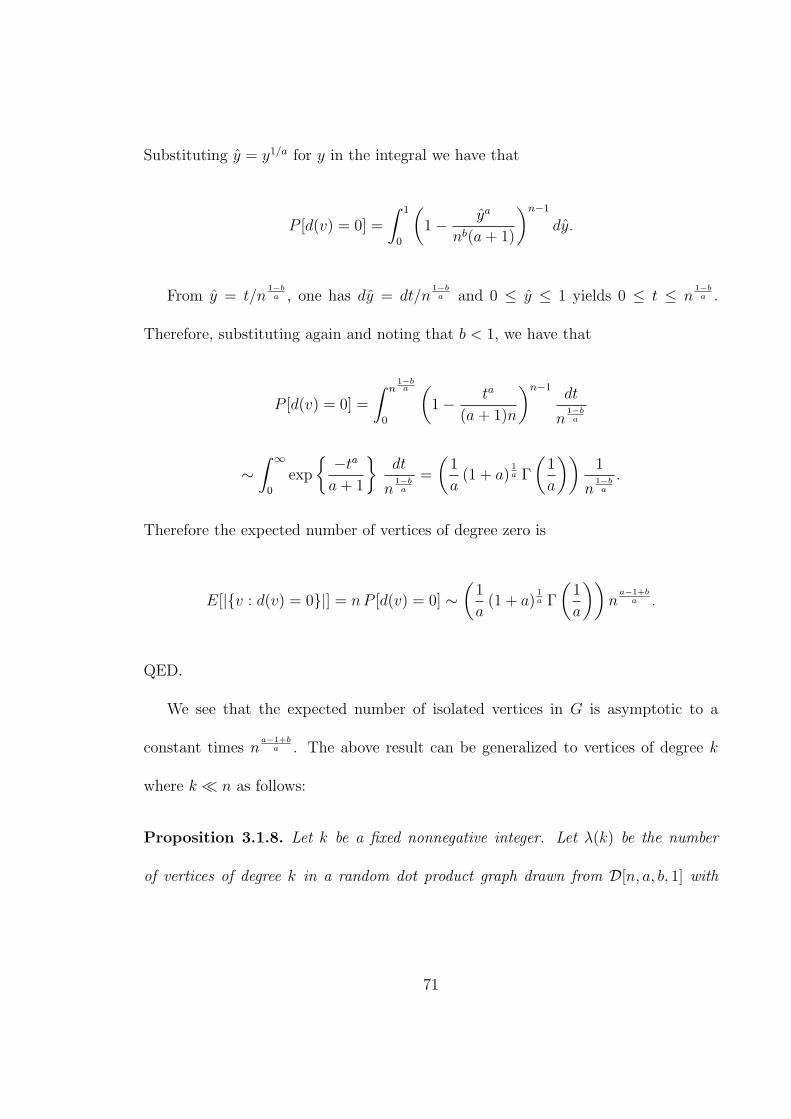
Substituting y = y1/a for y in the integral we have that
P [d(v) = 0] =
∫ 1
0
(1− ya
nb(a + 1)
)n−1
dy.
From y = t/n1−b
a , one has dy = dt/n1−b
a and 0 ≤ y ≤ 1 yields 0 ≤ t ≤ n1−b
a .
Therefore, substituting again and noting that b < 1, we have that
P [d(v) = 0] =
∫ n1−b
a
0
(1− ta
(a + 1)n
)n−1dt
n1−b
a
∼∫ ∞
0
exp
{ −ta
a + 1
}dt
n1−b
a
=
(1
a(1 + a)
1a Γ
(1
a
))1
n1−b
a
.
Therefore the expected number of vertices of degree zero is
E[|{v : d(v) = 0}|] = nP [d(v) = 0] ∼(
1
a(1 + a)
1a Γ
(1
a
))n
a−1+ba .
QED.
We see that the expected number of isolated vertices in G is asymptotic to a
constant times na−1+b
a . The above result can be generalized to vertices of degree k
where k ¿ n as follows:
Proposition 3.1.8. Let k be a fixed nonnegative integer. Let λ(k) be the number
of vertices of degree k in a random dot product graph drawn from D[n, a, b, 1] with
71

b ∈ (0, 1). Then
E[λ(k)] ∼(
1
k! a(1 + a)
1a Γ
(1
a+ k
))n
a−1+ba
as n →∞.
In the dense version of the Random Dot Product Graph we discussed the idea of
clustering in Section 2.3.2. This property clearly distinguishes the dense version of
the model from an Erdos-Renyi random graph which does not exhibit any clustering.
We have an analogous result for the Sparse Random Dot Product Graph.
Proposition 3.1.9. Let G be drawn from DS[n, a, b, 1] with b ∈ (0, 1). Let v ∈ V (G)
and let N(v) be the open neighborhood of v. Then ∀u,w ∈ N(v),
P [u ∼ w|u ∼ v ∼ w] =(a + 1)2
nb(2a + 1)2.
Note the proof is almost identical to that of Lemma 2.3.6 and is therefore omitted.
While it is true that for any vertices u, v, and w, the P [u ∼ v] < P [u ∼ v|u ∼
w ∼ v] and so some clustering does exist, we see that P [u ∼ v|u ∼ w ∼ v] − P [u ∼
v] = (1+a)2
nb(1+2a)2− 1
nb(a+1)2→ 0 as n → ∞. So, in the Sparse Random Dot Product
Graph we cannot use clustering as an example of a limiting behavior different from
that of an Erdos-Renyi random graph.
It is well known that log nn
is a threshold function for the disappearance of isolated
72

vertices in an Erdos-Renyi random graph. We will show that in the Sparse Random
Dot Product Graph no such threshold exists.
Proposition 3.1.10. Let G be drawn from DS[n, a, b, 1] with b ∈ (0, 1). For each
vertex v ∈ V (G), let Xv be the indicator that v is isolated. Let X =∑
v∈V (G) Xv be
the number of isolated vertices in G. Then P [X > 0] → 1 as n → ∞ and almost
every graph has isolated vertices.
Proof:
First recall from Proposition 3.1.7 that E[X] ∼(
1a(1 + a)
1a Γ
(1a
))n
a−1+ba → ∞
for all b ∈ (0, 1). Also, by Chebychev’s inequality we know that P [X = 0] ≤
Var(X)/E[X]2 = E[X2]−E[X]2
E[X]2and so we calculate E[X2].
E[X2] = E
∑
v∈V (G)
Xv
2
(where Xv is the indicator that v is isolated)
= E
∑
v∈V (G)
Xv
∑
u∈V (G)
Xu
=∑
u,v∈V (G)
E[XuXv].
If u = v then XuXv = Xv and so we have that
E[X2] =∑
v∈V (G)
E[Xv] +∑
u,v∈V (G):u6=v
E[XuXv]
73

= E[X] + 2
(n
2
)P [u and v are both isolated].
Now, u, v ∈ V (G) with vectors x and y, respectively. Let x1, x2, . . . , xn−2 be the
vectors of the remaining n− 2 vertices in V (G)− {u, v}. Then
P [u and v are both isolated] =
=
∫ 1
0
∫ 1
0
· · ·∫ 1
0
(1− xy
nb)((1− x1x
nb)(1− x1y
nb))· · ·
((1− xn−2x
nb)(1− xn−2y
nb))
·g(x1) · · · g(xn−1) g(y) dx1 · · · dxn−2 dx dy
which is separable. Noting that for each of the xi’s
∫ 1
0
(1− xix
nb)(1− xiy
nb)g(xi)dxi = 1− x
nb(a + 1)− y
nb(a + 1)+
xy
n2b(2a + 1)
we have that
P [u and v are both isolated] =
=
∫ 1
0
∫ 1
0
(1− xy
nb)
(1− x
nb(a + 1)− y
nb(a + 1)+
xy
n2b(2a + 1)
)n−21
ax
1−aa
1
ay
1−aa dx dy
and substituting x = x1/a and y = y1/a for y in the integral we have that
=
∫ 1
0
∫ 1
0
(1− xaya
nb)
(1− xa
nb(a + 1)− ya
nb(a + 1)+
xaya
n2b(2a + 1)
)n−2
dx dy
74

≤∫ 1
0
∫ 1
0
(1− xa
nb(a + 1)− ya
nb(a + 1)+
xaya
n2b(2a + 1)
)n−2
dx dy
(since (1− xaya
nb ) ≤ 1)
≤∫ 1
0
∫ 1
0
exp
[−(n− 2)
(xa
nb(a + 1)+
ya
nb(a + 1)− xaya
n2b(2a + 1)
)]dx dy
=
∫ 1
0
exp
[−(n− 2)
(xa
nb(a + 1)
)]
·∫ 1
0
exp
[−(n− 2)
(ya
nb(a + 1)− xaya
n2b(2a + 1)
)]dx dy
≤∫ 1
0
exp
[−(n− 2)
(xa
nb(a + 1)
)]
·∫ ∞
0
exp
[−(n− 2)
(ya
nb(a + 1)− xaya
n2b(2a + 1)
)]dx dy
=
∫ 1
0
exp
[−(n− 2)
(xa
nb(a + 1)
)]
·(
1
aΓ(
1
a)
[(n− 2)
(1
nb(a + 1)− xa
n2b(2a + 1)
)]− 1a
)dx
≤∫ 1
0
exp
[−(n− 2)
(xa
nb(a + 1)
)]
·(
1
aΓ(
1
a)
[(n− 2)
(1
nb(a + 1)− 1
n2b(2a + 1)
)]− 1a
)dx
(since xa ≤ 1)
75

≤(
1
aΓ(
1
a)
[(n− 2)
(1
nb(a + 1)− 1
n2b(2a + 1)
)]− 1a
)
·∫ ∞
0
exp
[−(n− 2)
(xa
nb(a + 1)
)]dx
=
(1
aΓ(
1
a)
[(n− 2)
(1
nb(a + 1)− 1
n2b(2a + 1)
)]− 1a
)
·(
1
aΓ(
1
a)
[(n− 2)
(1
nb(a + 1)
)]− 1a
)
=
(1
aΓ(
1
a)
)2
(n− 2)−2a
[(1
nb(a + 1)− 1
n2b(2a + 1)
)(1
nb(a + 1)
)]− 1a
.
So, we have that
E[X2] ≤ E[X]
+2
(n
2
) (1
aΓ(
1
a)
)2
(n− 2)−2a
[(1
nb(a + 1)− 1
n2b(2a + 1)
)(1
nb(a + 1)
)]− 1a
.
Hence
P [X = 0] ≤ E[X2]− E[X]2
E[X]2
≤E[X] + 2
(n2
) (1aΓ( 1
a))2
(n− 2)−2a
[(1
nb(a+1)− 1
n2b(2a+1)
)(1
nb(a+1)
)]− 1a − E[X]2
E[X]2
∼ E[X]
E[X]2+
(1aΓ( 1
a))2
n2− 2a
[(1
nb(a+1)− 1
n2b(2a+1)
)(1
nb(a+1)
)]− 1a
E[X]2− E[X]2
E[X]2.
76

Now, E[X]E[X]2
→ 0 as n →∞ and E[X]2
E[X]2= 1. Also,
(1aΓ( 1
a))2
n2− 2a
[(1
nb(a+1)− 1
n2b(2a+1)
)(1
nb(a+1)
)]− 1a
E[X]2∼
∼(
1aΓ( 1
a))2
n2− 2a
[(1
nb(a+1)− 1
n2b(2a+1)
) (1
nb(a+1)
)]− 1a
((1a(1 + a)
1a Γ
(1a
))n1− 1
a+ b
a
)2
=
(1
nb(a+1)− 1
n2b(2a+1)
)− 1a
(1 + a)1a n
ba
=
(n2b(a+1)(2a+1)nb(2a+1)−(a+1)
) 1a
(1 + a)1a n
ba
=
(nb(2a + 1)
nb(2a + 1)− (a + 1)
) 1a
→ 1
as n →∞. Therefore
P [X = 0] → 0 + 1− 1 = 0
as n →∞ and almost every graph contains isolated vertices.
QED.
77

3.1.3 The Land of Trees: b ∈ (1, 2)
In this section we discuss the behavior of the Sparse Random Dot Product Graph
when the parameter b ∈ (1, 2). With this restriction on b, the graph will, with high
probability, contain no cycles and therefore be a forest on trees of size bb−1
or less.
For any graph H, let P≥[H] be the probability of H appearing as a (not necessarily
induced) subgraph of a Sparse Random Dot Product Graph G on a specific set of
vertices in a specific order. We begin by showing a general result relating the number
of edges in a graph H to P≥[H].
Proposition 3.1.11. Let G be drawn from DS[n, a, b, 1] with b ∈ (0,∞). Let H be a
graph on k > 1 vertices with m ≥ 1 edges. For any distinct u1, u2, . . . , uk ∈ V (G) we
have that the probability of H appearing with edges e1, e2, . . . em on u1, u2, . . . , uk is
P≥[H on u1, u2, . . . , uk] =C(H)
nm b
where C(H) is a constant that depends on the graph H and does not vary with n or
b.
Proof:
Let H be a graph on the k vertices u1, u2, . . . , uk with edges e1, e2, . . . , em. Let us
assume that each ei ∈ E(H) has endpoints l(ei) and r(ei) with vectors x(ei) and y(ei),
respectively, where l(ei), r(ei) ∈ {u1, u2, . . . , uk} and x(ei), y(ei) ∈ {xu1 , xu2 , . . . , xuk}.
Also for each 1 ≤ i ≤ k, let ri be the number of edges incident to ui. Then
78

P≥[H on u1, u2, . . . , uk] =
∫ 1
0
· · ·∫ 1
0
x(e1) y(e1)
nb
x(e2) y(e2)
nb· · · x(em) y(em)
nb
g(xu1) g(xu2) · · · g(xuk) dxu1 dxu2 · · · dxuk
=1
nm b
∫ 1
0
· · ·∫ 1
0
xr1u1
xr2u2· · · xrk
ukg(xu1) g(xu2) · · · g(xuk
) dxu1 dxu2 · · · dxuk
=1
nm b
(∫ 1
0
xr1u1
g(xu1) dxu1
)(∫ 1
0
xr2u2
g(xu2) dxu2
)· · ·
(∫ 1
0
xrkuk
g(xuk) dxuk
)
=1
nm b
(1
ar1 + 1
)(1
ar2 + 1
)· · ·
(1
ark + 1
)
=C(H)
nm b
where C(H) =(
1ar1+1
)(1
ar2+1
)· · ·
(1
ark+1
)and does not vary with n or b. One should
note that this probability is essentially a constant over n raised to the number of edges
in the graph times b.
QED.
So, for trees we have the following result.
Corollary 3.1.12. Let G be drawn from DS[n, a, b, 1] with b ∈ (0,∞). Let k ∈ N, k >
1. For any distinct u1, u2, . . . , uk ∈ V (G) we have that the probability of T appearing
with k − 1 edges e1, e2, . . . em on u1, u2, . . . , uk is
P≥[T on u1, u2, . . . , uk] =C(H)
n(k−1) b
79

where C(T ) is a constant that depends on the tree T and does not vary with n or b.
Therefore the expected number of copies of a tree T is E[T ] ³ (nk)
n(k−1)b ³ nk−(k−1)b
and so if b > kk−1
then we do not expect to see the tree T .
Theorem 3.1.13. Let G be drawn from DS[n, a, b, 1] with b ∈ (0,∞). Let k ∈ Z+.
A threshold for the appearance of a tree on k vertices is b = kk−1
.
Proof:
Let T be a tree on k vertices. Let the random variable X be the number of copies
of T in G. Then we know by Corollary 3.1.12 that E(X) ³ nk−(k−1)b. Let b = kk−1
be
our candidate for the threshold for the appearance of T . Now, by Markov’s inequality
P [X ≥ 1] ≤ E[X] ³ nk−(k−1)b.
So whenever b > kk−1
, we have that E[X] → 0 and therefore the P [X = 0] → 1 as
n →∞ and almost no graph contains a copy of T .
Also, whenever, b < kk−1
, then E[X] → ∞ and we apply the second moment
method. By Chebychev’s inequality we know that P [X = 0] ≤ Var(X)/E[X]2.
Let T be the set of all copies of T possible on V (G). For any T ′ ∈ T , let IT ′ be
the indicator function for the specific copy T ′, then X =∑
T ′∈T IT ′ . The variance of
X is
Var[X] = E[X2]− E[X]2 ³ E[X2]− [nk−(k−1)b
]2
80

and so we calculate E[X2].
E[X2] = E
(∑
T ′∈TIT ′
)2
= E
[(∑
T ′∈TIT ′
)( ∑
T ′′∈TIT ′′
)]
=∑
T ′,T ′′∈TE[IT ′IT ′′ ].
Now in each term of the summation T ′ and T ′′ share up to k − 1 edges and we
can rewrite the summation as
E[X2] =k−1∑i=0
∑
T ′,T ′′∈T|E(T ′)∩E(T ′′)|=i
E[IT ′IT ′′ ]
=k−1∑i=0
∑
T ′,T ′′∈T|E(T ′)∩E(T ′′)|=i
E[IT ′IT ′′ ]
=k−1∑i=0
∑
T ′,T ′′∈T|E(T ′)∩E(T ′′)|=i
P≥[T ′ ∪ T ′′].
Now, by a discussion similar to that in the proof of Proposition 3.1.12 it can be
seen that
P≥[T ′ ∪ T ′′] =C(T ′, T ′′)
n(|E(T ′)∪E(T ′′)|)b =C(T ′, T ′′)n(2(k−1)−i)b
where i is the number of edges that T and T ′′ share and C(T ′, T ′′) is a constant, not
81
dependent on n or b. Hence, we have that
E[X2] =k−1∑i=0
∑
T ′,T ′′∈T|E(T ′)∩E(T ′′)|=i
C(T ′, T ′′)n(2(k−1)−i)b
=∑
T ′,T ′′∈T|E(T ′)∩E(T ′′)|=0
C(T ′, T ′′)n2(k−1)b
+k−1∑i=1
∑
T ′,T ′′∈T|E(T ′)∩E(T ′′)|=i
C(T ′, T ′′)n(2(k−1)−i)b
.
If T and T ′′ share i > 1 edges, then they also share at least i + 1 vertices and
so for each i > 1 we have at no more than(
n2k−(i+1)
)cT possible choices for the pair
(T ′, T ′′), where cT depends only on T and is a constant with respect to n and b. So
we have that
E[X2] ≤∑
T ′,T ′′∈T|E(T ′)∩E(T ′′)|=0
C(T ′, T ′′)n2(k−1)b
+k−1∑i=1
(n
2k − (i + 1)
)cT
C(T ′, T ′′)n(2(k−1)−i)b
.
Now, returning to Chebychev’s inequality we have that
P [X = 0] ≤ Var(X)
E[X]2=
E[X2]− E[X]2
E[X]2
≤
∑T ′,T ′′∈T
|E(T ′)∩E(T ′′)|=0
C(T ′,T ′′)n2(k−1)b +
∑k−1i=1
(n
2k−(i+1)
)cT
C(T ′,T ′′)n(2(k−1)−i)b − E[X]2
E[X]2
³
∑
T ′,T ′′∈T|E(T ′)∩E(T ′′)|=0
1
n2(k−1)b+
k−1∑i=1
n2k−(i+1)
n(2(k−1)−i)b− (
nk−(k−1)b)2
1
(nk−(k−1)b)2
82

=
(∑T ′,T ′′∈T
|E(T ′)∩E(T ′′)|=0
1n2(k−1)b
)− (
nk−(k−1)b)2
(nk−(k−1)b)2 +
∑k−1i=1
n2k−(i+1)
n(2(k−1)−i)b
(nk−(k−1)b)2 .
We will examine the first term of the summation separately from the remaining
terms. In the first term, any pair, T ′ and T ′′, share no edges, but may share vertices.
Let us assume that they share j ∈ {0, k} vertices, then the term can be written as
∑k
j=0
∑T ′,T ′′∈T
|E(T ′)∩E(T ′′)|=0|V (T ′)∩V (T ′′)|=j
1n2(k−1)b
− (
nk−(k−1)b)2
(nk−(k−1)b)2
(and is less than)
≤
(∑kj=0
(nk)(
n−kk−j)2k!
n2(k−1)b
)− (
nk−(k−1)b)2
(nk−(k−1)b)2
(which for large n is)
≤
(∑kj=0
(nk)(
n−kk )2k!
n2(k−1)b
)− (
nk−(k−1)b)2
(nk−(k−1)b)2
=
((k + 1)
(nk)(
n−kk )2k!
n2(k−1)b
)− (
nk−(k−1)b)2
(nk−(k−1)b)2
³nk(n−k)k
n2(k−1)b − nknk
n2(k−1)b
(nk−(k−1)b)2
< 0.
83

So, the first term in the summation is less than zero and we only need to consider
the remaining terms and so we have that
P [X = 0] ³
(∑T ′,T ′′∈T
|E(T ′)∩E(T ′′)|=0
1n2(k−1)b
)− (
nk−(k−1)b)2
(nk−(k−1)b)2 +
∑k−1i=1
n2k−(i+1)
n(2(k−1)−i)b
(nk−(k−1)b)2
< 0 +k−1∑i=1
n2k−(i+1)
n(2(k−1)−i)b
(nk−(k−1)b)2 =
k−1∑i=1
n−(i+1)−i b.
Now, if for each i ∈ {1, k − 1} we can show that b < i+1i
, then P [X = 0] → 0 as
n → ∞. We know that each i ≤ k − 1 and b < kk−1
. Additionally, i+1i
is minimized
when i = k − 1. Thus for all i ∈ {1, k − 1}, i+1i≥ k
k−1> b. Hence, P [X = 0] → 0 as
n →∞ and we will almost surely have a copy of T whenever b < kk−1
.
QED.
So, the threshold for the appearance of a tree on k vertices is b = kk−1
. Therefore
when b < kk−1
almost every graph will have a tree of size k and whenever b > 2k−1
almost no graph will have a clique of size k, which gives us the following result.
Corollary 3.1.14. Let G be drawn from DS[n, a, b, 1] with b ∈ (0,∞). Let k be a
fixed positive integer, then whenever
• b ∈ (0, 1], G will almost surely contain all trees on k or fewer vertices,
• b ∈ (1, 2), G will almost surely contain a tree on k vertices if and only if k < bb−1
,
• b ∈ (2,∞), G will almost surely contain no edges.
84

Proof:
Theorem 3.1.13 we know that with high probability G will contain a tree on k
vertices whenever b < kk−1
. Secondly, for all k ∈ Z+, kk−1
> 1 and thus G will almost
surely contain a tree of size k. Also with high probability, b < kk−1
if and only if
k < bb−1
. So, for all (2,∞), the only positive integer less than bb−1
is 1, and hence
there are no trees on 2 or more vertices. Finally, when b ∈ (1, 2), with high probability
G will contain a tree on k vertices if and only if k < bb−1
.
QED.
Thus far we have shown that whenever b ∈ (1, 2), G will almost surely contain
trees on at most kb = d bb−1e − 1 vertices. We now show that G will almost surely be
without cycles and thus a forest.
Proposition 3.1.15. Let G be drawn from DS[n, a, b, 1] with b ∈ (0,∞). Let k ∈
N, k > 1. For any distinct u1, u2, . . . , uk ∈ V (G) we have that the probability of the
k-cycle u1, u2, . . . , uk, u1 is
P≥[the k-cycle u1, u2, . . . , uk, u1] =(2a + 1)−k
nkb.
Proof:
P≥[the k-cycle u1, u2, . . . , uk, u1] =
∫ 1
0
· · ·∫ 1
0
xu1 xu2
nb
xu2 xu3
nb· · · xuk−1
xuk
nb
xukxu1
nb
g(xu1) g(xu2) · · · g(xuk) dxu1 dxu2 · · · dxuk
85

=1
nkb
∫ 1
0
· · ·∫ 1
0
x2u1
x2u2· · · x2
ukg(xu1) g(xu2) · · · g(xuk
) dxu1 dxu2 · · · dxuk
=1
nkb
[∫ 1
0
x2ui
g(xui)dxui
]k
=(2a + 1)−k
nkb.
QED.
Therefore the expected number of of size k-cycles is(
nk
)(k − 1)! (2a+1)−k
nkb .
Theorem 3.1.16. Let G be drawn from DS[n, a, b, 1] with b ∈ (1, 2). Let kb =
d bb−1e − 1. Then with high probability, G is a forest containing trees with at most kb
vertices.
Proof:
By Corollary 3.1.14, with high probability G will contain trees on 1, 2, . . . , kb
vertices and will not contain trees on kb + 1 or more vertices. Specifically, G will not
contain any path of length kb + 1 or greater. Hence, with high probability, G will
not contain a cycle of length kb + 1 or greater. Let 2 ≤ c ≤ kb, and let the random
variable Xc be the number of cycles of length c in G. Then we know by Proposition
3.1.15 that E(Xc) =(
nc
)(c− 1)! (2a+1)−c
ncb . Now, by Markov’s inequality
P [Xc ≥ 1] ≤ E[Xc] ³ nc(1−b) ≤ nkb(1−b) → 0
as n → ∞ since kb < bb−1
. Hence almost no graph contains a cycle of length c ∈
86

{2, 3, . . . , kb}. Thus with high probability, G will not contain any cycles and hence
will be a forest.
QED.
3.2 Main Results
3.2.1 The Threshold Result
Let H be a graph with k vertices and l ≥ 1 edges. We define ε(H) = lk, i.e., the
number of edges divided by the number of vertices. Also, let
ε′(H) = max{ε(F )|F is a nonempty subgraph of H}.
Then we have the following result about the appearance of any graph H.
Theorem 3.2.1. Let G be drawn from DS[n, a, b, 1] with b ∈ (0,∞). Let H be a graph
with k vertices and l ≥ 1 edges. Then b = 1ε′(H)
is a threshold for the appearance of
H.
Proof:
Let H be the set of all graphs that lie on a subset of the vertex set of G and are
isomorphic to H. Note that |H| = Θ(nk). Also, ∀H ′ ∈ H let XH′ be the indicator
function for when H ′ is a subgraph of G. Let X be number of subgraphs of G that
are isomorphic to H. Then X =∑
H′⊆H XH′ and by linearity of expectation we have
87

that
E[X] =∑
H′⊆HE[XH′ ] = Θ(nk)P≥[H ′].
Let x1, . . . , xk be the vectors of vertices h1, . . . , hk of H ′, respectively. Then
P≥[H ′] =
=
∫ 1
0
· · ·∫ 1
0
∏
1≤i<j≤k
(xixj
nb
)I{hi∼hj in H′}g(x1) · · · g(xk)dx1 · · · dxk
=1
nlb
∫ 1
0
· · ·∫ 1
0
∏
1≤i<j≤k
(xixj)I{hi∼hj in H′}g(x1) · · · g(xk)dx1 · · · dxk
=1
nlbC(H ′, a)
where C(H ′, a) depends only on H ′ and a and is a constant with respect to n and b.
Also, for any H ′, H ′′ ⊆ H, C(H ′, a) = C(H ′′, a) = C(H, a). Hence
E[X] = Θ(nk)1
nlbC(H, a) = Θ(nk−lb).
Let F = (V (F ), E(F )) be a subgraph of H such that ε′(H) = ε(F ) and let
b > 1ε′(H)
. Also, let Y be the number of subgraphs isomorphic to F on G. Then a
discussion similar to that above, E[Y ] = Θ(n|V (F )|−|E(F )|b). Now, b > 1ε′(H)
gives us
that
|V (F )| − |E(F )|b < |V (F )| − |E(F )| 1
ε′(H)
88

= |V (F )| − |E(F )| 1
ε(F )= |V (F )| − |E(F )| |V (F )|
|E(F )| = 0
and so E[Y ] → 0. Hence by Markov’s inequality P [Y > 0] ≤ E[Y ] → 0 and almost
no graph contains F as a subgraph, therefore since F ⊆ H, almost no graph contains
H as a subgraph when b > 1ε′(H)
.
When b < 1ε′(H)
we see that k− lb > k− l 1ε′(H)
> k− l 1ε(H)
= k− l kl
= 0 and hence
E[X] = Θ(nk−lb) → ∞ and we use the second moment method. That is we show
that P [X = 0] ≤ Var[X]E[x]2
= E[X2]−E[X]2
E[X]2→ 0.
For any subgraph F of H, consider the set H2F = {(H ′, H ′′) ∈ H2|H ′ ⋂ H ′′ = F}.
Then by a discussion very similar to that above we see that
P≥[H ′ ⋃ H ′′ ⊆ G|H ′ ⋂ H ′′ = F ] =1
n(2l−|E(F )|)b C(H ′ ⋃ H ′′, a)
since there are 2l − |E(F )| edges in H ′ ⋃ H ′′. Also, |E(F )||V (F )| ≤ ε′(H), hence
P≥[H ′ ⋃ H ′′ ⊆ G|H ′ ⋂ H ′′ = F ] ≤ 1
n(2l−|V (F )|ε′(H))bC(H ′ ⋃ H ′′, a).
Let AF =∑
H′SH′′=F P≥[H ′ ⋂ H ′′ ⊂ G], then E[X2] =∑
F AF and we need to
show that P [X = 0] ≤P
F AF−E[X]2
E[X]2→ 0.
First consider the case where |V (F0)| = 0, i.e., F0 is the empty graph. Then H ′
89

and H ′′ appearing in G are independent events and
AF0 =∑
H′TH′′=F0
P≥[H ′ ⋃ H ′′ ⊂ G] =∑
H′TH′′=F0
P≥[H ′ ⊂ G]P≥[H ′′ ⊂ G]
=∑
H′TH′′=F0
(1
nlbC(H ′, a)
) (1
nlbC(H ′′, a)
)
=∑
H′TH′′=F0
(1
nlbC(H, a)
)2
≤ |H|2(
1
nlbC(H, a)
)2
= E[X]2.
Hence for the empty graph F0, AF0 ≤ E[X]2.
Now assume that |V (F )| > 0 and let f = |V (F )|. Also, let∑′ =
∑H′∈H and
∑′′ =∑
H′′∈H so that∑
H′TH′′=F =∑′ ∑′′
H′TH′′=F . Finally, let h be the number
of isomorphic copies of H (or H ′ or H ′′ since they are isomorphic to each other) on
a fixed set of size k. Then for a fixed H ′ the inner summation ranges over at most
(kf
)(n−kk−f
)h terms and so
AF =∑
H′TH′′=F
P≥[H ′ ⋃ H ′′ ⊂ G]
=∑′ ∑′′
H′TH′′=FP≥[H ′ ⋃ H ′′ ⊂ G]
≤∑′
(k
f
)(n− k
k − f
)hP≥[H ′ ⋃ H ′′ ⊂ G]
90
≤∑′
(k
f
)(n− k
k − f
)h
1
n(2l−fε′(H))bC(H ′ ⋃ H ′′, a).
There are |H| = Θ(nk) possible H ′’s and so we have
AF ≤ Θ(nk)
(k
f
)(n− k
k − f
)h
1
n(2l−fε′(H))bC(H ′ ⋃ H ′′, a)
=
(Θ(nk)C∗
nl
) (C∗∗ nk−f
n(2l−fε′(H))b
)
= E[X]O
(nk−f
n(2l−fε′(H))b
)
where C∗ and C∗∗ are constants independent of n and b and are such that E[X] =
Θ(nk)C∗nl and the equation is satisfied.
Then
AF
E[X]2=
E[X]O(
nk−f
n(2l−fε′(H))b
)
E[X]2=
O(
nk−f
n(2l−fε′(H))b
)
E[X]
=O
(nk−f
n(2l−fε′(H))b
)
Θ(nk−2l)= O
(n(ε′(H)b−1)f
).
Now, there are only a fixed number of subgraphs F of H, let this number be
sH + 1, so that there are sH subgraphs of H that are not the empty graph F0. So we
have that
P [X = 0] ≤∑
F AF − E[X]2
E[X]2=
AF0 +∑
F :F 6=F0AF − E[X]2
E[X]2
≤ E[X]2 +∑
F :F 6=F0AF − E[X]2
E[X]2
91

(since AF0 ≤ E[X]2)
=∑
F :F 6=F0
AF
E[X]2=
∑
F :F 6=F0
O(n(ε′(H)b−1)f
)
= sHO(n(ε′(H)b−1)f
)= O
(n(ε′(H)b−1)f
).
Since b < 1ε′H and f > 0, we have that (ε′(H)b − 1)f < 0 and so P [X = 0] ≤
O(n(ε′(H)b−1)f
) → 0 as n →∞ whenever b < 1ε′H .
Therefore b = 1ε′H is a threshold for the appearance of H.
QED.
3.2.2 Degree Distribution
We would like to show that the Sparse Random Dot Product Graph obeys a degree
power law. However, similarly to the case of Dense Random Dot Product Graphs, the
direct calculation of the degree distribution is difficult. So we again look at a slight
variation of the idea and instead calculate the number of vertices that fall within a
set interval.
Similar to the discussion in Chapter 2, for a given integer k and δ ∈ (0, 1) we wish
to know the number of vertices in a graph with degree in the interval [k(1−δ), k(1+δ)].
We will notate this value as λ[k(1 − δ), k(1 + δ)]. Here, as in Chapter 2, we do
not count the number of vertices whose degrees fall in [k(1 − δ), k(1 + δ)] directly.
Instead we select a value s ∈ [0, 1] so that if xv = s then the E[d(v)|xv = s] =
92

n1−bxv
a+1= n1−bs
a+1= k. Then we count the number of vertices whose vectors fall in the
interval S = [s(1− δ), s(1 + δ)] since for any vertex v with xv ∈ S then E[d(v)|xv] =
n1−bxv
a+1∈
[n1−bs(1−δ)
a+1, n1−bs(1+δ)
a+1
]= [k(1 − δ), k(1 + δ)]. And likewise, if xv 6∈ S then
E[d(v)|xv] 6∈ [k(1− δ), k(1 + δ)]. So, the number of vertices with xv ∈ S is expected
to be the same as the number of vertices with d(v) ∈ [k(1− δ), k(1 + δ)].
Now to allow for the variance that occurs in our model, we look at intervals S−
and S+ which are slightly smaller and larger than S, respectively. We show that
{v : xv ∈ S−} ⊆ {v : d(v) ∈ [k(1 − δ), k(1 + δ)]} ⊆ {v : xv ∈ S+}, each containment
occurring with high probability. And therefore, the number of vertices whose degrees
fall in [k(1− δ), k(1 + δ)] must be bounded by the number of vertices whose vectors
fall in S− and S+.
Finally, as in Chapter 2, we define an X-labeled Sparse Random Dot Product
Graph. As with an ordinary Sparse Random Dot Product Graph, for each v ∈
V (G) let the vector xv be a one-dimensional vector drawn from Ua[0, 1] and let the
probability mapping f = rnb where b is a positive real number. Additionally, let X
be the 1 × n matrix of vectors. We denote this sample space of X-labeled Sparse
Random Dot Product Graph on n vertices as DS[X, b]. Note that the only difference
between G ∈ DS[n, a, b, 1] and (G,X) ∈ DS[X, b] is that when G is a X-labeled
Sparse Random Dot Product Graph the vectors are retained.
Lemma 3.2.2. Let (G,X) be drawn from DS[X, b]. Let s ∈ (0, 1),δ, ε1 > 0 and
93

small. Define the interval S− = [ s(1−δ)1−ε1
, s(1+δ)1+ε1
]. Then
µS− = E[d(v)|xv ∈ S−] ∈[
n1−bs(1− δ)
(1− ε1)(a + 1),
n1−bs(1 + δ)
(1 + ε1)(a + 1)
].
Proof:
µS− = E[d(v)|xv ∈ S−] = E
∑
w∈V (G) : w 6=v
I {v ∼ w|xv ∈ S−}
= (n− 1)P [v ∼ w|xv ∈ S−]
= (n− 1)
∫ s(1+δ)1+ε1
s(1−δ)1−ε1
∫ 1
0xvxu
nb g(xv)g(xu)dxvdxu
∫ s(1+δ)1+ε1
s(1−δ)1−ε1
g(xv)dxv
=(n− 1)
nb
(∫ s(1+δ)1+ε1
s(1−δ)1−ε1
xvg(xv)dxv
) (∫ 1
0xug(xu)dxu
)
∫ s(1+δ)1+ε1
s(1−δ)1−ε1
g(xv)dxv
.
We look at each of the integrations separately. First note that∫ 1
0xug(xu)dxu =
1a+1
. Next we note that
∫ s(1+δ)1+ε1
s(1−δ)1−ε1
g(xv)dxv =
[(s(1 + δ)
1 + ε1
) 1a
−(
s(1− δ)
1− ε1
) 1a
]=
[δ1
as∗
1a−1
]
for δ =(
s(1+δ)1+ε1
)−
(s(1−δ)1−ε1
)and some s∗ ∈ [
(s(1−δ)1−ε1
),(
s(1+δ)1+ε1
)] by the mean value
theorem.
94

Similarly∫ s(1+δ)
1+ε1
s(1−δ)1−ε1
xvg(xv)dxv =1
1 + a
[δa + 1
as∗∗
1a
]
for some s∗∗ ∈ [(
s(1−δ)1−ε1
),(
s(1+δ)1+ε1
)].
So we have
µS− =(n− 1)
nb(a + 1)
1a+1
[δ a+1
as∗∗
1a
][δ 1
as∗
1a−1
] =(n− 1)
nb(a + 1)s∗1−
1a s∗∗
1a ∼ n1−b
(a + 1)s∗1−
1a s∗∗
1a
since n−1nb ∼ n1−b.
Now(
s(1−δ)1−ε1
)≤ s∗, s∗∗ ≤
(s(1+δ)1+ε1
). Therefore
(s(1−δ)1−ε1
)≤ s∗1−
1a s∗∗
1a ≤
(s(1+δ)1+ε1
).
So, we have
s(1− δ)
1− ε1
nb
a + 1≤ µS− ≤
s(1 + δ)
1 + ε1
nb
a + 1.
QED.
We have bounded the expected degree of any vertex whose vector falls in S−.
Lemma 3.2.3. Let (G,X) be drawn from DS[X, b]. Let s,S−, µS− , δ and ε1 be defined
as in Lemma 3.2.2 with the additional condition that (ε1)2 s n1−b →∞. Let v ∈ V (G).
If s(1−δ)1−ε1
≤ xv ≤ s(1+δ)1+ε1
, then with probability tending to 1 as n →∞
d(v) ∈[s(1− δ)n1−b
a + 1,s(1 + δ)n1−b
a + 1
].
Indeed the probability d(v) 6∈[
s(1−δ)n1−b
a+1, s(1+δ)n1−b
a+1
]goes to zero faster than a reciprocal
of any polynomial in n.
95

Proof:
Let v ∈ V (G) and s(1−δ)1−ε1
≤ xv ≤ s(1+δ)1+ε1
. Now, the degree of a vertex d(v) is the
sum of the iid indicator variables I{v ∼ w} and so by Chernoff’s bounds we have
P [d(v) < (1− ε1)µS− ] ≤ exp{−ε2
1µS−3
}. And so by Lemma 3.2.2 we have
P
[d(v) < (1− δ)s
n1−b
a + 1
]= P
[d(v) < (1− ε1)
(1− δ)
1− ε1
sn1−b
a + 1
]
≤ P [d(v) < (1− ε1)µS− ]
≤ exp
{−ε21µS−3
}
≤ exp
{−ε21(1− δ)(n1−b)s
(1− ε1)(a + 1)3
}→ 0
as n →∞ since (ε1)2 s n1−b →∞.
Similarly P[d(v) > (1 + δ)sn−1
a+1
] ≤ exp{−ε2
1(1−δ)(n−1)s
(1−ε1)(a+1)3
}→ 0 as n → ∞. And so
with probability tending to 1 as n →∞
d(v) ∈[s(1− δ)n1−b
a + 1,s(1 + δ)n1−b
a + 1
].
QED.
And so we have shown that with high probability if xv ∈ S− then d(v) ∈ [k(1 −
δ), k(1 + δ)] since k = n1−bsa+1
.
Lemma 3.2.4. Let (G,X) be drawn from DS[X, b]. Let s,S−, µS− , δ and ε1 be defined
96

as in Lemma 3.2.3 and k = s(a+1)n1−b . Let l > 0, ε2 > 0 with the additional conditions
that (1− ε2)(1 + ε1) > 1, s(1− δ) ≥ l(1− ε1), (ε1)2 n1−b l →∞ and (ε2)
2 n1−b s →∞
as n →∞. Define the interval S+ = [(1−δ)s(1−ε1), (1+δ)s(1+ε1)]. Let v ∈ V (G).
If k(1− δ) ≤ d(v) ≤ k(1 + δ) then with probability tending to 1 as n →∞
xv ∈ S+ = [(1− δ)s(1− ε1), (1 + δ)s(1 + ε1)].
Indeed the probability xv 6∈ S+ goes to zero faster than a reciprocal of any polynomial
in n.
Proof:
Let d(v) ∈ [k(1− δ), k(1 + δ)] First we examine what occurs when the vectors fall
below the interval S+. By way of contradiction, assume xv < (1− ε1)s(1− δ).
Let’s consider the case when l ≤ xv < (1−ε1)s(1−δ). Recalling that E[d(v)|xv] =
n1−bxv
a+1, the Chernoff bound gives us that
P [d(v) > (1 + ε1)E[d(v)|xv]] ≤ exp
{−ε21E[d(v)|xv]
3
}
= exp
{−ε21n
1−bxv
3(a + 1)
}
≤ exp
{−ε21n
1−bl
3(a + 1)
}→ 0
as n →∞ since xv ≥ l and (ε1)2 n1−b l →∞.
97
Also, xv < (1− ε1)s(1− δ) gives us that
P [d(v) > (1 + ε2)E[d(v)|xv]] = P
[d(v) > (1 + ε1)
n1−bxv
a + 1
]
≥ P [d(v) > (1 + ε1)n1−b
(a + 1)(1− ε1)s(1− δ)]
= P [d(v) > k(1 + ε1)(1− ε1)(1− δ)]
≥ P [d(v) ≥ k(1− δ)]
since ε1 > 0 implies that (1 + ε1)(1− ε1) < 1.
Therefore
P [d(v) ≥ k(1− δ)] ≤ exp
{−ε21n
1−bl
3(a + 1)
}.
So,
E[ |{v : d(v) ≥ k(1− δ)}| l ≤ xv < (1− ε1)s(1− δ)]
≤ nP [d(v) ≥ k(1− δ)}| l ≤ xv < (1− ε1)s(1− δ)]
≤ n exp
{−ε21n
1−bl
3(a + 1)
}→ 0
as n →∞, since log n− ε21n1−bl
3(a+1)→ −∞. Therefore by Markov’s inequality
P [ |{v : d(v) ≥ k(1− δ)}| = 0 |l ≤ xv < (1− ε1)s(1− δ)] → 1.
So, if l ≤ xv < (1 − ε1)s(1 − δ) then, with probability tending to 1, d(v) < k(1 − δ)
98

which is a contradiction.
Now consider the case when 0 ≤ xv ≤ l. In this case
E[d(v)|0 ≤ xv ≤ l] = E
∑
w∈V (G) : w 6=v
I {v ∼ w|0 ≤ xv ≤ l}
= (n− 1)P [v ∼ w|0 ≤ xv ≤ l]
= (n− 1)
∫ l
0
∫ 1
0xvxw
nb f(xv)f(xw)dxvdxw∫ l
0f(xv)dxv
=(n− 1)l
nb(a + 1)2.
So the above equation and the fact that s(1− δ) ≥ l(1− ε1) give us that
P [d(v) > k(1− δ)] ≤ P
[d(v) >
n1−b s
(a + 1)(1− δ)
]
= P
[d(v) >
n1−b s
(a + 1)2(1− δ)
]
(since a > 0)
≤ P
[d(v) >
n1−b
(a + 1)2l(1− ε1)]
]
= P [d(v) > (1 + ε1)E[d(v)|0 ≤ xv ≤ n−1/4]].
We see from the Chernoff bound that
P [d(v) > k(1− δ)] ≤ exp
{−ε21 E[d(v)|0 ≤ xv ≤ l]
3
}
99

= exp
{−ε1 n1−b l
3(a + 1)2
}.
So,
E[ |{v : d(v) ≥ k(1− δ)}| 0 ≤ xv ≤ l]
≤ nP [d(v) ≥ k(1− δ)}| 0 ≤ xv ≤ l]
≤ n exp
{−ε1 n1−b l
3(a + 1)2
}→ 0
as n → ∞, since log n− ( ε1 n1−b l3(a+1)2
) → −∞. Therefore by Markov’s inequality P [ |{v :
d(v) ≥ k(1 − δ)}| = 0] → 1. So, if 0 ≤ xv ≤ l then, with probability tending to 1,
d(v) < k(1− δ) which is again a contradiction.
Therefore, since both cases create a contradiction, with high probability xv ≥
(1− ε1)s(1− δ) and the vectors will not fall below the interval S+.
Now we look for a contradiction when the vectors are above the interval S+. By
way of contradiction, assume xv > (1 + ε1)s(1 + δ). The Chernoff bound gives
P [d(v) < (1− ε2)E[d(v)|xv]] ≤ exp
{−ε22E[d(v)|xv]
3
}
= exp
{−ε22 n1−bxv
(a + 1)3
}
≤ exp
{−ε22 n1−b
(a + 1)3(1 + ε1)s(1 + δ)
}
100

(since xv > (1 + ε1)s(1 + δ))
≤ exp
{−ε22 n1−bs
(a + 1)3
}
(since (1 + ε1)(1 + δ) > 1).
Also,
P [d(v) < (1− ε2)E[d(v)|xv]] = P
[d(v) > (1− ε2)
n1−bxv
(a + 1)
]
≥ P
[d(v) < (1− ε2)
n1−b
(a + 1)(1 + ε1)s(1 + δ)
]
(since xv > (1 + ε1)s(1 + δ))
= P [d(v) < k(1− ε2)(1 + ε1)(1 + δ)]
≥ P [d(v) ≤ k(1 + δ)]
since (1− ε2)(1 + ε1) > 1. Finally we see that
P [d(v) ≤ k(1 + δ)] ≤ exp
{−ε22 n1−bs
(a + 1)3
}.
So,
E[ |{v : d(v) ≤ k(1 + δ)}| xv > (1 + ε1)s(1 + δ)]
101
≤ nP [d(v) ≤ k(1 + δ)}| xv > (1 + ε1)s(1 + δ)]
≤ exp
{−ε22 n1−bs
(a + 1)3
}→ 0
as n → ∞, since log n − (ε22 n1−b s
2(a+1)) → −∞ fast. Therefore by Markov’s inequality
P [ |{v : d(v) ≤ k(1+ δ)}| = 0] → 1. So, if xv > (1+ ε1)s(1+ δ) then, with probability
tending to 1, d(v) > k(1+ δ) which is a contradiction. Therefore, probability tending
to 1, xv ≤ (1 + ε1)s(1 + δ) as n →∞.
QED.
And so we see that whenever a vertex has d(v) ∈ [k(1 − δ),≤ k(1 + δ)] then
xv ∈ S+ with probability tending to 1 as n →∞ .
Theorem 3.2.5. Let (G,X) be drawn from DS[X, b]. Let s ∈ (0, 1), k = s(a+1)n1−b ,and
δ, ε1, ε2, ε3, l > 0 with the following conditions
• (ε1)2 n1−b s →∞
• (ε1)2 n1−b l →∞
• (ε2)2 n1−b s →∞
• (ε3)2 n δ s
1a →∞
• ε1 ¿ δ
• s(1− δ) ≥ l(1− ε1)
• (1− ε2)(1 + ε1) > 1
102

as n →∞.
Define S− = [ s(1−δ)1−ε1
, s(1+δ)1+ε1
] and S+ = [(1 − ε1)s(1 − δ), (1 + ε1)s(1 + δ)]. Then
{v : xv ∈ S−} ⊆ {v : d(v) ∈ [k(1− δ), k(1 + δ)]} ⊆ {v : xv ∈ S+} and
λ[k(1−δ), k(1+δ)] =
(n1− 1
a− b
a (a + 1)1a
a
)(2 k[(δ+O(ε))(1+O(δ))
1a−1)]k
1a−1(1+O(ε3))
with probability → 1 as n →∞.
Proof:
Take v ∈ {v : xv ∈ S−}. Note that all of the conditions of Lemma 3.2.3 are
satisfied in the statement of the theorem. Therefore with probability tending to 1 as
n → ∞ we have that d(v) ∈[
s(1−δ)n1−b
a+1, s(1+δ)n1−b
a+1
]= [k(1 − δ), k(1 + δ)]. Therefore
v ∈ {v : d(v) ∈ [k(1− δ), k(1 + δ)]} and
P [{v : xv ∈ S−} ⊆ {v : d(v) ∈ [k(1− δ), k(1 + δ)]}] → 1
as n →∞.
Similarly, take v ∈ {v : d(v) ∈ [k(1 − δ), k(1 + δ)]}. Also in the statement of the
theorem, all of the conditions of Lemma 3.2.4 are satisfied. Therefore with probability
tending to 1 as n →∞ we have that xv ∈ S+ and so v ∈ {v : xv ∈ S+}. Hence
P [{v : d(v) ∈ [k(1− δ), k(1 + δ)]} ⊆ {v : xv ∈ S+}] → 1
103

as n →∞.
We have shown that with high probability {v : xv ∈ S−} ⊆ {v : d(v) ∈ [k(1 −
δ), k(1 + δ)]} ⊆ {v : xv ∈ S+} and so |{v : xv ∈ S−}| ≤ λ[k(1 − δ), k(1 + δ)] ≤ |{v :
xv ∈ S+}|.
Now
E[|{v : xv ∈ S−}|] = E
∑
v∈V (G)
I {xv ∈ S−}
= nP [xv ∈ S−]
= n
∫ s(1+δ)1+ε1
s(1−δ)1−ε1
g(xv)dxv
which we know from the proof of Lemma 3.2.2 to be
= n
[δ1
as∗
1a−1
]
for δ =(
s(1+δ)1+ε1
)−
(s(1−δ)1−ε1
)and some s∗ ∈ [
(s(1−δ)1−ε1
),(
s(1+δ)1+ε1
)].
Now, 11−ε1
= 1 + ε1 +ε21
1−ε1. So,
s(1− δ)
1− ε1
= s(1− δ)(1 + ε1 +ε21
1− ε1
) = s− s(δ − ε1 + δε1 +δε2
1
1− ε1
− ε21
1− ε1
)
= s− sδ − sO(ε1).
104

Likewise 11+ε1
= 1− ε1 +ε21
1+ε1and
s(1 + δ)
1 + ε1
= s + sδ − sO(ε1).
Hence, we know that δ = 2sδ− sO(ε1). Also since s, s∗ ∈ [(
s(1−δ)1−ε1
),(
s(1+δ)1+ε1
)], we
have that s∗ = s + sO(δ). So we can replace s∗ giving us that
E[|{v : xv ∈ S−}|] = n
[δ1
as∗
1a−1
]= n
[(2sδ − sO(ε1))
1
a(s + sO(δ))
1a−1
]
= n
[(2δ −O(ε1))
1
as
1a (1 +O(δ))
1a−1
]
and substituting s = k(a−1)n1−b we have
= n
[(2δ −O(ε1))
1
a
(k(a− 1)
n1−b
) 1a
(1 +O(δ))1a−1
]
=
(n1− 1
a− b
a (a + 1)1a
a
)(2 k[(δ −O(ε1))(1 +O(δ))
1a−1)]k
1a−1.
For any 0 < ε3 < 1 the Chernoff bounds give us that
P [|{v : xv ∈ S−}| < (1− ε3)E[|{v : xv ∈ S−}|] ≤ exp
{−ε23E[|{v : xv ∈ S−}|]
3
}
= exp
−ε23
(n1− 1
a− ba (a+1)
1a
a
)(2 k[(δ −O(ε))(1 +O(δ))
1a−1)]k
1a−1
3
105

= exp
−ε2
3n[(2δ −O(ε1))
1as
1a (1 +O(δ))
1a−1
]
3
since k = s(a+1)n1−b .
We would like P [|{v : xv ∈ S−}| < (1 − n−1/3)E[|{v : xv ∈ S−}|] → 0 as n → ∞
and so we need
−ε23n
[(2δ −O(ε1))
1
as
1a (1 +O(δ))
1a−1
]→∞.
Now ε1 ¿ δ and so 2δ −O(ε1) ∼ 2δ. Also (1 +O(δ))1a−1 → 1 as n →∞. Therefore
we have that
P [|{v : xv ∈ S−}| < (1− ε3)E[|{v : xv ∈ S−}|] ∼ exp
−ε2
3n[2δ 1
as
1a
]
3
→ 0
as n →∞, since ε23 n δ s
1a →∞. Similarly
E[|{v : xv ∈ S+}|] =
(n1− 1
a− b
a (a + 1)1a
a
)2 k[(δ +O(ε))(1 +O(δ))
1a−1)]k
1a−1
and likewise
P [|{v : xv ∈ S+}| > (1 + ε3)E[|{v : xv ∈ S+}|] → 0
as n →∞.
106

So we have that
(1−ε3)
(n1− 1
a− b
a (a + 1)1a
a
)(2 k[(δ−O(ε))(1+O(δ))
1a−1)]k
1a−1 ≤ λ[k(1− δ), k(1+ δ)]
≤ (1 + ε3)
(n1− 1
a− b
a (a + 1)1a
a
)(2 k[(δ +O(ε))(1 +O(δ))
1a−1)]k
1a−1
with probability tending to 1 as n →∞. Therefore
λ[k(1−δ), k(1+δ)] =
(n1− 1
a− b
a (a + 1)1a
a
)(2 k[(δ+O(ε))(1+O(δ))
1a−1)]k
1a−1(1+O(ε3))
with probability → 1 as n →∞.
QED.
So, as long as we can satisfy all of the conditions of Theorem 3.2.5 we are able
to show that λ[k(1− δ), k(1 + δ)] is proportional to (2kδ)k1−a
a with high probability.
And we are closer to showing that the degree distribution is indeed power law. The
question becomes “Can we satisfy all of the conditions of the theorem?”
Theorem 3.2.6. Whenever 0 < b < 1 the conditions of Theorem 3.2.5 are satisfiable.
Proof:
Let 0 < b < 1. Let s ∈ (0, 1), k = s(a+1)n1−b ,and δ, ε1, ε2, ε3, l > 0. We would like to
satisfy the following conditions:
1. (ε1)2 n1−b s →∞
107

2. (ε1)2 n1−b l →∞
3. (ε2)2 n1−b s →∞
4. (ε3)2 n δ s
1a →∞
5. ε1 ¿ δ
6. s(1− δ) ≥ l(1− ε1)
7. (1− ε2)(1 + ε1) > 1
as n →∞.
Let us consider when δ = n−xδ , l = n−xl , s = n−xs and for i = 1, 2, 3, εi = n−xi .
Then we can rewrite the conditions as:
1. n−2x1 n1−b nxs = n1−b−(2x1+xs) →∞
2. n−2x1 n1−b nxl = n1−b−(2x1+xl) →∞
3. n−2x2 n1−b nxs = n1−b−(2x2+xs) →∞
4. n−2x3 nn−xδ (n−xs)1a = n1−(2x3+xδ+xs
a) →∞
5. nx1 ¿ n−xδ
6. n−xs(1− n−xδ) ≥ n−xl(1− n−x1)
7. (1− n−x2)(1 + n−x1) > 1
as n →∞. We can again rewrite the first five conditions as:
108

1. 2x1 + xs < 1− b
2. 2x1 + xl < 1− b
3. 2x2 + xs < 1− b
4. 2x3 + xδ + xs
a< 1
5. x1 > xδ
Now let us consider condition 6. Since ε1 > 0 we know that 1− ε1 < 1 therefore
if we require that n−xs(1− n−xδ) ≥ n−xl we will still satisfy condition 6. For large n,
n−xδ < 12
and n−xs(1− n−xδ) ≥ 12n−xs , so if we require that 1
2n−xs > n−xl condition 6
will still be satisfied. For large n, 12n−xs > n−xl is satisfied whenever xl > xs and this
is our new condition 6.
6. xl > xs
Finally, let us consider condition 7, (1 − n−x2)(1 + n−x1) > 1 is equivalent to
n−x1 > n−x2(1 + n−x1). Also 1 + n−x1 < 2, therefore we will satisfy condition 7 as
long as n−x1 > 2n−x2 which for large n will be satisfied as long as x2 > x1. So our
new condition 7 is
7. x2 > x1
and our conditions become a simple system of linear inequalities.
If a > 1 let us fix a value D = 1−b8
and let x1 = 2D, x2 = 3D, x3 = D, xl = 2D,
xs = D, and xδ = D. Then we see that all 7 conditions of the theorem are satisfied.
109

If a < 1 let D = a1−b8
and the rest be as above and again all 7 conditions of the
Theorem 3.2.5 are satisfied.
QED.
Hence, the conditions of Theorem 3.2.5 are satisfiable and it will work for values
such as k = na−bsa+1
≥ n56 (1−b)
a+1.
3.2.3 Diameter
Our goal is to show that the Sparse Random Dot Product Graph is connected
(barring isolated vertices) and determine the diameter of this connected component.
To this end we apply the following approach. We establish a core of vertices with a
known small diameter. Then we select a threshold value so that whenever a vector
is greater than the threshold, the corresponding vertex is almost surely adjacent to
a vertex in the core. Finally, we show that whenever we have two adjacent vertices
whose vectors fall below the threshold, then at least one of them must be adjacent to
a vertex in the core. Here, as in Section 3.2.2, we will consider the X-labeled Sparse
Random Dot Product Graph.
Lemma 3.2.7. Let (G,X) be drawn from DS[X, b] with b ∈ (0, 1). Let ε > 0 and let
d > 11−2ε−b
. Let C be the subgraph of G induced by V (C) = {v ∈ V (G) : xv ≥ n−ε}.
Then P [diam(C) > d] → 0 as n →∞.
110

Proof:
Let u, v ∈ V (C), then P [u ∼ v] ≥ n−2ε
nb = 1n2ε+b . In [14], Klee and Larman
showed that for a fixed d∗, the Erdos-Renyi random graph with edge probability p
has diameter at most d∗ with probability tending to 1 if (pn)d∗
n→∞. Therefore in our
model we know that the diam(C) < d (with high probability) whenever(( 1
n2ε+b )n)d
n→
∞. However we are given that d > 11−2ε−b
and so we see that (1 − 2ε − b)d − 1 >
(1− 2ε− b) 11−2ε−b
− 1 = 0. Hence
(( 1
n2ε+b )n)d
n= n(1−2ε−b)d−1 →∞.
QED.
So C is a low diameter core of the Sparse Random Dot Product Graph.
Given a graph G, subgraph H of G, and vertex v ∈ V (G) − V (H), we say that
v ∼ H if for any u ∈ V (H), v ∼ u and v 6∼ H if for all u ∈ V (H), v 6∼ u.
Lemma 3.2.8. Let (G,X) be drawn from DS[X, b] with b ∈ (0, 1) and C and ε be as
defined in Lemma 3.2.7. Let 0 < g < 1− b− ε. Let V = {v : xv ≥ n−g}, then ∀v ∈ V
P [v 6∼ C] → 0 as n →∞. Furthermore, P [|{v ∈ V with v 6∼ C| = 0] → 1 as n →∞.
In other words, whenever a vertex v has vector xv ≥ n−g then v has an edge to
some vertex in the core C.
111

Proof:
Let v ∈ V . Then
P [v 6∼ C] ≤∏u∈C
P [v 6∼ u] =∏u∈C
(1− P [v ∼ u])
≤∏u∈C
(1− n−gn−ε
nb
)=
(1− 1
nb+g+ε
)|V (C)|.
Let us recall that for any vertex w ∈ V (G) , P [xw ≥ n−ε] = (1−(n−ε)1a ). Therefore
E[|V (C)|] = n(1 − n−εa ). Also, by Chernoff’s inequality, the number of such vertices
is, with high probability, at least 0.9n(1− n−εa ) and so we see that
P [v 6∼ C] ≤(
1− 1
nb+g+ε
)0.9n(1−n−εa )
.
Now, b + g + ε < 1, therefore ∃ δ > 0 such that b + g + ε + δ = 1 and
P [v 6∼ C] ≤(
1− nδ
n
)0.9n(1−n−εa )
∼ e−nδ → 0
as n →∞, since δ > 0.
Furthermore, E[|{v ∈ V with v 6∼ C|] ≤ nP [v 6∼ C|v ∈ V ] ∼ ne−nδ → 0 as
n → ∞. Therefore by Markov’s inequality, P [|{v ∈ V with v 6∼ C| = 0] → 1 as
n →∞.
QED.
112

Lemma 3.2.9. Let (G,X) be drawn from DS[X, b] and C, ε and g be as defined in
Lemma 3.2.8 with the additional condition that ε ¿2
a+2− b
1+ 2a
and 0 < b < 2a+2
. Let
S = {{u, v} : xu, xv < n−g, u ∼ v, u 6∼ C, v 6∼ C}, then P [|S| = 0] → 1 as n →∞.
Proof:
Let u, v be such that xu, xv < n−g. Then
P [u ∼ v, u 6∼ C, v 6∼ C|xu, xv] =xuxv
nb
∏
y∈V (C)
(1− xuxy
nb
)(1− xvxy
nb
)
≤ xuxv
nb
∏
y∈V (C)
(1− xun
−ε
nb
)(1− xvn
−ε
nb
)
=xuxv
nb
(1− xun
−ε
nb
)|V (C)| (1− xvn
−ε
nb
)|V (C)|
and recalling from Lemma 3.2.8 that |V (C)| ≥ 0.9n(1− n−εa ) we have that
≤ xuxv
nb
(1− xun
−ε
nb
)0.9n(1−n−εa ) (
1− xvn−ε
nb
)0.9n(1−n−εa )
.
Now we integrate to remove the conditioning on xu, xv and we have
P [u ∼ v, u 6∼ C, v 6∼ C|xu, xv < n−g] =P [u ∼ v, u 6∼ C, v 6∼ C, xu, xv < n−g]
P [xu, xv < n−g]
=1
n−2g
a
∫ n−g
0
∫ n−g
0
xuxv
nb
(1− xun
−ε
nb
)0.9n(1−n−εa )
113

·(
1− xvn−ε
nb
)0.9n(1−n−εa )
1
ax
1−aa
u dxu1
ax
1−aa
v dxv
=1
n−2g
a+b
(∫ n−g
0
x(1− x
nb+ε
)0.9n(1−n−εa ) 1
ax
1−aa dx
)2
.
Let t = x1a , so that dt = 1
ax
1−aa dx for t ∈ (0, n−
ga ) and substituting we have
P [u ∼ v, u 6∼ C, v 6∼ C|xu, xv < n−g] =1
n−2g
a+b
∫ n−ga
0
ta(
1− ta
nb+ε
)0.9n(1−n−εa )
dt
2
≤ 1
n−2g
a+b
∫ 1
0
ta(
1− ta
nb+ε
)0.9n(1−n−εa )
dt
2
since n−ga < 1 for large n and the integrand is positive.
Now let t = y
n1−(b+ε)
a
, so that dt = dy
n1−(b+ε)
a
for y ∈ (0, n1−(b+ε)
a ) and again substi-
tuting we have
P [u ∼ v, u 6∼ C, v 6∼ C|xu, xv < n−g] ≤
≤ 1
n−2g
a+b
∫ n1−(b+ε)
a
0
ya
n1−b−ε
(1− ya
n
)0.9n(1−n−εa )
dy
n1−(b+ε)
a
2
=1
n−2g
a+b+2(1−b−ε)+2( 1−b−ε
a)
∫ n1−(b+ε)
a
0
ya
(1− ya
n
)0.9n(1−n−εa )
dy
2
and from Lemma 3.2.8 we know that b + g + ε < 1 implying that 1−(b+ε)a
> 0 and
∼ 1
n−2g
a+b+2(1−b−ε)+2( 1−b−ε
a)
(∫ ∞
0
ya e−0.9ya
dy
)2
114
=1
n−2g
a+b+2(1−b−ε)+2( 1−b−ε
a)
(Γ( 1
a)
(0.9)a+1
a a2
)2
=Θ(1)
n−2g
a+b+2(1−b−ε)+2( 1−b−ε
a).
Now, for any vertex v ∈ V (G), P [xv < n−g] = n−ga . Therefore
E[|{v ∈ V (G) : xv < n−g}|] = nn−ga .
So we have the following result
E[|S|] =
(E[|{v ∈ V (G) : xv < n−g}|]
2
)P [u ∼ v, u 6∼ C, v 6∼ C|xu, xv < n−g]
≤ n2n−2ga Θ(1)
n−2g
a+b+2(1−b−ε)+2( 1−b−ε
a)
=Θ(1)
n−b−2ε+ 2a− 2b
a− 2ε
a
→ 0
as n → ∞ since b < 2a+2
and ε ¿2
a+2− b
1+ 2a
. Therefore E[|S|] → 0 as n → ∞ and by
Markov’s inequality we have that P [|S| = 0] → 1.
QED.
Hence, with high probability, if ∃ u, v ∈ V (G) − V (C) with u ∼ v then either
u ∼ C or v ∼ C.
Now, as a result of Lemmas 3.2.8 and 3.2.9, with high probability, any vertex that
is not isolated is either adjacent to C or has a neighbor that is adjacent to C. Therefore
115

with high probability, the probability that G is made up of one large component G
and isolated vertices tends to one as n goes to ∞. With this in mind we obtain the
following result.
Theorem 3.2.10. Let (G,X) be drawn from DS[X, b]. Let 0 < ε ¿2
a+2− b
1+ 2a
, 0 < g <
1 − b − ε, and 0 < b < 2a+2
. Let G be the subgraph of G induced by V (G) = {v ∈
V (G) : d(v) > 0}. Then for all d > 11−2ε−b
, P [diam(G) ≤ d + 4] → 1 as n →∞.
Proof:
Choose any two vertices u, v ∈ V (G). Without loss of generality assume that
xu ≤ xv. We have the following six cases.
Case 1: xu, xv ≥ n−ε
By Lemma 3.2.7, we have P [d(u, v) ≤ d] → 1 as n →∞.
Case 2: n−g ≤ xu < n−ε, xv ≥ n−ε
By Lemma 3.2.8 with probability → one u ∼ C and ∃ y ∈ C such that u ∼ y.
Also, d(u, v) ≤ d(u, y) + d(y, v) = 1 + d(y, v) and so by Lemma 3.2.7 as n →∞
P [d(u, v) ≤ d + 1] ≥ P [1 + d(y, v) ≤ d + 1] = P [d(y, v) ≤ d] → 1.
Case 3: n−g ≤ xu, xv < n−ε
By Lemma 3.2.8 with probability → one, u ∼ C and v ∼ C. Therefore ∃ y ∈ C and
z ∈ C such that u ∼ y and v ∼ z. Also, d(u, v) ≤ d(u, y)+d(y, z)+d(z, v) = 2+d(y, z).
116

Then by Lemma 3.2.7 we have that
P [d(u, v) ≤ d + 2] ≥ P [2 + d(y, z) ≤ d + 2] = P [d(y, z) ≤ d] → 1.
Case 4: xv < n−g, xv ≥ n−ε
Now, since G is connected ∃ y ∈ G such that u ∼ y and d(u, v) ≤ d(u, y)+d(y, v) =
1 + d(y, v). If xy ≥ n−ε then by Lemma 3.2.7 as n →∞,
P [d(u, v) ≤ d + 1] ≥ P [1 + d(y, v) ≤ d + 1] = P [d(y, v) ≤ d] → 1.
If n−g ≤ xy < n−ε then by Lemma 3.2.8, y ∼ C and ∃ z ∈ C such that y ∼ z. Also,
d(u, v) ≤ d(u, y) + d(y, z) + d(z, v) = 2 + d(z, v). Therefore by Lemma 3.2.7 we have
that
P [d(u, v) ≤ d + 2] ≥ P [d(z, v) + 2 ≤ d + 2] = P [d(z, v) ≤ d] → 1.
If xy < n−g, then by Lemma 3.2.9 with probability → one either u or y will be
adjacent to a vertex z in C. Hence d(u, z) ≤ 2 and so d(u, v) ≤ d(u, z) + d(z, v) ≤
2 + d(z, v). Therefore by Lemma 3.2.7 we have that
P [d(u, v) ≤ d + 2] ≥ P [2 + d(z, v) ≤ d + 2] ≥ P [d(z, v) ≤ d] → 1
as n →∞.
Case 5: xu < n−g, n−g ≤ xv < x−ε
117

First, since n−g ≤ xv < x−ε we know by Lemma 3.2.8 that ∃w ∈ V (C) such that
v ∼ w.
Also, since G is connected ∃ y ∈ G such that u ∼ y and d(u, v) ≤ d(u, y) +
d(y, w) + d(w, v) = 2 + d(y, w). If xy ≥ n−ε then by Lemma 3.2.7 as n →∞,
P [d(u, v) ≤ d + 2] ≥ P [2 + d(y, w) ≤ d + 2] = P [d(y, w) ≤ d] → 1.
If n−g ≤ xy < n−ε then by Lemma 3.2.8, y ∼ C and ∃ z ∈ V (C) such that y ∼ z.
Also, d(u, v) ≤ d(u, y)+d(y, z)+d(z, w)+d(w, v) = 3+d(z, w). Therefore by Lemma
3.2.7 we have that
P [d(u, v) ≤ d + 3] ≥ P [d(z, w) + 3 ≤ d + 3] = P [d(z, w) ≤ d] → 1.
If xy < n−g, then by Lemma 3.2.9 with probability → one either u or y will be
adjacent to a vertex z in C. Hence d(u, z) ≤ 2 and so d(u, v) ≤ d(u, z) + d(z, w) +
d(w, v) ≤ 3 + d(z, w). Therefore by Lemma 3.2.7 we have that
P [d(u, v) ≤ d + 3] ≥ P [3 + d(z, v) ≤ d + 3] ≥ P [d(z, v) ≤ d] → 1
as n →∞.
Case 6: xu, xv < n−g
In this case we are going to establish upper bounds on the distances from u and
118

v to the core C. Then we will calculate an upper bound the on the distance from u
to v.
First, since G is connected ∃ y ∈ G such that u ∼ y. Now, if xy < n−g, then by
Lemma 3.2.9 with probability → one either u or y will be adjacent to a vertex y in
C. Hence d(u, y) ≤ 2. If xy ≥ n−g then by Lemma 3.2.8, y ∼ C and ∃ y ∈ V (C) such
that y ∼ y. Here also d(u, z) ≤ d(u, y)+ d(y, z) = 2 and so in either case u is at most
distance 2 from some vertex z in C.
Since G is connected ∃ z ∈ G such that v ∼ y and by discussion identical to
that above there must also exist a z in C with distance at most 2 from v. So,
d(u, v) ≤ d(u, y) + d(y, z) + d(z, v) ≤ d(y, z) + 4. Therefore by Lemma 3.2.7 we have
that
P [d(u, v) ≤ d + 4] ≥ P [d(y, z) + 4 ≤ d + 4] = P [d(y, z) ≤ d] → 1
as n →∞.
Therefore for all cases as n → ∞, P [d(u, v) ≤ d + 4] → 1 and so P [diam(G) ≤
d + 4] → 1.
QED.
3.3 The Complete Picture
In this section we summarize the results from the rest of this chapter.
First, consider the evolution of possible subgraphs as the parameter b goes from
119

zero to infinity. Although we proved thresholds for individual subgraphs, the main
theorem that aides us in this discussion is Theorem 3.2.1, which states that for any
non-edgeless subgraph H, the threshold for the appearance of H is b = 1ε′(H)
. There-
fore we know that b = 2 is the threshold for the appearance of edges and hence
when b > 2 the Sparse Random Dot Product Graph G is almost surely edgeless. We
also know that when b = 0 (the dense case) all subgraphs H are present with high
probability.
Now let us consider subgraphs of order k ∈ Z+. We have the following, with high
probability as we move along from b = 0 to infinity:
• beginning at b = 0 all subgraphs on k vertices are present,
• at b = 2k−1
cliques of size k disappear,
• at b = 1 k-cycles disappear,
• at b = kk−1
trees on k vertices disappear,
• for b > kk−1
there are no connected subgraphs on k vertices, and
• for b > 2 there are no edges in the graph.
Next let us review what we have shown with respect to the connectivity of the
Sparse Random Dot Product Graph when b ∈ (0, 1). We know that the Sparse
Random Dot Product Graph always has isolated vertices (Theorem 3.1.10) and hence
is never connected. However, if we ignore isolated vertices, Theorem 3.2.10 tells us
120

that whenever 0 < b <2a
1+ 2a
, the diameter of the main connected component (again
ignoring isolated vertices) is db = b 11−2ε−b
c+ 5.
Finally, we know a little about the degree distribution of the Sparse Random Dot
Product Graph when b ∈ (0, 1). Proposition 3.1.8 states that for any fixed k ∈ Z+,
λ(k), the number of vertices of degree k has expected value E[λ(k)] ∼ Ck,ana−1+b
a for
some constant Ck,a not dependent on n. Additionally, by Theorem 3.2.5 we know that
the degree distribution of the Sparse Random Dot Product Graph follows a power
law.
So in summary, the Sparse Random Dot Product Graph has (with high probabil-
ity) the following characteristics for the various values of b:
• When b ∈ (0, 1), all cycles and trees of finite size are present and the Sparse
Random Dot Product Graph has clique number ω = d2be or d2
be+1 (by Corollary
3.1.6). Also, the graph always has isolated vertices, with the remaining vertices
connected in a giant component of diameter db = b 11−2ε−b
c+5 whenever b <2a
1+ 2a
.
Finally, the graph obeys the degree power law.
• When b ∈ (1, 2), the Sparse Random Dot Product Graph is a forest with tree
components of size bb−1
or less and hence has ω = 2.
• When b ∈ (2,∞), the Sparse Random Dot Product Graph is edgeless.
121

Chapter 4
Posynomial Asymptotics: A
Prelude to the The Discrete Model
4.1 The β, α Parameter Space
In the next chapter we consider a discrete version of the Random Dot Product
Graph. In this chapter, we develop a set of tools to facilitate the discussion of the
discrete version.
Let m,n, h > 0 be integers. Assume that we have a polynomial in p and 1t
of the
form
f(p,1
t) = nh
(a0p
x0 + a1px1
t1+ a2
px2
t2+ · · ·+ am−1
pxm−1
tm−1
)
where ai ∈ {0, 1}, but not all ai are zero, and 0 < xi ≤ 2m for all 0 ≤ i ≤ m − 1.
122

Also, let us assume that p = 1nα and t = nβ, where α, β ≥ 0, so that
fα,β,h(n) =m−1∑i=0
ai(1
nα )xi
(nβ)inh =
m−1∑i=0
ainh−xiα−βi
and is a posynomial in n. We would like to know for which values of α and β we have
fα,β,h(n) → 0 or fα,β,h(n) → ∞ as n → ∞. Specifically we investigate the boundary
between these two cases.
Now, fα,β,h(n) → 0 as n →∞ if and only if every term in the sum goes to 0. Also,
if any term in the sum goes to infinity, then fα,β,h(n) → ∞ as n → ∞, regardless
of the behavior of the other terms. Consider the ith term of the sum. If ai = 0
then the entire term is 0 and nothing is added to the summation. So, let us assume
that ai = 1 and the ith term of the sum is nh−xiα−βi. Now, nh−xiα−βi → 0 if and
only if h − xiα − βi < 0, and nh−xiα−βi → ∞ if and only if h − xiα − βi > 0. So,
h− xiα− βi = 0 is the threshold for the ith term.
Define the β, α-parameter space to be the first quadrant of the Cartesian plane
with α values on the vertical axis and β values on the horizontal axis. Then the
threshold h − xiα − βi = 0 is the line, li that divides the parameter space into two
pieces and we know the following:
• Fact 1: li : h− xiα− βi = 0 is a line with negative slope −ixi
, α-intercept hxi
and
β-intercept hi.
• Fact 2: The origin (0, 0) is not on the line li : h − xiα − βi = 0 since h > 0
123

00
β
αnh−xiα−β i
→ 0
nh−xiα−β i→ ∞
h
xi
h
i
Figure 4.1: The line li : h− xiα− β i = 0.
and hence for all points (β, α) in the open half space containing the origin
h − xiα − βi > 0 and the term nh−xiα−βi → ∞ as n → ∞. We call this open
half space containing the origin the open half space ‘below’ the line li.
• Fact 3: Similarly, for all points (β, α) in the open half space not containing the
origin h − xiα − βi < 0 and the term nh−xiα−βi → 0 as n → ∞. We call this
open half space not containing the origin the open half space ‘above’ the line li.
For the remainder of this chapter, whenever we discuss half spaces and their
intersections we are only referring to the part of the region that is within the β, α-
parameter space, i.e., the part of the region for which α, β ≥ 0.
We study the behavior of fα,β,h(n) with respect to this β, α-parameter space and
so to this end we have the following proposition.
124

Proposition 4.1.1. Let m,h > 0 be integers. Let fα,β,h(n) =∑m−1
i=0 ainh−xiα−βi
where ai ∈ {0, 1}, but not all zero, and 0 < xi ≤ 2m for all 0 ≤ i ≤ m − 1. Each
term with ai 6= 0 determines an open half space in the β, α-parameter space that does
not contain the origin. The intersection of these ‘above’ open half spaces creates a
convex set, C(f), whose points all yield fα,β,h(n) → 0 as n → ∞. Additionally, for
all points not in this convex set or on its boundary, fα,β,h(n) → ∞ as n → ∞. We
will call these points, not in C(f) or on its boundary, the corner of f and denote the
set as ζ(f).
Proof:
Each 0 ≤ i ≤ m− 1 for which ai 6= 0 is associated with a line li in the parameter
space in which the ith term goes to infinity in the open half space ‘below’ the line
and to 0 in the open half space ‘above’ the line. Consider the intersection of all of
the open half spaces ‘above’ these lines, C(f). For all points in C(f) the ith term of
the summation, 0 ≤ i ≤ m− 1, has either ai = 0 and is equal to 0, or has ai = 1 and
the ith term goes to 0 as n → ∞ since the points are ‘above’ the line li. Therefore,
for all points (β, α) in C(f), fα,β,h(n) → 0 as n →∞.
For any point (β, α) in the corner of f , ζ(f), there is at least one term for which
ai = 1 and the point falls in the half space ‘below’ the line li, otherwise it would be
contained in the convex set C(f). Therefore, that term goes to infinity as n → ∞
and so fα,β,h(n) →∞ as well.
QED.
125

We call the piecewise linear function that defines the convex set C(f) the boundary
of the of the set and refer to it as the function α = F (β).
For example, let fα,β,h(n) = n5−14α−3β +n5−9α−4β +n5−6α−5β +n5−5α−6β. Then Fig-
ure 4.2 (a) illustrates all of the lines associated with the terms of fα,β,h(n) and Figure
4.2 (b) shows the convex region C(f) and the corner ζ(f) described in Proposition
4.1.1.
0 0.2 0.4 0.6 0.8 1 1.20
0.2
0.4
0.6
0.8
1
β
α
0 0.2 0.4 0.6 0.8 1 1.20
0.2
0.4
0.6
0.8
1
β
α
C(f)
ζ(f)
fα,β,h(n) → 0
fα,β,h(n) → ∞
——– α = F (β)
(a) (b)
Figure 4.2: (a) The lines associated with fα,β,h(n). (b) C(f) and ζ(f).
Definition 4.1.2. Let (β1, α1), (β2, α2) be points in the β, α-parameter space. We
define a partial order as follows: (β1, α1) ≤ (β2, α2) if and only if β1 ≤ β2 and
α1 ≤ α2.
Proposition 4.1.3. Let m,h > 0 be integers. Let fα,β,h(n) =∑m−1
i=0 ainh−xiα−βi
where ai ∈ {0, 1}, not all zero, and 0 < xi ≤ 2m for all 0 ≤ i ≤ m− 1. Suppose that
for the point (β0, α0) we know that fα0,β0,h(n) → 0 as n → ∞. Then for all points
126
(β, α) ≥ (β0, α0), we have that fα,β,h(n) → 0 as n →∞.
Proof:
Let (β0, α0) be such that fα0,β0,h(n) → 0 as n → ∞. Then in each term of the
summation either ai = 0 or the term goes to 0 as n → ∞. Hence, whenever ai 6= 0
we have that h− xiα0 − β0i < 0. Now consider a point (β, α) ≥ (β0, α0). Then
h− xi(α)− i(β) ≤ h− xiα0 − β0i < 0
since xi, i ≥ 0, α ≥ α0, and β ≥ β0. Therefore, in each term of the summation
evaluated at (β, α), either ai = 0 or the term goes to 0 as n →∞ and so, fα,β,h(n) → 0
as n →∞.
QED.
4.2 The Equivalence Classes
Let F be the set of all functions of the form fα,β,h(n) =∑m−1
i=0 ainh−xiα−βi where
m,h ∈ Z+,ai ∈ {0, 1}, but not all ai are zero, and 0 < xi ≤ 2m for all 0 ≤ i ≤ m− 1.
Then by Proposition 4.1.1, each fα,β,h(n) ∈ F determines a convex set C(f) whose
boundary is a piecewise linear function, α = F (β), and for which all points ‘above’
the boundary fα,β,h(n) → 0 and for all points ‘below’ the boundary fα,β,h(n) → ∞.
Let [fα,β,h(n)] be the set of all gα,β,h(n) ∈ F whose associated convex hull is the same
as that of fα,β,h(n). Clearly, having-the-same-convex-hull-as is an equivalence relation
127

00
C(f)
(β0, α0)
β
α
(β, α) ≥ (β0, α0)
Figure 4.3: If (β0, α0) ∈ C(f) then all points (β, α) ≥ (β0, α0) are in C(f).
on F .
Proposition 4.2.1. Let F be the set of all functions of the form
fα,β,h(n) =m−1∑i=0
ainh−xiα−βi
where m,h ∈ Z+,ai ∈ {0, 1}, but not all ai are zero, and 0 < xi ≤ 2m for all
0 ≤ i ≤ m − 1. In the context of Proposition 4.1.1, let fα,β,h(n) ≡ gα,β,h(n) ∈ F if
the associated convex sets are the same, i.e., if C(f) = C(g). Then, the property of
‘having the same convex set’, ≡, is an equivalence relation on F .
Proposition 4.2.2. For all fα,β,h(n), gα,β,h(n) ∈ F the following are equivalent:
• fα,β,h(n) ≡ gα,β,h(n)
128

• gα,β,h(n) ∈ [fα,β,h(n)]
• G(β) = F (β)
• C(g) = C(f)
• gα,β,h(n) → ∞ if and only if fα,β,h(n) → ∞ and gα,β,h(n) → 0 if and only if
fα,β,h(n) → 0.
The proof Proposition of 4.2.2 is simple, based on definitions and Proposition
4.1.1, and is omitted here.
Consider a fα,β,h(n) =∑m−1
i=0 ainh−xiα−βi ∈ F . Let Ffα,β,h(n) be the set of all
f′
α,β,h(n) ∈ F for which
f′
α,β,h(n) =m−1∑i=0
a′i n
h−xiα−βi
where a′i ≤ ai. In other words, the ith term of f
′α,β,h(n) agrees with the ith term of
fα,β,h(n) or is 0. We would like to know for which f′
α,β,h(n) ∈ Ffα,β,h(n), do we also
have f′
α,β,h(n) ≡ fα,β,h(n).
Proposition 4.2.3. Let m,h > 0 be integers. Let fα,β,h(n) =∑m−1
i=0 ainh−xiα−βi
where ai ∈ {0, 1}, not all zero, and 0 < xi ≤ 2m for all 0 ≤ i ≤ m− 1. Let α = F (β)
be the boundary of the convex set C(f). If there exist j ∈ {0,m− 1} for which aj = 1
and either
• the line lj falls completely in the open region ‘below’ the convex intersection
determined by α = F (β) or
129

• the line lj falls in the open region ‘below’ the convex set intersecting α = F (β)
at exactly one point
then the intersection of the ‘above’ open half planes determined by the function f′
α,β,h(n) =
∑m−1i=0i6=j
ainh−xiα−βi is the same as that determined by fα,β,h(n), i.e., f
′α,β,h(n) ≡ fα,β,h(n).
The proof is straightforward and is omitted.
Proposition 4.2.4. Let m,h > 0 be integers. Let fα,β,h(n) =∑m−1
i=0 ainh−xiα−βi
where ai ∈ {0, 1}, not all zero, and 0 < xi ≤ 2m for all 0 ≤ i ≤ m − 1. Let
α = F (β) be the boundary of the convex set C(f). Let i1 < i2 < · · · < ik ∈ {0,m−1},
2 ≤ k ≤ m−1, be such that li1 , li2 , . . . , lik are all the same line. Then the intersection
of the ‘above’ open half planes determined by the function
f′
α,β,h(n) =m−1∑i=0
i6=i2,...,ik
ainh−xiα−βi
is the same as that determined by fα,β,h(n), i.e., f′
α,β,h(n) ≡ fα,β,h(n).
Proof:
Let i1 < i2 < · · · < ik ∈ {0,m − 1}, 2 ≤ k ≤ m − 1, be such that li1 , li2 , . . . , lik
are all the same line. Therefore, the ‘above’ and ‘below’ open half spaces determined
by each of the li1 , li2 , . . . , lik are the same. Hence the intersection of all k lines with
the lines from the remaining terms is identical to the intersection of just li1 with the
lines of the remaining terms. So, the function f′
α,β,h(n) =∑m−1
i=0i6=i2,...,ik
ainh−xiα−βi is the
130

same as the intersection of ‘above’ open half spaces determined fα,β,h(n) and thus,
f′
α,β,h(n) ≡ fα,β,h(n).
QED.
Propositions 4.2.3 and 4.2.4 give us insight into which f′
α,β,h(n) ∈ Ffα,β,h(n), sat-
isfy f′
α,β,h(n) ≡ fα,β,h(n). We take this idea further and ask for which f′
α,β,h(n) =
∑m−1i=0 a
′i n
h−xiα−βi ∈ Ffα,β,h(n) do we minimize the sum∑m−1
i=0 a′i subject to equiva-
lence with fα,β,h(n).
Proposition 4.2.5. Let fα,β,h(n) =∑m−1
i=0 ainh−xiα−βi ∈ F and α = F (β) be the
boundary of the associated convex set as described in Proposition 4.1.1. Let Ffα,β,h(n)
be the set of all f′
α,β,h(n) ∈ F for which f′
α,β,h(n) =∑m−1
i=0 a′i n
h−xiα−βi where a′i ≤ ai.
Let
f redα,β,h(n) =
m−1∑i=0
r′i n
h−xiα−βi
be obtained from fα,β,h(n) as follows:
• Step 1: Let i = 0.
• Step 2: If ai = 0, then set ri = 0 and go to Step 5, otherwise if ai = 1 go to
Step 3.
• Step 3: If line li falls ‘below’ the boundary α = F (β) or intersects it in at most
one point, set ri = 0 and go to Step 5, otherwise go to Step 4.
• Step 4: If line li is the same as another line lj where j < i, set ri = 0 and go
131

to Step 5, otherwise set ri = ai = 1 and go to Step 5.
• Step 5: Set i = i + 1. If i < m− 1 go to Step 2, otherwise Stop.
Then f redα,β,h(n) ∈ Ffα,β,h(n) and f red
α,β,h(n) ∈ [fα,β,h(n)]. Also, for any f′
α,β,h(n) ∈
F ⋂[fα,β,h(n)],
∑m−1i=0 a
′i ≥
∑m−1i=0 ri.
Proof:
First, for all 0 ≤ i ≤ m− 1, if ai = 0 then ri = 0. Also, if ai = 1 then ri ∈ {0, 1}.
Therefore for all 0 ≤ i ≤ m−1, ri ≤ ai and clearly we have that f redα,β,h(n) ∈ Ffα,β,h(n).
Next we wish to show that f redα,β,h(n) ∈ [fα,β,h(n)]. We do this by examining the
steps of the reduction to see how they affect the convex set C(f red). First note that
if for all 0 ≤ i ≤ m− 1, ri = ai then clearly the two functions have the same convex
set. So, we only need to be concerned with steps in the reduction that make ri 6= ai.
In Step 3, we set ri = 0 while ai = 1. However this is done because the line li falls
‘below’ the boundary α = F (β) or intersects it in at most one point. Therefore by
Proposition 4.2.3 the line li creates an ‘above’ open half plane that completely contains
C(f) and removing the ith term from the summation does not change the convex set.
Therefore, changing ri to 0 does not affect associated convex set. Similarly, in Step
4 we set ri = 0 while ai = 1. However, this is done because the line li is identical to
another line lj with j < i. Therefore, by Proposition 4.2.4 we can remove this term
without changing C(f). Therefore, changing ri to 0 does not affect the associated
convex set. Hence, the changes made to the ri do not affect the convex set and so
132

f redα,β,h(n) ≡ fα,β,h(n). Therefore by Proposition 4.2.2, f red
α,β,h(n) ∈ [fα,β,h(n)].
Finally we show that for any f′
α,β,h(n) ∈ F ⋂[fα,β,h(n)],
∑m−1i=0 a
′i ≥
∑m−1i=0 ri.
For the sake of contradiction, let us assume that there exists a function f′
α,β,h(n) ∈
F ⋂[fα,β,h(n)] for which
∑m−1i=0 a
′i = A <
∑m−1i=0 ri = R. Hence A lines are used
to determine the convex set associated with f′
α,β,h(n), C(f′), and R lines are used
to determine the convex set associated with f redα,β,h(n), C(f red). However, C(f
′) =
C(f red). Hence the piecewise linear functions associated with them are equal, i.e.,
F′(β) = F red(β). Now, each linear piece of this function is a segment of one of the
lines li associated with the terms of the function. So, if A lines are used to determine
F′(β), only A lines should be needed to determine F red(β). This would imply that
at least one of the R lines, say l∗, associated with f redα,β,h(n) is not needed to determine
the convex set. This happens if l∗ falls completely ‘below’ the boundary of the convex
set, intersects it in at most one point, or falls on the boundary F red(β). If l∗ falls
completely ‘below’ the boundary of the convex set or intersect it at at most one
point, then in Step 3 of the reduction, r∗ would have been set to 0 and hence this
line would not appear. If l∗ falls on the boundary F red(β), but is not required to
determine the convex set, then it must be equal to another line, say l∗∗ and in Step
4 of the reduction either r∗ or r∗∗ would have been set to 0 and one of the lines
would not be considered. Hence, all R lines are required to determine the piecewise
linear function F red(β) = F′(β) and so A = R which is a contradiction. Therefore
∑m−1i=0 a
′i ≥
∑m−1i=0 ri.
133
QED.
Proposition 4.2.6. Let m,h > 0 be integers. Let fα,β,h(n) =∑m−1
i=0 ainh−xiα−βi
where ai ∈ {0, 1} and 0 < xi ≤ 2m for all 0 ≤ i ≤ m− 1. Let us have the additional
assumption that xi > xj whenever i < j. Let α = F (β) be the boundary of the
convex set in which fα,β,h(n) → 0 as described in Prop. 4.1.1. Consider the function
gα,β,h(n) = fα,β,h(n)2. Then the convex intersection of the ‘above’ open half planes
determined by the function gα,β,h(n) is the same as that determined by fα,β,h(n), i.e.,
gα,β,h(n) ≡ fα,β,h(n).
Proof:
gα,β,h(n) = fα,β,h(n)2 =
(m−1∑i=0
ainh−xiα−βi
)2
=m−1∑i=0
a2i n
2(h−xiα−βi) +m−1∑i,j=0i 6=j
aiajn2h−α(xi+xj)−β(i+j)
As we discussed in the case of fα,β,h(n), gα,β,h(n) → 0 as n → ∞ if and only if
each term in the sum is or goes to 0. Also, if a single term of the sum goes to infinity
then gα,β,h(n) →∞ as n →∞. So we examine the terms of gα,β,h(n) individually.
First let us consider the terms of gα,β,h(n) generated by the first summation. For
any 0 ≤ i ≤ m− 1 we have that the ith term of the first summation is a2i n
2(h−xiα−βi).
If ai = 0 then the ith term of the summation is also 0, as is the ith term of fα,β,h(n).
So assume that ai = 1, and the ith term of the first summation is n2(h−xiα−βi). The
ith term of the first summation will go to 0 whenever 2(h−xiα−βi) < 0 and will go
134

to infinity whenever 2(h−xiα−βi) > 0. So, the threshold for the ith term is the line
2(h−xiα−βi) = 0. This line is exactly the same line as that defined by the ith term
of fα,β,h(n), h− xiα− βi = 0. Therefore, each of the terms in the first summation of
gα,β,h(n) determines open half spaces identical to the corresponding terms in fα,β,h(n).
Hence the intersection of the ‘above’ open half spaces is exactly that as defined by
α = F (β) and any further intersection with ‘above’ open half spaces from the second
summation will be contained in this set. Therefore without any further examination
of terms, we know that the region defined by α = G(β) will be contained in that
defined by α = F (β), i.e., C(g) ⊆ C(f).
Now let us consider one of the cross terms in the second summation. Let 0 ≤
i, j ≤ m − 1 with i 6= j and consider the term aiajn2h−α(xi+xj)−β(i+j). If ai or aj is
zero, the term is zero, so assume that ai = aj = 1. This i, jth term goes to 0 whenever
2h−α(xi+xj)−β(i+j) < 0 and goes to infinity whenever 2h−α(xi+xj)−β(i+j) > 0.
So, the line
li,j : 2h− α(xi + xj)− β(i + j) = 0
defines the threshold for this term. We show that the intersection of this open half
space ‘above’ is the same as if the half space was not included and the i, jth term can
be ignored. By Proposition 4.2.3 it is sufficient to show that the line li,j falls entirely
below α = F (β) or intersects the boundary function at at most one point.
Let us consider individually the ith and jth terms of the first summation. The
ith and jth terms determine half spaces with the lines li : 2h − 2xiα − 2βi = 0 and
135

lj : 2h− 2xjα− 2βj = 0, respectively, as their boundaries. Without loss of generality
let us assume that i < j, and so xi > xj. Now, the line
li : 2h− 2xiα− 2βi = 0
intersects the α and β axes at the points (0, hxi
) and (hi, 0), respectively, and has slope
−ixi
. Similarly, the line
lj : 2h− 2xjα− 2βj = 0
intersects the α and β axes at the points (0, hxj
) and (hj, 0), respectively, and has slope
−jxj
. Additionally, xi > xj implies that hxi
< hxj
and we see that the α-intercept of lj is
above that of li. Also, i < j implies that hi
> hj
and the β-intercept of li is to the right
of the β-intercept of lj. Therefore the two lines intersect within the β, α-parameter
space and their intersection point is (h(xi−xj)
xij−xji, h(j−i)
xij−xji).
Let us return to the i, jth term. Recall that the line associated with the i, jth
term is li,j : 2h−α(xi +xj)−β(i+ j) = 0. This line has α and β intercepts (0, 2hxi+xj
)
and ( 2hi+j
, 0), respectively. These intercepts are the harmonic means of the α and β
intercepts of the ith and jth terms and therefore fall between the intercepts on each
axis, i.e. hxi
< 2hxi+xj
< hxj
and hi
> 2hi+j
> hj. Additionally, the point of intersection
for the lines li and lj, (h(xi−xj)
xij−xji, h(j−i)
xij−xji), falls on the line li,j. So, we see that, when
β ∈ [0,h(xi−xj)
xij−xji), li,j falls ‘below’ lj and when β ∈ (
h(xi−xj)
xij−xji,∞), li,j falls ‘below’ li,
with the three lines intersecting at a single point when β =h(xi−xj)
xij−xji. Hence the li,j
136

00
β
α
lilj li,j
h
xj
h
j
h
xi
h
i
2h
xi + xj
2h
i + j
(
h(xi − xj)
xij − xji,
h(j − i)
xij − xji
)
Figure 4.4: The lines li, li,j and lj.
falls ‘below’ the intersection of the open half spaces determined by li and lj (sharing
only a single point with the boundary) and therefore it must fall ‘below’ the convex
set determined by α = F (β) (again sharing at most a single point with α = F (β)).
Therefore, by Proposition 4.2.3, we know the term can be ignored.
All of the cross terms fall ‘below’ the space determined by α = F (β), therefore the
only terms that determine α = G(β) are those from the first summation. Therefore
F (β) = G(β) and gα,β,h(n) has the same boundary as fα,β,h(n). Hence by Proposition
4.2.2, gα,β,h(n) = f 2α,β,h(n) ≡ fα,β,h(n).
QED.
137

4.3 Dividing Lines
Let fα,β,hf(n), gα,β,hg(n) ∈ F , and let
R(fα,β,hf(n), gα,β,hg(n)) =
fα,β,hf(n)
gα,β,hg(n)=
∑m−1i=0 ain
hf−xiα−βi
∑m−1j=0 bjnhg−yjα−βj
be the ratio of the two posynomials. In Chapter 5, we will discuss examples of
this type of ratio and will want to know for which values of β and α, do we have
gα,β,hg(n) → ∞ and R(fα,β,hf(n), gα,β,hg(n)) → 0, as n → ∞. So in the remainder of
this section, we assume that gα,β,hg(n) → ∞ as n → ∞. Now, if fα,β,hf(n) → 0 as
n →∞ or is constant, then clearly R(fα,β,hf(n), gα,β,hg(n)) → 0. So, we also assume
that fα,β,hf(n) →∞ as n →∞.
We rewrite R(fα,β,hf(n), gα,β,hg(n)) as
R(fα,β,hf(n), gα,β,hg(n)) =
m−1∑i=0
ainhf−xiα−βi
gα,β,hg(n)=
m−1∑i=0
(ain
hf−xiα−βi
∑m−1j=0 bjnhg−yjα−βj
).
Then R(fα,β,hf(n), gα,β,hg(n)) goes to zero if and only if for each 0 ≤ i ≤ m−1, either
ai = 0 or ainhf−xiα−βi
gα,β,hg (n)→ 0. So, to answer our initial query, for each 0 ≤ i ≤ m−1 with
ai = 1, we need to determine for which values of β and α do we have ainhf−xiα−βi
gα,β,hg (n)→ 0
as n →∞.
Lemma 4.3.1. Let h1, h2,m ∈ Z+. Let i, j ∈ {0, 1, . . . , m− 1} and ai, bj ∈ {0, 1}. If
138

for any j0 ∈ {0, 1, . . . , m− 1}
ainh1−xiα−βi
bj0nh2−yj0
α−βj0→ 0,
then as n →∞ain
h1−xiα−βi
∑m−1j=0 bjnh2−yjα−βj
→ 0.
Proof:
Suppose that there exists j0 ∈ {0, 1, . . . , m − 1} such that ainh1−xiα−βi
bj0n
h2−yj0α−βj0
→ 0 as
n →∞. Then
0 ≤ ainh1−xiα−βi
∑m−1j=0 bjnh2−yjα−βj
≤ ainh1−xiα−βi
bj0nh2−yj0
α−βj0→ 0.
QED.
So, to show that ainhf−xiα−βi
gα,β,hg (n)→ 0 at (β, α), we only need to show that there exists
some j0 such that ainhf−xiα−βi
bj0n
hg−xj0α−βj0
→ 0 at (β, α).
Now, as we discussed earlier in this chapter, each term of the form ainhf−xiα−βi
has an an associated line li that divides the β, α-parameter space. Likewise, each
posynomial gα,β,hg(n) ∈ F has an associated convex set C(g) that also divides the
β, α-parameter space into regions with different limiting behaviors. We use these
representations to determine when ainhf−xiα−βi
gα,β,hg (n)→ 0 as n → ∞ and to this end, we
have the following definition and lemmas.
Definition 4.3.2. Let l1 and l2 be lines and (β, α) > (0, 0) be a point in the parameter
139

space. Let lβ,α be the unique line through the origin and (β, α). We say that l1 is under
l2 at the point (β, α), if lβ,α intersects l1 ‘below’ l2, i.e., the point of intersection
between l1 and lβ,α lies in the open half space defined by l2 that contains the origin.
Lemma 4.3.3. Let h1, h2,m ∈ Z+ with h1 < h2. Let i, j ∈ {0, 1, . . . , m − 1},
0 < xi, yj ≤ m− 1, and ai = bj = 1. Let
rα,β,h1,h2(n) =ain
h1−xiα−β i
bjnh2−yjα−βj= n(h1−h2)+(yj−xi)α+(j−i)β.
Let li be the line h1−xiα−βi = 0 and lj be the line h2−yjα−βj. Then rα,β,h1,h2(n) → 0
as n →∞ at all points (β, α) for which li is under lj at (β, α).
Proof:
Let li be under lj at (β∗, α∗). Therefore lβ∗,α∗ intersects li ‘below’ lj. Then letting
αi and αj be the α-intercepts of li and lj, respectively, clearly this can only happen
in the following four ways:
• when αi < αj and li and lj intersect in the β, α-parameter space
• when αi ≥ αj and li and lj intersect in the β, α-parameter space
• when αi < αj and li and lj do not intersect in the β, α-parameter space, but
are not parallel
• when αi < αj and li and lj are parallel.
140

Note that αi ≥ αj need not be considered if the lines do not intersect in the β, α-
parameter space because then li would not be ‘below’ lj.
Next, note that
rα,β,h1,h2(n) = n(h1−h2)+(yj−xi)α+(j−i)β → 0
as n →∞, if and only if (h1 − h2) + (yj − xi)α + (j − i)β < 0. Also, at the origin,
r0,0,h1,h2(n) = n(h1−h2)+(yj−xi)0+(j−i)0 = nh1−h2 → 0
as n →∞ since h1 < h2. Let l3 be the line
l3 : (h1 − h2) + (yj − xi)α + (j − i)β = 0.
Then we have that rα,β,h1,h2(n) → 0 in the open half space ‘below’ l3. Hence it is
sufficient to show that (β∗, α∗) falls within the open half space ‘below’ l3.
Also note that if li and lj are not parallel, then l3 goes through their point of
intersection since
h1 − xiα− iβ = h2 − yjα− jβ
implies that
(h1 − h2) + (yj − xi)α + (j − i)β = 0.
141

The α-intercepts of li, lj and l3 are αi = h1
xi, αj = h2
yjand α3 = h1−h2
xi−yj, respectively.
Also, the β-intercepts of li, lj and l3 are βi = h1
i, βj = h2
jand β3 = h1−h2
i−j, respec-
tively. Finally, the slopes of li, lj and l3 are s1 = −i/xi, s2 = −j/yj and s3 = i−jyj−xi
,
respectively.
The reminder proof is divided into the four possible cases mentioned earlier.
Case 1: αi < αj and li and lj intersect in the β, α-parameter space.
First note that αi < αj and li and lj intersect in the β, α-parameter space, imply
that βj ≤ βi.
Let (βint, αint) be the point where li and lj intersect. Let A be the closed triangle
formed by the α-axis, li, and the line lβint,αintminus the point (βint, αint). Then clearly
(β∗, α∗) ∈ A.
00
β
α
lilj
lβint ,αint
αj
βj
αi
βi
(βint, αint)A
Figure 4.5: Case 1: The region A.
142

Now, βi = h1
i≥ βj = h2
jand h1 < h2 together imply that j > i. Therefore, we
have that the β-intercept of l3 is β3 = h1−h2
i−j> 0. Also, recall that l3 goes through the
point (βint, αint). If xi > yj, then the slope of l3 is positive and all of A falls ‘below’
l3. If xi = yj then l3 is a vertical line and again all of A falls ‘below’ l3. Finally, if
xi < yj then the slope of l3 is negative and we must check that the α-intercept of l3
does not fall ‘below’ the α-intercept of li. Now, αj > αi, i.e.,
h2
yj
>h1
xi
and we have that
h2xi > h1yj
h2xi − h1xi > h1yj − h1xi
xi(h2 − h1) > h1(yj − xi)
(noting that xi < yj implies that yj − xi > 0)
h2 − h1
yj − xi
>h1
xi
.
Therefore xi < yj implies that α3 > αi and we again have that all of A falls ‘below’
l3. Therefore, since (β∗, α∗) ∈ A, we have that (h1− h2) + (yj − xi)α∗ + (j − i)β∗ < 0
and hence rα∗,β∗,h1,h2(n) → 0 as n →∞.
143
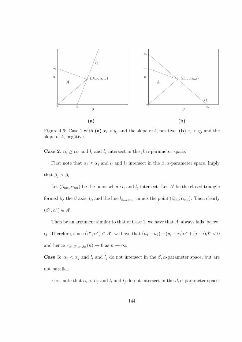
00
β
α
l3αi
β3
(βint, αint)A
00
β
α
l3
αi
α3
β3
(βint, αint)A
(a) (b)
Figure 4.6: Case 1 with (a) xi > yj and the slope of l3 positive. (b) xi < yj and theslope of l3 negative.
Case 2: αi ≥ αj and li and lj intersect in the β, α-parameter space.
First note that αi ≥ αj and li and lj intersect in the β, α-parameter space, imply
that βj > βi.
Let (βint, αint) be the point where li and lj intersect. Let A′ be the closed triangle
formed by the β-axis, li, and the line lβint,αintminus the point (βint, αint). Then clearly
(β∗, α∗) ∈ A′.
Then by an argument similar to that of Case 1, we have that A′ always falls ‘below’
l3. Therefore, since (β∗, α∗) ∈ A′, we have that (h1−h2)+ (yj −xi)α∗+(j− i)β∗ < 0
and hence rα∗,β∗,h1,h2(n) → 0 as n →∞.
Case 3: αi < αj and li and lj do not intersect in the β, α-parameter space, but are
not parallel.
First note that αi < αj and li and lj do not intersect in the β, α-parameter space,
144
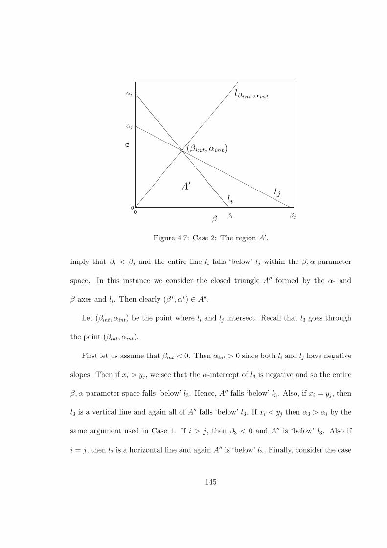
00
β
α
ljli
lβint ,αintαi
βi
αj
βj
(βint, αint)
A′
Figure 4.7: Case 2: The region A′.
imply that βi < βj and the entire line li falls ‘below’ lj within the β, α-parameter
space. In this instance we consider the closed triangle A′′ formed by the α- and
β-axes and li. Then clearly (β∗, α∗) ∈ A′′.
Let (βint, αint) be the point where li and lj intersect. Recall that l3 goes through
the point (βint, αint).
First let us assume that βint < 0. Then αint > 0 since both li and lj have negative
slopes. Then if xi > yj, we see that the α-intercept of l3 is negative and so the entire
β, α-parameter space falls ‘below’ l3. Hence, A′′ falls ‘below’ l3. Also, if xi = yj, then
l3 is a vertical line and again all of A′′ falls ‘below’ l3. If xi < yj then α3 > αi by the
same argument used in Case 1. If i > j, then β3 < 0 and A′′ is ‘below’ l3. Also if
i = j, then l3 is a horizontal line and again A′′ is ‘below’ l3. Finally, consider the case
145

00
β
α
ljli
αi
βi
αj
βj
A′′
Figure 4.8: Case 3: The region A′′.
when xi < yj and i ≤ j. Now, βj > βi, i.e.,
h2
j>
h1
i
and we have that
h2 i > h1 j
h2 i− h1 i > h1 j − h1 i
i (h2 − h1) > h1 (j − i)
146

0
0
β
α
lil3
βi
α3
αi
(βint, αint)
A′′
0
0
β
α
lil3βi
αi
(βint, αint)
A′′
β3
(a) (b)
0
0
β
α
lil3βi
α3
β3
αi
(βint, αint)
A′′
0
0
β
α
li
l3
βi
α3
αi
(βint, αint)
A′′
(c) (d)
0
0
β
α
li l3
αi
βi β3
α3
(βint, αint)
A′′
(e)
Figure 4.9: Case 3 with βint < 0 and (a) xi > yj. (b) xi = yj. (c) xi < yj and i < j.(d) xi < yj and i = j. (e) xi < yj and i > j.
147
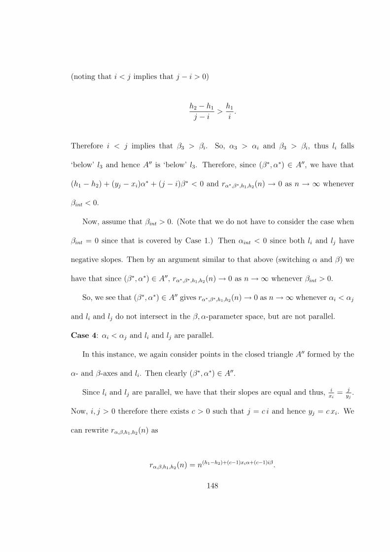
(noting that i < j implies that j − i > 0)
h2 − h1
j − i>
h1
i.
Therefore i < j implies that β3 > βi. So, α3 > αi and β3 > βi, thus li falls
‘below’ l3 and hence A′′ is ‘below’ l3. Therefore, since (β∗, α∗) ∈ A′′, we have that
(h1 − h2) + (yj − xi)α∗ + (j − i)β∗ < 0 and rα∗,β∗,h1,h2(n) → 0 as n → ∞ whenever
βint < 0.
Now, assume that βint > 0. (Note that we do not have to consider the case when
βint = 0 since that is covered by Case 1.) Then αint < 0 since both li and lj have
negative slopes. Then by an argument similar to that above (switching α and β) we
have that since (β∗, α∗) ∈ A′′, rα∗,β∗,h1,h2(n) → 0 as n →∞ whenever βint > 0.
So, we see that (β∗, α∗) ∈ A′′ gives rα∗,β∗,h1,h2(n) → 0 as n →∞ whenever αi < αj
and li and lj do not intersect in the β, α-parameter space, but are not parallel.
Case 4: αi < αj and li and lj are parallel.
In this instance, we again consider points in the closed triangle A′′ formed by the
α- and β-axes and li. Then clearly (β∗, α∗) ∈ A′′.
Since li and lj are parallel, we have that their slopes are equal and thus, ixi
= jyj
.
Now, i, j > 0 therefore there exists c > 0 such that j = c i and hence yj = c xi. We
can rewrite rα,β,h1,h2(n) as
rα,β,h1,h2(n) = n(h1−h2)+(c−1)xiα+(c−1)iβ.
148
00
β
α
ljli
αi
βi
αj
βj
A′′
Figure 4.10: Case 4: The region A′′.
Also, l3 has slope s3 = −(c−1)i(c−1)xi
= −ixi
and is parallel to li and lj.
If c ≤ 1, then (c − 1) ≤ 0 and this along with h1 < h2 implies that (h1 − h2) +
(c − 1)xiα + (c − 1)iβ < 0. Hence rα,β,h1,h2(n) → 0 as n → ∞ for all α, β ≥ 0. If
c > 1 then we see that yj > xi. As in Case 1, yj > xi and αi < αj together imply
that α3 > αi. However, l3 is parallel to li and has a greater α-intercept. Therefore,
li, and hence A′′, falls in the open half space ‘below’ l3. Hence, rα∗,β∗,h1,h2(n) → 0 as
n →∞ since (β∗, α∗) ∈ A′′.
So, (β∗, α∗) ∈ A′′ gives rα∗,β∗,h1,h2(n) → 0 as n →∞ whenever αi < αj and li and
lj are parallel.
Therefore whenever li is under lj at (β, α), we have that rα,β,h1,h2(n) → 0 as
n →∞.
149

QED.
We now generalize this notion of a line being under implying convergence to zero
to ratios of the form ainh1−xiα−β i
gα,β,hg (n). It is indeed true that ain
h1−xiα−β i
gα,β,hg (n)→ 0 as n → ∞,
whenever li is completely under the convex set C(g) in the obvious sense.
Lemma 4.3.4. Let h1, hg,m ∈ Z+ with h1 < hg. Let i, j ∈ {0, 1, . . . , m − 1},
0 < xi, yj ≤ m− 1, and ai = 1 and bj ∈ {0, 1} not all zero. Let
rα,β,h1,g(n) =ain
h1−xiα−β i
gα,β,hg(n)=
ainh1−xiα−β i
∑m−1j=0 bjnhg−yjα−βj
.
Let li be the line h1−xiα−βi = 0 and C(g) be the convex region in which gα,β,hg(n) → 0
as described in Proposition 4.1.1. Then rα,β,h1,g(n) → 0 whenever gα,β,hg(n) →∞ (as
n →∞) and li falls ‘below’ C(g).
Proof :
Let li fall ‘below’ C(g). Let (β, α) be a point in the β, α-parameter space for which
gα,β,hg(n) →∞ as n →∞. Then, (β, α) also falls in the region ‘below’ C(g).
If (β, α) is ‘above’ the line li, then ainh1−xiα−β i → 0 as n → ∞, and clearly,
rα,β,h1,g(n) → 0. Also, if (β, α) is on li, then h1−xiα−β i = 0 and again rα,β,h1,g(n) →
0 as n →∞. So, from now on, we assume that (β, α) is in the region ‘below’ li.
Now, (β, α) is ‘below’ li which is ‘below’ C(g), therefore the line lβ,α will intersect
li ‘below’ C(g). Let (βint, αint) be the point where lβ,α intersects G(β), the boundary
of C(g). Recall that G(β) is a piecewise linear function, whose pieces come from
150
the lines associated with the terms in gα,β,hg(n). Therefore, there must exist some
0 ≤ j ≤ m− 1 for which bj = 1 and (βint, αint) is on the line lj. Therefore, li is under
lj at the point (β, α). Hence, by Lemma 4.3.3, we have that
ainh1−xiα−β i
bjnhg−yjα−β j→ 0
as n →∞. Therefore by Lemma 4.3.1 we have that all of
rα,β,h1,g(n) =ain
h1−xiα−β i
gα,β,hg(n)=
ainh1−xiα−β i
∑m−1j=0 bjnhg−yjα−βj
→ 0
as n →∞.
QED.
So, we have that whenever line li falls in the open region ‘below’ C(g) we have
that the associated term over gα,β,hg(n) goes to 0.
We are now ready for the main theorem of this section.
Theorem 4.3.5. Let fα,β,hf(n), gα,β,hg(n) ∈ F . Let hf < hg and
R(fα,β,hf(n), gα,β,hg(n)) =
fα,β,hf(n)
gα,β,hg(n)=
∑m−1i=0 ain
hf−xiα−βi
∑m−1j=0 bjnhg−xjα−βj
.
Then R(fα,β,hf(n), gα,β,hg(n)) → 0 whenever gα,β,hg(n) → ∞ as n → ∞, if for each
0 ≤ i ≤ m− 1, either ai = 0 or li is ‘below’ C(g).
151
Proof :
First note that R(fα,β,hf(n), gα,β,hg(n)) will only go to zero if and only if for each
0 ≤ i ≤ m− 1, ainh1−xiα−β i
gα,β,hg (n)→ 0.
If ai = 0, then clearly ainh1−xiα−β i
gα,β,hg (n)→ 0. So, let ai = 1 and li be ‘below’ C(g). Then
by Lemma 4.3.4, we have that ainh1−xiα−β i
gα,β,hg (n)→ 0 and hence R(fα,β,hf
(n), gα,β,hg(n)) → 0
as n →∞.
QED.
So, to show that R(fα,β,hf(n), gα,β,hg(n)) goes to zero, it is sufficient to show that
each of the lines associated with fα,β,hf(n) falls ‘below’ the convex set C(g). This
result gives us the following obvious corollary relating the two convex sets C(f) and
C(g).
Corollary 4.3.6. Let fα,β,hf(n), gα,β,hg(n) ∈ F . Let hf < hg and
R(fα,β,hf(n), gα,β,hg(n)) =
fα,β,hf(n)
gα,β,hg(n)
Then R(fα,β,hf(n), gα,β,hg(n)) → 0 whenever gα,β,hg(n) →∞ as n →∞, if F (β) falls
in the region ‘below’ C(g), i.e., if the region C(f) contains the region C(g).
152

Chapter 5
The Discrete Model
In this chapter we present the Discrete Random Dot Product Graph. We begin
by introducing the model and proving basic results in Section 5.1.1. In Section 5.1.2
we illustrate the difficulty of calculations in this model by finding the threshold for
the appearance of K3 as a subgraph. In Section 5.2, we define the probability order
polynomial, or POP, of a graph H, give a general method for calculating the POP
of H, and present formulas for the POPs of trees, cycles, and complete graphs. In
Section 5.3, we present first moment results for trees, cycles, and complete graphs.
We also prove a threshold result for K3 and describe a general method for proving
threshold results when all the required POPs are known.
153

5.1 The 0, 1 Discrete Random Dot Product Graph
In this chapter we study the behavior of the Random Dot Product Graph when
the vectors are drawn from the discrete sample space {0, 1}t, where t ∈ Z≥1. In this
case, each vertex v ∈ V (G) is given a vector xv drawn from {0, 1}t as follows: each
coordinate of xv is independently assigned the value 1 with probability p and the
value 0 with probability 1 − p, where p ∈ [0, 1]. We define the probability mapping
f : R→ [0, 1] to be f(r) = r/t, guaranteeing that the dot product of any two vectors
is mapped into probabilities. We denote this sample space of discrete random dot
product graphs as D[n, {0, 1}t, p].
In [20], Singer introduces Random Intersections Graphs, a random graph model
in which vertices are mapped to random sets in the following way: each vertex v is
assigned a subset Sv of a universal set of t elements, [t], by independently placing
each i ∈ [t] in Sv with probability p. If we view the vector xv as an indicator function
in which element i is placed in Sv if and only if the ith coordinate of xv is one,
then the assignment of vectors to vertices in a Discrete Random Dot Product Graph
is similar to Singer’s assignment of sets to vertices. However, unlike in a Discrete
Random Dot Product Graph, in a Random Intersection Graph, once the sets have
been assigned, the existence of edges is not random, but deterministic, with an edge
between vertices u and v if and only if Su∩Sv 6= ∅. Although the Random Intersection
Graph is different from the discrete model we present in this Chapter, it is a Random
Dot Product Graph model in which the probability mapping f(y) is 0 when y = 0
154
and 1 otherwise.
5.1.1 Basic Results
Proposition 5.1.1. Let G be drawn from D[n, {0, 1}t, p]. For any u, v ∈ V (G) we
have P [u ∼ v] = p2.
Proof:
Let u, v ∈ V (G). Let x = [x1, x2, . . . , xt]T and y = [y1, y2, . . . , yt]
T be the vectors
of u and v respectively. Then
P [u ∼ v] = E[x · y
t] = E[
(x1y1 + · · ·+ xtyt)
t] =
tE[x1y1]
t= E[x1]E[y1] = p2.
QED.
Thus, the probability of an edge is p2 and the expected number of edges is(
n2
)p2.
While, this constant probability on the edges is also common to Erdos-Renyi random
graphs, our graphs are not simply Erdos-Renyi (n, p2). For example in an Erdos-
Renyi (n, p2) random graph the probability that two vertices are adjacent given that
share a common neighbor is again p2. However in this model, the knowledge of the
common neighbor increases the probability of the adjacency, i.e., the model exhibits
clustering.
Lemma 5.1.2. Let G be drawn from D[n, {0, 1}t, p]. For any u, v, w ∈ V (G), we
155

have
P [u ∼ v ∼ w] =1
t2[tp3 + t(t− 1)p4].
Proof:
Let u, v, w ∈ V (G). Let x = [x1, x2, . . . , xt]T , y = [y1, y2, . . . , yt]
T , and z =
[z1, z2, . . . , zt]T , be the vectors of u,v, and w respectively. Then
P [u ∼ v ∼ w] = E[(x · y
t
)(y · zt
)]= E
[(x1y1 + · · ·+ xtyt
t
)(y1z1 + · · ·+ ytzt
t
)]
=1
t2
∑
i,j∈{1,2,...,t}E [xiyiyjzj] .
We now consider what occurs as i and j vary. If i = j, then the term inside
the sum is E[xiyiyjzj] = E[xiy2i zi] = E[xiyizi], since yi ∈ {0, 1}. Furthermore,
E[xiyizi] = E[xi]E[yi]E[zi] = p3, since xi, yi and zi are independent. Also, if i 6= j,
then yi and yj are independent and so the term inside the sum is E[xiyiyjzj] =
E[xi]E[yi]E[yj]E[zj] = p4. Therefore we see that
P [u ∼ v ∼ w] =1
t2
∑
i∈{1,2,...,t}p3 +
∑
i,j∈{1,2,...,t} : i6=j
p4
=
1
t2(tp3 + t(t− 1)p4
).
QED.
Similarly and as will be shown in Section 5.1.2, we obtain the following result.
156

Lemma 5.1.3. Let G be drawn from D[n, {0, 1}t, p]. For any u, v, w ∈ V (G) we have
P [the triangle uvw] =1
t3[tp3 + 3t(t− 1)p5 + t(t− 1)(t− 2)p6].
These two lemmas give us the following result.
Proposition 5.1.4. Let G be drawn from D[n, {0, 1}t, p]. For any u, v, w ∈ V (G) we
have P [u ∼ w|u ∼ v ∼ w] ≥ P [u ∼ w], with equality holding iff p = 1.
Proof:
P [u ∼ w|u ∼ v ∼ w] =P [the triangle uvw]
P [u ∼ v ∼ w]
which from Lemmas 5.1.3 and 5.1.2
=1t3
[tp3 + 3t(t− 1)p5 + t(t− 1)(t− 2)p6]1t2
[tp3 + t(t− 1)p4]
=1 + 3p2(t− 1) + p3(t− 1)(t− 2)
(1 + p(t− 1))t.
So,
P [u ∼ w|u ∼ v ∼ w]− p2 =(1− p)(1 + p + 2p2(t− 1))
1 + p(−1 + t))t≥ 0
since 0 ≤ p ≤ 1 and t ≥ 1 implies that 1 − p ≥ 0, 1 + p + 2p2(t − 1) > 0 and
157
1 + p(t− 1))t > 0. Hence we have that
P [u ∼ w|u ∼ v ∼ w] ≥ p2 = P [u ∼ w]
with equality holding iff p = 1.
QED.
We have already determined that the probability of an edge is p2 and therefore the
expected number of edges is ( n2 )p2. However we would like to know for which values
of p does a Discrete Random Dot Product Graph have edges (with high probability).
Now, to further this discussion we must first calculate the variance on the number of
edges in a Discrete Random Dot Product Graph.
Lemma 5.1.5. Let G be drawn from D[n, {0, 1}t, p]. Let the random variable X be
the number of edges in G. Then
Var[X] =
(n
2
)p2 + 6
(n
3
)p3 + (t− 1)p4
t+
(n
2
)(n− 2
2
)p4 −
(n
2
)2
p4.
Proof:
Consider X as the sum of the indicator functions for each individual edge. So,
X =∑
u,v∈V (G)u<v
I {u ∼ v}. Therefore by Proposition 5.1.1 we have that
E[X] = E
∑
u,v∈V (G)u<v
I{u ∼ v}
=
∑
u,v∈V (G)u<v
E[ I{u ∼ v}] =∑
u,v∈V (G)u<v
P [u ∼ v] =
(n
2
)p2.
158

The variance of X is
Var[X] = E[X2]− E[X]2 = E[X2]−(
n
2
)2
p4
and so we calculate E[X2].
E[X2] = E
∑
u,v∈V (G)
I {u ∼ v}
2
= E
∑
u,v∈V (G)u<v
I2 {u ∼ v} +∑
u,v,w∈V (G)u6=v,u 6=w,v 6=w
I {u ∼ v} I {v ∼ w}
+∑
u,v,w,z∈V (G)u<v,w<z
{u,v}∩{w,z}=∅
I {u ∼ v} I {w ∼ z}
= E
∑
u,v∈V (G)u<v
I2 {u ∼ v}
+ E
∑
u,v,w∈V (G)u6=v,u 6=w,v 6=w
I {u ∼ v} I {v ∼ w}
+E
∑
u,v,w,z∈V (G)u<v,w<z
{u,v}∩{w,z}=∅
I {u ∼ v} I {w ∼ z}
.
We now look at each of the three expected values individually. In the first expected
value, since the indicator random variables can only have the value of 0 or 1 we see
159

that
E
∑
u,v∈V (G)u<v
I2 {u ∼ v}
= E
∑
u,v∈V (G)u<v
I {u ∼ v}
=
∑
u,v∈V (G)u<v
E [ I {u ∼ v}]
=
(n
2
)P [u ∼ v] =
(n
2
)p2.
Next, for the middle term, we have that
E
∑
u,v,w∈V (G)u6=v,u 6=w,v 6=w
I {u ∼ v} I {v ∼ w}
=
∑
u,v,w∈V (G)u6=v,u 6=w,v 6=w
E [I {u ∼ v} I {v ∼ w}]
= 6
(n
3
)E [I {u ∼ v} I {v ∼ w}] .
Now, I {u ∼ v} I {v ∼ w} = 1 if and only if I {u ∼ v} = 1 and I {v ∼ w} = 1, and
is 0 otherwise. Therefore, E [I {u ∼ v} I {v ∼ w}] = P [u ∼ v ∼ w] = p3+(t−1)p4
tby
Lemma 5.1.2. Hence the middle term is
E
∑
u,v,w∈V (G)u6=v,u 6=w,v 6=w
I {u ∼ v} I {v ∼ w}
= 6
(n
3
)p3 + (t− 1)p4
t.
Finally, since the events {u ∼ v} and {w ∼ z} are independent, the last term
160

becomes
E
∑
u,v,w,z∈V (G)u<v,w<z
{u,v}∩{w,z}=∅
I {u ∼ v} I {w ∼ z}
=∑
u,v,w,z∈V (G)u<v,w<z
{u,v}∩{w,z}=∅
E [I {u ∼ v}] E [I {w ∼ z}]
=
(n
2
)(n− 2
2
)P [u ∼ v]P [w ∼ z] =
(n
2
)(n− 2
2
)p4.
Now we have that E[X2] =(
n2
)p2 + 6
(n3
)p3+(t−1)p4
t+
(n2
)(n−2
2
)p4. Therefore the
variance is indeed
Var[X] =
(n
2
)p2 + 6
(n
3
)p3 + (t− 1)p4
t+
(n
2
)(n− 2
2
)p4 −
(n
2
)2
p4.
QED.
Theorem 5.1.6. Let G be drawn from D[n, {0, 1}t, p]. A threshold function for the
appearance of edges in G is p = 1/n. That is, with high probability G will be edgeless
whenever p ¿ 1n
and with high probability G will have at least one edge whenever
p À 1n, irrespective of t.
Proof:
Let the random variable X be the number of edges in G. Then we know from
the proof of Lemma 5.1.5 that E(X) =(
n2
)p2. Let 1/n be our candidate for the
threshold function for the appearance of edges. Now, by Markov’s inequality P [X ≥
1] ≤ E[X] =(
n2
)p2. So whenever the probability p(n) is such that p(n)/(1/n) → 0
161

as n → ∞, we have that E[X] → 0 and therefore the P [X = 0] → 1 as n → ∞ and
almost every graph has no edges.
Also, whenever, p(n)/(1/n) → ∞ as n → ∞, then E[X] → ∞ and we use the
second moment method. By Chebychev’s inequality we know that P [X = 0] ≤
Var(X)/E[X]2. By Lemma 5.1.5 we have that
P [X = 0] ≤ Var[X]
E[X]2=
(n2
)p2 + 6
(n3
)p3+(t−1)p4
t+
(n2
)(n−2
2
)p4 − (
n2
)2p4
((n2
)p2
)2
=
(n2
)p2
((n2
)p2
)2 +6(
n3
)p3+(t−1)p4
t((n2
)p2
)2 +
(n2
)(n−2
2
)p4 − (
n2
)2p4
((n2
)p2
)2 .
Now let us examine the three parts of the sum individually. First,
(n2
)p2
((n2
)p2
)2 =E[X]
E[X]2→ 0
since E[X] →∞ as n →∞. Secondly,
6(
n3
)p3+(t−1)p4
t((n2
)p2
)2 ³ n3p3(1/t) + n3p4
n4p4=
1
np t+
1
n≤ 1
np+
1
n→ 0
since np = p/(1/n) →∞ as n →∞. Finally
(n2
)(n−2
2
)p4 − (
n2
)2p4
((n2
)p2
)2 ≤ 0
.
162

Therefore
P [X = 0] → 0
as n → ∞, for all t ≥ 1. Therefore, whenever p(n)/(1/n) → ∞ almost every graph
will have an edge.
QED.
Hence, 1n
is indeed a threshold function for the appearance of edges in G.
5.1.2 K3 : A Detailed Example
We would like to know the thresholds for the appearance of any given subgraph H
in a Discrete Random Dot Product Graph. However, before we delve into the general
discussion, let us consider the special case when H is K3. First, we recall and prove
Lemma 5.1.3
Lemma 5.1.3 Let G be drawn from D[n, {0, 1}t, p]. For any u, v, w ∈ V (G) we
have
P [the triangle uvw] =1
t3[tp3 + 3t(t− 1)p5 + t(t− 1)(t− 2)p6].
Proof:
Let u, v, w ∈ V (G). Let x = [x1, x2, . . . , xt]T , y = y1, y2, . . . , yt]
T , and z =
[z1, z2, . . . , zt]T , be the vectors of u, v, and w respectively. Then
P [the triangle uvw] = E
[(x · y)
t
(y · z)t
(x · z)t
]
163

= E
[(x1y1 + · · ·+ xtyt)
t
(y1z1 + · · ·+ ytzt)
t
(x1z1 + · · ·+ xtzt)
t
]
=1
t3
∑
i,j,k∈{1,2,...,t}E [xiyiyjzjxkzk]
and we now consider what occurs as i, j, and k vary. If i = j = k, then the term inside
the summation is E[xiyiyjzjxkzk] = E[x2i y
2i z
2i ] = E[xiyizi], since xi, yi, zi ∈ {0, 1}.
Furthermore, E[xiyizi] = E[xi]E[yi]E[zi] = p3 since xi, yi, and zi are indepen-
dent. Also, if i = j 6= k, then the term inside the summation is E[xiyiyjzjxkzk] =
E[xiy2i zixkzk] = E[xiyizixkzk] = E[xi]E[yi]E[zi]E[xk]E[zk] = p5. In a similar manner,
E[xiyiyjzjxkzk] = p5 whenever i = k 6= j and j = k 6= i. Finally, if i, j and k are all
different, then the variables in the expected value are mutually independent and we
have E[xiyiyjzjxkzk] = E[xi]E[yi]E[yj]E[zj]E[xk]E[zk] = p6.
Therefore
P [the triangle uvw] =1
t3
∑
i∈{1,2,...,t}p3 + 3
∑
i,j∈{1,2,...,t}u<v
p5 +∑
i,j,k∈{1,2,...,t}u 6=v,u 6=w,v 6=w
p6
=1
t3[tp3 + 3t(t− 1)p5 + t(t− 1)(t− 2)p6].
QED.
Thus, we can calculate the probability that a specific set of three vertices forms a
K3.
164
For any distinct u, v, w ∈ V (G), let Zu,v,w be the indicator function for the triangle
uvw. Then then total number of K3’s is Z =∑
u,v,w∈V (G)u<v<w
Zu,v,w and we can calculate
the expected number of K3’s
E[Z] = E
∑
u,v,w∈V (G)u<v<w
Zu,v,w
=
∑
u,v,w∈V (G)u<v<w
E[Zu,v,w]
=
(n
3
)1
t3[tp3 + 3t(t− 1)p5 + t(t− 1)(t− 2)p6].
Next, we calculate the variance of Z,
Var[Z] = E[Z2]−E[Z]2 = E[Z2]−(
n
3
)2 (1
t3
)2
[tp3 +3t(t− 1)p5 + t(t− 1)(t− 2)p6]2.
Now let us look more closely at the first term in the variance calculation.
E[Z2] = E
∑
u,v,w∈V (G)u<v<w
Zu,v,w
∑
a,b,c∈V (G)a<b<c
Za,b,c
= E
∑
u,v,w∈V (G)u<v<w
Z2u,v,w + 3
∑
u,v,w,a∈V (G)u<v<w
a6∈{u,v,w}
Zu,v,wZa,v,w
+3∑
u,v,w,a,b∈V (G)u<v<w;a<b
{a,b}∩{u,v,w}=∅
Zu,v,wZa,b,w +∑
u,v,w,a,b,c∈V (G)u<v<w; a<b<c
{a,b,c}∩{u,v,w}=∅
Zu,v,wZa,b,c
165
= E
∑
u,v,w∈V (G)u<v<w
Z2u,v,w
+ 3E
∑
u,v,w,a∈V (G)u<v<w
a 6∈{u,v,w}
Zu,v,wZa,v,w
+3E
∑
u,v,w,a,b∈V (G)u<v<w;a<b
{a,b}∩{u,v,w}=∅
Zu,v,wZa,b,w
+ E
∑
u,v,w,a,b,c∈V (G)u<v<w; a<b<c
{a,b,c}∩{u,v,w}=∅
Zu,v,wZa,b,c
.
So, similarly to the proof of Lemma 5.1.5 we see that
E[Z2] =
(n
3
)P [the triangle uvw]
+
(n
3
)(n− 3)3P [{the triangle uvw} ∩ {the triangle avw}]
+
(n
3
)(n− 3
2
)3P [{the triangle uvw} ∩ {the triangle abw}]
+
(n
3
)(n− 3
3
)P [{the triangle uvw} ∩ {the triangle abc}].
Which, as in the proofs of Lemmas 5.1.2 and 5.1.3, can be calculated exactly and
we have that
Var[Z2] = −(1/(12t5))((−2 + n)(−1 + n)n(−1 + p)p3(2t3 + 2pt(−9 + 3n + t2)
+2p3(−1 + t)t(−62 + 21n + t + t2 + t3) + p2(36 + 3n2 − 18t− 4t3 + 6t4 + 3n(−7 + 2t))
+2p5(−1+t)t(346+6n2−179t+t2+t3+15n(−9+4t))+2p8(−2+t)2(−1+t)(−108+80t−8t2
166
+n2(−9+6t)+3n(21−15t+t2))+2p4(−1+t)(180+15n2−80t−17t2+t3+t4+3n(−35+9t+2t2))
+2p7((2− 3t + t2))(n2(−48 + 33t) + 3n(112− 81t + 3t2 + t3)− 4(144− 107t + 6t2 + 2t3))
+p6(−1+t)(51n2(−3+2t)+3n(357−212t−36t2+16t3)+2(−918+494t+161t2−71t3+t4)))).
We would like to use this variance calculation to determine a threshold function for
the appearance of triangles. However, we must first set some conditions on p and t.
Let us assume that p and t have the forms
• p = 1nα
• t = nβ
where α, β ≥ 0. Then we propose a threshold function for the appearance of triangles
in terms of α and β.
Proposition 5.1.7. Let G be drawn from D[n, {0, 1}t, p]. Let us assume that p and
t have the forms p = 1nα and t = nβ. A threshold for the appearance of triangles in G
is 1/nα where
α(β) =
3−2β3
β ≤ 34
12
β ≥ 34
.
That is, with high probability G will be triangle-free whenever p ¿ 1nα and with high
probability G will have at least one triangle whenever p À 1nα , where α is dependent
167

on β and hence on t.
Proposition 5.1.7 can be proved directly using the previous discussion, however
the task is algebraically tedious and so instead we will show that Proposition 5.1.7 is
a consequence of Theorem 5.3.5.
5.2 The Probability Order Polynomial
5.2.1 Defining the POP
In the previous sections, we discussed the probabilities of the appearance of an
edge, a triangle and a P3 in a Discrete Random Dot Product Graph. More generally,
we would like to study the appearance of any subgraph.
Let’s say that we have a graph H with m edges E(H) = {e1, e2, . . . , em}. Let
us assume that each edge ei ∈ E(H) has endpoints u(ei) and v(ei), so that V (H) =
{u(e1), v(e1), u(e2), v(e2), . . . , u(em), v(em)}. We wish to know the probability of H
appearing as a subgraph of the random graph G (although not necessarily induced).
To this end, we define, P≥[H] = P [H is a subgraph of G] in a specific order 1 when G
is drawn from D[n, {0, 1}t, p]. Then we know by definition that the probability that
H appears on a specific set of vertices is
P≥[H] = E
[(x(e1) · y(e1)
t
)(x(e2) · y(e2)
t
)...
(x(em) · y(em)
t
)]
1Here we mean that H appears a specific set of vertices of G with the specific edges E(H).
168
where x(ei) and y(ei) are the vectors of the endpoints of edge ei, u(ei) and v(ei)
respectively. So, we see that
P≥[H] = E
[(x(e1)1y(e1)1 + · · ·+ x(e1)ty(e1)t
t
)· · ·
· · ·(
x(em)1y(em)1 + · · ·+ x(em)ty(em)t
t
)]
=1
tm
∑
i1,i2,...,im∈{1,2,...t}E[xi1(e1)yi1(e1) xi2(e2)yi2(e2) · · ·xim(em)yim(em)]
and we can calculate the probability by calculating the expected values of the product
xi1(e1)yi1(e1) xi2(e2)yi2(e2) · · · xim(em)yim(em)
for all possible values of the indices i1, . . . , im. However, as seen in Lemmas 5.1.3 and
5.1.2, this can be a complicated task for even small graphs. Also, often we do not
need to know the exact probabilities, but instead are concerned with the behavior in
the limit as n →∞. So, we need to simplify the calculation of P≥[H] while retaining
the basic asymptotic information. To this end, we introduce the following definitions:
Definition 5.2.1. Let f(x, y) and g(x, y) be real valued functions on R2. Then we
say that
f(x, y) ³ g(x, y)
if ∃c1 > 0,∃c2 > 0, so that for all x, y sufficiently small with f(x, y) 6= 0, g(x, y) 6= 0,
169

we have that 0 < c1 ≤ f(x,y)g(x,y)
≤ c2 < ∞.
Proposition 5.2.2. Let ³ be defined on real valued functions on R2 as in Definition
5.2.1. Then ³ is an equivalence relation. Additionally, if we have functions f1, f2, g1,
and g2, positive valued functions, such that f1 ³ g1 and f2 ³ g2 then f1 +f2 ³ g1 +g2.
Proof:
First we show that ³ is an equivalence relation. For any real valued function, f
on R2, 0 < 1 = ff
whenever f 6= 0, and so ³ is reflexive. Let f1, f2 be real valued
function on R2 with f1 ³ f2 then there exist c1, c2 such that 0 < c1 ≤ f1
f2≤ c2 < ∞.
Let a1 = 1c1
and a2 = 1c2
, then 0 < a1, a2 < ∞ and 0 < a2 ≤ f2
f1≤ a1 and hence ³ is
symmetric.
Finally, let f1, f2 and f3 be real valued function on R2 with f1 ³ f2 and f2 ³ f3.
Then there exist c1, c2, d1, d2 such that 0 < c1 ≤ f1
f2≤ c2 < ∞ and 0 < d1 ≤ f2
f3≤
d2 < ∞. Then
0 < c1d1 ≤ f1
f2
f2
f3
=f1
f3
≤ c2d2 < ∞
and ³ is transitive. Therefore, ³ is an equivalence relation on the set of real valued
functions on R2.
Now, let f1, f2, g1, and g2 be positive valued functions such that f1 ³ g1 and
f2 ³ g2. Then there exist c1, c2, d1, d2 such that 0 < c1 ≤ f1
g2≤ c2 < ∞ and
170

0 < d1 ≤ f2
g2≤ d2 < ∞. First note that
g1 + g2
f1 + f2
=g1
f1 + f2
+g2
f1 + f2
<g1
f1
+g2
f2
≤ 1
c1
+1
d1
=c1 + d1
c1d1
.
Therefore taking reciprocals we have that
f1 + f2
g1 + g2
≥ c1d1
c1 + d1
> 0.
Also
f1 + f2
g1 + g2
=f1
g1 + g2
+f2
g1 + g2
<f1
g1
+f2
g2
≤ c2 + d2 < ∞.
Therefore 0 < c1d1
c1+d1≤ f1+f2
g1+g2≤ c2 + d2 < ∞ and f1 + f2 ³ g1 + g2.
QED.
Definition 5.2.3. Let H be a fixed graph with h vertices and m edges. Then the
Probability Order Polynomial of H, gH(p, 1/t), is a polynomial in p and 1/t of the
form
gH(p, 1/t) = px0 +px1
t+
px2
t2+ · · ·+ pxm−2
tm−2+
pxm−1
tm−1
(where x0, x1, . . . , xm−1 ∈ Z≥0) and such that gH(p, 1/t) ³ P≥[H].
One should note that the POP is not the only polynomial that is ³ to P≥[H],
however it is the only one of the form above with all the coefficients equal to one.
Let us consider for a moment how the POP of a graph H relates to the true
probability of the graph appearing, P≥[H]. Recall that
171

P≥[H] =1
tm
∑
i1,i2,...,im∈{1,2,...,t}E[xi1(e1)yi1(e1) xi2(e2)yi2(e2) · · · xim(em)yim(em)]. (5.1)
Now, consider the expectation E[xi1(e1)yi1(e1) xi2(e2)yi2(e2) · · · xim(em)yim(em)].
First note that for all 1 ≤ r ≤ m the random variables xir(er) and yir(er) are inde-
pendent since they are values from vectors that correspond to different vertices. Also,
whenever any two of these random variables have different indices (il 6= ir) then they
are again independent since the random variables are the lth and rth coordinate of
the corresponding vectors and therefore even if they correspond to the same vertex,
they are still different independent random variables. In fact, the only time that
two random variables within the expectation are dependent is when they refer to the
same vertex and vector coordinate, for example when xil(el) = yir(er). Whenever
this occurs we can simplify the product inside the expectation by replacing yir(er) by
xil(el) and then noting that xil(el)xil(el) = xil(el)2 = xil(el) since xil(el) ∈ {0, 1}.
Let us define the following notation for each term of equation (5.1) :
• −→i = (i1, i2, . . . , im) ∈ {1, 2, . . . , t}m is the vector of the set of indices.
• L(−→i ) = [xi1 , yi1 , xi2 , yi2 , . . . , xim , yim ] is the list of vector coordinates.
• X(−→i ) is the number of distinct elements in L(
−→i ).
• V C(−→i ) is the set of elements of L(
−→i ), so X(
−→i ) = |V C(
−→i )|.
172

Then, E[xi1(e1)yi1(e1) xi2(e2)yi2(e2) · · · xim(em)yim(em)] = pX(−→i ) in each term of
Equation (5.1).
Now let S = {i1, i2, . . . , im} the set of values of the indices in a term of Equation
(5.1). Since the summation is over all possible i1, i2, . . . , im ∈ {1, 2, . . . , t}, the size of
the set S will vary from 1 to m depending on how many distinct values are assigned
to the indices. So, the probability of the graph H appearing as a subgraph of G is
P≥[H] =1
tm
m∑
k=1
∑
i1,i2,...,im∈{1,2,...,t}|S|=|{i1,i2,...,im}|=k
E[xi1(e1)yi1(e1) xi2(e2)yi2(e2) · · · xim(em)yim(em)]
=1
tm
m∑
k=1
∑−→i ∈{1,2,...,t}m
|S|=|{i1,i2,...,im}|=k
pX(−→i ).
Let 1 ≤ k ≤ m and consider an assignment of indices in which |S| = k, say S =
{ii, i2, . . . , im} = {j1, j2, . . . , jk} ⊂ {1, 2, . . . , t}, where j1, j2, . . . , jk are distinct . This
assignment corresponds to a partition of the set of edges into k parts, E1, E2, . . . , Ek,
where edge el is in part Er whenever index il is given the value jr. Please note that for
a specific partition E1, E2, . . . , Ek the choice of indices,−→i , that induce this partition
is not unique. In fact, there are (t)k different assignments of the indices that induce
a specific partition of the edge set. To see this, consider a specific k-partition of
the edge set, E1, E2, . . . , Ek and for all 1 ≤ r ≤ k let Sr = {ia : ea ∈ Er}. Then
S =⋃k
r=1 Sr and these sets S1, S2, . . . , Sk define the partition. So, we do not need to
know the exact values j1, j2, . . . , jk associated with S1, S2, . . . , Sk in order to describe
173
the partition. In fact, any of the(
tk
)assignments of the indices induce the same
partition.
Proposition 5.2.4. In the context of the above discussion consider some choice of
the indices i1, i2, . . . , im ∈ {1, 2, . . . , t} for which |S| = k. Let P(−→i ) be the partition
of the edge set of H that corresponds to this set of index values. So, P has k parts,
say E1, E2, . . . , Ek, and for any two edges ea and eb, ea and eb are in the same part if
and only if ia = ib. For all 1 ≤ r ≤ k, let Hr be the graph that is edge induced by part
Er. Let HP(−→i )
= H1⊕H2⊕· · ·⊕Hk be the disjoint union of the edge induced graphs.
Then the number of distinct elements of L(−→i ) is equal to the number of vertices in
HP(−→i )
, i.e.,
X(−→i ) = |V (HP(
−→i )
)|.
Proof:
First note that
|V (HP(−→i )
)| = |V (H1 ⊕H2 ⊕ · · · ⊕Hk)| =k∑
r=1
|V (Hr)|.
Also, recall that V C(−→i ) is the set of vector coordinates in a term of equation (5.1).
So X(−→i ), the number of distinct elements in L(
−→i ), is equal to |V C(
−→i )|. Now, for
each 1 ≤ r ≤ k let V C(−→i , jr) be the set of vector coordinates in a term of equation
(5.1) that correspond to the index jr, i.e., xia , yia ∈ V C(−→i , jr) if and only if ia = jr.
174
Then we have that V C(−→i ) =
⋃kr=1 V C(
−→i , jr) and so
X(−→i ) = |V C(
−→i )| = |
k⋃r=1
V C(−→i , jr)| =
k∑r=1
|V C(−→i , jr)|.
If we can show that |V (Hr)| = |V C(−→i , jr)| for all 1 ≤ r ≤ k then |V (HP(
−→i )
)| =
X(−→i ) and we will be done. We show this by showing that the sets themselves are
equal, i.e. V (Hr) = V C(−→i , jr).
Suppose v ∈ V (Hr). This means that v is an endpoint of at least one edge, say
ea, in Er. So, v = xia or v = yia . Without loss of generality, assume that v = xia .
Now, v = xia ∈ V (Hr) implies that ia = jr. Therefore v = xia ∈ V C(−→i , jr) and so
V (Hr) ⊆ V C(−→i , jr).
Similarly, suppose v ∈ V C(−→i , jr). Then there exists at least one a ∈ {1, 2, . . . ,m}
with xia , yia ∈ V C(−→i , jr), for which v = xia or v = yia . Without loss of generality,
assume that v = xia . Then v is an endpoint of the edge ea. Also, since v = xia ∈
V C(−→i , jr), we have that ia = jr and the edge ea ∈ Er. Therefore the edge ea is in the
set that induces Hr and so the endpoints of ea are in V (Hr). Hence, v = xia ∈ V (Hr)
and so V C(−→i , jr) ⊆ V (Hr).
Therefore we have that V (Hr) = V C(−→i , jr) and so
X(−→i ) =
k∑r=1
|V C(−→i , jr)| =
k∑j=1
|V (Hr)| = |V (HP(−→i )
)|.
QED.
175

So, if we think of the probability in terms of these graphs induced by edge parti-
tions we see that
P≥[H] =1
tm
m∑
k=1
∑−→i ∈{1,2,...,t}m
|S|=|{i1,i2,...,im}|=k
p|V (HP(
−→i )
)|.
Recalling that each partition of the edge set into k parts can occur with(
tk
)different
choices of the index set we have that
P≥[H] =1
tm
m∑
k=1
∑
P(−→i )∈{edge partitions of size k}
(t
k
)p|V (HP(
−→i )
)|
³m∑
k=1
∑
P(−→i )∈{edge partitions of size k}
1
tm−kp|V (HP(
−→i )
)|.
One should note that for each k there are S(m, k) partitions P(−→i ) of size k, where
S(m, k) is the Stirling number of the second kind.
Now since p ∈ [0, 1] for each k we see that
∑
P(−→i )∈{edge partitions of size k}
1
tm−kp|V (HP(
−→i )
)| ³ 1
tm−kphk
where
hk = min−→i : X(
−→i )=k
|V (HP(−→i )
)| =k∑
j=1
|V (Hj)|
is the minimum number of vertices used in a graph induced by an edge partition of
176

size k. Therefore
P≥[H] ³m∑
k=1
1
tm−kphk .
The above discussion gives us the following lemma.
Lemma 5.2.5. Let H be a graph with |E(H)| = m. Let
gH(p, 1/t) = px0 +px1
t+
px2
t2+ · · ·+ pxm−2
tm−2+
pxm−1
tm−1
be the POP of H. Then for all 0 ≤ j ≤ m− 1, xj = hm−j, the minimum number of
vertices used in a graph induced by a partition of the edge set into of m− j parts.
One should note that for any graph H, Lemma 5.2.5 gives us that x0 ≥ x1 ≥
· · · ≥ xm−1.
5.2.2 POPs of Trees, Cycles, and Complete Graphs
While gH is simpler to calculate then the true value of P≥[H], it is still often
complicated. So we will fist consider a few classes of graphs and the POPs that they
produce. We will begin with the often simple class of trees, but first we need the
following results.
Proposition 5.2.6. Let H be a graph on n vertices and m edges without isolated
vertices. Let
gH(p, 1/t) = px0 +px1
t+
px2
t2+ · · ·+ pxm−2
tm−2+
pxm−1
tm−1
177

be the POP of H. Then x0 = 2m and xm−1 = h.
Proof:
By Lemma 5.2.5, x0 = hm−0 = hm and is the minimum number of vertices used
in a graph induced by a partition of the edge set into m parts. The only way to
partition E(H) into m parts is to place each edge into its own part. Therefore
each Hj, 1 ≤ j ≤ m, consists of a single edge and x0 = hm = 2m. Likewise,
xm−1 = hm−(m−1) = h1 and the only way to partition E(H) into 1 part is E(H) itself
which induces H. Therefore xm−1 = h0 = h.
QED.
Lemma 5.2.7. Let H be a graph on h vertices with m edges without isolated vertices.
Let H be another graph formed from H by adding a new pendant edge to H. If the
POP of H is
gH(p, 1/t) = px0 +px1
t+
px2
t2+ · · ·+ pxm−2
tm−2+
pxm−1
tm−1.
Then, the POP of H is
gH(p, 1/t) = px0+2 +m−1∑i=1
pmin{xi+2,xi−1+1}
ti+
pxm−1+1
tm.
Proof:
Let H be a graph on the vertex set V (H) (where |V (H)| = h) and having the
178

edge set E(H) = {e1, e2, . . . , em}. Let H have POP
gH(p, 1/t) = px0 +px1
t+
px2
t2+ · · ·+ pxm−2
tm−2+
pxm−1
tm−1.
Let v be some vertex v ∈ V (H) and H be a graph on V (H) = V (H)⋃{v}, v 6∈ V (H),
with edge set E(H) = E(H)⋃{{v, v}}. So H is a new graph formed from H by adding
a pendant edge to the vertex v ∈ V (H). We wish to calculate the POP of H.
Now, H has exactly one more edge than H and so |E(H)| = |E(H)|+ 1 = m + 1.
Therefore by Lemma 5.2.5 we know that the POP of H has the form
gH(p, 1/t) = py0 +py1
t+
py2
t2+ · · ·+ pym−1
tm−1+
pym
tm
where yj = h(m+1)−j and is the smallest number of vertices in a graph induced by a
partition of the edge set of H into (m+1)− j parts. So to calculate gH(p, 1t), we need
to partition the edges of H into partitions of size 1, 2, . . . , m,m+1. This can be done
by first partitioning the edges e1, e2, . . . , em into partitions of size 1, 2, . . . , m and then
either place the edge {v, v} into one of the existing parts or giving {v, v} its own new
part. Note that partitioning the edges e1, e2, . . . , em is the same as partitioning the
edges of H and that by Lemma 5.2.5 we know that each xj in the POP of H is the
smallest number of vertices in a graph induced by a partition of the edge set of H
into m− j parts. Let us calculate y0, y1, . . . , ym.
Step 1: Calculate y0.
179

By Proposition 5.2.6, y0 = 2|E(H)| = 2(m+1) and x0 = 2|E(H)| = 2m, therefore
y0 = x0 + 2.
Step 2: Calculate yj for 1 ≤ j ≤ m − 1, partitioning the edge set of H into
(m + 1)− j parts.
We can obtain all of the partitions of the edge set of H by partitioning the edges
of H into (m + 1)− j − 1 = m− j parts and then either placing the edge {v, v} into
its own part, an existing part containing v, or an existing part that does not contain
v. We will consider each of these cases separately.
First, for any 1 ≤ j ≤ m− 1, let us consider obtaining a partition of the edge set
of H into (m+1)− j parts by partitioning the edges of H into (m+1)− i− j = m− j
parts, H1, H2, . . . , Hm−j, and then placing the edge {v, v} into its own part. Then
any partition that is formed this way induces a graph on∑m−j
r=1 Hr + |{v, v}| = xj +2
vertices. Therefore, yj ≤ xj + 2.
Now, for any 1 ≤ j ≤ m − 1, consider a partition of the edge set of H into
(m + 1)− j parts obtained from a partition of the edges of H into (m + 1)− j parts
by placing {v, v} into an existing part. Note that the number of vertices used in a
graph induced by just the partition of the edges of H into (m + 1)− j = m− (j − 1)
parts is xj−1. Now, if {v, v} is placed into an existing part that does not contain v
then the graph that the partition induces will contain 2 additional vertices and so the
total number of vertices used will be xj−1 + 2 and so yj ≤ xj−1 + 2.
Finally, since v ∈ V (H) and H does not contain isolated vertices, we know that
180

in every partition of the edges of H we can always find a part that contains v. So, if
{v, v} is placed into an existing part that contains v, then the total number of vertices
that is used in a graph induced by the partition only increases by one. Therefore in
the partition that uses the minimum number of vertices we can always place {v, v}
in a part already containing v and we have that yj ≤ xj−1 + 1.
Since all partitions of H can be obtained from partitions of H in the above manner
we see that the smallest number of vertices required in a partitioning of the edge set
of H into (m + 1)− j parts is yj = min{xj + 2, xj−1 + 1}.
Step 3: Calculate ym.
By Proposition 5.2.6, ym = |V (H)| = h + 1 and xm−1 = |V (H)| = h, therefore
ym = xm−1 + 1.
Thus, the POP of H is
gH(p, 1/t) = px0+2 +m−1∑i=1
pmin{xi+2,xi−1+1}
ti+
pxm−1+1
tm.
QED.
Theorem 5.2.8. Let T be a tree on h ≥ 2 vertices then the POP of T is
gT (p,1
t) = p2(h−1) +
p2(h−1)−1
t+ · · ·+ ph+1
th−3+
ph
th−2=
h−2∑i=0
p2(h−1)−i
ti.
Proof:
The proof is by induction on the number of vertices h. Note that by Proposition
181

5.1.1 and Lemma 5.1.2 we see that the theorem holds when h = 2, 3.
Assume that the theorem holds for all trees on h− 1 vertices and let us consider
a tree, T , on h vertices. Now, since T is a tree, it must contain at least two leaves.
Let v be a leaf of T . Then the subgraph H formed by removing the leaf v from T is
a tree on h− 1 vertices. Therefore the POP of H is
gH(p,1
t) = p2[(h−1)−1] +
p2[(h−1)−1]−1
t+ · · ·+ p[(h−1)−1]+2
t[(h−1)−1]−2+
p[(h−1)−1]+1
t[(h−1)−1]−1
by the induction hypothesis. Now, we use Lemma 5.2.7 to find the POP of T from the
POP of H. In the context of Lemma 5.2.7, xi = 2[(h− 1)− 1]− i = 2(h− 1)− (i+2)
and e = h− 2 and so
fT (p, 1/t) = px0+2 +e−1∑i=1
pmin{xi+2,xi−1+1}
ti+
pxe−1+1
te
= p2(h−1)−(0+2)+2 +
(h−2)−1∑i=1
pmin{2(h−1)−(i+2)+2,2(h−1)−((i−1)+2)+1}
ti+
p2(h−1)−((h−2)−1+2)+1
th−2
= p2(h−1) +h−3∑i=1
pmin{2(h−1)−i,2(h−1)−i+1−2+1}
ti+
p(h−1)+1
th−2
= p2(h−1) +h−3∑i=1
pmin{2(h−1)−i,2(h−1)−i}
ti+
ph
th−2
= p2(h−1) +h−3∑i=1
p2(h−1)−i
ti+
ph
th−2
which is the desired result. Therefore, by induction, the theorem holds for all trees
182

on two or more vertices.
QED.
Theorem 5.2.9. Let Ch be a cycle on h ≥ 3 vertices then the POP of Ch is
gCh(p,
1
t) = p2h +
p2h−1
t+ · · ·+ ph+2
th−2+
ph
th−1=
h∑
k=2
ph+k
th−k+
ph
th−1.
For example the POP of C5 is gC5(p,1t) = p10 + p9
t+ p8
t2+ p7
t3+ p5
t4.
Proof:
Recall that by Definition 5.2.3 and Proposition 5.2.6 the POP of Ch has the general
form
gCh(p, 1/t) = p2h +
px1
t+
px2
t2+ · · ·+ pxh−2
th−2+
ph
th−1.
We would like to show that
gCh(p, 1/t) = p2h +
h−1∑
k=2
ph+k
th−k+
ph
th−1.
In other words, we would like to show that for all 2 ≤ k ≤ h− 1, xh−k = h+ k, which
by Lemma 5.2.5 is equivalent to showing that the minimum number of vertices used
in a graph induced by a partition of the edge set into k parts is hk = h + k.
Let us consider when the edges are partitioned into 2 ≤ k ≤ h− 1 parts.
Claim: The partition of the edge set into a single path Ph−(k−2) and (k − 1) K2s
induces a graph that uses the minimum number of vertices hk.
183

The partition of the edge set into a single Ph−(k−2) and (k−1) K2s induces a graph
that uses h− (k− 2) + (k− 1)2 = h− k + 2 + 2k− 2 = h + k vertices, therefore if the
claim is true then hk = h + k and we are done.
Proof of claim by smallest counterexample: First consider when k = 2. We
wish to partition the edge set into 2 parts. If we partition the edge set into a Ph and
a K2 we use h + 2 vertices. We claim that this is best. Note that for any partition of
the edge set into 2 parts, say E1 and E2 the components of each part will be paths.
Therefore, for each i = 1, 2, the number of vertices in a graph Hi induced by Ei will
be |E(Hi)|+(number of components in Hi). Since each part induces a graph with at
least one component, the total number of vertices used in a graph induced by this
partition is at least |E(H1)|+1+ |E(H2)|+1 = |E(Ch)|+2 = h+2. Hence hk = h+2
and the claim is true for the base case k = 2.
Next, let 2 < k ≤ h− 1 be the smallest value for which the claim fails. So, by our
induction assumption, a partition of the edges of Ch into k − 1 parts that induces a
graph with the minimum number of vertices is the partition of Ch into a Ph−((k−1)−2)
path and (k − 2)K2s which uses hk−1 = h− k − 3 + 2(k − 2) = h + k − 1 vertices.
Also, by our assumption the partition of the edges set into a Ph−k−2 and (k−1)K2s
which uses h + k vertices is not the best case. Therefore, there exists a k-partition
of the edges of Cn that induces a graph that uses at most h + k − 1 vertices. Now
consider one of these best k-partitions, say E1, E2, . . . , Ek. We know that each part
of this partition induces a graph whose components are paths. Therefore there must
184

be a leaf u in H1. Now, u has degree two in Ch, therefore u must appear in some
Hi (i 6= 1). Combine E1 and Ei into a single part and create a new partition that
contains this union and the remaining parts Ej, (j 6= 1, i). This new partition induces
a graph that uses at least 1 fewer vertices than the original partition since u appears
only once. Therefore the new partition uses at most h+k−1−1 = h+k−2 vertices,
however it has k − 1 parts. This is a contradiction since we have already determined
that the best k−1 partitioning induces a graph that uses h+k−1 vertices. Therefore
our assumption is false and no such smallest k exists. Hence for all 2 ≤ k ≤ h − 1
the claim holds.
Therefore the POP of Ch is indeed gCh(p, 1/t) = p2h +
∑h−1k=2
ph+k
th−k + ph
th−1 .
QED.
Now let us move onto a harder class of graphs: the set of complete graphs. We
prove the following lemma before we state the main result.
Lemma 5.2.10. Let H be a connected graph and for all 1 ≤ k ≤ |E(H)|, let hk be
the minimum number of vertices used in a graph induced by a partition of the edge
set of H into k parts. Then hk−1 < hk.
Proof:
Let H be a connected graph. Let Pk be a partition of the edges of H into k parts
that induces a graph with hk vertices. Since H is connected, there exists parts Ei and
Ej that induce graphs Hi and Hj for which V (Hi)⋂
V (Hj) 6= ∅. Therefore, there
exists v ∈ V (Hi)⋂
V (Hj). We can obtain a partition of the edges of H into k − 1
185
parts by taking the union Ei
⋃Ej as a single part and combining it with the other
k − 2 parts from our original k-partition. This new partition will induce a graph
with at least one fewer vertex since v now appears only once in Ei
⋃Ej. Therefore
hk−1 ≤ hk − 1.
QED.
Theorem 5.2.11. Let Kh be the complete graph on h ≥ 4 vertices and let 1 ≤ k ≤(
h2
). Then a partition of the edge set, E(Kh), into k parts that induces a graph with
the minimum number of vertices is found by partitioning E(Kh) into k−1 single edge
sets, E1, E2, . . . , Ek−1, and one large set, Ek, of size(
h2
)− (k−1) that induces a graph
Hk that contains a clique of size ck (where ck maximizes(
ck
2
) ≤ (h2
)− (k− 1)) and at
most one other vertex incident to(
h2
)− (k− 1)− (ck
2
)edges. Therefore, |V (Hk)| = bk
where(
bk−12
)<
(h2
)− (k − 1) ≤ (bk
2
)and the POP of Kh is
gKh(p, 1/t) =
(h2)∑
k=1
p bk+2(k−1)
t(h2)−k
.
Proof:
By Definition 5.2.3 of the POP and Lemma 5.2.5, we know that gKh(p, 1/t) has
the form
gKh(p, 1/t) =
(h2)−1∑i=0
pxi
ti
where xi = h(h2)−i is the minimum number of vertices used in a graph induced by a
186
partition of the edges set into(
h2
)− i parts. We would like to show that
gKh(p, 1/t) =
(h2)−1∑i=0
ph(h2)−i
ti=
(h2)∑
k=1
p bk+2(k−1)
t(h2)−k
. (5.2)
In the second summation of Equation 5.2 we have reversed the order of the terms.
We can reorder the first summation by using the change of index k =(
h2
)− i. Then
gKh(p, 1/t) =
(h2)∑
k=1
px(h2)−k
t(h2)−k
=
(h2)∑
k=1
p bk+2(k−1)
t(h2)−k
.
Showing that Equation 5.2 holds is equivalent to showing that for all 1 ≤ k ≤ (h2
),
bk + 2(k − 1) = x(h2)−k = hk and is the minimum number of vertices used in a graph
induced by a partition of the edge set into k parts.
The partition as described in the statement of the theorem induces a graph that
uses bk + 2(k − 1) vertices, since |V (H1)| = |V (H2)| = · · · = |V (Hk−1)| = 2 and
|V (Hk)| = bk. So, if we can show that this partition does indeed minimize the
number of vertices used in an induced graph, then hk = bk +2(k−1) and the theorem
holds. The rest of the proof is devoted to showing this fact.
First note that such a partition exists and is easily obtained from Kh by systemat-
ically removing edges incident with v1 until no more remain and then repeating with
the edges incident to v2 and so forth, until k − 1 edges have been removed.
We will now prove this theorem by the smallest counter example technique. Let
us first consider the base cases when k = 1, 2.
187

When k = 1, we partition the edge set into a single part E1 = E(Kh). Therefore
the graph induced by this partition is Kh and has h vertices. Hence, the minimum
number of vertices used in a partition of the edge set into 1 part is h1 = h. Also,
b1 is such that(
b1−12
)<
(h2
) − (1 − 1) =(
h2
) ≤ (b12
). Therefore, b1 = h and so
bk + 2(k − 1) = b1 + 2(1− 1) = b1 = h = h1 and the theorem holds when k = 1.
Let k = 2. Then we need(
b2−12
)<
(h2
) − (2 − 1) ≤ (b22
), therefore recalling that
h ≥ 4, it follows that b2 = h and we want to show that h2 = h + 2. Let us assume
otherwise, that is let us assume that there exists a partition of the edge set into 2 parts
that uses at most h+1 vertices. Each part must induce a graph that contains at least
3 vertices, otherwise the partition would be of the type described in the statement of
the theorem and would use h+2 vertices. Let parts E1 and E2 induce graphs H1 and
H2, respectively. Also, let ri = |V (Hi)|, i = 1, 2, then r1 + r2 ≤ h + 1 and r1, r2 ≥ 3.
Now, consider a vertex u ∈ V (Kh), u must by in one or both of H1 and H2. Let
us first consider the case when u is in only one of the induced graphs. Without loss
of generality assume that u ∈ H1 and u 6∈ H2. Now, since the graph is complete, u
is adjacent to all of the other h − 1 vertices in V (Kh) − {u} = {v1, v2, . . . vk−1} in
Kh. Therefore the edges uv1, uv2, . . . , uvk−1 must appear in the partition, and since
u 6∈ H2, these edges must all be in E1. Therefore, v1, v2, . . . , vk−1 ∈ V (H1) and so
r1 = h. Hence r1 + r2 ≥ h + 3 which is a contradiction. Therefore u must appear in
both H1 and H2.
Let us assume that u ∈ V (H1) and u ∈ V (H2). Now, u ∈ V (H2) implies that
188

there is some other vertex v ∈ H2 with u ∼ v and uv ∈ E2. Now, if v is only in V (H2)
and not in V (H1) then by the same argument as above, all of the vertices must be in
V (H2) and so r2 = h, implying again that r1+r2 ≥ h+3 and we have a contradiction.
Therefore v must also appear in both induced graphs. Now all h vertices in Kh must
appear in at least one of the induced graphs and u and v appear in both of them,
therefore r1 + r2 ≥ h + 2 which again is a contradiction.
So, there cannot exist a partition of the edge set that induces a graph with fewer
than h + 2 = b2 + 2 vertices and so our theorem holds when k = 2.
Let us consider the smallest k for which the theorem does not hold (noting that
k ≥ 3). So, there exists a partition E1, E2, . . . , Ek of the edge set into k parts that
induces a graph on hk < bk + 2(k − 1) vertices, however, the theorem holds for all
partitions of size less than k and so hk−1 = bk−1 + 2(k − 2). Now by Lemma 5.2.10,
we have that hk ≥ hk−1 + 1 = bk−1 + 2(k − 2) + 1. Also, by definition of bk it is easy
to see that bk ≤ bk−1 ≤ bk + 1 and so we have that
bk + 2(k − 1) > hk ≥ hk−1 + 1 = bk−1 + 2(k − 2) + 1 ≥ bk + 2(k − 1)− 1.
Therefore hk = hk−1 + 1 and we have the following claims.
Claim 1: |V (Hi)⋂
V (Hj)| ≤ 1 for all i 6= j.
Proof of Claim 1: Suppose that there exists parts Ei and Ej which induce
graphs Hi and Hj for which |V (Hi)⋂
V (Hj)| ≥ 2. Then we can obtain a partition of
189

size k−1 from this partition of size k by taking the union Ei
⋃Ej as a single part and
combining it with the other k− 2 parts from our k-partition. This new partition will
use at most hk − 2 vertices since there are two vertices in the intersection of V (Hi)
and V (Hj) that appeared twice in the k-partition and will only appear once in the
new partition. Therefore hk−1 ≤ hk − 2 = hk−1 + 1 − 2 = hk−1 − 1 and we have a
contradiction. Hence, Claim 1 holds.
Claim 2: Each induced graph Hi a clique.
Proof of Claim 2: Suppose that there exists a part Ei that induces a graph Hi
that is not a clique. Therefore, there exist u, v ∈ V (Hi) for which uv 6∈ Ei. Now, since
the graph is complete, the edge uv must be in some part Ej, i 6= j. So, u, v ∈ V (Hj)
and V (Hi)⋂
V (Hj) ≥ 2 which contradicts Claim 1. Hence, Claim 2 holds.
Now, without loss of generality, let us assume that the the partition is such that
r1 ≥ r2 ≥ · · · ≥ rk. Let us consider H1 and H2. Note that r1 ≥ r2 ≥ 3 otherwise if
2 ≥ r2 ≥ · · · ≥ rk we would have a partition of the type described in the statement of
the theorem and hk = bk + 2(k − 1). Let us assume that V (H1)⋂
V (H2) = ∅. Then
there exists a vertex u ∈ V (H2), with u 6∈ V (H1) and consider the new partition
E1, E2, . . . , Ek formed from E1, E2, . . . , Ek in the following way:
Step 1. Let E2 = E2−{uv : v 6= u, uv ∈ E2}, i.e., E2 is formed from E2 by deleting
all edges incident with u. This step removes u from H2 and V (H2) = V (H2) − {u}.
Note that since r2 ≥ 3 there is at least 2 edges in E2.
Step 2. Let V (H1) = {x1, x2, . . . , xr1} and consider the parts Ei1 , Ei2 , . . . , Eir2−1
190

that contain the edges ux1, ux2, . . . , uxr2−1 respectively. Note that E1, E2 6∈ {Ei1 , Ei2 ,
. . . , Eir2−1} since u 6∈ V (H1) and none of the x′is are in V (H2). Also note that
whenever a 6= b, Eia 6= Eib , otherwise uxa, uxb ∈ Eia and |V (H1)⋂
V (Hia)| = 2
which contradicts Claim 1. We now let E1 = E1
⋃Ei1
⋃ · · ·Eir2−1 so that H1 contains
H1, Hi1 , . . . , Hir2−1 as subgraphs.
Step 3. Place the r2 − 1 edges in {uv : v 6= u, uv ∈ E2} into single edge sets
Ei1 , Ei2 , . . . , Eir2−1 .
Step 4. For all j 6∈ {1, 2, i1, i2, . . . , ir2−1} let Ej = Ej.
This new partition has exactly k parts, E1, E2, . . . , Ek. We want to show that it
also induces a graph on hk vertices.
First note that V (H2) = V (H2) − {u} and so r2 = r2 − 1. Next, ri1 = ri2 =
· · · = rir2−1 = 2 since the graphs are induced by a single edge. Also note that for all
j 6∈ {1, 2, i1, i2, . . . , ir2−1} let rj = rj since the graphs are the same. Finally we have
the following claim:
Claim 3: r1 = r1 + 1 +∑r2−1
l=1 ril − 2(r2 − 1).
Proof of Claim 3: V (H1) = V (H1)⋃{u}⋃r2−1
l=1 V (Hil) by definition. Also
|V (H1)⋃{u}| = r1 + 1 since u 6∈ V (H1). Now for all l, V (H1)
⋂V (Hil) = {xl}
since xl ∈ V (H1) and xl ∈ V (Hil) and by Claim 1 there intersection contains at
most 1 vertex. Also, for all a 6= b, V (Hia)⋂
V (Hib) = {u} since u ∈ V (Hia)
and u ∈ V (Hib) and by Claim 1 there intersection contains at most 1 vertex. So
each vertex in V (H1) = V (H1)⋃{u}⋃r2−1
l=1 V (Hil) appears exactly once in the sets
191

V (H1), {u}, V (Hi1), V (Hi2), . . . , V (Hir2−1) except for u and x1, x2, . . . , xr2−1. Now, u
appears in each of V (Hil) as well as as in {u} and so u appears exactly 1 + r2 − 1
times. Each of the x1, x2, . . . , xr2−1 appear exactly twice, once in V (H1) and once in
their respective V (Hil)’s. Therefore when we sum the sizes of the sets we over count
by r2− 1 for u and r2− 1 for each of the xl’s. Hence r1− r1 +1+∑r2−1
l=1 ril − 2(r2− 1)
and the claim in proven.
So the number of vertices used in a graph induced by the new partition is
k∑j=1
rj =
[r1 + 1 +
r2−1∑
l=1
ril − 2(r2 − 1)
]+ [r2 − 1] + [2(r2 − 1)] +
∑
l 6∈{1,2,i1,i2,...,ir2−1}rl
=k∑
j=1
rj + 1− 2(r2 − 1)− 1 + 2(r2 − 1)
=k∑
j=1
rj
= hk.
Therefore this partition also induces a graph on the minimum number of vertices.
However, H1 is not a clique since only r2 − 1 ≤ r1 − 1 < r1 edges exist between u
and other vertices in V (H1) and there are at least the original r1 other vertices from
V (H1) in V (H1). This fact contradicts Claim 2. Therefore hk cannot be less than
bk + 2(k− 1) and the theorem holds if the intersection of V (H1) and V (H2) is empty.
Let us assume that V (H1)⋂
V (H2) 6= ∅. Therefore by Claim 1 they intersect at
192

exactly one vertex w. Here as above, there exists u ∈ V (H2) with u 6∈ V (H1). We will
create the new k-partition in the same way as above, except that we will put the edge
uw into E1. So, in Step 3, we will only have r2 − 2 single edge sets (note r2 − 2 ≤ 1
since r2 ≤ 3). And in Step 2 we assume that V (H1) = {w, x1, . . . , xh−1} and we add
the edge uw to E1 and only need to add r2 − 2 additional parts Ei1 , Ei2 , . . . , Eir2−1 .
Then Claim 3 becomes:
Claim 3 ′: r1 = r1 + 1 +∑r2−2
l=1 ril − 2(r2 − 2)
The proof of Claim 3 ′ is the similar to that of Claim 3 and the number of vertices
used in a graph induced by the new partition is
k∑j=1
rj =
[r1 + 1 +
r2−2∑
l=1
ril − 2(r2 − 2)
]+ [r2 − 1] + [2(r2 − 2)] +
∑
l 6∈{1,2,i1,i2,...,ir2−2}rl
=k∑
j=1
rj + 1− 2(r2 − 2)− 1 + 2(r2 − 2)
=k∑
j=1
rj
= hk.
Again this new partition induces a graph on the minimum number of vertices.
However, H1 is not a clique since only r2 − 2 + 1 ≤ r1 − 1 < r1 edges exist between
u and other vertices in V (H1) and there are at least the original r1 other vertices
193

from V (H1) in V (H1). This fact contradicts Claim 2. Therefore hk cannot be less
than bk + 2(k − 1) and the theorem holds if the intersection of V (H1) and V (H2)is
nonempty.
Hence there is no smallest k for which there exists a partition that induces a graph
on less than bk + 2(k − 1) vertices. Therefore hk = bk + 2(k − 1) and the Theorem
holds.
QED.
So, for example, the POP of K4 is gK4(p, 1/t) = p12 + p11
t+ p9
t2+ p8
t3+ p6
t4+ p4
t5.
Corollary 5.2.12. Let Kh be the complete graph on h ≥ 2 vertices. Then the POP
if Kh is
gKh(p, 1/t) =
(h2)∑
k=1
p bk+2(k−1)
t(h2)−k
where bk satisfies(
bk−12
)<
(h2
)− (k − 1) ≤ (bk
2
).
Proof:
Let h = 2 so that K2 is a single edge. Then by Proposition 5.1.1 we know that
gK2(p, 1/t) = p2 and we must show that p2 =∑(h
2)k=1
p bk+2(k−1)
t(h2)−k
. First(
h2
)=
(22
)= 1
and so∑(h
2)k=1
p bk+2(k−1)
t(h2)−k
= p b1 . Also, b1 must satisfy(
b1−12
)<
(h2
)− (1− 1) = 1 ≤ (b12
),
and so b1 = 2. Therefore gK2(p, 1/t) =∑(2
2)k=1
p bk+2(k−1)
t(22)−k
= p2.
Let h = 3 so that K3 is a triangle. Then by Lemma 5.1.3 we know that gK3(p, 1/t) =
194

p3
t2+ p5
t+ p6. Now,
(h2
)=
(32
)= 3 and so
(h2)∑
k=1
p bk+2(k−1)
t(h2)−k
=p b1
t2+
p b2+2
t1+ p b3+4.
Now, b1 must satisfy(
b1−12
)<
(32
) − (1 − 1) = 3 ≤ (b12
)and so b1 = 3. Similarly, b2
must satisfy(
b2−12
)<
(32
)− (2− 1) = 2 ≤ (b22
), and so b2 = 3. Finally, b3 must satisfy
(b3−1
2
)<
(32
)− (3− 1) = 1 ≤ (b32
), and so b3 = 2. So,
(h2)∑
k=1
p bk+2(k−1)
t(h2)−k
=p b1
t2+
p b2+2
t1+ p b3+4 =
p 3
t2+
p 5
t1+ p 6
and is the POP of K3.
Also, for all h ≥ 4, we have by Theorem 5.2.11 that gKh(p, 1/t) =
∑(h2)
k=1p bk+2(k−1)
t(h2)−k
is the POP of Kh. Therefore the corollary holds for all h ≥ 2.
QED.
Theorems 5.2.8 and 5.2.9 and Corollary 5.2.12 state the POP of trees, cycles, and
complete graphs. We would like to know the POP of a any graph H. Currently,
if given a specific graph H we can calculate its POP by calculating the minimum
number of vertices used in graphs induced by a partitions of the edge set (Lemma
5.2.5), however we do not yet have a general form for the POP of H.
195

5.3 Towards a Threshold Result
In this section we present first moment results for trees, cycles, and complete
graphs and a threshold result for K3. We are able to prove threshold results for small
specific graphs, but not in general. However, we are able to describe a general method
for proving threshold results if all required POPs are known. The proof of this result,
and others in this section, rely heavily on the framework built in Chapter 4.
5.3.1 The First Moment
In this section, we assume that H is a graph on h > 0 vertices and m > 0 edges.
Also, G is a Discrete Random Dot Product Graph drawn from D[n, {0, 1}t, p]. Finally,
ZH is the number of copies of H in a realization of G.
As first discussed in Section 5.1.2, in any further discussion of the POP, we need
to set some conditions on p and t. So, we assume that p and t have the forms p = 1nα
and t = nβ, where α, β ≥ 0. Then the POP of H will have the form
gH(p, 1/t) = px0 +px1
t+
px2
t2+ · · ·+ pxm−2
tm−2+
pxm−1
tm−1
= (1
nα)x0 +
( 1nα )x1
(nβ)+
( 1nα )x2
(nβ)2+ · · ·+ ( 1
nα )xm−2
(nβ)m−2+
( 1nα )xm−1
(nβ)m−1
=m−1∑i=0
( 1nα )xi
(nβ)i.
Furthermore, the expected number of copies of H in a Discrete Random Dot
196

Product Graph G is
E[ZH ] ³(
n
h
)gH(p, 1/t) ³ nh
m−1∑i=0
( 1nα )xi
(nβ)i=
m−1∑i=0
nh−xiα−βi.
Also, by Lemma 5.2.5 and Proposition 5.2.6 we have that 0 < h ≤ xi ≤ 2m for all
0 ≤ i ≤ m−1. So, E[ZH ] is a posynomial of the form discussed in Chapter 4, with all
of the ai = 1 and all of the ordered pairs, (β, α), points in the β, α-parameter space.
Therefore, if we let fHα,β,h(n) =
∑m−1i=0 nh−xiα−βi, then fH
α,β,h(n) ³ E[ZH ]. Proposition
4.1.1 gives that E[ZH ] → 0 whenever (β, α) ∈ C(fH) and E[ZH ] → ∞ whenever
(β, α) ∈ ζ(fH). So, we see that p = 1nα , where α is the piecewise linear boundary
function α = FH(β), is a candidate for the threshold of the appearance of H in G.
Let us examine this possible threshold function for the classes of graphs for which
we can explicitly calculate the POPs. First, we consider the class of trees on h ≥ 2
vertices.
Proposition 5.3.1. Let G be drawn from D[n, {0, 1}t, p] with p = 1nα and t = nβ for
α, β ≥ 0. Let T be a tree on h ≥ 2 vertices. Let
f′T
α,β,h(n) = nh−2(h−1)α + nh−h α−β (h−2).
Then then the expected number of copies of T in G is
E[ZT ] ≡ f′T
α,β,h(n)
197

with E[ZT ] → 0 whenever (β, α) ∈ C(f′T ) and E[ZT ] →∞ whenever (β, α) ∈ ζ(f
′T ).
Additionally, the boundary function for C(f′T ) is
α =
h−(h−2)βh
β ≤ h2h−2
h2h−2
β ≥ h2h−2
.
Proof:
First recall from Theorem 5.2.8 that the POP of the tree T is
gT (p,1
t) = p2(h−1) +
p2(h−1)−1
t+ · · ·+ ph+1
th−3+
ph
th−2=
h−2∑i=0
p2(h−1)−i
ti.
Therefore the expected number of copies of T in G is
E[ZT ] ³(
n
h
)gT (p, 1/t) ³ fT
α,β,h(n) =h−2∑i=0
nh−(2(h−1)−i)α−βi
= nh−2(h−1)α +
(h−3∑i=1
nh−(2(h−1)−i)α−βi
)+ nh−hα−β(h−2)
= f′T
α,β,h(n) +h−3∑i=1
nh−(2(h−1)−i)α−βi.
If we show that fTα,β,h(n) ≡ f
′Tα,β,h(n) then we will be done.
198

In the context of Chapter 4, for each 0 ≤ i ≤ h− 2 let li be the line
h− (2(h− 1)− i)α− βi = 0.
Then by Proposition 4.1.1, C(fT ) is determined by l0, . . . , lh−2 and C(f′T ) is de-
termined by l0 and lh−2. If we can show that C(fT ) is determined by just l0 and
lh−2, then clearly C(fT ) = C(f′T ) and hence by Proposition 4.2.2 we will have that
fTα,β,h(n) ≡ f
′Tα,β,h(n). Recall that by Proposition 4.2.3, to show that C(fT ) is deter-
mined by just l0 and lh−2, it is sufficient to show that for each i ∈ {1, . . . , h − 3}, li
falls ‘below’ C(f′T ), the convex set determined by l0 and lh−2.
Now, l0 is the horizontal line h − 2(h − 1)α = 0 and has α-intercept α0 = hh−2
.
Also, lh−2 is the line h− hα− β (h− 2) = 0 and has α-intercept αh−2 = 1. Finally, l0
and lh−2 intersect within the β, α-parameter space at the point ( h2h−2
, h2h−2
).
0 10
1
β
α
(h
2h − 2,
h
2h − 2)
· · · · · l0—— lh−2
0 10
1
β
α
(h
2h − 2,
h
2h − 2)
C(f′T )
αi
· · · · · · li
(a) (b)
Figure 5.1: (a) The lines that define C(f′T ). (b) li intersects C(fT ) at exactly one
point.
199

Now, let i ∈ {1, . . . , h− 3} we wish to show that li : h− (2(h− 1)− i)α− βi = 0
falls ‘below’ C(f′T ). The line li has α-intercept αi = h
2h−2−i. Also, i ≤ h−3, implying
that 2h − 2 − i ≥ 2h − 2 − h + 3 = h + 1 > h. Therefore, αi = h2h−2−i
< 1 = αh−2
and the α-intercept of li is below that of lh−2. Next, it is easy to see that li also
goes through point ( h2h−2
, h2h−2
), the intersection point of l0 and lh−2. Finally, li has
negative slope, − i2(h−1)−i
. Hence, li intersects the boundary of C(fT ) at exactly one
point.
So, by Propositions 4.2.3 and 4.2.5 we see that f′T
α,β,h(n) can be obtained from
fTα,β,h(n) by removing each of the terms associated with the lines li, 1 ≤ i ≤ h − 3,
and furthermore f′T
α,β,h(n) = f red Tα,β,h (n). Hence f
′Tα,β,h(n) ≡ fT
α,β,h(n) and so E[ZT ] ≡
f′T
α,β,h(n) with E[ZT ] → 0 whenever (β, α) ∈ C(f′T ) and E[ZT ] → ∞ whenever
(β, α) ∈ ζ(f′T ).
QED.
Therefore, by Markov’s inequality P [ZT ≥ 1] ≤ E[ZT ] → 0 as n →∞, whenever
(β, α) ∈ C(f′T ) and almost no graph contains T . Additionally, p = 1
nα , where α is
the piecewise linear boundary of C(f′T ),
α =
h−(h−2)βh
β ≤ h2h−2
h2h−2
β ≥ h2h−2
,
is a candidate for the threshold for the appearance of T .
200

Next, we consider the cycles on h ≥ 3 vertices.
Proposition 5.3.2. Let G be drawn from D[n, {0, 1}t, p] with p = 1nα and t = nβ for
α, β ≥ 0. Let Ch be a cycle on h ≥ 3 vertices. Let
f′Ch
α,β,h(n) = nh−2hα + nh−h α−β (h−1).
Then then the expected number of copies of Ch in G is
E[ZCh] ≡ f
′Chα,β,h(n)
with E[ZCh] → 0 whenever (β, α) ∈ C(f
′Ch) and E[ZCh] → ∞ whenever (β, α) ∈
ζ(f′Ch). Additionally, the boundary function for C(f
′Ch) is
α =
h−(h−1)βh
β ≤ h2h−2
12
β ≥ h2h−2
.
Proof:
First recall from Theorem 5.2.9 that the POP of Ch is
gCh(p,
1
t) = p2h +
p2h−1
t+ · · ·+ p2h+2
th−2+
ph
th−1=
h∑i=2
ph+i
th−i+
ph
th−1.
201

Therefore the expected number of copies of Ch in G is
E[ZCh] ³
(n
h
)gCh
(p, 1/t) ³ fChα,β,h(n) =
h∑i=2
nh−(h+i)α−β(h−i) + nh−hα−β(h−1)
= nh−2hα +
(h−1∑i=2
nh−(h+i)α−β(h−i)
)+ nh−hα−β(h−1)
= f′Ch
α,β,h(n) +h−1∑i=2
nh−(h+i)α−β(h−i).
If we show that fChα,β,h(n) ≡ f
′Chα,β,h(n) then we are done.
In the context of Chapter 4, let l1 be the line h − hα − β(h − 1) = 0. For each
2 ≤ i ≤ h, let li be the line
h− (h + i)α− β(h− i) = 0.
Then by Proposition 4.1.1, C(fCh) is determined by l1, . . . , lh and C(f′Ch) is deter-
mined by l1 and lh. If we can show that C(fCh) is determined by just l1 and lh,
then clearly C(fCh) = C(f′Ch) and hence by Proposition 4.2.2 we will have that
fChα,β,h(n) ≡ f
′Chα,β,h(n). Recall that by Proposition 4.2.3, to show that C(f
′Ch) is deter-
mined by l1 and lh, it is sufficient to show that for each i ∈ {2, . . . , h − 1}, li falls
‘below’ C(f′Ch), the convex set determined by l1 and lh.
Now, lh is the horizontal line h− 2hα = 0 and has α-intercept αh = 12. Also, l1 is
the line h−hα−β (h−1) = 0 and has α-intercept α1 = 1. Finally, l1 and lh intersect
202

0 10
1
β
α
(h
2h − 2,1
2)
· · · · · lh
—— l1
0 10
1
β
α
(h
2h − 2,1
2)
C(f Ch)αi
· · · · · · li
(a) (b)
Figure 5.2: (a) The lines that define C(f′Ch). (b) li is ‘below’ C(fCh).
within the β, α-parameter space at the point ( h2h−2
, 12).
Now, let i ∈ {2, . . . , h− 1} we wish to show that li : h− (h + i)α − β(h− i) = 0
falls ‘below’ C(f′Ch). The line li has α-intercept αi = h
h+i. Also, i ≥ 2, implying that
h + i ≥ h + 2 > h. Therefore, αi = hh+i
< 1 = α1 and the α-intercept of li is below
that of l1. Next, it is easy to see that li goes through point ( h2h−2
, h2−2h+hi2(h2−h−k+hi)
). Now,
we know that i < h therefore
−2h < −h− i
and
h2 − 2h + hi < h2 − h− i + hi
and so h2−2h+hi2(h2−h−i+hi)
< 12. So, at β = h
2h−2, li is under the intersection point of l1 and lh
and hence below C(f′Ch). Additionally, the slope of li is −(h−i)
h+iand is negative since
h− i ≥ h− (h− 1) ≥ 1. These two facts, along with the facts that αi < α1 and lh is
203

a horizontal line, guarantee that li is ‘below’ C(f′Ch) for all 2 ≤ i ≤ h− 1.
So, by Propositions 4.2.3 and 4.2.5 we see that f′Ch
α,β,h(n) can be obtained from
fChα,β,h(n) by removing each of the terms associated with the lines li, 2 ≤ i ≤ h − 1,
and furthermore f′Ch
α,β,h(n) = f red Chα,β,h (n). Hence f
′Chα,β,h(n) ≡ fCh
α,β,h(n) and so E[ZCh] ≡
f′Ch
α,β,h(n) with E[ZCh] → 0 whenever (β, α) ∈ C(f
′Ch) and E[ZCh] → ∞ whenever
(β, α) ∈ ζ(f′Ch).
QED.
Therefore, by Markov’s inequality P [ZCh≥ 1] ≤ E[ZCh
] → 0, whenever (β, α) ∈
C(f′Ch) as n →∞ and almost no graph contains Ch. Additionally, p = 1
nα , where α
is the piecewise linear boundary of C(f′Ch),
α =
h−(h−1)βh
β ≤ h2h−2
12
β ≥ h2h−2
,
is a candidate for the threshold for the appearance of Ch.
Now, let us consider the complete graph Kh on h ≥ 3 vertices.
Proposition 5.3.3. Let G be drawn from D[n, {0, 1}t, p] with p = 1nα and t = nβ for
α, β ≥ 0. Let Kh be the complete graph on h ≥ 3 vertices. Let
f′Kh
α,β,h(n) = nh−hα−β((h2)−1) + nh−2(h
2)α.
204

Then then the expected number of copies of Kh in G is
E[ZKh] ≡ f
′Khα,β,h(n)
with E[ZKh] → 0 whenever (β, α) ∈ C(f
′Kh) and E[ZKh] → ∞ whenever (β, α) ∈
ζ(f′Kh). Additionally, the boundary function for C(f
′Kh) is
α =
h−((h2)−1)β
hβ ≤ 2h
h2−1
1h−1
β ≥ 2hh2−1
.
Proof:
First recall from Corollary 5.2.12 that the POP of Kh is
gKh(p, 1/t) =
(h2)∑
k=1
p bk+2(k−1)
t(h2)−k
,
where for any 1 ≤ k ≤ (h2
), bk ∈ Z+ with
(bk−1
2
)<
(h2
)− (k− 1) ≤ (bk
2
). Therefore the
expected number of copies of Kh in G is
E[ZKh] ³
(n
h
)gKh
(p, 1/t) ³ fKhα,β,h(n) =
(h2)∑
k=1
nh−(bk+2(k−1))α−β((h2)−k).
Now, when k = 1, b1 must satisfy(
b1−12
)<
(h2
) ≤ (b12
). Hence, b1 = h. Also, if
k =(
h2
), then b(h
2)must satisfy
(bk−1
2
)< 1 ≤ (
bk
2
)and so b(h
2)= 2. So, we can rewrite
205

fKhα,β,h(n) as
fKhα,β,h(n) = nh−hα−β((h
2)−1) +
(h2)−1∑
k=2
nh−(bk+2(k−1))α−β((h2)−k)
+ nh−2(h
2)α
= f′Kh
α,β,h(n) +
(h2)−1∑
k=2
nh−(bk+2(k−1))α−β((h2)−k).
If we show that fKhα,β,h(n) ≡ f
′Khα,β,h(n) then we will be done.
In the context of Chapter 4, for each 1 ≤ k ≤ (h2
)let lk be the line
h− (bk + 2(k − 1))α− β(
(h
2
)− k) = 0.
Then by Proposition 4.1.1, C(fKh) is determined by l1, . . . , l(h2)
and C(f′Kh) is de-
termined by l1 and l(h2)
. If we can show that C(fKh) is determined by just l1 and
l(h2)
, then clearly C(fKh) = C(f′Kh) and hence by Proposition 4.2.2 we will have that
fKhα,β,h(n) ≡ f
′Khα,β,h(n). Recall that by Proposition 4.2.3, to show that C(fKh) is deter-
mined by just l1 and l(h2)
, it is sufficient to show that for each k ∈ {2, . . . , (h2
)− 1}, lk
falls ‘below’ C(f′Kh), the convex set determined by l1 and l(h
2).
Now, l1 is the line h − hα − β((
h2
) − 1) = 0 and has α-intercept α1 = 1 and
β-intercept β1 = h
(h2)−1
. Also, line l(h2)
is the horizontal line h − 2(
h2
)α = 0 and has
α-intercept α(h2)
= h
2(h2)
= 1h−1
. Finally, l1 and l(h2)
intersect within the β, α-parameter
space at the point ( 2hh2−1
, 1h−1
).
206
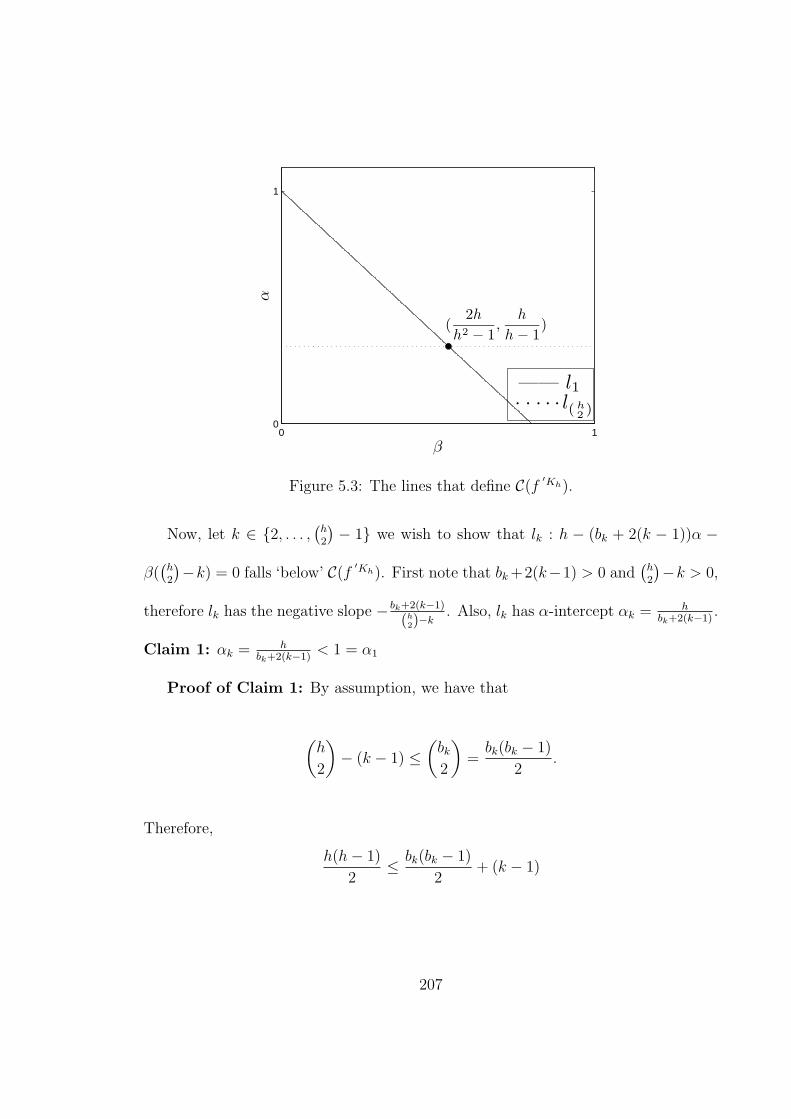
0 10
1
β
α
(2h
h2− 1
,h
h − 1)
· · · · · l( h
2)
—— l1
Figure 5.3: The lines that define C(f′Kh).
Now, let k ∈ {2, . . . , (h2
) − 1} we wish to show that lk : h − (bk + 2(k − 1))α −
β((
h2
)−k) = 0 falls ‘below’ C(f′Kh). First note that bk +2(k−1) > 0 and
(h2
)−k > 0,
therefore lk has the negative slope − bk+2(k−1)
(h2)−k
. Also, lk has α-intercept αk = hbk+2(k−1)
.
Claim 1: αk = hbk+2(k−1)
< 1 = α1
Proof of Claim 1: By assumption, we have that
(h
2
)− (k − 1) ≤
(bk
2
)=
bk(bk − 1)
2.
Therefore,
h(h− 1)
2≤ bk(bk − 1)
2+ (k − 1)
207

and
h(h− 1) ≤ bk(bk − 1) + 2(k − 1).
Now, h ≥ bk since(
bk−12
)<
(h2
)− (k − 1), so
h(h− 1) ≤ bk(h− 1) + 2(k − 1).
Also, h− 1 > 1, hence
h(h− 1) < bk(h− 1) + 2(k − 1)(h− 1)
and so we see that
h
bk + 2(k − 1)< 1.
Hence, αk < α1 and Claim 1 holds.
So, we have that lk has negative slope and α-intercept below that of l1. Since
lk is not a vertical line, we know that lk goes thought the point ( 2hh2−1
, α0) for some
α0. If we can show that α0 < 1h−1
, then the point ( 2hh2−1
, α0) is directly under the
intersection point of l1 and l(h2)
, ( 2hh2−1
, 1h−1
).
Claim 2: lk a goes though the point ( 2hh2−1
, α0) for some α0 < 1h−1
Proof of Claim 2: The line lk is the line h− (bk + 2(k − 1))α− β((
h2
)− k) = 0,
208

therefore when β = 2hh2−1
we have that
h− (bk + 2(k − 1)) α0 − 2h
h2 − 1
((h
2
)− k
)= 0
and it is easy to see that
α0 =2kh
(bk + 2(k − 1))(h + 1)(h− 1).
Now, hh+1
< 1 and so
α0 <2k
(bk + 2(k − 1))(h− 1).
Now, by assumption,(
bk
2
) ≥ (h2
)−(k−1) ≥ 1, therefore bk ≥ 2 and bk +2(k−1) ≥ 2k.
Hence 2kbk+2(k−1)
≤ 1 and so we see that
α0 <1
h− 1
and Claim 2 holds.
Claims 1 and 2 together with the facts that lk has negative slope and l(h2)
is a
horizontal line, ensures that lk is ‘below’ C(f′Kh) for all k ∈ {2, . . . , (h
2
)− 1}.
Hence by Propositions 4.2.3 and 4.2.5 we see that f′Kh
α,β,h(n) can be obtained from
fKhα,β,h(n) by removing each of the terms associated with the lines lk, 2 ≤ k ≤ (
h2
)− 1,
and furthermore f′Kh
α,β,h(n) = f red Khα,β,h (n). Hence f
′Khα,β,h(n) ≡ fKh
α,β,h(n) and so E[ZKh] ≡
f′Kh
α,β,h(n) with E[ZKh] → 0 whenever (β, α) ∈ C(f
′Kh) and E[ZKh] → ∞ whenever
209
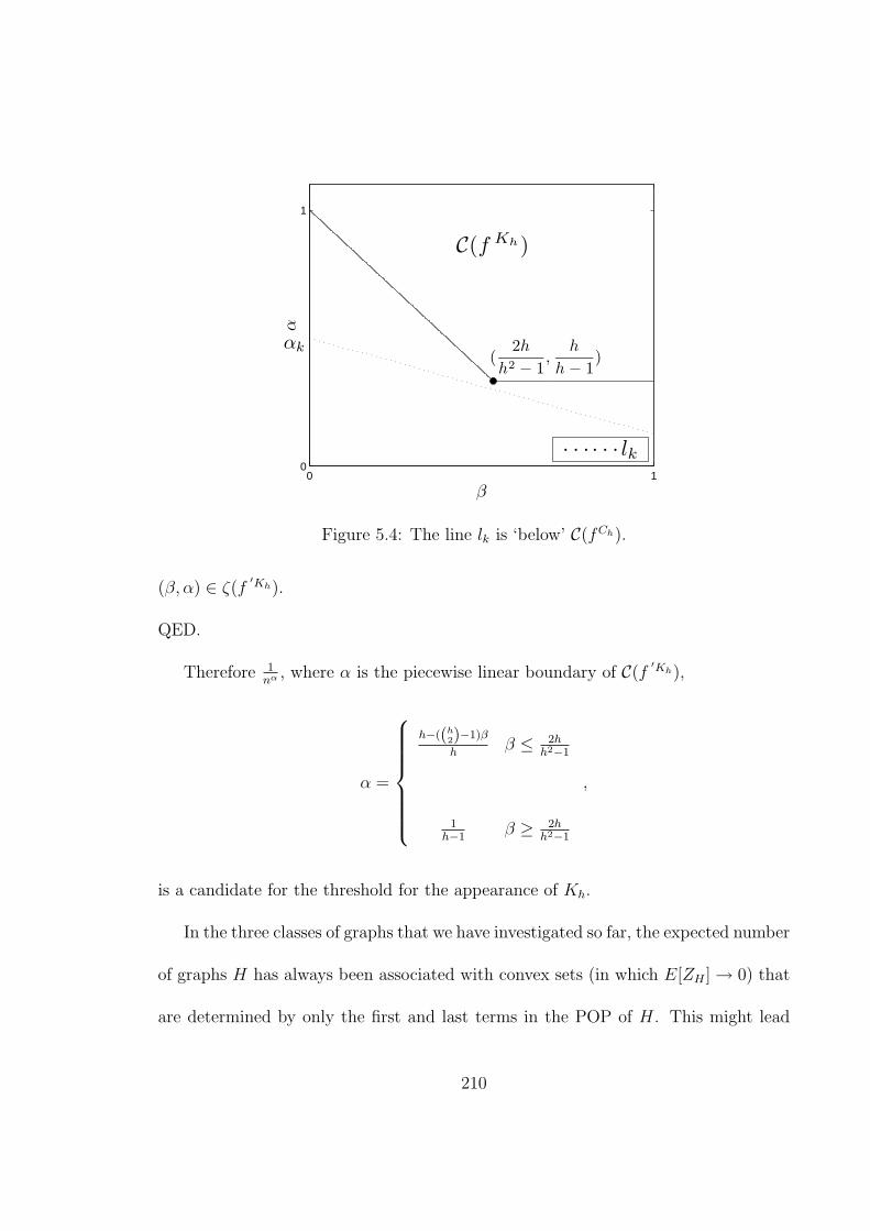
0 10
1
β
α
(2h
h2 − 1,
h
h − 1)
C(f Kh)
αk
· · · · · · lk
Figure 5.4: The line lk is ‘below’ C(fCh).
(β, α) ∈ ζ(f′Kh).
QED.
Therefore 1nα , where α is the piecewise linear boundary of C(f
′Kh),
α =
h−((h2)−1)β
hβ ≤ 2h
h2−1
1h−1
β ≥ 2hh2−1
,
is a candidate for the threshold for the appearance of Kh.
In the three classes of graphs that we have investigated so far, the expected number
of graphs H has always been associated with convex sets (in which E[ZH ] → 0) that
are determined by only the first and last terms in the POP of H. This might lead
210

one to conjecture that this is always the case. However, we show that this conjecture
is false.
Let Hkite be the graph with vertex set V (Hkite) = {v1, v2, v3, v4, v5} and edge set
E(Hkite) = {{v1, v2}, {v1, v3}, {v1, v4}, {v1, v5}, {v2, v3}, {v2, v4}, {v3, v4}}.
Since Hkite is a K4 with a single pendant edge we call Hkite the ‘kite’ graph. See
Figure 5.5.
Figure 5.5: The graph Hkite.
Proposition 5.3.4. Let G be drawn from D[n, {0, 1}t, p] with p = 1nα and t = nβ for
α, β ≥ 0. Let
f′Hkite
α,β,5 (n) = n5−14α + n5−6α−5β + n5−5α−6β.
Then
• the POP of Hkite is gHkite(p, 1/t) = p14 + p13
t+ p11
t2+ p10
t3+ p8
t4+ p6
t5+ p5
t6,
• the expected number of copies of Hkite in G is E[ZHkite] ≡ f
′Hkiteα,β,5 (n) with
211

E[ZHkite] → 0 whenever (β, α) ∈ C(f
′Hkite) and E[ZHkite] → ∞ whenever
(β, α) ∈ ζ(f′Hkite), and
• E[ZHkite] 6≡ n5−14α + n5−5α−6β.
Additionally, the boundary function for C(f′Hkite) is
α =
5−6β5
β ≤ 511
5−5β6
511≤ β ≤ 4
7
514
β ≥ 47
.
Proof:
First, it is easy to show, either directly using Lemma 5.2.5 or by calculating the
POP of K4 by Corollary 5.2.12 and then applying the pendant edge Lemma 5.2.7,
that the POP of Hkite is gHkite(p, 1/t) = p14 + p13
t+ p11
t2+ p10
t3+ p8
t4+ p6
t5+ p5
t6. Therefore,
the expected number of copies of Hkite is G is
E[ZHkite] ³
(n
5
)gHkite
(p, 1/t) ³ fHkiteα,β,5 (n)
= n5−14α + n5−13α−β + n5−11α−2β + n5−10α−3β + n5−8α−4β + n5−6α−5β + n5−5α−6β.
Now, in Figure 5.6 (a) we plot each of the lines associated with the terms in
212
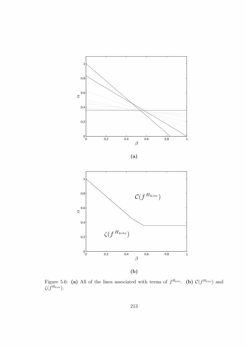
0 0.2 0.4 0.6 0.8 10
0.2
0.4
0.6
0.8
1
β
α
(a)
0 0.2 0.4 0.6 0.8 10
0.2
0.4
0.6
0.8
1
β
α
C(f Hkite)
ζ(f Hkite)
(b)
Figure 5.6: (a) All of the lines associated with terms of fHkite . (b) C(fHkite) andζ(fHkite).
213

fHkiteα,β,5 (n) in the β, α-parameter space. Clearly, the convex region C(fHkite) is deter-
mined by the solid lines associated with the first, last and penultimate terms and that
the dotted lines associated with all of the other terms fall ‘below’ C(fHkite).
Hence by Propositions 4.2.3 and 4.2.5 we see that f′Hkite
α,β,5 (n) can be obtained
from fHkiteα,β,5 (n) by removing each of the terms associated with the dashed lines and
furthermore f′Kh
α,β,h(n) = f red Khα,β,h (n). Therefore
E[ZHkite] ³ fHkite
α,β,5 (n) ≡ f′Hkite
α,β,5 (n) = n5−14α + n5−6α−5β + n5−5α−6β
and hence C(fHkite) = C(f′Hkite). Additionally, since f
′Khα,β,h(n) = f red Kh
α,β,h (n), E[ZHkite] 6≡
n5−14α + n5−5α−6β.
QED.
So the convex set associated with the expected number of copies of Hkite has a
piecewise linear boundary composed of three pieces and not just the two conjectured.
5.3.2 Threshold Theory
We begin this section by presenting a threshold result for K3.
First, recall that by Corollary 5.2.12 that the POP of K3 is gK3(p, 1/t) = p6 +
p5
t+ p3
t2. Also, recall from Proposition 5.3.3 that the expected number of copies of
K3 goes to zero for all (β, α) ∈ C(f′K3) and goes to infinity for all (β, α) ∈ ζ(f
′K3),
where f′K3
α,β,3(n) = n3−3α−2β + n3−6α.
214
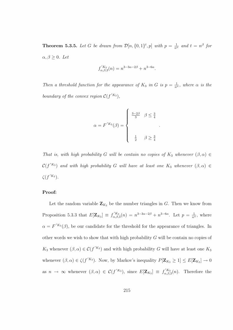
Theorem 5.3.5. Let G be drawn from D[n, {0, 1}t, p] with p = 1nα and t = nβ for
α, β ≥ 0. Let
f′K3
α,β,3(n) = n3−3α−2β + n3−6α.
Then a threshold function for the appearance of K3 in G is p = 1nα , where α is the
boundary of the convex region C(f′K3),
α = F′K3(β) =
3−2β3
β ≤ 34
12
β ≥ 34
.
That is, with high probability G will be contain no copies of K3 whenever (β, α) ∈
C(f′K3) and with high probability G will have at least one K3 whenever (β, α) ∈
ζ(f′K3).
Proof:
Let the random variable ZK3 be the number triangles in G. Then we know from
Proposition 5.3.3 that E[ZK3 ] ≡ f′K3
α,β,3(n) = n3−3α−2β + n3−6α. Let p = 1nα , where
α = F′K3(β), be our candidate for the threshold for the appearance of triangles. In
other words we wish to show that with high probability G will be contain no copies of
K3 whenever (β, α) ∈ C(f′K3) and with high probability G will have at least one K3
whenever (β, α) ∈ ζ(f′K3). Now, by Markov’s inequality P [ZK3 ≥ 1] ≤ E[ZK3 ] → 0
as n → ∞ whenever (β, α) ∈ C(f′K3), since E[ZK3 ] ≡ f
′K3α,β,3(n). Therefore the
215

P [ZK3 = 0] → 1 as n →∞ and almost every graph has no K3.
Also, whenever (β, α) ∈ ζ(f′K3), then E[ZK3 ] →∞ and we use the second moment
method. By Chebychev’s inequality we know that P [X = 0] ≤ Var(ZK3)/E[ZK3 ]2 =
E[Z2K3
]−E[ZK3]2
E[ZK3]2
.
Now, in Section 5.1.2 we showed if a, b, c, u, v, w ∈ V (G), u < v < w, a < b < c,
all distinct vertices, that the first term in the variance calculation is
E[Z2] =
(n
3
)P [the triangle uvw]+
(n
3
)(n−3)3P [{the triangle uvw}∩{the triangle avw}]
+
(n
3
)(n− 3
2
)3P [{the triangle uvw} ∩ {the triangle abw}]
+
(n
3
)(n− 3
3
)P [{the triangle uvw} ∩ {the triangle abc}].
Now, using Lemma 5.2.5 to calculate the POPs of the required graphs in the
equation we see that
E[Z2] ³ E[Zk3 ] + n4(p10 +p9
t+
p7
t2+
p6
t3+
p4
t4) + n5(p12 +
p11
t+
p9
t2+
p8
t3+
p6
t4+
p5
t5)
+
(n
3
)(n− 3
3
)(P [the triangle uvw])2.
Now, let
g∗α,β,4(n) = n4−10α + n4−9α−β + n4−7α−2β + n4−6α−3β + n4−4α−4β
216
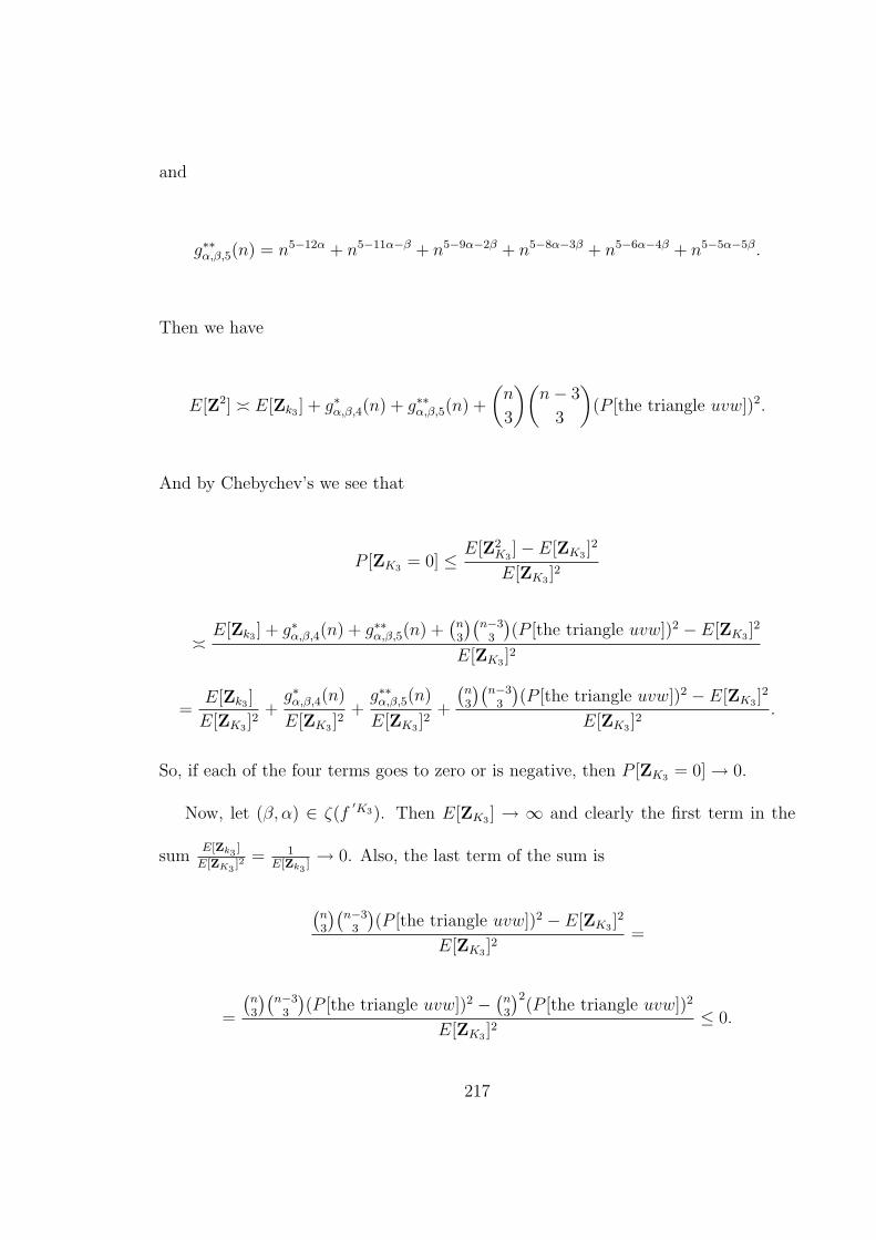
and
g∗∗α,β,5(n) = n5−12α + n5−11α−β + n5−9α−2β + n5−8α−3β + n5−6α−4β + n5−5α−5β.
Then we have
E[Z2] ³ E[Zk3 ] + g∗α,β,4(n) + g∗∗α,β,5(n) +
(n
3
)(n− 3
3
)(P [the triangle uvw])2.
And by Chebychev’s we see that
P [ZK3 = 0] ≤ E[Z2K3
]− E[ZK3 ]2
E[ZK3 ]2
³ E[Zk3 ] + g∗α,β,4(n) + g∗∗α,β,5(n) +(
n3
)(n−3
3
)(P [the triangle uvw])2 − E[ZK3 ]
2
E[ZK3 ]2
=E[Zk3 ]
E[ZK3 ]2
+g∗α,β,4(n)
E[ZK3 ]2
+g∗∗α,β,5(n)
E[ZK3 ]2
+
(n3
)(n−3
3
)(P [the triangle uvw])2 − E[ZK3 ]
2
E[ZK3 ]2
.
So, if each of the four terms goes to zero or is negative, then P [ZK3 = 0] → 0.
Now, let (β, α) ∈ ζ(f′K3). Then E[ZK3 ] → ∞ and clearly the first term in the
sumE[Zk3
]
E[ZK3]2
= 1E[Zk3
]→ 0. Also, the last term of the sum is
(n3
)(n−3
3
)(P [the triangle uvw])2 − E[ZK3 ]
2
E[ZK3 ]2
=
=
(n3
)(n−3
3
)(P [the triangle uvw])2 − (
n3
)2(P [the triangle uvw])2
E[ZK3 ]2
≤ 0.
217

So, if we can show thatg∗α,β,4(n)
E[ZK3]2→ 0 and
g∗∗α,β,5(n)
E[ZK3]2→ 0 then we will have shown that
P [ZK3 = 0] → 0.
Now, recall from the proof of Proposition 5.3.3 that E[ZK3 ] ³ fK3α,β,3(n) = n3−3α−2β+
n3−5α−β + n3−6α and that fK3α,β,3(n) ≡ f
′K3α,β,3(n). So we see that E[ZK3 ]
2 ³ (fK3α,β,3(n))2
and, noting that all of the coefficients of α are distinct and increasing as the coeffi-
cients of β decrease, we use Proposition 4.2.6 to yield
E[ZK3 ]2 ³ (fK3
α,β,3(n))2 ≡ fK3α,β,3(n) ≡ f
′K3α,β,3(n).
Hence the convex set associated with E[ZK3 ]2 is the same as the set associated with
E[ZK3 ], i.e., C(f′K3).
We show thatg∗α,β,4(n)
E[ZK3]2→ 0 and
g∗∗α,β,5(n)
E[ZK3]2→ 0. First let us consider
g∗α,β,4(n)
E[ZK3]2³
g∗α,β,4(n)
(fK3α,β,3(n))2
. By Theorem 4.3.5g∗α,β,4(n)
(fK3α,β,3(n))2
→ 0 if all of the lines associated with the
terms of g∗α,β,4(n) are ‘below’ C((fK3)2) = C(f′K3).
It is easy to see by Figure 5.7 that this is indeed the case. Therefore
g∗α,β,4(n)
E[ZK3 ]2³ g∗α,β,4(n)
(fK3α,β,3(n))2
→ 0
for all (β, α) ∈ ζ(f′K3).
218

0 0.2 0.4 0.6 0.8 10
0.2
0.4
0.6
0.8
1
β
αC(f
′K3)
ζ(f′K3)
Figure 5.7: The dotted lines are those associated with terms of g∗α,β,4(n) and are all
‘below’ C(f′K3).
Also, by an argument similar to that above and Figure 5.8, we see that
g∗∗α,β,5(n)
E[ZK3 ]2³ g∗∗α,β,5(n)
(fK3α,β,3(n))2
→ 0
for all (β, α) ∈ ζ(f′K3).
So, P [ZK3 = 0] → 0 as n → ∞ whenever (β, α) ∈ ζ(f′K3) and almost every
graph contains a K3. Hence a threshold function for the appearance of K3 in G is
the boundary of the convex region C(f′K3).
QED.
We would like to prove a general threshold result, however without a result for
the POP of a general graph, we have as yet been unable. Instead we present a result
219

0 0.2 0.4 0.6 0.8 10
0.2
0.4
0.6
0.8
1
β
αC(f
′K3)
ζ(f′K3)
Figure 5.8: The dotted lines are those associated with terms of g∗∗α,β,5(n) and are all
‘below’ C(fK3).
that gives a method to prove threshold results when the threshold is the boundary
of the associated convex set and all required POPs are known. But first, we prove a
lemma that allows us to use Proposition 4.2.6.
Lemma 5.3.6. Let H be a connected graph with |E(H)| = m edges. Let
gH(p, 1/t) = px0 +px1
t+
px2
t2+ · · ·+ pxm−2
tm−2+
pxm−1
tm−1
be the POP of H. Let i, j ∈ {0, 1, . . . , m− 1}. If i < j then xi > xj.
Proof:
By Lemma 5.2.5 for all 0 ≤ j ≤ m − 1, xj = hm−j is the minimum number of
vertices used in a graph induced by a partition of the edge set into of m − j parts.
220

Additionally, Lemma 5.2.10 tells us that whenever i < j, xi = hm−i > hm−j = xj.
QED.
Theorem 5.3.7. Let G be drawn from D[n, {0, 1}t, p] with p = 1nα and t = nβ for
α, β ≥ 0. Let H be a connected graph with |V (H)| = h vertices and |E(H)| = m
edges. Let
gH(p, 1/t) = px0 +px1
t+
px2
t2+ · · ·+ pxm−2
tm−2+
pxm−1
tm−1
be the POP of H. Let fHα,β,h(n) =
∑m−1i=0 nh−xiα−βi and C(fH) be the convex region in
which fHα,β,h(n) → 0 as described in Proposition 4.1.1.
Let H be the set of all graphs that can be formed by merging two copies of H. For
any A ∈ H, let hA = |V (A)| and mA = |E(A)|. Also, suppose that the POP of A is
gA(p, 1/t) = px(A)0 +px(A)1
t+
px(A)2
t2+ · · ·+ px(A)mA−2
tmA−2+
px(A)mA−1
tmA−1.
Let fAα,β,hA
(n) =∑mA−1
i=0 nhA−x(A)iα−βi. Finally, for all 0 ≤ i ≤ mA − 1, let l(A)i :
hA − x(A)iα− βi = 0 be the line associated with the ith term in the sum fAα,β,hA
(n).
If for all A ∈ H with h < |V (A)| < 2h, all of the lines l(A)i, 0 ≤ i ≤ mA, are
‘below’ C(fH) then a threshold function for the appearance of H in G is p = 1nα , where
α = FH(β) is the boundary of the convex region C(fH). That is as n →∞, with high
probability G will contain no copies of H whenever (β, α) ∈ C(fH) and G will have
at least one copy of H whenever (β, α) ∈ ζ(fH).
221
Proof:
Let ZH be the number of copies of H in G. Then, as discussed in section Section
5.3.1, E[ZH ] ³ ∑m−1i=0 nh−xiα−βi = fH
α,β,h(n). Then Proposition 4.1.1 implies that
E[ZH ] → 0 whenever (β, α) ∈ C(fH) and E[ZH ] → ∞ whenever (β, α) ∈ ζ(fH).
Hence, the piecewise linear boundary function α = FH(β) is a our candidate for the
threshold of the appearance of H in G.
Now, by Markov’s inequality P [ZH ≥ 1] ≤ E[ZH ] → 0 as n → ∞ whenever
(β, α) ∈ C(fH). Therefore P [Z = 0] → 1 and almost no G contains H whenever
(β, α) ∈ C(fH).
Also, whenever (β, α) ∈ ζ(fH), E[ZH ] → ∞ as n → ∞ and we use the second
moment method. By Chebychev’s inequality we know that
P [ZH = 0] ≤ Var(ZH)
E[ZH ]2=
E[Z2H ]− E[ZH ]2
E[ZH ]2
and so, we calculate E[Z2H ] and E[ZH ]2.
Now, for all A ∈ H let ZA be the number of copies of A in G. Then we claim that
E[Z2H ] = E[
∑A∈H ZA].
Let B be the set of all graphs that lie on a subset of the vertex set of G and are
isomorphic to H. Then for each B ∈ B, let IB be the indicator that B ⊆ G. Then
222

ZH =∑
B∈B IB and
E[Z2H ] = E
(∑B∈B
IB
)2 = E
[(∑B∈B
IB
)( ∑B∗∈B
IB∗
)]= E
[ ∑B,B∗∈B
IB IB∗
].
Now, IB IB∗ is equal to 1 if and only if both B and B∗ appear in G, i.e. if and only
if B⋃
B∗ appears in G. Therefore, IB IB∗ = IBS
B∗ where IBS
B∗ is the indicator
function for the graph B⋃
B∗ in G.
Hence
E[Z2H ] = E
[ ∑B,B∗∈B
IB∪B∗
]= E
∑A∈H
∑
B,B∗∈BBS
B∗=A
IB∪B∗
=
∑A∈H
E
∑
B,B∗∈BBS
B∗=A
IB∪B∗
=∑A∈H
∑
B,B∗∈BBS
B∗=A
E[IB∪B∗ ] =∑A∈H
∑
B,B∗∈BBS
B∗=A
P≥[B ∪B∗] =∑A∈H
∑
B,B∗∈BBS
B∗=A
P≥[A]
=∑A∈H
∑
B,B∗∈BBS
B∗=A
E[IA] =∑A∈H
E
∑
B,B∗∈BBS
B∗=A
IA
=
∑A∈H
E[ZA]
and our claim is true. Thus, E[Z2H ] = E[
∑A∈H ZA].
Now,
E[Z2H ] =
∑A∈H
E[ZA] =∑A∈H
|V (A)|=h
E[ZA] +∑A∈H
h+1≤|V (A)|=2h−1
E[ZA] +∑A∈H
|V (A)|=2h
E[ZA].
If |V (A)| = h, then A = H and so∑
A∈H|V (A)|=h
E[ZA] = E[ZH ]. Also, if |V (A)| = 2h
223

then A is the graph that contains two disjoint copies of H and so∑
A∈H|V (A)|=2h
E[ZA] =
(nh
)(n−h
h
)P≥[H]2. So, we have that
E[Z2H ] = E[ZH ] +
∑A∈H
h+1≤|V (A)|=2h−1
E[ZA] +
(n
h
)(n− h
h
)P≥[H]2.
Therefore Chebychev’s inequality becomes
P [ZH = 0] ≤E[ZH ] +
∑A∈H
h+1≤|V (A)|=2h−1E[ZA] +
(nh
)(n−h
h
)P≥[H]2 − E[ZH ]2
E[ZH ]2
=E[ZH ]
E[ZH ]2+
∑A∈H
h+1≤|V (A)|=2h−1E[ZA]
E[ZH ]2+
(nh
)(n−h
h
)P≥[H]2 − E[ZH ]2
E[ZH ]2.
Now, let us consider each of the three terms separately. The first term E[ZH ]E[ZH ]2
→ 0
whenever (β, α) ∈ ζC(fH) since E[ZH ] →∞. Also, the last term is
(nh
)(n−h
h
)P≥[H]2 − E[ZH ]2
E[ZH ]2=
(nh
)(n−h
h
)P≥[H]2 − (
nh
)2P≥[H]2
E[ZH ]2≤ 0.
Therefore, if we can show that the middle term
(∑A∈H
h+1≤|V (A)|=2h−1E[ZA]
)/E[ZH ]2 →
0 whenever (β, α) ∈ C(fH), then P [ZH = 0] → 0 and we will be done.
Now, there are only a finite number of A ∈ H. Therefore if we can show that
for all A ∈ H with h + 1 ≤ |V (A)| = 2h − 1,we have E[ZA]/E[ZH ]2 → 0 then(∑
A∈Hh+1≤|V (A)|=2h−1
E[ZA]
)/E[ZH ]2 → 0.
224
So, let A ∈ H with h + 1 ≤ |V (A)| = 2h− 1, then as discussed in Section 5.3.1
E[ZA] ³(
n
hA
)gA(p, 1/t) ³
mA−1∑i=0
nhA−x(A)iα−βi = fAα,β,hA
(n)
and so E[ZA]/E[ZH ]2 → 0 if and only if fAα,β,hA
(n)/E[ZH ]2 → 0.
Now, E[ZH ] ³ fHα,β,h(n) =
∑m−1i=0 nh−xiα−βi and so
E[ZH ]2 ³ (fHα,β,h(n))2 =
(m−1∑i=0
nh−xiα−βi
)2
=m−1∑i,j=0
n2h−(xi+xj)α−β(i+j)
and is a posynomial of the form discussed in Chapter 4.
Furthermore, whenever (β, α) ∈ ζ(fH), (fHα,β,h(n))2 →∞ and
E[ZA]
E[ZH ]2³ fA
α,β,hA(n)
(fHα,β,h(n))2
=
∑mA−1i=0 nhA−x(A)iα−βi
∑m−1i,j=0 n2h−(xi+xj)α−β(i+j)
is a ratio of the form2 discussed in Theorem 4.3.5 since hA < 2h. So, E[ZA]E[ZH ]2
→ 0 if
for each 0 ≤ i ≤ mA, li is ’below’ C((fH)2).
Finally, by Lemma 5.3.6, we have that xi > xj when i < j , and so by Proposition
4.2.6 we have that (fHα,β,h(n))2 ≡ fH
α,β,h(n) and so C((fH)2) = C(fH). Therefore
E[ZA]E[ZH ]2
→ 0 if for each 0 ≤ i ≤ mA, li is ’below’ C(fH).
Hence, if for all A ∈ H with h < |V (A)| < 2h all of the lines l(A)i, 0 ≤ i ≤ mA,
are ‘below’ C(fH) then P [ZH = 0] → 0 as n → ∞ whenever (β, α) ∈ ζ(fH) and
2While it is true that the upper limits on the sums do not agree, this can easily be fixed bysetting both upper limits to some M that is larger than both (m − 1)2 and mA and then addingterms equal to 0 to fill out the summation.
225

almost every G will contain a copy of H.
Therefore, if for all A ∈ H with h < |V (A)| < 2h, all of the lines l(A)i, 0 ≤ i ≤ mA,
are ‘below’ C(fH), then, as n →∞, with high probability G will be contain no copies
of H whenever (β, α) ∈ C(fH) and G will have at least one copy of H whenever
(β, α) ∈ ζ(fH). So a threshold function for the appearance of H in G is α = FH(β),
the boundary of the convex region C(fH).
QED.
Theorem 5.3.7 gives us a method to prove threshold results if the boundary of
the convex region associated with the graph is indeed the threshold and all needed
POPs are known. This might cause one to conjecture that the boundary is always
the threshold, but this is not the case.
Consider the kite graph Hkite discussed in Section 5.3.1. By Proposition 5.3.4 we
know that the boundary function for C(f′Hkite) = C(fHkite) is
α =
5−6β5
β ≤ 511
5−5β6
511≤ β ≤ 4
7
514
β ≥ 47
and E[Zkite] → 0 whenever (β, α) ∈ C(f′Hkite) and E[Zkite] → ∞ whenever (β, α) ∈
ζ(f′Hkite). However p = 1
nα is not the correct threshold.
226

First we show that Hkite does not satisfy all of the conditions of Theorem 5.3.7.
Consider the graph H2−kite with vertex set V (H2−kite) = {v1, v2, v3, v4, v5, v6} and
edge set
E(H2−kite) = {{v1, v2}, {v1, v3}, {v1, v4}, {v1, v5}, {v2, v3}, {v2, v4}, {v3, v4}, {v3, v6}}.
H2−kite is a K4 with two pendant edges attached to different vertices, see Figure
5.9. Also, H2−kite is a graph that can be formed by merging to copies of Hkite, i.e.,
H2−kite ∈ Hkite.
Figure 5.9: The graph H2−kite.
It is easy to show, either directly using Lemma 5.2.5 or by applying the pendant
edge Lemma 5.2.7 to the POP of Hkite, that the POP of H2−kite is gH2−kite(p, 1/t) =
p16 + p15
t+ p13
t2+ p12
t3+ p10
t4+ p8
t5+ p7
t6+ p6
t7. Therefore, the expected number of copies of
Hkite in G is
E[ZH2−kite] ³
(n
6
)gH2−kite
(p, 1/t) ³ fH2−kite
α,β,6 (n)
= n6−16α+n6−15α−β+n6−13α−2β+n6−12α−3β+n6−10α−4β+n6−8α−5β+n6−7α−6β+n6−6α−7β.
227
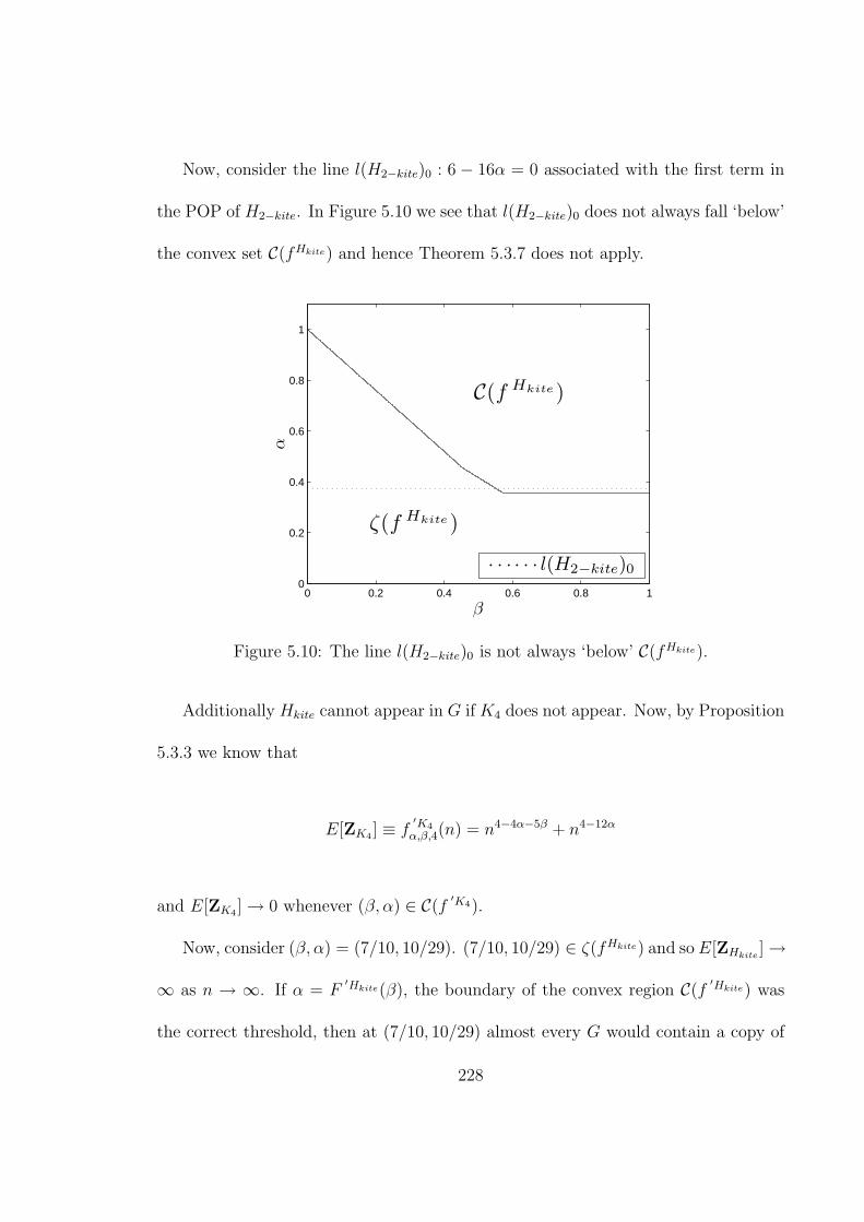
Now, consider the line l(H2−kite)0 : 6 − 16α = 0 associated with the first term in
the POP of H2−kite. In Figure 5.10 we see that l(H2−kite)0 does not always fall ‘below’
the convex set C(fHkite) and hence Theorem 5.3.7 does not apply.
0 0.2 0.4 0.6 0.8 10
0.2
0.4
0.6
0.8
1
β
α
C(f Hkite)
ζ(f Hkite)
· · · · · · l(H2−kite)0
Figure 5.10: The line l(H2−kite)0 is not always ‘below’ C(fHkite).
Additionally Hkite cannot appear in G if K4 does not appear. Now, by Proposition
5.3.3 we know that
E[ZK4 ] ≡ f′K4
α,β,4(n) = n4−4α−5β + n4−12α
and E[ZK4 ] → 0 whenever (β, α) ∈ C(f′K4).
Now, consider (β, α) = (7/10, 10/29). (7/10, 10/29) ∈ ζ(fHkite) and so E[ZHkite] →
∞ as n → ∞. If α = F′Hkite(β), the boundary of the convex region C(f
′Hkite) was
the correct threshold, then at (7/10, 10/29) almost every G would contain a copy of
228

Hkite. However, (7/10, 10/29) ∈ C(fK4)and so E[ZK4 ] → 0 as n → ∞. Therefore,
by Markov’s inequality, P [Zk4 ≥ 1] ≤ E[Zk4 ] → 0 and almost no G contains a K4.
Hence, almost no G contains a Hkite. Therefore, the boundary of the convex region
is not the correct threshold.
0 0.2 0.4 0.6 0.8 10
0.2
0.4
0.6
0.8
1
β
α
C(f Hkite)
ζ(f Hkite)
0 0.2 0.4 0.6 0.8 10
0.2
0.4
0.6
0.8
1
β
α
C(f K4)
ζ(f K4)
(a) (b)
Figure 5.11: (a) The point (7/10, 10/29) ∈ C(fHkite). (b) The point (7/10, 10/29) ∈ζ(fK4).
Although we have been unable to prove a more general threshold result, we make
the following conjectures.
Conjecture 5.3.8. Let G be drawn from D[n, {0, 1}t, p] with p = 1nα and t = nβ for
α, β ≥ 0. Let H be a connected graph and H∗ be the set of all non empty subgraphs
of H. Let ΛH be the region in the β, α-parameter space in which for all H∗ ∈ H∗,
E[ZH∗ ] →∞ as n →∞. Then the threshold for the appearance of H is the boundary
of ΛH .
Recall from Section 3.2.1, for any graph H on k vertices and l ≥ 1 edges, ε(H) = lk.
229

We say that H is strictly balanced if for every proper subgraph H ′ of H, ε(H ′) < ε(H).
We make the following conjecture about the threshold for the appearance of a strictly
balanced graph H as a subgraph of a Discrete Random Dot Product Graph.
Conjecture 5.3.9. Let G be drawn from D[n, {0, 1}t, p] with p = 1nα and t = nβ for
α, β ≥ 0. Let H be a connected graph with |V (H)| = h vertices and |E(H)| = m
edges. Let
gH(p, 1/t) = px0 +px1
t+
px2
t2+ · · ·+ pxm−2
tm−2+
pxm−1
tm−1
be the POP of H. Let fHα,β,h(n) =
∑m−1i=0 nh−xiα−βi and α = FH(β) be the boundary
of the convex region in which fHα,β,h(n) → 0 as described in Proposition 4.1.1. If H is
strictly balanced, then a threshold function for the appearance of H in G is p = 1nα .
230

Chapter 6
Overview and Directions for
Future Work
In this thesis we introduce and examine the Random Dot Product Graph suite
of models. Three sets of models for social networks are presented, all based on the
idea of common or shared interest. The first model, discussed in Chapter 2, is the
Dense Random Dot Product Graph. In this model, all small subgraphs appear with
probability approaching one as the number of vertices approaches infinity. The second
model, discussed in Chapter 3, is the Sparse Random Dot Product Graph and small
subgraphs appear at certain thresholds. Finally, the third model is a discrete version
and is discussed in Chapter 5. As in the sparse model, in the Discrete Random Dot
Product Graph small subgraphs appear at various thresholds.
In this chapter, we revisit each of the models, review our results and suggest
231
ideas for further work. Then in the last section we discuss more general ideas and
directions.
6.1 Observations and New Directions
In this section, we recap the main results and pose open questions related to each
of the individual models.
6.1.1 The Dense Random Dot Product Graph
In Chapter 2 we introduce the general Random Dot Product Graph. We then
focus on the Dense model for the dimension one case, i.e. when G is drawn from
D[n, a, 1]. In Section 2.2.1, we show that the expected number of edges is(
n2
)1
(a+1)2
and for a fixed k, the expected number of vertices of degree k, denoted λ(k), is
E[λ(k)] ∼(
1k! a
(1 + a)1a Γ
(1a
+ k))
na−1
a as n → ∞. However, we do not present the
variance calculations, the next logical step, and so we pose the questions:
• How close to expected are these values?
• If we allow 0 < a ≤ 1, then for what k do we, with high probability, have
vertices of degree k, i.e., what is the threshold (in terms of a) for the appearance
of vertices of degree k?
In Section 2.3.1, we show that the model obeys the degree distribution power law.
However, we do not directly prove Conjecture 2.3.1 and hence it is left for future
232

work.
In Sections 2.3.2 and 2.3.3 we show that the Dense Random Dot Product Graph
exhibits clustering and has a low fixed diameter of at most six as n →∞. Also, recall,
by the definition presented in Section 1.2.4, that a small world graph is a graph G on n
vertices with average degree k for which LG ≈ LR(n,k) ≈ log(n)log(k)
, but γG À γR(n,k) ≈ kn,
that is a graph for which the characteristic path length is small and similar to that
of a random graph, but whose vertices are highly clustered.
For the Dense Random Dot Product Graph drawn from D[n, a, 1] the expected
average degree is E[k] = (n− 1)/(a + 1)2. So, by small world standards, G would be
highly clustered if it’s clustering coefficient γG À n−1n(a+1)2
and we posit the following:
Conjecture 6.1.1. Let G be drawn from D[n, a, 1]. Then P (γG À 1(a+1)2
) tends to 1
as n →∞.
Empirical results support this conjecture, as does our clustering result Lemma
2.3.6. The other main characteristic of a small world graph is that the characteristic
path length LG is approximately that of the random graph R(n, k), where LR(n, k) ≈log(n)
log“
n+1(a+1)2
” ≈ 1 for large n. Ignoring vertices of degree zero, our diameter result,
Theorem 2.3.9, has shown that for G drawn from D[n, a, 1] one has LG = θ(1).
Towards the end of Chapter 2, we extend the Dense Random Dot Product Graph
into higher dimensions, i.e., consider the case when G is drawn from D[n, a, t], (t > 0).
We prove some results similar to those in a single dimension. We again show that
the expected number of isolated vertices is(
n2
)/(a + 1)2 and is not dependent on the
233
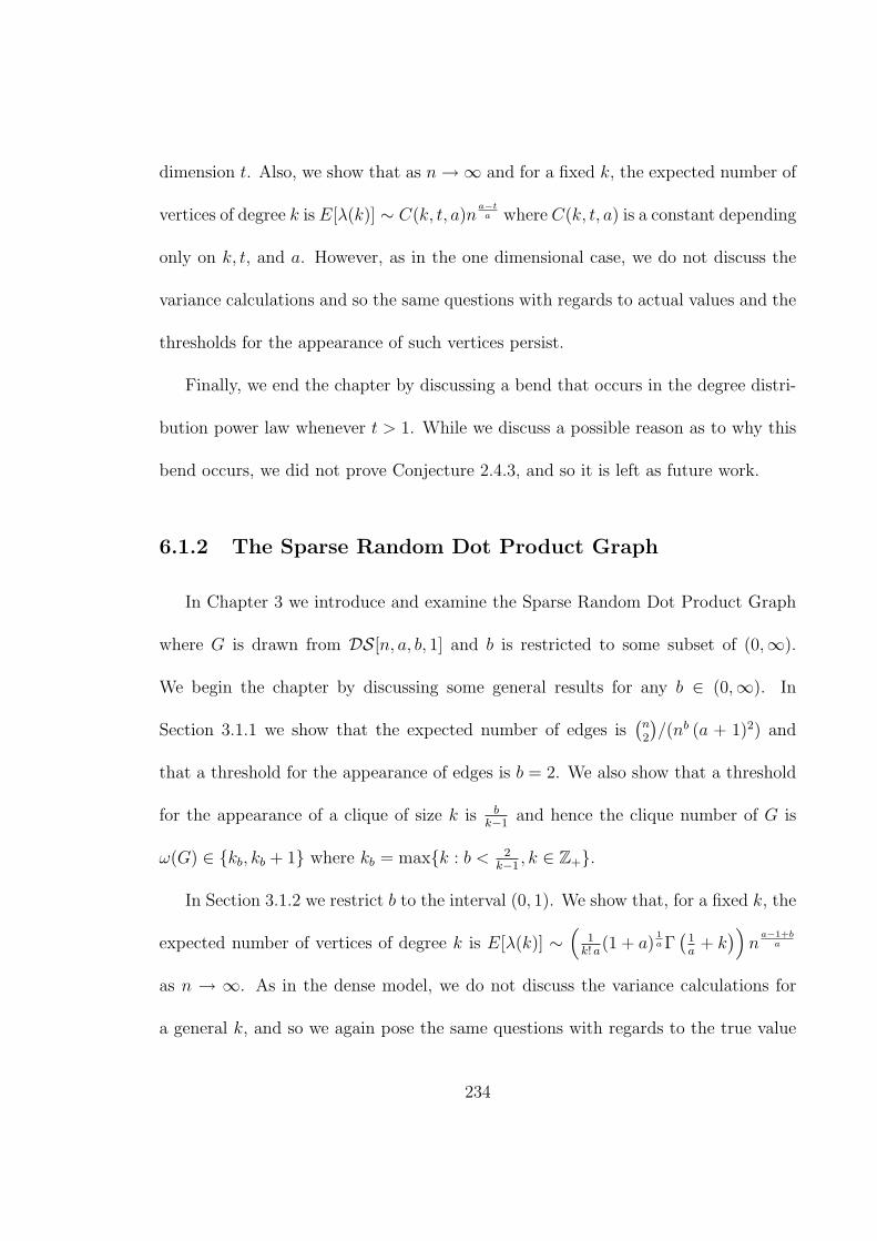
dimension t. Also, we show that as n →∞ and for a fixed k, the expected number of
vertices of degree k is E[λ(k)] ∼ C(k, t, a)na−t
a where C(k, t, a) is a constant depending
only on k, t, and a. However, as in the one dimensional case, we do not discuss the
variance calculations and so the same questions with regards to actual values and the
thresholds for the appearance of such vertices persist.
Finally, we end the chapter by discussing a bend that occurs in the degree distri-
bution power law whenever t > 1. While we discuss a possible reason as to why this
bend occurs, we did not prove Conjecture 2.4.3, and so it is left as future work.
6.1.2 The Sparse Random Dot Product Graph
In Chapter 3 we introduce and examine the Sparse Random Dot Product Graph
where G is drawn from DS[n, a, b, 1] and b is restricted to some subset of (0,∞).
We begin the chapter by discussing some general results for any b ∈ (0,∞). In
Section 3.1.1 we show that the expected number of edges is(
n2
)/(nb (a + 1)2) and
that a threshold for the appearance of edges is b = 2. We also show that a threshold
for the appearance of a clique of size k is bk−1
and hence the clique number of G is
ω(G) ∈ {kb, kb + 1} where kb = max{k : b < 2k−1
, k ∈ Z+}.
In Section 3.1.2 we restrict b to the interval (0, 1). We show that, for a fixed k, the
expected number of vertices of degree k is E[λ(k)] ∼(
1k! a
(1 + a)1a Γ
(1a
+ k))
na−1+b
a
as n → ∞. As in the dense model, we do not discuss the variance calculations for
a general k, and so we again pose the same questions with regards to the true value
234

of λ(k) and thresholds. However, we do present a variance result for the case k = 0,
when we are concerned with the number of isolated vertices. We show that with
probability tending to one as n → ∞, G always has isolated vertices and hence is
never connected. We also show that the sparse model exhibits clustering.
In Section 3.1.3 we begin by presenting a general result relating the number of
edges in a fixed graph to the probability of the graph appearing as a subgraph of
G. Specifically, we show that for a graph H, the probability of H appearing as a
(not necessarily induced) subgraph of a Sparse Random Dot Product Graph G is
C(H)nmb where m is the number of edges in H and C(H) is a constant depending only
on the graph H. Next we show that a threshold for the appearance of a tree on k
vertices is b = kk−1
. Finally, we restrict b to the interval (1, 2) and show that with
high probability G contains no cycles and therefore is a forest on trees of size bb−1
or
less.
In Section 3.2 we present the main results for the Sparse Random Dot Product
Graph. In Section 3.2.1 we show that for a graph H on k vertices and l ≥ 1 edges,
a threshold for the appearance of H is b = 1ε′(H)
. In Section 3.2.2, we show the
Sparse Random Dot Product Graph obeys the degree distribution power law whenever
b ∈ (0, 1). Additionally, we know that, with high probability, G is edgeless when b > 2
and so we pose the question:
• Can we describe the degree distribution of G when b ∈ [1, 2]?
In Section 3.2.3 we show that when 0 < b < 2a+2
, the Sparse Random Dot Product
235

Graph contains isolated vertices with the remaining vertices connected in a giant
component of diameter at most db = b 11−2ε−b
c+ 5. This leads us to ask the following
questions for b ∈ [ 2a+2
, 2]:
• If we ignore isolated vertices, how many components will G contain?
• Can we characterize the distribution on the orders of the components of G?
• Are we guaranteed isolated edges?
• What is the average path length between two vertices in a component of G?
Finally, in Section 3.3 we recap the sparse model and present the following evolu-
tion for the appearance of subgraphs of order k as b goes from zero to infinity:
• beginning at b = 0 all subgraphs on k vertices are present,
• at b = 2k−1
cliques of size k disappear,
• at b = 1 k-cycles disappear,
• at b = kk−1
trees on k vertices disappear,
• for b > kk−1
there are no connected subgraphs on k vertices, and
• for b > 2 there are no edges in the graph.
Another area of exploration for the Sparse Random Dot Product Graph, is to
extend the model to higher dimensions. A first step would be to mimic the extension
in the Dense case.
236

6.1.3 The Discrete Random Dot Product Graph
We begin Chapter 5 by introducing the Discrete Random Dot Product Graph,
when G is drawn from D[n, {0, 1}t, p], and proving a few basic results. We show that
the probability of an edge is p2 and that threshold for the appearance of edges is
p = 1/n and is independent of the dimension t from which the vectors are drawn. We
also show that whenever p < 1, G exhibits clustering.
In Section 5.1.2 we use K3 as an example to demonstrate the difficulty of cal-
culations in the discrete model. We determine the probability of K3 appearing as a
subgraph and give the equation for the variance of the number of triangles, illustrating
the dependence on both p and the dimension t.
In Section 5.2 we introduce the probability order polynomial (POP) of a graph,
gH(p, 1/t), as a function of p and 1/t that is asymptotic to P≥[H], the probability
of H appearing as a (not necessarily induced) subgraph of a Discrete Random Dot
Product Graph G. We show that for a graph H on m edges, P≥[H] ³ gH(p, 1/t) =
px0 + px1
t+ px2
t2+ · · · + pxm−2
tm−2 + pxm−1
tm−1 where for all 0 ≤ j ≤ m − 1, xj = hm−j is the
minimum number of vertices used in a graph induced by a partition of the edge set
into m − j parts. We then give formulas to calculate the POP of trees, cycles, and
complete graphs. However we are, as of yet, unable to give an effective formula for a
general graph H and so this is left as future work.
In an effort to obtain such a formula for a general graph, a first step could be to
develop an algorithm to partition the edge set of a graph H into parts that induce
237

graphs that use the minimum number of vertices so that Lemma 5.2.5 can be applied.
The obvious algorithms such a greedy approach do not produce the desired partition
in all cases. So, we pose the question:
• Can we develop an efficient algorithm to partition the edge set of a graph into
parts that satisfy the conditions of Lemma 5.2.5?
The results in Section 5.3 rely heavily on the framework built in Chapter 4. We
present first moment results for trees, cycles, and complete graphs. The methods
used in these proofs can easily be expanded to any graph for which the POP is
known. In our examples, the boundary of the region C is always determined by the
lines associated with the first and last terms of the POP. However, we present a
counterexample to this always being the case. So, we asked the question:
• When is the boundary of C determined by only the first and last terms of the
POP?
This will only happen if the line associated with one of the middle terms is ‘above’
the intersection point of the lines associated with the first and last terms. So, we offer
the following conjecture.
Conjecture 6.1.2. Let G be drawn from D[n, {0, 1}t, p] with p = 1nα and t = nβ for
α, β ≥ 0. Let H be a connected graph on h vertices and m edges with POP
gH(p, 1/t) = px0 +px1
t+
px2
t2+ · · ·+ pxm−2
tm−2+
pxm−1
tm−1.
238

Let l0 and lm−1 be the lines associated with the first and last terms, respectively, of
the POP of H. If for all i ∈ {1, . . . , m− 2}, 2mh−hxi
2mi≤ 2m−h
m−1, then the boundary of C
will be determined by only l0 and lm−1 and hence be
α =
h−(m−1)βh
β ≤ 2mh−h2
2m(m−1)
h2m
β ≥ 2mh−h2
2m(m−1)
where 2mh−h2
2m(m−1)is the β coordinate of the intersection point of l0 and lm−1.
In Section 5.3.2, we present a threshold result for K3 and in Theorem 5.3.7 describe
a general method for proving threshold results if all required POPs are known. We
also present an example of a graph that does not meet the requirements of Theorem
5.3.7 and so there is more work to be done. Finally, in Conjecture 5.3.8, we state that
if H is a connected graph and H∗ is the set of all non empty subgraphs of H. Then
we believe that ΛH , the region in the β, α-parameter space in which for all H∗ ∈ H∗,
E[ZH∗ ] →∞ as n →∞ is a threshold for the appearance of H.
Although in Chapter 5 we present a good foundation of theory, many questions
are still left unanswered for the Discrete Random Dot Product Graph. In addition
to new questions similar to those that arise in the other two versions of the model,
there are results that were proven for those versions that remain open for the discrete
case. For example:
• What is the degree distribution?
239

• When are we guaranteed isolated vertices?
• Is the graph connected and if so, what is the diameter?
• What is the evolution of the appearance of various subgraph?
6.2 Other Open Problems and Thoughts for Fu-
ture Work
In this section we present more open questions that are not necessarily specific to
a single version of the model.
6.2.1 General Graph Theory Questions
There are many graph theoretic questions that remain unanswered. For example
in each of the versions of the model:
• If we ignore isolated vertices, what is the connectivity of the remaining compo-
nents?
• What are the graph theoretic invariants, such as clique number, independence
number, domination number, chromatic number, maximum degree, etc.?
240

6.2.2 Variations on the Model
So far in the continuous versions of the model, we have only discussed the basic
Random Dot Product Graph in which the probability mapping f has been the identity
mapping, f(x) = x in the dense case, or f(x) = xnb in the sparse case, and the vectors
are drawn from Ua[0, 1], powers of the uniform distribution on [0, 1]. The model can
be further explored by drawing the vectors from a variety of other distributions or by
changing the probability mapping. The distribution Ua[0, 1] is the same as the Beta
distribution B( 1a, 1). Therefore a natural next step is to draw the vectors from other
Beta distributions. Also, there are the only limitations placed on the probability
mapping is that f : R→ [0, 1], and a variety of other functions meet this criteria, e.g.
f(x) = 1π
tan−1 x + 12, f(x) = 1
2tanh x + 1
2, and f(x) = 1− e−x2
. However, one should
note that the nature of these suggested functions may make the work intractable.
Similarly, in the discrete case, changing the probability mapping, perhaps to
f(x) = xnbt
, will change the model and open up new avenues of research.
Variations can also be made upon the way in which we extend the dense model
into higher dimensions. The current method allows the vectors to be drawn from the
first orthant portion of a box centered at the origin. This model does not include all
vector values x and y, whose dot product x ·y ≤ 1. Perhaps another way of extending
the model would be to let f(x ·y) = |x ·y| or f(x ·y) = (x ·y)2 and then study vectors
drawn from an origin centered ball of radius 1 instead. Or, more simply and keeping
with the original box idea, we can draw each vector x from [Ua[0, r]]t instead of just
241
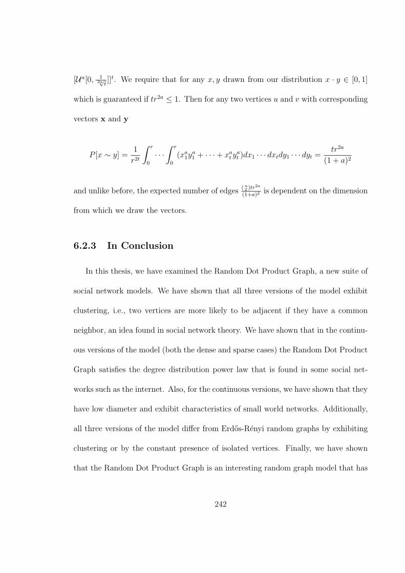
[Ua[0, 12a√t
]]t. We require that for any x, y drawn from our distribution x · y ∈ [0, 1]
which is guaranteed if tr2a ≤ 1. Then for any two vertices u and v with corresponding
vectors x and y
P [x ∼ y] =1
r2t
∫ r
0
· · ·∫ r
0
(xa1y
a1 + · · ·+ xa
t yat )dx1 · · · dxtdy1 · · · dyt =
tr2a
(1 + a)2
and unlike before, the expected number of edges( n2 )tr2a
(1+a)2is dependent on the dimension
from which we draw the vectors.
6.2.3 In Conclusion
In this thesis, we have examined the Random Dot Product Graph, a new suite of
social network models. We have shown that all three versions of the model exhibit
clustering, i.e., two vertices are more likely to be adjacent if they have a common
neighbor, an idea found in social network theory. We have shown that in the continu-
ous versions of the model (both the dense and sparse cases) the Random Dot Product
Graph satisfies the degree distribution power law that is found in some social net-
works such as the internet. Also, for the continuous versions, we have shown that they
have low diameter and exhibit characteristics of small world networks. Additionally,
all three versions of the model differ from Erdos-Renyi random graphs by exhibiting
clustering or by the constant presence of isolated vertices. Finally, we have shown
that the Random Dot Product Graph is an interesting random graph model that has
242

many avenues that have not yet been explored.
In conclusion, the Random Dot Product Graphs is a new and diverse random
graph model that exhibits characteristics of a social network and is mathematically
rich enough to pose interesting problems for the future.
243

Bibliography
[1] Lada A. Adamic. The small world web. In Proc. 3rd European Conf. Research
and Advanced Technology for Digital Libraries, pages 443–452, 1999.
[2] William Aiello, Fan Chung, and Linyuan Lu. A random graph model for power
law graphs. Experimental Mathematics, 10:53–66, 2001.
[3] Reka Albert, Hawoong Jeong, and Albert-Laszlo Barabasi. Diameter of the
world-wide web. Nature, 401:130–131, 1999.
[4] Albert-Laszlo Barabasi and Reka Albert. Emergence of scaling in random net-
works. Science, 286:509–512, 1999.
[5] Albert-Laszlo Barabasi, Reka Albert, and Hawoong Jeong. Scale-free charac-
teristics of random networks: the topology of the world-wide web. Physica A,
281:69–77, 2000.
[6] Tian Bu and Don Towsley. On distinguishing between internet power law topol-
ogy generators. In Proceedings of INFOCOM, 2002.
244

[7] Ken Calvert, Matthew Doar, and Ellen Zegura. Modeling internet topology.
IEEE Transactions of Communications, 35(6):160–163, June 1997.
[8] Ken Calvert, Ramesh Madhavan, and Ellen Zegura. A comparison of two prac-
tical multicast routing schemes. Technical Report GIT-CC-94/25, Georgia In-
stitute of Technology, February 1994.
[9] Matthew Doar and Ian Leslie. How bad is naive multicast routing? In Proceedings
of IEEE INFOCOM ’93, pages 82–89, 1993.
[10] Michalis Faloutsos, Petros Faloutsos, and Christos Faloutsos. On power-law rela-
tionships of the internet topology. Computer Communication Review, 29(4):251–
262, 1999.
[11] Peter D. Hoff, Adrian E. Raftery, and Mark S. Handcock. Latent space ap-
proaches to social network analysis. Journal of the American Statistical Associ-
ation, 97(460):1090–1098, 2002.
[12] Bernardo Huberman and Lada Adamic. Growth dynamics of the world-wide
web. Nature, 401:131, 1999.
[13] Cheng Jin, Qian Chen, and Sugih Jamin. Inet: Ineternet topology generator.
Technical Report CSE-TR-433-00, University of Michigan, 2000.
[14] Victor Klee and David Larman. Diameters of random graphs. Canadian Journal
of Math, 33:618–640, 1981.
245

[15] Jon Kleinberg, Ravi Kumar, Prabhakar Raghavan, Sridhar Rajagopalan, and
Andrew Tomkins. The web as a graph: measurements models and methods. In
Proceedings of the International Conference on Combinatorics and Computing,
pages 26–28, July 1999.
[16] Alberto Medina, Ibrahim Matta, and John Byers. On the origin of power
laws in internet topologies. ACM SigCOMM Computer Communication Review,
30(2):18–28, 2000.
[17] Stanley Milgram. The small world problem. Psychology Today, 2:60–67, 1967.
[18] Michael Mitzenmacher. A brief history of generative models for power law and
lognormal distributions. Manuscript, 2001.
[19] M. E. J. Newman. The structure and function of complex networks. SIAM
Review, 45(2):167–256, 2003.
[20] Karen B. Singer. Random Intersection Graphs. PhD thesis, The Johns Hopkins
University, Baltimore, Maryland, 1995.
[21] Hongsuda Tangmunarunkit, Ramesh Govindan, Sugih Jamin, Scott Shenker, and
Walter Willinger. Network topology generators: Degree-based vs. structural. In
Proceedings of SIGCOMM 2002, Pittsburgh, PA., 2002.
[22] Duncan J. Watts. Small Worlds: The Dynamics of Networks Between Order and
Randomness. Princeton University Press, 1999.
246

[23] Duncan J. Watts and Steven H. Strogatz. Collective dynamics of ‘small-world’
networks. Nature, 393:440–442, 1998.
[24] Bernard M. Waxman. Routing of mulitpoint connections. IEEE Journal on
Selected Areas in Communications, 6(9):1617–1622, December 1988.
[25] Ellen W. Zegura, Kenneth L. Calvert, and Michael J. Donahoo. A quantitative
comparison of graph-based models for internet topology. IEEE/ACM Transac-
tions on Networking, 5(6):770–783, 1997.
247

Vita
Christine Leigh Myers Nickel was born on May 21, 1975, in Fort Belvoir, Virginia.
Her father was an officer in the United States Army and she lived in 4 countries, on
3 continents, before graduating from Red Land High School in Lewisberry, Pennsyl-
vania. She attended the University of Alabama in Huntsville, receiving a Bachelor
of Science in Mathematical Sciences in 1997. During her undergraduate years, she
worked as a researcher for professors in the physics and chemistry departments. After
graduation, she married Lee Alan Nickel, a chemical engineer from Brookville, Ohio.
Christine then pursued graduate studies in the Mathematical Sciences at the Uni-
versity of Alabama in Huntsville, receiving her Master of Science in 1999. During
her two years in graduate school at UAH, she worked as a teaching assistant and was
primary instructor for courses in Basic Algebra and Precalculus.
Christine and her husband then moved north to the Washington, DC area. She
spent one year teaching for Northern Virginia Community College before returning to
graduate studies at the Johns Hopkins University. In 2002, she received a Master of
Science in Engineering in Mathematical Sciences. During her time at Johns Hopkins
248

she has worked as both a teaching and research assistant. She assisted with courses in
Discrete Mathematics, Graph Theory, and Cryptology and Coding, and co-instructed
a Special Topics in Secondary Education. Additionally, in 2001 she spent several
months interning at Systems Planning and Analysis. Currently, she lives in Landover
Hills, Maryland, with her husband and two year old daughter, Alexandra. She is
expecting her next child in February, 2007.
249
Recommended