
R Basics
Winter Workshop 2008Human Spatial Dynamics Laboratory
James Holland JonesDepartment of Anthropology
Stanford University
January 10, 2008
1

What is R?
• R is statistical numerical software
• R is a “dialect” of the S statistical programming language
• R is a system for interactive data analysis
• R is a high-level programming language
• R is free
• R is state-of-the-art in statistical computing. It is what many (most?) research statisticians
use in their work
James Holland Jones: R Introduction 2

Why Use R?
• R is FREE! That, by itself, is almost enough. No complicated licensing. Broad dissemination
of research methodologies and results, etc.
• R is available for a variety of computer platforms (e.g., Linux, MacOS, Windows).
• R is widely used by professional statisticians, biologists, demographers, and other scientists.
This increases the likelihood that code will exist to do a calculation you might want to do.
• R has remarkable online help lists, tutorials, etc.
• R represents the state-of-the-art in statistical computing.
James Holland Jones: R Introduction 3

But Wouldn’t Something Menu-Driven Be Easier?
Fallacious thinking
• For teaching, text-based input is always better
• Example code can be copied and input exactly; you can then tweak it and see what happens,
facilitating the learning process
Here’s an example
Consider the following absurdly complex graphic which plots body mass valuesagainst height for nearly 20,000 individuals sampled in the 2000 NHANES survey
In addition to plotting the raw values, it draws smooth curves for men and womenthrough the data cloud
James Holland Jones: R Introduction 4

120 140 160 180 200 220
5010
015
020
0
Height (cm)
Wei
ght (
kg)
MenWomen
Sex−Specific Scaling of Body Mass with Height
James Holland Jones: R Introduction 5

How Do I Get R?
R is distributed via the Comprehensive R Archive Network (CRAN)
The general URL for CRAN is: http://www.r-project.org
The closest CRAN mirror is hosted in Berkeley: http://cran.cnr.berkeley.edu/
James Holland Jones: R Introduction 6

Calculations
Dalgaard (2002) refers to R as “an overgrown calculator”
R can indeed be used to do simple calculations
> # addition> 2+2[1] 4> # multiplication> 2*3[1] 6> a <- 2> b <- 3> a*b[1] 6> # division> 2/3[1] 0.6666667> b/a[1] 1.5> 1/b/a[1] 0.1666667> # note precedence!> 1/(b/a)[1] 0.6666667> # parentheses can override precedence
James Holland Jones: R Introduction 8

> # an exponential> exp(-2)[1] 0.1353353> # why we age> r <- 0.02> exp(-r*45)[1] 0.4065697> # something more tricky> exp(log(2))[1] 2
The numbers before the output indicate which element of a vector the line startswith
> # generate 20 normally distributed random numbers> rnorm(20)[1] 1.33388612 -0.14253810 -1.42411986 1.55193795 -0.72119736 0.67747616[7] -0.99163230 1.49105307 0.73801860 -0.42041627 -0.40124719 -0.20960572[13] -0.51279375 0.85793076 0.12453478 0.73358344 -1.17897816 -1.04913413[19] 0.06780631 -0.76912890
James Holland Jones: R Introduction 9

Inputting Data
Most operations in R take the form
lhs← rhs
using the assignment operator, <-
Note that this assignment is different from mathematical equality (something thatcan trip up beginners)
This means that it’s perfectly acceptable to assign something to itself in changedform (we’ll see this, e.g., when we create matrices)
In R versions 2.+, you can actually use =. I’m old-school, so don’t expect to seethis from me...
Data are input interactively by concatenating values using a comma-delimited list:
James Holland Jones: R Introduction 10

> ages <- c(0,5,10,15,20)
This applies to lists of text values as well:
> factors <- c("male","female","other")
James Holland Jones: R Introduction 11

Some Data Types
Numeric: All numbers in R are of the form double
Factor: For categorical data
> countries <- factor(c("colombia", "ecuador", "mexico", "brazil"))> countries[1] colombia ecuador mexico brazilLevels: brazil colombia ecuador mexico
Notice that factors are printed without the quotes. This is because R stores themas a set of codes
Use this trick to get some insight into how factors are handled by R:
> unclass(countries)[1] 2 3 4 1attr(,"levels")[1] "brazil" "colombia" "ecuador" "mexico"
Another important type of vector is a logical vector
James Holland Jones: R Introduction 12

> t.or.f <- c(T,F,F,T,T)> is.logical(t.or.f)[1] TRUE
You can mix different types of data in a list using the command list()
child1 <- list(name="mary", child.age=6,status="foster",mother.alive=F, father.alive=T, parents.ages=c(24,35))
This is useful when you write your own functions and want to output multiple things
James Holland Jones: R Introduction 13

Data Frames
A data frame is an R object which stores a data matrix
A data frame is essentially a list of variables which are all the same length
A single data frame can hold different types of variables
A nice demographic example is a life table
James Holland Jones: R Introduction 14

A Data Frame
> vlt <- read.table("/Users/jhj1/Teaching/summercourse/rdemog/venezuela1965.lifetable.txt", header=TRUE)> vlt
x nax nMx nqx lx ndx nLx Tx ex1 0 0.1483 0.0461 0.0443 1.0000 0.0443 0.9622 67.70 67.702 1 1.5000 0.0057 0.0226 0.9557 0.0216 3.7687 66.74 69.843 5 2.5000 0.0012 0.0058 0.9341 0.0055 4.6568 62.97 67.414 10 2.5000 0.0007 0.0036 0.9286 0.0034 4.6347 58.31 62.805 15 2.5000 0.0011 0.0054 0.9253 0.0050 4.6138 53.68 58.016 20 2.5000 0.0013 0.0065 0.9202 0.0060 4.5863 49.07 53.327 25 2.5000 0.0017 0.0086 0.9143 0.0079 4.5516 44.48 48.658 30 2.5000 0.0022 0.0109 0.9064 0.0098 4.5074 39.93 44.059 35 2.5000 0.0033 0.0163 0.8966 0.0146 4.4463 35.42 39.5110 40 2.5000 0.0042 0.0209 0.8820 0.0184 4.3639 30.97 35.1211 45 2.5000 0.0055 0.0273 0.8636 0.0236 4.2588 26.61 30.8112 50 2.5000 0.0083 0.0406 0.8400 0.0341 4.1146 22.35 26.6113 55 2.5000 0.0111 0.0542 0.8059 0.0436 3.9202 18.24 22.6314 60 2.5000 0.0231 0.1090 0.7622 0.0831 3.6035 14.32 18.7815 65 2.5000 0.0214 0.1015 0.6792 0.0689 3.2235 10.71 15.7716 70 2.5000 0.0338 0.1558 0.6103 0.0951 2.8136 7.49 12.2717 75 2.5000 0.0485 0.2164 0.5152 0.1115 2.2971 4.68 9.0818 80 2.5000 0.1137 0.4426 0.4037 0.1787 1.5717 2.38 5.8919 85 3.5868 0.2788 1.0000 0.2250 0.2250 0.8070 0.81 3.59
James Holland Jones: R Introduction 15

Accessing Data Frame Elements
To access a variable contained in a data frame, use the data frame name followedby the variable name, separated by a dollar sign, $
> vlt$lx[1] 1.0000 0.9557 0.9341 0.9286 0.9253 0.9202 0.9143 0.9064 0.8966 0.8820[11] 0.8636 0.8400 0.8059 0.7622 0.6792 0.6103 0.5152 0.4037 0.2250> plot(vlt$x, log(vlt$nMx), type="l", xlab="Age", ylab="log(nMx)")> title("Central Mortality Rates, Venezuela 1965")
James Holland Jones: R Introduction 16

0 20 40 60 80
−7
−6
−5
−4
−3
−2
Age
log(
nMx)
Central Mortality Rates, Venezuela 1965
James Holland Jones: R Introduction 17

Creating Data Frames
> x1 <- rnorm(10)> x2 <- rpois(10,3)> x3 <- rgamma(10, shape=2, scale=10)> random.numbers <- data.frame(norm=x1, poisson=x2, gamma=x3)> random.numbers
norm poisson gamma1 1.04016722 2 18.0241962 -0.19090848 2 26.0400853 -0.94342252 4 10.5597234 2.03184242 3 10.4446495 0.84143037 2 5.7931616 -0.82939271 4 30.9097347 0.96106259 2 13.7977538 -0.36066836 3 7.4287499 1.05773152 2 15.14205810 0.07456312 5 34.357035
James Holland Jones: R Introduction 18

Creating Vectors
You frequently don’t want to input the values of a vector manually
We frequently want either regularly spaced vectors (e.g., ages) or a vector of, say,one value repeated
R has a number of facilities to perform these operations
> count <- 1:20> count[1] 1 2 3 4 5 6 7 8 9 10 11 12 13 14 15 16 17 18 19 20
> ages <- seq(0,85,by=5)> ages[1] 0 5 10 15 20 25 30 35 40 45 50 55 60 65 70 75 80 85
> ones <- rep(1,10)> ones[1] 1 1 1 1 1 1 1 1 1 1
> rep(c(1,2),c(5,10))[1] 1 1 1 1 1 2 2 2 2 2 2 2 2 2 2
James Holland Jones: R Introduction 19

Reading Data
There are a number of ways to read data into R
Probably the easiest and most frequently used involves reading data from plain-text(ascii) files
These files can be space, tab, or comma delimited
You can create these files in a spreadsheet program like Excel or output them frommost standard statistical packages
> vlt <- read.table("venezuela1965.lifetable.txt", header=TRUE)
Here are the elements:
• vlt: this is the name you call your newly read-in data frame
• Whole data sets in R (data frames) are stored as variables – this allows you to have multiple
datasets available at the same time
• <- This is the assignment operator. In R 2.+, you can use an equals sign, but don’t expect
that out of me!
James Holland Jones: R Introduction 20

• read.table is the command to read a table
• Give it the file name enclosed in double quotes – you don’t need the full path if the file is in
your working directory
• header=TRUE tells R that the first row contains column names. It’s almost always a good
idea to specify this
• There are several other optional arguments that I left out
• Some important ones are: skip=n which tells R to ignore the first n lines of the file (which
may be a header, comments or a description of the file) and sep which tells R explicitly what
separates columns ("\t" is tab)
James Holland Jones: R Introduction 21

More on Reading Data
R assumes that your data are space delimited when you use read.table()
If your file is delimited by something other than spaces, it is a good idea to use aslightly different function
> quercus <- read.delim("quercus.txt", skip=24, sep="\t", header=TRUE)
Note this time I used skip=24 and sep="\t"
Bonus points if you can tell me what Quercus is...
James Holland Jones: R Introduction 22

Reading Binary Data Files
R has its own binary data format
Files end with the extension .RData
Use the command load() to read in R binary data files
> load("body.size.RData")
These can be big so watch out
You can access built-in data sets using the command data()
> data(cars)
Use the command with no arguments to find out what data files are available to you
> data()
James Holland Jones: R Introduction 23

Reading Data From Other Statistical Packages
R has a package called foreign which provides functions for reading binary datafrom a wide variety of statistical packages
Some very useful ones include read.sta for reading Stata binary files and read.spsfor reading SPSS files and read.xport for reading SAS export files
R has facilities for interfacing with SQL databases, which is very handy when youwork with large databases
James Holland Jones: R Introduction 24

Exploring Your Data
Once you’ve read the data in, you might want to get some information about thedataset (e.g., variable names, their distributions, etc.)
Use the summary() function to do this
> quercus <- read.delim("quercus.txt", skip=24, sep="\t",header=TRUE)> summary(quercus)
Species Region RangeQuercus Chapmanii Sarg. : 1 Atlantic :28 Min. : 13.0Quercus Douglasii Hook. & Arn: 1 California:11 1st Qu.: 827.5Quercus Durandii Buckl. : 1 Median : 5328.0Quercus Engelmannii Greene : 1 Mean : 7882.6Quercus Garryana Hook. : 1 3rd Qu.:11924.5Quercus Kelloggii Newb. : 1 Max. :28389.0(Other) :33
acorn.size tree.heightMin. : 0.300 Min. : 0.301st Qu.: 1.100 1st Qu.:10.00Median : 1.800 Median :18.00Mean : 3.341 Mean :17.343rd Qu.: 4.450 3rd Qu.:24.00Max. :17.100 Max. :30.00
James Holland Jones: R Introduction 25

The Working Directory
Something that almost invariably messes up novice users is the idea of a workingdirectory
The working directory is the directory from which R was launched
Unless you specify a path explicitly, this is where R will look for files (e.g., data youare trying to load, code you are sourcing, etc.)
You can figure out what your working directory is by the command getwd()
Once you know what this is, you can move relevant files there using the finder or ashell
In the Mac RGui, there is a status bar that tells you what your working directory is
Sometimes you want to change your working directory (I almost always do when Iuse the Mac RGui)
Use the command setwd() to change your working directory
James Holland Jones: R Introduction 26

Under the Mac RGui, you can also use command-D (use command on the Miscmenu)
> getwd()[1] "/Users/jhj1"> setwd("/Users/jhj1/Teaching/space/workshop08/")> getwd()[1] "/Users/jhj1/Teaching/space/workshop08"
James Holland Jones: R Introduction 27

The Workspace
R handles data in a manner that is different than many statistical packages
In particular, you are not limited to a single rectangular data matrix at a time
The workspace holds all the objects (e.g., data frames, variables, functions) thatyou have created or read in
You can essentially have as many data frames as your machine’s memory will allow
To find out what lurks in your workspace, use objects() command
> objects()[1] "age" "hort" "life.table" "mad.bx"[5] "mad.nDx" "mad.nKx" "random.numbers" "usa.bx"[9] "usa.nDx" "usa.nKx" "ven.bx" "ven.nDx"[13] "ven.nKx" "vlt" "x1" "x2"[17] "x3"
To remove an object, use rm()
James Holland Jones: R Introduction 28

> rm(x3)> objects()[1] "age" "hort" "life.table" "mad.bx"[5] "mad.nDx" "mad.nKx" "random.numbers" "usa.bx"[9] "usa.nDx" "usa.nKx" "ven.bx" "ven.nDx"[13] "ven.nKx" "vlt" "x1" "x2"
If you really want to clear your whole workspace, use the following
> rm(list=ls())
Beware. Once you do this, you don’t get the data back
James Holland Jones: R Introduction 29
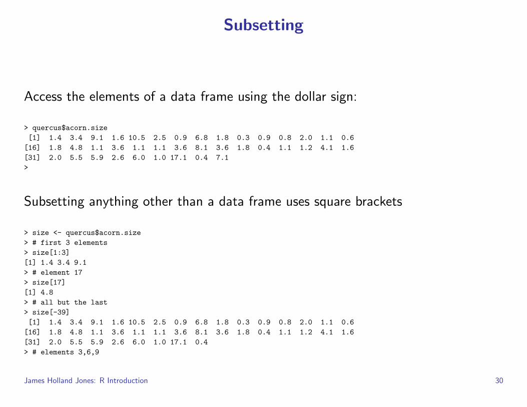
Subsetting
Access the elements of a data frame using the dollar sign:
> quercus$acorn.size[1] 1.4 3.4 9.1 1.6 10.5 2.5 0.9 6.8 1.8 0.3 0.9 0.8 2.0 1.1 0.6[16] 1.8 4.8 1.1 3.6 1.1 1.1 3.6 8.1 3.6 1.8 0.4 1.1 1.2 4.1 1.6[31] 2.0 5.5 5.9 2.6 6.0 1.0 17.1 0.4 7.1>
Subsetting anything other than a data frame uses square brackets
> size <- quercus$acorn.size> # first 3 elements> size[1:3][1] 1.4 3.4 9.1> # element 17> size[17][1] 4.8> # all but the last> size[-39][1] 1.4 3.4 9.1 1.6 10.5 2.5 0.9 6.8 1.8 0.3 0.9 0.8 2.0 1.1 0.6[16] 1.8 4.8 1.1 3.6 1.1 1.1 3.6 8.1 3.6 1.8 0.4 1.1 1.2 4.1 1.6[31] 2.0 5.5 5.9 2.6 6.0 1.0 17.1 0.4> # elements 3,6,9
James Holland Jones: R Introduction 30

> size[c(3,6,9)][1] 9.1 2.5 1.8> # using a logical> # note this uses one of the variables in the data frame "quercus"> # to subset the vector we extracted> size[quercus$Region=="California"][1] 4.1 1.6 2.0 5.5 5.9 2.6 6.0 1.0 17.1 0.4 7.1> # access an element of an array or data frame by X[row,col]> quercus[3,4][1] 9.1# for data frames with named columns, access by col name> quercus[,"tree.height"][1] 27.0 21.0 25.0 3.0 24.0 17.0 15.0 0.3 24.0 11.0 15.0 23.0 24.0 3.0 13.0[16] 30.0 9.0 27.0 9.0 24.0 23.0 27.0 24.0 23.0 18.0 9.0 9.0 4.0 18.0 6.0[31] 17.0 20.0 30.0 23.0 26.0 21.0 15.0 1.0 18.0>
The comma with nothing in front of it means take every row in the the columnnamed "tree.height"
James Holland Jones: R Introduction 31

Subsetting Notes
positive indices include, negative indices exclude elements
1:3 means a sequence from 1 to 3
You can only use a single negative subscript, i.e., you can’t usequercus$acorn.size[-1:3]
Of course, you can get around this by enclosing the vector in parenthesesquercus$acorn.size[-(1:3)]
To test for equality, you need to equals signs ==
When you refer to a variable in a data frame, you must specify the data frame namefollowed a dollar sign and the variable name quercus$acorn.size
James Holland Jones: R Introduction 32

Subsetting with Logicals
Testing for equality is just a special case of a logical test
James Holland Jones: R Introduction 33

Missing Values
NA is a special code for missing data.
NA pretty much means “Don’t Know”
The presence of NAs in your dataset can lead to some surprising consequences whenyou work with it
You can’t test for a NA the way you would test for any other value (i.e., using the== operator) since variable==NA is like asking in English, is the variable equal tosome number I don’t know? How could you know that?!
R therefore provides the function is.na()
James Holland Jones: R Introduction 34

Creating Lists, Vectors, and Matrices
c() concatenates a list of items
• You use this a lot
• It’s a common mistake to forget the c() when putting together a list of numbers, factors,
etc.
• If you do forget it, you will get a syntax error
# a list of numbers> x <- c(1,2,3,4,5)> x[1] 1 2 3 4 5> col <- c("black","red","green")> col[1] "black" "red" "green"> # concatenating 2 lists> x1 <- c(7,8,9)> y <- c(x,x1)> y[1] 1 2 3 4 5 7 8 9> # don’t forget the 6!> y <- c(x,6,x1)> y[1] 1 2 3 4 5 6 7 8 9
James Holland Jones: R Introduction 35

sequences are formed with seq()
> x <- seq(0,10)> x[1] 0 1 2 3 4 5 6 7 8 9 10> # use the optional by= argument to specific the interval between items> x <- seq(0,10,by=2)> x[1] 0 2 4 6 8 10> # use length= to specify a fixed length and let R figure out the interval lengths> x <- seq(0,1,length=23)> x[1] 0.00000000 0.04545455 0.09090909 0.13636364 0.18181818 0.22727273[7] 0.27272727 0.31818182 0.36363636 0.40909091 0.45454545 0.50000000[13] 0.54545455 0.59090909 0.63636364 0.68181818 0.72727273 0.77272727[19] 0.81818182 0.86363636 0.90909091 0.95454545 1.00000000> # this is often useful for plotting functions
Sometimes you want to repeat a value or set of values – this is useful if your settingup a dataset and want to repeat factors
> rep(2,10)[1] 2 2 2 2 2 2 2 2 2 2> rep(c(1,2),10)[1] 1 2 1 2 1 2 1 2 1 2 1 2 1 2 1 2 1 2 1 2> rep(c(1,2),c(10,10))[1] 1 1 1 1 1 1 1 1 1 1 2 2 2 2 2 2 2 2 2 2> rep("R roolz!",3)[1] "R roolz!" "R roolz!" "R roolz!">
James Holland Jones: R Introduction 36

A vector is a list of numbers – it turns out everything in R is represented as a vectorbut that doesn’t affect your life much
Create a vector using one of the techniques we just discussed
A matrix is a rectangular array of numbers – it is a vector of vectors, with thenumbers indexed by row and column
One way to create matrices is to “bind” columns together using the commandcbind() (or rbind)
> cx1980 <- c(7, 13, 8, 13, 5, 35, 9)> cx1988 <- c(9, 11, 15, 8, 9, 38, 0)> C <- cbind(cx1980, cx1988)> C
cx1980 cx1988[1,] 7 9[2,] 13 11[3,] 8 15[4,] 13 8[5,] 5 9[6,] 35 38[7,] 9 0>
What would happen if I instead typed C <- c(cx1980, cx1988) ?
James Holland Jones: R Introduction 37

> C <- c(cx1980, cx1988)> C[1] 7 13 8 13 5 35 9 9 11 15 8 9 38 0>
Not a matrix, but we can make it one...
> C <- matrix(C,nrow=7,ncol=2)> C
[,1] [,2][1,] 7 9[2,] 13 11[3,] 8 15[4,] 13 8[5,] 5 9[6,] 35 38[7,] 9 0>
What happens if we try to bind columns of different lengths
> cx.boesch <- c(18,10,15,30)> C <- cbind(C,cx.boesch)Warning message:number of rows of resultis not a multiple of vector length (arg 2) in: cbind(1, C, cx.boesch)> C
cx.boesch[1,] 7 9 18
James Holland Jones: R Introduction 38

[2,] 13 11 10[3,] 8 15 15[4,] 13 8 30[5,] 5 9 18[6,] 35 38 10[7,] 9 0 15>
Both the warning message and the output can seem a little odd to the uninitiated
> a <- c(2,4)> b <- c(1,3,1,3)> cbind(a,b)
a b[1,] 2 1[2,] 4 3[3,] 2 1[4,] 4 3
R uses a recycling rule for filling out vectors and matrices – when you try to puttogether things that are neither the same length nor multiples of each other, youget a warning
Use the recycling rule to make a matrix of ones
> x <- matrix(1,nr=3,nc=3)> x
James Holland Jones: R Introduction 39

[,1] [,2] [,3][1,] 1 1 1[2,] 1 1 1[3,] 1 1 1>
Note that using the short version of nrow, nr, is sufficient. This is often true – youcan use the minimum name that is unambiguous
James Holland Jones: R Introduction 40

Add-On Packages
One of the great advantages of R is all the user-contributed packages. Frequently,these packages are written by the people who invent the technique!
R version 2.+ uses a graphical package manager for most (all?) platforms – it ispretty self-explanatory
In order to use an R package in a work session, you use the command library()
> library(survival)Loading required package: splines>
Sometimes you will get a message (as you do for survival), sometimes you won’t
You need to load the package every time you start a new R session
Find out from the command line what packages are available:
James Holland Jones: R Introduction 41

> library()Packages in library ’/Library/Frameworks/R.framework/Resources/library’:
AnnBuilder Bioconductor annotation data package builderBiobase Biobase: Base functions for BioconductorBiostrings String objects reepresenting biological
sequencesCategory Category AnalysisChromoViz Multimodal visualization of gene expression
dataCoCiteStats Different test statistics based on co-citation.DEDS Differential Expression via Distance Summary
for Microarray DataDNAcopy DNA copy number data analysisDynDoc Dynamic document toolsEBarrays Empirical Bayes for MicroarraysEpi A package for statistical analysis in
epidemiology.GRASS Interface between GRASS 5.0 geographical
information system and RISwR Introductory Statistics with RKernSmooth Functions for kernel smoothing for Wand & Jones
(1995)MASS Main Package of Venables and Ripley’s MASSUsingR Data sets for the text "Using R for
Introductory Statistics"ade4 Analysis of Environmental Data : Exploratory
and Euclidean methods in Environmental sciences...
James Holland Jones: R Introduction 42

Vectorized Calculation
We frequently want to perform arithmetic operations on lists
This is easy to do in R
A simple model for the annual rate of increase for an iteroparous organism is
λ = s+ b
where s is the average annual survival probability, and b is the average fertility ofeach adult
Given some values of s and b, we can calculate λ
> s <- c(0.9544535, 0.9424282, 0.9416734, 0.9338940, 0.9195420,0.9509079, 0.9561570, 0.9641317, 0.9071128, 0.9448746)
> b <- c(0.044712181, 0.051761901, 0.055269254, 0.009568243,
James Holland Jones: R Introduction 43

0.084174678, 0.037728583, 0.100465837, 0.055931991, 0.068072939,0.015960763)
> lambda <- s+b> lambda[1] 0.9991657 0.9941901 0.9969426 0.9434622 1.0037167 0.9886365 1.0566229[8] 1.0200637 0.9751857 0.9608354
Some funny things can happen with vectorized arithmetic, so beware
What happens here?
> a <- c(1,2,3,4)> b <- c(5,7)> c <- a+b
But if we try this:
> b <- c(5,7,9)> c <- a+bWarning message:longer object lengthis not a multiple of shorter object length in: a + b
This trick results from R’s recycling rule
James Holland Jones: R Introduction 44

A Funky Bit of R Syntax
The value of this function is not likely to be immediately apparent
I will nonetheless present it anyway since I am likely to use it, so you should knowwhat I’m doing
R, like any other computational environment, has scope rules.
Scope describes the range in a program where a variable or function is visible andaccessible
Variable names in data frames are not immediately available to the workspace – youhave to use the data frame name - dollar sign - variable name syntax
Sometimes this can be cumbersome and R allows you to set up a temporary localenvironment that allows you to call variable names without the data frame names
> load("/Users/jhj1/Teaching/a192/datasets/body.size.RData")> with(body.size, plot(height[sex==1],weight[sex==1], xlab="Height (in)", ylab="Weight (lbs)"))
James Holland Jones: R Introduction 45

with() essentially says: use this dataset for everything enclosed in these parentheses
James Holland Jones: R Introduction 46

Bivariate Plots
Do big mammals sleep more than little mammals?
sleep <- read.table("/Users/jhj1/Teaching/a192/datasets/sleep.data.dat",header=TRUE)with(sleep, plot(body,tsleep,log="xy"))
James Holland Jones: R Introduction 47

Nope
●
●
●
●
●
●
●
●
●
●
●
●
●
●
● ●
●●
●
●
●
●
●
●
●●
●
●
●
●
●
●
●●
●●
●
●●
●
●
●●
●●
● ●
●
●
●
●
●●
●
●
●
●
●
1e−02 1e+00 1e+02 1e+04
510
1520
body
tsle
ep
James Holland Jones: R Introduction 48

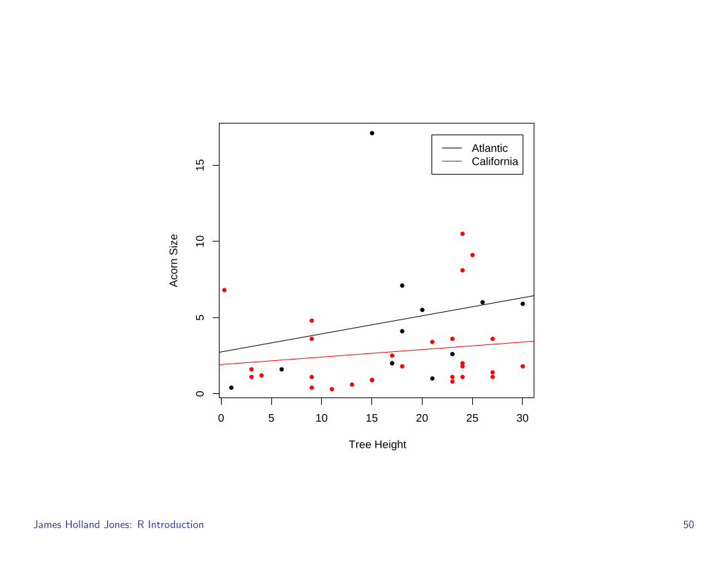
More Bivariate Plots
Here is a pretty complicated plot of Acorn size vs. tree height in two biogeographicallydistinct groups of oaks
This is the sort of plot we would want to construct to evaluate the hypothesis thatrelative acorn size in Californian oaks is smaller than in Atlantic oaks
quercus <- read.delim("/Users/jhj1/Teaching/a192/datasets/quercus.txt", skip=24,sep="�", header=TRUE)
with(quercus, plot(tree.height[Region=="California"],acorn.size[Region=="California"], xlab="Tree Height", pch=20, ylab="Acorn Size"))
with(quercus, points(tree.height[!Region=="California"],acorn.size[!Region=="California"], pch=20, col="red"))
z1 <- with(quercus, lm(acorn.size[Region=="California"] ~tree.height[Region=="California"]))
z2 <- with(quercus, lm(acorn.size[!Region=="California"] ~tree.height[!Region=="California"]))
abline(z1)abline(z2, col="red")
legend(22,17, c("Atlantic","California"), lty=1, col=c("black", "red"))
James Holland Jones: R Introduction 49
●
●
●
●
●
●
●
●
●
●
●
0 5 10 15 20 25 30
05
1015
Tree Height
Aco
rn S
ize
●
●
●
●
●
●
●
●
●
●
● ●
●
●
●
●
●
●
●
●●
●
●
●
●
●
●●
AtlanticCalifornia
James Holland Jones: R Introduction 50

Histograms
Histograms are an excellent way to explore the distributional properties of your data
# simulate 200 standard normal deviatesx1 <- rnorm(200)
# now another 50 with the same mean (0) but high variancex2 <- rnorm(50,0,3)
x <- c(x1,x2)aaa <- max(dnorm(x))
hist(x,50,freq=F,ylim=c(0,aaa), main="")curve(dnorm(x), add=T)
James Holland Jones: R Introduction 51

x
Den
sity
−10 −5 0 5
0.0
0.1
0.2
0.3
0.4
James Holland Jones: R Introduction 52

More On Histograms
Histograms are important enough to consider them in more detail
Consider the Randall-Maciver (1905) dataset of four measurements on 150 Egyptianskulls from 4100 BP to 1755 CE
We will use a histogram to explore a bit
> skulls <- read.table("/Users/jhj1/Teaching/a192/datasets/egyptian-skulls.txt",header=TRUE, skip=25)> summary(skulls)
MB BH BL NHMin. :119.0 Min. :120.0 Min. : 81.00 Min. :44.001st Qu.:131.0 1st Qu.:129.0 1st Qu.: 93.00 1st Qu.:49.00Median :134.0 Median :133.0 Median : 96.00 Median :51.00Mean :134.0 Mean :132.5 Mean : 96.46 Mean :50.933rd Qu.:137.0 3rd Qu.:136.0 3rd Qu.:100.00 3rd Qu.:53.00Max. :148.0 Max. :145.0 Max. :114.00 Max. :60.00
YearMin. :-40001st Qu.:-3300Median :-1850Mean :-18403rd Qu.: -200Max. : 150> hist(skulls$MB)
James Holland Jones: R Introduction 53

While the plot is very helpful, it doesn’t look so great
Histogram of skulls$MB
skulls$MB
Fre
quen
cy
115 120 125 130 135 140 145 150
010
2030
4050
James Holland Jones: R Introduction 54
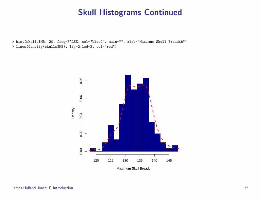
Skull Histograms Continued
> hist(skulls$MB, 20, freq=FALSE, col="blue4", main="", xlab="Maximum Skull Breadth")> lines(density(skulls$MB), lty=2,lwd=3, col="red")
Maximum Skull Breadth
Den
sity
120 125 130 135 140 145
0.00
0.02
0.04
0.06
0.08
James Holland Jones: R Introduction 55

What I Done
What did I do here?
First, I changed the number of bins that the histogram uses with the secondargument (i.e., 20)
Changed it from a frequency histogram to an probability histogram usingfreq=FALSE (Why would I do such a thing?)
Colored the bars with a nice blue, col=blue4
Suppressed the title (main="") and labeled the abscissa with something meaningful(xlab="Maximum Skull Breadth")
Finally, I used a kernel density estimator to draw a non-parametric estimate of theprobability density given by this histogram (this is why I used the freq=FALSEargument)
I used the lines() command, which is a way of adding a line to an existing plot,to add the density estimator
James Holland Jones: R Introduction 56

The argument lty=2 makes the line dashed and the argument lwd=3 made the linewidth 3 pixels (if on a computer screen) or 2.25 points on a pdf graphics device
This density is rather suggestive that we might have a mixture of multiple populationsin this sample because of its pronounced bimodality
James Holland Jones: R Introduction 57

Boxplots
Boxplots give a handy way of exploring the distribution of a sample and of comparingtwo (or more) samples
Creating a boxplot of the contaminated sample and comparing to an uncontaminatedsample gives more weight to the hypothesis that the tails of our contaminated sampleare too heavy
> boxplot(x,y,notch=T,horizontal=T, boxwex=.25)
James Holland Jones: R Introduction 58

● ● ●●●● ●●● ●● ●●
●
−8 −6 −4 −2 0 2 4
James Holland Jones: R Introduction 59

Plotting Expressions
Sometimes you just want to plot a mathematical function
Use expression() to set up a function to plot
expression() basically says here’s something to calculate, but wait until I tell youto do wo with eval()
Calculation are, of course, vectorized
Don’t overdo this one – it has its place, but is rather limited
Plot a normal density the hard way
> nd <- expression((1/sqrt(2*pi*sigma2))*exp(-(x-mu)^2/(2*sigma2)))> x <- seq(-3,3,length=1000)> plot(x,eval(nd), type="l")
In reality, you’d use dnorm() to plot this curve
James Holland Jones: R Introduction 60

−3 −2 −1 0 1 2 3
0.0
0.1
0.2
0.3
0.4
x
eval
(nd)
James Holland Jones: R Introduction 61

Sourcing Code
When you have many commands that you need to execute to perform an analysis orcreate a graphic, it is often convenient to collect those commands into an R script
Call a script using the command source()
Take the example of fitting the logistic model to the USA population series 1790-1930
We need to fit a model with two parameters and do so using nonlinear least-squaresminimization
> usa <- scan("/Users/jhj1/Teaching/summercourse/rdemog/usa.txt")Read 21 items> usa[1] 3.929214 5.308483 7.239881 9.638453 12.866020 17.866020[7] 23.191876 31.443321 38.558371 50.189209 62.979766 76.212168[13] 92.228496 106.021537 123.202624 132.164569 151.325798 179.323175[19] 203.302031 226.542199 248.709873> year <- seq(1790,1990,by=10)> year1 <- year[1:15]> usa1 <- usa[1:15]> logistic.int <- expression(n0 * exp(p[1] * t)/(1 + n0 * (exp(p[1] *t) - 1)/p[2]))
James Holland Jones: R Introduction 62

> r.guess <- (log(usa1[15])-log(usa1[1]))/140> r.guess[1] 0.02460994> k.guess <- usa1[15]> par <- c(r.guess,k.guess)> source("/Users/jhj1/Teaching/summercourse/rdemog/fit.logistic.r")> usa1930.fit <- optim(par,fit.logistic,y=usa1)> usa1930.fit$par[1] 0.03126429 198.61573375
$value[1] 4.830198
$countsfunction gradient
193 NA
$convergence[1] 0
$messageNULL
James Holland Jones: R Introduction 63

Another Example
Say we want to look at the sex-specific scaling of body mass with height
Use data from NHANES
Produce a scatter plot of body mass vs. stature
Fit smooth curves for males and females separately
Here is a script to produce the plot – enter and save this using a text editor:
# Plots body mass (kg) against stature (cm) for 18,648 complete# observations from the NHANES data# draws Friedman’s super smoother curves for males and females
# data already extracted from NHANES and saved as a binary fileload("body.size.RData")
# get rid of NAs so supsmu doesn’t shoot out warningscheight <- !is.na(body.size$height)cweight <- !is.na(body.size$weight)height <- body.size$height[cheight & cweight]weight <- body.size$weight[cheight & cweight]
James Holland Jones: R Introduction 64

sex <- body.size$sex[cheight & cweight]
# convert to metric!plot(height*2.54,weight/2.2, pch=".", xlab="Height (cm)", ylab="Weight (kg)")lines(supsmu(2.54*height[sex==1],weight[sex==1]/2.2),lwd=2)lines(supsmu(2.54*height[sex==2],weight[sex==2]/2.2),lwd=2, col="red")legend(200,200, c("Men", "Women"), lwd=2, col=c("black", "red"))title("Sex-Specific Scaling of Body Mass with Height")
Now source the code
> source("make.demo.plot.r")
James Holland Jones: R Introduction 65

120 140 160 180 200 220
5010
015
020
0
Height (cm)
Wei
ght (
kg)
MenWomen
Sex−Specific Scaling of Body Mass with Height
James Holland Jones: R Introduction 66
Recommended


![A hybrid smoothed dissipative particle dynamics (SDPD ...the deterministic spatial dynamics but not the stochastic dynamics. The spatial stochastic simulation 80 algorithm (sSSA) [29]](https://img.dokumen.tips/doc/110x75/5f41a2ab66492703c57addfe/a-hybrid-smoothed-dissipative-particle-dynamics-sdpd-the-deterministic-spatial.jpg)


