Stefanos Zafeiriou Adv. Statistical Machine Learning(495)
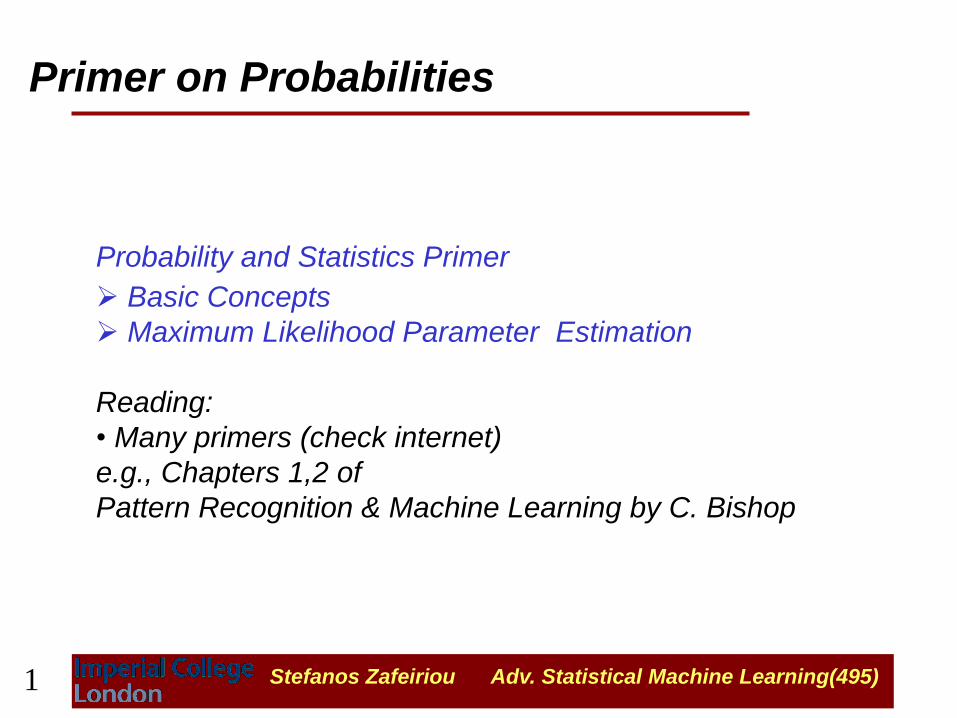
Primer on Probabilities
Probability and Statistics Primer
Basic Concepts
Maximum Likelihood Parameter Estimation
Reading:
• Many primers (check internet)
e.g., Chapters 1,2 of
Pattern Recognition & Machine Learning by C. Bishop
1
Stefanos Zafeiriou Adv. Statistical Machine Learning(495)
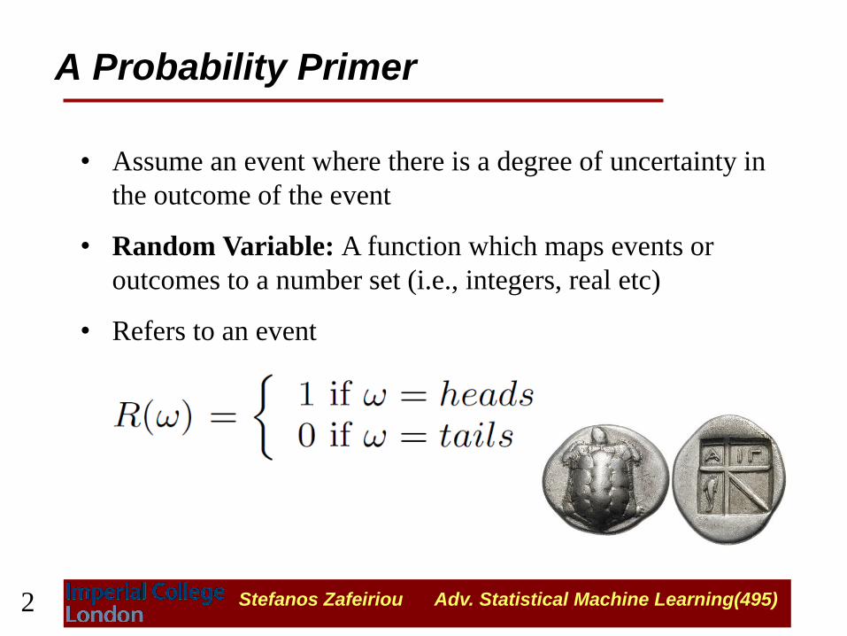
A Probability Primer
• Assume an event where there is a degree of uncertainty in
the outcome of the event
• Random Variable: A function which maps events or
outcomes to a number set (i.e., integers, real etc)
• Refers to an event
2

Stefanos Zafeiriou Adv. Statistical Machine Learning(495)
Frequentistic Definition
• Frequency Probability:
Probability is the limit of its relative frequency in
a large number of trials
or approx.
• It is the relative frequency with which an outcome would
be obtained if the process were repeated a large number of
times under exactly the same conditions.
𝑝(𝑥)
𝑝(𝑥)= lim𝑛→∞
𝑛𝑥
𝑛𝑡 𝑝(𝑥)≈
𝑛𝑥
𝑛𝑡
3
Stefanos Zafeiriou Adv. Statistical Machine Learning(495)
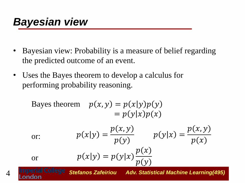
• Bayesian view: Probability is a measure of belief regarding
the predicted outcome of an event.
• Uses the Bayes theorem to develop a calculus for
performing probability reasoning.
Bayesian view
Bayes theorem
or:
or
𝑝 𝑥, 𝑦 = 𝑝 𝑥 𝑦 𝑝 𝑦
= 𝑝 𝑦 𝑥 𝑝(𝑥)
𝑝 𝑥 𝑦 =𝑝(𝑥, 𝑦)
𝑝(𝑦) 𝑝 𝑦 𝑥 =
𝑝(𝑥, 𝑦)
𝑝(𝑥)
𝑝 𝑥 𝑦 = 𝑝(𝑦|𝑥)𝑝(𝑥)
𝑝(𝑦)
4

Stefanos Zafeiriou Adv. Statistical Machine Learning(495)
Joint Probability Distribution
• Joint probabilities can be between
any number of variables
eg.
• For every combination of variables
we need to define how probable
that combination is
• The probabilities of all
combinations need to sum up to 1.
• For 3 random variables taking two
values the table contains 8 entries
𝑎 𝑏 𝑐
0 0 0 0.1
0 0 1 0.2
0 1 0 0.05
0 1 1 0.05
1 0 0 0.3
1 0 1 0.1
1 1 0 0.05
1 1 1 0.15
Sum up to
1
𝑝(𝑎 = 1, 𝑏 = 1, 𝑐 = 1)
𝑝(𝑎, 𝑏, 𝑐)
5

Stefanos Zafeiriou Adv. Statistical Machine Learning(495)
Joint Probability Distribution
• Given the joint probability distribution, you can calculate any probability involving 𝑎, 𝑏, and 𝑐
• Note: May need to use marginalization and Bayes rule, (both of which are not discussed in these slides)
𝑎 𝑏 𝑐
0 0 0 0.1
0 0 1 0.2
0 1 0 0.05
0 1 1 0.05
1 0 0 0.3
1 0 1 0.1
1 1 0 0.05
1 1 1 0.15 Examples of things you can compute:
•
•
𝑝(𝑎, 𝑏, 𝑐)
𝑝 𝑎 = 1 = 𝑝 𝑎 = 1, 𝑏, 𝑐 𝑠𝑢𝑚 𝑟𝑜𝑤𝑠 𝑎 = 1
𝑏,𝑐
𝑝 𝑎 = 1, 𝑏 = 1|𝑐 = 1 =
𝑝 𝑎 = 1, 𝑏 = 1, 𝑐 = 1 |𝑝 𝑐 = 1 (𝐵𝑎𝑦𝑒𝑠 𝑇ℎ𝑒𝑜𝑟𝑒𝑚)
6
Stefanos Zafeiriou Adv. Statistical Machine Learning(495)
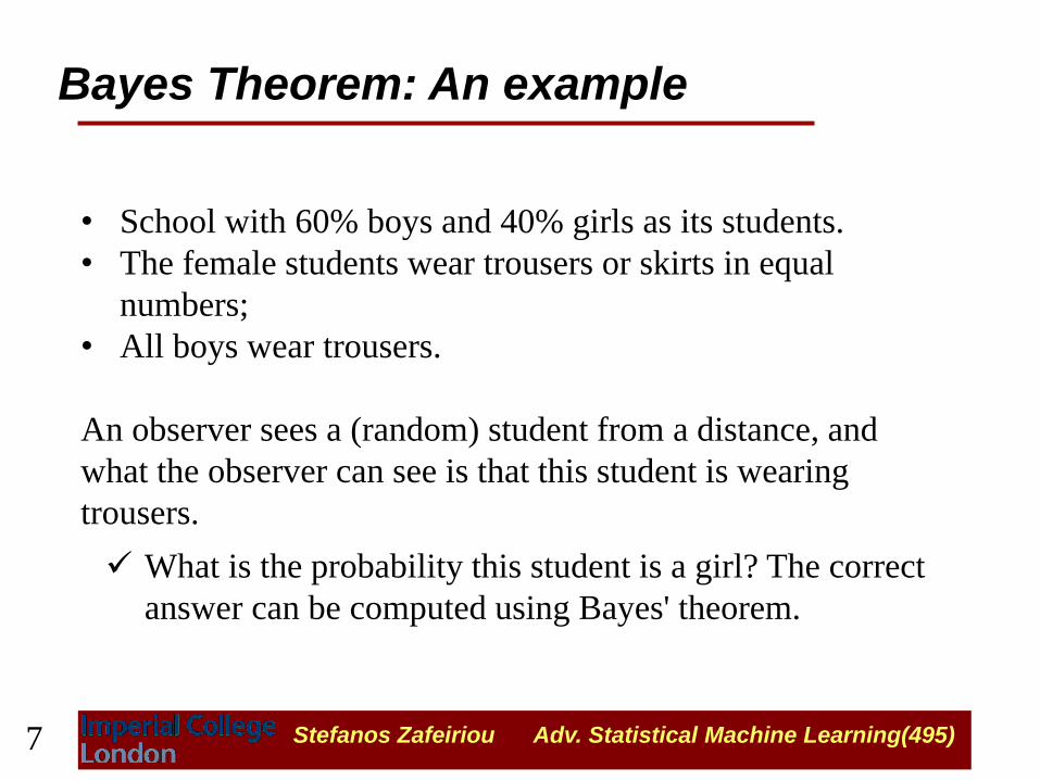
Bayes Theorem: An example
• School with 60% boys and 40% girls as its students.
• The female students wear trousers or skirts in equal
numbers;
• All boys wear trousers.
An observer sees a (random) student from a distance, and
what the observer can see is that this student is wearing
trousers.
What is the probability this student is a girl? The correct
answer can be computed using Bayes' theorem.
7

Stefanos Zafeiriou Adv. Statistical Machine Learning(495)
Bayes Theorem: An example
8

Stefanos Zafeiriou Adv. Statistical Machine Learning(495)
The requested probability is translated as:
An observer sees a (random)
student from a distance, and what
the observer can see is that this
student is wearing trousers.
• What is the probability this
student is a girl?
Bayes Theorem: An example
9

Stefanos Zafeiriou Adv. Statistical Machine Learning(495)
• Bayes theorem:
• What do we
know?
• What are we missing?
Bayes Theorem: An example
10
Stefanos Zafeiriou Adv. Statistical Machine Learning(495)
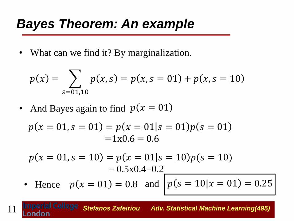
• What can we find it? By marginalization.
• And Bayes again to find
Bayes Theorem: An example
• Hence and
𝑝 𝑥 = 01, 𝑠 = 10 = 𝑝 𝑥 = 01 𝑠 = 10 𝑝(𝑠 = 10) = 0.5x0.4=0.2
𝑝 𝑥 = 01
11

Stefanos Zafeiriou Adv. Statistical Machine Learning(495)
Independence
How is independence useful?
• Suppose you have n coin flips and you want to
calculate the joint distribution p(c1, …, cn)
• If the coin flips are not independent, you need 2n
values in the table
• If the coin flips are independent, then
n
i
in cpccp1
1 )(),...,( Each p(ci) table has 2 entries and
there are n of them for a total of
2n values
12

Stefanos Zafeiriou Adv. Statistical Machine Learning(495)
Independence
Variables a and b are conditionally
independent given c if any of the following
hold:
• p(a,b|c) = p(a|c) p(b|c)
• p(a|b,c)= p(a|c)
• p(b|a,c) = p(b|c)
Knowing c tells me everything about b (ie. I don’t gain
anything by knowing a). Either because a doesn’t
influence b or because knowing c provides all the
information knowing a would give.
𝑐
𝑎 𝑏
13
Stefanos Zafeiriou Adv. Statistical Machine Learning(495)
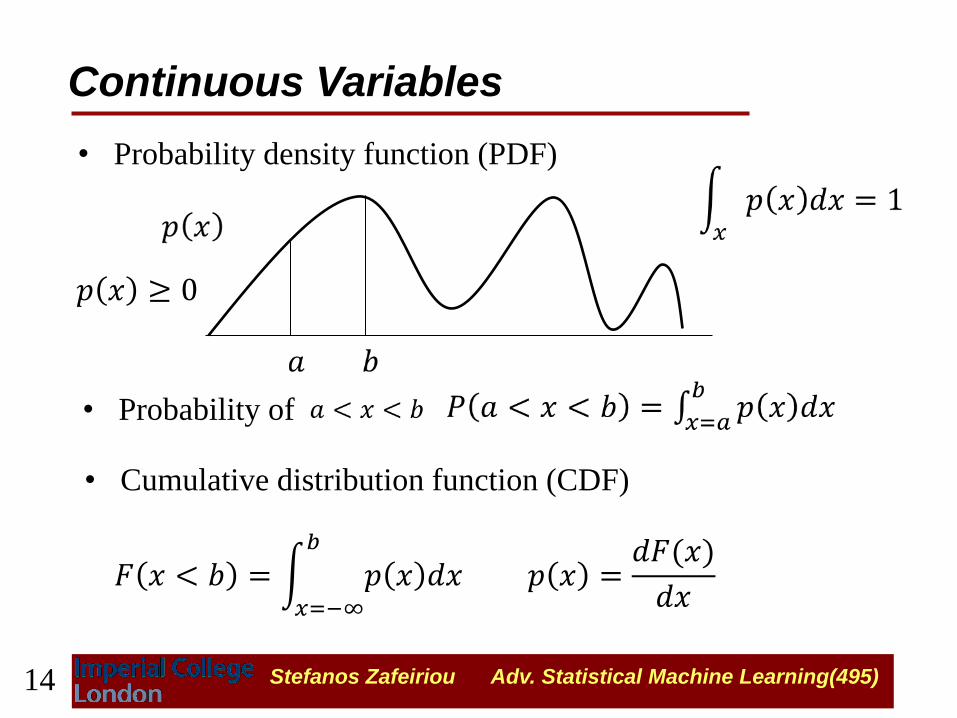
Continuous Variables
• Probability density function (PDF)
• Probability of
• Cumulative distribution function (CDF)
𝐹 𝑥 < 𝑏 = 𝑝 𝑥 𝑑𝑥𝑏
𝑥=−∞
𝑝 𝑥 =𝑑𝐹(𝑥)
𝑑𝑥
𝑝 𝑥 ≥ 0
14
Stefanos Zafeiriou Adv. Statistical Machine Learning(495)
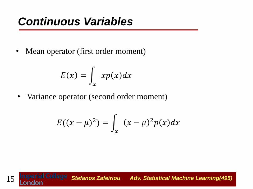
• Mean operator (first order moment)
Continuous Variables
• Variance operator (second order moment)
𝐸 𝑥 = 𝑥𝑝 𝑥 𝑑𝑥𝑥
𝐸((𝑥 − 𝜇)2) = 𝑥 − 𝜇 2𝑝 𝑥 𝑑𝑥𝑥
15

Stefanos Zafeiriou Adv. Statistical Machine Learning(495)
Popular PDFs
• Gaussian or Normal distribution
• CDF
• Parameters the mean and
standard deviations
𝑝 𝑥 =1
𝜎 2𝜋𝑒−12𝜎2(𝑥−𝜇)2
𝜇, 𝜎2
𝑥~𝑁(𝑥|𝜇, 𝜎2)
𝐸 𝑥 = 𝜇 𝐸 𝑥 − 𝜇 2 = 𝜎2
16

Stefanos Zafeiriou Adv. Statistical Machine Learning(495)
Parameter estimation with Gaussians
• What is estimation? Given a set of observations and a
model - estimate the model’s parameter.
• First example: Given a population
assuming that are independent samples from a normal
distribution find an estimate for
• How we approach the problem?
(1) We write the joint probability distribution (likelihood).
{𝑥1, 𝑥2, 𝑥3,…𝑥𝑁}
𝑥~𝑁(𝑥|𝜇, 𝜎2) 𝜇, 𝜎2
𝑝(𝑥1, 𝑥2, 𝑥3,…𝑥𝑁|𝜇, 𝜎2)= 𝑝(𝑥𝑖|𝜇, 𝜎
2)𝑁𝑖=1
17

Stefanos Zafeiriou Adv. Statistical Machine Learning(495)
(2) We substitute our distributional assumptions.
(3) A common practice is to take the log of the joint function
Parameter estimation with Gaussians
𝑝(𝑥1, 𝑥2, 𝑥3,…𝑥𝑁|𝜇, 𝜎2)=
1
𝜎 2𝜋𝑒− 𝑥𝑖−𝜇
2/𝜎2𝑁𝑖=1
=(2𝜋)−𝑁/2
𝜎𝑁𝑒− (𝑥𝑖−𝜇)
2/2𝜎2𝑁𝑖=1
log 𝑝 𝜇, 𝜎2 = −1
2Nlog2π − Nlog 𝜎 −
(𝑥𝑖 − 𝜇)2𝑁
𝑖=1
2𝜎2
18
Stefanos Zafeiriou Adv. Statistical Machine Learning(495)
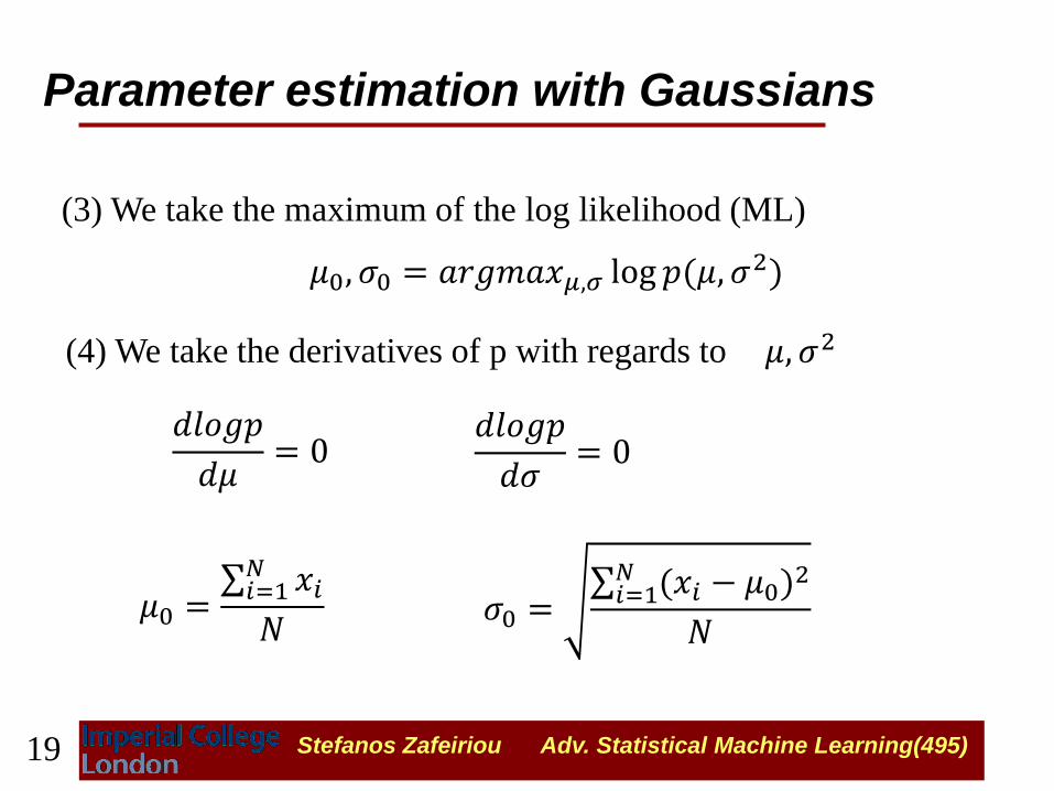
(3) We take the maximum of the log likelihood (ML)
Parameter estimation with Gaussians
(4) We take the derivatives of p with regards to
𝜇0, 𝜎0 = 𝑎𝑟𝑔𝑚𝑎𝑥𝜇,𝜎 log 𝑝(𝜇, 𝜎2)
𝜇, 𝜎2
𝑑𝑙𝑜𝑔𝑝
𝑑𝜇= 0
𝑑𝑙𝑜𝑔𝑝
𝑑𝜎= 0
𝜇0 = 𝑥𝑖𝑁𝑖=1
𝑁 𝜎0 =
(𝑥𝑖 − 𝜇0)2𝑁
𝑖=1
𝑁
19
Stefanos Zafeiriou Adv. Statistical Machine Learning(495)
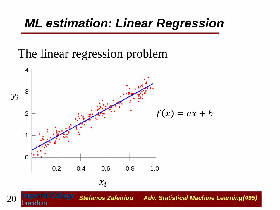
The linear regression problem
ML estimation: Linear Regression
𝑓 𝑥 = 𝑎𝑥 + 𝑏
𝑦𝑖
𝑥𝑖
20
Stefanos Zafeiriou Adv. Statistical Machine Learning(495)
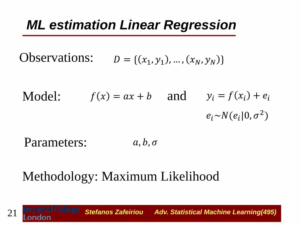
Observations:
ML estimation Linear Regression
Model: and
Parameters:
Methodology: Maximum Likelihood
𝐷 = { 𝑥1, 𝑦1 , … , 𝑥𝑁, 𝑦𝑁 }
𝑦𝑖 = 𝑓 𝑥𝑖 + 𝑒𝑖 𝑓 𝑥 = 𝑎𝑥 + 𝑏
𝑒𝑖~𝑁(𝑒𝑖|0, 𝜎2)
𝑎, 𝑏, 𝜎
21

Stefanos Zafeiriou Adv. Statistical Machine Learning(495)
(1) We write the joint probability distribution (likelihood).
𝑝((𝑥1, 𝑦1), (𝑥2, 𝑦2),…, (𝑥𝑁, 𝑦𝑁)|𝑓, 𝜎2)
= 𝑝 (𝑥𝑖 , 𝑦𝑖 |𝑓, 𝜎2)𝑁
𝑖=1
= 𝑝 𝑦𝑖 𝑓, 𝜎2, 𝑥𝑖 𝑝(𝑥𝑖)
𝑁𝑖=1
𝑁𝑖=1
we need to compute the following probability 𝑝 𝑦𝑖 𝑓, 𝜎2, 𝑥𝑖
ML estimation Linear Regression
𝑦𝑖 = 𝑓 𝑥𝑖 + 𝑒𝑖 we know that
𝑒𝑖~𝑁(𝑒𝑖|0, 𝜎2)
22

Stefanos Zafeiriou Adv. Statistical Machine Learning(495)
Assume a random variable with pdf
• Change of random variables
ML estimation Linear Regression
𝑎 𝑝𝑎
Assume a second random variable and that are
related by
𝑏 𝑎, 𝑏 𝑏 = 𝑔(𝑎)
What is the pdf of ? 𝑏 𝑝𝑏
| 𝑝𝑏 𝑏 𝑑𝑏| = |𝑝𝑎 𝑎 𝑑𝑎|
𝑝𝑏 𝑏 = |𝑑𝑎
𝑑𝑏|𝑝𝑎 𝑎
𝑝𝑏 𝑏 = |𝑑𝑔−1(𝑏)
𝑑𝑏|𝑝𝑎 𝑔
−1(𝑏)
23

Stefanos Zafeiriou Adv. Statistical Machine Learning(495)
• Lets go back to our case
ML estimation Linear Regression
𝑝(𝑒𝑖) = 𝑁(𝑒𝑖|0, 𝜎2) 𝑦𝑖 = 𝑔 𝑒𝑖 = 𝑓 𝑥𝑖 + 𝑒𝑖
we compute using the previous 𝑝(𝑦𝑖)
𝑝(𝑦𝑖) = 𝑁(𝑦𝑖 − 𝑓(𝑥𝑖)|0, 𝜎2)
𝑒𝑖 = 𝑦𝑖 − 𝑓(𝑥𝑖)
𝑝(𝑦𝑖 𝑥𝑖 , 𝑓, 𝜎2 = 𝑁 𝑦𝑖|𝑓(𝑥𝑖 , 𝜎
2)
or putting back what is constant we write more correctly
24
Stefanos Zafeiriou Adv. Statistical Machine Learning(495)
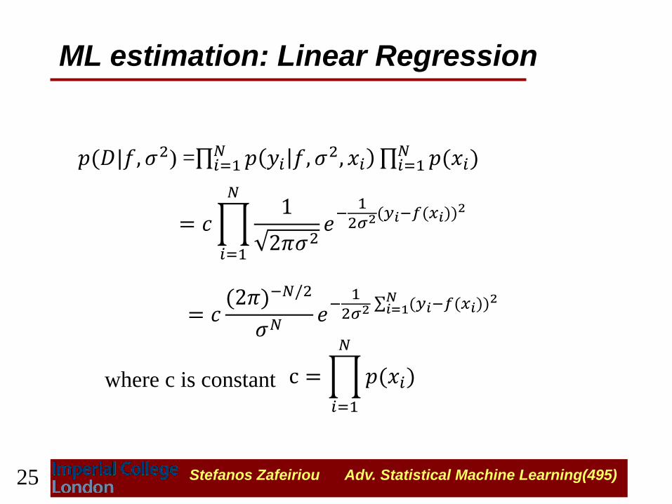
𝑝(𝐷|𝑓, 𝜎2) = 𝑝 𝑦𝑖 𝑓, 𝜎2, 𝑥𝑖 𝑝(𝑥𝑖)
𝑁𝑖=1
𝑁𝑖=1
= 𝑐 1
2𝜋𝜎2𝑒−12𝜎2(𝑦𝑖−𝑓(𝑥𝑖))
2
𝑁
𝑖=1
where c is constant c = 𝑝(𝑥𝑖)
𝑁
𝑖=1
= 𝑐(2𝜋)−𝑁/2
𝜎𝑁𝑒−12𝜎2 (𝑦𝑖−𝑓(𝑥𝑖))
2𝑁𝑖=1
ML estimation: Linear Regression
25
Stefanos Zafeiriou Adv. Statistical Machine Learning(495)
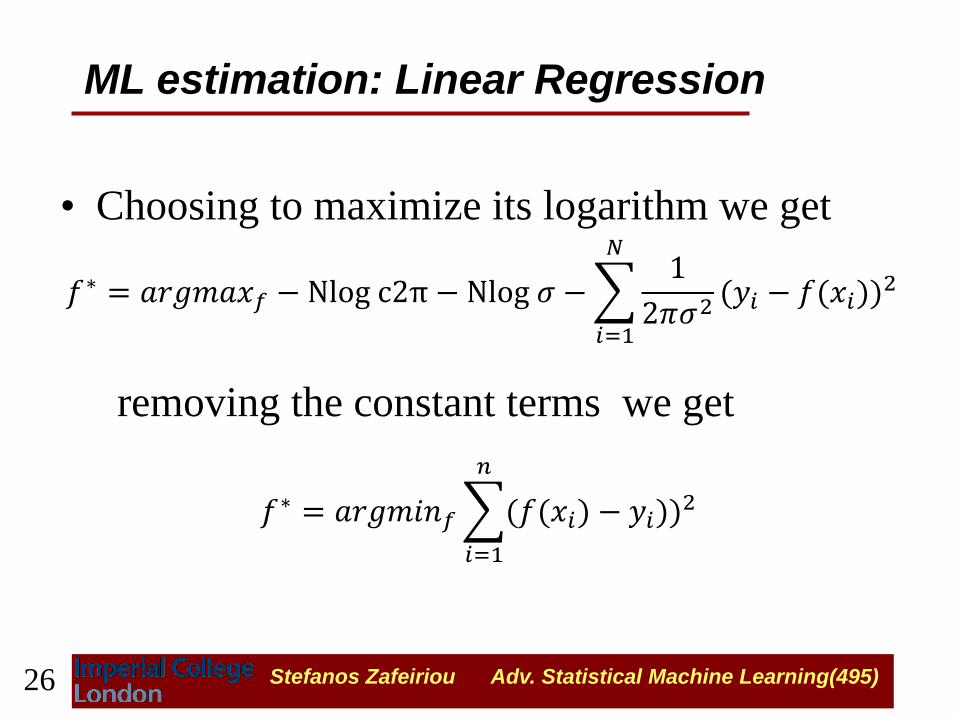
• Choosing to maximize its logarithm we get
removing the constant terms we get
𝑓∗ = 𝑎𝑟𝑔𝑚𝑎𝑥𝑓 − Nlog c2π − Nlog 𝜎 − 1
2𝜋𝜎2(𝑦𝑖 − 𝑓(𝑥𝑖))
2
𝑁
𝑖=1
𝑓∗ = 𝑎𝑟𝑔𝑚𝑖𝑛𝑓 (𝑓(𝑥𝑖) − 𝑦𝑖))2
𝑛
𝑖=1
ML estimation: Linear Regression
26

Stefanos Zafeiriou Adv. Statistical Machine Learning(495)
by taking the partial derivative with respect to a and b and setting
them equal to zero we get
𝑓∗ = 𝑎𝑟𝑔𝑚𝑖𝑛𝑓 (𝑎𝑥𝑖 + 𝑏 − 𝑦𝑖)2
𝑁
𝑖=1
𝑔 𝑎, 𝑏 = (𝑎𝑥𝑖 + 𝑏 − 𝑦𝑖)2
𝑁
𝑖=1
𝜕𝑔
𝜕𝑏= 0 → 2 𝑎𝑥𝑖 + 𝑏 − 𝑦𝑖 = 0 → 𝑁𝑏 = − 𝑎𝑥𝑖 + 𝑦𝑖 →
𝑁
𝑖=1
𝑁
𝑖=1
𝑁
𝑖=1
𝑏 = 𝑦 − 𝑎𝑥 1 𝑦 =1
𝑁 𝑦𝑖
𝑁
𝑖=1
𝑎𝑛𝑑 𝑥 =1
𝑁 𝑥𝑖
𝑁
𝑖=1
ML estimation: Linear Regression
27
Stefanos Zafeiriou Adv. Statistical Machine Learning(495)
putting (1) into (2) we get
𝑥𝑖𝑦𝑖 −𝑁𝑥 𝑦 = 𝑎
𝑁
𝑖=1
𝑥𝑖2 − 𝑎𝑁 𝑥 2
𝑁
𝑖=1
→ 𝑎 = 𝑥𝑖𝑦𝑖 −𝑁𝑥 𝑦 𝑁𝑖=1
𝑥𝑖2 −𝑁𝑥 2𝑁
𝑖=1
𝜕𝑔
𝜕𝑎= 0 → 𝑥𝑖 𝑎𝑥𝑖 + 𝑏 − 𝑦𝑖 = 0
𝑁
𝑖=1
→ 𝑥𝑖𝑦𝑖 = 𝑎 𝑥𝑖2 + 𝑏 𝑥𝑖
𝑁
𝑖=1
𝑁
𝑖=1
𝑁
𝑖=1
(2)
ML estimation: Linear Regression
28
Recommended