
Price Dynamics & Trading Strategies in theCommodities Market
Kevin Louis Guo
Submitted in partial fulfillment of the
requirements for the degree
of Doctor of Philosophy
in the Graduate School of Arts and Sciences
Columbia Univeristy
2018

c©2018Kevin Louis Guo
All Rights Reserved
ABSTRACT
Price Dynamics & Trading Strategies in the
Commodities Market
Kevin Louis Guo
This thesis makes new observations of market phenomena for various commodities and
trading strategies centered around these observations. In particular, our results imply that
many aspects of the commodities markets, from delivery markets to producers and consumer
derivative based ETFs can be modeled effectively using financial engineering techniques.
Chapter 2 examines what drives the returns of gold miner stocks and ETFs. Inspired by
our real options model, we construct a method to dynamically replicate gold miner stocks
using two factors: a spot gold ETF and a market equity portfolio. We find that our real
options approach can explain a significant portion of the drivers of firm implied gold leverage.
Chapter 3 studies commodity exchange-traded funds (ETFs). From empirical data, we
find that many commodity leveraged ETFs underperform significantly against our con-
structed dynamic benchmark, and we quantify such a discrepancy via the novel idea of
realized effective fee. Finally, we consider a number of trading strategies and examine their
performance by backtesting with historical price data.
Chapter 4 studies the phenomenon of non-convergence between futures and spot prices
in the grains market. In our proposed approach, we incorporate stochastic spot price and
storage cost, and solve an optimal double stopping problem to understand shipping certificate
prices. Our new models for stochastic storage rates explain the spot-futures premium.
Contents
List of Figures iii
List of Tables v
Acknowledgements vi
1 Introduction 1
2 How to Mine Gold Without Digging 4
2.1 Introduction . . . . . . . . . . . . . . . . . . . . . . . . . . . . . . . . . . . . 4
2.2 Related Studies . . . . . . . . . . . . . . . . . . . . . . . . . . . . . . . . . . 7
2.3 Model . . . . . . . . . . . . . . . . . . . . . . . . . . . . . . . . . . . . . . . 10
2.3.1 Asset Valuation . . . . . . . . . . . . . . . . . . . . . . . . . . . . . . 10
2.3.2 Equity Valuation . . . . . . . . . . . . . . . . . . . . . . . . . . . . . 14
2.3.3 Comparative Statics . . . . . . . . . . . . . . . . . . . . . . . . . . . 18
2.4 Factor Replication of Gold Miner Stocks . . . . . . . . . . . . . . . . . . . . 25
2.4.1 Data . . . . . . . . . . . . . . . . . . . . . . . . . . . . . . . . . . . . 25
2.4.2 Constructing the Replicating Portfolio . . . . . . . . . . . . . . . . . 26
2.5 Estimating Model Parameters with Kalman Filter . . . . . . . . . . . . . . . 31
2.6 Testing Predictions for Gold Miners’ Implied Leverage . . . . . . . . . . . . 36
2.7 Conclusion . . . . . . . . . . . . . . . . . . . . . . . . . . . . . . . . . . . . . 39
i
3 Understanding the Returns of Commodity LETFs 41
3.1 Introduction . . . . . . . . . . . . . . . . . . . . . . . . . . . . . . . . . . . . 42
3.2 Analysis of Tracking Error . . . . . . . . . . . . . . . . . . . . . . . . . . . . 46
3.2.1 Regression of Empirical Returns . . . . . . . . . . . . . . . . . . . . . 46
3.2.2 Distribution of Tracking Errors . . . . . . . . . . . . . . . . . . . . . 48
3.3 Incorporating Realized Variance into Tracking Error Measurement . . . . . . 55
3.3.1 Model for the LETF Price . . . . . . . . . . . . . . . . . . . . . . . . 55
3.3.2 Regression of Empirical Returns . . . . . . . . . . . . . . . . . . . . . 57
3.3.3 Realized Effective Fee . . . . . . . . . . . . . . . . . . . . . . . . . . 59
3.4 A Static LETF Portfolio . . . . . . . . . . . . . . . . . . . . . . . . . . . . . 62
3.5 Concluding Remarks . . . . . . . . . . . . . . . . . . . . . . . . . . . . . . . 68
4 Non-convergence of Agricultural Futures 71
4.1 Introduction . . . . . . . . . . . . . . . . . . . . . . . . . . . . . . . . . . . . 71
4.2 Related Studies . . . . . . . . . . . . . . . . . . . . . . . . . . . . . . . . . . 76
4.3 Martingale Model with Stochastic Storage . . . . . . . . . . . . . . . . . . . 78
4.4 Local Stochastic Storage Model . . . . . . . . . . . . . . . . . . . . . . . . . 93
4.5 Concluding Remarks . . . . . . . . . . . . . . . . . . . . . . . . . . . . . . . 105
4.6 Appendix . . . . . . . . . . . . . . . . . . . . . . . . . . . . . . . . . . . . . 107
4.6.1 Proofs: Proposition 5 . . . . . . . . . . . . . . . . . . . . . . . . . . . 107
4.6.2 Proofs: Proposition 6 . . . . . . . . . . . . . . . . . . . . . . . . . . . 110
References 112
ii
List of Figures
1 Value function of the gold mine vs gold spot price . . . . . . . . . . . . . . . 18
2 Implied leverage as a function of model parameters . . . . . . . . . . . . . . 20
3 Replicating portfolio vs actual gold miner stock performance . . . . . . . . . 29
4 Raw implied leverage vs Kalman Filter implied leverage . . . . . . . . . . . . 35
5 Relationship of implied leverage and gold prices . . . . . . . . . . . . . . . . 37
6 Regression of DJUSEN-DIG Returns . . . . . . . . . . . . . . . . . . . . . . 49
7 Regression of DJUSEN-DUG Returns . . . . . . . . . . . . . . . . . . . . . . 49
8 Regression of GOLDLNPM-UGL Returns . . . . . . . . . . . . . . . . . . . 50
9 Regression of GOLDLNPM-GLL Returns . . . . . . . . . . . . . . . . . . . . 50
10 Estimated β over horizon . . . . . . . . . . . . . . . . . . . . . . . . . . . . . 51
11 Histograms and QQ plots of 1-day tracking errors for DIG, DUG, UGL, GLL 52
12 Mean Tracking Error by Commodity . . . . . . . . . . . . . . . . . . . . . . 54
13 Performance of LETF vs Tracking Portfolio Over Time . . . . . . . . . . . . 60
14 Trading returns vs realized variance for a double short strategy . . . . . . . 66
15 Returns of reference index vs trading returns for a double short strategy . . 67
16 Average returns from a double short trading strategy by commodity pair over
no. of days holding period . . . . . . . . . . . . . . . . . . . . . . . . . . . . 68
17 Time series of returns for a double short strategy over 30-day rolling, holding
periods . . . . . . . . . . . . . . . . . . . . . . . . . . . . . . . . . . . . . . . 69
iii

18 Time series of basis for soybeans and corn futures . . . . . . . . . . . . . . . 73
19 The shipping certificate price as a function of spot price and market storage
rate . . . . . . . . . . . . . . . . . . . . . . . . . . . . . . . . . . . . . . . . 83
20 Calibration of the Martingale Model to empirical corn futures prices . . . . . 90
21 Calibraton of the Martingale Model to empirical wheat futures prices . . . . 91
22 Optimal stopping levels for XOU Model . . . . . . . . . . . . . . . . . . . . 97
23 Certificate Price vs Liquidation and Exercise Value . . . . . . . . . . . . . . 97
24 Calibration of the XOU Model to the empirical corn futures prices . . . . . . 103
25 Calibration of XOU model with local storage to the empirical wheat futures
curve . . . . . . . . . . . . . . . . . . . . . . . . . . . . . . . . . . . . . . . . 103
26 Calibration of the Martingale Model and the XOU Model to the empirical
soybeans futures curve . . . . . . . . . . . . . . . . . . . . . . . . . . . . . . 104
27 Seasonality of the average basis for corn, soybeans, and wheat during 2004–2010105
iv

List of Tables
1 Summary of stock and ETF data used for our analysis . . . . . . . . . . . . 25
2 Replicating portfolio vs actual gold miner stock performance . . . . . . . . . 28
3 Regression: performance of real options model . . . . . . . . . . . . . . . . . 38
4 Data summary of LETFs by commodity type and leverage . . . . . . . . . . 45
5 Mean and STD of tracking error by commodity . . . . . . . . . . . . . . . . 51
6 Volatility Decay Coefficient Table . . . . . . . . . . . . . . . . . . . . . . . . 58
7 Effective fees for LETFs . . . . . . . . . . . . . . . . . . . . . . . . . . . . . 61
8 Weight pairs to execute market-neutral trading strategy . . . . . . . . . . . . 64
9 Basis summary during 2004-2014 before (pre) and after (post) CBOT intro-
duced new certificate policies to facilitate convergence . . . . . . . . . . . . . 92
v

Acknowledgements
In terms of my greatest intellectual inspiration and personal motivator, I would like to
acknowledge Ayn Rand’s magnum opus Atlas Shrugged (see Rand (1957)). It taught me the
importance of money, the virtue of self-interest, and the thrill of creating new knowledge:
Money is the material shape of the principle that men who wish to deal with one
another must deal by trade and give value for value. Money is not the tool of
the moochers, who claim your product by tears, or of the looters, who take it
from you by force. Money is made possible only by the men who produce ... Run
for your life from any man who tells you that money is evil. That sentence is
the leper’s bell of an approaching looter. So long as men live together on earth
and need means to deal with one another-their only substitute, if they abandon
money, is the muzzle of a gun.
Most importantly, this defense couldn’t have taken place without the hard work of my
thesis committee: Garud Iyengar, Dylan Possamai, Miquel Alonso, David Yao, and my
adviser Tim Leung. I especially wish to thank my adviser, who stuck with me all the way back
when I was a junior in undergrad at Columbia. He always knows to which journal to submit,
which research paths to pursue, and which parts of my writing to emphasize. Without his
guidance, I’m certain I would have taken 3 additional years to graduate. Finally, I would
like to acknowledge myself as well. I probably couldn’t have written this thesis without me.
vi

Chapter 1
Introduction
This thesis makes new observations of market phenomena for various commodities and trad-
ing strategies centered around these observations. Unlike equities, commodities cannot be
easily modeled as claims to future cash flows. However, a pure supply-demand model for
commodities as used in elementary economics courses also remains unsatisfactory because
it cannot capture the rich set of incentives which drive the behavior of financial interme-
diaries, producers, and investors. Thus, we turn to the financial engineering literature to
explain these market observations through micro-founded rational agent models. In partic-
ular, we study gold miners as agent optimized claims on future gold production; we show
that non-convergence in grain markets can be explained by the CBOT delivery mechanisms
which have hidden, embedded storage options; and finally, we demonstrate how commodity
leveraged ETFs behave like a dynamic replicating portfolio of their underlying commodities.
In all three chapters, we make heavy use of options pricing, optimal stopping, and optimal
control techniques to understand the underlying dynamics of commodity markets.
Chapter 2 examines what drives the returns of gold miner stocks and ETFs by modeling
them as real options on gold. We solve a double optimal control problem to determine the
best production strategy and the value of the firm equity, demonstrating that gold miner
equities behave like “real options on gold.” Inspired by our real options model, we construct
1
CHAPTER 1. INTRODUCTION 2
a method to dynamically replicate gold miner stocks using two factors: a spot gold ETF and
a market equity portfolio. Furthermore, through each firm’s factor loadings on replicating
portfolio, we can infer the implicit firm leverage parameters of our model using the Kalman
Filter. We find that our real options approach can explain a significant portion of the
drivers of firm implied gold leverage. We posit that gold miner companies hold additional
real options which help mitigate firm volatility, but these real options cause lower returns
relative to the replicating portfolio.
Chapter 3 studies commodity exchange-traded funds (ETFs), which can be modeled as a
dynamic replicating portfolio of an underlying index. In this chapter, we analyze the track-
ing performance of commodity leveraged ETFs and discuss the associated trading strategies.
It is known that leveraged ETF returns typically deviate from their tracking target over
longer holding horizons due to the so-called volatility decay. This motivates us to construct
a benchmark process that accounts for the volatility decay, and use it to examine the tracking
performance of commodity leveraged ETFs. From empirical data, we find that many com-
modity leveraged ETFs underperform significantly against the benchmark, and we quantify
such a discrepancy via the novel idea of realized effective fee. Finally, we consider a number of
trading strategies and examine their performance by backtesting with historical price data.
Chapter 4 explains the market phenomenon of non-convergence between futures and spot
prices in the grains market through an embedded storage option in the futures contract.
We postulate that the positive basis observed at maturity stems from the futures holder’s
timing options to exercise the shipping certificate delivery item and subsequently liquidate
the physical grain. In our proposed approach, we incorporate stochastic spot price and
storage cost, and solve an optimal double stopping problem to give the optimal strategies to
exercise and liquidate the grain. Our new models for stochastic storage rates lead to explicit
no-arbitrage prices for the shipping certificate and associated futures contract. We calibrate
our models to empirical futures data during the periods of observed non-convergence, and
illustrate the premium generated by the shipping certificate.

CHAPTER 1. INTRODUCTION 3
Our results imply that many newly observed aspects of the commodities markets, from
delivery markets to producers and consumer derivative based ETFs can be modeled effec-
tively using financial engineering techniques based on rational optimizing agent models. All
technical proofs are delegated to the appendices.
Chapter 2
How to Mine Gold Without Digging
through Dynamic Replication
This chapter examines what drives the returns of gold miner stocks and ETFs between 2006-
2017. We solve a double optimal control problem to determine the best production strategy
and the value of the firm equity, demonstrating that gold miner equities behave like “real
options on gold.” Inspired by our real options model, we construct a method to dynamically
replicate gold miner stocks using two factors: a spot gold ETF and a market equity portfolio.
Furthermore, through each firm’s factor loadings on replicating portfolio, we can infer the
implicit firm leverage parameters of our model using the Kalman Filter. We find that our real
options approach can explain a significant portion of the drivers of firm implied gold leverage.
We posit that gold miner companies hold additional real options which help mitigate firm
volatility, but these real options cause lower returns relative to the replicating portfolio.
2.1 Introduction
As is well established in literature (Ghosh et al., 2004; Baur and McDermott, 2010), gold is
an asset class that can be viewed as a safe haven or a hedge against market turmoils, currency
4
CHAPTER 2. HOW TO MINE GOLD WITHOUT DIGGING 5
depreciation, and other economic or political events. For instance, during the credit crisis,
major market indices, including the Dow and the S&P 500, declined by about 20% while gold
prices rose from $850 to $1,100 per troy ounce. To achieve these diversification goals, there
are a number of products traded that are related to gold including gold exchange traded
funds (ETFs), leveraged ETFs (LETFs), gold futures, and gold miner equities. For example,
Leung and Ward (2015) find that gold ETFs are relatively cost-effective products for gaining
exposure to physical gold.
However, the price of gold does not exist in a vacuum. Gold must be mined and the
companies that perform this mining process are themselves traded companies. This gives
another avenue for investors to achieve exposure to gold, while allowing them to determine
investment decisions through standard equity research techniques. In addition to the spot
gold, there are a number of single-name gold miner stocks and (L)ETFs available for trading.
Even though general equity sector ETFs are by far the largest by market capitalization, gold
miner (L)ETFs are some of the most popular vehicles for short-term trading available on
the market. In fact, amongst the top 10 ETFs traded by volume (either dollar or share
weighted) there are four directly related to gold miner stocks!1 On the other hand, not a
single gold miner ETF appears in the top 20 when ranked by AUM, which suggests that the
recent primary interest in gold and gold miner stocks is heavily driven by speculative traders
seeking gold-like exposure. Therefore, understanding the underlying factor dynamics of gold
miner ETF returns are practically useful for analyzing popular trading strategies, such as
pairs trading (see e.g. Triantafyllopoulos and Montana (2009), Leung and Li (2015), and
Naylor et al. (2011)).
Standard equity market research has established several rules of thumb to understand
the differences of investing in gold miners vs. gold itself.2 While in the long run there is a
clear correlation between gold prices and miner equity prices, price divergence is not unusual.
1According to ETF Database http://www.etfdb.com/compare/volume.2See http://www.etf.com/etf-education-center/21023-commodity-etfs-gold-miners-vs-gold.
html.
CHAPTER 2. HOW TO MINE GOLD WITHOUT DIGGING 6
For example, the short-term performance of gold miners is very sensitive to both the market
discount rate and payments of future dividends, which are dictated by the general equity
markets. Furthermore, at the individual firm level, management could have a significant
impact on the equity returns through superior investment skills, mine openings and closures,
cost cutting, or market timing. However, in the long run, the only way for gold miners to
make money is to dig gold from the ground and sell it on the open market. Therefore, we
propose a model to describe the connection between gold and miner stocks. We extend the
structural model of Brennan and Schwartz (1985), directly relating gold prices to the value
of gold miner equity via a combined optimal control and stopping problem. This real options
model requires gold miners to set an internal production function, liquidating the company
assets when gold prices decline past a certain level. In particular, our model suggests that
a dynamic portfolio of physical gold would perform identically to an actual portfolio of gold
miners.
The contributions of our chapter is twofold. First, we develop a tractable structural model
which directly relates the price of physical gold to the performance of a gold miner’s equity
via the real options literature. Our model allows for explicit analytical expressions for the
value of firm’s assets, the value of the firm’s equity, and precisely identifies the parameters
which affect firm’s leverage. In fact, we examine the predictions of our real options model,
finding that a significant part of gold miner firm’s leverage can be explained within the
real options framework! Second, we use the insights from our structural model to develop
a method to replicate gold miner stocks, using only physical gold and the market equity
portfolio, that can explain about 70% of the variation in gold miner stock returns. Our
main empirical insight suggests that gold-miner equities have a call-option-like payoff, which
results in higher implied leverage and negative alpha relative to physical gold.
The rest of the chapter is organized as follows. Section 2.2 summarizes the relevant
literature about the interconnection of gold miner stocks and physical gold. In Section 2.3
we present a valuation model for the gold miner’s equity. Section 2.4 illustrates a model-
CHAPTER 2. HOW TO MINE GOLD WITHOUT DIGGING 7
free dynamic replication strategy of gold miner equity returns using two factors. Section
2.5 studies the inference of the stochastic implied leverage with respect to spot gold using
Kalman Filter. Section 2.6 analyzes the relationship between spot gold and gold miner’s
implied leverage. Section 2.7 concludes.
2.2 Related Studies
Our approach relates the value of a gold miner company’s equity to that of an infinitely
timed real option on the physical gold itself. To that end, we propose a structural model of
optimal production to link the gold miner firm price to the gold it produces. In particular,
the model must allow the producer to turn the mine on/off and permit him to vary the rate
of production.
Benninga et al. (1985) consider an optimal production rule for a commodity export firm
which faces both foreign exchange and commodity price risk. The earlier work by Florian
and Klein (1971) solves a similar optimal production problem involving optimal discrete
time multi-period commodity production with a concave cost and capacity constraints by
deriving a dynamic programming algorithm in the stationary case. In their model, the miner
optimizes consumption subject to production control, and the firm’s production decision is
proportional to the beta with respect to the unhedgeable consumption risk. In the current
chapter, while we do not consider currency risk, we derive the total mining firm value in
a similar fashion by solving an optimal production control problem for a risk-neutral firm
owner. Our model yields a similar production decision rule to Benninga et al. (1985), which
mandates a constant rate of production, and a firm consumption rate proportional to the
price of physical gold.
We build our model based on the framework of Brennan and Schwartz (1985), where
the mining company has a real option to open and close a mine, with a constant rate of
production. The non-linearity of the firm payoff with respect to the resource, in other words
CHAPTER 2. HOW TO MINE GOLD WITHOUT DIGGING 8
the option nature, comes from the option to close and re-open the mine. In contrast for
our model, we derive the production rate endogenously by considering a firm with quadratic
increasing fractional costs with respect to commodity price (when each marginal ounce of
gold costs more to mine as a percentage of the gold price). Furthermore, while they only
consider the total firm value, we decompose the firm into equity and debt in order to better
understand the non-linear nature of gold miner equity returns. Our model also generates
explicit comparative statics and expressions for the implied gold leverage with respect to the
various model parameters, making it more useful for empirical validation.
Having derived the optimal production schedule and total firm value, we then split the
firm value into two components: equity and debt. We view the equity as a call option on
the firm’s assets (Merton, 1974), and thus, determine the optimal investment timing for the
associated real option (McDonald and Siegel, 1986; Dixit, 1994; Dahlgren and Leung, 2015).
We extend the real options literature by not only showing that gold miner equities behave
like options on gold, but also demonstrating how the resulting stochastic implied leverage
evolves with respect to spot gold.
We develop a method to dynamically replicate gold miner’s equity returns using a trad-
able, dynamic tracking portfolio. Some existing studies have focused on analyzing the price
behaviors of the gold (L)ETFs rather than the gold miner stock and the firm’s production
model (Murphy and Wright, 2010; Guo and Leung, 2015). While common factors for equities
in the asset pricing literature are the market portfolio, size, profitability, and value, (Fama
and French, 1993), Johnson and Lamdin (2015) and Bloseand and Shieh (1995) have docu-
mented the poor performance of static multi-factor models in the gold miner equity space.
In fact, gold miners are more similar to options on physical gold than to other equities. The
non-linear payoff nature of gold miner stocks leads to implied loadings on physical gold which
can vary significantly over respect to time, making consistent estimation extremely difficult.
The problem of hedge fund replication has similar issues with replicating non-linear payoffs
with linear securities. (Takahashi and Yamamoto, 2008) point out that early hedge fund
CHAPTER 2. HOW TO MINE GOLD WITHOUT DIGGING 9
replication products tracked their indices very poorly over a long time. Jurek and Stafford
(2013) mitigate this issue by introducing non-linear securities as a “factor,” demonstrating
that hedge funds were engaged in closeted put-selling behavior. In our chapter, we resolve
these issues by allowing the factor loadings to vary over time. By using time-varying factor
loadings to construct factor portfolios, we can perform our regression analysis utilizing longer
holding intervals. Unlike existing factor models for gold miner equities, our model not only
has high explanatory power, but a further analysis of the implied factor loadings confirms
the intuitive economic relationship of the tracking portfolio with our real options model.
Another novel feature of our approach is the implied leverage of gold miner stocks with
respect to gold. Specifically, we explicitly characterize how implied leverage evolves with
respect to factors such as gold price, volatility, interest rates etc. The most comprehensive
analyses of implied leverage of gold miners was performed by Tufano (1996, 1998), who use
individual company level characteristics to explain implied leverage. Confirming economic
intuition, they find that the implied leverage decreases with respect to gold price and the
presence of firm hedging due to fewer fixed costs, but cash production costs, gold volatility
and leverage have no effect on the implied leverage. Later Jorion (2006) presents similar
findings on implied leverage for oil and gas companies. We add significantly to the literature
by demonstrating exactly why marginal production costs, volatility, and the debt ratio all
fail to explain much of the variation in firm implied gold leverage, while gold price remains
the main driver of changes in beta over time. Furthermore, we show that our structural real
options approach can explain much more of the variation in firm implied gold leverage while
using zero firm level variables. Finally, we not only confirm previous results that gold miner
stocks are less leveraged than their model would predict, but we also relate this result to
extra real options the firm holds that discounted cash flow models do not consider. These
real options allow firms to hedge during distressed periods of lower gold prices, resulting in
lower implied gold leverage but at a cost of lower average returns.

CHAPTER 2. HOW TO MINE GOLD WITHOUT DIGGING 10
2.3 Model
We consider a firm that chooses to mine an optimal quantity of gold in order to maximize
the expectation of its total discounted future profit. The firm’s cost of mining is affine and
increasing in the mining rate. We derive both the value of the firm as a function of the
current gold price and the optimal mining strategy. The value of the firm’s assets serves as
input to the valuation of the firm’s equity. Finally, we derive an implicit leverage factor of
the firm with respect to the gold price, and make predictions about the behavior of implied
leverage with respect to the parameters of our model.
2.3.1 Asset Valuation
In the background, we fix a probability space (Ω,F,Q). Under the theory of storage (Kaldor,
1939; Working, 1949; Brennan, 1958), the futures price should reflect the spot price plus
storage cost less the convenience yield via a no-arbitrage relationship. This relationship was
further empirically confirmed by Fama and French (1987) and Gorton et al. (2012) through
examining inventories data and commodity prices. Finally, Schwartz (1997) connected the
theory of storage to modern risk-neutral pricing with a stochastic convenience yield.
Therefore, given the literature on the theory of storage with stochastic convenience yields,
under no-arbitrage principles, the deflated commodity price less convenience yield with the
money market numeraire must be a martingale under the risk-neutral pricing measure.
Therefore, we suppose that the spot price of gold follows a Geometric Brownian Motion
(GBM) under the risk neutral measure Q :
dStSt
= (r − δ)dt+ σdWt, (2.3.1)
where r > 0 is the risk-free interest rate, δ > 0 is the net convenience yield, and σ > 0 is the
volatility. We also require that δ > r.

CHAPTER 2. HOW TO MINE GOLD WITHOUT DIGGING 11
The gold mining company strategically controls the (positive) rate of production over
time. Let the set of admissible controls as A := (ut)t≥0 : ut ≥ 0, ∀t ≥ 0 . Furthermore,
let K(u) be a cost function denoting the fractional costs of mining the gold. Therefore, the
retained profit is 1 −K(u) fraction of the revenue from mining gold. When the firm mines
at the rate ut at time t, the gold mining company receives the infinitesimal cash flow,
ut(1−K(ut))Stdt.
In our model, the only source of randomness is through the gold price, so that the
the market for gold derivatives is complete. Furthermore, since in a complete market, no-
arbitrage requires investors to be indifferent between buying a portfolio of gold in the market
and mining it at cost, so the firm must also be risk-neutral in our model. Therefore, the value
of the mining company’s assets is given by the discounted sum of all future cash flows from
mining the gold under the risk-neutral measure Q. The firm solves the following stochastic
control problem:
V (S) = supu∈A
E[∫ ∞
t
uξ(1−K(uξ))Sξe−r(ξ−t)dξ
∣∣∣St = S
]. (2.3.2)
The mining cost involves a positive fixed cost κ and is linear in the production rate u. That
is,
K(u) = κ+ αu. (2.3.3)
To better understand the cost function, a few remarks are in order. First, it is typical
for resource extraction that costs, such as worker compensation and expenditures on mining
equipment, all increase as with the gold price, since these resources can become scarce during
a gold rush. Furthermore, a higher gold price also motivates miner to open or operate more
difficult mines, again resulting in higher marginal costs. For example, a mining company may
choose to open new mines in the arctic circle, or switch from surface cyanide mining to more
CHAPTER 2. HOW TO MINE GOLD WITHOUT DIGGING 12
difficult extraction processes such as deep shafts. As a result, the total cost at time t, which
is the product of the fraction K(ut) and revenue utSt, is proportional to the production rate
and price of gold.
In our model, we require α > 0 so that the cost of extraction increases with the mining
rate. Then, the instantaneous profit is non-negative as long as 0 ≤ ut ≤ 1−κα
and 0 ≤ κ ≤ 1.
If κ > 1 or α < 0, then the firm would never produce and simply exit the market. If κ = 1
then the only strategy is ut ≡ 0 so the firm is in the market but not producing. Finally, if
α = 0, then control is unbounded above, in other words ut ≡ ∞, so the firm produces an
infinite quantity of the commodity. Thus, the only possibility for non-trivial production is
when κ < 1 and α > 0, so we impose these conditions on the production costs for the rest
of this section.
By standard dynamic programming arguments, the value function solves the following
Hamilton-Jacobi-Bellman (HJB) equation:
0 = −rV + (r − δ)S∂V∂S
+1
2σ2S2∂
2V
∂S2+ sup
u≥0u(1−K(u))S .
To solve the inner optimization, we introduce the Lagrangian
L(u, λ) = u(1−K(u))S + λu.
From this Lagrangian, we derive the Karush-Kuhn-Tucker (KKT) conditions for optimality:
1. (1−K(u))S − uK ′(u)S + λ = 0
2. u ≥ 0
3. λ ≥ 0
4. λu = 0.
CHAPTER 2. HOW TO MINE GOLD WITHOUT DIGGING 13
Multiplying the first condition by u, and using the fourth, we obtain
u(1−K(u))− u2K ′(u) = 0. (2.3.4)
Since K(u) is affine in u (see (2.3.3)), equation (2.3.4) yields two candidate solutions:
1. u∗1 = 0, with λ∗1 = −(1− κ)S,
2. u∗2 = 1−κ2α
, with λ∗2 = 0.
The first achieves a trivial objective function value of 0, while the second achieves
(1− κ)2
4αS > 0.
The inequality holds given that κ < 1 and α > 0. Thus, the optimal solution must be u∗2.
Since α, S > 0, the second-order condition yields that
∂2
∂u2L(u, λ) = −2K ′(u)S = −2αS < 0.
Notice that u∗ = 1−κ2α≤ 1−κ
α, so the optimal control is constant and below the maximum
production rate. Applying the optimal control, we express the original value function (2.3.2)
as
V (S) = E[∫ ∞
t
(1− κ)2
4αSξe
−r(ξ−t)dξ∣∣∣St = S
]=
(1− κ)2
4α
∫ ∞t
e−r(ξ−t)E[Sξ
∣∣∣St = s]dξ
=(1− κ)2
4αδS,
where the step switching expectation and integration follows from Tonelli’s Theorem. We
arrive at the following theorem.
Theorem 2.3.1. Under the spot model (2.3.1) and affine cost assumption (2.3.3), the gold
CHAPTER 2. HOW TO MINE GOLD WITHOUT DIGGING 14
miner’s asset value defined in (2.3.2) is given by
V (St) =(1− κ)2
4αδSt.
Morevoer, the optimal production policy is
u∗ =1− κ
2α.
Finally, Vt := V (St) is a GBM under Q:
dVt =(1− κ)2
4αδdSt =
(1− κ)2
4αδ(r − δ)dt+
(1− κ)2
4αδσdWt.
As this result, the miner’s asset value is a constant multiple of the spot price. The value
function suggests that firm’s asset value decreases if production cost increases (as measured
by either κ or α). This is quite intuitive since higher production costs entail a less profitable
enterprise. Furthermore, since the firm value is quadratically decreasing in the fixed cost,
but only linearly in the marginal cost, we conclude that the fixed mining cost plays a bigger
role in determining the firm value. We also observe that the value function is decreasing in
the convenience yield δ. Since the firm sells the gold instantaneously with production, its
profit is reduced by the value of the convenience yield which accrues to the physical holder of
the commodity. Surprisingly, our simple production model suggests that the total firm value
can be statically replicated with only a single asset, physical gold itself, with a multiplier
analogous to the price-to-earnings ratio under the Gordon growth model. We will explore
the implications of this fact in the next section.
2.3.2 Equity Valuation
Given the value of the firm’s assets under the optimal production schedule, the firm’s equity
can be priced via the (Merton, 1974) firm model, wherein the equity value is equal to the

CHAPTER 2. HOW TO MINE GOLD WITHOUT DIGGING 15
price of a call option on the firm’s assets with a strike price equal to the total debt less
accumulated coupons. We assume at time t the firm has perpetual debt with face value D
and continuous coupon C. It pays back its debt at some stopping τ ∈ Tt, where Tt is the set
of stopping times with respect to the filtration F generated by S such that τ ≥ t. Therefore,
the value of the equity is essentially equal to the price of a perpetual American call option
on the firm’s asset value, Vt. The equity value is found from the optimal stopping problem:
J(V ) = supτ∈Tt
E[e−r(τ−t)(Vτ −D)+ −
∫ τ
t
Ce−r(u−t)du∣∣∣Vt = V
].
Note that J(V ) ≥ 0 for all V because stopping immediately (i.e. choosing τ = t) yields the
lower bound value of zero.
Since Vt can be expressed in terms of the spot gold price, we can rewrite the equity
valuation problem in terms of S as
J(S) =(1− κ)2
4αδsupτ∈Tt
E[e−r(τ−t)(Sτ − D)+ −
∫ τ
t
Ce−r(u−t)du∣∣∣St = S
], (2.3.5)
where
D =4αδ
(1− κ)2D, and C =
4αδ
(1− κ)2.
Hence, the optimal timing strategy can be derived from
J(S) = supτ∈Tt
E[e−r(τ−t)(Sτ − D)+ −
∫ τ
t
Ce−r(u−t)du∣∣∣St = S
],
and then multiplying through by the constant (1−κ)2
4αδto derive J(S). By standard calculations
CHAPTER 2. HOW TO MINE GOLD WITHOUT DIGGING 16
(see e.g. McDonald and Siegel (1986)), we obtain
J(S) =
ASγ − 4αδC
r(1−κ)2, if S ≤ S∗
S − 4αδD(1−κ)2
, otherwise,
where
γ = −(r − δσ2− 1
2
)+
√(r − δσ2− 1
2
)2
+2r
σ2. (2.3.6)
By inspection of (2.3.6), we know that the leverage parameter γ > 0, and for δ > r then
γ > 1. Intuitively, the stock value is always increasing in the price of gold. From standard
results, we can solve for the constants A and S∗ by requiring J(S) satisfy the continuity and
smooth pasting conditions:
J(S∗) = S∗ − 4αδD
(1− κ)2,
J ′(S∗) = 1.
In other words, at the debt buyback boundary S∗, the equity value should match both the
level and rate of change as it was in the continuation region. This results in the solution
A =1
γ(S∗)γ−1,
S∗ =γ
γ − 1× 4αδ
(1− κ)2×(D − C
r
).
Multiplying by the constant gives us the following result.
Theorem 2.3.2. Under the spot model (2.3.1) and affine cost assumption (2.3.3), the gold

CHAPTER 2. HOW TO MINE GOLD WITHOUT DIGGING 17
miner’s equity value defined in (2.3.5) is given by
J(St) =
(1−κ)2
4αδASγt − C
r, if St ≤ S∗
(1−κ)2
4αδSt −D, otherwise,
where
A =1
γ(S∗)γ−1,
S∗ =γ
γ − 1× 4αδ
(1− κ)2×(D − C
r
),
γ = −(r − δσ2− 1
2
)+
√(r − δσ2− 1
2
)2
+2r
σ2.
First, the price of the gold mining company is leveraged with respect to gold through
the parameter γ. In addition, the equity value declines with respect to production costs κ
and α. The fixed cost κ affects stock price quadratically and has a stronger effect while the
marginal cost α affects it linearly. This is intuitive since fixed costs must always be paid
and represent a lower bound on profit, while marginal costs are variable and only affect the
upper bound.
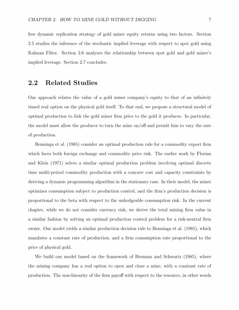
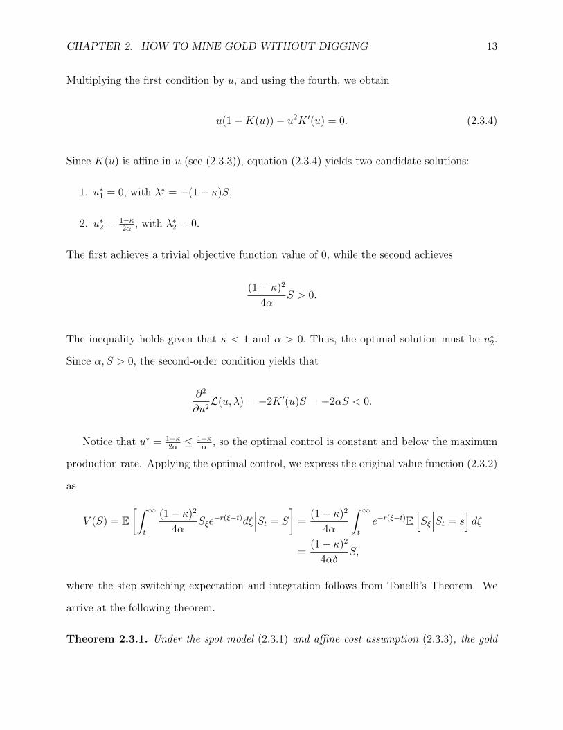
The gold miner’s equity is a function of the physical gold price. As a consequence, the
equity J can be perfectly replicated using a portfolio of ∂J∂S
shares of physical gold and the
rest composed of the money market account. Figure 1 illustrates the value of the gold miner
equity compared to the immediate value of paying back the debt under different spot prices
for gold. As we can see, the value function is convex and approaches the asset value less
debt as the price of gold surpasses S∗. Under this model the gold miner’s equity can always
be spanned by some combination of physical gold and the money market account. Although
CHAPTER 2. HOW TO MINE GOLD WITHOUT DIGGING 18
0.0 0.2 0.4 0.6 0.8 1.0Gold Price (S)
0.70
0.75
0.80
0.85
0.90
0.95
1.00
J(S)
J(S)Exercise Value
Figure 1: The value function J(S) (blue) and the immediate exercise value(1−κ)2
4αδ St − D (red) vs the spot price of gold S. The parameters are α = 0.2,κ = 0.95, r = 0.02, δ = 0.01, σ = 0.1, D = 0.33, C = 0.015. The optimal exerciselevel is S∗ = 0.38.
this result seems surprising, we will demonstrate in Section 2.4 that 70% of the gold miner
equity returns can be explained by a tradable replicating portfolio consisting only of the
equity market portfolio, risk free bonds, and physical gold. Thus, although replication is far
from perfect, by buying the correct dynamic quantities of gold and risk-free bonds, we have
thus managed to “mine gold without digging!”
2.3.3 Comparative Statics
We now set up the framework for our empirical asset pricing model by considering how the
dynamic quantities of physical gold we need for replication vary with respect to time. In
particular, since we care about comparing returns of the various assets in our sample, it
is important to analyze how the implied leverage of the gold miner equity with respect to
gold varies over time. The instantaneous return of the gold mining equity is related to the
instantaneous returns of the physical gold and the money market account as follows:
dJtJt
= β(St)dStSt
+ (1− β(St))rdt.

CHAPTER 2. HOW TO MINE GOLD WITHOUT DIGGING 19
In the non-trivial continuation region St = S ≤ S∗, we have
β(S) =∂J
∂S
S
J=
AγSγ
ASγ − 4αδCr(1−κ)2
(2.3.7)
We call β(S) the implied gold leverage of the gold miner equity, choosing to suppress
the time dependence for notational simplicity. When β is larger, the equity is more risky
with higher risk premium and hence has lower price, and when β is smaller, the equity is less
risky with lower risk premium and hence has higher price. We would like to understand how
the gold miner implied leverage varies with the various explicit parameters of our company.
Proposition 1. In the continuation region where S ≤ S∗, the sensitivities of the implied
gold leverage with respect to the gold price are given by
β′(S) =− 4αδC
(1−κ)2r(ASγ − 4αδC
(1−κ)2r
)2 < 0, β′′(S) = −2β
S× β′(S) > 0.
Furthermore, the stochastic evolution of the implied gold leverage β(St) follows
dβ(St) = β′(St)dSt +1
2β′′(St)(dSt)
2
= β′(St)(dSt − βσ2Stdt
). (2.3.8)
Our model confirms a number of financial intuitions. As the spot gold price increases, the
implied leverage of the gold company falls. Furthermore, the implied leverage is decreasing
convex in the gold price S, so a higher price of physical gold decreases leverage by a smaller
and smaller amount as S → ∞. On the other hand, a fall in gold price would lead to
implied leverage spiraling higher and higher by the same convexity property. By a replicating
portfolio argument, we can imagine that a higher (relative) cost gold miner company borrows
more in order to fund his positions in the physical gold, and as costs increase more and more
CHAPTER 2. HOW TO MINE GOLD WITHOUT DIGGING 20
0.20 0.25 0.30 0.35 0.40 0.45 0.50 0.55 Marginal Cost
2.0
2.5
3.0
3.5
4.0
GLD
0.88 0.89 0.90 0.91 0.92 0.93 Fixed Cost
1.75
2.00
2.25
2.50
2.75
3.00
3.25
3.50
GLD
1 2 3 4 5Gold Price
1.5
2.0
2.5
3.0
3.5
4.0
GLD
0.10 0.15 0.20 0.25 0.30 0.35 0.40 0.45Debt/Equity Ratio
1.6
1.7
1.8
1.9
2.0
GLD
0.020 0.025 0.030 0.035 0.040 0.045 0.050Interest Rate
1.3
1.4
1.5
1.6
1.7
1.8
GLD
0.0 0.1 0.2 0.3 0.4 0.5 0.6 0.7 0.8Gold Volatility
1.3
1.4
1.5
1.6
1.7
1.8
1.9
2.0
2.1
GLD
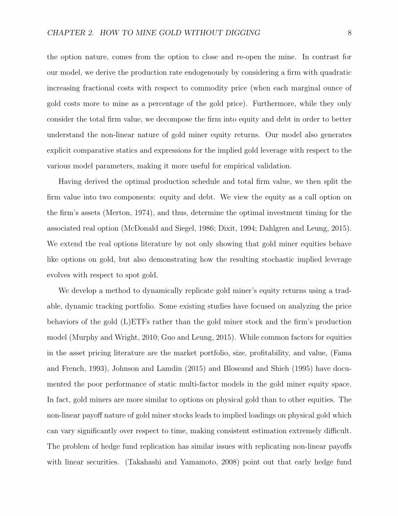
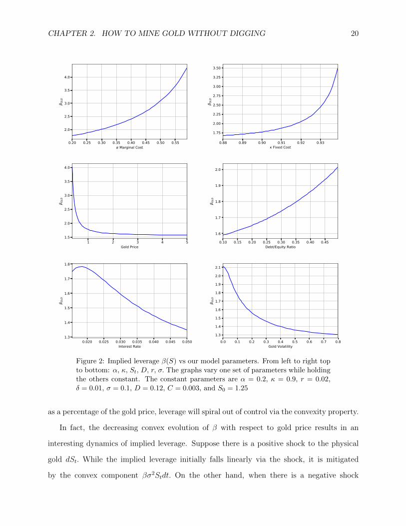
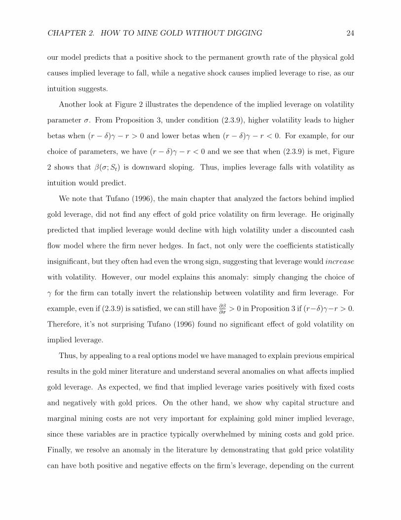
Figure 2: Implied leverage β(S) vs our model parameters. From left to right topto bottom: α, κ, St, D, r, σ. The graphs vary one set of parameters while holdingthe others constant. The constant parameters are α = 0.2, κ = 0.9, r = 0.02,δ = 0.01, σ = 0.1, D = 0.12, C = 0.003, and S0 = 1.25
as a percentage of the gold price, leverage will spiral out of control via the convexity property.
In fact, the decreasing convex evolution of β with respect to gold price results in an
interesting dynamics of implied leverage. Suppose there is a positive shock to the physical
gold dSt. While the implied leverage initially falls linearly via the shock, it is mitigated
by the convex component βσ2Stdt. On the other hand, when there is a negative shock
CHAPTER 2. HOW TO MINE GOLD WITHOUT DIGGING 21
to the physical gold price, then implied leverage increases even more through the convex
component. Therefore, the convexity of beta acts as an anti-regulatory mechanism for high
cost gold producers: even a small decrease in gold prices can cause a massive increase in
implied leverage! Moreover, the implied leverage of a high-cost mining company should be
extremely volatile and hence more difficult to estimate vs the implied leverage of a lower
cost mining company.
On the other hand, as the cost parameters κ and α rise, the implied leverage of the gold
company will increase as well, a mirror result to Proposition 1.
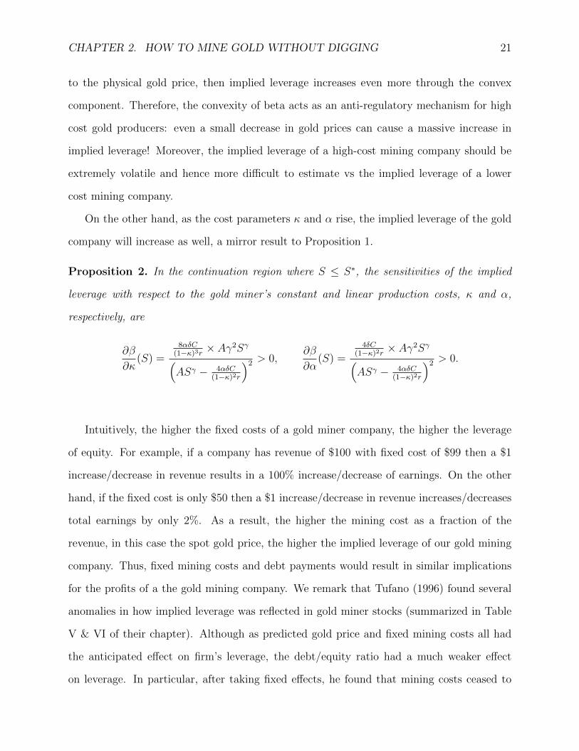
Proposition 2. In the continuation region where S ≤ S∗, the sensitivities of the implied
leverage with respect to the gold miner’s constant and linear production costs, κ and α,
respectively, are
∂β
∂κ(S) =
8αδC(1−κ)3r
× Aγ2Sγ(ASγ − 4αδC
(1−κ)2r
)2 > 0,∂β
∂α(S) =
4δC(1−κ)2r
× Aγ2Sγ(ASγ − 4αδC
(1−κ)2r
)2 > 0.
Intuitively, the higher the fixed costs of a gold miner company, the higher the leverage
of equity. For example, if a company has revenue of $100 with fixed cost of $99 then a $1
increase/decrease in revenue results in a 100% increase/decrease of earnings. On the other
hand, if the fixed cost is only $50 then a $1 increase/decrease in revenue increases/decreases
total earnings by only 2%. As a result, the higher the mining cost as a fraction of the
revenue, in this case the spot gold price, the higher the implied leverage of our gold mining
company. Thus, fixed mining costs and debt payments would result in similar implications
for the profits of a the gold mining company. We remark that Tufano (1996) found several
anomalies in how implied leverage was reflected in gold miner stocks (summarized in Table
V & VI of their chapter). Although as predicted gold price and fixed mining costs all had
the anticipated effect on firm’s leverage, the debt/equity ratio had a much weaker effect
on leverage. In particular, after taking fixed effects, he found that mining costs ceased to
CHAPTER 2. HOW TO MINE GOLD WITHOUT DIGGING 22
be significant. In other words, while fixed mining costs were important, increased marginal
costs had less effects on leverage. By appealing to our real options model of the gold mining
firm, we can explain why they found such anomalies in the determinants of firm leverage.
Figure 2 illustrates the dependence of the gold miner equity’s implied leverage on various
model parameters. As predicted by Proposition 1, the leverage increases significantly as the
gold price reaches a significant threshold, in this case around 0.5 times the original value S0.
Similarly, Proposition 2 predicts a similar “convexity” effect as both the fixed percentage cost
κ and the marginal percentage cost α increases. For example, a small increase of 0.06 in the
fixed cost results in leverage rising from 1.6 to 3.5. On the other hand, rises in the marginal
cost α result in much less dramatic increases in the leverage. We need to almost triple α in
order to generate the same rise in leverage. The intuition is that a larger fixed cost cannot
be accommodated easily, while changes in marginal costs are usually offset by an increase in
the gold price itself. After all, one would only choose to mine the high cost of production
gold if the gold price itself was high! Finally, changes in the debt/equity structure leads to
only moderate changes in implied leverage compared to changes in the mining costs. This is
because typically most of the fixed costs of a gold miner are related to mining costs for the
gold rather than payments of coupons for the bondholders, so the capital structure is less
important than the mining cost structure. For example, Jorion (2006) reveals that the net
profit margin for oil and gas drilling companies is typically 5%, suggesting that over 90% of
the cost can be attributed to fixed costs and not coupon payments.
Furthermore, we can consider the variation of the gold miner implied leverage with respect
to the implied growth parameters of our model.
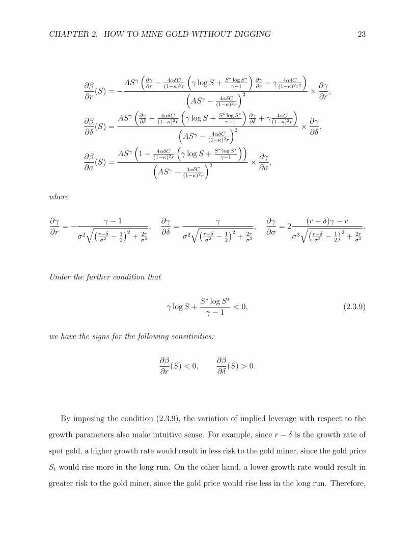
Proposition 3. In the continuation region where S ≤ S∗, the sensitivities for the implied
leverage with respect to the model parameters, namely, the interest rate r, net convenience
yield δ, and volatility σ of the spot gold price, respectively, are given by
CHAPTER 2. HOW TO MINE GOLD WITHOUT DIGGING 23
∂β
∂r(S) = −
ASγ(∂γ∂r− 4αδC
(1−κ)2r
(γ logS + S∗ logS∗
γ−1
)∂γ∂r− γ 4αδC
(1−κ)2r2
)(ASγ − 4αδC
(1−κ)2r
)2 × ∂γ
∂r,
∂β
∂δ(S) =
ASγ(∂γ∂δ− 4αδC
(1−κ)2r
(γ logS + S∗ logS∗
γ−1
)∂γ∂δ
+ γ 4αC(1−κ)2r
)(ASγ − 4αδC
(1−κ)2r
)2 × ∂γ
∂δ,
∂β
∂σ(S) =
ASγ(
1− 4αδC(1−κ)2r
(γ logS + S∗ logS∗
γ−1
))(ASγ − 4αδC
(1−κ)2r
)2 × ∂γ
∂σ,
where
∂γ
∂r= − γ − 1
σ2
√(r−δσ2 − 1
2
)2+ 2r
σ2
,∂γ
∂δ=
γ
σ2
√(r−δσ2 − 1
2
)2+ 2r
σ2
,∂γ
∂σ= 2
(r − δ)γ − rσ3
√(r−δσ2 − 1
2
)2+ 2r
σ2
.
Under the further condition that
γ logS +S∗ logS∗
γ − 1< 0, (2.3.9)
we have the signs for the following sensitivities:
∂β
∂r(S) < 0,
∂β
∂δ(S) > 0.
By imposing the condition (2.3.9), the variation of implied leverage with respect to the
growth parameters also make intuitive sense. For example, since r − δ is the growth rate of
spot gold, a higher growth rate would result in less risk to the gold miner, since the gold price
St would rise more in the long run. On the other hand, a lower growth rate would result in
greater risk to the gold miner, since the gold price would rise less in the long run. Therefore,
CHAPTER 2. HOW TO MINE GOLD WITHOUT DIGGING 24
our model predicts that a positive shock to the permanent growth rate of the physical gold
causes implied leverage to fall, while a negative shock causes implied leverage to rise, as our
intuition suggests.
Another look at Figure 2 illustrates the dependence of the implied leverage on volatility
parameter σ. From Proposition 3, under condition (2.3.9), higher volatility leads to higher
betas when (r − δ)γ − r > 0 and lower betas when (r − δ)γ − r < 0. For example, for our
choice of parameters, we have (r − δ)γ − r < 0 and we see that when (2.3.9) is met, Figure
2 shows that β(σ;St) is downward sloping. Thus, implies leverage falls with volatility as
intuition would predict.
We note that Tufano (1996), the main chapter that analyzed the factors behind implied
gold leverage, did not find any effect of gold price volatility on firm leverage. He originally
predicted that implied leverage would decline with high volatility under a discounted cash
flow model where the firm never hedges. In fact, not only were the coefficients statistically
insignificant, but they often had even the wrong sign, suggesting that leverage would increase
with volatility. However, our model explains this anomaly: simply changing the choice of
γ for the firm can totally invert the relationship between volatility and firm leverage. For
example, even if (2.3.9) is satisfied, we can still have ∂β∂σ> 0 in Proposition 3 if (r−δ)γ−r > 0.
Therefore, it’s not surprising Tufano (1996) found no significant effect of gold volatility on
implied leverage.
Thus, by appealing to a real options model we have managed to explain previous empirical
results in the gold miner literature and understand several anomalies on what affects implied
gold leverage. As expected, we find that implied leverage varies positively with fixed costs
and negatively with gold prices. On the other hand, we show why capital structure and
marginal mining costs are not very important for explaining gold miner implied leverage,
since these variables are in practice typically overwhelmed by mining costs and gold price.
Finally, we resolve an anomaly in the literature by demonstrating that gold price volatility
can have both positive and negative effects on the firm’s leverage, depending on the current
CHAPTER 2. HOW TO MINE GOLD WITHOUT DIGGING 25
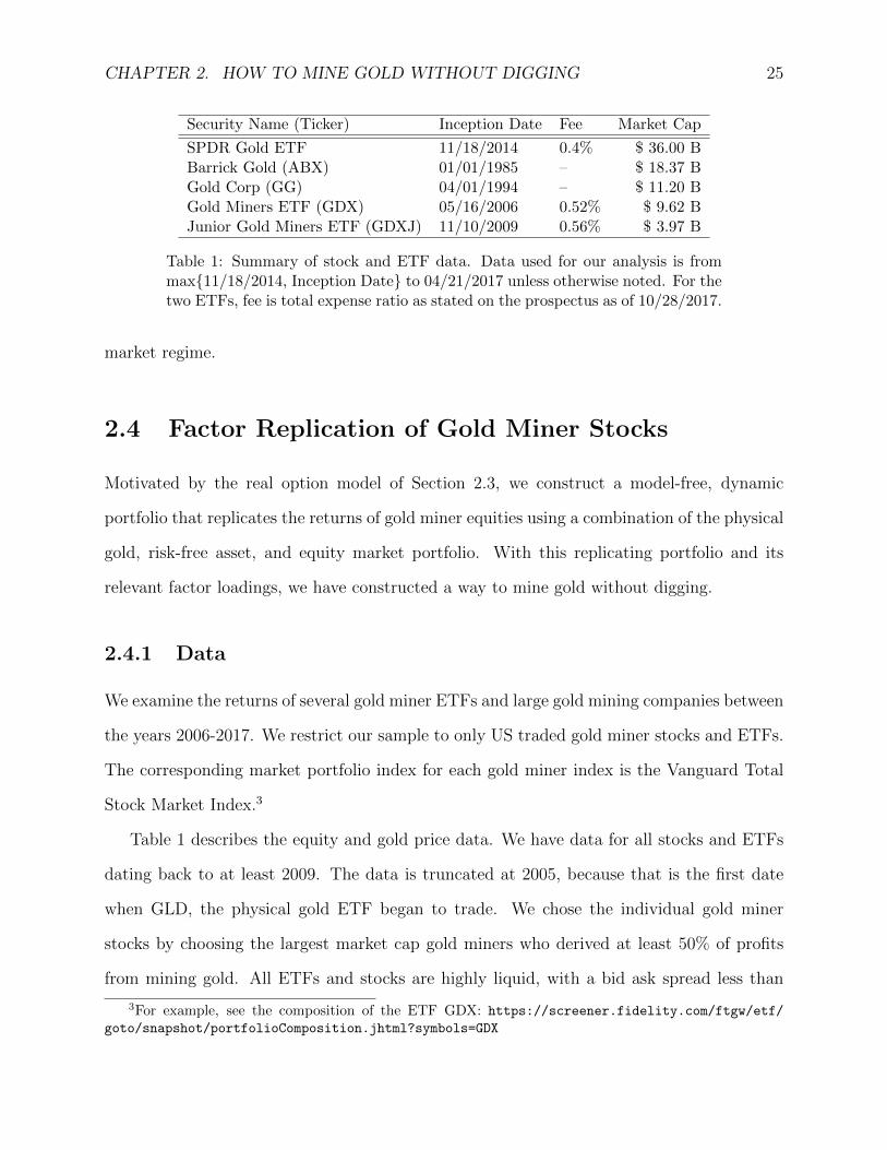
Security Name (Ticker) Inception Date Fee Market Cap
SPDR Gold ETF 11/18/2014 0.4% $ 36.00 BBarrick Gold (ABX) 01/01/1985 – $ 18.37 BGold Corp (GG) 04/01/1994 – $ 11.20 BGold Miners ETF (GDX) 05/16/2006 0.52% $ 9.62 BJunior Gold Miners ETF (GDXJ) 11/10/2009 0.56% $ 3.97 B
Table 1: Summary of stock and ETF data. Data used for our analysis is frommax11/18/2014, Inception Date to 04/21/2017 unless otherwise noted. For thetwo ETFs, fee is total expense ratio as stated on the prospectus as of 10/28/2017.
market regime.
2.4 Factor Replication of Gold Miner Stocks
Motivated by the real option model of Section 2.3, we construct a model-free, dynamic
portfolio that replicates the returns of gold miner equities using a combination of the physical
gold, risk-free asset, and equity market portfolio. With this replicating portfolio and its
relevant factor loadings, we have constructed a way to mine gold without digging.
2.4.1 Data
We examine the returns of several gold miner ETFs and large gold mining companies between
the years 2006-2017. We restrict our sample to only US traded gold miner stocks and ETFs.
The corresponding market portfolio index for each gold miner index is the Vanguard Total
Stock Market Index.3
Table 1 describes the equity and gold price data. We have data for all stocks and ETFs
dating back to at least 2009. The data is truncated at 2005, because that is the first date
when GLD, the physical gold ETF began to trade. We chose the individual gold miner
stocks by choosing the largest market cap gold miners who derived at least 50% of profits
from mining gold. All ETFs and stocks are highly liquid, with a bid ask spread less than
3For example, see the composition of the ETF GDX: https://screener.fidelity.com/ftgw/etf/
goto/snapshot/portfolioComposition.jhtml?symbols=GDX
CHAPTER 2. HOW TO MINE GOLD WITHOUT DIGGING 26
5 bps and a market capitalization greater than $1 billion throughout the entire sampling
period. Finally, we use the 3M LIBOR rate as the risk-free rate in our calculations. All price
data was obtained from Quandl, but at the money implied volatility estimates for gold were
taken from Bloomberg.
2.4.2 Constructing the Replicating Portfolio
Intuitively, gold miner returns should have significant correlation with both gold returns and
the market returns. However, since Section 2.3 suggests that all gold miner stocks are related
to real gold options, leverage with respect to gold price varies over time. Since firm leverage
should increase when gold prices fall closer to production cost, a pooled regression would
ignore the time series variation in firm leverage. Thus, it is not sensible to use a standard
pooled regression over the whole sample space to estimate a firm’s exposure to gold price as
preferred under the asset pricing literature. On the other hand, since the (variable) price of
gold is much more volatile than (fixed) production costs, the variation of firm leverage with
respect to gold must vary substantially, even over short time periods. Therefore, we will
must infer βGLD, the firm’s implied gold leverage, through short-window rolling regressions.
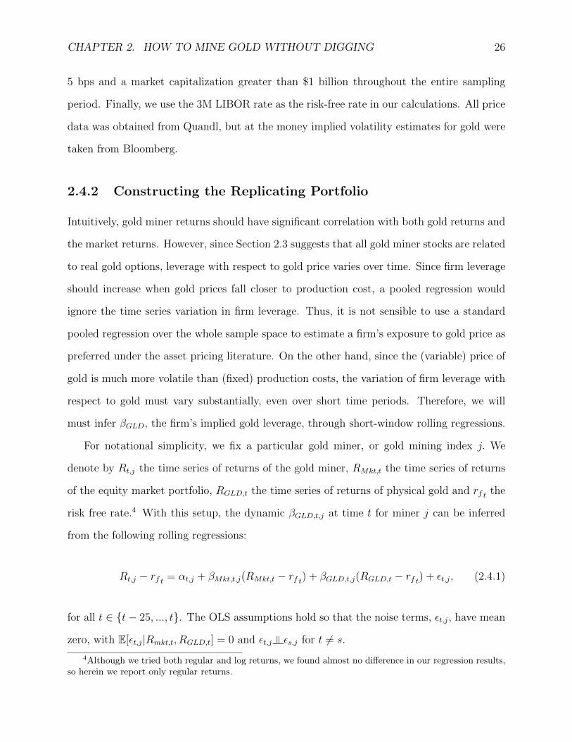
For notational simplicity, we fix a particular gold miner, or gold mining index j. We
denote by Rt,j the time series of returns of the gold miner, RMkt,t the time series of returns
of the equity market portfolio, RGLD,t the time series of returns of physical gold and rf t the
risk free rate.4 With this setup, the dynamic βGLD,t,j at time t for miner j can be inferred
from the following rolling regressions:
Rt,j − rf t = αt,j + βMkt,t,j(RMkt,t − rf t) + βGLD,t,j(RGLD,t − rf t) + εt,j, (2.4.1)
for all t ∈ t− 25, ..., t. The OLS assumptions hold so that the noise terms, εt,j, have mean
zero, with E[εt,j|Rmkt,t, RGLD,t] = 0 and εt,j |= εs,j for t 6= s.
4Although we tried both regular and log returns, we found almost no difference in our regression results,so herein we report only regular returns.

CHAPTER 2. HOW TO MINE GOLD WITHOUT DIGGING 27
We regress the excess returns of the gold miner on the excess returns of the equity market
portfolio and the excess return of gold over a time period of length 25 business days going
backwards from the time point t. Our regression uses exponential weightings with the decay
parameter λ = 0.95 so as to weigh the closer time points more due to the time varying nature
of βGLD,t,j. The regression factor coefficients, αt,j, βMkt,t,j and βGLD,t,j depend on the time
t where the regression time series ends, and the gold miner equity j whose returns we are
trying to explain. In particular, the gold coefficients βGLD,t,j represent an estimation of the
instantaneous elasticity of the gold miner stock with respect to gold price. However, unlike
the coefficients of (2.3.8), so far we place no constraints on βGLD besides the standard OLS
assumptions. Later in Section 2.5, we will show a way to combine the real options model
of Proposition 1 with our regression estimates to produce model consistent and efficient
estimations of time varying implied gold leverage.
Recall that the real options of Section 2.3 implies that a time-varying portfolio in physical
gold would explain the returns of gold miner stocks. In addition, since gold miner stocks
generally exhibit positive covariance with the stock market, we should observe a significant
loading on the market portfolio as well. Therefore, if our model is correctly specified, then
the average α should be zero, with positive βGLD and βMkt coefficients. Note that while
this procedure assumes that the replicating portfolio is dynamic with respect to the factor
loadings, it does not assume a payoff or specific structural form for the real option we are
trying to calibrate. That is why we consider the replicating portfolio construction to be
“model-free.”
Having calculated the localized factor loadings for each gold miner on physical gold, we
are now ready to construct the replicating portfolio. From our model free formulation, under
the assumption that αt,j ≡ 0, we expect that a portfolio with weights of βGLD,t,j in the GLD
ETF, βMkt,t,j in the market portfolio, and 1− βGLD,t,j − βMkt,t,j in the risk free asset should
exactly replicate Rt,j, the return of the gold miner at time t. Of course, unless R2 ≡ 1 exactly,
we will not have perfect replication, only replication on average. Finally, we must lag our

CHAPTER 2. HOW TO MINE GOLD WITHOUT DIGGING 28
Security Name (Ticker) R2 α βportfolio
Barrick Gold (ABX) 0.609360 −0.003494∗ 0.895739∗∗
Goldcorp (GG) 0.626465 −0.003983∗ 0.916772∗∗
Gold Miners ETF (GDX) 0.715839 −0.005844∗∗ 0.874759∗∗
Junior Gold Miners ETF (GDXJ) 0.634395 −0.008139∗∗ 0.821515∗∗∗
Table 2: Performance of the replicating portfolio constructed with weightsβGLD,t,j and βMkt,j at each time t for equity j on a monthly frequency. Thesefactor loadings are obtained via the regression (2.4.1). The table shows the re-sult of the two sided t-test for αj 6= 0 and βportfolio,j 6= 1. Hull-white standarderrors were used to calculate t-statistics. The symbols *, **, and *** indicatesignificance at the 10%, 5% and 1% levels respectively for each test.
regression coefficients by one time period to ensure that the portfolio construction method
only uses information available at time t.
Thus, at time t, with ∆t = 1 week, we form a portfolio which consists of weights
ωt,j = (βGLD,t−∆t,j, βMkt,t−∆t,j, 1− βGLD,t−∆t,j − βMkt,t−∆t,j)
in the physical gold, market portfolio, and risk-free asset respectively. At time t + ∆t, the
portfolio will have a mark-to-market return of
Rt,j,portfolio = ω′t,j(Rt,GLD, Rt,Mkt, rf t).
Furthermore, since the gold miner’s dependence on the market portfolio (equity market beta)
should not be time varying, we simply set the time average of the βMkt,j coefficients at all
times t, thereby removing the dependence on t. Having constructed the replicating portfolio,
we can test its success by running the regression
Rt,j = βportfolio,jRt,j,portfolio + αj + εt,j. (2.4.2)
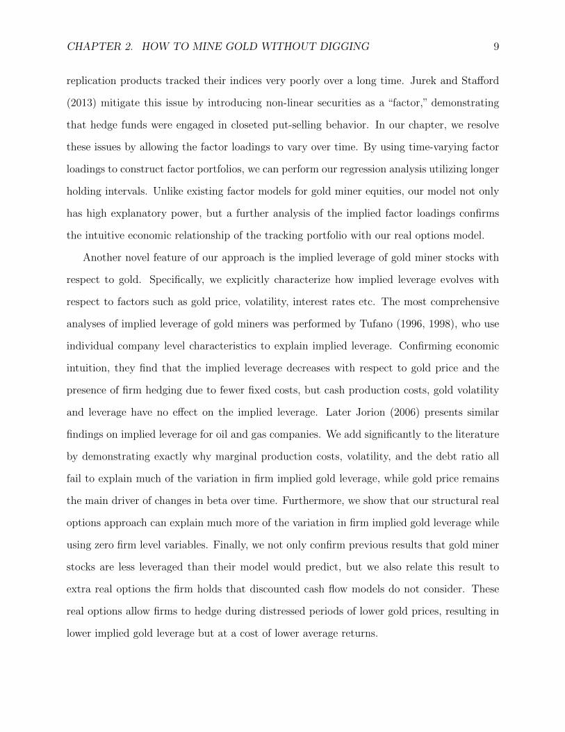
Table 2 shows the result of our regression analysis with respect to our replicating portfolio,
while Figure 3 demonstrates the goodness of fit of our replicating portfolio model. First, we
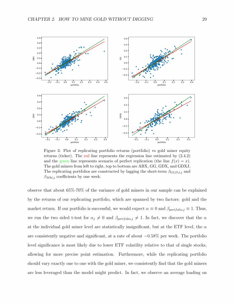
CHAPTER 2. HOW TO MINE GOLD WITHOUT DIGGING 29
0.2 0.1 0.0 0.1 0.2 0.3 0.4 0.5portfolio
0.3
0.2
0.1
0.0
0.1
0.2
0.3
0.4
0.5
ABX
0.2 0.1 0.0 0.1 0.2 0.3 0.4portfolio
0.2
0.1
0.0
0.1
0.2
0.3
0.4
GG
0.2 0.1 0.0 0.1 0.2 0.3 0.4portfolio
0.2
0.1
0.0
0.1
0.2
0.3
0.4
GDX
0.2 0.1 0.0 0.1 0.2 0.3portfolio
0.2
0.1
0.0
0.1
0.2
0.3
GDXJ
Figure 3: Plot of replicating portfolio returns (portfolio) vs gold miner equityreturns (ticker). The red line represents the regression line estimated by (2.4.2)and the green line represents scenario of perfect replication (the line f(x) = x).The gold miners from left to right, top to bottom are ABX, GG, GDX, and GDXJ.The replicating portfolios are constructed by lagging the short-term βGLD,t,j andβMkt,j coefficients by one week.
observe that about 65%-70% of the variance of gold miners in our sample can be explained
by the returns of our replicating portfolio, which are spanned by two factors: gold and the
market return. If our portfolio is successful, we would expect α ≡ 0 and βportfolio,j ≡ 1. Thus,
we run the two sided t-test for αj 6= 0 and βportfolio,j 6= 1. In fact, we discover that the α
at the individual gold miner level are statistically insignificant, but at the ETF level, the α
are consistently negative and significant, at a rate of about −0.58% per week. The portfolio
level significance is most likely due to lower ETF volatility relative to that of single stocks,
allowing for more precise point estimation. Furthermore, while the replicating portfolio
should vary exactly one to one with the gold miner, we consistently find that the gold miners
are less leveraged than the model might predict. In fact, we observe an average loading on

CHAPTER 2. HOW TO MINE GOLD WITHOUT DIGGING 30
the portfolio of less than 0.90.
How can we explain the consistently negative α and low covariation with the replicating
portfolio? Suppose that the firm owns a real option which they choose to exercise when
they observe their stock covaries too much with gold prices. In practice, gold miners could
buy put options, sell longer term futures or cut costs by firing workers and closing down
mines. By exercising these options, the firm would in fact execute a regime change, so that
the magnitude of the previously estimated implied leverage coefficient βGLD,t,j would become
too large relative to the actual future βGLD,t+∆t,j. Because the replicating portfolio cannot
fully internalize this regime change for at least 25 business days (the length of our rolling
training samples), the portfolio construction method would lead to portfolios which are too
leveraged with respect to physical gold. However, hedging gold price risk is quite costly; if
the managers do not have superior information about future gold prices then any hedging
will result in a negative alpha penalty.
Figure 3 compares the difference between the anticipated relationship of full replication
(green line) vs the actual performance of the replicating portfolio (red line). In particu-
lar, we find that the replicating portfolio declines moderately more than the actual gold
miner during periods of negative gold returns, while the replicating portfolio significantly
outperforms during periods of high gold prices. In other words, firms sacrifice large upward
potential gains when gold prices gain in exchange for small relative gains when gold prices
fall, suggesting that the cost of reducing leverage is paid through negative alpha relative to
the replicating portfolio Finally, since gold has on average a positive return during the period
under consideration, then the effects of holding and exercising these additional real options
ends up generating a small negative alpha!
CHAPTER 2. HOW TO MINE GOLD WITHOUT DIGGING 31
2.5 Estimating Model Parameters with Kalman Filter
In this section we present an application of our model, focusing on estimating the firm
implied gold leverage parameters from the replicating portfolio for our model. In particular,
we demonstrate a way to smooth the estimated dynamic factor loadings from Section 2.4 by
estimating a Kalman Filter derived from the real options framework of Section 2.3.
So far, we have constructed a procedure to replicate the returns of gold miner equity
prices, using only information which was available at the time of portfolio construction.
Moreover, under the real options model, this portfolio should contain time-varying loadings
on physical gold. Previously, we estimated these dynamic loadings using short-term rolling
linear regressions. However, due to the low number of observations per rolling window,
although estimation is consistent under OLS assumptions, the estimator on βGLD has extreme
variation. In this section, we demonstrate how under the real options model, the factor
loadings follow a linear update rule, which allows us to smooth the OLS estimates with a
Kalman Filter. Thus, by constraining the evolution of βGLD to obey the real options model
of Section 2.3, we obtain a more efficient estimator of the factor loadings.
Let St denote the gold price again, and assume we only have one gold miner stock.
In order to analyze the implied gold leverage dynamics of gold miner stocks, we need to
have an accurate estimate of the time series βGLD,t ≡ β(St), over t ≥ 0. While our short
rolling regressions can generate estimates of β(St), the estimates are extremely noisy and
vary quite substantially over even a single week. Therefore, we wish to extract the true β(St)
by estimating the noisy parameters zti ≡ β(Sti) with short-window rolling regressions. We
do this by reframing our model within the context of the Extended Kalman Filter (see e.g.
Brown and Hwang (1997) for a description of the Kalman Filter.)
Suppose that the true model for β(St) follows (2.3.8). Discretizing the Ito process for
CHAPTER 2. HOW TO MINE GOLD WITHOUT DIGGING 32
β(St),
dβ(St) = β′(St)(dSt − βσ2Stdt
),
β(Sti) = β(Sti−1) + β′(Sti−1
)×(∆Sti − β(Sti−1
)σ2Sti−1∆t). (2.5.1)
At time ti, the variables β(Sti−1), ∆Sti , β(Sti−1
), and Sti−1are all known. We take σ2, the
volatility of the gold price, as the implied volatility of an ATM 3M to maturity gold futures
option and ∆t ≡ 1/252. It remains to calculate β′(St−1). Applying Ito’s Formula to β(S)
reveals
dβ′(St) = β(St)β′(St)
(−2
dStSt
+ σ2(2β(St) + 1)dt
)− σ2St (β′(St))
2dt
β′(Sti) = β′(Sti−1) + β(Sti−1
)β′(Sti−1)
(−2
∆StiSti−1
+ σ2(2β(Sti−1) + 1)∆t
)− σ2Sti−1
(β′(Sti−1
))2
∆t
Thus, we can define a state vector x, with white noise N (0, Qti) where
xti =(βSti , β
′(Sti))T,
Qti=
S2ti
−2β(Sti)Sti
−2β(Sti)Sti 4β(Sti)2
× (β′(Sti))2σ2∆t.
In other words, we choose the betas and partials of betas with respect to the gold price as our
state space x. Each state evolves with error equal to the instantaneous quadratic covariation
of the process Q. Finally, the predicted update function f(x) is given by (2.5.1).
Define the 2× 2 covariance transition matrix, the 2× 1 observation matrix, and the 1× 1

CHAPTER 2. HOW TO MINE GOLD WITHOUT DIGGING 33
observation error matrix as
Fti =
1− β′(Sti)σ2Sti∆t ∆Sti − β(Sti)σ
2Sti∆t
β′(Sti)(−2
∆StiSti
+ σ2(4β(Sti) + 1)∆t)
1 + β(Sti)(−2
∆StiSti
+ σ2(2β(Sti) + 1)∆t)
−2σ2Stiβ′(Sti)∆t
Hti = (1, 0)T
Rti = Standard Error2βGLD
(ti).
In other words, F is an updating matrix for the covariance matrix of errors, assuming our
model and state space specification is correct. H reflects the fact that only β(St) is observable
through our short-window rolling regressions, while β′(St) remains a latent variable. Finally,
we choose the scalar measurement error R to be the standard error attached to the estimates
of β(St) from our rolling regressions (2.4.1). Thus, the Kalman Filter procedure is
Predict
Predicted state estimate: xti|ti−1= f(xti−1|ti−1
),
Predicted covariance estimate: Pti|ti−1= Fti−1
Pti−1|ti−1FTti−1
+ Qti−1,
Update
Innovation or measurement residual: yti = zti −HTtixti|ti−1
,
Innovation (or residual) covariance: Si = HTtiPti|ti−1
Hti + Rti ,
Near-optimal Kalman gain: Kti = Pti|ti−1HtiS
−1ti,
Updated state estimate: xti|ti = xti|ti−1+ Kiyti ,
Updated covariance estimate: Pti|ti = Pti|ti−1(I−HtiK
Tti
),
where x is the (possibly hidden) state variable, f is the state update equation, Q is the
CHAPTER 2. HOW TO MINE GOLD WITHOUT DIGGING 34
covariance matrix of the state variables, H is the observation matrix, F is the covariance
update matrix, and R is the estimation error, all of which as previously defined.
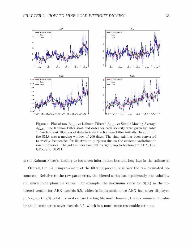
Having defined all the parameters of the Kalman Filter, we apply the filtering procedure
at a daily frequency over the observed lifetime of our various ETFs and gold miner stocks
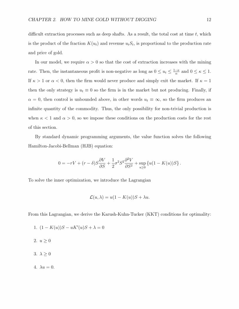
(see Table 1 for a list of inception dates.) Figure 4 compares the improvement of the Kalman
Filtered implied leverage time series and the simple moving average (SMA) smoothed time
series over the raw regression coefficients. For the SMA model, we experimented with dif-
ferent moving time windows, settling on a window of 200 days so that the SMA coefficients
have a similar degree of volatility as the filtered estimates. While we did experiment with
shorter windows, we found that the resulting series was too similar to the original raw time
series, necessitating longer smoothing windows for the SMA method.
First, note that the SMA coefficients are less volatile than the raw estimated parameters.
While SMA gains in less volatility relative to the raw estimates, it loses in missing information
to the filtered estimates. For example in mid-2013, gold prices fell and the implied leverage
of gold mining firms rose to an all time high. The Kalman Filter captures the regime change
in 2013 almost immediately, but the SMA model does not pick it up until the beginning of
2014. In addition, for GDX and GDXJ the SMA model misses a regime change in mid-2009
when gold prices rose while the Kalman Filter picks it up much faster. Therefore, while long
window SMA smoothers are less complex and adequate substitutes during times of stable
gold prices, the Kalman Filter outperforms when gold prices are more volatile, since it can
capture instantaneous changes in implied leverage.
However, most of the time there is not a huge difference between the Kalman Filtered
implied leverage coefficients and SMA smoothed parameters, as long as we use a long enough
window. The main advantage of the Kalman Filter over simple smoothing methods is that it
not only infers the true process for βGLD, but it also preserves some volatility of our dynamic
factor loadings. On the other hand, while the SMA procedure certainly is less complex and
less prone to model risk, it requires a very long window to generate an estimate as smooth
CHAPTER 2. HOW TO MINE GOLD WITHOUT DIGGING 35
2006 2008 2010 2012 2014 2016
1
2
3
4
5
6ABX
Kalman FilterRawSMA
2006 2008 2010 2012 2014 20160
1
2
3
4
GGKalman FilterRawSMA
2007 2008 2009 2010 2011 2012 2013 2014 2015 20160.5
1.0
1.5
2.0
2.5
3.0
3.5
4.0
4.5GDX
Kalman FilterRawSMA
2010 2011 2012 2013 2014 2015 2016
1
2
3
4
5
GDXJKalman FilterRawSMA
Figure 4: Plot of raw βGLD vs Kalman Filtered βGLD vs Simple Moving AverageβGLD. The Kalman Filter start end dates for each security were given by Table1. We hold out 100-days of data to train the Kalman Filter initially. In addition,the SMA uses a moving window of 200 days. The time axis has been convertedto weekly frequencies for illustration purposes due to the extreme variations inraw time series. The gold miners from left to right, top to bottom are ABX, GG,GDX, and GDXJ.
as the Kalman Filter’s, leading to too much information loss and long lags in the estimates.
Overall, the main improvement of the filtering procedure is over the raw estimated pa-
rameters. Relative to the raw parameters, the filtered series has significantly less volatility
and much more plausible values. For example, the maximum value for β(St) in the un-
filtered version for ABX exceeds 5.5, which is implausible since ABX has never displayed
5.5×σGLD ≈ 60% volatility in its entire trading lifetime! However, the maximum such value
for the filtered series never exceeds 3.5, which is a much more reasonable estimate.
CHAPTER 2. HOW TO MINE GOLD WITHOUT DIGGING 36
2.6 Testing Predictions for Gold Miners’ Implied Lever-
age
In this section we analyze the accuracy of the predictions made by the real options model for
gold miners as applied to our gold miner stock portfolio, focusing on our model’s explanatory
power of firm implied gold leverage. We perform an empirical test of our real options model
by analyzing the effect of gold prices on firm leverage, using monthly observations of the
filtered estimates for the β(St) estimates. Overall, we find that the real options model can
explain much of the time series variation of implied gold leverage, suggesting that gold miner
stocks really do behave like real options on gold.
Having developed a method to robustly estimate the factor loadings themselves, we can
now empirically investigate our model’s predictions about how changes in gold prices affect
firm leverage. In particular, recall that at each time t, we have inferred firm j’s dependence
on gold prices βGLD,t,j by carrying out a rolling, exponentially weighted regression (2.4.1).
Now that we have an unbiased, smoothed estimate of the implied leverage parameters via
the Kalman Filter, we can test how the firm leverage depends on gold prices, as our real
options model would predict. Figure 5 illustrates this relationship for the four gold miner
ETFs/stocks in our sample. Notice that in most circumstances, the relationship between
physical gold prices and the firm implied gold leverage is quite muted, with βGLD varying
around some constant level. However, as the gold price declines past a critical level, firm
price declines and leverage increases rapidly. Similarly, around this critical level, when the
gold price increases, the firm price decreases and the leverage falls rapidly as well. Recall
that Figure 2 predicts that the firm’s implied gold leverage only becomes extremely sen-
sitive around the critical gold price which pushes the firm close to default. Thus, these
summary figures suggest that our real options model should have strong explanatory power
for understanding gold miners’ implied leverage.
While the general pattern between gold prices and firm implied leverage can be eyeballed

CHAPTER 2. HOW TO MINE GOLD WITHOUT DIGGING 37
20062008
20102012
20142016
40
60
80
100
120
140
160
180
GLD
Price
1.0
1.5
2.0
2.5
3.0
3.5
GLD
ABX
20062008
20102012
20142016
40
60
80
100
120
140
160
180
GLD
Price
0.5
1.0
1.5
2.0
2.5
3.0
GLD
GG
20072008
20092010
20112012
20132014
20152016
60
80
100
120
140
160
180
GLD
Price
0.5
1.0
1.5
2.0
2.5
3.0
GLD
GDX
20102011
20122013
20142015
2016100
120
140
160
180
GLD
Price
1.5
2.0
2.5
3.0
3.5
GLD
GDXJ
Figure 5: Plot of βGLD vs Gold miner equity prices. The βGLD coefficients shownhave been smoothed by a Kalman Filter (see Section 2.5). The gold miners fromleft to right, top to bottom are ABX, GG, GDX, and GDXJ.
from Figure 5, we will need a detailed model to understand the precise relationship. Thus,
in this section we test the proposition that the real options model can explain the drivers
behind firm implied gold leverage. Equation (2.3.7) predicts a relationship between the
estimated coefficients βGLD and the corresponding equity and gold prices Jt and St respec-
tively. Therefore, after some rearrangement, we have for each gold miner indexed by j the
relationship
ln βGLD,j,t = γ lnSt − ln Jt,j + γA,
ln βGLD,j,t = γ0 lnSt − γ1 ln Jt,j + αj + εt,j, (2.6.1)
where the second equation specifies a regression to estimate the first relationship. In particu-
lar, we regress the gold price St, the gold miner equity price Jt,j on the implied firm leverage

CHAPTER 2. HOW TO MINE GOLD WITHOUT DIGGING 38
Security Name (Ticker) R2 γ0 γ1 α
Barrick Gold (ABX) 0.281607 0.257169∗∗ −0.432529∗∗∗ 0.711987Goldcorp (GG) 0.195562 0.327015∗∗ −0.487025∗∗∗ 0.638916Gold Miners ETF (GDX) 0.331800 0.228697∗∗ −0.532948∗∗∗ 1.341798Junior Gold Miners ETF (GDXJ) 0.292139 0.123082∗ −0.284187∗∗ 1.828136
Table 3: Performance of real options model using monthly observations. Resultsfrom the regression (2.6.1). The tests for γ1 are two-sided t-tests centered at −1,while the test for γ0 are one-sided t-tests centered at zero. White standard errorsare used to calculate t-statistics. The symbols *, **, and *** indicate significanceat the 10%, 5% and 1% levels respectively. The tests for statistical significancewith respect to α are omitted for brevity.
βGLD,j,t, which was estimated using the Kalman Filter.
If gold miners were equivalent to real options on gold then, we should have γ0 > 0 and
γ1 = −1. In other words, for every $1 increase in the log stock price, its log implied gold
leverage by 1. Furthermore, for every $1 increase in the log gold price, the log implied
leverage with respect to gold should increase by γ which is given by Theorem 2.3.2. In
particular, the regression (2.6.1) represents a test of the real gold options model.
Table 3 displays the result of our regressions. The R2 for the regressions is about 30%,
suggesting a strong fit for our real options model. Although 30% may not seem very im-
pressive at first, we note that in comparison Tufano (1996) used about a dozen firm level
variables to estimate the firm’s dependence on βGLD, finding an average R2 of only 19% per
firm. Therefore without considering the impact of firm level decisions, our much sparser
model has stronger explanatory power than the previous results in the literature. Unfortu-
nately, our model is less interpretable since the two independent variables in our model (gold
price and gold miner equity) are themselves highly correlated. Thus, while this regression
can serve as a test for the real options model, it cannot dissect the factors’ effects on the
fluctuations of the leverage coefficients.
The main tests for the real options model are the two sided test γ1 6= −1 and the
one sided test γ0 > 0. We choose the one sided form, since in the real options model, we
must have γ0 ≥ 0. In most of the regressions, we have γ0 > 0 at the 5% significance level,

CHAPTER 2. HOW TO MINE GOLD WITHOUT DIGGING 39
demonstrating that holding gold miner prices the same, then higher gold prices do in fact
generate higher leverage coefficients. However, the junior gold miner ETF (GDXJ) has an
insignificant coefficient on γ0. Finally, the tests for γ1 6= −1 reject the null hypothesis for
every single stock, with all the γ1 coefficients being too small. Thus, a firm’s dependence on
gold prices is much smaller than the real options model suggests, since the βGLD coefficients
increase slower than one to one with the decline of log gold miner equity prices. This result
confirms our previous analysis with the replicating portfolios, which finds that the gold miner
equities are much less levered than their replicating portfolios would predict. In other words,
since firms may have extra firm-level options such as mine closure, layoffs, or hedging with
futures and options, their equity can become less volatile than the real option model suggests
when gold prices decline.
If gold miner firms were just junior claims to gold inside a mine, then implied leverages
should act similarly to that of a gold option. Although we find that modeling gold miner
stocks as gold call options can explain over 30% of the implied leverage variation, ultimately
gold prices alone are insufficient to explain local implied leverage. In particular, firm implied
gold leverage is often much lower than the real options model would predict, likely because
firms can dampen their volatility by exercising management level real options that are outside
the market’s observation. Furthermore, the real options model has a much worse fit for junior
gold miners, likely because they are exposed to more idiosyncratic risks. However, our overall
conclusion remains the same: gold mining stocks behave like real options on gold, albeit with
significant idiosyncratic risk during periods of price declines.
2.7 Conclusion
This chapter provides both theoretical and empirical studies on the drivers of gold miner
stock returns. By studying a real options model, we confirm the widely held practitioner’s
view that gold miner stocks behave more like options on gold rather than standard equities.
CHAPTER 2. HOW TO MINE GOLD WITHOUT DIGGING 40
Our model can explain many anomalies in the literature about gold miners’ returns by
quantifying the main drivers behind the fluctuations in implied gold leverage.
Motivated by our theoretical results, we construct a dynamic replicating portfolio con-
sisting of two factors - spot gold and the market portfolio - in order to explain gold miner
equity returns. After decomposing the return into a market replicable component and an id-
iosyncratic component, we demonstrate first that the market replicable component has time
varying loadings with respect to gold, but static loadings with respect to the equity market
portfolio. Second, gold miner stock returns are consistently lower than our model predicts
and covary less than expected relative to spot gold returns. Overall, our results suggest that
firms hold real options allow the firm to hedge their exposure to gold prices during times of
low prices, but these options come at the expense of lower average returns when gold prices
recover.
For future research, a natural direction is to investigate if similar findings hold more
generally by applying the same pricing model and estimation methodology to other com-
modity producers, such as oil, natural gas, agricultural products, and other precious metals.
Other than working with the convenience yield model, it may be appropriate to consider
mean-reverting models for some commodities and study the optimal production/investment
strategies (Cortazar and Schwartz, 1997; Leung et al., 2014; Guo and Leung, 2017). Finally,
our model can be applied to develop trading strategies that account for the factor loadings
and alpha of gold miner equities, we can easily construct a market-neutral portfolio of gold
miners to capture the idiosyncratic component of gold miner returns.
Chapter 3
Understanding the Returns of
Commodity LETFs
Commodity exchange-traded funds (ETFs) are a significant part of the rapidly growing ETF
market. They have become popular in recent years as they provide investors access to a
great variety of commodities, ranging from precious metals to building materials, and from
oil and gas to agricultural products. In this chapter, we analyze the tracking performance
of commodity leveraged ETFs and discuss the associated trading strategies. It is known
that leveraged ETF returns typically deviate from their tracking target over longer holding
horizons due to the so-called volatility decay. This motivates us to construct a benchmark
process that accounts for the volatility decay, and use it to examine the tracking performance
of commodity leveraged ETFs. From empirical data, we find that many commodity leveraged
ETFs underperform significantly against the benchmark, and we quantify such a discrepancy
via the novel idea of realized effective fee. Finally, we consider a number of trading strategies
and examine their performance by backtesting with historical price data.
41

CHAPTER 3. UNDERSTANDING THE RETURNS OF COMMODITY LETFS 42
3.1 Introduction
The advent of commodity exchange-traded funds (ETFs) has provided both institutional and
retail investors with new ways to gain exposure to a wide array of commodities, including
precious metals, agricultural products, and oil and gas. All commodity ETFs are traded on
exchanges like stocks, and many have very high liquidity. For example, the SPDR Gold Trust
ETF (GLD), which tracks the daily London gold spot price, is the most traded commodity
ETF with an average trading volume of 8 million shares and market capitalization of US $31
billion in 2013.1
Within the commodity ETF market, some funds are designed to track a constant multiple
of the daily returns of a reference index or asset. These are called leveraged ETFs (LETFs).
An LETF maintains a constant leverage ratio by holding a variable portfolio of assets and/or
derivatives, such as futures and swaps, based on the reference index. For example, the
Dow Jones U.S. Oil & Gas Index (DJUSEN) or the Dow Jones U.S. Basic Materials Index
(DJUSBM) and their associated ETFs track the stocks of a basket of commodities producers,
as opposed to the physical commodity prices. On the other hand, most LETFs are based on
total return swaps and commodity futures. The most common leverage ratios are ±2 and
±3, and LETFs typically charge an expense fee. Major issuers include ProShares, iShares,
VelocityShares and PowerShares (see Table 4). For example, the ProShares Ultra Long Gold
(UGL) seeks to return 2x the daily return of the London gold spot price minus a small
expense fee. One can also take a bearish position by buying shares of an LETF with a
negative leverage ratio. The ProShares Ultra Short Gold (GLL) is an inverse LETF that
tracks -2x the daily return of the London gold fixing price. LETFs are a highly accessible
and liquid instrument, thereby making them attractive instruments for traders who wish to
gain leveraged exposure to a commodity without borrowing money or using derivatives.
For a long LETF, with a leverage ratio β > 0, the fund must add to a winning position in
1According to ETF Database website (http://www.etfdb.com/compare/volume).
CHAPTER 3. UNDERSTANDING THE RETURNS OF COMMODITY LETFS 43
a bull market to maintain a constant leverage ratio. On the other hand, during a bear market,
the fund must sell its losing positions to maintain the same leverage ratio. Similar arguments
can be made for short (or inverse) LETFs (β < 0). As a consequence, LETFs can potentially
outperform β times its reference during periods of market trending. However, should the
LETF exhibit high volatility but no significant movement in price over a period of time,
the constant daily re-balancing would cause the fund to decline in value. Therefore, LETFs
can be viewed as long momentum but short volatility, and the value erosion due to realized
variance of the reference is called volatility decay (see Avellaneda and Zhang (2010); Cheng
and Madhavan (2009); Dobi and Avellaneda (2012)). This raises the important question of
how well do LETFs perform over a long horizon.
Since their introduction to the market, LETFs a number of criticisms from both prac-
titioners and regulators.2 Some are concerned that the returns of LETFs exhibit some dis-
crepancies from the goals stated in their prospectuses. In fact, some issuers provide warnings
that LETFs are unsuitable for long-term buy-and-hold investors.
Many existing studies focus on equity-based ETFs and their leveraged counterparts. For
example, Avellaneda and Zhang Avellaneda and Zhang (2010) study the price behavior and
discuss the volatility decay of equity LETFs in different sectors. They find minimal 1-day
tracking errors among the most liquid equity ETFs. They explain that an equity LETF can
replicate the leveraged returns of its reference through a dynamic portfolio consisting of the
component equities.
In contrast, commodities are unique because the physical assets cannot be stored easily.
As such, ETF issuers are required to replicate through either warehousing3, which is very
costly, and thus uncommon except for precious metals such as silver and gold, or trading
futures with multiple counterparties (see Guedj et al. (2011)). Since the reference indices
2In 2009, the SEC and FINRA issued an alert on the risk of leveraged ETFs on http://www.sec.gov/
investor/pubs/leveragedetfs-alert.htm.3For more details on the issue of storage cost for commodity ETFs, we refer to the Morningstar Report:
“An Ugly Side to Some Commodity ETFs” by Bradley Kay, August 19, 2009.

CHAPTER 3. UNDERSTANDING THE RETURNS OF COMMODITY LETFS 44
may represent the spot prices of physical commodities, futures-based commodity ETFs may
fail to track their reference indices perfectly and their tracking performance is subject to the
fluctuation and term structure of futures prices. On top of that, most commodity LETFs
use over-the-counter (OTC) total return swaps with multiple counterparties to generate the
required leverage ratios. The lower liquidity of OTC contracts and counterparty risk can
contribute to additional tracking errors. As we show in this chapter, tracking errors can
seriously affect the long-term fund performance of LETFs.
In a related work, Murphy and Wright Murphy and Wright (2010) perform a t-test based
on 1-day returns to determine if any commodity LETF has a non-zero tracking error. They
conclude that all LETFs have a very good daily tracking performance. However, they do
not conduct the analysis over a longer horizon, or account for the volatility decay. There is
also no discussion of trading strategies there. On the other hand, Guedj et al. Guedj et al.
(2011) discuss the difficulties faced by an ETF provider in replicating a commodity index
using futures. In particular, they point out that the term structure of futures may lead to
large deviations between the ETF price and the spot price of a commodity.
In this chapter, we analyze the tracking performance of commodity leveraged ETFs.
Through a series of regression analyses, we illustrate how the returns of commodity LETFs
deviate from the reference returns multiplied by the leverage ratio over different holding
periods. In particular, the average tracking error tends to turn more negative over a longer
horizon and for higher leveraged ETFs. With in mind that realized variance of the reference
can erode the LETF value, we examine the over/under-performance of LETFs with respect
to a benchmark that incorporates the effect of volatility decay. From empirical data, we
find that many commodity leveraged ETFs in our study underperform significantly against
the benchmark, and we quantify such a discrepancy by introducing the realized effective fee.
Finally, we consider a static trading strategy that involves shorting two LETFs with leverage
ratios of different signs, and study its performance and dependence on the realized variance
of the reference. We find that the resulting portfolio is always long realized variance both
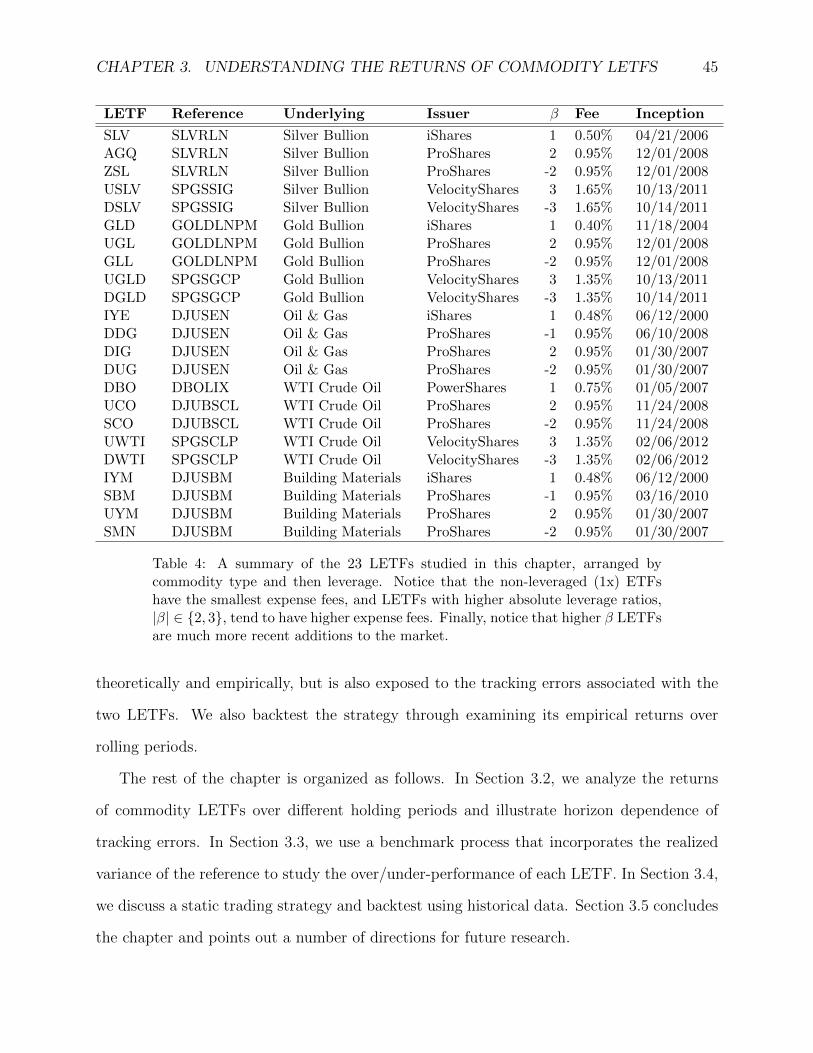
CHAPTER 3. UNDERSTANDING THE RETURNS OF COMMODITY LETFS 45
LETF Reference Underlying Issuer β Fee Inception
SLV SLVRLN Silver Bullion iShares 1 0.50% 04/21/2006AGQ SLVRLN Silver Bullion ProShares 2 0.95% 12/01/2008ZSL SLVRLN Silver Bullion ProShares -2 0.95% 12/01/2008USLV SPGSSIG Silver Bullion VelocityShares 3 1.65% 10/13/2011DSLV SPGSSIG Silver Bullion VelocityShares -3 1.65% 10/14/2011GLD GOLDLNPM Gold Bullion iShares 1 0.40% 11/18/2004UGL GOLDLNPM Gold Bullion ProShares 2 0.95% 12/01/2008GLL GOLDLNPM Gold Bullion ProShares -2 0.95% 12/01/2008UGLD SPGSGCP Gold Bullion VelocityShares 3 1.35% 10/13/2011DGLD SPGSGCP Gold Bullion VelocityShares -3 1.35% 10/14/2011IYE DJUSEN Oil & Gas iShares 1 0.48% 06/12/2000DDG DJUSEN Oil & Gas ProShares -1 0.95% 06/10/2008DIG DJUSEN Oil & Gas ProShares 2 0.95% 01/30/2007DUG DJUSEN Oil & Gas ProShares -2 0.95% 01/30/2007DBO DBOLIX WTI Crude Oil PowerShares 1 0.75% 01/05/2007UCO DJUBSCL WTI Crude Oil ProShares 2 0.95% 11/24/2008SCO DJUBSCL WTI Crude Oil ProShares -2 0.95% 11/24/2008UWTI SPGSCLP WTI Crude Oil VelocityShares 3 1.35% 02/06/2012DWTI SPGSCLP WTI Crude Oil VelocityShares -3 1.35% 02/06/2012IYM DJUSBM Building Materials iShares 1 0.48% 06/12/2000SBM DJUSBM Building Materials ProShares -1 0.95% 03/16/2010UYM DJUSBM Building Materials ProShares 2 0.95% 01/30/2007SMN DJUSBM Building Materials ProShares -2 0.95% 01/30/2007
Table 4: A summary of the 23 LETFs studied in this chapter, arranged bycommodity type and then leverage. Notice that the non-leveraged (1x) ETFshave the smallest expense fees, and LETFs with higher absolute leverage ratios,|β| ∈ 2, 3, tend to have higher expense fees. Finally, notice that higher β LETFsare much more recent additions to the market.
theoretically and empirically, but is also exposed to the tracking errors associated with the
two LETFs. We also backtest the strategy through examining its empirical returns over
rolling periods.
The rest of the chapter is organized as follows. In Section 3.2, we analyze the returns
of commodity LETFs over different holding periods and illustrate horizon dependence of
tracking errors. In Section 3.3, we use a benchmark process that incorporates the realized
variance of the reference to study the over/under-performance of each LETF. In Section 3.4,
we discuss a static trading strategy and backtest using historical data. Section 3.5 concludes
the chapter and points out a number of directions for future research.

CHAPTER 3. UNDERSTANDING THE RETURNS OF COMMODITY LETFS 46
3.2 Analysis of Tracking Error
We first compare the returns of LETFs and their reference indices. For every ETF, we
obtain its closing prices and reference index values from Bloomberg for the period December
2008-May 2013. We then calculate the n-day returns from n = 1, 2, . . . , 30 using disjoint
successive periods (e.g. the return over days 1-30 then returns over days 31-60 for 30-day
returns). Let Lt be the price of an LETF and St be the reference index value at time t. For
a given leverage ratio β, we compare the log-returns of the LETF to β times the log-returns
of the corresponding reference index. This leads us to define the n-day tracking error at time
t by
Y(n)t = ln
Lt+n∆t
Lt− β ln
St+n∆t
St, (3.2.1)
where ∆t represents one trading day. We explore the empirical distribution of the n-day
tracking error, and then analyze the effect of holding horizon on the magnitude of tracking
errors. We remark there are alternative ways to define tracking errors for ETFs. For example,
one can consider the difference in relative returns as opposed to log-returns, or the root mean
square of the daily differences (see Mackintosh and Lin (2010b)).
3.2.1 Regression of Empirical Returns
We conduct a regression between log-returns of the LETF and its reference index based on
the linear model:
lnLtL0
= β lnStS0
+ c+ ε,
where ε ∼ N(0, σ2) is independent of the reference index value St, ∀t ≥ 0. In other words,
we run an ordinary least square 1-variable regression between the log-returns for every fixed
horizon of n days. Then, we increase the holding period from 1 to 30 days, and observe how
the regression coefficients vary.
We display the regression results in Figures 6 through 9 for log-returns over periods of

CHAPTER 3. UNDERSTANDING THE RETURNS OF COMMODITY LETFS 47
1, 5, 10, and 20 days. To avoid dependence among returns, we use disjoint time intervals to
calculate returns. For example, we use S20
S0, S40
S20. . . and L20
L0, L40
L20. . . for 20-day log-returns as
the inputs for the regression.
In Figure 6, the regression coefficient β for DIG (β = 2, oil & gas) increases from 2 to 2.1
as the holding period lengthens from 1 to 20 days. Although the coefficient of determination
R2 is close to 99% for up to 20 days, it is highest for 1-day returns. In Figure 7 for DUG
(β = −2, oil & gas), one again observes β increasing, and R2 decreasing. For DUG (β = −2,
oil & gas), as n varies from 1 to 20, β increases from −2 to −1.66. As a result, this implies
that DIG (β = 2, oil & gas) effectively gains leverage as the holding time increases, while
DUG (β = −2, oil & gas) loses leverage compared to the advertised fund β.
On the other hand, UGL (β = 2, gold) and GLL (β = −2, gold) exhibit very different
return behaviors. In Figure 8 the R2 for UGL (β = 2, gold) is surprisingly worst for the
shortest holding period of 1 day, whereas it increases to 95% over a holding period of 20
days. In Figure 9 for GLL (β = −2, gold), the R2 increases from 35% to 96% when holding
the fund from 1 to 20 days. Furthermore, the estimators β for UGL (β = 2, gold) and GLL
(β = −2, gold) both slowly approach their advertised β = ±2. The variation of β for DIG
(β = 2, oil & gas) and UGL (β = 2, gold) over different holding periods is summarized in
Figure 10.
We observe that LETFs that track an illiquid reference, such as the gold bullion index
GOLDLNPM, tend to have more tracking errors than those tracking a liquid index, such
as the oil & gas index DJUSEN. The oil & gas commodity LETFs involve exchange-traded
futures which are liquid proxy to the spot price. The gold and silver bullion LETFs consist
of OTC total return swaps. The difficulty and higher costs replication using swaps, as well
as infrequent (typically daily) update of the swaps’ mark-to-market values can weaken the
fund’s tracking ability. For example, the 1-day regressions of UGL and GLL (β = ±2, gold)
yield R2 values less than 40%, while DIG and DUG (β = ±2, oil & gas ) have 1-day R2
values of over 90%. On the other hand, full physical replication yields the greatest R2, with
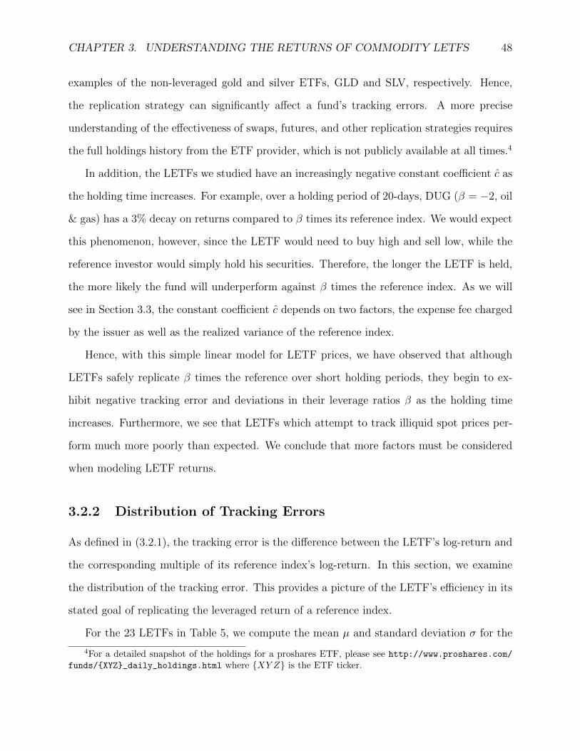
CHAPTER 3. UNDERSTANDING THE RETURNS OF COMMODITY LETFS 48
examples of the non-leveraged gold and silver ETFs, GLD and SLV, respectively. Hence,
the replication strategy can significantly affect a fund’s tracking errors. A more precise
understanding of the effectiveness of swaps, futures, and other replication strategies requires
the full holdings history from the ETF provider, which is not publicly available at all times.4
In addition, the LETFs we studied have an increasingly negative constant coefficient c as
the holding time increases. For example, over a holding period of 20-days, DUG (β = −2, oil
& gas) has a 3% decay on returns compared to β times its reference index. We would expect
this phenomenon, however, since the LETF would need to buy high and sell low, while the
reference investor would simply hold his securities. Therefore, the longer the LETF is held,
the more likely the fund will underperform against β times the reference index. As we will
see in Section 3.3, the constant coefficient c depends on two factors, the expense fee charged
by the issuer as well as the realized variance of the reference index.
Hence, with this simple linear model for LETF prices, we have observed that although
LETFs safely replicate β times the reference over short holding periods, they begin to ex-
hibit negative tracking error and deviations in their leverage ratios β as the holding time
increases. Furthermore, we see that LETFs which attempt to track illiquid spot prices per-
form much more poorly than expected. We conclude that more factors must be considered
when modeling LETF returns.
3.2.2 Distribution of Tracking Errors
As defined in (3.2.1), the tracking error is the difference between the LETF’s log-return and
the corresponding multiple of its reference index’s log-return. In this section, we examine
the distribution of the tracking error. This provides a picture of the LETF’s efficiency in its
stated goal of replicating the leveraged return of a reference index.
For the 23 LETFs in Table 5, we compute the mean µ and standard deviation σ for the
4For a detailed snapshot of the holdings for a proshares ETF, please see http://www.proshares.com/
funds/XYZ_daily_holdings.html where XY Z is the ETF ticker.
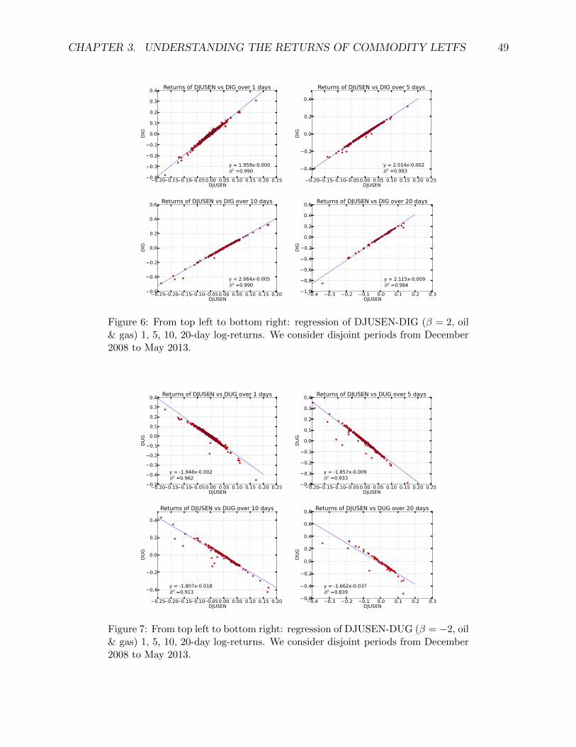
CHAPTER 3. UNDERSTANDING THE RETURNS OF COMMODITY LETFS 49
−0.20−0.15−0.10−0.050.00 0.05 0.10 0.15 0.20 0.25DJUSEN
−0.4
−0.3
−0.2
−0.1
0.0
0.1
0.2
0.3
0.4
DIG
y = 1.959x-0.000R2 =0.990
Returns of DJUSEN vs DIG over 1 days
−0.20−0.15−0.10−0.050.00 0.05 0.10 0.15 0.20 0.25DJUSEN
−0.4
−0.2
0.0
0.2
0.4
DIG
y = 2.014x-0.002R2 =0.993
Returns of DJUSEN vs DIG over 5 days
−0.25−0.20−0.15−0.10−0.050.00 0.05 0.10 0.15 0.20DJUSEN
−0.6
−0.4
−0.2
0.0
0.2
0.4
0.6
DIG
y = 2.064x-0.005R2 =0.990
Returns of DJUSEN vs DIG over 10 days
−0.4 −0.3 −0.2 −0.1 0.0 0.1 0.2 0.3DJUSEN
−1.0
−0.8
−0.6
−0.4
−0.2
0.0
0.2
0.4
0.6
DIG
y = 2.115x-0.009R2 =0.984
Returns of DJUSEN vs DIG over 20 days
Figure 6: From top left to bottom right: regression of DJUSEN-DIG (β = 2, oil& gas) 1, 5, 10, 20-day log-returns. We consider disjoint periods from December2008 to May 2013.
−0.20−0.15−0.10−0.050.00 0.05 0.10 0.15 0.20 0.25DJUSEN
−0.5
−0.4
−0.3
−0.2
−0.1
0.0
0.1
0.2
0.3
0.4
DUG
y = -1.948x-0.002R2 =0.962
Returns of DJUSEN vs DUG over 1 days
−0.20−0.15−0.10−0.050.00 0.05 0.10 0.15 0.20 0.25DJUSEN
−0.4
−0.3
−0.2
−0.1
0.0
0.1
0.2
0.3
0.4
DUG
y = -1.857x-0.009R2 =0.933
Returns of DJUSEN vs DUG over 5 days
−0.25−0.20−0.15−0.10−0.050.00 0.05 0.10 0.15 0.20DJUSEN
−0.4
−0.2
0.0
0.2
0.4
DUG
y = -1.807x-0.018R2 =0.913
Returns of DJUSEN vs DUG over 10 days
−0.4 −0.3 −0.2 −0.1 0.0 0.1 0.2 0.3DJUSEN
−0.6
−0.4
−0.2
0.0
0.2
0.4
0.6
0.8
DUG
y = -1.662x-0.037R2 =0.839
Returns of DJUSEN vs DUG over 20 days
Figure 7: From top left to bottom right: regression of DJUSEN-DUG (β = −2, oil& gas) 1, 5, 10, 20-day log-returns. We consider disjoint periods from December2008 to May 2013.
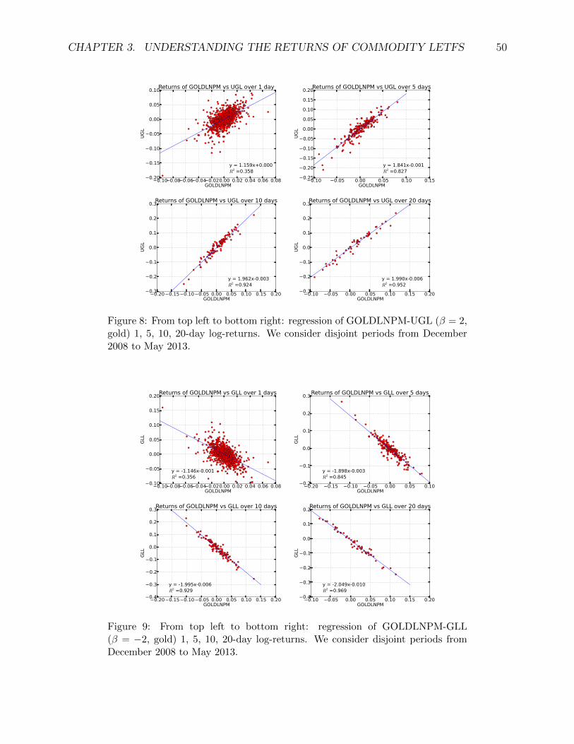
CHAPTER 3. UNDERSTANDING THE RETURNS OF COMMODITY LETFS 50
−0.10−0.08−0.06−0.04−0.020.00 0.02 0.04 0.06 0.08GOLDLNPM
−0.20
−0.15
−0.10
−0.05
0.00
0.05
0.10
UGL
y = 1.159x+0.000R2 =0.358
Returns of GOLDLNPM vs UGL over 1 days
−0.10 −0.05 0.00 0.05 0.10 0.15GOLDLNPM
−0.25
−0.20
−0.15
−0.10
−0.05
0.00
0.05
0.10
0.15
0.20
UGL
y = 1.841x-0.001R2 =0.827
Returns of GOLDLNPM vs UGL over 5 days
−0.20−0.15−0.10−0.05 0.00 0.05 0.10 0.15 0.20GOLDLNPM
−0.3
−0.2
−0.1
0.0
0.1
0.2
0.3
UGL
y = 1.962x-0.003R2 =0.924
Returns of GOLDLNPM vs UGL over 10 days
−0.10 −0.05 0.00 0.05 0.10 0.15 0.20GOLDLNPM
−0.3
−0.2
−0.1
0.0
0.1
0.2
0.3
UGL
y = 1.990x-0.006R2 =0.952
Returns of GOLDLNPM vs UGL over 20 days
Figure 8: From top left to bottom right: regression of GOLDLNPM-UGL (β = 2,gold) 1, 5, 10, 20-day log-returns. We consider disjoint periods from December2008 to May 2013.
−0.10−0.08−0.06−0.04−0.020.00 0.02 0.04 0.06 0.08GOLDLNPM
−0.10
−0.05
0.00
0.05
0.10
0.15
0.20
GLL
y = -1.146x-0.001R2 =0.356
Returns of GOLDLNPM vs GLL over 1 days
−0.20 −0.15 −0.10 −0.05 0.00 0.05 0.10GOLDLNPM
−0.2
−0.1
0.0
0.1
0.2
0.3
GLL
y = -1.898x-0.003R2 =0.845
Returns of GOLDLNPM vs GLL over 5 days
−0.20−0.15−0.10−0.05 0.00 0.05 0.10 0.15 0.20GOLDLNPM
−0.4
−0.3
−0.2
−0.1
0.0
0.1
0.2
0.3
GLL
y = -1.995x-0.006R2 =0.929
Returns of GOLDLNPM vs GLL over 10 days
−0.10 −0.05 0.00 0.05 0.10 0.15 0.20GOLDLNPM
−0.4
−0.3
−0.2
−0.1
0.0
0.1
0.2
GLL
y = -2.049x-0.010R2 =0.969
Returns of GOLDLNPM vs GLL over 20 days
Figure 9: From top left to bottom right: regression of GOLDLNPM-GLL(β = −2, gold) 1, 5, 10, 20-day log-returns. We consider disjoint periods fromDecember 2008 to May 2013.
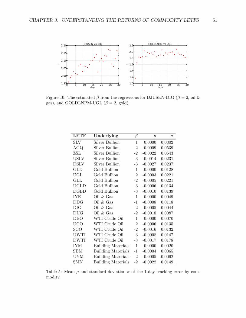
CHAPTER 3. UNDERSTANDING THE RETURNS OF COMMODITY LETFS 51
0 5 10 15 20 25 30days
1.95
2.00
2.05
2.10
2.15
2.20
β
DJUSEN vs DIG
0 5 10 15 20 25 30days
1.0
1.2
1.4
1.6
1.8
2.0
2.2
β
GOLDLNPM vs UGL
Figure 10: The estimated β from the regressions for DJUSEN-DIG (β = 2, oil &gas), and GOLDLNPM-UGL (β = 2, gold).
LETF Underlying β µ σ
SLV Silver Bullion 1 0.0000 0.0302AGQ Silver Bullion 2 -0.0009 0.0539ZSL Silver Bullion -2 -0.0022 0.0543USLV Silver Bullion 3 -0.0014 0.0231DSLV Silver Bullion -3 -0.0027 0.0237GLD Gold Bullion 1 0.0000 0.0128UGL Gold Bullion 2 -0.0003 0.0221GLL Gold Bullion -2 -0.0005 0.0221UGLD Gold Bullion 3 -0.0006 0.0134DGLD Gold Bullion -3 -0.0010 0.0139IYE Oil & Gas 1 0.0000 0.0049DDG Oil & Gas -1 -0.0008 0.0118DIG Oil & Gas 2 -0.0005 0.0044DUG Oil & Gas -2 -0.0018 0.0087DBO WTI Crude Oil 1 0.0000 0.0070UCO WTI Crude Oil 2 -0.0006 0.0135SCO WTI Crude Oil -2 -0.0016 0.0132UWTI WTI Crude Oil 3 -0.0008 0.0147DWTI WTI Crude Oil -3 -0.0017 0.0178IYM Building Materials 1 0.0000 0.0020SBM Building Materials -1 -0.0004 0.0065UYM Building Materials 2 -0.0005 0.0062SMN Building Materials -2 -0.0022 0.0149
Table 5: Mean µ and standard deviation σ of the 1-day tracking error by com-modity.

CHAPTER 3. UNDERSTANDING THE RETURNS OF COMMODITY LETFS 52
−0.05−0.04−0.03−0.02−0.01 0.00 0.01 0.02 0.03Tracking Error
0
50
100
150
200Pr
obab
ility
µ=-0.0005 σ=0.0044
DJUSEN-DIG
−4 −3 −2 −1 0 1 2 3 4Quantiles
−0.05−0.04−0.03−0.02−0.01
0.000.010.020.03
Orde
red
Valu
es
r^2=0.8336
DIG Tracking Error Quantile-Quantile Plot
−0.20 −0.15 −0.10 −0.05 0.00 0.05Tracking Error
0
10
20
30
40
50
60
70
80
Prob
abili
ty
µ=-0.0018 σ=0.0087
DJUSEN-DUG
−4 −3 −2 −1 0 1 2 3 4Quantiles
−0.20
−0.15
−0.10
−0.05
0.00
0.05
Orde
red
Valu
es
r^2=0.5900
DUG Tracking Error Quantile-Quantile Plot
−0.15 −0.10 −0.05 0.00 0.05 0.10 0.15Tracking Error
0
5
10
15
20
25
Prob
abili
ty
µ=-0.0003 σ=0.0221
GOLDLNPM-UGL
−4 −3 −2 −1 0 1 2 3 4Quantiles
−0.15
−0.10
−0.05
0.00
0.05
0.10
0.15
Orde
red
Valu
es
r^2=0.9791
UGL Tracking Error Quantile-Quantile Plot
−0.15 −0.10 −0.05 0.00 0.05 0.10 0.15Tracking Error
0
5
10
15
20
25
Prob
abili
ty
µ=-0.0005 σ=0.0221
GOLDLNPM-GLL
−4 −3 −2 −1 0 1 2 3 4Quantiles
−0.15
−0.10
−0.05
0.00
0.05
0.10
0.15
Orde
red
Valu
es
r^2=0.9778
GLL Tracking Error Quantile-Quantile Plot
Figure 11: Histograms and QQ plots of 1-day tracking errors for DIG, DUG(β = ±2, oil & gas); UGL, GLL (β = ±2, gold) from top to bottom.

CHAPTER 3. UNDERSTANDING THE RETURNS OF COMMODITY LETFS 53
tracking errors using available price data during the period Dec 2008 to May 2013. For all
these funds, the mean 1-day tracking error has µ ≈ 0, ranging from 0% to -0.27%. Therefore,
all these LETFs on average successfully replicate the stated multiple β of the daily reference
return, with a slight negative bias. In fact, many LETFs even continued to replicate returns
over periods as long as 10 days. However, as the holding time increases, the average tracking
error grows more negative, so that the LETF in fact underperforms its intended goal over
longer holding periods (see Figure 11).
Interestingly, the tracking errors for the silver and gold LETFs (AGQ, ZSL (β = ±2,
silver); UGL, GLL (β = ±2, gold)) in Table 5 have σ several magnitudes higher than µ.
For example, AGQ (β = 2, silver) has a tracking error σ of 5% compared to a µ of 0.01%.
In other words, these four LETFs, while they might track their references well on average,
may also exhibit positive and negative deviations over 1-day holding periods as well. These
observations are consistent with the regressions in Figures 8 and 9, where UGL and GLL
(β = ±2, gold) show significant 1-day tracking errors. On the other hand, the non-leveraged
gold and silver bullion ETFs, GLD and SLV, have almost no tracking error σ ≈ 0, because
they hold the underlying bullion according to their prospectuses. Since many investors use
these ETFs to gain leveraged exposure to commodities, they should be aware of the large
variance of the associated tracking errors.
In Figure 11, we show the histogram for the tracking error for each ETF along with a
quantile-quantile plot to illustrate the distribution. For DIG and DUG (β = ±2, oil & gas),
the quantile-quantile plot shows that the tracking error distribution is not quite normal, and
has a large negative tail, so that the commodity LETF tracking error is negatively biased
even for the shortest possible holding period of one day. On the other hand, for UGL, GLL
(β = ±2, gold) the distribution appears to be normal with R2 close to 98%. However, as
noted in Table 5, the tracking errors for UGL and GLL (β = ±2, gold) also have a very large
variance.
Next, we examine the horizon effect of tracking errors. Figure 12 indicates that higher
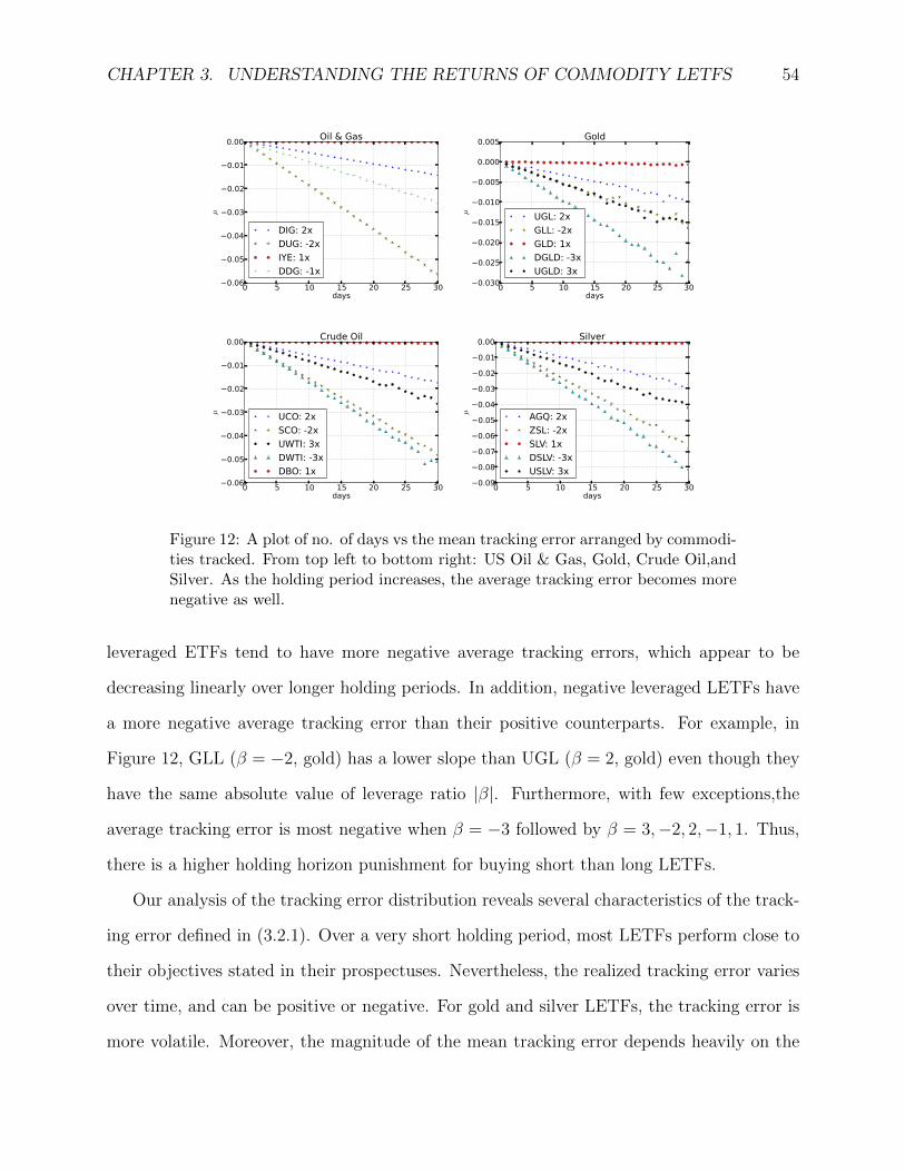
CHAPTER 3. UNDERSTANDING THE RETURNS OF COMMODITY LETFS 54
0 5 10 15 20 25 30days
−0.06
−0.05
−0.04
−0.03
−0.02
−0.01
0.00
µ
Oil & Gas
DIG: 2xDUG: -2xIYE: 1xDDG: -1x
0 5 10 15 20 25 30days
−0.030
−0.025
−0.020
−0.015
−0.010
−0.005
0.000
0.005
µ
Gold
UGL: 2xGLL: -2xGLD: 1xDGLD: -3xUGLD: 3x
0 5 10 15 20 25 30days
−0.06
−0.05
−0.04
−0.03
−0.02
−0.01
0.00
µ
Crude Oil
UCO: 2xSCO: -2xUWTI: 3xDWTI: -3xDBO: 1x
0 5 10 15 20 25 30days
−0.09
−0.08
−0.07
−0.06
−0.05
−0.04
−0.03
−0.02
−0.01
0.00
µ
Silver
AGQ: 2xZSL: -2xSLV: 1xDSLV: -3xUSLV: 3x
Figure 12: A plot of no. of days vs the mean tracking error arranged by commodi-ties tracked. From top left to bottom right: US Oil & Gas, Gold, Crude Oil,andSilver. As the holding period increases, the average tracking error becomes morenegative as well.
leveraged ETFs tend to have more negative average tracking errors, which appear to be
decreasing linearly over longer holding periods. In addition, negative leveraged LETFs have
a more negative average tracking error than their positive counterparts. For example, in
Figure 12, GLL (β = −2, gold) has a lower slope than UGL (β = 2, gold) even though they
have the same absolute value of leverage ratio |β|. Furthermore, with few exceptions,the
average tracking error is most negative when β = −3 followed by β = 3,−2, 2,−1, 1. Thus,
there is a higher holding horizon punishment for buying short than long LETFs.
Our analysis of the tracking error distribution reveals several characteristics of the track-
ing error defined in (3.2.1). Over a very short holding period, most LETFs perform close to
their objectives stated in their prospectuses. Nevertheless, the realized tracking error varies
over time, and can be positive or negative. For gold and silver LETFs, the tracking error is
more volatile. Moreover, the magnitude of the mean tracking error depends heavily on the
CHAPTER 3. UNDERSTANDING THE RETURNS OF COMMODITY LETFS 55
β of the LETF, with bear LETFs suffering a higher penalty than bull LETFs.
3.3 Incorporating Realized Variance into Tracking Er-
ror Measurement
As is well known in the industry (see Avellaneda and Zhang (2010); Cheng and Madhavan
(2009)), the price dynamics of an LETF depends on the realized variance of the reference
index. This leads us to incorporate the realized variance in measuring the performance of
an LETF. We run a regression analysis based on empirical LETF and reference prices that
incorporates the realized variance as an independent variable. We then derive a realized
effective fee associated with each LETF and analyze the realized price behavior relative to a
theoretical benchmark to better quantify the over/under-performance.
3.3.1 Model for the LETF Price
Let St be the price of the reference index, and Lt be the price of the LETF at time t. Also
denote f as the expense rate, r as the interest rate and β as the leverage ratio. Assume the
reference asset follows the SDE
dStSt
= µtdt+ σtdWt, t ≥ 0, (3.3.1)
with stochastic drift (µt)t≥0 and volatility (σt)t≥0. For our analysis herein, we assume a
general diffusion framework, but do not need to specify a parametric model. Many well-
known models, including the CEV, Heston, and exponential Ornstein-Uhlenbeck models, fit
within the above framework.
A long β-LETF L can be constructed through a dynamic portfolio. Specifically, the
portfolio at time t consists of the cash amount $βLt invested in the reference index St, while
$(β − 1)Lt is borrowed at the positive risk free rate r. As a result, the LETF satisfies the
CHAPTER 3. UNDERSTANDING THE RETURNS OF COMMODITY LETFS 56
SDE
dLt = LtβdStSt− Lt((β − 1)r + f)dt.
Solving the SDE, the log-return of the LETF is given by
lnLtL0
= β lnStS0
+β − β2
2Vt + ((1− β)r − f)t, (3.3.2)
where
Vt =
∫ t
0
σ2sds
is the realized variance of S accumulated up to time t. Therefore, under this general diffusion
model, the log-return of the LETF is proportional to the log-return of the reference index by
a factor of β, but also proportional to the variance by a factor of β−β2
2. The latter factor is
negative if β /∈ (0, 1), which is true for every LETF traded on the market. Also, the expense
fee f reduces the return of the LETF.
Our regression analysis will focus on testing the functional form (3.3.2). We observe from
(3.3.2) that the functional form of Lt in terms of St and Vt holds for any parametric model
within the diffusion framework in (3.3.1). Considering the daily LETF returns, we set
∆t = 1252
as one trading day. Let RSt be the daily return of the reference index at time t. At
any time t, the n-day log-returns of an LETF follows
lnLt+n∆t
Lt= β ln
St+n∆t
St+β − β2
2V
(n)t + ((1− β)r − f)n∆t, (3.3.3)
V(n)t =
n−1∑i=0
(RSt+i∆t − Rt
S)2, Rt
S=
1
n
n−1∑i=0
RSt+i∆t.
This serves as a benchmark process for our subsequent analysis.
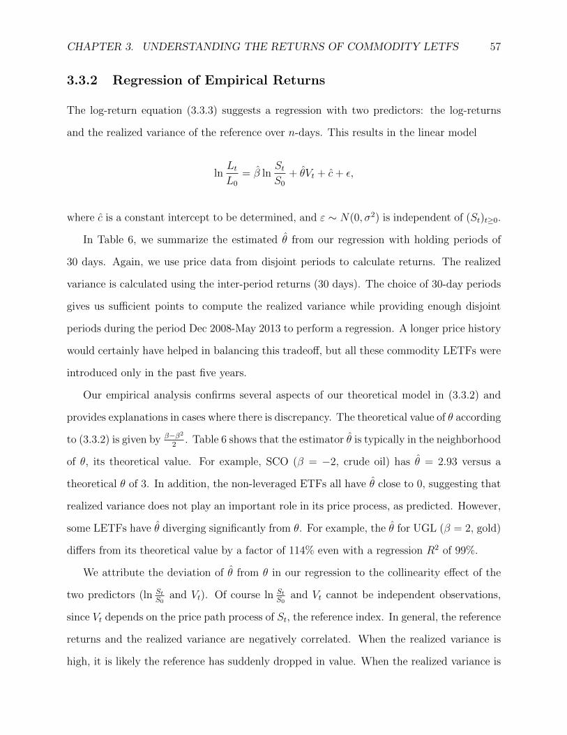
CHAPTER 3. UNDERSTANDING THE RETURNS OF COMMODITY LETFS 57
3.3.2 Regression of Empirical Returns
The log-return equation (3.3.3) suggests a regression with two predictors: the log-returns
and the realized variance of the reference over n-days. This results in the linear model
lnLtL0
= β lnStS0
+ θVt + c+ ε,
where c is a constant intercept to be determined, and ε ∼ N(0, σ2) is independent of (St)t≥0.
In Table 6, we summarize the estimated θ from our regression with holding periods of
30 days. Again, we use price data from disjoint periods to calculate returns. The realized
variance is calculated using the inter-period returns (30 days). The choice of 30-day periods
gives us sufficient points to compute the realized variance while providing enough disjoint
periods during the period Dec 2008-May 2013 to perform a regression. A longer price history
would certainly have helped in balancing this tradeoff, but all these commodity LETFs were
introduced only in the past five years.
Our empirical analysis confirms several aspects of our theoretical model in (3.3.2) and
provides explanations in cases where there is discrepancy. The theoretical value of θ according
to (3.3.2) is given by β−β2
2. Table 6 shows that the estimator θ is typically in the neighborhood
of θ, its theoretical value. For example, SCO (β = −2, crude oil) has θ = 2.93 versus a
theoretical θ of 3. In addition, the non-leveraged ETFs all have θ close to 0, suggesting that
realized variance does not play an important role in its price process, as predicted. However,
some LETFs have θ diverging significantly from θ. For example, the θ for UGL (β = 2, gold)
differs from its theoretical value by a factor of 114% even with a regression R2 of 99%.
We attribute the deviation of θ from θ in our regression to the collinearity effect of the
two predictors (ln StS0
and Vt). Of course ln StS0
and Vt cannot be independent observations,
since Vt depends on the price path process of St, the reference index. In general, the reference
returns and the realized variance are negatively correlated. When the realized variance is
high, it is likely the reference has suddenly dropped in value. When the realized variance is
CHAPTER 3. UNDERSTANDING THE RETURNS OF COMMODITY LETFS 58
LETF Underlying β θ θ r2 r2x|y r2
y|x
SLV Silver Bullion 1 0.11 0 0.9799 0.9503 0.0078AGQ Silver Bullion 2 -1.31 -1 0.9885 0.9751 0.3892ZSL Silver Bullion -2 -3.27 -3 0.9995 0.9988 0.7514USLV Silver Bullion 3 -2.24 -3 0.9995 0.9988 0.7514DSLV Silver Bullion -3 -6.94 -6 0.9994 0.9989 0.9654GLD Gold Bullion 1 -0.14 0 0.9898 0.9791 0.0064UGL Gold Bullion 2 -2.44 -1 0.9934 0.9867 0.2900GLL Gold Bullion -2 -0.96 -3 0.9914 0.9828 0.0417UGLD Gold Bullion 3 -2.38 -3 0.9982 0.9955 0.6355DGLD Gold Bullion -3 -6.26 -6 0.9846 0.9685 0.0809IYE Oil & Gas 1 -0.06 0 0.9988 0.9965 0.1905DDG Oil & Gas -1 -0.99 -1 0.8866 0.7662 0.2342DIG Oil & Gas 2 -1.11 -1 0.9996 0.9989 0.9498DUG Oil & Gas -2 -3.31 -3 0.9884 0.9769 0.8873DBO WTI Crude Oil 1 -0.02 0 0.9992 0.9981 0.0035UCO WTI Crude Oil 2 -1.15 -1 0.9987 0.9972 0.7747SCO WTI Crude Oil -2 -2.93 -3 0.9987 0.9975 0.9619UWTI WTI Crude Oil 3 -2.14 -3 0.9974 0.9939 0.6218DWTI WTI Crude Oil -3 -7.25 -6 0.9974 0.9939 0.6218IYM Building Materials 1 0.03 0 0.9996 0.9987 0.0495SBM Building Materials -1 -0.98 -1 0.9970 0.9920 0.5446UYM Building Materials 2 -1.10 -1 0.9997 0.9993 0.9380SMN Building Materials -2 -3.59 -3 0.9613 0.9221 0.5301
Table 6: θ vs. θ, estimated from 30-day multi-variable regression of returns, witha partial correlation table. r2
y|x stands for the marginal predictive power of adding
the realized variance (y) into the model, holding constant the predictive powerof the reference index returns (x). Similar definition for r2
x|y. Data from Dec2008-May 2013.
CHAPTER 3. UNDERSTANDING THE RETURNS OF COMMODITY LETFS 59
low, it usually implies a period of steady positive growth for the reference. Thus, the multi-
collinearity effect is responsible for shifting predictive power among the different predictor
variables. In order to measure the magnitude of the collinearity effect and the contribution
of each correlated predictor variable, we compute the coefficients of partial determination
for our regression model.
The factor r2y|x which measures the marginal predictive power of adding the realized vari-
ance into the model. As r2y|x increases, θ becomes closer to θ, suggesting a larger dependence
of LETF returns on realized variance during holding periods of high volatility. For example,
for the 3 LETFs DIG (β = 2, oil & gas), SCO (β = −2, crude oil), and UYM (β = 2,
building materials) all have r2y|x over 90%. Their estimated θ is similarly very close to the
theoretical θ, never differing by more than 10%. However, for non-leveraged ETFs, the real-
ized variance has minimal added predictive power in the model. For those ETFs, we observe
θ ≈ 0. For example, SLV (β = 1, silver), GLD (β = 1, gold), and DBO (β = 1, crude oil)
all have r2y|x ≈ 0, and they subsequently have θ ≈ 0. In addition, r2
x|y, which is the marginal
predictive power of adding the log-returns of the reference into our regression model, is al-
ways very high, indicating that the log-returns of the reference affect the LETF prices the
most, but that the realized variance is still important for predictive power, especially when
leverage and the holding period is high.
3.3.3 Realized Effective Fee
In Figure 13, we show three empirical price paths: the LETF log-returns, the benchmark
process defined in (3.3.2), and β times the reference index log-returns. As we can see, the
value erosion due to realized variance (volatility decay) starts to play a significant role in
determining LETF prices as the holding time increases. The path associated with β times
the reference log-returns dominates the LETF log-returns after about 1 month of holding.
After about 1 year, the benchmark which incorporates volatility decay more closely models
the empirical LETF log-returns. For example, after 6 months of holding, SCO (β = −2,
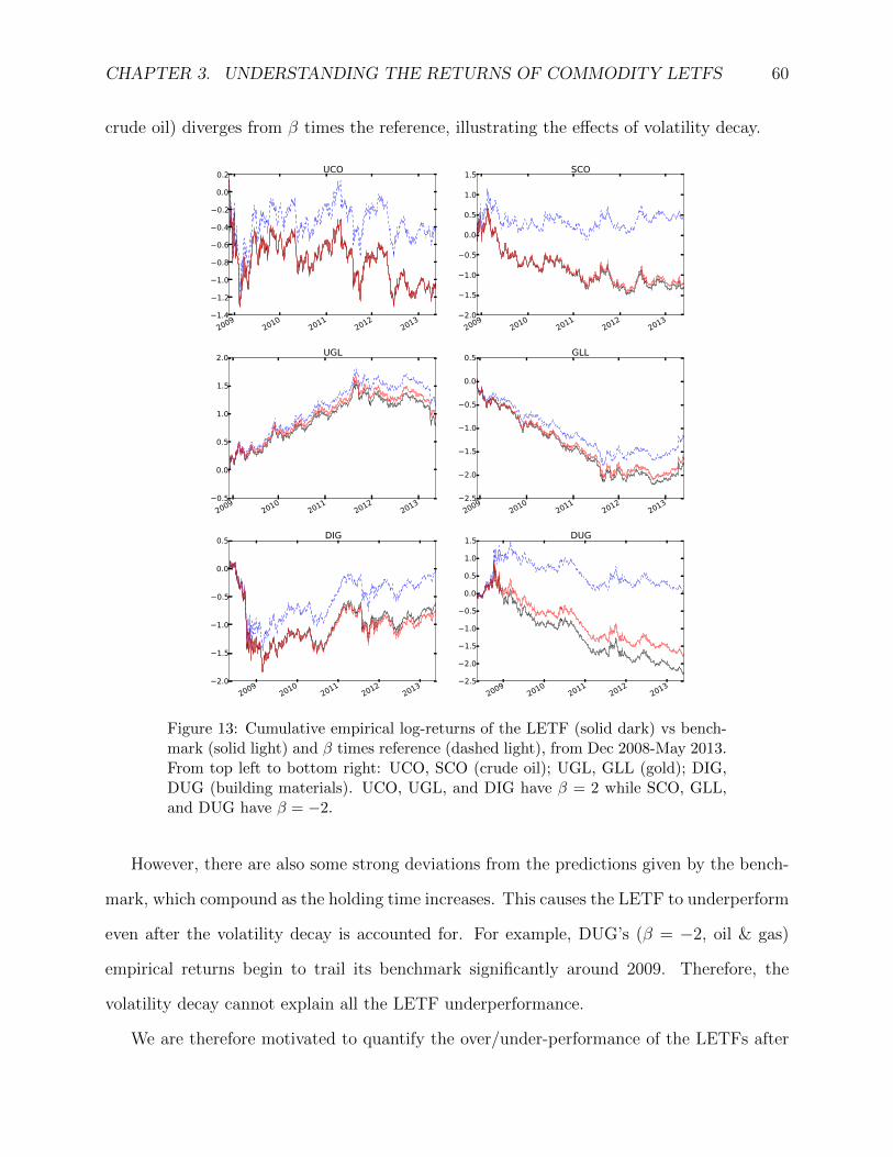
CHAPTER 3. UNDERSTANDING THE RETURNS OF COMMODITY LETFS 60
crude oil) diverges from β times the reference, illustrating the effects of volatility decay.
2009
2010
2011
2012
2013−1.4
−1.2
−1.0
−0.8
−0.6
−0.4
−0.2
0.0
0.2 UCO
2009
2010
2011
2012
2013−2.0
−1.5
−1.0
−0.5
0.0
0.5
1.0
1.5 SCO
2009
2010
2011
2012
2013−0.5
0.0
0.5
1.0
1.5
2.0 UGL
2009
2010
2011
2012
2013−2.5
−2.0
−1.5
−1.0
−0.5
0.0
0.5 GLL
2009
2010
2011
2012
2013−2.0
−1.5
−1.0
−0.5
0.0
0.5 DIG
2009
2010
2011
2012
2013−2.5
−2.0
−1.5
−1.0
−0.5
0.0
0.5
1.0
1.5 DUG
Figure 13: Cumulative empirical log-returns of the LETF (solid dark) vs bench-mark (solid light) and β times reference (dashed light), from Dec 2008-May 2013.From top left to bottom right: UCO, SCO (crude oil); UGL, GLL (gold); DIG,DUG (building materials). UCO, UGL, and DIG have β = 2 while SCO, GLL,and DUG have β = −2.
However, there are also some strong deviations from the predictions given by the bench-
mark, which compound as the holding time increases. This causes the LETF to underperform
even after the volatility decay is accounted for. For example, DUG’s (β = −2, oil & gas)
empirical returns begin to trail its benchmark significantly around 2009. Therefore, the
volatility decay cannot explain all the LETF underperformance.
We are therefore motivated to quantify the over/under-performance of the LETFs after

CHAPTER 3. UNDERSTANDING THE RETURNS OF COMMODITY LETFS 61
observing deviations from the benchmark in Figure 13. We introduce the concept of realized
effective fee (REF) as the effective deduction rate charged by the LETF provider over the
frictionless dynamic portfolio from which the LETF is constructed in Section 3.3.1. For a
holding interval [0, t], the corresponding REF is defined by
ft = (1− β)r −ln Lt
L0− β ln St
S0− β−β2
2Vt
t. (3.3.4)
Since for each LETF, Lt, St, Vt, β, and r are all known, we can calculate the REF ft for any
LETF over a given holding period [0, t] using historical prices. We remark that the REF,
which is indexed by time t, depends on the selected holding horizon.
LETF Underlying β Prospectus Fee (bps) Realized Effective Fee (bps)
SLV Silver Bullion 1 50 96AGQ Silver Bullion 2 95 524ZSL Silver Bullion -2 95 567USLV Silver Bullion 3 165 93DSLV Silver Bullion -3 165 504GLD Gold Bullion 1 40 48UGL Gold Bullion 2 95 343GLL Gold Bullion -2 95 406UGLD Gold Bullion 3 135 139DGLD Gold Bullion -3 135 521IYE Oil & Gas 1 48 50DDG Oil & Gas -1 95 953DIG Oil & Gas 2 95 -142DUG Oil & Gas 2 95 1134DBO WTI Crude Oil 1 75 56UCO WTI Crude Oil 2 95 84SCO WTI Crude Oil -2 95 321UWTI WTI Crude Oil 3 135 3DWTI WTI Crude Oil -3 135 549IYM Building Materials 1 48 11SBM Building Materials -1 95 456UYM Building Materials 2 95 -204SMN Building Materials -2 95 1625
Table 7: Comparison of the official fee for the LETF charged on the fund prospec-tus and the REF calculated using 5 years of price data (December 2008-May 2013)for the LETF and reference (see (3.3.4)). We set r = 69.1 bps, the annualizedLIBOR rate.

CHAPTER 3. UNDERSTANDING THE RETURNS OF COMMODITY LETFS 62
In many cases, the REF is seen to be much larger than the fund’s advertised fee, indicating
significant underperformance. Out of the 23 commodity LETFs, 2 have negative implied
costs, so that the fund overperforms by the end of the five year period Dec 2008 to May
2013. If the REF exceeds the advertised fee, then the investor effectively pays an extra price
for the opportunity to invest in the LETF. As a general trend, the bear LETFs tend to charge
higher REFs than bull LETFs with the same magnitude of leverage |β|. For example, USLV
(β = 2, silver) has a REF of 93 bps, while DSLV (β = −2, silver) has an REF of 504 bps
over the period Dec 2008-May 2013. The two highest REFs correspond to DUG (β = −2,
oil & gas) and SMN (β = −2, building materials), whose REFs are 1134 bps and 1625 bps
respectively. Figure 13 illustrates that DUG (β = −2, oil & gas) drastically underperforms
the benchmark, thereby realizing a high REF. Notice that in both cases, however, DUG
and SMN’s bull counterparts DIG (β = 2, oil & gas) and UYM (β = 2, building materials)
respectively)display a negative REF, indicating overperformance during the same period. It
is possible that as the reference trends upwards for a long period of time, the bear LETF
will underperform, while the bull LETF will overperform.
3.4 A Static LETF Portfolio
Taking advantage of the volatility decay, a well-known trading strategy used by practitioners
involves shorting a ±β pair of LETFs with the same reference, as discussed in Avellaneda and
Zhang (2010); Leung and Santoli (2013); Mackintosh and Lin (2010a); Mason et al. (2010).
Since the LETFs have opposite daily returns on the same reference index, the portfolio has
very little exposure to the reference as long as the holding period is sufficiently short. With
this strategy, the volatility decay can help generate profit, which is the intuition of many
practitioners. However, the portfolio is exposed to risk during periods of low volatility and
high trending, as well as tracking errors. In this section, we describe an extension of this
trading strategy by allowing the positive and negative leverage ratios to differ. We determine
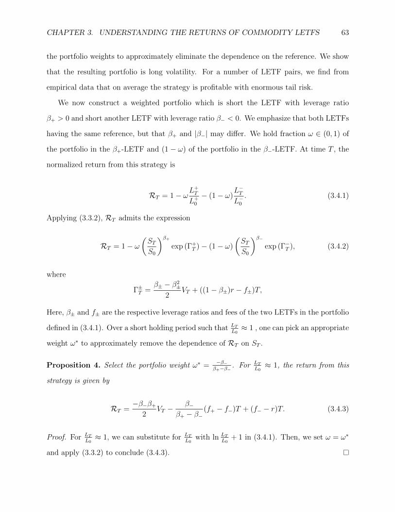
CHAPTER 3. UNDERSTANDING THE RETURNS OF COMMODITY LETFS 63
the portfolio weights to approximately eliminate the dependence on the reference. We show
that the resulting portfolio is long volatility. For a number of LETF pairs, we find from
empirical data that on average the strategy is profitable with enormous tail risk.
We now construct a weighted portfolio which is short the LETF with leverage ratio
β+ > 0 and short another LETF with leverage ratio β− < 0. We emphasize that both LETFs
having the same reference, but that β+ and |β−| may differ. We hold fraction ω ∈ (0, 1) of
the portfolio in the β+-LETF and (1 − ω) of the portfolio in the β−-LETF. At time T , the
normalized return from this strategy is
RT = 1− ωL+T
L+0
− (1− ω)L−TL−0
. (3.4.1)
Applying (3.3.2), RT admits the expression
RT = 1− ω(STS0
)β+exp (Γ+
T )− (1− ω)
(STS0
)β−exp (Γ−T ), (3.4.2)
where
Γ±T =β± − β2
±
2VT + ((1− β±)r − f±)T,
Here, β± and f± are the respective leverage ratios and fees of the two LETFs in the portfolio
defined in (3.4.1). Over a short holding period such that LTL0≈ 1 , one can pick an appropriate
weight ω∗ to approximately remove the dependence of RT on ST .
Proposition 4. Select the portfolio weight ω∗ = −β−β+−β− . For LT
L0≈ 1, the return from this
strategy is given by
RT =−β−β+
2VT −
β−β+ − β−
(f+ − f−)T + (f− − r)T. (3.4.3)
Proof. For LTL0≈ 1, we can substitute for LT
L0with ln LT
L0+ 1 in (3.4.1). Then, we set ω = ω∗
and apply (3.3.2) to conclude (3.4.3).

CHAPTER 3. UNDERSTANDING THE RETURNS OF COMMODITY LETFS 64
(β+, β−) ω∗ −β−β+2
(1,−1) 1/2 1/2(1,−2) 2/3 1(1,−3) 3/4 3/2(2,−1) 1/3 1(2,−2) 1/2 2(2,−3) 3/5 3(3,−1) 1/4 3/2(3,−2) 2/5 3(3,−3) 1/2 9/2
Table 8: Table of (β+, β−) pairs vs ω∗ the weight of the β+ portfolio, and −β−β+2the dependence of the strategy on Vt (see Prop. 4).
The return (3.4.3) corresponding to portfolio weight ω∗ reflects a linear dependence on
the realized variance. In particular, the coefficient −β−β+2
is strictly positive, so the strategy
is effectively long volatility (VT ). Also, as it does not depend on ST , the ω∗ portfolio is
∆-neutral as long as the reference does not move significantly. In Table 8, we summarize the
coefficient of VT and the weighted portfolio (ω∗, 1−ω∗) for different combinations of leverage
ratios. Note that as long as β+ = −β−, we end up with the portfolio weight ω∗ = 12. Also,
the coefficient −β−β+2
exceeds or equals to 1 except for the pair (β+, β−) = (1,−1), and it is
largest for the pair (β+, β−) = (3,−3).
We now backtest the ω∗ strategy from Prop. 4 as follows. For each LETF pair, we short
$0.5 of the β+-LETF and $0.5 of the β−-LETF with β+ = −β− = 2 and hold the position for
some time T . The normalized return RT depends on the relative weights on the long/short-
LETFs but not the absolute cash amounts. More generally, one can also test the strategy
with different β± and ω∗.
Dividing the price data from Dec 2008-May 2013 into n-day rolling (overlapping) periods,
we calculate the returns from the strategy over each period. For every n-day return, we
compare against the realized variance over the same period. This is illustrated in Figure
14. As a theoretical benchmark, we also plot RT in (3.4.3) as a linear function. Each
point (dot) on the plots represents a 5-day return, but over rolling periods the returns are
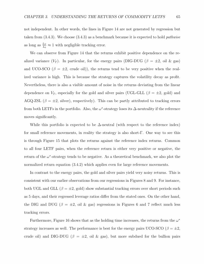
CHAPTER 3. UNDERSTANDING THE RETURNS OF COMMODITY LETFS 65
not independent. In other words, the lines in Figure 14 are not generated by regression but
taken from (3.4.3). We choose (3.4.3) as a benchmark because it is expected to hold pathwise
as long as LTL0≈ 1 with negligible tracking error.
We can observe from Figure 14 that the returns exhibit positive dependence on the re-
alized variance (VT ). In particular, for the energy pairs (DIG-DUG (β = ±2, oil & gas)
and UCO-SCO (β = ±2, crude oil)), the returns tend to be very positive when the real-
ized variance is high. This is because the strategy captures the volatility decay as profit.
Nevertheless, there is also a visible amount of noise in the returns deviating from the linear
dependence on VT , especially for the gold and silver pairs (UGL-GLL (β = ±2, gold) and
AGQ-ZSL (β = ±2, silver), respectively). This can be partly attributed to tracking errors
from both LETFs in the portfolio. Also, the ω∗-strategy loses its ∆-neutrality if the reference
moves significantly.
While this portfolio is expected to be ∆-neutral (with respect to the reference index)
for small reference movements, in reality the strategy is also short-Γ. One way to see this
is through Figure 15 that plots the returns against the reference index returns. Common
to all four LETF pairs, when the reference return is either very positive or negative, the
return of the ω∗-strategy tends to be negative. As a theoretical benchmark, we also plot the
normalized return equation (3.4.2) which applies even for large reference movements.
In contrast to the energy pairs, the gold and silver pairs yield very noisy returns. This is
consistent with our earlier observations from our regressions in Figures 8 and 9. For instance,
both UGL and GLL (β = ±2, gold) show substantial tracking errors over short periods such
as 5 days, and their regressed leverage ratios differ from the stated ones. On the other hand,
the DIG and DUG (β = ±2, oil & gas) regressions in Figures 6 and 7 reflect much less
tracking errors.
Furthermore, Figure 16 shows that as the holding time increases, the returns from the ω∗
strategy increases as well. The performance is best for the energy pairs UCO-SCO (β = ±2,
crude oil) and DIG-DUG (β = ±2, oil & gas), but more subdued for the bullion pairs

CHAPTER 3. UNDERSTANDING THE RETURNS OF COMMODITY LETFS 66
0.00 0.01 0.02 0.03 0.04 0.05 0.06 0.07 0.08 0.09Realized Variance Vt
−0.10
−0.05
0.00
0.05
0.10
0.15
0.20
Retu
rns
(a) DJUSEN-DIG-DUG
0.000 0.001 0.002 0.003 0.004 0.005 0.006 0.007 0.008Realized Variance Vt
−0.10
−0.05
0.00
0.05
0.10
0.15
Retu
rns
(b) GOLDLNPM-UGL-GLL
0.000 0.005 0.010 0.015 0.020 0.025 0.030 0.035 0.040Realized Variance Vt
−0.10
−0.08
−0.06
−0.04
−0.02
0.00
0.02
0.04
0.06
0.08
Retu
rns
(c) DJUBSCL-UCO-SCO
0.00 0.01 0.02 0.03 0.04 0.05 0.06 0.07 0.08 0.09Realized Variance Vt
−0.3
−0.2
−0.1
0.0
0.1
0.2
0.3
Retu
rns
(d) SLVRLN-AGQ-ZSL
Figure 14: Plot of trading returns vs realized variance for a double short strategyover 5-day rolling holding periods, with β± = ±2 for each LETF pair. We com-pare with the empirical returns (circle) from the ω∗ strategy with the predictedreturn (solid line) in Prop. 4. Trading pairs are DIG-DUG (oil & gas), UGL-GLL(gold), UCO-SCO (crude oil), AGQ-ZSL (silver).
UGL-GLL (β = ±2, gold) and AGQ-ZSL (β = ±2, silver). However, over longer holding
periods, the ω∗ portfolio may lose its ∆-neutral status, thereby generating more risk as well.
Although average returns from the ω∗ strategy are positive, one is subject to enormous tail
risk, which increases with the holding time of the static portfolio. In order to ensure that
we do not subject ourselves to excessive tail risk, we should not only be sure of a high
volatility environment, but we must also adjust the holding time to account for the extra
risk associated with time horizon of returns.
Figure 17 gives another perspective of the ω∗ strategy’s dependence on realized variance.
It shows the time series of the 30-day rolling returns along with the realized variance of
the reference index from Dec 2008 to May 2013. We see that when the realized variance
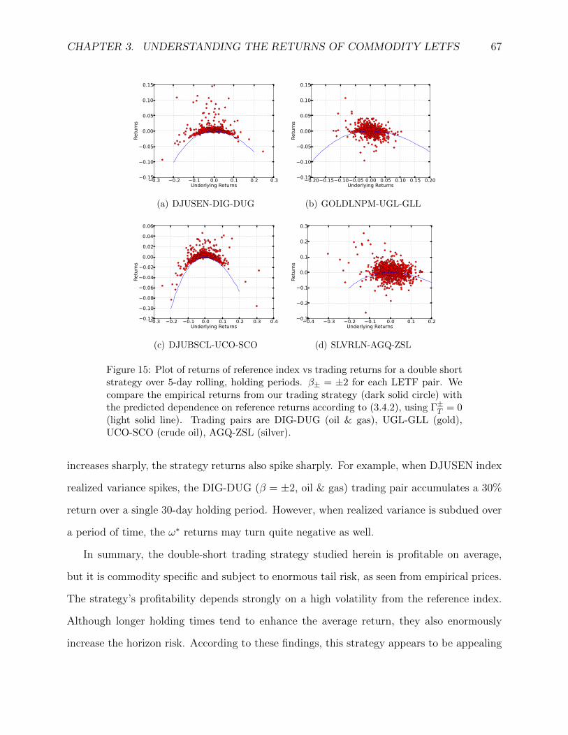
CHAPTER 3. UNDERSTANDING THE RETURNS OF COMMODITY LETFS 67
−0.3 −0.2 −0.1 0.0 0.1 0.2 0.3Underlying Returns
−0.15
−0.10
−0.05
0.00
0.05
0.10
0.15
Retu
rns
(a) DJUSEN-DIG-DUG
−0.20−0.15−0.10−0.05 0.00 0.05 0.10 0.15 0.20Underlying Returns
−0.15
−0.10
−0.05
0.00
0.05
0.10
0.15
Retu
rns
(b) GOLDLNPM-UGL-GLL
−0.3 −0.2 −0.1 0.0 0.1 0.2 0.3 0.4Underlying Returns
−0.12
−0.10
−0.08
−0.06
−0.04
−0.02
0.00
0.02
0.04
0.06
Retu
rns
(c) DJUBSCL-UCO-SCO
−0.4 −0.3 −0.2 −0.1 0.0 0.1 0.2Underlying Returns
−0.3
−0.2
−0.1
0.0
0.1
0.2
0.3
Retu
rns
(d) SLVRLN-AGQ-ZSL
Figure 15: Plot of returns of reference index vs trading returns for a double shortstrategy over 5-day rolling, holding periods. β± = ±2 for each LETF pair. Wecompare the empirical returns from our trading strategy (dark solid circle) withthe predicted dependence on reference returns according to (3.4.2), using Γ±T = 0(light solid line). Trading pairs are DIG-DUG (oil & gas), UGL-GLL (gold),UCO-SCO (crude oil), AGQ-ZSL (silver).
increases sharply, the strategy returns also spike sharply. For example, when DJUSEN index
realized variance spikes, the DIG-DUG (β = ±2, oil & gas) trading pair accumulates a 30%
return over a single 30-day holding period. However, when realized variance is subdued over
a period of time, the ω∗ returns may turn quite negative as well.
In summary, the double-short trading strategy studied herein is profitable on average,
but it is commodity specific and subject to enormous tail risk, as seen from empirical prices.
The strategy’s profitability depends strongly on a high volatility from the reference index.
Although longer holding times tend to enhance the average return, they also enormously
increase the horizon risk. According to these findings, this strategy appears to be appealing
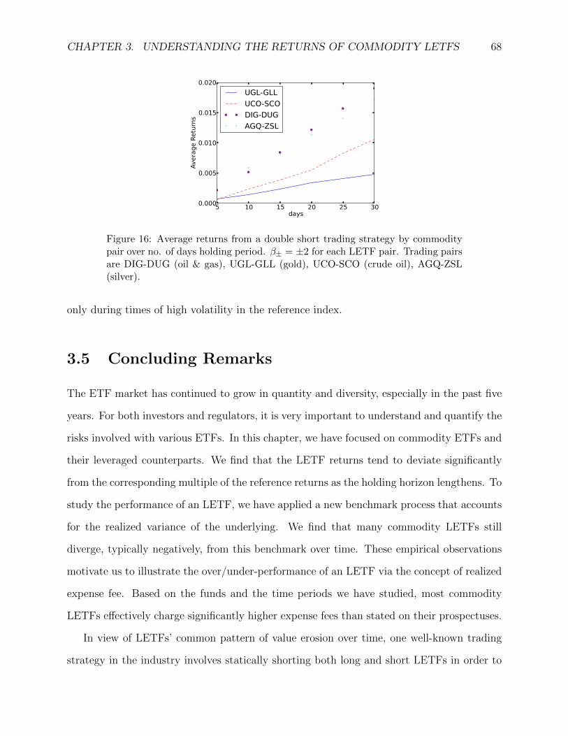
CHAPTER 3. UNDERSTANDING THE RETURNS OF COMMODITY LETFS 68
5 10 15 20 25 30days
0.000
0.005
0.010
0.015
0.020
Averag
e Re
turns
UGL-GLLUCO-SCODIG-DUGAGQ-ZSL
Figure 16: Average returns from a double short trading strategy by commoditypair over no. of days holding period. β± = ±2 for each LETF pair. Trading pairsare DIG-DUG (oil & gas), UGL-GLL (gold), UCO-SCO (crude oil), AGQ-ZSL(silver).
only during times of high volatility in the reference index.
3.5 Concluding Remarks
The ETF market has continued to grow in quantity and diversity, especially in the past five
years. For both investors and regulators, it is very important to understand and quantify the
risks involved with various ETFs. In this chapter, we have focused on commodity ETFs and
their leveraged counterparts. We find that the LETF returns tend to deviate significantly
from the corresponding multiple of the reference returns as the holding horizon lengthens. To
study the performance of an LETF, we have applied a new benchmark process that accounts
for the realized variance of the underlying. We find that many commodity LETFs still
diverge, typically negatively, from this benchmark over time. These empirical observations
motivate us to illustrate the over/under-performance of an LETF via the concept of realized
expense fee. Based on the funds and the time periods we have studied, most commodity
LETFs effectively charge significantly higher expense fees than stated on their prospectuses.
In view of LETFs’ common pattern of value erosion over time, one well-known trading
strategy in the industry involves statically shorting both long and short LETFs in order to

CHAPTER 3. UNDERSTANDING THE RETURNS OF COMMODITY LETFS 69
20092010
20112012
2013−0.3
−0.2
−0.1
0.0
0.1
0.2
0.3
0.4
Retu
rns
0.00
0.02
0.04
0.06
0.08
0.10
0.12
0.14
0.16
0.18
Vt
Returns 30 day: DIG-DUG
20092010
20112012
2013−0.10
−0.08
−0.06
−0.04
−0.02
0.00
0.02
0.04
0.06
0.08
Retu
rns
0.000
0.002
0.004
0.006
0.008
0.010
0.012
0.014
0.016
0.018
Vt
Returns 30 day: UGL-GLL
20092010
20112012
2013−0.4
−0.3
−0.2
−0.1
0.0
0.1
0.2
Retu
rns
0.00
0.02
0.04
0.06
0.08
0.10
0.12
Vt
Returns 30 day: UCO-SCO
20092010
20112012
2013−0.3
−0.2
−0.1
0.0
0.1
0.2
0.3
Retu
rns
0.00
0.02
0.04
0.06
0.08
0.10
0.12
Vt
Returns 30 day: AGQ-ZSL
Figure 17: Time series of returns for a double short strategy over 30-day rolling,holding periods, with β± = ±2 for each LETF pair. Notice how during theperiods of greatest volatility the double short strategy has the greatest return.Trading pairs are DIG-DUG (oil & gas), UGL-GLL (gold), UCO-SCO (crude oil),AGQ-ZSL (silver).
CHAPTER 3. UNDERSTANDING THE RETURNS OF COMMODITY LETFS 70
capture the volatility decay as profit. We systematically study an extension of this strategy
that is applicable to LETF pairs with different asymmetric leverage ratios. We analytically
derive the specific weights in the LETFs so that the resulting portfolio is approximately ∆-
neutral, but short-Γ as well. This strategy can potentially be quite profitable but its return
can be negatively impacted by tracking errors generated by the LETFs and large movements
of the reference index. These two factors both depend on the holding horizon. This should
motivate future research on the horizon risk for LETF strategies. To this end, Leung and
Santoli Leung and Santoli (2013) study the admissible holding horizon and leverage ratio
given a risk constraint. The recent chapters Leung and Li (2015); Naylor et al. (2011);
Triantafyllopoulos and Montana (2009) examine the dynamics of price spreads between ETF
pairs, for example, gold vs. silver.
Our analysis herein does not assume a parametric stochastic volatility model for the
underlying. It is of practical interest to investigate the price behavior of LETF under a
number of well-known stochastic volatility models, such as the Heston and SABR models.
On top of LETFs, there are also options written on these funds. This gives rise to the
question of consistent pricing of LETF options across leverage ratios (see Ahn et al. (2012);
Leung and Sircar (2012)). Finally, models that capture the connection between LETFs and
the broader financial market would be very useful for not only traders and investors, but
also regulators.
Chapter 4
Non-convergence of Agricultural
Futures
This chapter studies the market phenomenon of non-convergence between futures and spot
prices in the grains market. We postulate that the positive basis observed at maturity stems
from the futures holder’s timing options to exercise the shipping certificate delivery item
and subsequently liquidate the physical grain. In our proposed approach, we incorporate
stochastic spot price and storage cost, and solve an optimal double stopping problem to give
the optimal strategies to exercise and liquidate the grain. Our new models for stochastic
storage rates lead to explicit no-arbitrage prices for the shipping certificate and associated
futures contract. We calibrate our models to empirical futures data during the periods of
observed non-convergence, and illustrate the premium generated by the shipping certificate.
4.1 Introduction
Standard no-arbitrage pricing theory asserts that spot and futures prices must converge at
expiration. Nevertheless, during 2004-2009 traders observed significantly higher expiring
futures prices for corn, wheat, and soybeans on the CBOT compared to the spot price of
71
CHAPTER 4. NON-CONVERGENCE OF AGRICULTURAL FUTURES 72
the physical grains. As shown in Figure 18, the unprecedented differential between cash
and futures prices reached its apex in 2006, where at the height of the phenomenon, CBOT
corn futures had surpassed spot corn prices by almost 30%! In the literature, Adjemian
et al. (2013) and Aulerich et al. (2011) reported that on July 1, 2008, the price for a July
2008 CBOT wheat futures contract closed at $8.50 per bushel. On the other hand, the
corresponding cash price in the Toledo, Ohio delivery market was only $7.18 per bushel,
a price differential of $1.32/bu (+15%). Irwin et al. (2009) first coined the term “non-
convergence” for this phenomenon of observed positive premium, which recurred persistently
from 2004 onwards. According to their study, “performance has been consistently weakest
in wheat, with futures prices at times exceeding delivery location cash prices by $1.00/bu, a
level of disconnect between cash and futures not previously experienced in grain markets.”
However, a small difference between expiring futures and cash prices does not neces-
sarily imply a market failure. Before expiration, futures and cash prices may differ due to
the convenience yield, storage costs, or financing costs. Upon expiration, if cash prices are
lower/higher than futures prices, then arbitrageurs may profit from trading simultaneously
in the spot and futures markets. If sufficient numbers of arbitrageurs engage in these trades,
they will drive cash and futures prices to convergence at expiration. In fact, the futures
expiration date and delivery date may also differ. After the last trade date, the exchange
contacts the longest outstanding long who is notified of his obligation to undertake delivery.
Before the month’s end, the delivery instrument is then exchanged at the settlement price
between long and short parties. Therefore, since the delivery process does not occur imme-
diately after the last trade date, cash and futures prices might still differ by a spread called
the basis. In this chapter, we use the following definition for the basis:
basis = futures price - spot price.
Figure 18 displays the basis time series associated with the expiring futures on soybeans and
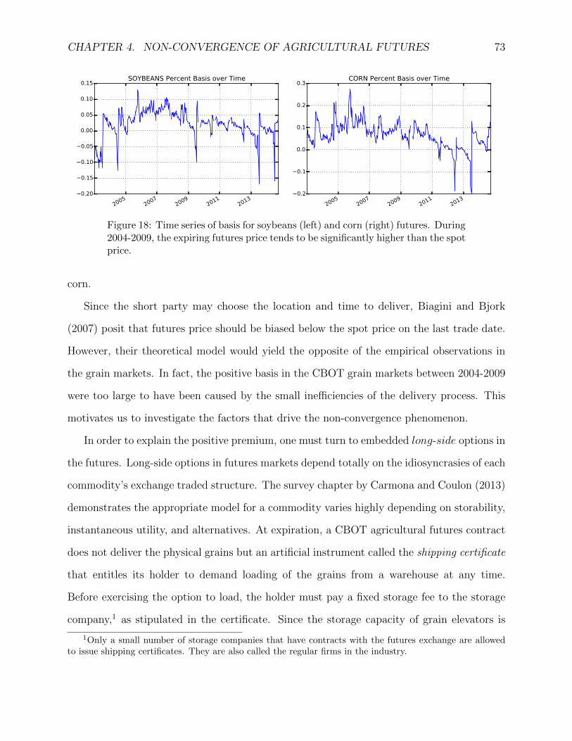
CHAPTER 4. NON-CONVERGENCE OF AGRICULTURAL FUTURES 73
20052007
20092011
20130.20
0.15
0.10
0.05
0.00
0.05
0.10
0.15 SOYBEANS Percent Basis over Time
20052007
20092011
20130.2
0.1
0.0
0.1
0.2
0.3 CORN Percent Basis over Time
Figure 18: Time series of basis for soybeans (left) and corn (right) futures. During2004-2009, the expiring futures price tends to be significantly higher than the spotprice.
corn.
Since the short party may choose the location and time to deliver, Biagini and Bjork
(2007) posit that futures price should be biased below the spot price on the last trade date.
However, their theoretical model would yield the opposite of the empirical observations in
the grain markets. In fact, the positive basis in the CBOT grain markets between 2004-2009
were too large to have been caused by the small inefficiencies of the delivery process. This
motivates us to investigate the factors that drive the non-convergence phenomenon.
In order to explain the positive premium, one must turn to embedded long-side options in
the futures. Long-side options in futures markets depend totally on the idiosyncrasies of each
commodity’s exchange traded structure. The survey chapter by Carmona and Coulon (2013)
demonstrates the appropriate model for a commodity varies highly depending on storability,
instantaneous utility, and alternatives. At expiration, a CBOT agricultural futures contract
does not deliver the physical grains but an artificial instrument called the shipping certificate
that entitles its holder to demand loading of the grains from a warehouse at any time.
Before exercising the option to load, the holder must pay a fixed storage fee to the storage
company,1 as stipulated in the certificate. Since the storage capacity of grain elevators is
1Only a small number of storage companies that have contracts with the futures exchange are allowedto issue shipping certificates. They are also called the regular firms in the industry.
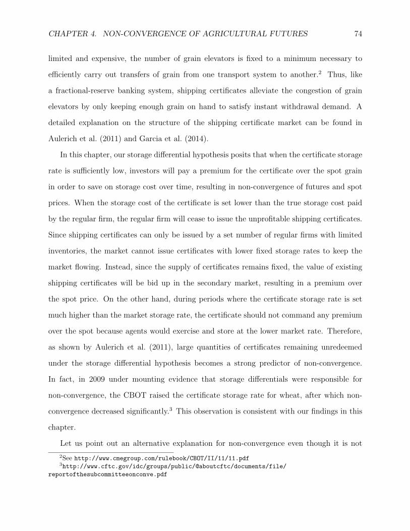
CHAPTER 4. NON-CONVERGENCE OF AGRICULTURAL FUTURES 74
limited and expensive, the number of grain elevators is fixed to a minimum necessary to
efficiently carry out transfers of grain from one transport system to another.2 Thus, like
a fractional-reserve banking system, shipping certificates alleviate the congestion of grain
elevators by only keeping enough grain on hand to satisfy instant withdrawal demand. A
detailed explanation on the structure of the shipping certificate market can be found in
Aulerich et al. (2011) and Garcia et al. (2014).
In this chapter, our storage differential hypothesis posits that when the certificate storage
rate is sufficiently low, investors will pay a premium for the certificate over the spot grain
in order to save on storage cost over time, resulting in non-convergence of futures and spot
prices. When the storage cost of the certificate is set lower than the true storage cost paid
by the regular firm, the regular firm will cease to issue the unprofitable shipping certificates.
Since shipping certificates can only be issued by a set number of regular firms with limited
inventories, the market cannot issue certificates with lower fixed storage rates to keep the
market flowing. Instead, since the supply of certificates remains fixed, the value of existing
shipping certificates will be bid up in the secondary market, resulting in a premium over
the spot price. On the other hand, during periods where the certificate storage rate is set
much higher than the market storage rate, the certificate should not command any premium
over the spot because agents would exercise and store at the lower market rate. Therefore,
as shown by Aulerich et al. (2011), large quantities of certificates remaining unredeemed
under the storage differential hypothesis becomes a strong predictor of non-convergence.
In fact, in 2009 under mounting evidence that storage differentials were responsible for
non-convergence, the CBOT raised the certificate storage rate for wheat, after which non-
convergence decreased significantly.3 This observation is consistent with our findings in this
chapter.
Let us point out an alternative explanation for non-convergence even though it is not
2See http://www.cmegroup.com/rulebook/CBOT/II/11/11.pdf3http://www.cftc.gov/idc/groups/public/@aboutcftc/documents/file/
reportofthesubcommitteeonconve.pdf
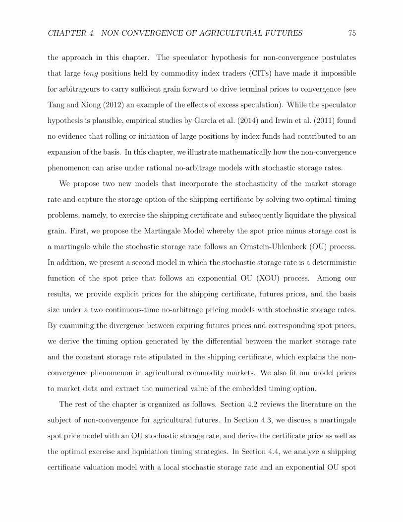
CHAPTER 4. NON-CONVERGENCE OF AGRICULTURAL FUTURES 75
the approach in this chapter. The speculator hypothesis for non-convergence postulates
that large long positions held by commodity index traders (CITs) have made it impossible
for arbitrageurs to carry sufficient grain forward to drive terminal prices to convergence (see
Tang and Xiong (2012) an example of the effects of excess speculation). While the speculator
hypothesis is plausible, empirical studies by Garcia et al. (2014) and Irwin et al. (2011) found
no evidence that rolling or initiation of large positions by index funds had contributed to an
expansion of the basis. In this chapter, we illustrate mathematically how the non-convergence
phenomenon can arise under rational no-arbitrage models with stochastic storage rates.
We propose two new models that incorporate the stochasticity of the market storage
rate and capture the storage option of the shipping certificate by solving two optimal timing
problems, namely, to exercise the shipping certificate and subsequently liquidate the physical
grain. First, we propose the Martingale Model whereby the spot price minus storage cost is
a martingale while the stochastic storage rate follows an Ornstein-Uhlenbeck (OU) process.
In addition, we present a second model in which the stochastic storage rate is a deterministic
function of the spot price that follows an exponential OU (XOU) process. Among our
results, we provide explicit prices for the shipping certificate, futures prices, and the basis
size under a two continuous-time no-arbitrage pricing models with stochastic storage rates.
By examining the divergence between expiring futures prices and corresponding spot prices,
we derive the timing option generated by the differential between the market storage rate
and the constant storage rate stipulated in the shipping certificate, which explains the non-
convergence phenomenon in agricultural commodity markets. We also fit our model prices
to market data and extract the numerical value of the embedded timing option.
The rest of the chapter is organized as follows. Section 4.2 reviews the literature on the
subject of non-convergence for agricultural futures. In Section 4.3, we discuss a martingale
spot price model with an OU stochastic storage rate, and derive the certificate price as well as
the optimal exercise and liquidation timing strategies. In Section 4.4, we analyze a shipping
certificate valuation model with a local stochastic storage rate and an exponential OU spot

CHAPTER 4. NON-CONVERGENCE OF AGRICULTURAL FUTURES 76
price. Section 4.5 concludes. Proofs are provided in the Appendix.
4.2 Related Studies
The long history of the theory of storage dates back to Kaldor (1939) who argued that the
future price should reflect the spot price plus storage cost via a no-arbitrage relationship.
Johnson (1960) proposed an extension of Kaldor’s model which related inventories and hedg-
ing motivations to the intersection of futures and spot markets. However, in order to account
for possibly backwardated futures curves, Brennan (1958) and Working (1949) developed the
notion of a stochastic convenience yield, a fictitious dividend that accrues to the commodity
holder, but not the futures holder. Furthermore, Fama and French (1987) and Gorton et al.
(2012) found plenty of empirical evidence for the theory of storage by examining inventories
data. These authors not only created a theoretical basis for understanding commodity spot
and futures prices, but also empirically demonstrated the validity of the theory of storage
over a century.
Much of the literature on embedded options in futures contracts studies the short-side
options which lower the futures price below the spot price. For example, Hranaiova et al.
(2005) estimate the values of the delivery option, which allows the short to choose the location
of cheapest delivery. In addition, Biagini and Bjork (2007) compute model-free futures prices
for the short-side timing option. In contrast, our models explain how the futures price can be
higher than the spot price at maturity. Our proposed approach contributes to the theory of
storage as it provides a new link between the futures and spot markets through the storage
cost differential and the associated timing option. In a related study, Hinz and Fehr (2010)
consider the impact of storage cost constraints on commodity options, but their model cannot
account for backwardated futures curves or non-convergence.
Aulerich et al. (2011) consider an alternative model in which non-convergence reflects
the value of an exchange option due to the scarcity of shipping certificate. They incorporate
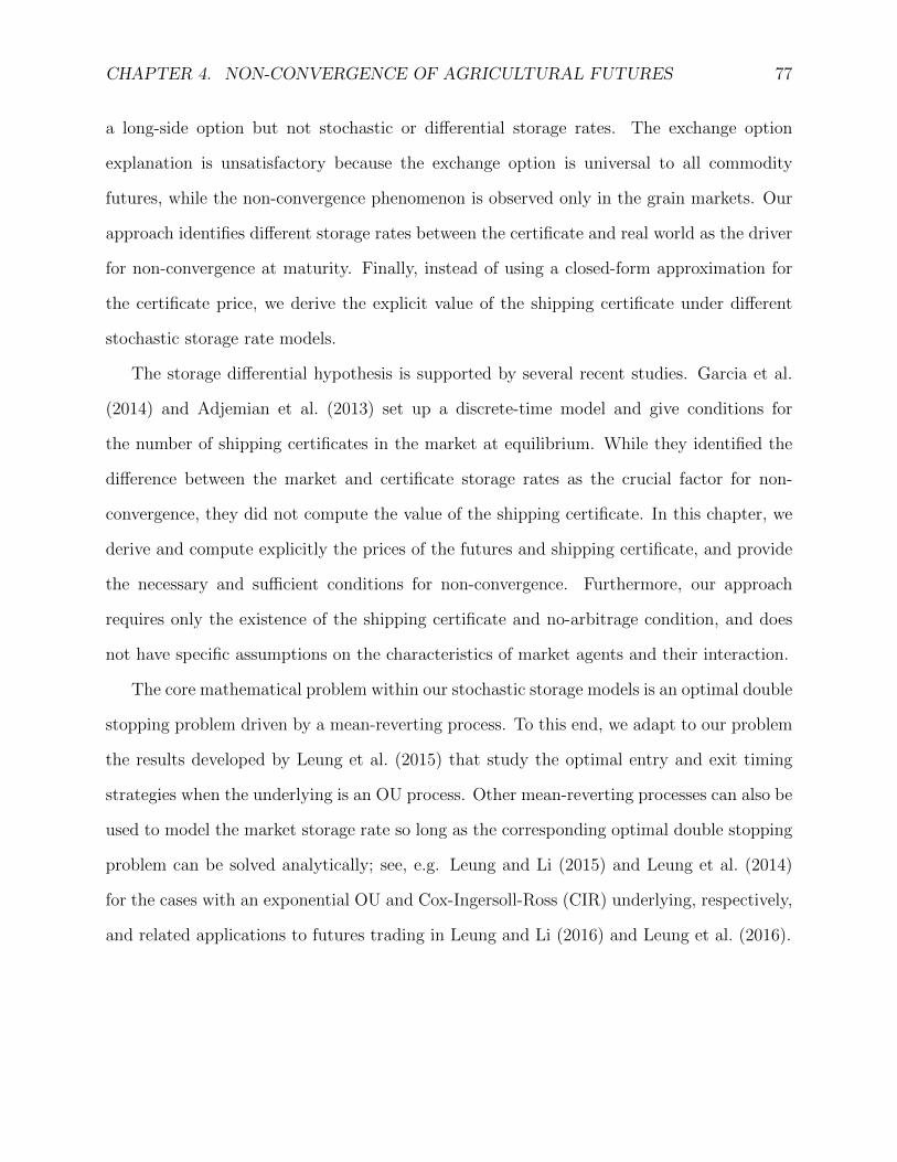
CHAPTER 4. NON-CONVERGENCE OF AGRICULTURAL FUTURES 77
a long-side option but not stochastic or differential storage rates. The exchange option
explanation is unsatisfactory because the exchange option is universal to all commodity
futures, while the non-convergence phenomenon is observed only in the grain markets. Our
approach identifies different storage rates between the certificate and real world as the driver
for non-convergence at maturity. Finally, instead of using a closed-form approximation for
the certificate price, we derive the explicit value of the shipping certificate under different
stochastic storage rate models.
The storage differential hypothesis is supported by several recent studies. Garcia et al.
(2014) and Adjemian et al. (2013) set up a discrete-time model and give conditions for
the number of shipping certificates in the market at equilibrium. While they identified the
difference between the market and certificate storage rates as the crucial factor for non-
convergence, they did not compute the value of the shipping certificate. In this chapter, we
derive and compute explicitly the prices of the futures and shipping certificate, and provide
the necessary and sufficient conditions for non-convergence. Furthermore, our approach
requires only the existence of the shipping certificate and no-arbitrage condition, and does
not have specific assumptions on the characteristics of market agents and their interaction.
The core mathematical problem within our stochastic storage models is an optimal double
stopping problem driven by a mean-reverting process. To this end, we adapt to our problem
the results developed by Leung et al. (2015) that study the optimal entry and exit timing
strategies when the underlying is an OU process. Other mean-reverting processes can also be
used to model the market storage rate so long as the corresponding optimal double stopping
problem can be solved analytically; see, e.g. Leung and Li (2015) and Leung et al. (2014)
for the cases with an exponential OU and Cox-Ingersoll-Ross (CIR) underlying, respectively,
and related applications to futures trading in Leung and Li (2016) and Leung et al. (2016).

CHAPTER 4. NON-CONVERGENCE OF AGRICULTURAL FUTURES 78
4.3 Martingale Model with Stochastic Storage
We now discuss a futures pricing model for a single grain type, with the spot price process
(St)t≥0. The cost of physical storage is stochastic, represented by the rate process (δt)t≥0.
The spot price satisfies
dSt = (rSt + δt)dt+ σStdWt, (4.3.1)
where r is the positive risk-free rate, σ is the volatility parameter of spot grain, and W is
a standard Brownian motion under the risk-neutral measure Q. In this model, we assume
that the commodity is continuously traded, with units of the commodity constantly being
sold to pay the flat storage rate. Hence, the discounted spot price St net storage cost, i.e.
Mt := e−rtSt −∫ t
0δe−rudu, t ≥ 0, is a Q-martingale.
Note that δt is the net storage cost, which is the true storage cost minus the convenience
yield associated with owning the physical grain. Furthermore, the storage rate δt is quoted
in $/bushel, and not as a proportion of the commodity price. In the standard treatment of
storage rates, agents pay a proportion of the commodity price St per bushel i.e. δt = cSt.
However, since empirical storage rates are quoted in $/bushel and not as a percentage of the
crop, our specification of a flat storage rate δt is realistic and amenable for empirical analysis.
One can view the storage rate δt as a negative dividend rate on the commodity which the
commodity holder pays but the futures holder does not. In our model, the storage cost δt
follows an Ornstein-Uhlenbeck (OU) process
dδt = κ(ν − δt)dt+ ζdWt, (4.3.2)
where W is a standard Brownian motion under Q, and is independent of W . The parameter
κ dictates the speed of mean-reversion for δt, ν is the average value of δt, and ζ is the
volatility of the storage rate δt. The parameters are required to satisfy the condition 2κ ≥ ζ.
The filtration F ≡ (Ft)t≥0 is generated by (St)t≥0 and (δt)t≥0. We let T be the set of all
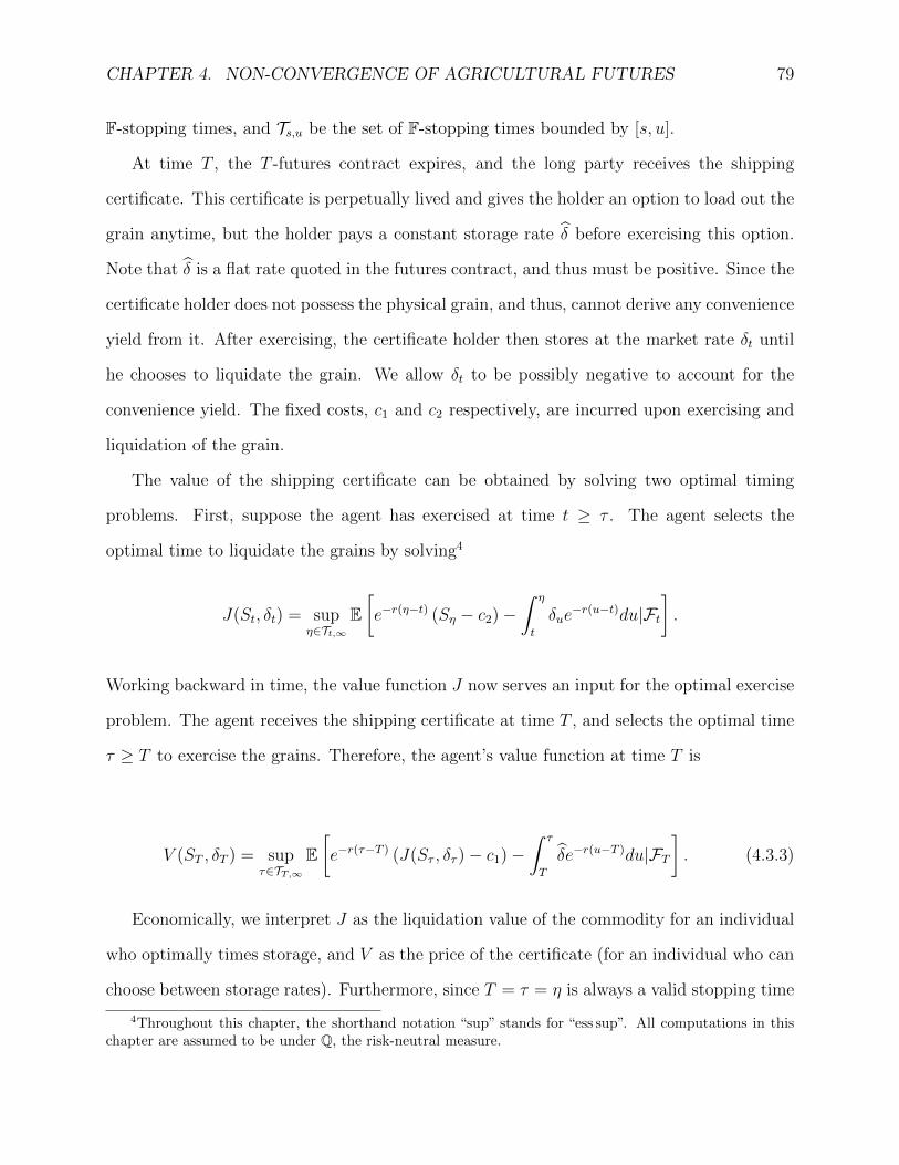
CHAPTER 4. NON-CONVERGENCE OF AGRICULTURAL FUTURES 79
F-stopping times, and Ts,u be the set of F-stopping times bounded by [s, u].
At time T , the T -futures contract expires, and the long party receives the shipping
certificate. This certificate is perpetually lived and gives the holder an option to load out the
grain anytime, but the holder pays a constant storage rate δ before exercising this option.
Note that δ is a flat rate quoted in the futures contract, and thus must be positive. Since the
certificate holder does not possess the physical grain, and thus, cannot derive any convenience
yield from it. After exercising, the certificate holder then stores at the market rate δt until
he chooses to liquidate the grain. We allow δt to be possibly negative to account for the
convenience yield. The fixed costs, c1 and c2 respectively, are incurred upon exercising and
liquidation of the grain.
The value of the shipping certificate can be obtained by solving two optimal timing
problems. First, suppose the agent has exercised at time t ≥ τ . The agent selects the
optimal time to liquidate the grains by solving4
J(St, δt) = supη∈Tt,∞
E[e−r(η−t) (Sη − c2)−
∫ η
t
δue−r(u−t)du|Ft
].
Working backward in time, the value function J now serves an input for the optimal exercise
problem. The agent receives the shipping certificate at time T , and selects the optimal time
τ ≥ T to exercise the grains. Therefore, the agent’s value function at time T is
V (ST , δT ) = supτ∈TT,∞
E[e−r(τ−T ) (J(Sτ , δτ )− c1)−
∫ τ
T
δe−r(u−T )du|FT]. (4.3.3)
Economically, we interpret J as the liquidation value of the commodity for an individual
who optimally times storage, and V as the price of the certificate (for an individual who can
choose between storage rates). Furthermore, since T = τ = η is always a valid stopping time
4Throughout this chapter, the shorthand notation “sup” stands for “ess sup”. All computations in thischapter are assumed to be under Q, the risk-neutral measure.
CHAPTER 4. NON-CONVERGENCE OF AGRICULTURAL FUTURES 80
for (4.3.3), we must have
V (ST , δT ) ≥ ST − c1 − c2.
In the absence of transaction costs, the shipping certificate is valued higher than the grain
itself, and thus the certificate can be considered a long-side option. The value of the long-side
option is quantified with the basis: if T is the maturity of a futures contract, then the basis
w(ST , δT ) is the difference between futures and cash prices at maturity
w(ST , δT ) = V (ST , δT )− ST . (4.3.4)
As the shipping certificate, not the spot grain, is the true delivery instrument, the price
F (t, St, δt;T ) of a futures contract expiring at T satisfies the model-free price
F (t, St, δt;T ) = E[V (ST , δT )|Ft], t ≤ T. (4.3.5)
From this representation, it follows that the expiring futures price equals the certificate price
F (T, ST , δT ;T ) = V (ST , δT ).
Intuitively, the agent decides to liquidate when the spot price is sufficiently high. On
the other hand, the agent may decide to exercise for two reasons: first if the spot price is
sufficiently high, and second if the storage rate δt is sufficiently low relative to the certificate
rate δ. In the first case, the agent exercises and liquidates (i.e. τ ∗ = η∗), and in the second
case, he exercises the shipping certificate but holds the commodity for longer, thus taking
advantage of the lower storage rate δt until the eventual liquidation.
The stochastic storage rate δt is a crucial factor for non-convergence. Indeed, if we instead
consider the simple constant storage rate (δt ≡ δ), then the certificate pricing problem (4.3.3)
CHAPTER 4. NON-CONVERGENCE OF AGRICULTURAL FUTURES 81
simplifies to
V (ST , δT ) = supτ∈TT,∞ η∈Tτ,∞
E[e−r(η−T )Sη −
∫ τ
T
(δ − (c1 + c2)r)e−r(u−T )du
−∫ η
τ
(δ − c2r)e−r(u−T )du|FT
]− c1 − c2.
(4.3.6)
By inspecting the value function in (4.3.6), we see that at every time t, the agent effectively
has a choice between paying the storage rate δ−(c1+c2)r and the storage rate δ−c2r. In other
words, the agent will immediately lock in the lesser of the two rates. If δ − δ ≤ −c1r, then
the agent exercises immediately at expiration (τ ∗ = T ). On the other hand, if δ− δ > −c1r,
then the agent liquidates immediately after uploading (η∗ = τ ∗). We recognize instantly that
under the assumption of constant storage rates at least one stopping time (τ ∗ or η∗) is trivial.
Either the agent exercises immediately, or he liquidates after exercising. In particular, this
fact does not depend at all on the realized path of S. Therefore, a constant storage rate
model is insufficient since the shipping certificate is never used for storing the grain for a non-
trivial period of time. Since certificate holders empirically store and exercise in a multitude
of competitive markets, we must consider a stochastic storage rate δt in all our models.
In order to solve for J and V under the dynamics (4.3.1) and (4.3.2), we need to study
an ODE. Define the differential operator L ≡ La,b,c by
L = a(b− x)d
dx+
1
2c2 d
2
dx2, (4.3.7)
with the generic parameters (a, b, c) with a, c > 0 and b ∈ R. This is the infinitesimal
generator associated with an OU process. In turn, the ODE
Lf(x)− rf(x) = 0
CHAPTER 4. NON-CONVERGENCE OF AGRICULTURAL FUTURES 82
has the two general classical solutions (see e.g. Borodin and Salminen (2002))
H(x; a, b, c) =
∫ ∞0
vra−1e
√2ac2
(x−b)v− v2
2 dv, (4.3.8)
G(x; a, b, c) =
∫ ∞0
vra−1e
√2ac2
(b−x)v− v2
2 dv. (4.3.9)
Direct differentiation yields that H ′(x) > 0, H ′′(x) > 0, G′(x) < 0 and G′′(x) > 0. Hence,
both H(x) and G(x) are strictly positive and convex, and they are, respectively, strictly
increasing and decreasing. Without ambiguity in this section, we denote H(δ) ≡ H(δ;κ, ν, ζ)
andG(δ) ≡ G(δ;κ, ν, ζ) in this section. Alternatively, the functions F andG can be expressed
as
H(x; a, b, c) = exp( a
2c2(x− b)2
)D−r/a
(√2a
c2(b− x)
),
G(x; a, b, c) = exp( a
2c2(x− b)2
)D−r/a
(√2a
c2(x− b)
).
Here, the function D· is also known as parabolic cylinder function or Weber function, whose
properties are elaborated in detail by Erdelyi and Tricom (1953). The functions F and G
will play a crucial role in the solutions for V and J.
Proposition 5. Under the Martingale Model in (4.3.1) and (4.3.2), we have:
1. After the shipping certificate is exercised, it is optimal to never liquidate the grain, and
the value function J(St, δt) = St, for t ≥ T .
2. The value of the shipping certificate is given by
V (St, δt) = St +1
κ+ r
(δt −
H(δt)
H ′(δ∗)− δ +
κ(ν − δ)r
)1δt ≥ δ∗ − c11δt < δ∗,
(4.3.10)
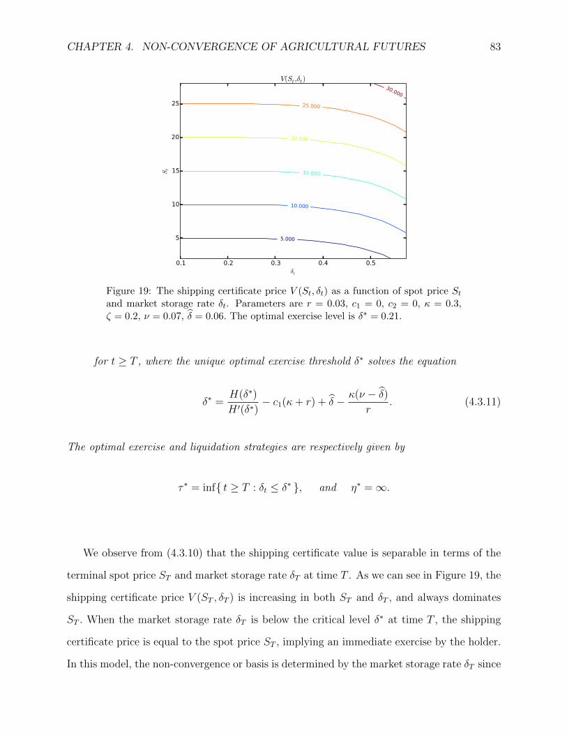
CHAPTER 4. NON-CONVERGENCE OF AGRICULTURAL FUTURES 83
0.1 0.2 0.3 0.4 0.5δt
5
10
15
20
25
St
5.000
10.000
15.000
20.000
25.000
30.000
V(St ,δt)
Figure 19: The shipping certificate price V (St, δt) as a function of spot price Stand market storage rate δt. Parameters are r = 0.03, c1 = 0, c2 = 0, κ = 0.3,ζ = 0.2, ν = 0.07, δ = 0.06. The optimal exercise level is δ∗ = 0.21.
for t ≥ T , where the unique optimal exercise threshold δ∗ solves the equation
δ∗ =H(δ∗)
H ′(δ∗)− c1(κ+ r) + δ − κ(ν − δ)
r. (4.3.11)
The optimal exercise and liquidation strategies are respectively given by
τ ∗ = inf t ≥ T : δt ≤ δ∗ , and η∗ =∞.
We observe from (4.3.10) that the shipping certificate value is separable in terms of the
terminal spot price ST and market storage rate δT at time T . As we can see in Figure 19, the
shipping certificate price V (ST , δT ) is increasing in both ST and δT , and always dominates
ST . When the market storage rate δT is below the critical level δ∗ at time T , the shipping
certificate price is equal to the spot price ST , implying an immediate exercise by the holder.
In this model, the non-convergence or basis is determined by the market storage rate δT since
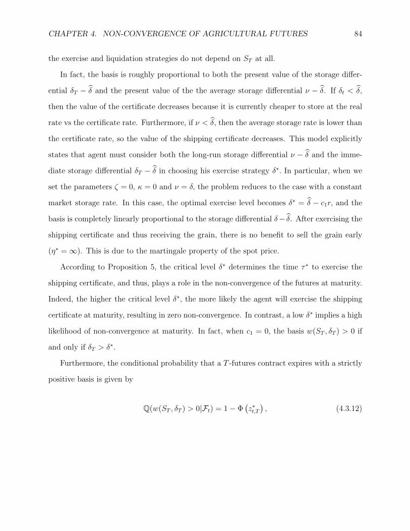
CHAPTER 4. NON-CONVERGENCE OF AGRICULTURAL FUTURES 84
the exercise and liquidation strategies do not depend on ST at all.
In fact, the basis is roughly proportional to both the present value of the storage differ-
ential δT − δ and the present value of the the average storage differential ν − δ. If δt < δ,
then the value of the certificate decreases because it is currently cheaper to store at the real
rate vs the certificate rate. Furthermore, if ν < δ, then the average storage rate is lower than
the certificate rate, so the value of the shipping certificate decreases. This model explicitly
states that agent must consider both the long-run storage differential ν − δ and the imme-
diate storage differential δT − δ in choosing his exercise strategy δ∗. In particular, when we
set the parameters ζ = 0, κ = 0 and ν = δ, the problem reduces to the case with a constant
market storage rate. In this case, the optimal exercise level becomes δ∗ = δ − c1r, and the
basis is completely linearly proportional to the storage differential δ− δ. After exercising the
shipping certificate and thus receiving the grain, there is no benefit to sell the grain early
(η∗ =∞). This is due to the martingale property of the spot price.
According to Proposition 5, the critical level δ∗ determines the time τ ∗ to exercise the
shipping certificate, and thus, plays a role in the non-convergence of the futures at maturity.
Indeed, the higher the critical level δ∗, the more likely the agent will exercise the shipping
certificate at maturity, resulting in zero non-convergence. In contrast, a low δ∗ implies a high
likelihood of non-convergence at maturity. In fact, when c1 = 0, the basis w(ST , δT ) > 0 if
and only if δT > δ∗.
Furthermore, the conditional probability that a T -futures contract expires with a strictly
positive basis is given by
Q(w(ST , δT ) > 0|Ft) = 1− Φ(z∗t,T), (4.3.12)
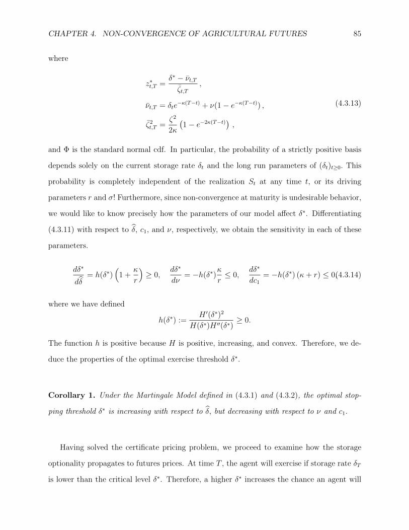
CHAPTER 4. NON-CONVERGENCE OF AGRICULTURAL FUTURES 85
where
z∗t,T =δ∗ − νt,Tζt,T
,
νt,T = δte−κ(T−t) + ν(1− e−κ(T−t)) ,
ζ2t,T =
ζ2
2κ
(1− e−2κ(T−t)) ,
(4.3.13)
and Φ is the standard normal cdf. In particular, the probability of a strictly positive basis
depends solely on the current storage rate δt and the long run parameters of (δt)t≥0. This
probability is completely independent of the realization St at any time t, or its driving
parameters r and σ! Furthermore, since non-convergence at maturity is undesirable behavior,
we would like to know precisely how the parameters of our model affect δ∗. Differentiating
(4.3.11) with respect to δ, c1, and ν, respectively, we obtain the sensitivity in each of these
parameters.
dδ∗
dδ= h(δ∗)
(1 +
κ
r
)≥ 0,
dδ∗
dν= −h(δ∗)
κ
r≤ 0,
dδ∗
dc1
= −h(δ∗) (κ+ r) ≤ 0,(4.3.14)
where we have defined
h(δ∗) :=H ′(δ∗)2
H(δ∗)H ′′(δ∗)≥ 0.
The function h is positive because H is positive, increasing, and convex. Therefore, we de-
duce the properties of the optimal exercise threshold δ∗.
Corollary 1. Under the Martingale Model defined in (4.3.1) and (4.3.2), the optimal stop-
ping threshold δ∗ is increasing with respect to δ, but decreasing with respect to ν and c1.
Having solved the certificate pricing problem, we proceed to examine how the storage
optionality propagates to futures prices. At time T , the agent will exercise if storage rate δT
is lower than the critical level δ∗. Therefore, a higher δ∗ increases the chance an agent will

CHAPTER 4. NON-CONVERGENCE OF AGRICULTURAL FUTURES 86
exercise the shipping certificate immediately upon the futures expiration. A higher certificate
storage rate δ increases δ∗ and hence lowers the probability of non-convergence. On the other
hand, a higher average storage rate ν increases the probability of non-convergence. This
occurs due to the incentive to store in the cheaper market: if the certificate storage rate is
higher (resp. lower) than the market rate, then the agent will exercise sooner (resp. lower).
When calculating the derivatives in (4.3.14), the magnitude of each derivative is roughly
proportional to κ, the rate of mean reversion of the storage rate δt. Indeed, as κ increases,
the long run effect of ν dominates, acting as an amplifier on δ∗. Therefore, under higher κ, if
the storage differential ν− δ is positive, the basis increases more, whereas if ν− δ is negative,
the basis increases less. Intuitively, since the value c1 increases the agent’s cost to exercise,
it is expected, as seen in (4.3.14), that δ∗ is decreasing in c1. Lastly, after exercising, the
agent’s liquidation timing η∗ is trivial, so the liquidation cost c2 does not affect the exercise
level δ∗.
Next, we compute the futures price using the shipping certificate price given in Propo-
sition 5. It follows from the property of the OU process that δT |δt is normally distributed
with parameters νt,T and ζt,T which are given in (4.3.13). Following the definition in (4.3.5),
the futures price is given by
F (t, St, δt;T ) = E [ST |Ft] +1
κ+ rE
[(δT −
H(δT )
H(δ∗)− δ +
κ(ν − δ)r
)1δT ≥ δ∗|Ft
]
− c1Q(δT < δ∗|Ft) .
By computing the conditional truncated expectations of ST and δT , we obtain an explicit
formula for the futures price.

CHAPTER 4. NON-CONVERGENCE OF AGRICULTURAL FUTURES 87
Corollary 2. Under the Martingale Model defined in (4.3.1) and (4.3.2), the grain futures
price is given by
F (t, St, δt;T ) = er(T−t)[St +
ν
r
(1− e−r(T−t)
)+δt − νκ+ r
(1− e−(κ+r)(T−t))]
+1
κ+ r
[νt,T +
φ(z∗t,T)
1− Φ(z∗t,T) ζt,T − ∫ ∞
z∗t,T
H(νt,T + ζt,Tu)
H ′(δ∗)φ(u)du
+
(κ(ν − δ)
r− δ)(
1− Φ(z∗t,T))]− c1Φ
(z∗t,T), t ≤ T, (4.3.15)
where z∗t,T , νt,T and ζt,T are given in (4.3.13), and φ and Φ are the standard normal pdf and
cdf respectively.
We note that like the shipping certificate prices, futures prices can be separated into an
expectation that depends on St and another involving δt. Despite the separation, since δt
appears in the diffusion for St, the two stochastic factors are not independent. The futures
price encapsulates a number of components: (i) the risk-neutral expectation of the future spot
price; (ii) expected future basis w(ST , δT ) (see (4.3.4)); and (iii) expected future exercise cost
c2. Thus, by accounting for the expected future basis resulting from the storage differential
δt− δ, the futures price for all t ≤ T in a market with shipping certificates carries a premium
over the price of a futures contract that delivers just the grain at time T . We therefore
demonstrate that anticipated future storage differentials can impact current futures prices,
including the contracts that are far from expiry.
With an understanding on the theoretical behavior of grain futures prices under the
Martingale Model, we now calibrate to empirical data, and discuss the results and economic
implications. We obtain futures prices from 2004-2011 for CBOT corn, wheat and soybeans
contracts using Bloomberg terminal. We obtain spot prices from 2004-2011 for CBOT corn,
CHAPTER 4. NON-CONVERGENCE OF AGRICULTURAL FUTURES 88
wheat, and soybeans from an average of daily sale prices of several Illinois grain depots.5
We also obtain the empirical certificate storage rate δ, quoted in $/bushel, from the CBOT
website.6,7 For the interest rate in our model, we use the 3-month LIBOR rate observed on
the same date. There are several quoted prices for spot grain, differing only in the quality
of the grain. This quality option allows the short to choose the grade he wishes to deliver,
subject to some prior fixed conversion multiplier of the settlement price. In order to obtain
a single series of spot prices, for every time t we use the then cheapest-to-deliver price as the
spot price for grain.
Recall that the basis w(ST , δT ) is the premium of the certificate price V (T, ST ) over the
spot price ST . at time T . On the day t = 0, we have the empirical futures prices (Fk)Nk=0
with maturities (Tk)Nk=0, and a known spot price F0 = S0; we seek a model-consistent futures
curve Fk(ν, κ, ζ, δ0) for k = 0, 1, . . . , N which best fits the empirical futures prices, given
model parameters (ν, κ, ζ) and δ0, with the model futures prices given in (4.3.15). Under
this setup, the best fit calibrated futures curve F∗k for k = 0, 1, . . . , N minimizes the sum
of squared errors (SSE) between the empirical futures curve and the model futures curve.
Furthermore, the best-fit parameters are defined to be (ν∗, κ∗, ζ∗, δ∗0) the model parameters
which achieve the best fit futures curve. The other exogenous parameters (r, St, δ, c1, c2) are
directly determined via contract specifications. Precisely, the calibrated parameters and the
resulting futures curve are found from
(ν∗, κ∗, ζ∗, δ∗0) = arg minν,κ,ζ,δ0
N∑k=0
(Fk − Fk(ν, κ, ζ, δ0))2
F∗k = ~F(ν∗, κ∗, ζ∗, δ∗0) k = 0, 1, . . . N.
5http://www.farmdoc.illinois.edu/MARKETING/INDEX.ASP6http://www.cmegroup.com/rulebook/CBOT/II/$n$/$m$.pdfwhere$(n,m)\in\protect\T1\
textbraceleft(10,10),(11,11),(14,14)\protect\T1\textbraceright.$7As a result of the certificate rate δ increase in 2009, the size of the empirical basis became smaller
afterward. However, a large strictly positive basis can still manifest in the future if the market storage rateδt is significantly higher than the new certificate rate δ.
CHAPTER 4. NON-CONVERGENCE OF AGRICULTURAL FUTURES 89
In Figure 20, we calibrate the Martingale Model to the corn futures prices on two dates
selected to show two characteristically different futures curves. On the left panel, the futures
curve is downward sloping. With the expiring futures price and spot price being $3.17
and $2.81, respectively, a positive basis is observed. Intuitively, given that the current
market storage rate is higher than the certificate rate (δ∗0 > δ), the agent thus prefers the
certificate storage rate over the market rate and will wait to exercise the certificate, resulting
in a positive basis. The current storage rate δ∗0 is also higher than the estimated long-run
storage rate ν∗. Therefore, the model suggests that in the long run, a convenience yield will
dominate, leading to a downward sloping futures curve. In contrast, the right panel also
reflects a positive basis, but the futures curve is upward sloping.
Figure 21 displays the calibrated futures curves under the Martingale Model for wheat on
two dates when the futures market is in backwardation and contango, respectively. Again,
non-convergence is observed on each of these two dates as the expiring futures price dominates
the spot price. On the left panel, the futures curve is upward sloping while the right panel
shows that the futures curve is downward sloping. In this case, the current market storage
rate satisfies δ∗0 > δ, so it is optimal for the agent to continue to store at the lower certificate
storage rate. Hence, the value of the associated timing option to exercise the shipping
certificate yields a positive basis.
In addition, we consider the differences between the model futures curve and the futures
curve generated without considering the timing options. To be precise, let the ‘no certificate’
futures price ψ(t, St, δt;T ) be
ψ(t, St, δt;T ) = E[ST |Ft],
= er(T−t)[St +
ν
r
(1− e−r(T−t)
)+δt − νκ+ r
(1− e−(κ+r)(T−t))] . (4.3.16)
This follows from direct calculations and resembles the first line of (4.3.15). In Figure 20, we
plot the values of ψ(0, S0, δ∗0;Ti) for i = 0 . . . N, using the same fitted parameters from our
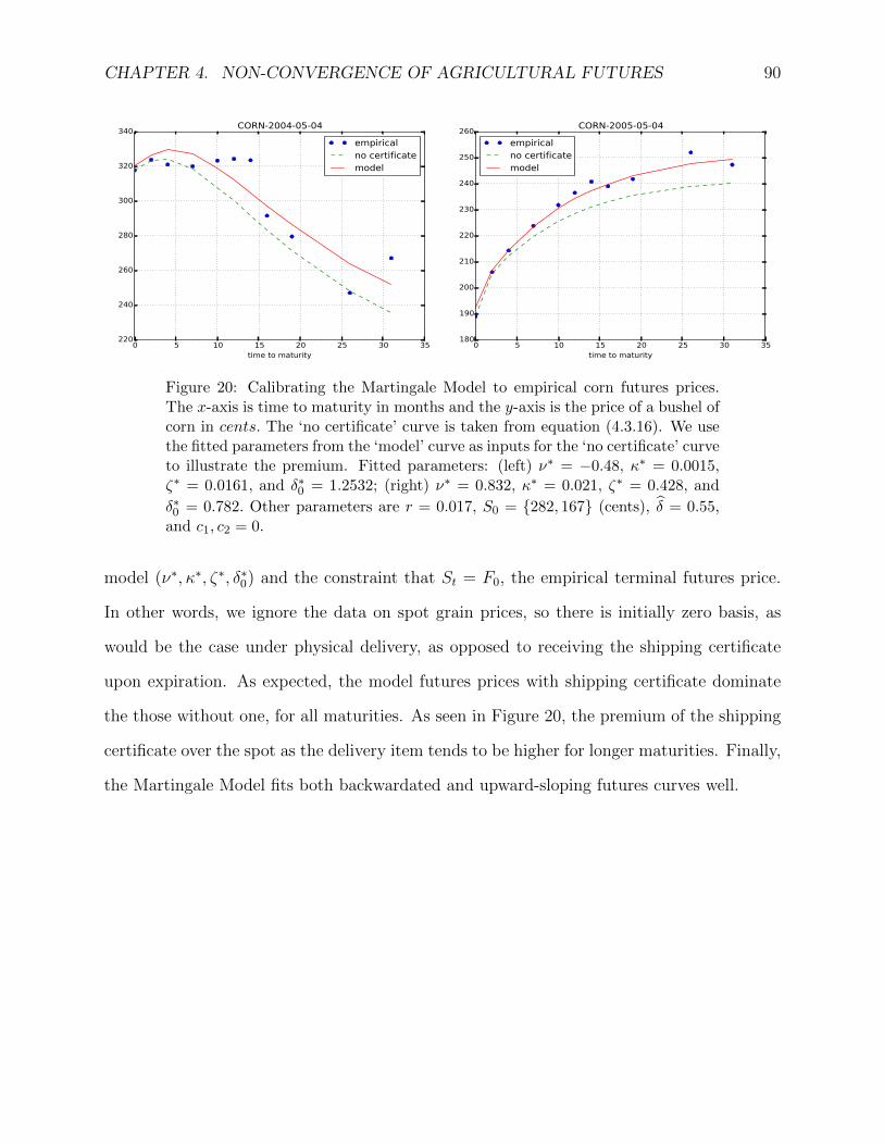
CHAPTER 4. NON-CONVERGENCE OF AGRICULTURAL FUTURES 90
0 5 10 15 20 25 30 35time to maturity
220
240
260
280
300
320
340 CORN-2004-05-04
empiricalno certificatemodel
0 5 10 15 20 25 30 35time to maturity
180
190
200
210
220
230
240
250
260 CORN-2005-05-04
empiricalno certificatemodel
Figure 20: Calibrating the Martingale Model to empirical corn futures prices.The x-axis is time to maturity in months and the y-axis is the price of a bushel ofcorn in cents. The ‘no certificate’ curve is taken from equation (4.3.16). We usethe fitted parameters from the ‘model’ curve as inputs for the ‘no certificate’ curveto illustrate the premium. Fitted parameters: (left) ν∗ = −0.48, κ∗ = 0.0015,ζ∗ = 0.0161, and δ∗0 = 1.2532; (right) ν∗ = 0.832, κ∗ = 0.021, ζ∗ = 0.428, and
δ∗0 = 0.782. Other parameters are r = 0.017, S0 = 282, 167 (cents), δ = 0.55,and c1, c2 = 0.
model (ν∗, κ∗, ζ∗, δ∗0) and the constraint that St = F0, the empirical terminal futures price.
In other words, we ignore the data on spot grain prices, so there is initially zero basis, as
would be the case under physical delivery, as opposed to receiving the shipping certificate
upon expiration. As expected, the model futures prices with shipping certificate dominate
the those without one, for all maturities. As seen in Figure 20, the premium of the shipping
certificate over the spot as the delivery item tends to be higher for longer maturities. Finally,
the Martingale Model fits both backwardated and upward-sloping futures curves well.

CHAPTER 4. NON-CONVERGENCE OF AGRICULTURAL FUTURES 91
0 5 10 15 20 25 30time to maturity
300
310
320
330
340
350
360 WHEAT-2005-05-04
empiricalno certificatemodel
0 5 10 15 20 25 30 35time to maturity
650
700
750
800
850
900 WHEAT-2007-11-23
empiricalno certificatemodel
Figure 21: Calibrating the Martingale Model to empirical wheat futures prices.The x-axis is time to maturity in months and the y-axis is the price of a bushel ofwheat in cents. The ‘no certificate’ curve is taken from equation (4.3.16). Fittedparameters: (left) ν∗ = 0.91, κ∗ = 0.035, ζ∗ = 0.14, and δ∗0 = 0.871; (right)ν∗ = −0.22, κ∗ = 0.0032, ζ∗ = 0.61, and δ∗0 = 1.44. We use the fitted parametersfrom the ‘model’ curve as inputs for the ‘no certificate’ curve to illustrate thepremium. Other parameters are r = 0.017, S0 = 273, 772 (cents), δ = 0.55,and c1, c2 = 0.
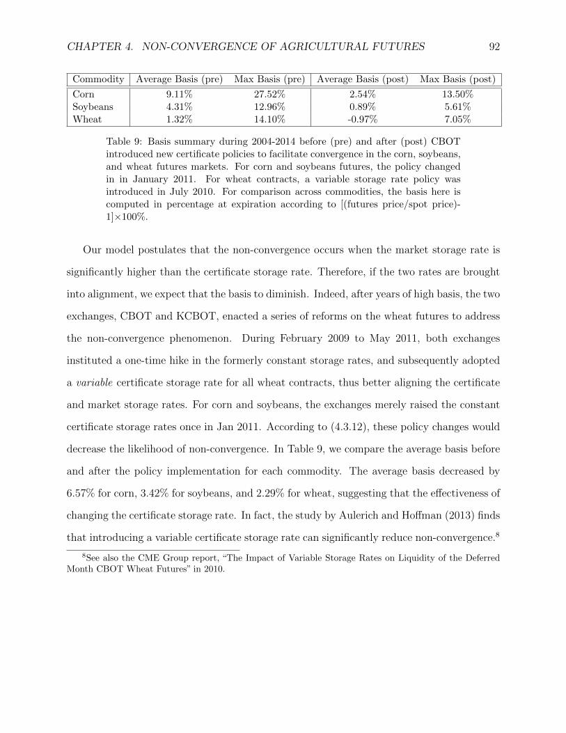
CHAPTER 4. NON-CONVERGENCE OF AGRICULTURAL FUTURES 92
Commodity Average Basis (pre) Max Basis (pre) Average Basis (post) Max Basis (post)
Corn 9.11% 27.52% 2.54% 13.50%Soybeans 4.31% 12.96% 0.89% 5.61%Wheat 1.32% 14.10% -0.97% 7.05%
Table 9: Basis summary during 2004-2014 before (pre) and after (post) CBOTintroduced new certificate policies to facilitate convergence in the corn, soybeans,and wheat futures markets. For corn and soybeans futures, the policy changedin in January 2011. For wheat contracts, a variable storage rate policy wasintroduced in July 2010. For comparison across commodities, the basis here iscomputed in percentage at expiration according to [(futures price/spot price)-1]×100%.
Our model postulates that the non-convergence occurs when the market storage rate is
significantly higher than the certificate storage rate. Therefore, if the two rates are brought
into alignment, we expect that the basis to diminish. Indeed, after years of high basis, the two
exchanges, CBOT and KCBOT, enacted a series of reforms on the wheat futures to address
the non-convergence phenomenon. During February 2009 to May 2011, both exchanges
instituted a one-time hike in the formerly constant storage rates, and subsequently adopted
a variable certificate storage rate for all wheat contracts, thus better aligning the certificate
and market storage rates. For corn and soybeans, the exchanges merely raised the constant
certificate storage rates once in Jan 2011. According to (4.3.12), these policy changes would
decrease the likelihood of non-convergence. In Table 9, we compare the average basis before
and after the policy implementation for each commodity. The average basis decreased by
6.57% for corn, 3.42% for soybeans, and 2.29% for wheat, suggesting that the effectiveness of
changing the certificate storage rate. In fact, the study by Aulerich and Hoffman (2013) finds
that introducing a variable certificate storage rate can significantly reduce non-convergence.8
8See also the CME Group report, “The Impact of Variable Storage Rates on Liquidity of the DeferredMonth CBOT Wheat Futures” in 2010.
CHAPTER 4. NON-CONVERGENCE OF AGRICULTURAL FUTURES 93
4.4 Local Stochastic Storage Model
We now consider an alternative to the Martingale Model. Since the commodity cannot
necessarily be continuously traded, the market is incomplete, and one can specify a non-
martingale evolution for the commodity price under the no-arbitrage risk-neutral measure.
Commodities have the unique property that production can be increased or decreased in
response to high or low prices, respectively. In addition, commodities can be consumed
through production of end-goods (for example, turning corn into ethanol). In times of
scarcity, production will increase to lower prices; in times of surplus, production will decrease
while consumption continues to increase prices. Thus, the production and consumption
process unique to commodities imply a mean-reverting price structure as suggested by Deaton
and Laroque (1996).
Hence, we propose an exponential OU (XOU) model for the spot price. Under the risk-
neutral measure Q, the log-spot price of the grain, denoted by Ut = logSt, follows the OU
process
dUt = α(µ− Ut)dt+ σdWt, (4.4.1)
where W is standard Brownian motion under Q, µ is the long-run mean, α is the rate of
mean reversion, and σ is the volatility of the log-spot price. We impose the further regularity
condition that σ <√
2α.
The market rate of storage δt is locally determined by the spot price through
δt = βUt + γ. (4.4.2)
We typically set the coefficient β ≥ 0 so that the storage cost increases linearly with the
log-price of the commodity, with a possibly flat storage rate γ > 0. In summary, we have
described a local stochastic storage approach, whereby the market storage rate in (4.4.2)
is a function of the stochastic spot price that follows the exponential OU model in (4.4.1).
CHAPTER 4. NON-CONVERGENCE OF AGRICULTURAL FUTURES 94
Henceforth, we shall refer it as the XOU Model.
Denote by G ≡ (Gt)t≥0 the filtration generated by the log-spot price (Ut)t≥0. Also, let S
be the set of all G-stopping times, and Ss,u the set of G-stopping times bounded by [s, u].
Note that δt is a function of Ut, the optimal liquidation problem is given by
J(Ut) = supη∈St,∞
E[e−r(η−t) (exp(Uη)− c2)−
∫ η
t
δue−r(u−t)du|Gt
],
which applies after the shipping certificate is exercised at time τ . The optimal timing problem
to exercise the shipping certificate is given by
V (UT ) = supτ∈ST,∞
E[e−r(τ−T ) (J(Uτ )− c1)−
∫ τ
T
δe−r(u−T )du|GT].
Since the shipping certificate serves as the delivery item instead of the actual grain, the
futures price F (t, Ut;T ) at t for the contract expiring at T is given by
F (t, Ut;T ) = E[V (UT )|Gt].
We now denote the operator from (4.3.7) by L ≡ Lα,µ,σ, which is the infinitesimal gener-
ator for the OU process U . To solve for the certificate price and the agent’s optimal policy,
we solve the ODE
Lf(u)− rf(u) = 0,
which has the general solutions, H(u;α, µ, σ) and G(u;α, µ, σ), where L, H, and G are
defined in (4.3.7), (4.3.8) and (4.3.9). In this section, without ambiguity, we denote H(u) ≡
H(u;α, µ, σ) and G(u) ≡ G(u;α, µ, σ), both of which will play a role in the solution for J
and V.
Proposition 6. Under the XOU Model defined in (4.4.1) and (4.4.2):
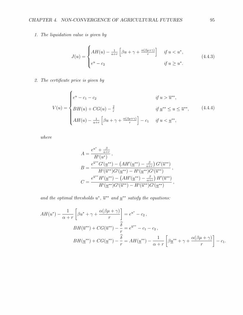
CHAPTER 4. NON-CONVERGENCE OF AGRICULTURAL FUTURES 95
1. The liquidation value is given by
J(u) =
AH(u)− 1
α+r
[βu+ γ + α(βµ+γ)
r
]if u < u∗,
eu − c2 if u ≥ u∗.
(4.4.3)
2. The certificate price is given by
V (u) =
eu − c1 − c2 if u > u∗∗,
BH(u) + CG(u)− δr
if u∗∗ ≤ u ≤ u∗∗,
AH(u)− 1α+r
[βu+ γ + α(βµ+γ)
r
]− c1 if u < u∗∗,
(4.4.4)
where
A =eu∗
+ βα+r
H ′(u∗),
B =eu∗∗G′(u∗∗)−
(AH ′(u∗∗)− β
α+r
)G′(u∗∗)
H ′(u∗∗)G′(u∗∗)−H ′(u∗∗)G′(u∗∗) ,
C =eu∗∗H ′(u∗∗)−
(AH ′(u∗∗)− β
α+r
)H ′(u∗∗)
H ′(u∗∗)G′(u∗∗)−H ′(u∗∗)G′(u∗∗) ,
and the optimal thresholds u∗, u∗∗ and u∗∗ satisfy the equations:
AH(u∗)− 1
α + r
[βu∗ + γ +
α(βµ+ γ)
r
]= eu
∗ − c2 ,
BH(u∗∗) + CG(u∗∗)− δ
r= eu
∗∗ − c1 − c2 ,
BH(u∗∗) + CG(u∗∗)− δ
r= AH(u∗∗)− 1
α + r
[βu∗∗ + γ +
α(βµ+ γ)
r
]− c1.
CHAPTER 4. NON-CONVERGENCE OF AGRICULTURAL FUTURES 96
The optimal exercise and liquidation times, respectively, are given by
τ ∗ = inf t ≥ T : Ut ≤ u∗∗ or Ut ≥ u∗∗ ,
η∗ = inf t ≥ τ ∗ : Ut ≥ u∗ .
The liquidation value J(u) is entirely determined by the critical level u∗ at which the
agent will sell the physical grain. When the log-spot price Ut surpasses u∗, both the storage
cost δt and spot price St will be high. Since the asset price is mean-reverting, intuitively
there is a potential advantage to early liquidation before the asset reverts back to a lower
value. In the holding region u < u∗ corresponding to low spot prices, the agent pays the
present value of the storage rate βu + γ, and the present value of the average storage rate
βµ+ γ. The conflict between increasing spot prices and higher storage rates, both of which
are driven by Ut, determines when the agent liquidates. Thus, both instantaneous storage
rates and the long-run storage rates affect the certificate price.
On the other hand, the certificate value V (u) is determined by two stopping levels: the
optimal exercise threshold u∗∗ and the optimal liquidation threshold u∗∗. When the spot price
surpasses u∗∗, the agent exercises and liquidates to take advantage of temporarily higher spot
prices, while avoiding higher storage rates. On the other hand, when the spot price decreases
below u∗∗, the agent exercises but does not liquidate, because he wants to take advantage
of a temporarily lower storage rate, storing in the real market at rate δt instead of at the
certificate rate δ. Recall that due to our specification of the optimal stopping times η∗ and
τ ∗, the stopping levels satisfy u∗∗ ≥ u∗ ≥ u∗∗.
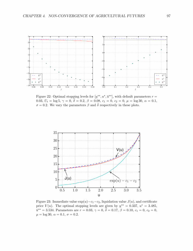
CHAPTER 4. NON-CONVERGENCE OF AGRICULTURAL FUTURES 97
0.06 0.08 0.10 0.12 0.14 0.16 0.18 0.20
β
−4
−3
−2
−1
0
1
2
3
4
u∗∗
u∗
u∗∗
0.0 0.1 0.2 0.3 0.4 0.5
δ
−8
−6
−4
−2
0
2
4
u∗∗
u∗
u∗∗
Figure 22: Optimal stopping levels for [u∗∗, u∗, u∗∗], with default parameters r =0.03, Ut = log 5, γ = 0, δ = 0.2, β = 0.08, c1 = 0, c2 = 0, µ = log 30, α = 0.1,σ = 0.2. We vary the parameters β and δ respectively in these plots.
0.5 1.0 1.5 2.0 2.5 3.0 3.5u
0
5
10
15
20
25
30
35
V(u)
J(u)exp(u)− c1 − c2
Figure 23: Immediate value exp(u)−c1−c2, liquidation value J(u), and certificateprice V (u). The optimal stopping levels are given by u∗∗ = 0.337, u∗ = 3.485,u∗∗ = 3.534. Parameters are r = 0.03, γ = 0, δ = 0.17, β = 0.10, c1 = 0, c2 = 0,µ = log 30, α = 0.1, σ = 0.2.

CHAPTER 4. NON-CONVERGENCE OF AGRICULTURAL FUTURES 98
Figure 22 further illustrates the dependence of the three stopping levels [u∗∗, u∗, u∗∗] on the
parameters β and δ. As β increases, the gap between u∗∗ and u∗∗ increases, so does the basis.
However, as β → 0, the market storage rate goes to 0 in this example, inducing the agent to
exercise as soon as the futures expires and store in the real market. Consequently, the region
u∗∗, u∗∗ for holding the certificate vanishes, which also means that all three thresholds,
u∗∗, u∗, and u∗∗ converge to the same value representing the optimal level to liquidate the
grain. A similar pattern is observed when the certificate storage rate δ increases since the
agent will again be incentivized to exercise the shipping certificate immediately to store in
the real market.
Figure 23 also reflects the relationship among the certificate price, liquidation value, and
payoff from immediate exercise and liquidation. Note that
V (u) ≥ J(u) ≥ exp(u)− c1 − c2,
i.e. the shipping certificate price dominates the liquidation value, which convexly dominates
the immediate exercise value. The liquidation value is significantly higher than the immediate
exercise value, especially as u → −∞. The value of J(u) does not decrease as much as
the immediate exercise value. Because the asset is mean reverting and the optionality is
perpetual, the asset value is almost guaranteed to be eventually profitable. In this model, the
ability to choose between two rates of storage adds merely a modest basis to the liquidation
value. With the parameters in Figure 22, the maximum percent difference between V (u)
and J(u) is 12.57%.
Recall that the basis w(Ut) is defined as the difference between certificate and spot prices
at maturity. As we established from a model-free argument, the basis w(Ut) ≥ 0. Therefore,
a positive basis occurs when the agent chooses a strategy which is different than exercising
and liquidating (η∗ > τ > T ). In this scenario, the agent either waits to exercise because
storage rates are too high to exercise and spot prices are too low to liquidate, or he has
CHAPTER 4. NON-CONVERGENCE OF AGRICULTURAL FUTURES 99
exercised to take advantage of lower storage prices but the spot price is too low to liquidate.
In our model the probability of non-convergence depends completely on u∗∗. In particular, if
c1 = 0 and c2 = 0, then the basis w(UT ) > 0 iff UT < u∗∗. Thus, the probability that there
is a strictly positive basis at time t for a contract maturing at T ≥ t is
Q (w(UT ) > 0 | Gt) = Φ
(u∗∗ − µt,T
σt,T
),
where
µt,T = Ute−α(T−t) + µ(1− e−α(T−t)),
σ2t,T =
σ2
2α(1− e−2α(T−t)).
(4.4.5)
Finally, in order to calibrate our model for empirical analysis, we derive futures prices by
taking an expectation of the certificate prices.
Under the OU model, the conditional log spot price UT |Ut is normally distributed with
parameters µt,T and σt,T given in (4.4.5). The result then follows from computing the asso-
ciated conditional truncated expectations:
F (t, Ut;T ) = E[(eUT − c1 − c2
)1UT > u∗∗|Ut
]+ E
[(BH(UT ) + CG(UT )− δ
r
)1u∗∗ ≤ UT ≤ u∗∗|Ut
]
+ E[(AH(u)− 1
α + r
[βUT + γ +
α(βµ+ γ)
r
]− c1
)1UT < u∗∗|Ut
]
Corollary 3. The futures price F (t, Ut;T ) under the XOU Model defined in (4.4.1) and
(4.4.2) is given by
CHAPTER 4. NON-CONVERGENCE OF AGRICULTURAL FUTURES 100
F (t, Ut;T ) = exp
(µt,T +
σ2t,T
2
)Φ(σt,T − z∗∗t,T
)1− Φ
(z∗∗t,T) − (c1 + c2)
(1− Φ
(z∗∗t,T))
+
∫ z∗∗t,T
z∗∗t,T
(BH(µt,T + σt,Tv) + CG(µt,T + σt,Tv))φ(v)dv
− δ
r
(Φ(z∗∗t,T)− Φ
(z∗∗t,T))
+
∫ z∗∗t,T
−∞AH(µt,T + σt,Tv)dv
− β
α + r
(µt,T −
φ(z∗∗t,T)
Φ(z∗∗t,T) σt,T)− ( γ
α + r+α(βµ+ γ)
r(α + r)+ c1
)Φ(z∗∗t,T),
where
z∗∗t,T =u∗∗ − µt,T
σt,T, z∗∗t,T =
u∗∗ − µt,Tσt,T
,
and µt,T , and σt,T are defined in (4.4.5).
We calibrate our model futures curve to empirical corn, wheat and soybeans data and
consider the accuracy and economic implications. Refer to Table 9 for details of each con-
tract’s specification. Consider the futures curve at time t = 0. Recall that the best-fit futures
curve can be defined in the following manner. Let the futures prices at time Tk be Fk, for
maturity times (Tk)Nk=0, with F0 = exp(U0) = S0, so the futures price at T0 = 0 is just the
market quoted settlement price. Denote the model futures curve generated at time Tk by
the parameters (β, γ, µ, α, σ) be denoted Fk(β, γ, µ, α, σ).
The best fit futures curve F∗k for k = 0, 1, . . . , N minimizes the weighted sum of squared
errors (SSE) between the empirical futures curve and the model futures curve at time t.
Furthermore, the best-fit parameter is defined to be (β∗, γ∗, µ∗, α∗, σ∗) the model parameters
which achieve the best fit futures curve. The other exogenous parameters (r, Ut, δ, c1, c2) are

CHAPTER 4. NON-CONVERGENCE OF AGRICULTURAL FUTURES 101
directly determined via contract specifications (see Table 9).
(β∗, γ∗, µ∗, α∗, σ∗) = arg minβ,γ,µ,α,σ
N∑k=0
(Fk − Fk(β, γ, µ, α, σ))2
F∗k = Fk(β∗, γ∗, µ∗, α∗, σ∗) k = 0, 1, . . . , N.
The corn futures curves calibrated from the XOU Model are illustrated in Figure 24. We
have selected the two dates to illustrate two characteristically different futures curves. On
the left panel, the futures curve that is upward sloping. With the expiring futures price and
spot price being 317 and 281 (cents), respectively, a positive basis is observed. The current
storage rate δ∗0 = 106.00, and the long run storage rate β∗µ∗ + γ∗ = 89.55 are both higher
than the certificate rate δ. This storage rate spread leads to the positive basis, while the long
run storage rate anticipates a future basis. Furthermore, the current spot price U0 > µ∗,
which indicates that the spot price will likely fall in the future, and results in a downward-
sloping futures curve. On the right panel, the futures curve is upward sloping and the basis
is more modest. The spot price current satisfies U0 < µ∗, so the spot price is expected to
rise in the future, generating a more contango futures curve.
In Figure 25, we see the results of our empirical calibration under the XOU model for
wheat on two dates. The left panel shows a basis of around 12%, and the futures curve
is upward sloping. The current storage rate δ∗0 = 67.21, and the long run storage rate
β∗µ∗ + γ∗ = 69.84 are both higher than the certificate rate δ. Therefore, the current storage
rate leads to a positive basis, while the long run storage rate anticipates a future basis.
Furthermore, the current spot price U0 < µ∗, which indicates that the spot price will likely
rise in the future, and results in an upward-sloping futures curve. In Figure 25 (right),
the basis is more modest at 5%, while the futures curve is downward sloping. The current
storage rate δ∗0 = 60.71, is higher than the certificate storage rate, but the long run storage
rate β∗µ∗ + γ∗ = 53.87 is lower than the certificate rate δ. Therefore, the current storage
rate generates a smaller positive basis, while the long run storage rate anticipates little to no

CHAPTER 4. NON-CONVERGENCE OF AGRICULTURAL FUTURES 102
basis on the futures curve. Furthermore, the current spot price is higher than the estimated
long-run mean (U0 > µ∗), and the backwardated futures curve reflects the anticipation that
the spot price will decrease in the future. This is consistent with the model’s mean-reverting
dynamics for the spot price.
In addition, we consider the differences between the model futures curve and the futures
curve generated without considering the timing options. To be precise, let the ‘no certificate’
futures curve ψ(t, Ut, δt;T ) be
ψ(t, Ut;T ) = E[ST |Gt]
= exp
(e−α(T−t)Ut + µ(1− e−α(T−t)) +
σ2
4µ(1− e−2α(T−t))
), (4.4.6)
which can be found in (Leung et al., 2016, Sect. 2.2). In Figure 25, we plot the futures curve,
described by ψ(0, U0;Ti) for i = 0 . . . N, using the same fitted parameters from our model
(µ∗, α∗, σ∗) and the initial assumption that exp(U0) = F0, the empirical terminal futures
price. In other words, for the no-certificate case, we take the expiring futures price to be the
spot price, and ignore the entire spot grain market prices. The last assumption means there
is initially zero basis, as would be the case when physical grain is the delivery item.
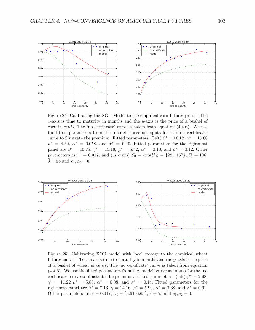
CHAPTER 4. NON-CONVERGENCE OF AGRICULTURAL FUTURES 103
0 5 10 15 20 25 30 35time to maturity
200
220
240
260
280
300
320
340 CORN-2004-05-04
empiricalno certificatemodel
0 5 10 15 20 25 30 35time to maturity
180
190
200
210
220
230
240
250
260 CORN-2005-05-04
empiricalno certificatemodel
Figure 24: Calibrating the XOU Model to the empirical corn futures prices. Thex-axis is time to maturity in months and the y-axis is the price of a bushel ofcorn in cents. The ‘no certificate’ curve is taken from equation (4.4.6). We usethe fitted parameters from the ‘model’ curve as inputs for the ‘no certificate’curve to illustrate the premium. Fitted parameters: (left) β∗ = 16.12, γ∗ = 15.08µ∗ = 4.62, α∗ = 0.058, and σ∗ = 0.40. Fitted parameters for the rightmostpanel are β∗ = 10.75, γ∗ = 15.10, µ∗ = 5.52, α∗ = 0.10, and σ∗ = 0.12. Otherparameters are r = 0.017, and (in cents) S0 = exp(U0) = 281, 167, δ∗0 = 106,
δ = 55 and c1, c2 = 0.
0 5 10 15 20 25 30time to maturity
300
310
320
330
340
350
360 WHEAT-2005-05-04
empiricalno certificatemodel
0 5 10 15 20 25 30 35time to maturity
650
700
750
800
850
900 WHEAT-2007-11-23
empiricalno certificatemodel
Figure 25: Calibrating XOU model with local storage to the empirical wheatfutures curve. The x-axis is time to maturity in months and the y-axis is the priceof a bushel of wheat in cents. The ‘no certificate’ curve is taken from equation(4.4.6). We use the fitted parameters from the ‘model’ curve as inputs for the ‘nocertificate’ curve to illustrate the premium. Fitted parameters: (left) β∗ = 9.98,γ∗ = 11.22 µ∗ = 5.83, α∗ = 0.08, and σ∗ = 0.14. Fitted parameters for therightmost panel are β∗ = 7.13, γ = 14.16, µ∗ = 5.90, α∗ = 0.38, and σ∗ = 0.91.Other parameters are r = 0.017, Ut = 5.61, 6.65, δ = 55 and c1, c2 = 0.

CHAPTER 4. NON-CONVERGENCE OF AGRICULTURAL FUTURES 104
0 2 4 6 8 10 12 14 16 18time to maturity
600
700
800
900
1000
1100 SOYBEANS-2004-05-04
empiricalno certificatemodel
0 2 4 6 8 10 12 14 16 18time to maturity
600
700
800
900
1000
1100 SOYBEANS-2004-05-04
empiricalno certificatemodel
Figure 26: Calibrating the Martingale Model (left) and the XOU Model (right)to the empirical soybeans futures curve. The x-axis is time to maturity in monthsand the y-axis is the price of a bushel of wheat in cents. The ‘no certificate’ curveis taken from equations (4.3.16) and (4.4.6) respectively. The fitted parametersfrom the ‘model’ curve are used as inputs for the ‘no certificate’ curve to illustratethe premium. Fitted parameters: (left) ν∗ = −0.44, κ∗ = 0.023, ζ∗ = 0.92, andδ∗0 = 1.42; (right) β∗ = 11.88, γ∗ = 9.97, µ∗ = 5.91, α∗ = 0.035, and σ∗ = 0.95.
Other parameters are r = 0.017, St = 1004.25, δ = 55 and c1 = c2 = 0.
As shown earlier, the model prices of futures of all maturities with a shipping certificate
dominate the respective contracts without one due to the timing options embedded in the
shipping certificate. Furthermore, the difference increases as the futures maturity lengthens,
indicating that the storage option exerts a more significant price impact over a longer period
of time. In summary, we have shown that the timing options in a shipping certificate are
a crucial component to explain the positive basis. As we have seen, the exponential OU
model is able to capture forward anticipative behaviors of the basis and account for both
backwardated and upwards-sloping futures curves.
We close this section by comparing the empirical calibrations of the Martingale Model
and the XOU Model in Figure 26. While both models are equally capable of estimating
the immediate basis and fitting the empirical futures prices, the value of the timing option
embedded in the shipping certificate is significantly higher under the XOU Model than the
Martingale Model. This can be seen from the spread between the ‘model’ curve (shipping
certificate delivery) and the ‘no certificate’ curve (physical spot delivery) plotted on both
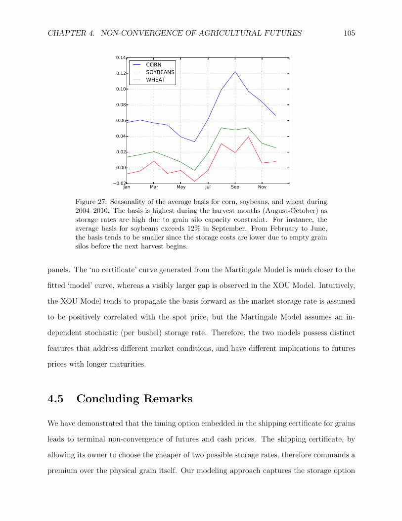
CHAPTER 4. NON-CONVERGENCE OF AGRICULTURAL FUTURES 105
Figure 27: Seasonality of the average basis for corn, soybeans, and wheat during2004–2010. The basis is highest during the harvest months (August-October) asstorage rates are high due to grain silo capacity constraint. For instance, theaverage basis for soybeans exceeds 12% in September. From February to June,the basis tends to be smaller since the storage costs are lower due to empty grainsilos before the next harvest begins.
panels. The ‘no certificate’ curve generated from the Martingale Model is much closer to the
fitted ‘model’ curve, whereas a visibly larger gap is observed in the XOU Model. Intuitively,
the XOU Model tends to propagate the basis forward as the market storage rate is assumed
to be positively correlated with the spot price, but the Martingale Model assumes an in-
dependent stochastic (per bushel) storage rate. Therefore, the two models possess distinct
features that address different market conditions, and have different implications to futures
prices with longer maturities.
4.5 Concluding Remarks
We have demonstrated that the timing option embedded in the shipping certificate for grains
leads to terminal non-convergence of futures and cash prices. The shipping certificate, by
allowing its owner to choose the cheaper of two possible storage rates, therefore commands a
premium over the physical grain itself. Our modeling approach captures the storage option

CHAPTER 4. NON-CONVERGENCE OF AGRICULTURAL FUTURES 106
of the shipping certificate by solving two optimal timing problems: one to determine the
optimal liquidation strategy for physical grain and another for the optimal exercise strategy
for the shipping certificate.
We have proposed two stochastic diffusion models for the spot grain and storage rate
dynamics, one in which the storage rate process is OU and the spot price less storage costs
is a martingale, and the other where the spot price admits exponential OU dynamics along
with a locally stochastic market storage rate. Under both models, explicit prices are provided
for the shipping certificate and associated futures curve. Furthermore, we fit our models to
empirical data during the periods of observed non-convergence. Our models not only capture
the non-convergence phenomenon, but they also demonstrate adequate fit against the futures
curve data when the market in backwardation or contango.
In order to develop tractable models with analytical solutions that are amenable to inter-
pretation and calibration, we did not consider the seasonality of grain prices, among other
features. To compare the basis over different months of the year, we illustrate in Figure 27
the average basis for all three commodities. As shown, the basis is typically higher during the
fall harvest months (August to October) when available storage capacity is low and market
storage rates are high. This suggests that the value of storage optionality, captured in our
models here, is particularly high in these months. In contrast, the basis is typically smaller
from the winter through the summer while the grain silos are being emptied before the next
harvest, and thus, storage rates are reduced during the low season.
Overall, both of our proposed models are capable of generating model prices corre-
sponding to a variety of market situations, such as high/low storage costs, and backwar-
dated/contango futures curves, and fit well for different commodities. Therefore, the pro-
posed models seem to have sufficient components and strong economic rationale to reflect and
quantify non-convergence in the grains markets. There is certainly room for incorporating
additional characteristics, such as seasonality and other contractual features, such as quality
and delivery options. However, the relatively small number of traded futures contracts for
CHAPTER 4. NON-CONVERGENCE OF AGRICULTURAL FUTURES 107
each commodity may limit the number of model parameters, and thus, model sophistication.
A better understanding of the price behaviors of commodity futures is also relevant to
broader financial market, especially in the current era of so-called financialization of the
commodity market (see Tang and Xiong (2012)), whereby commodity prices have become
more correlated with the equity market. Moreover, commodity futures also play a role in the
exchange-traded fund (ETF) market since most commodity ETFs are essentially dynamic
portfolios of commodity futures; see Guo and Leung (2015); Leung and Ward (2015), among
others. Therefore, for investors seeking spot exposure through commodity ETFs, any model
which sheds light on the non-convergence phenomenon will affect investment decisions.
While our models have both empirical explanatory power and theoretical foundation,
our results do not rule out the possible scenario called the ‘failure of arbitrage’ in the grain
markets, as suggested by the speculator hypothesis. Nevertheless, alternative theories of
non-convergence can potentially be incorporated into our models. The unique feature of
our models is the embedded double timing option. This should motivate future research
to investigate the valuation of such a timing option under different stochastic storage rate
dynamics. Other directions include adding to futures multiple options, such as the delivery
option, quality option, and location option. Furthermore, we choose our models in this
chapter for analytical tractability which give closed-form certificate prices. One can also
examine certificate prices under more complex stochastic models, for example, with stochastic
interest rate, as well as stochastic volatility and jumps in the spot price or storage rate.
4.6 Appendix
4.6.1 Proofs: Proposition 5
We derive the certificate price by first determining the liquidation value function J(Sτ , δτ )
and then substituting the value to solve the certificate problem V (ST , δT ). After applying
CHAPTER 4. NON-CONVERGENCE OF AGRICULTURAL FUTURES 108
the martingale property of (Mt)t≥0 =(e−rtSt −
∫ t0δue−rudu
)t≥0
, and applying the optional
sampling theorem, the liquidation value function simplifies to
J(Sτ , δτ ) = erτ
(sup
η∈Tτ,∞E[e−rη(Sη − c2)−
∫ η
τ
δue−rudu|Fτ
])
= erτ
(sup
η∈Tτ,∞E[Mη +
∫ η
0
δue−rudu−
∫ η
τ
δue−rudu− c2e
−rη|Fτ])
= erτ
(Mτ +
∫ τ
0
δue−rudu+ sup
η∈Tτ,∞E[−c2e
−rη|Fτ])
= Sτ .
From the last step, we see that η =∞ is optimal. Furthermore, after substituting J(St, δt) =
St into the certificate pricing problem, and again using the fact that Mt is a martingale, we
obtain a solution for V (ST , δT ) which is separable in ST and δT :
V (ST , δT ) = erT
(sup
τ∈TT,∞E[e−rτ (Sτ − c1)−
∫ τ
T
δe−rudu|FT])
= erT
(MT +
∫ T
0
δue−rudu+ sup
τ∈TT,∞E[∫ τ
T
(δu − δ)e−rudu− c1e−ru|FT
])
= ST + supτ∈TT,∞
E[∫ τ
T
(δu − δ)e−r(u−T )du− c1e−r(τ−T )|FT
]. (4.6.1)
We denote the second term in (4.6.1) by P (δT ), where the function P (δ) satisfies the varia-
tional inequality
maxLP (δ)− rP (δ) + δ − δ,−P − c1
= 0,
where L ≡ Lκ,ν,ζ is the infinitesimal generator defined in (4.3.7). In order to determine P (δ)
CHAPTER 4. NON-CONVERGENCE OF AGRICULTURAL FUTURES 109
and the optimal stopping strategy τ ∗, we first conjecture that τ ∗ takes the form
τ ∗ = inft ≥ T : δt ≤ δ∗
for critical stopping level δ∗ to be determined. In other words, when the market storage rate
δt is sufficiently small, the agent exercises to take advantage of the cheaper market storage
rate, instead of paying the higher certificate rate δ. Thus, for δt > δ∗, we look for the solution
of the ODE LP (δ) − rP (δ) + δ − δ = 0, and for δ ≤ δ∗ we require that P (δ) = −c1. This
leads to the solution to the variational inequality
P (δ) =
[AH(δ) +
1
κ+ r
(δ − δ +
κ(ν − δ)r
)]1δ ≥ δ∗ − c11δ < δ∗,
along with the boundary conditions: P (δ∗) = −c1 and P ′(δ∗) = 0. The latter is the smooth
pasting condition, which implies that
A = − 1
H ′(δ∗)(κ+ r).
Enforcing these boundary conditions together also yields the optimal exercise level δ∗ in
(4.3.11).
Consider the function defined from (4.3.11)
f(δ∗) := δ∗ − H(δ∗)
H ′(δ∗).
First, the properties of H imply that H/H ′ ≥ 0, so that f(δ∗) ≤ δ∗. Taking the limit
as δ∗ → −∞, we have f(−∞) = −∞. Furthermore, under the restriction ζ2 ≤ 2κ, and

CHAPTER 4. NON-CONVERGENCE OF AGRICULTURAL FUTURES 110
examining the terms inside the integrals of H and H ′, namely,
H(δ∗) =
∫ ∞0
vrκ−1e
√2κζ2
(x−ν)v− v2
2 dv,
H ′(δ∗) =
∫ ∞0
vrκ
√2κ
ζ2e
√2κζ2
(x−ν)v− v2
2 dv,
we conclude that H/H ′ ≤ 1. Therefore, f(δ∗) ≥ δ∗ − 1, and f(∞) = ∞. Finally, for
δ∗ ∈ (−∞,∞), f ′ = HH ′/H ′′ > 0. Therefore, we have
limδ∗→−∞
f(δ∗) = −∞, limδ∗→∞
f(δ∗) =∞, f ′(δ∗) > 0.
The solution δ∗ to (4.3.11) is unique.
4.6.2 Proofs: Proposition 6
We consider a candidate interval type strategy for both τ and η. First, since the certificate
price is monotonically increasing in the spot price, we consider the optimal liquidation time
η∗ to be of the form: η∗ = inft ≥ τ ∗ : Ut ≥ u∗. In the liquidation problem represented by J ,
we hold the commodity until the storage cost δt, which is increasing in the commodity price
Ut, is sufficiently large relative to the commodity price. We solve a variational inequality
for the value function J(u) and match the boundary condition at u∗ to get the solution.
Assuming the conjectured form for η∗, J(u) satisfies
LJ(u)− rJ(u) = βu+ δ if u < u∗,
J(u) = eu − c2 if u ≥ u∗,
where L ≡ Lα,µ,σ is the infinitesimal generator defined in (4.3.7). We apply the continuity
and smooth pasting conditions to J(u), and get
CHAPTER 4. NON-CONVERGENCE OF AGRICULTURAL FUTURES 111
J(u∗) = eu∗ − c2, J ′(u∗) = eu
∗,
This gives the solution (4.4.3) with u∗ satisfying
f(u∗) =eu∗
+ β/(α + r)
H ′(u∗)H(u∗)− 1
α + r
[βu∗ + γ +
α(βµ+ γ)
r
]− eu∗ + c2 = 0.
When σ <√
2α, the level u∗ admits a unique solution. First we can write
f(u∗) = eu∗(H(u∗)
H ′(u∗)− 1
)+
β
α + r
(H(u∗)
H ′(u∗)− u∗
)+ C,
for some constant C not depending on u∗. Since HH′≤ 1 then f(u∗) ≤ β
α+r(1 − u∗) +
C so limu∗→∞ f(u∗) = −∞. Also, since HH′≥ 0, then f(u∗) ≥ −eu∗ − β
α+ru∗ + C so
limu∗→−∞ f(u∗) =∞. Finally, we can look at
f ′(u∗) = −H(u∗)
H ′(u∗)
[eu∗(H ′′(u∗)
H ′(u∗)− 1
)+
β
α + r
H ′′(u∗)
H ′(u∗)
].
Using similar arguments as from the previous appendix, we canshow H′′
H′≥ 1, so f ′(u∗) ≤
− H(u∗)H′(u∗)
αα+r
< 0 ∀u∗ ∈ R. To recap, we have shown that
limu∗→−∞
f(u∗) =∞, limu∗→∞
f(u∗) = −∞, f ′(u∗) < 0,
so our solution u∗ is unique.
On the other hand, in the exercise problem V , the optimal strategy τ ∗ takes the form
τ ∗ = inft ≥ T : Ut ≤ u∗∗ or Ut ≥ u∗∗,

CHAPTER 4. NON-CONVERGENCE OF AGRICULTURAL FUTURES 112
In other words, hold the commodity until either (i) the storage cost is at or lower than u∗∗
where the agent exercises, or (ii) the commodity price is reaches the upper level u∗∗ at which
the agent exercises and liquidates. As such, the value function satisfies
V (u) = eu − c1 − c2 if u > u∗∗,
LV (u)− rV (u) = δ if u∗∗ ≤ u ≤ u∗∗,
V (u) = AH(u)− 1α+r
[βu+ δ + α(βµ+δ)
r
]− c1 if u < u∗∗.
The boundary conditions for u∗∗ and u∗∗ are
V (u∗∗) = eu∗∗ − c1 − c2, V (u∗∗) = J(u∗∗) = AH(u∗∗)− 1
α + r
[βu∗∗ + δ +
α(βµ+ δ)
r
]− c1,
V ′(u∗∗) = eu∗∗, V ′(u∗∗) = J ′(u∗∗) = AH ′(u∗∗)− β
α + r.
We match the boundary conditions at u∗∗ and u∗∗ to get the solution (4.4.4).

Bibliography
Adjemian, M. K., Garcia, P., Irwin, S., and Smith, A. (2013). Non-convergence in domes-tic commodity futures markets: causes, consequences, and remedies. USDA EconomicResearch Service, 115(155381).
Ahn, A., Haugh, M., and Jain, A. (2012). Consistent pricing of options on leveraged ETFs.working paper, Columbia University.
Aulerich, N. M., Fishe, R. P. H., and Harris, J. H. (2011). Why do expiring futures and cashprices diverge for grain markets? The Journal of Futures Markets, 31(6):503–533.
Aulerich, N. M. and Hoffman, L. A. (2013). Recent convergence performance of futures andcash prices for corn, soybeans and wheat. USDA Report from Economic Research Service,13L(1).
Avellaneda, M. and Zhang, S. (2010). Path-dependence of leveraged ETF returns. SIAMJournal of Financial Mathematics, 1:586–603.
Baur, D. G. and McDermott, T. K. (2010). Is gold a safe haven? International evidence.Journal of Banking and Finance, 34(8):1886aAS1898.
Benninga, S., Eldor, R., and Zilcha, I. (1985). Optimal international hedging in commodityand currency forward markets. Journal of International Money and Finance, 4(4):537 –552.
Biagini, F. and Bjork, T. (2007). On the timing option in a futures contract. MathematicalFinance, 17(2):267–283.
Bloseand, L. E. and Shieh, J. C. (1995). The impact of gold price on the value of gold miningstock. Review of Financial Economics, 4(2):125–139.
Borodin, A. N. and Salminen, P. (2002). Handbook of Brownian Motion- Facts and Formulae.Birkhauser Verlag.
Brennan, M. (1958). The supply of storage. American Economic Review, 48:50–72.
Brennan, M. and Schwartz, E. S. (1985). Evaluating natural resource investments. TheJournal of Business, 58(2):135–57.
113

BIBLIOGRAPHY 114
Brown, R. G. and Hwang, P. Y. (1997). The Extended Kalman Filter. John Wiley and Sons,3 edition.
Carmona, R. and Coulon, M. (2013). A Survey of Commodity Markets and Structural Modelsfor Electricity Prices. Springer New York.
Cheng, M. and Madhavan, A. (2009). The dynamics of leveraged and inverse exchange-tradedfunds. Journal of Investment Management, 4.
Cortazar, G. and Schwartz, E. (1997). Implementing a real option model for valuing anundeveloped oil field. International Transactions in Operational Research, 4(2):125–137.
Dahlgren, E. and Leung, T. (2015). An optimal multiple stopping approach to infrastructureinvestment decisions. Journal of Economic Dynamics & Control, 53:251–267.
Deaton, A. and Laroque, G. (1996). Competitive storage and commodity price dynamics.Journal of Political Economy, 104(5):896–293.
Dixit, A. K. (1994). Investment Under Uncertainty. Princeton University Press.
Dobi, D. and Avellaneda, M. (2012). Structural slippage of leveraged ETFs. Working Paper.
Erdelyi, Magnus, O. and Tricom (1953). Higher Transcendental Functions, volume 2.McGraw-Hill.
Fama, E. F. and French, K. R. (1987). Commodity futures prices: Some evidence on forecastpower, premiums, and the theory of storage. The Journal of Business, 60(1):55–73.
Fama, E. F. and French, K. R. (1993). Common risk factors in the returns on stocks andbonds. Journal of Financial Economics, 33(1):3 – 56.
Florian, M. and Klein, M. (1971). Deterministic production planning with concave costs andcapacity constraints. Management Science, 18(1):12–20.
Garcia, P., Irwin, S. H., and Smith, A. D. (2014). Futures market failure. American Journalof Agricultural Economics, 97(1):40–64.
Ghosh, D., Levin, E. J., MacMillan, P., and Wright, R. E. (2004). Gold as an inflationhedge? Studies in Economics and Finance, 22(1):1–25.
Gorton, G. B., Hayashi, F., and Rouwenhorst, K. G. (2012). The fundamentals of commodityfutures returns. Review of Finance, pages 31–105.
Guedj, I., Li, G., and McCann, C. (2011). Futures-based commodities ETFs. The Journalof Index Investing, 2(1):14–24.
Guo, K. and Leung, T. (2015). Understanding the tracking errors of commodity leveragedETFs. In Aid, R., Ludkovski, M., and Sircar, R., editors, Commodities, Energy andEnvironmental Finance, Fields Institute Communications, pages 39–63. Springer.

BIBLIOGRAPHY 115
Guo, K. and Leung, T. (2017). Understanding the non-converge of agricultural futures viastochastic storage costs and timing options. Journal of Commodity Markets, 6:32–49.
Hinz, J. and Fehr, M. (2010). Storage costs in commodity option pricing. SIAM Journal ofFinancial Math, 1(1):729–751.
Hranaiova, J., Jarrow, R. A., and Tomek, W. G. (2005). Estimating the value of deliveryoptions in futures contracts. Journal of Financial Research, 28(3):363–383.
Irwin, S. H., Garcia, P., Good, D., and Kunda, E. (2009). Poor convergence performanceof cbot corn, soybean and wheat futures contracts: Causes and solutions. Marketing andOutlook Research Report.
Irwin, S. H., Garcia, P., Good, D. L., and Kunda, E. L. (2011). Spreads and non-convergencein Chicago Board of Trade corn, soybean, and wheat futures: Are index funds to blame?Applied Economic Perspectives and Policy, 33(1):116–142.
Johnson, L. L. (1960). The theory of hedging and speculation in commodity futures. TheReview of Economic Studies, 27(3):139–151.
Johnson, M. A. J. and Lamdin, D. J. (2015). New evidence on whether gold mining stocksare more like gold or like stocks. Alternative Investment Analyst Review. forthcoming.
Jorion, Y. J. P. (2006). Firm value and hedging: Evidence from us oil and gas producers.The Journal of Finance, 61(2):893–919.
Jurek, J. W. and Stafford, E. (2013). The cost of capital for alternative investments. NBERworking paper.
Kaldor, N. (1939). Speculation and economic stability. Review of Economic Studies, 7(1):1–27.
Leung, T., Li, J., Li, X., and Wang, Z. (2016). Speculative futures trading under meanreversion. Asia-Pacific Financial Markets, 23(4):281–304.
Leung, T. and Li, X. (2015). Optimal mean reversion trading with transaction costs andstop-loss exit. International Journal of Theoretical & Applied Finance, 18(3):15500.
Leung, T. and Li, X. (2016). Optimal Mean Reversion Trading: Mathematical Analysisand Practical Applications. Modern Trends in Financial Engineering. World Scientific,Singapore.
Leung, T., Li, X., and Wang, Z. (2014). Optimal starting–stopping and switching of a CIRprocess with fixed costs. Risk and Decision Analysis, 5(2):149–161.
Leung, T., Li, X., and Wang, Z. (2015). Optimal multiple trading times under the exponentialOU model with transaction costs. Stochastic Models, 31(4):554–587.
Leung, T. and Santoli, M. (2013). Leveraged exchange-traded funds: admissible leverageand risk horizon. Journal of Investment Strategies, 2:39–61.
BIBLIOGRAPHY 116
Leung, T. and Sircar, R. (2012). Implied volatility of leveraged ETF options. Working paper,Columbia University.
Leung, T. and Ward, B. (2015). The golden target: Analyzing the tracking performance ofleveraged gold ETFs. Studies in Economics and Finance, 32(3):278–297.
Mackintosh, P. and Lin, V. (2010a). Longer term plays on leveraged ETFs. Credit Suisse:Portfolio Strategy, pages 1–6.
Mackintosh, P. and Lin, V. (2010b). Tracking down the truth. Credit Suisse: PortfolioStrategy, pages 1–10.
Mason, C., Omprakash, A., and Arouna, B. (2010). Few strategies around leveraged ETFs.BNP Paribas Equities Derivatives Strategy, pages 1–6.
McDonald, R. and Siegel, D. (1986). The value of waiting to invest. The Quarterly Journalof Economics, 101(4):707.
Merton, R. C. (1974). On the pricing of corporate debt: The risk structure of interest rates.The Journal of Finance, 29(2):449–470.
Murphy, R. and Wright, C. (2010). An empirical investigation of the performance ofcommodity-based leveraged ETFs. The Journal of Index Investing, 1(3):14–23.
Naylor, M., Wongchoti, U., and Gianotti, C. (2011). Abnormal returns in gold and silverexchange traded funds. The Journal of Index Investing, 2(2):1–34.
Rand, A. (1957). Atlas Shrugged. Random House.
Schwartz, E. (1997). The stochastic behavior of commodity prices, implications for valuationand hedging. Journal of Finance, 52(3):923–973.
Takahashi, A. and Yamamoto, K. (2008). Hedge fund replication. CARF Working Paper.
Tang, K. and Xiong, W. (2012). Index investment and the financialization of commodities.Financial Analysts Journal, 68(6):54–72.
Triantafyllopoulos, K. and Montana, G. (2009). Dynamic modeling of mean-reverting spreadsfor statistical arbitrage. Computational Management Science, 8:23–49.
Tufano, P. (1996). Who manages risk? An empirical examination of risk managementpractices in the gold mining industry. The Journal of Finance, 51(4):1097–1137.
Tufano, P. (1998). The determinants of stock price exposure: Financial engineering and thegold mining industry. The Journal of Finance, 53(3):1015–1052.
Working, H. (1949). The theory of the price of storage. American Economic Review, 39:1254–1262.
Recommended


![[Trading] Stocks & Commodities Toby Crabel ORB Articles](https://img.dokumen.tips/doc/110x75/55cf9a49550346d033a119d8/trading-stocks-commodities-toby-crabel-orb-articles.jpg)


