
•■---- -■
Q
POTENTIAL FLOW ABOUT A PROLATE SPHEROID IN AXIAL
HORIZONTAL MOTION BENEATH A FREE SURFACE
Ivy
Cesar FareII
A dissertation submitted in partial fulfillment of the requirements for the degree of Doctor of ifliilosophy
in the Department of Mechanics and Hydraulics In the Graduate College of The University of Iowa
August, 1968
Chairman: Professor Louis Landweber
m

' ' "■—' ~~* a. "mi*! *m -gjp
M ,' ii in <*\*m ■■'■ ■ ' " " ' "■.v'!'-
fc
/
i
dl
This dissertation is hereby approved as a creditable report on
research carried cut and presented in a manner which warrants its
acceptance as a prerequisite for the degree for which it is submitted.
It is to be understood, however, that neither the Department of Mechanics
and Hydraulics nor the dissertation adviser is responsible for the state-
ments made cr opinions expressed.
Dissertation Adviser
Head/of the Department
ii

r
WIIIHI I ■I-'
POTENTIAL FLOW ABOUT A PROLATE SPHEROID DJ AXIAL
HORIZONTAL MOTION BENEATH A FREE SURFACE
by
Cesar FareII
An Abstract
Of a dissertation submitted in partial fulfillment of the requirements for the degree of Doctor of Philosophy
in the Department of Mechanics and Hydraulics in the Graduate College of The University of Iowa
August, 1968
Chairman: Professor Louis Landweber
i
i

.
The potential flow about a prolate spheroid in axial horizontal
motion beneath a free surface is treated analytically. Whiie the free-
surface boundary condition is linearized, the boundary condition on the
surface of the body is satisfied exactly. Thus, an "exact" solution,
within the theory of infinitesimal waves, is obtained. The solution
is sought in the form of a distribution of sources on the surface of
the spheroid, of unknown density; the analysis yields an infinite set
of equations for determining the coefficients of the expansion of the
density function in spherical harmonics (and therefore for determining
the coefficients of the expansion of the potential in spheroidal har-
monics). An expression is derived for the wave resistance of the
spheroid in terms of these coefficients through application of the
Lagally theorem. The expression for the wave resistance given by
Havelock in 1931 is obtained as the first approximation in the present
analysis.
Numerical evaluations were performed using an IBM 350/65 computer,
for a Froude number (defined with respect to the distance between foci)
of 0.4, a focal distance equal to twice the depth of submergence, and
several values of the eccentricity. The numerical solution of the in-
finite set of equations was obtained keeping an increasing number pf
equations (and, therefore, calculating an increasing number of coef-
ficients of the series expansions), up to a maximum of twenty. The
wave resistance and tjie density of the source distribution were eval-
uated at each stage, the latter along meridian planes of the spheroid.
For a prolate spheroid with a slenderness ratio slightly larger th^ .
five the wave resistance is larger than Havelock's by about 34%. tor
ma*
fa^^asuudeMriaaasaiesssaliHStiMfl

slenderness ratios of 3.64 and 2.40 the corrections are as auch as 90%
and 3687., respectively, of Havelock's approximation (the spheroid corres-
ponding to the latter slenderness ratio is very close to piercing the
free surface).
An infinite set cf equations, essentially equivalent to that ob-
tained in this work for determining a source distribution on the sur-
face of the spheroid which satisfies exactly the boundary condition on
its surface, was obtained by Bessho using an entirsly independent deri-
vation. The coefficients of Bessho's system of equations, however,
appear to be incorrect, possibly because of typographical errors, and
his numerical evaluations are rather inaccurate. The value of the
wave resistance obtained by Bessho, for a Froude number of 0.395, a
focal distance equal to twice the depth of submergence, and a slender-
ness ratio of 4.17, exceeds Havelock's approximation by 1467.; according
to the numerical evaluations reported here, the correction should in-
stead be in the neighborhood of 60 to 55% of Havelock's value.
Abstract approved: jL&<Ms4~ J*'--* i&ZsriscUjLh-eJ^-z Z\s dissertation advisor
title and department
date ^
HU M iijiwiii ■im luiiiiMiwimjjmnHni up
*B— ■■m^W|.iii»"**r^
ACKNOWLEDGMENTS
The writer wishes to express his appreciation to Professor Louis
Landweber for the excellent advice and the many ideas of inestimable
value he offered during all phases of this 3tudy. The work was sup-
ported in part by the Office of Naval Research under Contract Nonr
1611 (06) and in part by the Graduate College of The University of
Iowa.
111
■aSSfi»?** - . - - ^ ST-V-« ii-

Wjfjgsgmma/m m*w
TABLE OF CONTENTS
LIST OF TABLES . . ' v
LIST OF FIGURES vi
INTRODUCTION 1
BASIC EQUATIONS 9
ANALYTICAL TREATMENT 16
CALCULATION OF THE WAVE RESISTANCE 25
NUMERICAL EVALUATIONS 28
RESULTS AND DISCUSSION 35
CONCLUSIONS . 50
LIST OF REFERENCES 52
APPENDIX A. EXPRESSION FOR SURFACE DISTRIBUTION IN SPHEROIDAL COORDINATES 55
APPENDIX B. PROOF OF A RELATION INVOLVING LEGENDRE FUNCTIONS ... 57
Ox+ßy+7z 2 2 2 APPENDIX C. EXPRESSION OF e , a 4£ +y = 0 IN SPHEROIDAL
HARMONICS 59
/•s a -, \ aax-tßbjrt-T'bz APPENDIX D. EXPRESSION FOR Y"1 f g-» g-i gjO e .... 69
APPENDIX E. COMPUTER PROGRAMS 73
IV
Im-, mi', .ft. i mmmammm*
LIST OF TABLES
Table Pa^e
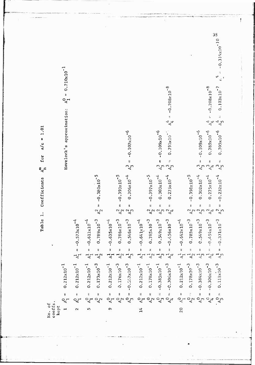
1. Coefficients A for a/c = 1.01 38 n
2. Coefficients Am for a/c = 1.02 . . 39 n
3. Coefficients Am for a/c = 1.06 40 n
4. Coefficients A for a/c =1.10 41 n
3 5. Wave resistance R/itpgc 42

mmmf^mtwrnm-r-r'^ m* **iß u
LIST OF FIGURES
Figure Page
1. Density of source distribution along a horizontal meridian plane near rear of spheroid (a/c = 1.02) 45
2. Density of source distribution along a vertical meridian plane near rear of spheroid (a/c = 1.02) 46
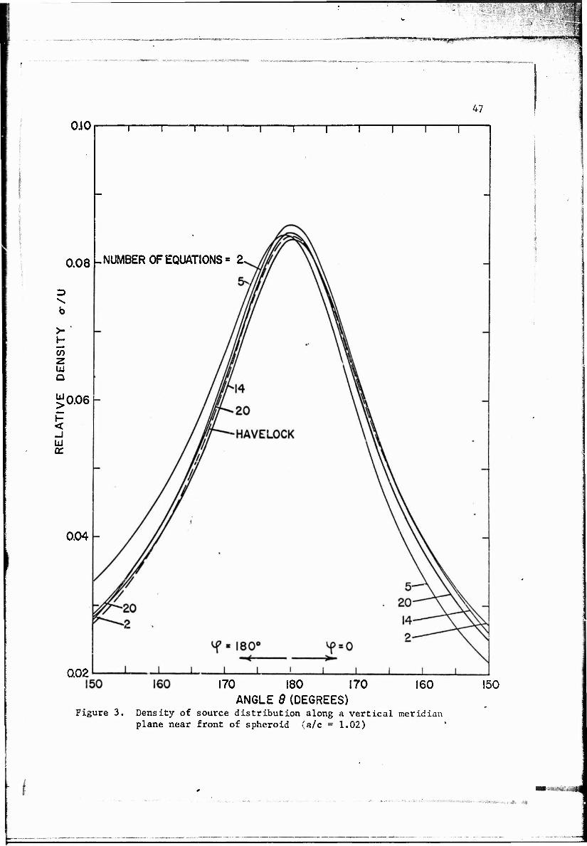
3. Density of source distribution along a vertical meridian plane near front of spheroid (a/c =1.02) 47
4. Density of source distribution along meridian planes of the spheroid (a/c = 1.02) 48
VI

1 I ■ I' "™w"1™ ji.iiiii.ii ü ..■niium.in1nnp>qi|Uii i ,I«VI,,»
INTRODUCTION
Even the simplest problems involving free surface waves are
difficult to treat analytically when formulated exactly. In dealing
with these problems, therefore, one must introduce simplifying assump-
tions intc the equations of motion and the boundary conditions, and
replace the original problem by a new one which is more amenable to
mathematical treatment and which should approximate the original one in
some prescribed way. If viscosity is neglected and irrotational flow
is assumed, the problem reduces to finding solutions of the Laplace
equation. The free-surface boundary condition, however, is nonlinear,
even if surface tension is neglected, and moreover it must be applied
on a surface of unknown location. As a result, further simplifica-
tions are still needed in most cases. For flows about submerged ob-
stacles, the assumption of irrotational flow may lead to a new problem
which does not approximate the original one; such is the case, for exam-
ple, with flow about circular cylinders and spheres, these two shapes
being very attractive to the mathematical researcher because of the
simplifications they bring about in the mathematical expressions.
In order to deal with the nonlinear free-surface boundary condition,
special approximation techniques have been developed. For flows about •
submerged bodies, these techniques transform the problem into a series
of linear problems with nonhomogeneous boundary conditions (with the
"'■■■'■"-■
exception of the first order or infinitesimal wave approximation, for
which the corresponding boundary condition is homogeneous), to be ap-
plied on the plane of the undisturbed free surface. Even within the
theory of infinitesimal waves, however, an exact solution is difficult
to obtain. An additional approximation is involved in many researches,
since the boundary condition on the surface of the body is not satis-
fied exactly. If one assumes that the shape of the body is such that
perfect fluid theory can yield results oE practical significance, the
determination of the errors due to the failure to satisfy the nonlinear
free-surface boundary condition on the one hand, and the boundary con-
dition on the surface of the body on the other, is of great practical
interest.
In the present work, the wave motion produced when a stream of
constant velocity is incident upon a submerged prolate spheroid with
its axis parallel to the free surface and in the direction of the
stream will be treated. This shape is of interest in connection with
the wave resistance of submarines; moreover, perfect fluid theory can be
expected to yield results of practical significance when applied to
determine the flow about slender prolate spheroids. The free surface
boundary condition will be linearized; the boundary condition on the
surface of the body will be satisfied exactly. Thus, an answer will
be provided, for this particular shape, to the latter of the two pro-
blems posed in the preceding paragraph.
A short summary of past researches dealing with the theory of
infinitesimal waves in flows about submerged obstacles is included be-
low. Only streams of infinite depth are considered.
M£M%nMR3 '.,>l«->-.™a

-
The first detailed evaluation of the wave notion caused by a fully
submerged obstacle is contained in a paper by Lamb (1913) in which the
disturbance produced in the flow of a uniform stream (of infinite depth) E
by a submerged circular cylinder is dealt with. The evaluation yields,
actually, the disturbance produced in the flow of the stream by the
dipole which generates the cylinder in an unbounded fluid. The boundary
condition on the surface of the cylinder is not satisfied and an anom-
alous moment on the cylinder results (Wehausen 1960, p. 576; see also
Havelock 1929). As Tuck (1965) has shown, no closed body is actually
generated. Thus, Lamb's analysis provides only a first step in the
solution of the linearized problem.
Let 0_ be the velocity potential of a uniform (unbounded) stream.
Let 01 be the velocity potential of the image of 0fi in the sub-
merged body; that is, 0.. is such that 0.. + 0.. satisfies the boundary
(s) condition on the surface of the body. Let 0 be the velocity po-
(s) tential of the image of 0.. in the free surface; that is, 0- is
(s) such that 0 + 0 satisfies the free-surface boundary condition
(s) and the radiation condition at x = -co. Let in general 0 be
n
the velocity potential of the image of 0 in the free surface and
(s) 0 ,, be the velocity potential of the image of 0 in the submerged n-t-l n
body. The sequence
<>o+ h + "i(s) + •••+*, + KM * <U + • • • •
if convergent, yields the complete solution to the linearized problem.
This program has been carried out by Wehausen (Weha.isen & Laitona
1960, pp. 574 et seqq.) for the case of the circular cylinder. In

[T '■ —— ^
this case, ß can be obtained fro« ?■ by iseans of a forauia of n u
(s) Köchin, and x? ., fron 2 by using MiLne-Theiason:s circle theorem;
TV^L n
Wehausen has shown the series re be convergent. Cylinders of other
shapes can probably be handled by a combination of this technique and
coaformal napping.
A complete solution frr the submerged circular cylinder was also
given by Havelock in 1936. In previous papers (1917, 1927, 1929)
Havelock had applied to this problem the method of successive images
later used by Wehausen to give a complete solution, evaluating the
second set of images within the cylinder and the corresponding image
in the free surface, and thus carrying the computations two stages
further than in Lamb's solution. In his 1936 paper, however, he used
a different approach and obtained the solution by expanding the complex
potential of the system of sources and sinks within the cylinder in a -n
Laurent series, £ A z , about the origin. The free-surface boundary
condition (and the radiation condition) can then be satisfied by adding
a suitable expression in terms of the coefficients A of the Laurent n
series, and the boundary condition on the surface of the body yields
an infinite set of equations for the coefficients A . The procedure,
which lends itself well to approximate computations, amounts to pro-
ducing the flow outside the cylinder due to the system of singularities
inside by placing at its center an infinite number of multipoles, mod-
ified to satisfy the free-surface boundary condition (and the radiation
condition), and whose strength is chosen so as to satisfy the boundary
condition on the surface of the body. Havelock found, for the wave
resistance of the circular cylinder, the expression

— ——' "■ ....--
•9W» ■*. * M ■_us>. -a- -rji
R = 4s plT(k a) e ^ l-2r.(ka)2 - (r,-3r.2+s2) (k a)4 + l o 2 1 O
•(
where a is the radius of the cylinder, d the depth of submergence of
its axis,
ko = g/U ,
s = 2se"a,
a = 2k d, o
1 r = —rr + 2
a
' (n-1)! (n-2)! . i •
i -a e li(e°) , )
and li denotes the logarithmic integral. The first term in this ex-
pression is that obtained by Lrimb for the wave resistance of the circu-
lar cylinder.
The approximate .. to the wave resistance of a submerged body which
is obtained by evaluating the flow about the singularity distribution
that produces the body in an unbounded stream has been calculated by
Havelock for the sphere (1917), for prolate and oblate spheroids aoving
in the direction of the axis of symmetry and at right angles id it
(1931a), and for an ellipsüxü with unequal axes moving in the direction
of the longest axis (1931b). Havelock evaluated the vave resistance of
the sphere by direct integration of the horizontal component of the
pressure on its surface; the method of successive iiaagns was applied to
compute the second set of images within the sphere, needed in order to
satisfy the boundary condition on its surface to the required degree
of approximation. The computation of this second set of images can be
dispensed with if Lagally's theorem is used to obtain the wave
>" ■—uaw —awteWl
■fOTI^T ■ —»»■ • -■
6
resistance to the same degree of approximation. This fact was noticed
by Havelock in his 1929 paper on the circular cylinder, in which a proof
of Lagal'y's theorem for the steady two-dimensional case in which only !
1 sources, sinks and doublets are present is given. The proof is based on
the Blasius formulas for the force and moment on a closed contour in
two-dimensional, incompressible, potential flow; the name of Lagally is
not associated with the result. To compute the wave resistance for the
spheroid and the ellipsoid, however, Havelock made use of a previous
result for the wave resistance of an arbitrary set of doublets in a .
uniform stream (1923; see also 1932) obtained using an artificial method
due to Lamb (1926). The method consists in making use of Rayleigh's
artifice of including a fictitious dissipative body force, -p^'V,
proportional to the disturbance velocity, calculating the energy dissi-
pation as
RU = u'P / 0^ dS
where the integration is taken over the boundary of the fluid, and
interpreting the finite limiting value of this expression, when p,' is
made to approach zero, as the rate at. ^hich energy is propagated out-
wards in the wave motion.
In his 1929 paper on the circular cylinder Havelock pointed out
also that the second set of images within the cylinder is needed if
Lagally's theorem is used to verify (to the degree of approximation
afford3d by the first image within the cylinder and the corresponding
image in the free surface) that the moment about the center of the
cylinder vanishes. Indeed, application of Lagally's theorem shows

■ ■ •'■'
immediately that a contribution of the required order of magnitude
arises from the interaction of the external uniform stream and the
second set of images. For a prolate spheroid moving along its axis,
the contribution to the moment arising from this interaction was calcu-
lated by Havelock (1952). The same task was undertaken by Pond (1951)
for the Rankine ovoid and later (1952) for the more general case of an
elongated body of revolution. Pond does not obtain the second image
system exactly. Instead he uses Munk's technique and obtains, witn
some additional simplifications, an approximate image system in the
form of a distribution of doublets along the axis of the body between
the limits cf the distribution that produces the body in the uniform
unbounded stream. Lagally's theorem yields then immediately the re-
quired moment. Pond's result agrees with the approximation that
Havelock, based upon his analysis for tte prolate spheroid, proposes
for long slender bodies of revolution.
The case of the fully submerged prolate spheroid, which will be
dealt with in this work, was treated analytically by Bessho (1957),
who tried to satisfy exactly the boundary condition on the surface of
the spheroid using a distribution of sources on it. Bessho considered
first an ellipsoid with three unequal axes and was thus able to use in
the solution of the problem several results on Lame's functions given
by Hobson (1931, Chap. 11). His final expressions, however, appear to
be incorrect, possibly because of typographical errors, and his numeri-
cal evaluations are rather inaccurate. In the present work, a more
direct attack using spherical coordinates yields an equivalent set of
equations for determining the source distribution, but with certain
«xaatmxuatxiiwnMiMsmti***msaswaawBaMEhaafr.
T
significant corrections. Furthermore, the numerical evaluations are
performed to a high degree of accuracy, avoiding the rough approxima-
tions employed by Bessho.

BASIC EQUATIONS
For convenience of reference the equations describing the
irrotational notion, under gravity, of an incompressible fluid having
a free surface are collected here. Derivations of these equations
can be found elsewhere.
Let Oxyz be a right-handed rectangular coordinate system and
let the y axis be directed vertically upwards. Since the notion is
irrotational, we have
v = V$ (l)
where V is the velocity vector and <p is the velocity potential.
Since the fluid is incompressible, it follows from the equation of con
tinuity that © must satisfy Laplace's equati
V2$= o
:ion
(2)
The Euler equations of motion, on the other hand, yield the integral
gy + £ + f - P 2 O;
where g is the acceleration of gravity, p is the pressure, p is
the mass density of the fluid, and t is time.
To these equations we must add the appropriate boundary condi-
tions for the problem on hand. Let S(t) be a boundary surface and
let it be described by F(x,y,z,t)=L. Since no transfer of matter takes

"^p^"
10
place across S(t), we must have at every point of the surface
ÖF ÖF ÖF OF Vx^ + Vy5y- + Vz^+Sf=0 <4>
where V , V , and V are the components of the velocity vector V.
At a fixed boundary, condition (4) reduces to
3n = 0 (5)
d/dn denoting the derivative in the direction of the outward normal to
the boundary. If
y = *f(x,z,t) (6)
describes the free surface ex the fluid, condition (4) takes the form
v i) - v + v *\ +*i =0 x (x y z (z (t (7)
Let p be the constant pressure above the free surface. Then,
in addition to the kinematic condition (7), we must have at every point
of the free surface
p(x,y,z,t) = po , (8)
since we neglect both surface tension and viscous effects. When use is
made of Equation (3), this condition becomes
g V2 . ö<
"1 + 2" + Sf=0 (9)
to be satisfied on y = />|(x,z,t), the additive constant having been
merged in the value of d^/dt.
In the following, the perturbation produced by a submerged obstacle
* ™*ws.*W»"ii«K*«W *•*•»«'

— ......y,.-..-. ■-. "' 'I-"""«.
in the flow of a stream of constant velocity U will be considered. It
is then convenient to write
9 ■ Ux + 0 (10)
where the perturbation potential 0 satisfies the Laplace equation
V 0 - 0 (ID
and to let u, v, and w be the components of the perturbation
velocity, that is
b0 dg M ox oy oz
The boundary conditions become
M=uöx + Ög=0
on on On
on the surface of the body, and, since the motion is steady,
(U+u) if - vrw»jr = 0
and
g"| + l((u+u)2 + v2+w2l 1.2
r = 2U
(12)
(13)
(14)
(15)
on the free surface y = *?(x,z).
The boundary condition that the velocity potential must satisfy
on the free surface can be obtained by eliminating "7 between (14)
and (15), as was done by Landweber (1964). It is more convenient, how-
ever, to proceed as follows. On the free surface
P(x,y,z) = p^_

•in.i ii pii
SHSW " Prw'-JJJW, ^Hi
and therefore
-WJ|W-
12
^=v.VP=o
Substituting p from (3) into (16) we obtain
gv + | V . V V2 - 0
(16)
(17)
This is the nonlinear boundary condition to be satisfied by the
velocity potential on the free surface. If we let
2 _ 2 , 2 _, 2 q - u + v + w
since
2 2 2 V = U + q + 2Uu
we can write (17) in the form
* ^ 9* 2 \ -9K ^ 22r j = 0 (18)
or, making use of (12),
u 2^ + 6li = Qr* 2
% 9\ Z [ QK QW 2>& (19).
to be satisfied on y = "^(x.z).
For a stream of infinite depth we also have as a boundary condition
lim grad 0=0
y ^ _ OO
(20)

i inn» Hi» in ■ '■ " ■ "i ■ 1 »»*^F"^^*WIIW^™^^t
- ■*-» ? .-.-*..'. r.,J^ —
13
that is, the perturbation vanishes far below the body. In addition to
the boundary conditions (13), (14), (15), and (20) we must also have
lim grad 0=0 (21)
that is, the motion must also vanish far ahead of the body. Thif; so-
called "radiation condition" need not be imposed if Rayleigh's artifice
of introducing a fictitious dissipative body force proportional to the
disturbance velocity is used (Lamb 1932, p. 399; see also Wehausen and
Laitone 1960, p, 479) or if an initial value problem can be formulated
(for which the boundary condition at infinity is simply that the motion
vanishes everywhere) whose solution yields the steady-state solution
sought as t—— oo (Stoker 1957, pp. 174-181; see also Wehausen and
Laitone 1960, p. 472, for additional references).
Although Laplace's equation (11) and the boundary condition (13) on
the boundary of the body are linear, the free surface boundary condi-
tions (14) and (15) are nonlinear. This nonlinearity precludes the use
of techniques of solution based on the principle of superposition.
Thus, the method of separation of variables and expansion in eigen-
functions cannot be used, and neither can the method of Green's func-
tions or singularity distributions. Moreover, the free-surface boundary
conditions are rather inconvenient because they are to be applied on a
surface of unknown location.
Under these conditions, special problems in the theory of surface
waves have been treated by using approximation techniques (actually
perturbation procedures) of which a fairly complete account has been
«-***--;.--- :■ -^sn- S ■'■'■■■ -. m ■" .-\^4Ü

14
given by Wehausen (Wehausen and Laitone 1960). Since only the first
order approximation will be treated here, the perturbation analysis
applicable in our case is r,->t included and the reader is referred
to Wehausen's treatise for details of the method. The first order
approximation consists of neglecting all second order terms in the
free-surface boundary conditions and applying them on the plane y = 0
instead of on the free surface y = ^((x.z). Equations (14), (15), and
(19) become, respectively,
U"7 - v = 0 (22)
g "*J + Uu = 0 (23)
and
U2^ +j2*-0 (24)
to be satisfied on the plane y = 0. Equation (24) can be obtained
directly from (22) and (23) by eliminating "7 between these two equa-
tions.
It is interesting to note the boundary condition that the second-
order contribution to the perturbation potential must satisfy. This is
_ U i-1 w f\ Z
(25)

-..-■■■-■ ■■■:----i >,
15
to be satisfied on the plane y = G. Once the first-order approximation
f(D is known, therefore, the second-order contribution .an oe obtained
by solving another linear problem with a nonhcmogeneous boundary con-
dition on the plane y = 0.
mmmn^/Kfm H --.-..

'S»»« ■PS*^—at --^F*«w*r«**
16
ANALYTICAL TREATMENT
The solution will be sought in the form of a distribution of
sources on the surface S of the spheroid. The determination of ehe
surface density a of this distribution is the object of the follow-
ing analysis.
Let the x axis coincide with the major axis of the spheroid
situated at a depth d below the free surface. Choose the y axis
vertical and upwards and let the origin be at the center of the sphe-
roid. Let the stream, of constant velocity U, flow in the positive
x direction. The velocity potential corresponding to the three-
dimensional motion past a unit source at (^,*],*S ) is given by
0s = Ux -j + G(x,y,z;^,^t^) (26)
where
2* ,o© b+kp met -H^'l) k- ko stc^t"
-t. ^
K ,2.
2l<oL I Sect -JT
y < 2d - "7

■
17
* 2 Here Re denotes the real part of a complex number, k = g/U , g is
the acceleration of gravity, and
R2 - (x-5)2 + (y-"])2 + (z-$)2
The harmonic function G(x,y,z; 5,, "1 , ^ ) is sometimes called the
Havelock potential since Havelock (1932) was the first one to express
it as a double integral in terms of Rayleigh's fictitious viscosity.
We have then for the velocity potential Cp corresponding to the dis-
tribution of sources on the surface S of the spheroid the expression
$ = u*~i&T^>iv+s+j^w^N,*;Ki,y}^ (28)
y < 2d - b
where 2b is the length of the minor axis of the spheroid and the
integrations over the surface S of the spheroid are performed ir»
the variables J, , "| , and ^ .
Since (26) satisfies the free-surface boundary condition, the
boundary condition at y = - 00, and the radiation condition at
x = -00, so does the velocity potential <p given by (28). The
unknown surface density a must therefore be determined so that the
boundary condition the surface of ehe body,
§1-0 dn
The symbol Rft could be left out since the imaginary parts of the two expressions within brackets are identically zero.
««««■MSIW»*»«»»«^**»«^^^ j , ^_

rison!«» r
18
is satisfied. YJhen (p , as given by (28), is substituted into this
boundary condition, a Fredholm integral equation of the second kind is
obtained for c,
ZTTXH^ITAJ-I 7> ! <rU7,*)+| ^V/,V)~j-^ * ^(x(g^;^^)U{5 «-UÄ (29)
The solution of this integral equation will be sought by expanding the
functions involved in series of spheroidal harmonics, thus taking ad-
vantage of the particular shape of the body.
On changing the order in which tha integrations are performed, we
can write <p in the equivalent form
$= ^-/^V?/^4-1* 2TT °0 , .
ZKl J it-/to Ac21"
-r
4^at-
^ /2 _, -^k^l sect k0sectr[ y + i{^^t+2^i)l
lie .2
I (30)
We will denote the length of the major axis of the spheroid by 2a and
its focal distance by c. Let "1 , &, and <J> be the orthogonal con-
focal coordinate system defined by
x = c cosh f) cos G ,
y = c sinh "1 sin & cos ip , (31)
; inh f\ s in 9 s in ^J . z = c s:

~
19
Th surfaces "7 = constant are confocal prolate ellipsoids of
revolution, with common foci at the points (+c,0,0). The surfaces
0 = constant are confocal hyperboloids of revolution, with the same
foci. Let 'A be the value of the confocal coordinate rt1 that I corresponds to our spheroid. We have
a = c cosh fl , b = c sinh "? (32)
Let £(9 ,(P) be the value of the Newtonian potential
on the surface of the spheroid, and let it be represented by a series
* of surface spherical harmonics,
Hobson's notation, which is also the one chosen by the National Bureau of Standards in its Handbook of Mathematical Functions, is used in this work. We have
m _ 2 dmP (z)
P (z) = (z -1) — , n . .m (dz)
m 0 2 d
mP (x) P (x) = (-1) (1-x ) » n , , vm (dxr
m ,m„
2 d'"Q (z) m, N , l . n Q (z) = (z -1) —
(dz)
m 0 2 dmQ (x)
Q (x) = (-1) (1-x ) — , n , . .m
(dx)"
where z is any complex number not roal and between -1 and 1, x is a real number in the interval -1 < x < 1, n and m are positive inte- gers or zero, m < n. The only points of discontinuity of the functions Pn'(z) (m i- 0) and Q™(z) are on the straight line (-1,+1).
^■■.^?;:v..,.,4H*1:,t;;iM,;;:.. . . ,.,-.. . , .... ; ...

20
co
We assume this scries to be absolutely and uniformly convergent over
the surface S. We can then write (Hobson 1931)
(33)
this being the potential function for the space external to the spheroid
which converges to f(0,-,) on the boundary. For the potential func-
tion for the internal space which converges to £(@,<^) over the
boundary we have the corresponding series expansion
OO M
£?>*») <*«f ?"(**fl (35)
The surface density a can be expressed in terms of the coefficients
a of these expansions. We obtain (see Appendix A)
Ov rtt AV1-H
a- = U Y V A M. S C°'-°} <■* •».£ x (36,
where, for convenience, we have put
A["m a~ i-ttlL ! (37,
I
u.'HH»'1 ,. 11 ixwM—"»y
mwin»- -;s-—'- ^"-w "->-'."~rti?**ii£3fiÄrai->2ff w~J;^fc:v^.^>-.<-tr~:W;r--«^^^<s=#^re*^s--r-4"WP
21
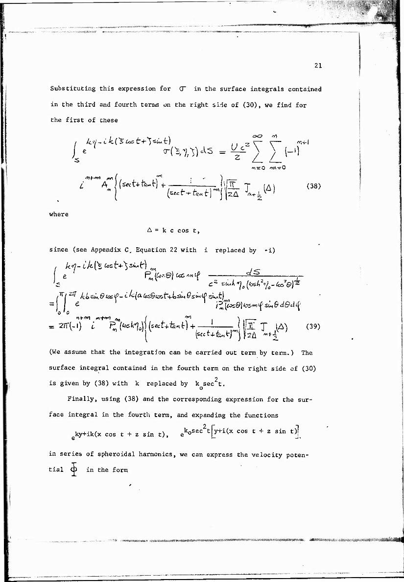
Substituting this expression for CT in the surface integrals contained
in the third and fourth terms on the right side of (30), we find for
the first of these
k'fl - i k ( ^ Cos t+*) *ü* t) OO r/\
(\iiv^ = "T-~\ 7 M ifi-i-i
I =: 0 rfA ■= C
^JLT IA)
where
t+fe-frfV L_ | (««*•■*■ few tPjjzÄ "Wl
A = k c cos t,
(38)
since (see Appendix C, Equation 22 with i replaced by -i)
cA' c2 *u-A -^ (4«/,ZYO-6/©)*
0 '0
= 2'T(-') £ % Mt)1 (^t+fe^ 0 + ! 1 |JX J (A) (39)
(We assume that the integration can be carried out term by term.) The
surface integral contained in the fourth term on the right side of (30)
2 is given by (38) with k replaced by k sec t.
Finally, using (38) and the corresponding expression for the sur-
face integral in the fourth term, and expanding the functions
ky+ik(x cos t + z sin t), ekosec2<:|y+i(x cos c + z sin o]
in series of spheroidal harmonics, we can express the velocity poten-
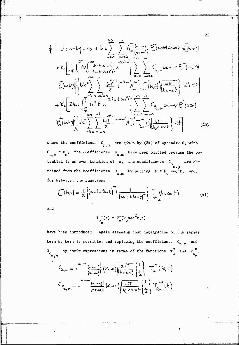
tial <p in the form
«»»»«»»'ssm*«»«»»!»«»» 'iKmmmsmmmt.t^fmmäii*iiiM^!':ir-':'iMiäii!d
I
22
v— ^— %-i
/v|=0 flftlssO
^ f2tr l°°L L *h -zk^(V
— , 2ff ,oo
2TT »1S.O /VK-O
X. •+- ^c
»*l
Z^ot
•> IrO OKI =0 "7/ ?/ OO O/l
3- 2
2 I m s O <wi —O
^MTIIIW«-') )f-i A„, i.i(« /W=C> »Wi'*o
dt- (40)
where tha coefficients C are given by (24) of Appendix C, with
C = C , the coefficients B have been omitted because the po- tt,o n n,m r
tential is an even function of z, the coefficients C are ob- n,m
tained from the coefficients C by putting k = k sec^t, and, n,m * r & 0 > »
for brevity, the functions
x^i^k^M* (s*ct+62*.tT'H -vt-l
] T [kttet) (41)
and
T m(t) = Tm(k sec2t,t) o no ' ' n
have been introduced. Again assuming that integration of the series
term by term is possible, and replacing the coefficients C and n,m
C by their expressions in terms of the functions T and T , o J r no' n,m n
-o

«w»
23
we can write (40) in the equivalent form
.»»I +Uc2 2_ ^tes9)60 *«© ^so ,
oi'rO'»"'=0 CO "» f \ I —
• 0 t A I -t
z "Y1 Mt
where the factor 1/2 is to be used for m = 0. Substitution of this
expression for the velocity potential into the boundary condition on
the surface of the spheroid,
. ai £§»
yields
^s~ = 0 or T?7 = 0 on 0"7
Oo Al OO ^
Kl +/W1)
7 (2 ) ('*■*-'*»)' (*. if x ' v£
*1 = 0 /»»=0
AH ( I ] , v| __ « + "•*
«i~0 nri = 0
I-') ' <1, Avl (^vi I
(H 'i O "H'» O
-IT £a5 f— ^"^.w^ = 0 (43)
- /""WSB*lftwi'-,mteii8BflH$jH5H|M

"T ■ I MM
24
whera we have now assumed that the series can be differentiated term
by term; the dot above the Legendre functions P and Q indicates
differentiation with respect to the argument cosh »\ . Equation (43)
is equivalent to the infinite set of equations
t*\ n\ \~ \— i* ft ml
A « r + ) ) 8 A (44)
where
"1 =0 P* =rO
,flv\
•~ —\
0
if n = 1, m = 0
otherwise
and
B , = °- ^ M . 4.I2-.M) i-o I
with
/nt__«n
I, = (n+m+n' +m') even
2, )twt^V<wVl H _2i^oct s*e C"
I-') o &Ä£
(n+m+n1+m') odd

' i
WJ
25
CALCULATION OF THE WAVE RESISTANCE
Lagalxy's theorem (Lagally 1922) yields for ehe norizontal component
of the force on the spheroid the expression
(45)
where 0 is the Havelock potential for the source distribution on the
surface of the spheroid, given by the third and fourth terms on the
right side of Equation (3C). We have
T^lL d: = Ze s-X 27T/ K- - ka "S<cb
\
•4- %
2. o -2 kn £ s«c t
Zk<- I 5&t L_ Lrr
2.
(46)
where both surface integrations are performed over the surface of the
spheroid, in the variables x, y, and z when we denote it by S, and

' rt'?^: • ;.>ff^gg'W IMI üfOfC^^teM-^-TWJ^gV*»^' -^~- ,.^xr,B5':-;:?; ■- ft;-"' :' : S5MS«
26
in the variables i. , ^l , and Y when we denote it by S'. The
contribution to the wave resistance from the first terra on the right
side of (46) is zero. To see this we need cnly write
s k)j+Lk(xCoct+ xrSUt irj
Afjtijl 7' r
s s-
and observe that if we interchange x, y, z, with "S , *7 , \ , the
integrand changes sign while its absolute value remains unchanged. To
evaluate the contribution to the wave resistance from the second term
on the right side of (46), we make use of (38) with k replaced by
k sec t. We obtain o
94* <r ." yg eis = ^ 0* 7i
2.
zrr _- ifrr "»*."■'<""'r'f^r rrA\, r\~" -.+1
A £ j The wave resistance is then given by
oo ^ CO
X«ir(j ,+-/>,' rt* rtw' OT «X
(r>) A« A„, J^,
/*f=0 «|:D ">'=© AV)'=0
(n+m+n'+m') even
(47)

» »■*&■'» IT» ■■I*J<^'»«—^Jg^gg-*~WMIW XHerqgßnmmf WPW
27
where
lfin4»V <-.«-•
fVl /»!< = H ^7T sec r-e ** *—'
■x^-m^^.^i-.,.

r ^pm^pqpgm gvvMVfN
28
NUMERICAL .'VALUATIONS
All numerical evaluations were performed with an IBM 360/65 com-
puter. The corresponding programs car be found in Appendix E and will
be discussed in this section. Subprograms which are common to various
programs appear only once in the Appendix.
In order to evaluate the single integrals in the coefficients of
the infinite system of equations (44), we introduce the change of
variable
tan t = u.
Let
I. = «T 5 -2k0Ä seczir
(2. —*0<
Cast T0 fa To & -It (48)
We have
X -ikA /~ -ZkAu2-
<?*| e \JTM7
1
where
(49)
Since the integrand in (49) is an even function of u, we can write
■zkA I, ~-STT
■fiJ^l 2]( CLK,
HJzMJ
(50)

29
where we have further changed the variable of integration to
x = \| 2k d u o
The integral in (50) can be evaluated by Hermite-Gauss quadrature. A
twenty-point formula was used, for which the zeros and weighting factors
can be found in Abramowitz and Stegun (1964). Actually, since the
integrand is an even function of x, only ten ordinates are evaluated
in the corresponding c mputer program, which yields the value of I.,
and includes a function subprogram (BSSSJ; to evaluate the Bessel
functions which appear in the integrand.
The evaluation of the Bessel functions J of order n + 1/2 was
carried out using the series expression
(51)
for values of the argument less than five, and the recurrence relation
T (?) = _ J (52)
for values greater than five. In this manner, the large round-off
errors associated with tbe use of (51) for large values of the argument
(especially for small n), and with the use of (52) for small values
of the argument, are avoided. The cut-off value of five is a rough
estimate of the value necessary to minimize these errors. The sub-
program, which was written in doubl' precision further to reduce round-
off errors (only six, or at most seven, significant digits are supplied
by the IBM 360/65 computer in single precision), was checked against
. - **^.^.*a*w*um#r**m*****wt i iwnitii null Hiai^HrtHlHitfililiiiHÜIH^

30
tables included in Watson's treatise (Watson 1944, pp. 740-743). The
results were found to be accurate to the number of significant figures
given in these tables (six or less) for values of n up to 18; most
of them are probably accurate to several more significant figures- The
round-off errors associated with (52), however, increase with increasing
n, and this high accuracy should not be expected to obtain in the eval-
uation of Bessel functions of much larger order.
"in view of the difficulty of estimating the error in the Hermite-
Gauss quadrature formula, the calculations were spot-checked using
Simpson's rule, which requires longer computing times, but allows for
a ready estimate of the error at each stage of aprroximation. The sub-
routine SMPSN used in the corresponding program is part of the IBM
System/360 Scientific Subroutine Package, Version II, and is not in-
cluded in Appendix E. In this subroutine, Simpson's rule is used with
interval halving until the difference between successive values of the
integral is less than a given tolerance. The Hermits-Gauss quadrature
formula was found to provide at least five significant figures.
To evaluate the double integrals in the coefficients of (44), we
make use again of the change of variable
tan t = u
and we put further
k = k K o
Let
^. H r>v( ^^"'Z f-z T>,«CM dkdt (53)

^^™
■w
31
We have then
oo o=< -2A-c[k
I. /* /o K-(l + v*} fOJU-u* ( [\ri+^ + u)""j
M.^* fll+«**UJ + ty+l
For numerical evaluation, it is better to write (54) in the form
(54)
kaC 0 ll VT^j r
~-^AI+/»1 +2-/
H-W
14- VlM
If fü-
-2MK •e
/»4-m1 -p , k0cK\ j fifo(Kj ] =>o
(55)
where the function
X.+JA») I "i+-t /«•*-4r
I -_2 4- ... , (56)
is continuous at z = 0. A simple modification of the function sub-
program used to evaluate the Bessel functions yields the function sub-
program (BESSJM) used to evaluate (56).
The evaluation of the Cauchy principal-value integral in (55) was
»••wa«aeuMKtMW«K33igMciamM Ää|fe*k*4''

T 32
carried out using Simpson's rule, modified according to a technique
suggested fay L. Landweber (Kobus 1967, Appendix 1) to take into account
the singular point in the integrand. It can be shown that any composite
integration rule, obtained by dividing the interval of integration
into subranges and applying in each subrange any of the Newton-Cotes
integration formulae, can be used to evaluate a Cauchy principal-value
integral,
,b
-^ dx, a < c < b
as long as the singular point c is either an end point (excluding a
and b ) or the middle point of a subrange, and the value of the inte-
grand at c is taken equal to the derivative f'(c). In the function
subprogram that evaluates the function G(u) defined in (55), there-
2 fore, the derivative at the singular point k = 1+u is obtained first
using a five-point differentiation formula. The two function subpro-
grams FM and F evaluate the integrand of the principal-value inte-
gral and, at the singular point, replace the integrand with the corres-,
ponding derivative. The calculations were carried out to an accuracy
of three significant figures.
The solution of the infinite system of equations (44) was obtained
by using the so-called method of reduction (Kantorovich and Krylov 1958,
pp. 25-26, 30-31). In th.is method, the solution is found by solving a
sequence of finite systems, each of which is obtained from the infinite
system by discarding all equations and unknowns beyond a certain number
N. The solutions of this sequence of systems, under certain conditions,
converge to the (principal) solution of the infinite system. Although

1
33
it is difficult in our case to show that the conditions of the theorem
are satisfied, it is reasonable to assume, on account of the significance
of (44), that the method does yield the solution sought. A numerical
verification of this assumption is obtained if, when the number N of
equations kept is increased, the coefficients A approach limiting
values.
Such a numerical verification has been included in the computer
program for the solution of (44). The number of equations has been
taken equal to 2, 5, 9, 14, and 20, equivalent to keeping, in expansions
(34) and (36), only those terms containing Legendre functions of degrees
up to 1, 2, 3, 4, and 5, respectively. The program contain.: a sub-
routine subprogram for computing the coefficient matrix B , from the
symetric matrix formed by the double and single integrals I . No n n
table was found to give the values of the Legendre functions and their
derivatives in the interval of interest to our work, and their evalua-
tion is carried out in a second subprogram. The derivatives occur in
the coefficients B , ; the Legendre functions of the first kind in n n
expansion (36). No use is made in this second subprogram of the re-
currence relations for the Legendre functions, on which, for example,
the tables published by the National Bureau of Standards (Lowan 1S.V5)
are based; severe round-off errors were found to be associated with the
use of these relations, in particular near x = 1.' Instead, since only
the functions of deg>es up to five were needed, the explicit expres-
sions of these functions were derived and used in the computations.
These expressions were checked, using the National Bureau of Standard
tables, for several values of the argument; all significant figures
!*'.-■». *.l ifÄüKV "i ■ '■•>.'."! ^^*».-i.*vi«^w^w,;..,.Si!.i;.j1,Aarfl1l w ^ & ^r*«*T * t nK t ;■,... :,.■ ',,

34
given in the tables were found to be correct. The subroutine GELG
used in the program for the solution of (44) is part of the IBM System/
360 Scientific Subroutine Package, Version II, and is not included in
Appendix E. In this subroutine, the solution of a system of general
simultaneous linear equations is obtained by means of Gauss elimination"
with complete pivoting.
Once the coefficients A are known, we can evaluate the density n J
of the source distribution making use of (36). A program was prepared •
to obtain plots of this density along meridian curves of the spheroid.
The subroutine PNMXG1 used in this program, which evaluates the
Legendre associated functions of the first kind for values of the argu-
ment greater than one, is simply part of the subroutine LEGF; the
subroutine PNMXL1, which computes these functions for values of the
argument less than one, was obtained by introducing the necessary
changes in sign in the expressions in the subroutine PNMXG1. Neither
subroutine is included in Appendix E.
The evaluation of the wave resistance is carried out in the 3«ist
program in Appendix E. A simple modification of the program for the
evaluation of the single integral in the coefficients of (44) yields
the program for evaluating the single integrals in the expression (47)
for the wave resistance: the modified program is not included.

OliWWW*r,"'*S" *-**#««■*£**-'-•: r i?*y»>-C?l III! III UWIMH ' WJlUlll!<^ai
35
RESULTS AND DISCUSSION
The double and single integrals I . in the coefficients of n n
system (44) depend on the Froude number U/\ 2gc = 1/V 2k c, and on 11 o
the relative depth of submergence d/c, and are independent of the
eccentricity c/a of the spheroid, which occurs in the derivatives of
the Legendre functions. This property of the coefficients of system (44)
is of interest because most of the computer time required in order to
evaluate the coefficients A is spent in the evaluation of the double n
integrals; once these integrals have been computed, for given values of
the Froude number and the relative depth of submergence, the coefficients
A can be obtained for several values of the eccentricity without n '
practically increasing the total computing time. The numerical evalua-
tions reported here were carried out for a Froude number U/\ 2gc = 0.4,
a relative depth of submergence d/c = 0.5, and reciprocal eccentrici-
ties a/c = 1.01, 1.02, 1.04, 1.06, 1.08, and 1.10, corresponding to
slenderness ratios a/b = 7.12, 5.07, 3.64, 3.02, 2.65, and 2.40, re-
spectively. (For the relative depth of submergence chosen, the spheroid
pierces the free surface for a/c =\jl.25.) The practical interest of
the smaller slenderness ratios is probably limited; they are included
here for purposes of comparison and discussion of results.
The first approximation to the solution of system (44) which con-
sists of neglecting entirely the infinite series on the right side, thus
.-»^ees*»«»^»««»^**^

-^>^^^^,^--i--^^7^yi*r^t^v<>^^'^^nf^>^^i7nitw^^'r^.r,^r'^ -
keeping only the first term of expansion (34) with
36
a..
u fll® A°,=
C [& rj a/c _ _L L gV£±J Ka/cf~\ z ^c~l
(57)
corresponds to the source distribution that produces the spheroid in an
unbounded uniform stream without a free surface. Indeed, the potential
for the motion of a prolate spheroid parallel to its axis (in the nega-
tive x direction) in an infinite mass of liquid is given by
or f = u
Ü c
'p
Q&
P(fese) Q\«*L«I) (58)
with ^ = cosh »7 = a/c, ) = coshfl , u = cos 9. For this first
approximation, the wave resistance is given by
o'- f'Z -Zk0cL^C( Tp q C*"j'A, ) <iTf *«?<-€ J, (Ail c(f- z~Tqcs[A:f I'iv^e/j (59)
Equation (59) was obtained by Havelock (1931a) using the axial source
distribution corresponding to the motion of the spheroid in an infinite
mass of liquid and applying Lagally's theorem to evaluate the wave re-
sistance (without, however, mentioning the name of Lagally in this

ggyggSwaT"-?" fimim^n l'PWIJJW<t»IV"";^,-j«gi<«^a:^-««^CT-w- 5k -■«■gllH—«—!»■Ml I- I 111 ™W»M«Jj|B
37
connection). Of course, neither the axial source distribution nor the
source distribution on the surface of the spheroid actually produce a
spheroid in the presence of a free surface. They are two different
first approximations. It is interesting to note, however, that both
first approximations yield the same value as a first approximation for
the wave resistance. Havelock's approximation has been included in
Tables 1 through 5 for purposes of comparison.
The values of the coefficients A , obtained keeping 1, 2, 5, 9,
14, and 20 equations (and an equal number of coefficients) in (44),
are presented in Tables 1 through 4, for four values of the ratio a/c.
Table 5 contains the corresponding successive approximations to the wave
resistance (the two additional a/c ratios investigated are also in-
cluded in this table). Three significant figures are given for all
elements in the tables, since the double integrals were computed to this
accuracy. When 20 equations are kept, 92 double integrals must be evalu-
, , , . , m_m . - . , m,m m _ m ated (the integrals I , satisfy the symmetry relations I , = ,1
nn J J nnnn
and num m T m I ,, and this reduces the number of double integrals to n n n n
be evaluated from 202 to 92); the required computing time is a little
less than two hours. The corresponding computing time for the evalua-
tion of the single integrals is less than half a minute; for the solution
of (44), for the six ratios a/c investigated, including the evaluation
of the derivatives of the Legendre functions which appear in the coeffi-
cients of the system, less than one minute. Also less than one minute
is the computing time required for the evaluation of the wave resistance,
using (47); only single integrals appear in this expression. A reduction
in the time required for the evaluation of each double integral, at
: I
o I
38 o i—i
3
':■:
o 1
o 1—1 CM
o II
O i-l <
1 c
o X
CO cc
II
Ü
CC
SH
o
Vs
M u c a
•■-I o
•r-l
<4H
m
8 o
CO
E •H
o w a n.
u o i-i at >
i o
. i-H
o oo CO
o I
CM CS1 <
X r~- O i-i * O i
II
co co <
m <s
o o i-i rH
X X CO <J- OS o CO co • • o
1 o
II II
CN CM CN CO < <
I c I—I
X as o
<
o r^
co co co co < <
X X X r^. CO '1-1
cs O r>- en CO CN * • • o
1 o o
o I c x o
o 1 q x cs
CC r»
en co en
vO 1 o rH X in c r--
CO IT) <
O O
X X X X a;. CN in CM ON o r^ co CO co CN CN
CN CM CM CO CN <|- < < <
CMcMCMrrsCMvH-CMin < < < <
rtj H
■o- «tf CO ■•3- CO CO <t CO en CO <t CO co CO co
'o i o
i o O o O "o "o o o o O O O O
rH 1-1 r-i r-l l-H rH i-H rH rH rH i-H rH i-H i—i i—i
X X X X X X X.. X X X X X X X X CO 1-1 OS in vO vO i-H m CS vO CN in as <3" i-H
!>. r-l 00 CO 00 <t- <f CO «tf m <j" oo «tf m CO
in VD r^ o r~. m VO r» in vj- vO r^. in <j" CO
* O i
O 1
o o 1
O o c 1
c o o i
o 1
O ü C' o 1
II II II II II ll II II ll il II ii II I! II
<-H 1-* i-( l-H l-H CM l-H rH l-H CN r-l CO r-i r-i rH CM i-H CO *-* <f rH rH rH CM i-H CO "-t-tf rH \j-\
< < < < < < < < < < < < ^i < <;
rH r—i r-l en r-l en CO rH rH l-H en rH CO CO CO CO
1
o 1 o
1 o 1 o o O O o o O o O c o o "o
rH p-i 1-1 ■—I r-l r~l i—i rH rH rH I—1 rH 1—i rH rH . l-H
X X X X X X X X X X X X X X X X CN <N IN CO CN '£1 r-~ CM CO m o CM OO «* v£> ,-H
>-l iH rH r~- i—l r~ i.Z l-H r- CO o rH o. CO o rH
CM CN <N i-H CM l-H n CM rH CO CO CM rH CO CO rH * • * • • • » • • • • O o o o o Q o
i o o o
1 o
1 O o O
I o
I o
ll II 1! II II II ii II II !! II II II II 11
o ^ o <-* O I-* O CN O l-H O CN O CO O i-H O CM O ro O-tf O rH O CM O co Csf O LO • < < < < < < «3j < < < < <c < <5 < <
iw w ■
O a i—i CN en OS <r o • a a rH CM
o o ^ £5 a

i i. X .
«■■«=
CM o
o
O
V
•H O
IM 0) O
X vO ri vT • O
I
o -* <
c o
e •H X o M C c
u o
r-l
I I o I-l
X CM m co
■ o i
■ o
co • o i
IT» I o I-l
X CO i-l CM
d.
en n
CO I o 1-1 X
vO vO CM
■ o
o ov
V i o i-i X
co CO
IT) I o .-I X
C"v i-l CM
O
CO FO CO "d-
<; <;
i o r-l
X r~ oo CO
CO i o .-i X n vO CM
CO I o I-l X
CO r* CM
39 00
1 o -* X
r-* r-l
CO * o
1
ü
m m <
r^ vO
o o I-l I-l
X X •1-» vO o vl- ON vO • • o
1 o
II II
•sTsr ■vf U1 < <
IO vr -tf o o o I-l T-i l-H
ä X 00
X VD
CM CO *Ni" CM 1-1 I-l • • • o
1 O o
II II II
CO CO CO>J CO in < < <
1 CO
1 CO
1 CO
1 o o o o I-l t-l I-l r-l
X X X X 00 CM CM 1^ CO vO r-- o\ CO CM CM I-l * • • * o
1 o o o
1
CM
0) r-l
H
co i o I-l
X m CM
d i
CO i o
oo CM
CM CM
CM t O
o
CO
CM CM CMPj
CM I o
X X <* vO •tf o co co CO
X oo VO CM
CO
CMCvl CM CO CM -tf <; <j <;
X CO i-i CO
CM I O i-l
ä CO CO
CM I o r-l X
CM I o X
oo r- O CM CM
CMCM CMC0 CM-d" CM m < < < <
CO I o 1-4
X
CM I o
CM CM CM I I I o o o
X X XX ov i-i vo m
'co r^ o oo CO CM CM r-l
o I
o o 1
o I
o I
■HriHN rl rlrl N HI«! HrlrnNHflH^ rlrl HN HtO H<f H Ifl <<■■<<<! < < < <& < < < < <
A c-l r-l co 1 o
I-l CO CM I-l CO I o
CM 1 o
CM r-l CO CM CM CO
o o o o o o o o o o o o ' o I-I l-l r-l I-l r-l 1—1 1-1 1-1 r-l 1-1 I-l 1-1 i-l i-i ■ r-4 r-l X X X ä X X X X X X X X X X! X X
CO CO CO CO m CO r»- 00 —1 CO 00 CM o CM •* <r <t <f <* 00 oo ■* Ov oo r-- *tf a\ 00 !"*- CM -* ** •* 00 «* oo !-< >* oo 1-1 i-H >* oo ■-I 1-1 m o o o o o o o
1 o o o
1 O
1 o o O
i o
1 o
Oj* c < m 01 o IW u
m a r-l • CD w o O a. 2 O
V CM
© r* o CM o H ON on o r* o CM ono<* orHocMOcoo<j-om < < < •< < <!'<3 <; < <j <;<;,,<: •<
m CM o CM
mmx^™M-*^,im.aex«w,m>jmwMMmmimimmiM-if' .^ lMtr ,

40
st
o l
g
St I o
<3\
' i o I-i X
c* i-H i-H • o
1
II
m m <c
st n
o o r-4 ■-i
X X CM •-i OV m r^- f-i
o o
B
o
6
V
C
u 1-4 <w
<u o u
co
■3
a
8 u a
AS o o
1-4 <U
I
CM
O i-l
CM
d i
CM I o r-i
00
o I
eg CM
CM 1-4 I I o o 1-4 r-l X X m rH o m m st
ro i o i-i x
CM
st o ■
COCO
CM CM I I o o 1-1 1-4
ä & m o CM o\ • * o o
CMCM CMCO
CM i-H r-4 CM
O O O O 1-4 i-4 r-4 1-4
X X X X I-I a» CM o o o o st r^ st <o i>.
<•«* <
co CM i I o o I-I r4
X CM ä o CM m i-l • • o o ■
ii II
COCO CO-* < <
CM CM r-i 1 1 1 O o o ■-I I-I I-I
X X X r-4 m vt VO o r>. CM oo r-l • • • o
1 o o
II II II
CMCM CM JO CMst <J < <
X CM CO CO
X oo CTi in
X vO CO
st st vt m < <
CO CM CM
o o o I-l 1-1 1-1
X X X o CM Is» o r-l o in i-l co
o
COCO co <r co m < < <
CM CM r-l CO
o O O o 1-1 i-l i-l 1-1
& 3 X st
vO 00 V0 i-i CM r~ i-i i-l • • * ■
O 1
o r o
CM CM CM CO CM st CM m < < < <
CM I o r-l X
o-v CO
X vO r- CO
m oo m
CM CTV r-l St
O I
II
IH r
o
II
o I
i-lr-l r-ICM r-ICO
o i
o I
o I
o I
1-4T-4 i-ICM i-ICO 1-4 St < < < < r-i t-t i-l CM r-l CO r-l St i-4 lO <J < < < <
r-i 1-4 r-l I-I r-l r-l I-I <H rH CM 1 1 1 i 1 1 i 1 ' 1 o o o o o o o O o O r-l r-l 1-4 r-i . i-4 r-l 1-1 r-l 1-1 r-l
m m vO A vO X
VO £ VO £ 3 £ vO X X
St X X
VO m m m ■£> m CA CO m c\ o CO m o ON CM CM i-i i-i r-l r-l r-l r-l CM 1-4 1-4 CM St r-4 r-4 r-l St t~~
o o o O O O O 1
o o O 1
O I
o o o 1
O 1
o
»4-4 CO O «4-4 4J
«4-4 a. • a> 0)
o o x S5 o
V V CM
OH OCM OH OCM oeo OH ON On Ost
m o\
0:-4 ocM oco ost o m
o CM

■DP
41
ii
o «a
u o
V
c <D
•H Ü
•H '4-1 VH <U O
■s
o r-l X l-l o
o I
COCO <3
CN
O i
CNCN <!
X CN CTi CN
O rH X
CN vO CO
O I
o I
II
r-l
O
II
CNCN CNCO
VO CN <f CN in -* m N n
CM
O rH
X o\ 00 CN • o
1
II
•*.** <:
CM CM
O O r-l r-l
X X 00 CO CM CM 01 m • • o <J
1 . i
II II
COCO cost < <:
H CM
o o r-l r-l X X
CO >d- sf v0 e>- r-l CN CM r-l
CNCN CM CO CN»* < < <
X X I"» oo o r^. r-l r^ St VO CM
Sl- av
CO I O rH
X r~ vO oo o
1
II
mm < *
• CN CM
O O I-l r-l X X
o- o 00 CO CN CO
o 1
o 1
II II
st<r <*■ <n < <:
•J CM r-l
o O O r-l r-l r-l X X X
1/1 CO o o <f o OV U1 CO
COCO COvt- CO IA
o X X
VO CO CO CN in CN O CM CM St- rH r-l • * • • o
1 o o o
CM CM CMCO CNSf CM "*>
r-l I o
x in vo «*
X vO in vo
m vo m vo CM r-l
o i
o
II
o I
o I
X CM (O VD
O i
r-lr-l i-ICM i-ICO <! < <
rHr-l rHCM r-l CO rH Si" riH r-l CN r-l CO H^ < <: <C <$ < < < <
X 00 oo st St- st- r>. <r ov Ov o o Ov rH CO CN CM CO r-l CN rH CN
CM Ö <3\ ON CN 0>
X X K
CM r- CM St <t rH ON CT> «tf CTi in Cv CO m CM r-l CM ov r-l rH rH
O o 1
O o o O o 1
m co O <M 4J
H4 a, • 0) fli
o O M z o
OH < °<r 0«N
«5 °<r OJM Oco
rH CN m <Ti
Or! ON ON 0>* OH ON OM o^ o«i
o CN
. .'-v. .i

pnMBmtt*! ww "iXK*m
42
CM 1 o
CM 1-1 rH 1 o
l-l
'o 1 o 1 o r-l r-l f-l r-l r-l X X X X g vD \0 CM I-l
CT> CT\ m . <t r-i f* r>> CM CO CO • • • • • o o O o o
X to O CO
CM
o 1-1
X CO
co o
CM I o
CM i o
X X X X CM CM -d- r* <«■ <t O <t <f ^ r( H
X X
CM
o X
CTi [^ CO
vO O
Ü 00 a
CM CM CM CM CM CM CM 1 1 1 1 i i i o O o O o o o r-l i-l 1-4 i-H i-H T-i 1-1 X X X X X X X
U"> m o t>- <t ■4 CO r-l r-i o\ o CO CO ax CM CM CO in in m r-i
o c
as V u
o
o 1 o
CO 1 o
CM CM CM CM CO 1 o 1 o 1
o O 1 O
I-l r-l 1-1 r-l r-l r-l r-l X X <R X
co X m
X vO 3
CM CM r-i CO St •3- r^ 00 CO i-i r-l r-l r-l r^
cd
m
r-l
■8
CM O
co co co co co co
o O o O O O r-l rH r-l r-l r-l r-l X X X ä X X
vO \o oo VO P> r>. r* o CM CM CM r-i r-i CM CM CM CM
CO I o r-l
ä
1 o 1 o <i- <t
1 o
<t ■3"
o o o 1 o
I-* r-l 1-1 r-l r-l r-l 1-1 •A X X X X X X
r-i 1-1 m -D I-l CM m o o co <t m m a\ <c <r St St sf «* co
cd| o
to
o <u u o a 0) i-i <y
JO iM X g «M 9 <u
55 O o
CM m o\ o CM
X o u a ft
u o
1-1
x

«TU-
.... . - -.-■.« ..-"-■T. 4 ■
43
present about 75 seconds, would therefore reduce practically in propor-
tional form the total computing time. This reduction is believed possi-
ble and is part of a future program of work.
As should be expected, the closer the spheroid is to the free
surface, the larger the number of coefficients that must be kept in
order to obtain the limiting values to a given accuracy. Most likely,
not all products B , A , in (44), corresponding to a given number of
equations, need be kept in order to obtain the solution to that same
accuracy. Moreover, not all coefficients A , up to a certain one in
the order in which they appear in expansion (34), need be computed in
order to obtain, for example, the wave resistance, also to that same
accuracy, since not all terms in the summation in (47) contribute
significantly to the final value. It is difficult, however, to esti-
mate beforehand the error associated with such approximations, a point
of practical interest since a significant reduction in computing time
could result thereof; no attempt has been made in this work to obtain
such estimates. It is interesting to note that when only A is kept
(one equation), despite the fact that the resulting approximation for
A is close to the limit value, the correction for the wave resistance
is rather small, since it turns out that some of the coefficients Left
out contribute rather significantly to its final value. Moreover, keep-
ing Aj in addition to A-, does not improve the approximation to the
wave resistance, which remains unchanged to the three significant fig-
ures given in Table 5.
A set of equations essentially equivalent to (44) for determining
the density ^f the source distribution on the surface of the spheroid
■■%•"—•: »**.r<.::.-*;.~i ■■ *"-■
■ ■' '■■- ---il

was obtained by Bessho (1957), using an entirely independent derivation.
Bessho considered first an ellipsoid with three unequal axes, and was thus
able to use in his solution several results on Lame'."- actions given by
Hobson (1931, Chap. 11). The coefficients of his set of equations, how-
ever, appear to be incorrect, possibly because of typographical errors,
and his numerical evaluations are rather inaccurate. His approximation
to the solution of the infinite set of equations, which contains only six*
of the coefficients of the system, all belonging to the first five equa-
tions, introduces, in the light of the present numerical results, a sig-
nificant error. Moreover, rather than using the singular solution for a
source in the form of a double integral and a single integral as done in
the present work, the coefficients of the infinite system of equations
are expressed in terms of Rayleigh's "fictitious viscosity" u, and are
not therefore in a form suitable for numerical evaluation; the calcula-
tions are performed using asymptotic expansions, with which large errors i
are associated unless the Froude number is small enough. For a Froude
number U/\2gc = 0.395, the relative depth of submergence used in the
present calculations, d/c - 0.5, and a ratio a/c = ^17/4 ~ 1.03, Bessho
2 2 -4 obtains R/4rtpU c = 7.165x10 , a 146% increase over the value corres-
ponding to Havelock's approximation, 2.91x10 . For Froude number 0.4,
Table 5 shows a 34% increase over the value corresponding to Havelock's
approximation for a/c = 1.02, and a 90% increase for a/c = 1.04.
The relative density a/U of the source distribution on the sur-
face of the spheroid, corresponding to the successive approximations
obtained keeping increasing numbers of equations in (44), for a/c = 1.02,
is presented in Figs. 1, 2, and 3. These figures show that, although

1 ::^Mi
-0.02,
-0.03
-0.04
-0.05
3
b
>
z O
LÜ >
<
UJ * -0.07
-0.06
-0.08 h
. 45
NUMBER OF EQUATIONS = 20 14
-0.09
-O.iO
Figure 1.
!0 15 20
ANGLE Q (DEGREES)
25 30
Density of source distribution along a horizontal r.ieridian plane near rear of spheroid (a/c = 1.02)
- W*.«: ~>^tiif

46
-0.02
-0.04 -
>-
CO z tu a
UJ-006 >
-I U
-0.08 -
-0.10 30
1 TT i l l
- \ // v~ // V // //
// / / //
\ v2 //
NUMBER OF EQUATIONS = 20 4Jff III * i *
l4-7///
5# ////
//// I
20- 1 Mf-HAVELOCK
1 14-
— 9
v\\ I2
VW /I ////
Yvt "7
j
f «180 f =0
1 ! i
20 10 10 20
ANGLE 0 (DEGREES) Figure 2. Density of source distribution along a vertical meridian
plane near rear of spheroid (a/c = 1.02)
30
nj0?*-ev*"
0.10
0.08
=3 v. b
>- '
CO z u Q
£0.06
< _J LU
i i i r
-NUMBER OF EQUATIONS* 2.
0.04
0.02
47
170 180 170 ANGLE 9 (DEGREES)
60 150
Figure 3. Density of source distribution along a vertical meridian plane near front of spheroid (a/c =1.02)
&-X:' ■- .-:j.-r..;-:••■-*. .... ■ --„■-:, . .:.v„r*.^..:.. , .£,. .££

waw«si7Äsif^«w:-.«..i-;...-
o ö
RELATIVE DENSITY o o ö d
o7U 8 o
ö 'o
00
48
■H O
0)
o
tn G <— w
r-l D. —* Ct)
•r-l T>
CJ S SO c 0
a o
TJ
O
3 0 H
UH
O
>-■ u ■l-l
R ü
to ■H 1~
3AI1AT13H

'!.'- M. WL'Hfllfl! 1'
c?*sias*!>.-'*,iia*
49
for an integrated quantity like tha wave resistance, twenty equations
are enough to obtain the solution, the convergence is slower for the
surface density. Since the limiting values of most of the coefficients
A in Table 2 have been practically attained (with the probable excep-
tion of those in the last row), this implies that some of the coeffi-
cients left out have a significant effect on the value of the density
cf: the source distribution. It is interesting to note that the surface ••
density oscillates about the final value; the approximation obtained
keeping five equations in (44) is worse than Havelock's approximation
over a large portion of the surface of the spheroid. The approximation
obtained keeping twenty-equations in (44) is depicted in Fig. 4, where
the relative density is plotted along meridian planes of the spheroid,
together with Havelock's approximation.
The solution obtained in this work is an "exact" solution within
the theory of infinitesimal waves. The determination, for the same
particular shape, of the error associated with the linearization of
the free surface boundary condition, using the approximation techniques
leading to (25) for the second-order contribution to the solution of the
nonlinear problem, constitutes a natural continuation of the present
study. For the circular cylinder, Tuck (1966) has shown that the error
associated with the failure to satisfy the free-surface boundary condi-
tion is larger than that associated with the failure to satisfy the
boundary condition on the surface of the body. The circular cylinder,
however, is a shape of little practical interest, and the corresponding
result for slender prolate spheroids should prove a valuable contribution
to the general knowledge in this area.
■ -—'."* . .-.-, H;. - .

w^?
•.-•wmmz*'SSs/s7rw-~ zzzzsszsssmam
50
CONCLUSIONS
The flow about a submerged prolate spheroid in axial horizontal
motion beneath a free surface has been treated in this work and an
"exact" solution within the theory of infinitesimal waves has been
obtained. Comparison of this solution with Havelock's approximation
reveals that significant errors are associated with the latter, in which
the boundary condition on the surface of the body is not satisfied
exactly. For a prolate spheroid with slenderness ratio (the ratio of
major to minor axis) slightly larger than five, a focal distance twice
the depth of submergence, and a Froude number (defined with respect
to the distance between foci) of 0.4, the wave resistance is larger
than Havelock's by about 34%. For slenderness ratios of 3.64 and 2.40,
the same relative depth of submergence, and the same Froude number, the
corrections are as much as 90% and 368%, respectively, of Havelock's
approximation (the spheroid corresponding to the latter slenderness
ratio is very close to piercing the free surface).
The successive approximations computed in order to obtain the
final values of the coefficients of the required expansions in sphe-
roidal harmonics, and the corresponding values of the surface density
of the source distribution and the wave resistance, show that the
corrections are small when only a few terms in the expansions are re-
tained. The convergence is slower for the surface distribution, which

^~^i^3a&J?&^**2W^^~.'r?zj??&^?>^
51
oscillates about the solution, and the approximation obtained by-
keeping only a few ten in the expansion is, for some portions of the
spheroid, farther from the solution than Havelock's approximation.
An infinite set of equations, essentially equivalent to that obtained
in this work for determining a source distribution on the surface of the
spheroid which satisfies exactly tne boundary condition on its surface,
was obtained by Eessho using an entirely independent derivation. The
coefficients of Bessho's system of equations, however, appear to be in-
correct, possibly because of typographical errors, and his numerical
evaluations are rather inaccurate. The value of the wave resistance
obtained by Bessho, for a Froude number of 0.395, a focal distance
equal to twice the depth of submergence, and a slenderness ratio of
4.17, exceeds Havelock's approximation by 146%; according to the nu-
merical evaluations reported here., the correction should instead be in
the neighborhood of 60 to 65% of Havelock's value.
The solution obtained in this work is an "exact" solution within
the theory of infinitesimal waves. The determination of the error
associated with the linearization of the free-surface boundary condi-
tion constitutes a natural continuation of the present study.
#»Biiaag&*tf$tffl9a^ -v.-.;. ;■—■■=*■ - ,v''i«ss**»«i.*-f.'-.»- *A?f%>>^fti^tf*HMfflMtf^^

?■?'
52
LIST OF REFERENCES
Abramowitz, M., and Stegun, I. A., editors, Handbook of mathematical functions. National Bureau of Standards Applied Mathematics Series, Vol. 55, U. S. Government Printing Office, Washington, D.C. (1964).
Bessho, M., "On the wave resistance theory of a submerged body," The Society of Naval Architects of Japan, 60th anniversary series, Vol. 2, pp. 135-172, Tokyo (1957).
Havelock, T. H., "Some cases of wave motion due to a submerged obstacle," Proceedings Royal Society of London, Ser. A, Vol. 93, pi . 520-532 (1917); also Collected Papers on Hydrodynamics, pp. 119-131, Office of Naval Research, U. S. Government Printing Office, Washington D.C. (1963). .
"The method of images in some problems of surface waves," Proceed- ings Royal Society of London, Ser. A, Vol. 115, pp. 268-280 (1927); also Collected Papers on Hydrodynamics, pp. 265-277.
"Wave resistance," Proceedings Royal Society of London, Ser. A, Vol. 118, pp. 24-33 (1928); also Collected Papers on Hydrodynamics, pp. 273-287.
"The vertical force on a cylinder submerged in a uniform stream," Proceedings Royal Society of London, Ser. A, Vol. J.22, pp. 387-393 (1929); also Collected Papers on Hydrodynamics, pp. 297-303.
"The wave resistance of a spheroid," Proceedings Royal Scciety of London, Ser, A, Vol. 131, pp. 275-285 (1931); also Collected Papers on Hydrodynamics, pp. 312-322.
— "The wave resistance of an ellipsoid," Proceedings Royal Society of London, Ser. A, Vol. 132, pp. 480-486 (1931); also Collected Papers on Hydrodynamics, pp. 323-329.
"The theory of wave resistance," Proceedings Royal Society of London, Ser. A, Vol. 138, pp. 339-348 (1932); also Collected Papers on Hydrodynamics", pp. 367-376.
—— "The forces on a circular cylinder submerged in a uniform stream," Proceedings Royal Society of London, Ser. A, Vol. 157, pp. 526-534 (1936); also Collected Papers on Hydrodynamics, pp. 420-428.

*T73 :- ;->.. $£y —r
-v- *> -<*=%• r»»r -.«, ..-j--. -•.■■"■ -^.-Ai^.-.
53
"The moment on a submerged solid of revolution moving horizontally," Quarterly Journal of Mechanics and Applied Mathematics, Vol. 5, pp. 129-136 (1952); also Collected Papers on Hydrodynamics, pp. 575-582.
Hobson, E. W., The theory of spherical and ellipsoidal harmonics, Cambridge University Press, Cambridge (1931); also Chelsea Publish- ing Company, New York (1955).
Kantorovicb, L. V., and Krylov, V. I., Approximate methods of higher analysis, Interscience Publishers, New York, and P. Noordhoff Ltd-, Groningen, The Netherlands (1958).
Kobus, H., "Examination of Eggers' relationship between transverse wave profiles and wave resistance," Journal of Ship Research, Vol. 11, pp. 240-256 (1967).
Lagally, M., "Berechnung der Kräfte und Momente, die strömende Flüssigkeiten auf ihre Begrenzung ausüben," Zeitschrift fur angewandte Mathematik und Mechanik, Vol. 2, pp. 409-422 (1922).
Lamb, H., "On some cases of wave motion on deep water," Annali di Matematica. Vol. 21, pp. 237-250 (1913).
"On wave resistance," Proceedings Royal Society of London, Ser. A, Vol. Ill, pp. 14-25 (1926). " ™""~ ~ " "" "
Hydrodynamics, 6fih edition, Cambridge University Press, Cambridge (1932); also Dover Publications, New York (1945).
Landweber, L., "Wave resistance of ships," Contribution to "Research in resistance and propulsion: Part I. A program for long-range re- search in ship -tdistance and propulsion," by F. C. Miche?.son, University of Michigan Report to the Maritime Administration (1964).
Lowan, A. N., Project Director, Tables of associated Legendre functions, National Bureau of Standards, Mathematical Tables Project, Columbia University Press, New York (1945).
Pond, H. L., "The moment acting on a Rankine ovoid moving under a free surface," Taylor Model Basin Report 795 (1951).
"The pitching moment acting on a body of revolution moving under a free surface," Taylor Model Basin Report 819 (1952).
Stoker, J. J., Water waves. The mathematical theory with applications, Interscience Publishers, New York (1957).
Tuck, E. 0., "The effect of non-linearity at the free surface on flow past a submerged cylinder," Journal of Fluid Mechanics. Vol. 22, pp. 401-414 (1965).
i-.'k"«*ii ,;■*,- ■..,'■ ;.:.'■ >■ ■** fcAa&tfÖaS^aBaÖÄBläi!» ■»fjaftikfttiatSStSp . v'dfag-jgij
HP..iu*ipiin.,»ii.j,.j —iU" .-^7?iir3r.~-t
54
Watson, G. N., A treatise on the theory of Bessel functions, 2nd edition, Cambridge University Press, Cambridge (1944).
Welvmsen, J. V., and Laitone, E. V., "Surface waves," Encyclopedia of Physics. Vol. 9, pp. 446-778, Springer-Verlag, Berlin (1960).

■'■&?'--?">:,-■ , -■ «ww:;iW4- ^■'■W'-'-«!*-»*-"-(£#J«»i"i.
55
APPENDIX A
EXPRESSION.FOR SURFACE DISTRIBUTION IN SPHEROIDAL COORDINATES
The surface density a corresponding to the external potential
is derived in this Appendix. The corresponding internal potential is
rrr\
We have
.in S" ~ P (<°*e) ß»^f PM (fosAl)
that is.
YTTCT = /*n
7^ »•" act-
rw\
1=1,
IftTMVo) Pr^MJ) ^(^Vte^)" since the length ds of the element of arc in spheroidal coordinates
is given by
[dsf= <?ltosk*1- ^9] (c^f-f-K&)1 + c*«u.^ S^A & ¥1)
^*-<<*«****&»*^-*®H^ ...,_. . ,..-.>.^:..^.. .l-Ji..^rv^i^^^:^e'fc.'J^i.^v-vJÄ-*WV^^s^ÜS^

Äj£63V«P*#T? ■t=»1^'^i,*i^r5*tSWiWjPi*rt «*"sw * ^^-•«♦r?rr^^:-^^»«»-rtaK'«*J!«1w: ■ jr « "j^-'^(- v^. i?S.
f
We have moreover (see Appendix B)
The final result is then
56
| P^ (tose) toa «mf

APPENDIX B
PROOF OF A RELATION INVOLVING LEGENDRE FUNCTIONS
.r. «--: .=■— RMU« tx'-v-n s*mr!r?
57
The relation
v ' 7 / ) ("1 - A*J J |
required in Appendix A, is here derived. S mce
■2.
and
^ rv-'-^7-J-j —" ~J «.^l.o <vn
we have
4. ('-/<*)[ n«q v^ ^ "^
f- j t'rl S,>J ^^s^ - P,p uM] = and therefore
1'-/)SQ>P>-^0>|. '/'j constant.
This formula is obtained by Lamb in his Hydrodynamics (p. 142) from the relationship
ft. i» - H) ^±^ R>) ( si»
the proof of which, however, is not given.I (JTwl t»-<)
>/:^-;- .■:'VI,V.^-..,,
■-.. ■,,--,.■,-., ■■ s;:4^^'rf.V. ^■^..^v-.x:.^^..-,-*.^^
*P«8«®ii
To evaluate this constant, we use the expansions
cU^ y (y-'i
58
>*i Z <*i: in. *n j /
(Hobson, p. 91), and
(2.,-,) 'I
ß~W. =, (_|) 2^1(^)1 ^2ä|I £*"
<H+"wH-|
4- v* "*"'"•' "*"') l^A-fi-t-z) I *T5-mir? ä y, 2t2*^ /»
(Hobson, p. 108), which hold when /*< is not real and between 1 and
-1. The result follows immediately.
+ •
«'«*«ÄBws#atS£S.Ä*

59
APPENDIX C
Cöc+ßy+72 EXPRESSION OF e a2^2^2 n
, a 4ß +7 =o IN SPHEROIDAL HARMONICS
We require the expansion of the function
Olx+ßy+yz •)>>-) e , or+ß-+7 = 0 (1)
in a series of spheroidal harmonics in the region interior to an
arbitrary spheroid centered at the origin. Here the x axis is assumed
to be the axis of the spheroidal coordinate system.
In the particular case
a = k, ß = ik cos t, 7 = ik sin t (2)
this expulsion can be obtained without much difficulty using the rela-
tionship
+ 2 ) i J^k p H7j P (fe 9) 4>s Wf- * (3) OH«/
(Hobson 1931, p. 414) and expanding
in a series of Legendre polynomials in the variable u,
k.cv <—
* ■■=)%, PJ")
Xxc
(4)
i »«WWMsaitaS .

■ «.■* U» - HI
60
the coefficients a are given by
±1 <»" ;-t-'<-£/E:
sr
i*h £± ■= K c
liking use of £3", {£}, ssd (5), Che expacs.ion is obteüsed in the fors
I« *~3
vbere
\ : r
«» s O •>«-. .- f
i<3£ -*«^ •*- S ,'sv
Q = ^w, y*
._ / 1 i\ \ (?)
3 _ _ i 2(2-.+/) £-«-;- >, JJ_ Si <Ä; i«, i MM ;.
!Aafortusateiy this derivation cannot be applied to the case of
Interest ie the present problem, the expansion of the function
ky+ik(x cos t + z sin t) e (8)
since Hobson's result applies to
El-a + c l^Co^kr^i -Swi
-*)

Tl. • .il.wp^. i ^JJI ,M HlJJ^pi*»!M«lJU.''m^tin! ■«w««iTWF"'H ' »^THTCTTflH
«■iii^aamsüas'jr«
61
only if the y axis is the axis of the spheroidal coordinate system.
The technique to be used here to obtain the expansion A (8) is based
again on results of Hobson and yields a more general expansion of (1).
Let f(x,y,z) be a potential function over a bounded region R
containing the origin. Choose any spheroid "1 = °7 contained in R,
'/, being arbitrary. We obtain the expansion of f{x,y,z> in sphe-
roidal harmonics by first expanding the value of this function on the
surface S of the spheroid in a series of surface spherical harmonics,
Cte» <*=> - \ . V"— 5
and then writing
<n^O
/A-' ,/ u-)P>S)SJ^Ol (10)
(Hobson, pp. 417 et seqq.). We assume the series expansion (9) to be
uniformly and absolutely convergent over the surface S. Its coeffi-
cients are given by
-^.s*******.-*, -. ^ »iiis :.s,*'u>&itöß«rcft«

s .<$»>C5>c^>>->>^^^v*<S:<;??^
f>'>
r
c » •*' ! f F(
C'
8<
(ID
i«L -»«ip -s^S' «w «* if'
It should be noticed that the expansion for the space internal to an
ellipsoid has been us*d. The expansion for the external space, which
involves (f*(co8h *J ) instead of P (cosh "J), cannot be used since
the function to be expanded is not regular at infinity and therefore
Hobson's theoreas are not valid.
Put
x' = cos B ,
y' = sin 9 cos (P , (12)
z' = sin © sin in CP
The value of the function f(x,y,z) on the surface of the spheroid is
then given by
f(ax',by,,bz')
where use has been made of the relationships
a = c cosh "]., b = c sinh *J. b = c sinh
and the repeated integrals in (11) become
(13)

.... m n ji Min I -*!,.■«*■ •'■»
;^?&m*V^T»W>2lf*f*'t^i'9ff**&*'*'i*'Z?^ ■v^a»^^~-^^=: m■■njiii.i' (i..M,., * iHi*mr*iv s+A* W 'U
o3
v»*
the integration being taken over the surfscs of ths unit spher* *b *% *%
x^ +y' -rz'~ ■ 1, aac i denoting any of the 2?rrl isäependeiii n
ordinary spherical harsonici» of degree n:
r,a P^Ccos &' ), r" P^Ccos $ ) eos a if , r' P^Ccos 9 > 3i£ si* n n \ * n-
•» "-» • * • 9 *=»
with r * = x ' ~-ry: +z
These functions, as is well known, are homogeneous polynomials in
x', y'r and z\
To evaluate the double integral (13) we use a theorem of Hobson.
We have (Hobson, p. 161)
V (2-«+;) 1
v
where
7 - Px-' Ö' «2;
is ob-
and, on the right sxde, x1, y', and z' are put equal to zero after
/ N N "\ \
the operations are performed. The operator Y (T~T» ^~""* 3~r )
tained replacing x', y', and z' in the homogeneous polynomial
„m. § i i\ , -, ,,»- ., o o ,o Y (x ,y ,z ) by the differential operators ^TT» TT» and ^TT'
^-■*™shWiiiW^>*:«rt^6M>(aiBrt^W»:--i-*Ä'.»>^

64
respectively.
It can be easily shown that the conditions of the theorem are
satisfied for our function,
i * * e
We have
r ,.. .1 V V'
- In—A J 2(2M+5) 2,V(2--»-5}(2^+5)
»-• • • u
where
A2 - a2a2+(ß V)b2 - a2(a2-b2) = a2c2
Since, moreover (see Appendix D),
^{i,i,i\e i d r __i=ii r; c p>n
*6t.X.'+/*l>j'+ )*£*'
where the factor i and the minus sign within the braces correspond to
the n harmonics containing sin miP, and the factor 1 and the plus
sign to the remaining (n+1) harmonics, we obtain finally

■ M
65
I 2ir ^a£cz9 + £b^&tozLf4-)*L-s<~i
rjk&)**. I- if i"ü.' S1 nS cli5
= 2IU-)- v^Ol
(15)
and
TT,2iT xCLCocQhßbs^br&slf-i-yl-c^G *<^if
i g [ess. ej -u, *»,cf ^,s ~/e J ^
(16)
If we write the required expansion in the form (6) the coefficients
are given by
r ?M ! *> •» f A*" AV
(2^)K*f-)! (A-iYi+Mft>) 114-— + •
(
') (17)
where
2 2 2 A^ = a c
In the particular case of interest to this work, we have
a = ik cos t, ß = k, y = ik sin t (18)
■ . ■ ■ p ■ ', . n j'iii,-- ■wi.-fbirt« *e«-v(rf.«:, 'wi-wi-.;<*,*:-.£,*!««»: r. :•>:

66
Equations (15) and (16) becoae then
ft/2* kLs^Ote^+iklateScozt^iz^S^ ~i
o '*
r
«t I «Imitat ** f i*r:
I
p-£ t+ la*f I j 2C' «+-| (19)
and
C /2,T £ Ls^Sü&^-fikia CcsS C* *~^^si, 9s^fss^-t a (20)
where we have now put
A = kc cos t
Since
"«i ' [? 3,-. • *(Z~+3) 2.v(Z~+ä) (2^5) ''')
'(-fi we have
<)
Moreover,
U
t2-)! 2 rf^jj = i2^+i)yrr

,..,.,,. ,i*-r^.vt>f*y*memV/-?*^^ras*!t»s>v^^ -z~
67
and therefore
(21)
Making use of (21), we can write (19) and (20) in the more compact form
"*/ 2,T kl>*u*&telP + iU.(&!«c9t<!zt'rl>S"'3s:~{s^Ar) a ftZ<cS^^GjQM
(22)
and
l0 z rj^Srj^^^c^SJS^ 10 JO
*4-rm + l *>)
= 2Tf t! [, ^^{[«ctr+W)- |l M^fc„<-f jW
l\iH T ( A) *)4-i.
The coefficients of expansion (6) for the function
ky+ik(x cos t + z sin t)
(23)
are then given by
c„= "(*•*') fe T !2A /»+ iW /Mf*H
J ; T <A)
B Ä /*11«»1
(24)
■'-.a- .;*'-»»&'*■'-jK*# i.oJ(^,'VJ»-.;>*W , «*£»«Rise«MgMMttM|f[

j iii m ii.i,wwj,ii« v •* wr^BWfft^wwp — I <VI IIHI.JI KJI MWWPIIM^ I ■JPWIMJHILDUHWPI
6a
As a check on the validity öf the expansions here derived, ve
reohtain the coefficients corresponding to the particular case (2)
using the general expressions (17). We have
J A 1
/-* "*■ V v^-*/
— :—«■+£. I
where now
A «* kc
Since
(i cos t + sin t) * i (cos t + i sin t) = i (cos mt + i sin rat)
and
M,+_if *...) =U 2 Hi & , > , —
where I ,, denotes the modified Bessel function of the first kind n+%
of order (n+%), the coefficients (25) can also be expressed in the
form (7) as we wanted to show.
■ IIMpiT H " —
■

«PP^^^^^BwB
69
APPENDIX D
EXPRESSION FOR Y^ ( T-» —» 5- ) e n \ox oy ozy
We shall prove that
7" bx'V^i <K<XK-h£L%4-\-L2
c ^H7,J * IM
1 j/ j
where 2 „2 2 a-^+7=0, a = c cosh "?, ^ , b = c sinh ^
and 1 denotes any of the 2n+l independent spherical harmonics of
degree n
r" Pn(cos 9 ), rn Pm(cos 9 ) cos »(f, r11 Pm(cos 9 ) sin m^,
m = 1, 2, ..., n
with 2 2 2 2 r = x + v + z y + z
The factor i and the minus sign within the braces correspond to the
n harmonics containing sin m^P; the factor 1 and the plus sign to
the remaining (n+1) harmonics.
For the proof of this formula we make use again of a result put
forward by Hobson. We have (Hobson, p. 93)

«■■.«."li.l aiilP-.i.i-
7C
** ■ ■' *" f «.**
j^, (t»cs>) = |_i)-irLtnLL ^ 6> I ^' 9 - h-HK'"-') fas © suTs Z^.'fv.^)! 1 2(2*1+2)
+ (^-^^^-/^^-ZJ^-^-B) ^'"s^a _ . . . I (1)
Let us write, for shortness,
* ^ = y+iz, ^ = y-iz.
We have IS m S:"1 2 2 2 2 9 2 5 = (y +z ) cos mü> + i (y +z )
aac 2 m ,* 9 o 2 0 0 2
(2)
sin m f
*] = (yZ+zZ) cos m^ - i (yZ+z2) sin m^.
On using (1) and (3) we obtain
(3)
Y Rv, (fas©) 6S "l^f =r'(-|) ("H-»w). K „ ^-.>I)(M-^-/J ~ ' "7
(Hobson, p. 137), and 4
jr* ?m (tee] sü* *iLf m (-0 (gjjsij K _ (*-"V«-""-i) *""~t
2,Y(^+2)(2^V; * IM]"" 'JIT11'/ '' *"^-/n (5)
We make use of these expressions to obtain
Yin (b f Ö f ö \ Q^^by+ybz n \§x' Sy* ciz/ e

- " *l"""^ i| !...IJ4!JI»W#U
js—1-s^'^swüssawi
71
Again, for shortness, put
We have
f = Oax4ßby+7bz
9 t I 2K
0 . 01/ 9 -p\ f £ I v • v \ v . p\ r z^//,2 2\ t /= .3 Z £ e1
and
(6)
(7)
(8)
Moreover, since for all values of J* which are not on the real line
segment (-1,+1),
:/
«/)
/Vl-A»'
(Hobson, p. 93), we have
(9)
*\-<vfl a A. £ +- • .
*_>W»
= C
2.(2/w+2J
M~ /VM- 2 At- TV)
/Vt — AH
(10)
.-- , :„, ,.
_—
aüM**m&M*cfnciz£f*w£?^-jzz^----r-— -"-~
72
When use is made of (6), (7), (8), and (10) the required result
follows immediately.

,-.■-•'••■■
73
APPENDIX E
COMPUTER PROGRAMS
^ v «■*■>*■-■** »t'«i»*«^^

-^r-
1 '-'jgWB^wwwwwiiiBiwaHWWWiPB aK*SiWsamie^r"
c c, r. c c r.,
EVALUATION OF SI1GLF INTeG/lAL BY Ht's'U Tf-GA JSS 1 S/.r"\T<J
C
c
c
c
DfUBl F PPFCISION rifSSJ, MGf FR niMFT'SIO'v X(10),W(1C),F(10) , SI*T(200O)t 1^12.1)0» ,
RFAD (5,^) !y;UAO,; X« I )»'.'.'( I J,( = lt\'CLJiD) 3 FORMAT (I10/(2FT5.]5))
WRITF (6,4) (X( I J * i. CI ),I -l.NOUAD) 4 FORMAT (IH1, 16X,4HX(Ii, 36X,4HW( I J//CIM ,T30. 1 5, L >X, T3 i.I b) )
PI = 3.141*93
READ (S',7) FRR, LIMIT, MUMI NT 7 FORMAT (F20.10.2I10)
REAH (5,1) FR, DOC 1 FORMAT (2F10.5}
GC0U2 = 1.0/(2.0*FR**?> GDCU2 = GCOU2*U0C WRITF (ft,?) F^s, GC0U2, 00QU2, DOC, P-*-?
2 FORMAT (1H1,21HFR - U/SGRT ( 2*G*C ) = , ^1 Ü . 5 , lf>X , 111HG*C/U**2 = ,F10.5„ 10X,UHG*D/l!**2 = ,F10.5,1CX, 26HD/C = tF10.5,10X/lHC,6HFRR = ,F20.15)
H = 1.0/ SGRT(?.0*GD0U2) FACT = 8.0*PI* FXP(-2.0*GDCU?)*H
00 29 J=1,MUMIMT
RFAD (5,19) Nit M, NP, MP 19 FORMAT (4110)
INDNUM(J) = 1000*N+130*M+10*NP+MP INH(J) = N*M+MP+MP
IF (INO{J)/2*2-IND(J)) 15,16,15 16 SIMT(J) = 0.0
GO TO 29 '
15 WRITF (6,61) M, M, NP, MP 61 FORMAT (///1H0,4HN = ,I2,10X,4HM = , I 2, 1ÖX , 5HN|P = ,1?,
110X,5HMP = ,1?) SUM = 0.0

*tmm>m*mBf -^'■r-r iiaminwi
c
C
C C. c c c c c c, c
c c c c c
01 3C f = l,MQ'JAO
XH = X{ I )*H PC = SQ,JTI1. _)+XH**2) RM = (PC+XH)**M RMp = (HC+XH)**VP ARC = GCnil?*RC FP. = £PP F( I ) = C.?5*(RM+1 .P/RM)*(RMPn.O/RVP)*=;F$<;j(\,A:U,£F .LIM-IT)
1*HFSSJINP,ARG,£«,LIMIT)/«C 30 SU*' = SUM+Fd )*W(I)
SlfT(J) = SUV*FACT WRITE (6,5) SIN'T(J), SUM, ( I ,F{ IJ , 1 = 1, NQIMH)
5 FOPMAT (1H.),7HSINT = , F20. 15,20X,6HSUM = , F ?r . 1 r>/ IMC, 9X , IIHI,20X,1HF//(HI ,I10,F30. 15))
29 CONTINUE
WRITE (6,499) (SINK I), INONUMU), I = i» NU •'! VT ) 499 FORMAT (Hil,17X,AHSINT,?5X,4HrJM\'M///(lH0,lDXTF2?.l5,10<,
1110)) WPITT (7,599) (SINK I), fMDNUMd), [*1*NU*UNT)
599 FORMAT (E20.10, 20X, 110) CALL EXIT END
FUNCTION BESSJ
BESSFL FUNCTION J OF ORDER N+l/2
DOUBLE PRFCISION FUNCTION BESSJ ( M« X , ER* ,L IM1 T ) nriUBLE PRECISION X, ERR, PI, FACTOR, TERM, SUM, X?, DSIN,
1DC0S, OSORT, DABS, ßESJ, FACT DIMENSION 8ESJI100) PI = 3.L415926535898 IF (X-5.0) 2,2,3
3 Kp\ = N+l '
THE RECURRENCE RELATION J(N+l,X)+J(N-ltX) = (2*N/X)*J(N,X)
IS USED
IF (N-l) 13,11,16
■PMD.MM.I'MI y^^^^'/Ä-^wufc^w^Äfciti^ia
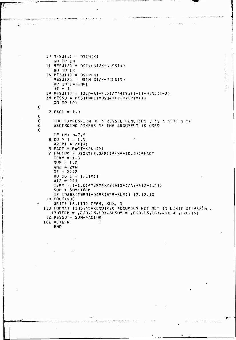
c c c c
11
16
19 18
10
113
12 101
HESJU» = nsiM(x) GH TP 13
GO TP 1", p.rsjm = BESJ(2) = on 1° I=^,NP1 M = I RESJII) = (2./T*AJ-3.0)/X**FSJU-l)~-<ESJ( 1-2) 8ESSJ = P?S.l(^Pl)*OSg>T(2.n/{P[*xj } GO TP 101
)SIN(X) ■isi.\.x)/y-">cris(X)
2 FACT = 1.0
THF FXPPtSsIPN OF A VESSEL FUNCTION' J \S A ASCENDING POWERS OF THE ARGUMENT IS 'JSEO
sr -<r»s
IF |N) 3,7,8 DO 5 I « l,N A2IP1 = ?*!♦! FACT = FACT*X/A2IP1 FACTOR = DS33TI2.0/PI)*<X**(0.5))*FACT TERM = 1.0 SUM = 1.0 AN? ■ 2*N X2 = X**2 DO 10 I = l,LIM IT AI2 = ?*I TERM = (-1.0)*TEPM*X2/(AI2*CAN?+AI2+1.0)) SUM = SIJM+TERM IF (nARS(TERM)-DABS(EPR*SUM)) 12,12,10 CONTINUE WRITE (6,113) TERM, SUM, X FORMAT (lMO,^OHREQUiaEO ACCURACY NOT MET IM LIMIT STI^'S/lH
17HTERM = ,F20.15,10X,6HSUM = ,F20.15,10X.4HX = tF?P.15) RESSJ = SUM*FACTQR RETURN END

^t^-W^SM ««•
C c. c c c c,
EVAIUATIPN O«1 SIMGLF INTEGRAL BY SIMPSOV S «>UI f
C
C
C
C
EXTEFNAl F cn^MrN \', M, \'P, «p, Gnou?, r,cou2, fc.<*^ES, LIMPFS
DIMENSION SINT(lOOr-), INQUQOCJ, INDNU* ( I 000)
PI = 3.141593
READ (*,ll) FRH, FRRSESf LIMITlt LIMIT?» LI'HES, HJW)\T 11 FOPMfiT (2F20.10,M10/I1G)
REAP. (5,1) FR, OHO 1 FORMAT (7F1Q.5)
CCrU? = 1.0/{2.G*FP**2) GDPU2 = GCOU2*mC WRITE (6,?) F>'» GCPU2, GDOU2, 0'',C, ERR
2 FORMAT UfU,2lHFR * U/SQR T( ?*G*C J = ,FI0.5,iOX, 111HG*C/U**2 * ,Flö.5, 10X, llHG*rJ/U**2 = »F13.5,10X, 26HD/C = ♦F10.*>,10X/1HC,6HEKR = »F20.I5)
FACT = B.0*PI* EXP(-2.0*GDOU2) H = 1.0/ SQRT(2.0*GD0U2)
DO 7 I=1,NUMINT i
REAP (5,21) Nf M, NP, MP 21 FORMAT (4110)
INDNUM(I) = 10O0*N*10O*M + 10*\'P+MP IND(I) = N+M+NP+MP
IF ( INPU)/2*2-IND{I)) 25,26,25 26 SINT(I) = 0.0
GO Tn 7
C
C
25 WRJTF (6,61) N» M, IMP, MP 61 FOFMAT (///1H0,4HN = ,I2,iOX,4HM = ,12,10X,5H\P - ,12,
110X,5HKP = ,12) A = 0.0 B = SQPT(10.0)*H SUPS = 0.0 ERUSFD = ERR
DO 14 K=1,LIMIT1
mmmmmL .„:SW.,^:- ^■L--^^--^W-^^-*^^-.f;- -~':*^>-*. uy.imtm .-J'^^k^-Äi;..^.;... -„gfatffä
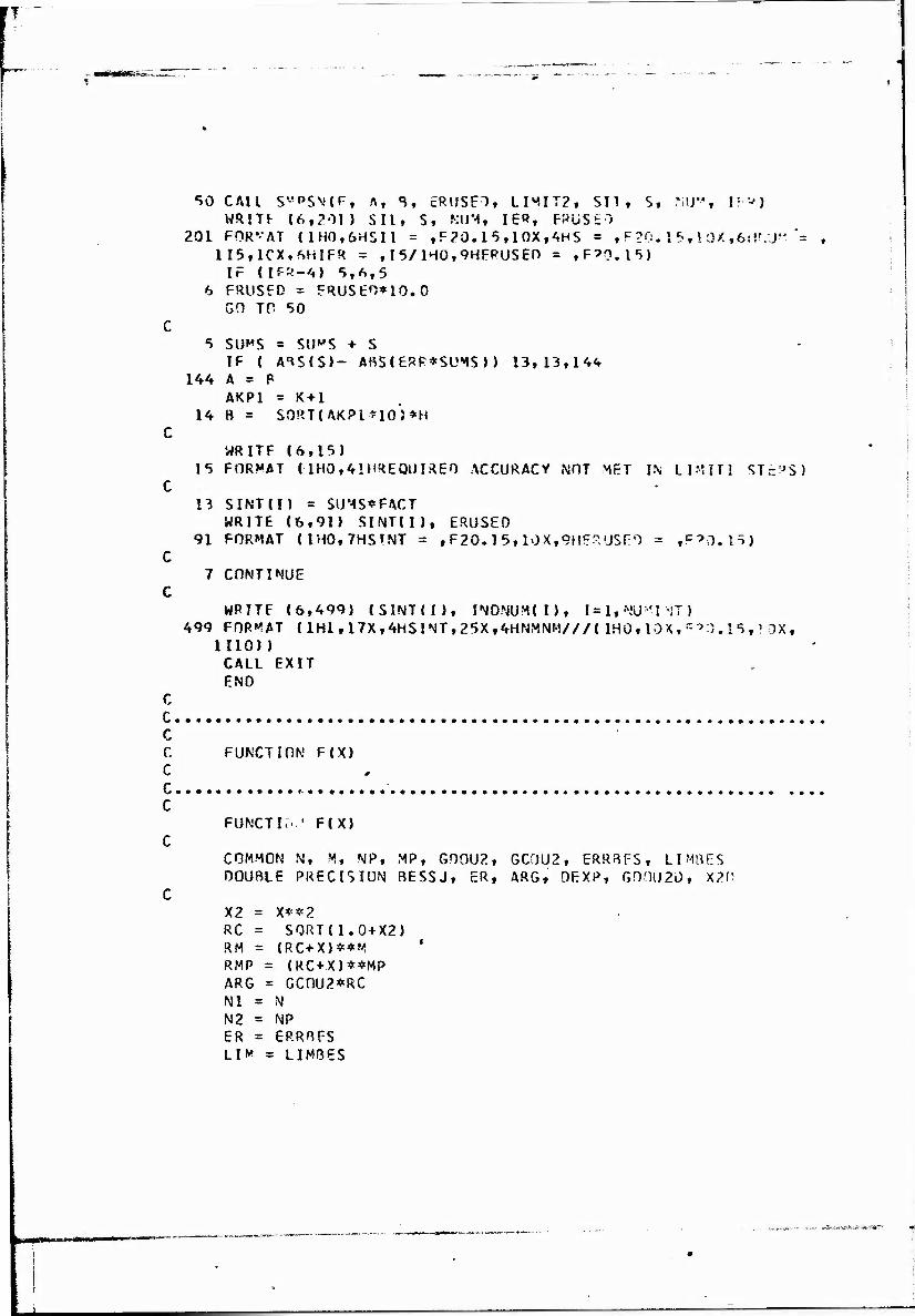
c
c
50 CA1L S«P$\!(F, A, S, ERUSEl, LIMIT2, SI1, S, KU", IF») WRIU (6,201) Silt S, KIJM, IE«, E»üSt"i
201 FOR'-'AT (1H0,6HSI1 = ,F20.I 5,10X,4HS = , F ?0. 1 5 ,! OX ,6:<f.J" '= 1I5,1CX,SHIFR = ,I5/H0,9HFPUSEn = ,F?9.15)
IF Uf«-4) 5,6,5 6 FRUSFD = FRUSE')*10.0
GO TO 50
•» SUMS = SWMS + s IF ( ABS(S)- AS${ERP*SUMS>) 13,13,14*
144 A = P AKP1 = K+l
14 B = SO«T(AKPino')*H
WRITF (6,15) 15 FORM/IT UH0,41HREQUIRE0 ACCURACY NOT MET IN LIMITl ST.-JS)
13 SINTU) = SUMS*FACT WRITE 16,91) SINTU), ERUSEO
91 FORMAT UHQ,7HS!NT = , F2Ö.1 5,10X,9HE3USE0 = ,C?0.15)
7 CONTINUE
WRITE (6,499) (SINTU), INDNUM(I), 1 = 1, NU:'I MT) 499 FORMAT ( 1H1 , 17X ,4HSINT ,25X,4HNMNM/// { IHO, IDX, «='-■). I 5 ,1 OX,
1110) ) CALL EXIT END
C C C C FUNCTION F(X) C C c
c FUNCTir..1 FIX)
COMMON N, M, NP, MP, G00U2, GC0U2, ERRBFS, LIMBES DOUBLE PRECISION BESSJ, ER, ARG, OEXP, G00U2Ü, X2H
X2 = X**2 RC = SQRTU.0+X2) RM = (RC+X)**M ' RMP = (RC+X)**MP ARG = GC0U2*RC Nl = N N2 = NP ER = ERRBFS LI* = LIMBES
„.-... .JVu^ii-An;-... :*;■:-;:
I 1 .'«JJl.U. ... ■!
r""i.J-' M
Goru?n = GDOJ?
X2D = X?
F = C.25*(a^l.u/RV)*{RMP+1.0AMOJ-»1HSSJ(N1 ,4V,,! f ,LI >'.}* 18ESSJ(^.?,4Sr,,ÜKfLr.)/RC*i)EXP(-?.G*GOn!J?r)*X2>)
RETURN TNT
/
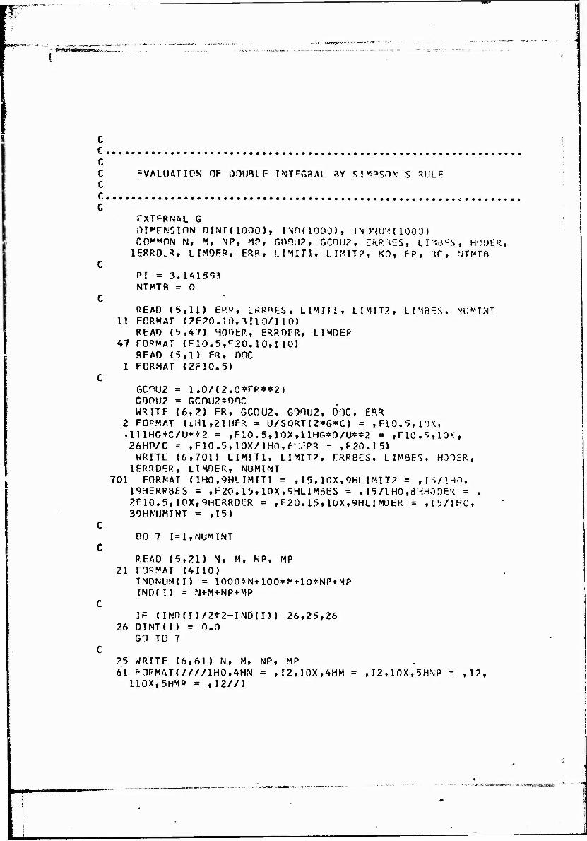
^m^
++**&***»"*»■■
c c c C EVALUATION OF DOUBLF INTEGRAL 3Y SI«DSnK S RULF C C „ c
FXTFRNAL G DIMENSION OINT(IOOO), IMOUOOO), IN0NUMU003) COMMON N, M, NP, HP, G0nt)2, GC0U2, E*»3ES, Ll-IßES, HODER,
1ERRD.*, LIMDFR, ERR, LIMIT!, LIMIT2, KO, FP, <C, NTMT8 C
PI = 3.141593 NTMTB = 0
C READ (5,11) ER», ERR^ES, LIMIT!, LIMIT?, LT1BES, NU^INT
11 FORMAT (ZF29.10,3110/110) READ (5,47) WOOER, ERRDFR, LIMDEP
47 FORMAT (P10.5,F20.10,1 10) READ (5,1) FR, OOC
1 FORMAT (2F10.5) C
GCPU2 = 1.0/f2.0*FR**2) GD0U2 = GC0U2*00C WRITF (6,?) FR, GC0U2, G00U2, DOC, ERR
2 FOPMAT UH1,21HFR = U/SQRT(2*G*C) = ,F10.5,10X, .111HG*C/U**2 ■ ,F10.5,10X,11HG*D/U**2 = ,F10.5,10X, 26H0/C = ,F10.5,l0X/iH0,6!:JPR = ,F20.15)
WRITE (6,701) LIMIT1, LIMIT?, FRRBES, LIMSES, HODER, 1ERRD=R, LIMDER, NUMINT
701 FORMAT (1H0,9HLIMIT1 = ,15,10X,9HLIMIT? = fI5/iH0, 19HERPBES = ,F20.15,10X,9HLIMBES = ,15/1 HO,8 WHO DER = , 2F10.5,10X,9HERR0ER = ,F20.15,10X,9HLIMOER = ,I5/1H0, 39HNUMINT = ,15)
C
C 00 7 I*lvNUMINT
READ (5,21) N, M, NP, MP 21 FOPMAT (4110)
INDNUM(I) = 1000*N+100*M+10*NP+MP IND(I) ■ N+M+NP+MP
IF (IND(I)/2*2-IND(I) ) 26,25,26 26 DINT(I) = 0.0
GO TC 7
25 WRITE (6,61) N, M, NP, MP 61 F0RMAT(////1H0,4HN = ,I2,10X,4HM = ,I2,10X,5HMP = ,12,
110X,5HMP = , 12//)
äiSSföttlMItaKll '.MS. *«tWfi8Äfi£«

A = 0.0 B = 5.0 SUMS =0.0 cRl'SFD = 10.0*ERR
on ;' L=l,LIMITl 50 CAIL SMPSNH3» A,
WRITE (6,201) SI If 201 FORMAT (////lH0,6HS11 =
16HNUM = ,I5,1QX,6HIFR = 2^HA = ,F20.15,10X,4H8 =
IF (IFR-4) 5,6,5 " 6 FRUSED = ERUSED*10.0
IF (FRUSFD.GE.0.1) CALL GO TO 50.
5 SUMS = SUMS + S IF { ARS(S)- ABS(ERR*SUMS) )
144 A * B . 14 B = B + 20.0
B, ERUSED, LIMIT2, SI1, S, NUM, IER) S, NUM, IFR, ERUSED, A, 3
,F20.15,10X,4HS = ,F20.15,10X, ,I5/1H0,9HERUSFD = ,F2O.15,10X, ,F20.15////)
EXIT
13,13,144
BB = B - 20.0 WRITF (6,15) BR
15 FORMAT ( 1H0,41HREQUI*.ED ACCURACY NOT MET IN LIMIT! STEPS, 110X,'.H3 = ,F20.15)
13 OINT(I) = SUMS*GC0U2 WRITE 16,91) DINT(I), ERUSED, 6, SUMS
91 FORMAT (//////1H0,7H0INT = »FJ0.15,10X,9HERUSE0 = » IF2C.15,10X,4HB = ,F20.10/1H0,7HSUMS = ,F20.15)
7 CONTINUE
WRITF (6,499) '(OIMT(I), INDNUM(I), I«lrNUMIMT) 4 99 FORMAT (IH1,17X,4HDINT,2 5X,4HNMNM///(1HO,10X,F20.15,10X,
1110)) WPITF (7,599) (DINT(I), INONUM(I), I = 1,NUMINT)
599 FORMAT (E20.10, 20X, HO)
CALL EXIT END
C C, C c c c, c
FACTION G(U)
FUNCTION G(U) EXTERNAL FM
■x.tsm:

REAL KO, K COMMON N, M, NP, MP f GDOU?, GCOU2, ERRßES, LTM8ES, HOOER, 1ERPDFR, LIMDER, ERR» LIMITl, LIMIT2, KO, EP, U, NTMTfl
C C THE DERIVATIVE OF THE FUNCTION AT KO = l.O+U**2 IS C EVALUATED BY DIFFERENTIATING AN INTERPOLATION POLYNOMIAL C IF THE FOURTH DEGREE C
KO = 1.0+U**2 RC = SQRT(KO) ERDEP = FRRDER
3 H * HODER PFP = 0.0 DO 10 J-l,LIMDER H = H/2.0 FP = (F(K0-2.0*H)-8.0*F{K0-H)+8.0*F{K0+H>-F{K0+2.0*H)) 1/(12.0*H) IF ( A^S(FP-PFP)- ABSlFP*ERDER)) 4,4,10
10 PFP = FP C
WRITE (6,60) U, FP, H 60 FORMAT (////1H0,41HREQUIRED ACCURACY NDT MET IN LIMDER STEPS,
15X,4HU = ,F20.15,5X,5HFP = ,F20 . 15 , 5X ,4HH ~ ,«=20.15) IF ( ARS(FP).LE.l.0E-14) GO TO 4 ERDFR = ERDER*10.0 IF (ERDER.GT.0.1) CALL EXIT GO TO 3
C 4 SUMS =0.0
ERUSED = ERR A = 0.0 B = 0.0 U2 = U**? DO 9C I = 1,LIMITl A = ß B = B + 2.5/GDOU2 IF (P-.GF.U2) B = U2
91 CALL SMPSN !FM, A, B, FRUSED, LIMIT2, SI 1, S, NUM, IFR) IF (IER-4) 77,88,77
88 FRUSED = ERUSFD*10.0 IF (ERUSED.GE.0.1) CALL EXIT GO TO 91
77 SUMS = SUMS + S IF (B-U2) 96,92,92
96 IF ( A1S(S)- ARS(ERR*SUMS)) 97,97,90 90 CONTINUE
C WRITE (6,93) U
93 FORMAT (IH0,32HKMAX GREATER THAN 2*L I MIT 1/O0U2 ,1 OX ,

...... ,.....^ . .-=;--,;--y-v ^;-:N«-;.r^!?- ■*StfStt*W ^ ;V- V.^^-
1
14HU = ,F20.i5) CALL EXIT
97 A = U2 R = 2.0 + U2 FRUSED = ERR [MAX = 5 CALL SMPSN (FM, AT B, ERUSED, IMAX, SI1, PVAL, MUM, IER) IF ( ABS(PVAL)- ABS(EPR*SUMS)) 13,92.92
92 A = U2 B = 2.0 + U? ERUSED = ERR
94 CALL SMPSN (FM, A, B, ERUSED, LIMIT?, SI1, °VAL, NUM, IER) % IF (IFR-4) 55,66,55
66 IF ( ABS(PVAL)- ABS(ERR*SUMS)) 55,55,606 606 ERUSED = ERUSED*10.0
IF (ERUSED.GE.0.1) CALLFXIT GO TO 94
55 SUMS = SUMS + PVAL
A = B B = B + 2.0/GDOU2 FRUSED = ERR DO 14 L=1,LIMIT1
50 CALL SMPSN (FM, A, B, ERUSED, LIMIT2, SI1, S, MUM, IER) IF (IER-4) 5,6,5
6 IF ( ABS(S)- ABS(ERR*SUMS)) 5,5,6666 6666 ERUSED = ERUSED*10.0
IF (FRUSED.GE.0.1) CALL EXIT GO TO 5 0
5 SUMS = SUMS + S IF { ABS(S)- ABS(ERR*SUMS)) 13,13,144
144 A * R 14 B = B + 2.0/GD0U2
WRITE (6,15) U, 3 15 FORMAT (1H0,41HREQUIR£D ACCURACY NOT MET TM LIMIT1 STEPS,
110X,4HU = ,F20.15,10X,4hB ■ ,F20.15) NITNTD = NTMTB + 1 IF (NTMTB.GT.50) CALL EXIT
13 RM = (1.0+U/RC)**M RMP = ( 1.0+U/RC)**MP G = (RM+1.0/(RM*(KO**M)))*(RMP+1.0/(RMP*C<0**Ma)J )/ .
l(RC**(N+NP+2-M-MP)1«SUMS WRITE (6,301) SUMS, U, G, 0
301 FORMAT (1H0,7HSUMS = , F20.1 5 ,1 OX ,4HU = ,F20.15,10X, 14HG = ,F20.15,10X,7.-IKMAX = ,F20.10)
* V.k.-^&^-r^i1^: 'W&J%,.-

c c. c c c
KFToS-N
FUNCTION FK{*)
C C. r
c c c« c
FACTION F?U) SFAL KO, COKMt'N
IF^OEK, COKHCN N, y, NP, y.p, GO
Ll-JER, e GCÜU2, FRRBES, LI'Ats», HODrR,
RP, LIMITlt L-niT2t XO, FP, *C Ol»?i
IF (K-KO) 3,2,3 3 FM = F(K)/IK-KO)
RETURN 2 FM = FP
RETURN END
FUNCTION F<K)
FUNCTION F(K) REAL KO, K COVMCN N, V, NP, ?',P, GOCU2, GCOU2 , FRR3ES, LIEBES, 1ERROER, LIMOER, E.RR , LIMITl, LIMIT2, KO, FP, RC DOUBLE PRECISION BESSJM, ER, ARG, DEXP, GDOU2D, KO
HOOER,
ARG * Nl = .\? = EH = Liy = GOCU? KO = F = { 1BES5J KETUR END
»COU2*K/RC N NP ER L
D K K + M( N
KBES IWRES = GOCU2
KO)*OEXP(-2.0*KD*GDOU2D)*((GCOU2*K)♦+ ( M+NP)) N].,ARG,ER,LIP)*BESSJM(N2,ARG,ER,LIM)

'--~- ^M£& '■&•■- *»^***f^^ffit-Ä» J MB«HMMRNAMBm
c c, c c c c c c c, c
c c c c c
FUNCTION 8FSSJM
RFSSFL FUNCTION J OF ORDER N+i/2 DIVIDED 1Y TH: ARCUMFNT RAISED TO THE N + l/2 POWER
DOUBLE PRECISION FUNCTION RFSSJM<N,X,PRR,LI MIT) DOUBLE PRECISION X, ERR,
1DCOS, OSORT, DABS, BCSJ, DIMENSION BESJI100) PI = 3.1415926535998 IF {X-5.0J 2,2,3
3 NP1 = N+l
THE RECURRENCE RELATION J(N+1,X)+J(N-1,X> »
IS USFO
PI, FACTOR, TERM, SUV, x?t DSIN, FACT
(2*N/X)*J(N,X)
13
11
16
19 IB
IF (N-l) 13,11,16 RESJ(1) = DSIN(X) GO TO 18 BESJ(2) = DSINIX)/X-DCOS(X) GO TO 18 3FSJ(1) = BFSJ(2) = DO l"i 1 = 3, NP1 AI = I BESJ(I) = (2.0*AI-3.0)/X*3FSJ(1-1)-BFSJ(1-2) BESSJM = BESJ(NP1)*0SQRT(2.0/PI)/(X**(N+1)) GO TO 101
f)SIN(X) DSINIX)/X-DCOS(X)
C c c c
2 FACT = 1.0
THF EXPKFSSION OF A BESSEL FUNCTION J AS A SERIES OF ASCENDING POWERS OF THE ARGUMENT IS USE.D
IF (Nl 8,7,8 « 8 00 5 I = 1,N
A2IP1 = 2*1+1 5 FACT = FACT/A2IPI 7 FACTOR = 0SQRT(2.0/PI)*FACT
TERM = 1.0 SUM = 1.0 AN2 = 2*N
. ;..-JövW«M<-.s ■ i-ilivK^ww^-^imtfjrtäXMiWti,:^- ta&tftt

ffMPlÖB^HSP'Wfc^B'S^'Jp-"'"3 LÄ* Wp*^S?SBK!St^Ö!WjGÜ?i?43^'BSI'^Ö
x? = x*+? DO 10 1=1,LIMIT AI? = 2*1 TFRM = (-l.0J*TERM*X2/(AI2*(AN2*AI2*l.0H SUM = SUM+TERM IF ?OABSlTERM)-DABS!FRR*SUM»> 12*12,10
10 CONTINUE WRITE 16,1131 TERM, SUM, X
113 FORMAT f1HO,40HREQUIRED ACCURACY NOT MET IN LIMIT STEPS/IH , 17HTFPM * ,F20.15,10X,6HSUM = ,F20.15,10X,4HX = ,F20.15)
12 BESSJM » SUM*FACTOR 101 RETURN
END
_

»i«S>»fvs»-3S,5SB5S9e*e aamemm m gag» *mu
r. c. c c c c c c,
SOLUTION OF THE SYSTEM OF EQUATIONS
(I-B)A = R
C
c
c
c
c
c
c
DIMENSION AINT(20,2O), 0120,20). INO(?0,20), INDNUM(?Q,20) DIMENSION N(20,20)« M(20,20), NP(20,20), MP(20,20> DIMENSION 8C20*20), BB(20,20), BCOLC40Q), R(23)
REAO (5,1 I EPS 1 FORMAT (F20.10)
REAO (5,2) NUMAOC, NUMSYS, MNUMEQ 2 FORMAT (3110)
READ (5,61) (UINT(I,J),N(I,J),N(I,J),NP(I,J),MP(I,J), U=I, I), 1 = 1,MNUMEQ)
61 FOP MAT (E20.10,26X,4U)
rfRITF (6,991) ((AINTfI,J),N(I,J),M(I,J),NP( I,J),MP(I,J), U=lt I). 1=1. MNUMEQ)
991 FORMAT (lHl/(IH0,F20.10,10X.4II))
MNFQM1 = MNUMEQ-1 00 10 I-1.MNEQM1
IP1 = 1+1
00 10 J=IPI,MNUMEQ
AINT(I.J) = AINT(J,I) NU,J) = NP(J,I) M(I,J) = MP(J,I) NP(I,J) = N(J,I) MP(I,J) = M(J,I)
10 CONTINUE
DO 20 1 = 1,MNUMEQ
00 20 J=l,MNUMEQ
INO(I,J) = N(I,J)+M(I,J)+NP(I,J)+MP(ltJ) INDNUM(I,J) » lOOO*Nil,J)*100*M(I,J)+10*NPi I,J)+MP(I,J)

c
c
c
c
c
IF l(ND(Iv J)/?*2-lND( I,J>) 25,26,25
26 OU,J) * AINT(I,J)*(-l)**(IMQ(I,.)l/?+NP( I,j)) GO TO 20
25 0(I,J) = AINTCI, J)*(-l)**UINO(I, J )♦ 1)/2*NJ»( I , J) )
20 CONTINUE
WRITE (6*662) 662 FORMAT! IM,11HMATRIX AfNT////)
WRITE (6*62) KAINTIIv J1,J=1,MNUMEQ),1=1,MNUMEQ) 62 FORMAT (1H0,9E14.6/1H0,9E14.6/1H0,98X,2FtA.6)
WRITE (6,31) 31 FORMAT (1H1,8HMATRIX D////)
WRITF (6,13) ((D(l,J),J=l,MNUMEQ),1 = 1,MNUMEQ) 13 FOPMAT (IH0,9E14.6MH0,9E14.6/IH0,98X,2F14.6)
00 501 K=1,NUMA0C
REAO (5,213) A0CM1 213 FORMAT (F20.I0)
AOC = AOCMH-l.O WRITE (6,41) AOC "
41 FORMAT (1HI,6HA/C = ,F10.8)
CALL MATRIXI9,Bö.QDOTl,MNUMEQ,A0CM1)
WRITE (6,73) ((BB(I,J),J=l,MNUMEQ),1=1,MNUMEQ) 73 FORMAT 1////IH0,8HMATRIX 3//7/(1H0,9E14.6)/1H0,9E14.6/
11H0,98X,2E14.6) C
00 515 1=1,MNUMEQ 00 515 J=i,MNUMEQ
515 B(I,J) = -l.O*BB(I,J) C
DO 51 1 = 1,MNUMEQ 51 Bf1*11 = i.O-BB(I,I)
C WRITE (6,74) HB(I,J),J=l,MNUMEQ), 1 = 1,MNUMEQ)
74 FORMAT (////IHO,12HMATRIX (I-B)////(1H0,9E14.6)/1H0, 19E14.6/1H0,2E14.6)
C WRITE (6,14) QD0T1
14 FOPMAT (////IH0,8HQ00TI = ,E14.6) RID = -1.0/QD0T1 WRITE (6,99) R(l)
99 FORMAT (IH1,7HR(1) = ,E14.6)
C
C
: vxM&zit. ■ ■-■ ..iififtj •-^jnfriHMjfttt'ir'* I '**

—.-Jt iJr *j&j3%
.,- mv~tsmmmamm&m?>B*mMmt WBm&Mi<*ss&wem»smm*!meaim*<x i i m ■ IL ■ MMM—MB—a——■———^J*^
NUMEO =0 00 501 KK=1,NUMSYS
C NUMEO = NUMEO ♦ (KK+1)
C 00 2272 1=1,NUMEO
2222 *(I) = 0.0 R(l) = -1.0/3D0T1
C 00 97 J=l,NUMEO 00 97 1=1,NUMEO ' L = CJ-l)*NUMEO*I
97 RCOLfL) = BU,J) C
CALL GELGIR,BCOL.NUMEO,1,EPS,IER) C
WRITE (6,16) IER 16 FORMAT (//////1H0,6HIER = ,15)
WRITF (6,17) (R(I),I=1,NUMEQ) 17 FORMAT (//IH3,6HA10 = ,E14.6,5X,6HAl1 = ,E14.6/IHO,6HA20 = ,
IE14.6,5X,6HA21 = ,E14.6,5X,6HA22 = ,E14.6/1H0.6HA30 = »F14.6, 1 5X.6HA31 = »E14.6, 5X.6HA32 = «E14.6, 5X,6HA33 = ,E14.6/1H0, 16HA40 = ,E14.6, 5X,6HA41 = ,F14.6, 5X,6HA42 = »E14.6, 5X, 16HA43 = ,E14.6, 5X.6HA44 = ,E14.6/1H0,6HA50 = ,E14.6, 5X, 16H&51 = ,E14.6, 5X.6HA52 = ,E14.6, 5X,6HA53 = ,E14.6, 5X, 16HA54 = ,E14.6/1H0,100X,6HA55 = ,E14.6i
C WRITE (7,717) (R(I), I, KK, AOC, I=1,NUMEQ)
717 FORMAT (E20.10,I10,20X,I10,10X,F10.6) C
501 CONTINUE C
CALL EXIT END
C C c C SUBROUTINE MATRIX(0,B,0D0T1,NUMEO,A0CM1) C C PURPOSE C C OBTAIN THE AUGMENTED MATRIX OF THE SYSTEM OF EQUATIONS C C (I-8)A = C C C «, C
SUBROUTINE MATRIX(0,B,QD0T1,NUMEO,A0CM1)
- ' —■ ■'- --Tfi'^M

1
c
c
c
c
jw%POfSL-cs^sÄ«t ,- - -■■i^T^~--iiN4-a&r5*5**?**St^*^?^i?l^'-'1
DIMENSION 0(20,20), B(?0,20) OIMFNSION POL(IO), OPOLIIO), QOLdOJ» DQOL(IO), PUO.iO),
IDP(IOflO), QUO,101, DQ(10,10), DPDQ(10,10), OPLOOL(IO) DOUBLE PRECISION 00, POL, DPOL, OOL, DQOl, P, OP, 0, 00, XM1
1DP0Q, DPLOOL
XM1 = A0CM1 CALL LEGF{00,POL,DPOL•OOL,?GOL,P,DP,Q,DQ,XM1)
NDEG = 5
WRITE 16,32) 32 FORMAT I////IHO,ilHFUNCTIONS PI
WRITE (6,11) (POL(I),CPU,J),J=l,I),1 = 1,NDEG)
WRITE (6,33) 33 FORMAT (/MHO, IlHFUNCTIONS Q)
WRITE (6,11) (QOLCI),(Q(I,J)tJ=l,I),I=l,NDEG)
WRITE (6,34) 34 FORMAT (//IH0.30HDERIVATIVES OF THE FUNCTIONS P)
WRITE (6,11) (DPOLU),(DP(I,J),J=l,I),1=1,NOEG)
WRITE (6,35) 35 FORMAT (//1H0,30HDERIVATIVES OF THE FUNCTIONS 0)
WRITE (6,11) (DQOL(l),(DQ(I,J),J=l,I),I=l,NDEG)
11 FORMAT (lH0,2F25.15/lH0,3F25.l5/lH0,4F25.15/(1H0,5F25.15))
DO 87 1*1,NDEG DPLDOL(I) = DPOL (I)/DQOL U) 00 87 J=1,I
87 DPDQU,J) = OP(I,J)/DQ( I,J)
WRITE (6,3 ) 36 FORMAT (//IH0,20HP00T OIVIDFO BY ODOT)
WRITE (6,11) (OPLD0L(I),(0P00(I,J),J=l,I),1=i,NDEG)
DO 50 J=1,NUMEQ 8(1,J) = DPLDQL(l)*D(l,J)*3.0/4.0 B(2,J) « DPDQ(l,l)*D(2,J)*3.0/2.0 B(3,J) = DPLD0L(2)*D(3,J)*5.0/4.0 B(A,J) = DP00(2,1)*D(4,J)*5.0/2.0 B(5,J) = DPDQ(2,2)*D(5,J)*5.0/2.0 B(6,J) = DPL0QL(3)*D(6,J)*7.0/4.0 B(7,J) = DPD0(3,i)*D(7,J)*7e0/2.0 B(8,J) * DPDQ(3,2)*0(8,J)*7.0/2.0 8(9,J) - DPDQ(3,3»*D(9,J)*7.0/2.0
1

I ■'■-;'-%-»"■;--"* '^™s*'' »KSES5 _-■
B(10tJ) P(lltJ) R(12,J) S(13«J) B(!4,JJ 8I15.JI B(16,J) B(17,J) 8(18,J» B(19,J) B(20,J>
DPL0QLC4) 0P0Q(4,l) DPDQ(4,2) DP0Q{4,3) DPDQ(4,4) DPLD0L15: DP00(5,1» 0PDQ<5,2) DPD0(5,3) 0PDQt5,4) 0P00(5,5)
*D(10,J *0(ll,J *D(12,J ♦0(13,J *0{14,J ♦0(15,J *D(16,J *0(17,J ♦9(18,J *0(19,J *0C20,J
C
c
c
c c. c c c c c c c c c, c
)*9.0/4.0 )*9. 0/2.0 >*9.0/2.0 )*<».0/2.0 )*9. 0/2.0 1*11.0/4.0 )*11.0/2.0 i*ll.0/2.0 I' 11.0/2.0 )*11.0/2.0 1*11.0/2.0
50 CONTINUE
Q00T1 = OQOLtl)
RETURN ENO
SUBROUTINE LEGFCQOtPO*,DP0L,0OL,0QOL,P, DP,Q,DQ,XM1)
PURPOSE.
EVALUATE THE LEGENORE FUNCTIONS AND THEIR FIRST DERIVATIVES FOR VALUES OF THE ARGUMENT GREATER THAN 1 AND DEGREES UP TO 5
SUBROUTINE LEGF(00,POL,DPOL,QOL,DQOL,P, DP,Q,DQ,XM1)
DIMENSION POL(IO), DPOL(IO), QOt(lO), DOOL(IO), P(10,10), IDP(10,10), 0(10,10), DQ(10,10) D0U8LE PRECISI1N QO, POL, CPOL, OOL, DQOL, P, DP, Q, DO,
IX, XM1, X2MI, X2M12, X2M13, RC, RC3, RC5, RC7, DLOG, DSQRT
X = l.O+XMl X2M1 = XM1*(2.Q+XM1) X2M12 = X2M1*X2M1 X2M13 = X2M12*X2M1 RC * 0SQRT(X2M1» RC3 = X2M1*RC RC5 = X2M12*RC RC7 = X2M13*RC
PQL(1> = POL 12) = P0H3I =
1.5*X2M1+1«0 2.5*X*X2M1*X
.*v.v.:..-- ..,-.v-.'.,..^, ( i f$&$3m ■asm

^T
KM»g(KiS*fc- :«."-".:Wf»i»
P0K4) = 4.375*X2M12+5.0*X?MH-1.0 POLIS» = X*17.875*X2Mi2+7.0*X2Ml+1.0>
DPCL(l) = 1.0 DPOL(2) = 3.0*X DPOL(3) = 7.5*X2Ml+6.0 DP()L(4) = X*(17.5*X2M1+10.0) DPOL15) = 315.0/8.0*X2M12*52.5*X2M1*15.0
C
C
Pfitl) = RC P(?,l) = 3.0*X*RC P(2t2) = 3.0*X2M1 P!3,l) = 7.5*RC3+6,0*RC P(3,2) = 15.0*X*X2M1 P<3,3) = 15.0*RC3
P(4,l) = X*(17.5*RC3+lO.0*RC) PIA,2) = 7.5*(7.0*X2M12+6.0*X2M1) P(4,3> = 105.0*X*RC3 Pt4,4) = 105.0*X2M12
P«5tl) = 315.0/8.0*RC5+52.5*RC3+15.0*RC P(5,2) = 52.5*X*(3.0*X2M12+2.0*X2M1) P(5,3> = 52.5*<9.0*RC5+8.0*RC3) PC5.A) = 945.0*X*X2M12 P(5,5) = 945.0*RC5
DP(l,l> = X/RC DP(2»1) = 6.0*RC+3.0/RC DP(2,2) = 6.0*X DP(3,1) = 1.5*X*(15.0*RC+4.0/RC) DP<3,2) = 45.0*X2Ml+30.0 DP(3,3) = 45.0*X*RC
DP(4,1) = 70.0*RC3+72.5*RC+10.0/RC DP<4,2> = 30.0*X*(7.0*X2MH-3.0) DP<4,3) = 105.0*(4.0*RC3+3.0*RC) DP(4t4) = 420.0*X*X2M1
DP(5,1) = 15.0/8.0*X*(105.0*RC3+84.0*RC+8.0/RC) OP(5T2) = 52.5*(15.0*X2Ml2+l«.0*X2Ml+4.0) 0P(5,3) = 52.5*X*t45.0*RC3+24.0*RC> DP(5,4) = 945.0*<5.0*X2M12+4.0*X2Ml) DP(5,5) = 4725.0*X«RC3
00 = 0.5*(DLOG(2.0+XM1)-OLOG(XM1))
QOL(l) = X*Q0-1.0 Q0U2) = (U5*X2Ml+1.0)*Q0-l.5*X
~J

Q0U3) = X*(?.5*X2Ml+l.Ü)*Q0-?.5*X2Ml~ll.000/6.OOC m(4) = (4.375*X2M1?*5.0*X2M1-H.0)*00-X*(4.375*X2MU
l.!5.000/12.000) CPLI5) * X*(7.875*X2Ml?+7.0*X?Ml + 1.0)*Q0-7.875*X2r*12-
19.625*X?M1-137.000/60.000
D'jnLll) = Q0-X/X2M1 DQr.LC?) = 3.0*X*QO-3.0-l.0/X2Kl 0QPL(3) = (7.5*X2M1+6.0)*Q0-7.5*X-X/X2M1 O0OU4) = 2.5*X*(7.0*X2M1+4.0)*00-17.5*X2M1-95.000/6.000-
11.0/X2MI 0001.(5) = 15.0/8.0*(21.0*X2M12+28.0*X2Ml+3.01*00-105.0/8.0*
lX*i3.0*X2Ml+2.0)-X/X?Ml
0(1,1) = QO*RC-X/RC 0(2,1) = 3.0*X*RC*00-3.0*RC-1.0/RC 0(2,2) = 3.0* X2M1*Q0-(3.0*X**3-5.0*X)/X2M1 0(3,1) = (7.5*X2M1+6.0)*RC*00-7.5*X*RC-X/RC 0(3,2) = 15.0*X*Q0*X2Ml-15.0*X2Ml-5.0+2.0/X2Mi 0(3,3) = 15.0*RC3*QO-X*(15.0*RC-10.0/RC+8.0/RC3)
0(4,1) = X*(l7.5*X2Ml+10.0)*RC*QO-17.5*RC3-95.000/6.000* 1RC-1.0/RC Q(4,2) = (52.5*X?M12+45.0*X2M1)*Q0-52.5*X*X2M1-10.0*X+
12.0*X/X2M1 0(4,3) * l05.0*X*RC3*Q0-L05.0*RC3-35.0*RC + 14.0/RO8.0/RC3 0(4,4) = 105.0*X2M12*Q0-X*(105.0*X2Ml-70.0+56.0/X2M1-48.0/
IX2M12)
0(5,1) = 15.0/8.0*(2l.O*X2M12+28.0*X2Ml+8.0)*RC*00-X*( 1315.0/R.0*RC3+26.25*RC + 1.0/RC) .- Q(5,2J » 52.5*X*(3.0*X2M12+2.0*X2M1)*Q0-157.5*(X2M12+X2MD- 114.0+2.0/X2MI Q(5,3) = 52.5*(9.0*X2MI+8.0)*RC3*QO-472.5*X*RC3-105.0*X* 1RC+2 8.0*X/RC-8.0*X/RC3 0(5,4) = 945.0*X*X2M12*QO-945.0*X2M12-315.0*X2MI+1?6.0- 172.0/X2M1+48.0/X2M12 0(5,5) = 945.0*RC5*00-X*(945.0*RC3-630.0*R:+504.0/RC- 1432.0/RC3+384.0/RC5)
0Q(1,1) = X/RC*Q0-l.0/RC+1.0/RC3 D0(2,l) = (6.0*RC+3.0/RC)*Q0-6.0*X/ROX/RC3 00(2,2) = 6.0*X*QO-6.0--2.0/X2M1-4.0/X2M12 DQ(3,1) = X*(22.5*RC+6.0/RC)*Q0-22.5*RC-U.5/RC + l.0/RC3 00(3,2) = (45.0*X2Ml+30.O)*Q0-X*(45.0+4.0/X2M12) 0Q(3,3) = 45.0*X*RC*Q0-45.0*RC-15.0/RO6.0/RC3+24c0/RC5 •
D0(4,l) = (70.0*RC3 + 72.5*RO10.0/RC, -Q0-X*(70.0*RC+ 1155.0D0/6.0D0/RC-1.0/RC3)
- .•,*m«!s«,«ff***'jiaja&v..»5»aäi«>j^^

1'
00(4,2) = 30.0*X*(7.0*X2M1 + 3.0)*QO-210.0*X2M1-1<SO.O-2.C/ IX2M1-4.0/X2M12 00(4,3) = 105-.0*(4.0*X2Ml+3.0)*RC*Q0-X*(420.0*t*O35.0/RO 114.0/RC3-24.0/RC5) 00(4,4) = 420.U*X*X2Ml*Q0-140.0-420.0*X2Ml + 5ft.0/X2M1-
132.0/X2M12-192.0/X2M13
D0(5,l) = 15.0*X*(105.0/8.0*X2Ml+10.5+i.0/X2Mi)*RC*Q0- 11575.0/8.0*RC3-1785.0/B.O+RC-165.0/4.0/RC+1.0/RC3 DQ(5,2J = 52.5*(15.O*X2M12*ia.0*X2Ml+4.0)*00-78 7.c;*X*X2Ml-
1420.0*X-4.0*X/X2M12 00(5,3) = 157.5*X*(l5.0*X2Ml+8.0)*RC*Q0-236?.5*RC3-2047.5*
IRC-105.0/RO12.0/RC3+24.0/RC5 " 0Q(5,4) = 945.0*(5.0*X2M12+4.0*X2*U)*QO-4725.0*X*X2M1-
1630.0*X-*144.0*X/X2M12-192.0*X/X2M13 DQ(5t5) = 4725.0*X*RC3*QO-*725.0*RC3-1575.0*RC+630.0/RC-
1360.0/RC3+240.0/RC5+1920.0/RC7
RETURN END
■.!-.■ --*.--."■-.««Bii«s"!';s»!Siä.* sssassaaa
C c c c c c. c c c c
c
c
DENSITY OF SOURCE DISTRIBUTION
f
PLEASE DRAW WITH BLACK INK
DIMENSION POLHIO), Pl(10,10), POL(lO), P(lO,lö) DIMENSION A(20,6), N(20), M(20) DIMENSION FACTOR(20,1815, SIGMAUU81), THFTA(181),
lTHPDEGURl) DIMENSION DATA(4üO), X(IOOO), YUOOO) DUUBLE PRECISION XM1, POL1, Pl? POL, * CALL TRAPS<-1,-1)
31
CALL PLOTS(DATA,400,7HDENSITY)
READ (5,1) AOCM1 FORMAT (F20.10) AOC = AOCM1+1.0 AOC2M1 = AOCM1*(AOCM1+2.0) FAC « SQRT(AUC2Ml)*l?.566372 WRITE (6,31) AOC FORMAT UHi,6HA/C = ,F10.8)
C
C
READ (5,2) MNUMEQ, NUMSYS, NTHETA, NUMFI 2 FORMAT (4110)
WRITE (6,32) MNUMEQ, NUMSYS, NTHETA, NUMFI 32 FORMAT (1H0,9HMNUMEQ = ,J3,10X,9HNUMSYS = ,I3,10X,
19HNTHETA = ,I 3,10X,8HNUMFI = ,13)
1 = 0 NMAX = NUMSYS-1
DO 10 L=1,NMAX LP1 = L+l DO 10 LL=1,LP1 I ~ 1 + 1 N(I) = L
10 M(I) = LL-1
33 C *
WRITE (6,33) (N(I),M(I),1=1,MNUMEO) FORMAT (////1H0,4H N M//(1H ,212))
XM1 = A0CM1 CALL PNMXG11P0L,P,XM1)
f««|

c
c
DO 17 K=1,NTHETA
NTHEM1 = NTHETA-l ANTHKl = NTHEM1 KM1 = K-l AKM1 = KM1 THfcTA(K) = 3.141593/ANTHMl*AKMl THFDtGlK) = 180/NTHEMI*KM1 X(K> = THEOEG(K) FACT = SQRT((*OC* COS(THETA(K)))*(AOCMl+l.0-
l CCS(THETA(K))))*FAC
XM1 = COS(TH£TA(K))-1.0 CALL PNMXLI(P0LI,P1,XM1)
DO 17 J=1,MNUMEQ
I MJ = K(J) | NJ = N(J)
C
C
C
C
IF (MJ.EQ.O) FACTOR(JtK) = -1.0*POL1(NJ)/POL(NJ)/FACT SSIGN = <-l)**(MJ+l) IF IMJ.NE.O) FACTOR(J,K) = SSIGN*P1(NJ,MJ)/P(NJ,*J)/FACT
17 CONTINUE
NUMEC = 0
00 277 K=l,NUMSYS
NUMEO ■ NUMEQ+K READ 15,7) (A(I,K),I=1,NUMEQ)
7 FORMAT (E2Q.10) WRITE 16,77) NUMEQ
77 FORMAT (lHi»40HCOEFFICIENTS ANM, NUMBER OF EQUATIONS = ,1?) WRITE (6,777) (Nil), M(I),AU,K) ,1 = 1, NUMEQ)
777 FORMAT (///{1H0,1HA,2I2,4H = ,E20.10)) C
IF (K.EQ.l) NUMEQ = 0 277 CONTINUE
C Nl = NTHETA N2 = Nl+1 N3 = Nl+2 X(N2) = 0.0 X(N3) * 9.0 Y(N2) = -0.10 Y(N3) = 0.02 WRITE (6,500) X(N2), X(N3), Y(N2), Y(N3), N2, N3
.^..»^^J»*^-'J^^>-'■^^fc•'*•;*»wi\Sl^■■ll^>w.-.^^a33ta-*s'■1,■"■■ ■■%■ -«*

-«.-U1
^'p*^%mwsmmmmmm*&mt*gmmimm»v&tti'***
500 FORMAT {//////1H0,4F1C.5,2I10)
DO 27 KFI=l,NUMFI
NUFU'l = NUMFI-1 ANFIM = NUFIM1 Kf-IMl = KFI-l AKMM1 = KFIM1 FlOnC = 180/NUFIMI*KFIM1 FI = 3.141593*AKFIH1/ANFIM1 NUMEQ = 0
C
C
c
21
211
CAIL PLLT(6.0,-10.5,-3) CALL PLOT (0.0,0.75,-3)
CALL AXIS(0.0,0.0,11HANGLE THETA,-11, 20. 0, G. C, X( f\2) ,X{ N3) ,20.0> CALL AXIS(0.0,0.0,7HÜENSITY,7,10.0,90.0,Y(N2),Y(N3),20.0) CALL SYMBOL(2.0,8.5,0.14,5HFI = ,0.0,5) CALL NUMBER(3.0,8.5,0.14,FIDEG,0.0,1)
DO 26 KK=i,NUMSYS
NUMEO = NUMEQ+KK
DO 211 K=1,NTHETA SIGMAU(K) = 0.0 DO 21 J=1,NUMEQ AMJ = M(J)
SIGMAU(K) = SIGMAU(K)+A(J,KK)*FACTOR(J,K)* C0S( AMJ*FI) Y(K) = SIGMAU(K) CONTINUE
WRITE (6,22) NUML'Q,FIDEG 22 FORMAT (1H1,22HNUMBER OF EQUATIONS = ,I2,10X,5HF1 = ,F10.5)
WRITE (6,222)'(SIGMAU(K),THETA(K),K=1,NTHETA) 222 FORMAT (IHO,10X,7HSIGMA/U,23X,5HTHETA//(1H0,F20.10,10X,
1F20.10))
C
C
CALL LINE
26 IF (KK.EQ.l) CONTINUE
(X,Y,N1,1,0,0)
NUMEQ = 0
CALL PL0T(20.0,0.0/-3)
27 CONTINUE CALL EXIT END
>~<'<»M«£«^#aMMitt*K'3W)MäilUflH

■ „ - **fr 9H53tm?mk -*. >^www
fjmm*mwm+mtm*w\m*m
C EVALUATION OF THF WAVE RCSISTANCF C C... , c
DIMENSION AINT(20,20>, r<20,20), IND(20,20), I "n\MJM( 20,20} DIMENSION N(20,20), N!(20,20), NP<20,?0), MP{20,?0) DIMENSION NNI20), MMI20), A<20,6), AM20,20) OIMFNSION S(2O,20), SUMC20)
C READ (5,201) NUMAOC, NUMSYS, ?.NU*EQ
201 FORMAT I 3110» C
READ (5,61) {{AINT(l,J),NU,J),MIl,J),NPt I,J),MP(I,J), U«lf l)tI*l»MNUMEQ)
41 FORMAT IE20.10,26X,4U) C
WRITE 16,091) UAINTU,J),N(I,J),M(I,J),NP<I,J),VP(I , J) , U=ltI),I = ltMNUMEC)
<J91 FORMAT (1HI/I1H0,F20.10,10X,4U)) C
MNEQMl = MNUMEO-l DO 10 I=1,MNEQM1
C
C
C
C
c
c
c
c
c
IPI = 1+1 J
00 10 J*IPl»MNUMEQ
AIKTII ,J) = AINT(J,I) NU,J) = NP(J,I) M(I,J) = MPU,I ) NP(I,J) = N(J,I) MP(I,J) = M(J,I)
10 CONTINUE
DO 20 I = 1,MNUMEQ
00 20 J=l,MNUMEQ
INDd.J) = NUtJ)*MU,J)+NP(I,J)+MPU,J) INDNUM(ItJ) = 1000*NlI,J)+100*M(I,J)+10*NP(I,J)+MP(I,J)
IF UND(I,J)/2*2-IND(I,J)) 25,26,25
26 D(I,J) = AINT(I,J)*<-l)**UND(I,J)/2+NP(I,J)+M(I,JM GO TO 20
1 |
?mm
- — ■"i^pn»i^g,»MW WWB MM— .Mi»- jj -—■.
25 n(I,J) = 0.0
20 CONTINUE
WRITE (6.66?) 662 FORf-'ATIlHl, 11HMATRIX AINT////)
WRITF (6,62) (( AINT(I,J),J=l,MNUM£Q),I=lt«4NUME0) 62 FORMAT (1HO,9E14.6/1HO,9E14.6/JHO,98X,2E14.6)
WRITE (6,31» 31 FORMAT (lHl.SHMATRIX 0////)
WRITF (6,13) ((D(I,J),J=1,MNUMEQ),I=1,MNUME0) 13 FORMAT (lH0,9E14.6/lH0,9E14.6/lH0t98X,2E14.6)
I = 0 NMAX = NUMSYS-1
DO 11 L=1,NMAX LP1 = L*l 00 11 LL=i,tPl 1 = 1*1 NN(I) = L
11 MM(I) = LL-1
DO 5555 KAOC = 1,NUMAOC
READ (5,5554) A0CM1 5554 FORMAT (F10.5)
AOC = 1.0 ♦ A0CM1 WRITF (6,5S53) AOC
5553 FORMAT (1H1,6HA/C = ,F10.5)
77
777
NUMEO = 0
DO 277 K=l,NUMSYS ,
NUMEO = NUMEQ+K READ (5,7) (AtI,K),1=1,NUMEQ) FORMAT (E20.10) WRITE (6,77) NUMEQ FORMAT (1HI,40HCOEFFICIENTS ANM, NUMBER OF EQUATIONS = WRITE (6,777) (NNII),-MfM I),A(I,K),1 = 1,NUMEQ) FORMAT t///(lH0,lHA,2I2f4H = ,E20.10))
12)
277 IF (K.EQ.l) CONTINUE
C C
NUMEQ = 0
.-■X5t£^^<:^----:i^'-u**^i>>>;/'J>!^i«^-°^-^ t^'^s^xf^OiSL^-, .^,.i,^-,->...a;fP.Wi,.;;'„t •. ■* ■ w'-Ji^-^w^-'^-'^^^-'-'-.^^^Vs*»*»^ tommmu&mg&gitggjjjuagBu

3£- ■■ —r |Km MPwWMMmmfcjpiuMMf »j wyW^p—KftWUWWWW"*'
r !
c
c
c
c
NUKEO = 0 no 50 KK=I,NIP;SYS
NUKEC = NUMEQ+KK SUH(KK) = 0.0
WRITE (6*102) NUHEC 102 FORMAT (1HI,22HNUM8ER OF EQUATIONS = * I2/////1H0,10X,
14HTEPM,2?X,4HNMNM)
00 41 K=ltNU^E0 00 41 t=l,NUMEQ '
AACI.K) = ÄtI,KK)*AIK,KK) IF O(I,K).EQ.0.0) GO TO 41 S(I,K) * AA(ItK)*D(ItK)
C WRITE (6,101) S(I.K), INDNUMU.K)
101 FORMAT (1H0.E20.10,10X,II0) C
SUM(KK) = SUM(KK) ♦ S(I*K) C
41 CONTINUE C
WRITE (6,103) SUM'KK) 103 FORMAT (////IH0,6HSUM = ,E20.10)
C IF (KK.EQ.l) NUMEQ = C
50 CONTINUE C
5555 CCNTiNUE C
CALL EXIT END
Recommended


![International spheroid[1]](https://img.dokumen.tips/doc/110x75/5447026db1af9fdc3a8b4784/international-spheroid1.jpg)


