PLANNING GRAPH BASED HEURISTICS FOR
AUTOMATED PLANNING
by
Romeo Sanchez Nigenda
A Dissertation Presented in Partial Fulfillmentof the Requirements for the Degree
Doctor of Philosophy
ARIZONA STATE UNIVERSITY
December 2005

PLANNING GRAPH BASED HEURISTICS FOR
AUTOMATED PLANNING
by
Romeo Sanchez Nigenda
has been approved
July 2005
APPROVED:
, Chair
Supervisory Committee
ACCEPTED:
Department Chair
Dean, Division of Graduate Studies

ABSTRACT
The main concern in automated planning is to construct a sequence of actions that
achieves an objective given an initial situation of the world. Planning is hard; even the
most restrictive case of automated planning, called classical planning, is PSPACE-complete
in general. Factors affecting planning complexity are large search spaces, problem decom-
position and complex action and goal interactions.
One of the most straightforward algorithms employed to solve classical planning
problems is state-space search. In this algorithm, each state is represented through a node
in a graph, and each arc in the graph corresponds to a state transition carried out by the
execution of an action from the planning domain. A plan on this representation corresponds
to a path in the graph that links the initial state of the problem to the goal state. The crux
of controlling the search involves providing a heuristic function that can estimate the relative
goodness of the states. However, extracting heuristic functions that are informative, as well
as cost effective, remains a challenging problem. Things get complicated by the fact that
subgoals comprising a state could have complex interactions. The specific contributions of
this work are:
An underlying framework based on planning graphs that provides a rich source
for extracting distance-based heuristics for disjunctive planning and regression state-space
planning.
Extensions to the heuristic framework to support the generation of parallel plans in
state-space search. The approach introduced generates parallel plans online using planning
graph heuristics, and plan compression techniques; and
The application of state-space planning to cost-based over-subscription planning
problems. This work extends planning graph heuristics to take into account real execution
iii
costs of actions and goal utilities, using mutex analysis to solve problems where goals have
complex interactions.
Beyond the context of planner efficiency and impressive results, this research can be
best viewed as an important step towards the generation of heuristic metrics that are infor-
mative as well as cost effective not only for state-space search but also for any other planning
framework. This work demonstrates that state-space planning is a viable alternative for
solving planning problems that originally were excluded for taking into consideration given
their combinatorial complexity.
iv

To my family:
My dear wife Claudia, and little Romeo who are my inspiration.
v

ACKNOWLEDGMENTS
First, I would like to express my full gratitude to my advisor, Prof. Subbarao
Kambhampati. I would really like to thank him not only for his unconditional support
during my graduate studies, but also for his continuous encouragement and understanding
that help me overcome many problems in my personal life. I really appreciate his vast
knowledge of the field, enthusiasm, and invaluable criticism, which were strong guidance for
developing high quality work.
I also would like to thank the other members of my committee, Prof. Chitta Baral,
Prof. Huan Liu, and Dr. Jeremy Frank for the assistance they provided at all levels of my
education and research. My special thanks to Dr. Frank of NASA Ames Research Center
for giving many insightful comments on my dissertation, and for taking time from his busy
schedule to serve as an external committee member.
A special thanks goes to my dear friends in the research team, YOCHAN, whose
comments, support, and advice over the past 5 years have enriched my graduate education
experience. In particular, Ullas Nambiar, Menkes van den Briel, BinhMinh Do, Thomas
Hernandez, Xuanlong Nguyen, Blipav Srivastava, Terry Zimmerman, Dan Bryce, and Sree-
lakshmi Vaddi.
On a personal level, I would like to thank my parents who have always supported
me with their love during my education. Last but not least, all my love to my wife Claudia
and my little Romeo, who have resigned to almost everything in order to be with me during
each instant of my life.
vi

TABLE OF CONTENTS
Page
LIST OF TABLES . . . . . . . . . . . . . . . . . . . . . . . . . . . . . . . . . . . . . x
LIST OF FIGURES . . . . . . . . . . . . . . . . . . . . . . . . . . . . . . . . . . . . xi
CHAPTER 1 Introduction . . . . . . . . . . . . . . . . . . . . . . . . . . . . . . . . 1
1.1. Specific Research Contributions . . . . . . . . . . . . . . . . . . . . . . . . . 5
1.2. Thesis Organization . . . . . . . . . . . . . . . . . . . . . . . . . . . . . . . 6
CHAPTER 2 Background on Planning and State-space Search . . . . . . . . . . . 8
2.1. The Classical Planning Problem . . . . . . . . . . . . . . . . . . . . . . . . 10
2.2. Plan Representation . . . . . . . . . . . . . . . . . . . . . . . . . . . . . . . 12
2.2.1. Binary State-variable Model . . . . . . . . . . . . . . . . . . . . . . . 13
2.3. Heuristic State-space Plan Synthesis Algorithms . . . . . . . . . . . . . . . 17
2.3.1. Forward-search . . . . . . . . . . . . . . . . . . . . . . . . . . . . . . 19
2.3.2. Backward-search . . . . . . . . . . . . . . . . . . . . . . . . . . . . . 20
2.4. Heuristic Support for State-space Planning . . . . . . . . . . . . . . . . . . 23
CHAPTER 3 Planning Graphs as a Basis for Deriving Heuristics . . . . . . . . . . 26
3.1. The Graphplan Algorithm . . . . . . . . . . . . . . . . . . . . . . . . . . . . 27
3.2. Introducing the Notion of Heuristics and their Use in Graphplan . . . . . . 31
3.2.1. Distance-based Heuristics for Graphplan . . . . . . . . . . . . . . . . 32
3.3. Evaluating the Effectiveness of Level-based Heuristics in Graphplan . . . . 36
3.4. AltAlt: Extending Planning Graph Based Heuristics to State-space Search . 37
vii

Page
3.5. Extracting Effective Heuristics from the Planning Graph . . . . . . . . . . . 39
3.6. Controlling the Cost of Computing the Heuristics . . . . . . . . . . . . . . . 47
3.7. Limiting the Branching Factor of the Search Using Planning Graphs . . . . 48
3.8. Empirical Evaluation of AltAlt . . . . . . . . . . . . . . . . . . . . . . . . . 50
CHAPTER 4 Generating Parallel Plans Online with State-space Search . . . . . . 56
4.1. Preliminaries: Alternative Approaches and the Role of Post-processing . . . 59
4.2. Introducing AltAltp, its Architecture and Heuristics . . . . . . . . . . . . . 60
4.3. Selecting and Fattening a Search Branch in AltAltp . . . . . . . . . . . . . . 62
4.4. Compressing Partial Plans to Improve Parallelism . . . . . . . . . . . . . . 69
4.5. Results from Parallel Planning . . . . . . . . . . . . . . . . . . . . . . . . . 71
4.5.1. Comparing AltAltp with Competing Approaches . . . . . . . . . . . 72
4.5.2. Comparison to Post-Processing Approaches . . . . . . . . . . . . . . 75
4.5.3. Ablation Studies . . . . . . . . . . . . . . . . . . . . . . . . . . . . . 78
CHAPTER 5 Planning Graph Based Heuristics for Partial Satisfaction (Over-
subscription) Planning . . . . . . . . . . . . . . . . . . . . . . . . . . . . . . . . . 82
5.1. Problem Definition and Complexity . . . . . . . . . . . . . . . . . . . . . . . 84
5.2. Background: AltAltps Cost-based Heuristic Search and Goal Selection . . . 88
5.2.1. Propagating Cost as the Basis for Computing Heuristics . . . . . . . 89
5.2.2. Cost-sensitive Heuristics . . . . . . . . . . . . . . . . . . . . . . . . . 91
5.3. AltAltps Goal Set Selection Algorithm . . . . . . . . . . . . . . . . . . . . . 93
5.4. AltWlt: Extending AltAltps to Handle Complex Goal Scenarios . . . . . . . 96
viii

Page
5.4.1. Goal Set Selection with Multiple Goal Groups . . . . . . . . . . . . 99
5.4.2. Penalty Costs Through Mutex Analysis . . . . . . . . . . . . . . . . 102
5.5. Empirical Evaluation . . . . . . . . . . . . . . . . . . . . . . . . . . . . . . . 108
CHAPTER 6 Related Work . . . . . . . . . . . . . . . . . . . . . . . . . . . . . . . 112
6.1. Heuristic State-space Search and Disjunctive Planning . . . . . . . . . . . . 113
6.2. State-space Parallel Planning and Heuristics . . . . . . . . . . . . . . . . . . 116
6.3. Heuristic Approaches to Over-subscription Planning . . . . . . . . . . . . . 119
CHAPTER 7 Concluding Remarks . . . . . . . . . . . . . . . . . . . . . . . . . . . 122
7.1. Future Work . . . . . . . . . . . . . . . . . . . . . . . . . . . . . . . . . . . 123
REFERENCES . . . . . . . . . . . . . . . . . . . . . . . . . . . . . . . . . . . . . . . 126
APPENDIX A PSP DOMAIN DESCRIPTIONS AND COST-UTILITY PROBLEMS138
A.1. Rover Domain . . . . . . . . . . . . . . . . . . . . . . . . . . . . . . . . . . . 139
A.2. Rover Problem . . . . . . . . . . . . . . . . . . . . . . . . . . . . . . . . . . 142
A.2.1. Problem 11 . . . . . . . . . . . . . . . . . . . . . . . . . . . . . . . . 142
A.2.2. Problem 11 Cost File and Graphical Representation . . . . . . . . . 152
ix

LIST OF TABLES
Table Page
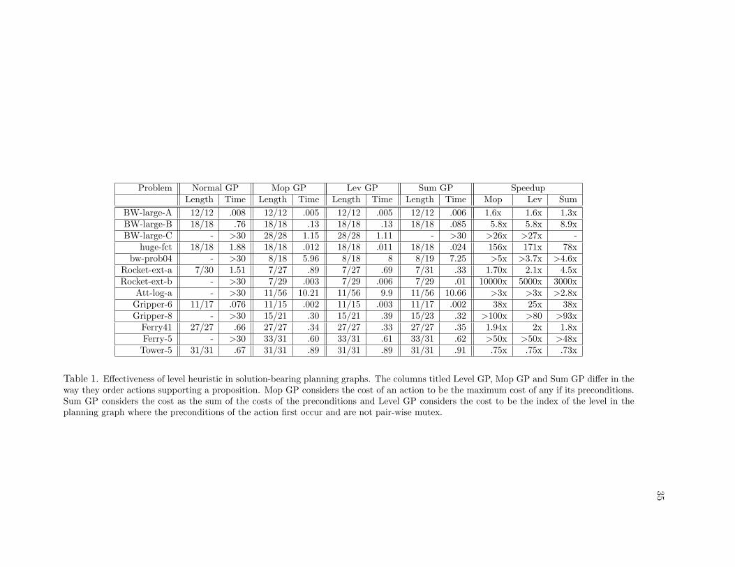
1. Effectiveness of level heuristic in solution-bearing planning graphs. The columns
titled Level GP, Mop GP and Sum GP differ in the way they order actions supporting
a proposition. Mop GP considers the cost of an action to be the maximum cost of
any if its preconditions. Sum GP considers the cost as the sum of the costs of
the preconditions and Level GP considers the cost to be the index of the level in
the planning graph where the preconditions of the action first occur and are not
pair-wise mutex. . . . . . . . . . . . . . . . . . . . . . . . . . . . . . . . . . . 35
2. Comparing the performance of AltAlt with STAN, a state-of-the-art Graph-
plan system, and HSP-r, a state-of-the-art heuristic state search planner. . 50
x

LIST OF FIGURES
Figure Page
1. Planning substrates . . . . . . . . . . . . . . . . . . . . . . . . . . . . . . . 11
2. Rover planning problem . . . . . . . . . . . . . . . . . . . . . . . . . . . . . 14
3. Partial rover state-space . . . . . . . . . . . . . . . . . . . . . . . . . . . . . 18
4. Forward-search algorithm . . . . . . . . . . . . . . . . . . . . . . . . . . . . 19
5. Execution of partial plan found by Forward-search . . . . . . . . . . . . . . 21
6. Backward-search algorithm . . . . . . . . . . . . . . . . . . . . . . . . . . . 23
7. The Rover planning graph example. To avoid clutter, we do not show the
no-ops and Mutexes. . . . . . . . . . . . . . . . . . . . . . . . . . . . . . . . 29
8. Architecture of AltAlt . . . . . . . . . . . . . . . . . . . . . . . . . . . . . . 38
9. Results in Blocks World and Logistics from AIPS-00 . . . . . . . . . . . . . 52
10. Results on trading heuristic quality for cost by extracting heuristics from
partial planning graphs. . . . . . . . . . . . . . . . . . . . . . . . . . . . . . 53
11. Architecture of AltAltp . . . . . . . . . . . . . . . . . . . . . . . . . . . . . . 60
12. AltAltp notation . . . . . . . . . . . . . . . . . . . . . . . . . . . . . . . . . 60
13. Node expansion procedure . . . . . . . . . . . . . . . . . . . . . . . . . . . . 63
14. After the regression of a state, we can identify the Pivot and the related set
of pairwise independent actions. . . . . . . . . . . . . . . . . . . . . . . . . . 64
15. Spar is the result of incrementally fattening the Pivot branch with the pair-
wise independent actions in O . . . . . . . . . . . . . . . . . . . . . . . . . . 64
16. PushUp procedure . . . . . . . . . . . . . . . . . . . . . . . . . . . . . . . . 67
17. Rearranging of the partial plan . . . . . . . . . . . . . . . . . . . . . . . . . 68
xi

Figure Page
18. Performance on Logistics (AIPS-00) . . . . . . . . . . . . . . . . . . . . . . 73
19. Performance on ZenoTravel (AIPS-02) . . . . . . . . . . . . . . . . . . . . . 76
20. AltAlt and Post-Processing vs. AltAltp (Zenotravel domain) . . . . . . . . . 77
21. Analyzing the effect of the PushUp procedure on the Logistics domain . . . 79
22. Plots showing the utility of using parallel planning graphs in computing the
heuristics, and characterizing the overhead incurred by AltAltp in serial do-
mains. . . . . . . . . . . . . . . . . . . . . . . . . . . . . . . . . . . . . . . . 80
23. Hierarchical overview of several types of complete and partial satisfaction
planning problems. . . . . . . . . . . . . . . . . . . . . . . . . . . . . . . . . 85
24. Rover domain problem . . . . . . . . . . . . . . . . . . . . . . . . . . . . . . 86
25. AltAltps architecture . . . . . . . . . . . . . . . . . . . . . . . . . . . . . . . 89
26. Cost function of at(waypoint1) . . . . . . . . . . . . . . . . . . . . . . . . . 90
27. Goal set selection algorithm. . . . . . . . . . . . . . . . . . . . . . . . . . . . 94
28. Modified rover example with goal interactions . . . . . . . . . . . . . . . . . 97
29. Multiple goal set selection algorithm . . . . . . . . . . . . . . . . . . . . . . 99
30. Interactions through actions . . . . . . . . . . . . . . . . . . . . . . . . . . . 105
31. Plots showing the total time and net benefit obtained by different PSP ap-
proaches . . . . . . . . . . . . . . . . . . . . . . . . . . . . . . . . . . . . . . 111
32. Graphical view of rover problem 11. . . . . . . . . . . . . . . . . . . . . . . 167
xii

CHAPTER 1
Introduction
Planning in the general case can be seen as the problem of finding a sequence of
actions that achieves a given goal from an initial situation of the world [Russell and Norvig,
2003]. Planning in fully observable, deterministic, finite, static and discrete domains is called
Classical Planning [Ghallab et al., 2004; Russell and Norvig, 2003; Kambhampati et al.,
1997], and although, real world problems may be far more complex than those represented
by classical planning, it has been shown that even this restrictive class of propositional
planning problems is PSPACE-complete in general [Bylander, 1994]. Therefore, one of the
main challenges in planning is the generation of heuristic metrics that can help planning
systems to scale up to more complex planning problems and domains. Such heuristic metrics
have to be domain-independent in the absence of control knowledge in order to work across
different plan synthesis algorithms and planning domains, which increases the complexity
of finding efficient and flexible estimates.
More formally speaking, a planning problem can be seen as a three-tuple P =
(Ω, G, I), where Ω represents the set of deterministic actions instantiated from the problem
description, G is a goal state, and I is the initial state of the problem. A plan ρ can be
seen as a sequence of actions a1, a2, ..., an which, when applied to the initial state I of the

2
problem, achieves the goal state G [Ghallab et al., 2004; Russell and Norvig, 2003]. Each
action ai ∈ Ω has a set of conditions that must be true for the action to be applicable, such
conditions are described in terms of a precondition list Prec(ai). The effects of the actions
Eff(ai) are described in two separate lists, an add list Add(ai) that specifies the conditions
that the action makes true, and a delete list Del(ai), which describes those conditions that
the action negates from the current state of the world.
One of the most efficient planning frameworks for solving large deterministic plan-
ning problems is state-space planning [Bonet et al., 1997; Bonet and Geffner, 1999;
Hoffmann and Nebel, 2001; Do and Kambhampati, 2001; Nguyen et al., 2002; Gerevini
and Serina, 2002], which explicitly searches in the space of world states using heuristics
to evaluate the goodness of them. The heuristic can be seen as estimating the num-
ber of actions required to reach a state, either from the goal G or the initial state I.
The main challenge of course is to design such heuristic function h that will rank the
states during search. Heuristic functions should be as informative as possible, as well
as cheap to compute. However, finding the correct trade-off could be as hard as solv-
ing the original problem [Ghallab et al., 2004]. Things get complicated by the fact that
subgoals comprising a goal state could have complex interactions. There are two kinds
of interactions among subgoals, negative and positive [Nguyen et al., 2002]. Negative in-
teractions happen when the achievement of a subgoal precludes the achievement of an-
other subgoal. Ignoring this type of interaction would normally underestimate the cost of
achievement. Positive interactions occur when the achievement of a subgoal reduces the
cost of achieving another one. Ignoring positive interactions would overestimate the cost
returned by the heuristic, making it inadmissible. In consequence, heuristics that make

3
strong assumptions (relaxations) about the independence of subgoals, often perform badly
in complex problems. In fact, taking into account such interactions to compute admissible
heuristics in state-space planning remains a challenging problem [Bonet and Geffner, 1999;
Nguyen et al., 2002].
This dissertation presents our work on heuristic planning. More specifically, our
research demonstrates the scalability of state-space planning techniques in problems where
their combinatorial complexity previously excluded state-space search for taking it into
consideration (e.g., parallel planning, over-subscription planning). The main contribution
of our work is the introduction of a flexible and effective heuristic framework that carefully
takes into account complex subgoals interactions, producing more informative heuristic
estimates. Our approach, based on planning graphs [Blum and Furst, 1997], computes
approximate reachability estimates to guide the search during planning. Furthermore, as
we will discuss later, our heuristic framework is flexible enough to be applied to any plan
synthesis algorithm.
This work will show first that the planning graph data structure of Graphplan is
an effective medium to automatically extract reachability information for any planning
problem. It will show then how to use such reachability information to develop distance-
based heuristics directly in the context of Graphplan. After that, this research will show that
planning graphs are also a rich source for deriving effective and efficient heuristics, more
sensitive to subgoals interactions, for controlling state-space search. In addition to this,
methods based on planning graphs to control the cost of computing the heuristics and limit
the branching factor of the search are also introduced. Extensions to our heuristic framework
are made to support the generation of parallel plans in state-space search [Sanchez and

4
Kambhampati, 2003a]. Our approach generates parallel plans online using distance-based
heuristics, and improves even further the quality of the solutions returned by using a plan
compression algorithm.
Finally, we will also show the applicability of our heuristic framework to cost-based
sensitive problems. More specifically, we will address the application of heuristic state-space
planning to partial satisfaction (over-subscription) planning problems. Over-subscribed
problems are those in which there are many more objectives than the agent can satisfy
given its resource limitations, constraints or goal interactions. Our approach introduces a
greedy algorithm to solve cost-sensitive partial satisfaction planning problems in the context
of state-space search, using mutex analysis to solve over-subscribed problems where goals
have complex interactions. We will present extensive empirical evaluation of the application
of our planning graph based techniques across different domains and problems.
Beyond the context of planner efficiency, and impressive results, our current work
can be best viewed as an important step towards the generation of heuristic metrics that
are informative as well as cost effective not only for state-space search but also for any other
planning framework. This work demonstrates then that planning graph based heuristics are
highly flexible, and successful for scaling up plan synthesis algorithms.
The remainder of this chapter highlights our specific research contributions and the
overall organization of this dissertation.
.

5
1.1. Specific Research Contributions
The contributions of this dissertation can be divided in two major directions. In
the first one, we demonstrate that the planning graph data structure from Graphplan is
a rich source for extracting very effective heuristics, as well as important related infor-
mation to control the cost of computing such heuristics and limit the branching factor of
the search. Specifically, we will show the effectiveness of such heuristics in the context
of regression state-space search by introducing two efficient planners that use them, Al-
tAlt and AltAltp.1 Part of AltAlt’s work has been presented at KBCS-2000 [Sanchez et
al., 2000], and has been also published by the Journal of Artificial Intelligence [Nguyen et
al., 2002]. AltAltp’s work has been presented at IJCAI-2003 [Sanchez and Kambhampati,
2003b], and it has been published by the Journal of Artificial Intelligence Research [Sanchez
and Kambhampati, 2003a]. The reachability information from the planning graph has also
been applied to the backward search of Graphplan itself. This work has been presented at
AIPS-2000 [Kambhampati and Sanchez, 2000].
In the second direction, we will show that state-space planning can be successfully
applied to more complex planning scenarios by adapting our heuristic framework. We will
introduce a greedy state-space search algorithm to solve Partial Satisfaction Cost-sensitive
(Over-subscription) problems. This time, our heuristic framework is extended to cope
with cost sensitive information. This work has developed two planning systems AltAltps
and AltWlt that solve over-subscription planning with respect to the PSP Net Benefit
1Preliminary work on AltAlt was presented by Xuanlong Nguyen at AAAI-2000 [Nguyen and Kambham-pati, 2000].

6
problem. 2 The work on AltAltps has been presented in WIPIS-2004 [van den Briel et al.,
2004b] and in AAAI-2004 [van den Briel et al., 2004a]. Extensions to AltAltps to handle
complex goal interactions and multiple goal selection was presented at ICAPS-2005 [Sanchez
and Kambhampati, 2005].
1.2. Thesis Organization
The next Chapter presents a brief background on automated planning and its rep-
resentation. We provide a description of classical planning, the specific planning substrate
that this dissertation mostly deals with. We also introduce state-space plan synthesis algo-
rithms, highlighting the need for heuristic support in planning.
In Chapter 3, we introduce the notion of distance-based heuristics in Graphplan.
We show how these estimations can naturally be extracted from planning graphs, and use
them to guide Graphplan’s own backward search. Then, we explain how we can further
extract more aggressive planning graph heuristics and apply them to drive regression state-
space search. We also show that planning graphs themselves are an effective medium for
controlling the cost of computing the heuristics and reducing the branching factor of the
search.
Next Chapter, we demonstrate the applicability of state-space search to parallel
planning by extending our heuristic framework. Our approach is sophisticated in the sense
that parallelizes partial plans online using planning graph estimations. Our empirical eval-
2Curious readers may advance to Chapter 5 for a description of PSP Net Benefit.

7
uation shows that our approach is an attractive tradeoff between quality and efficiency in
the generation of parallel plans.
Finally, Chapter 5 exposes state-space planning to Partial Satisfaction prob-
lems [Haddawy and Hanks, 1993], where the planning graph heuristics are adjusted to take
into account real execution costs of actions and goal utilities. This chapter also presents
techniques to account for complex goal interactions using mutex analysis from the planning
graph. Chapter 6 discusses related work, and Chapter 7 summarizes the contributions of
this dissertation and future directions.

CHAPTER 2
Background on Planning and State-space Search
Automated planning can be seen as the process of synthesizing goal-directed behav-
ior. In other words, planning is the problem of finding a course of actions that deliberatively
transforms the environment of an intelligent agent in order to achieve some predefined ob-
jectives. Automated planning not only involves action selection, but also action sequencing,
entailing during this process rational behavior. Therefore, one of the main motivations be-
hind automated planning is the design and development of autonomous intelligent agents
that can interact with humans [Ghallab et al., 2004].
There are many forms of planning given that there are many different problems in
which planning could be applied. In consequence, planning problems could be addressed us-
ing domain-specific approaches, in which each problem gets solved using a specific set of tech-
niques and control knowledge related to it. However, domain-specific planning techniques
are hard to evaluate and develop given that they are specific to a unique agent structure,
and in consequence, their applicability is very limited. For all these reasons, unless stated
otherwise, this dissertation is concerned in developing domain-independent planning tools
that can be applicable to a more general range of planning problems. Domain-independent
planners take as input an abstract general model of actions, and a problem definition, pro-

9
ducing a solution plan. Depending of the problem, a solution plan could be sets of actions
sequences, policies, action trees, task networks, variable assignments, etc.
Planning is hard, some of the main factors that increase planning complexity are
large search spaces, lack of heuristic guidance, problem decomposition and complex goal and
action interactions. However, plan synthesis algorithms have advanced enough to be useful
in a variety of applications. Including among these NASA space applications [RAX, 2000;
Jonsson et al., 2000; Ai-Chang et al., 2004], aviation (e.g, flight planning software), DoD
applications (e.g, mission planning), planning with workflows [Srivastava and Koehler,
2004], planning and scheduling integration [Kramer and Giuliano, 1997; Frank et al., 2001;
Smith et al., 2000; 1996; Chien et al., 2000], grid computing [Blythe et al., 2003], auto-
nomic computing [Ranganathan and Campbell, 2004; Srivastava and Kambhampati, 2005],
logistics applications and supply chain management (e.g. transportation, deployment, etc),
data analysis, process planning, factory automation, etc.
The success of plan synthesis algorithms in the last few years is mainly due to the
development of efficient and effective heuristics extracted automatically from the problem
representation, which help planning systems to improve their search control. The primary
goal of this dissertation is to show the impact of our work on this planning revolution by
demonstrating empirically and theoretically that state-space planning algorithms can scale
up to complex problems, when augmented with efficient and effective heuristics. Planning
graphs provide rich reachability information that can be used to derive estimates that can
be used across different planning problems.
The rest of this Chapter is organized as follows, in the next Section a brief back-
ground on the many complexities of planning is provided, putting special emphasis on the

10
substrate of planning that this research mostly deals with (i.e., classical planning) and its
representation. After that, state-space plan synthesis algorithms are presented, highlighting
their need for heuristic support in order to scale up to complex planning problems.
2.1. The Classical Planning Problem
The planning problem involves manipulation of the agent’s environment in an in-
telligent way in order to achieve a desired outcome. Under this scenario, the complex-
ity of plan synthesis is directly linked to the capabilities of the agent and the restric-
tions on the environment. This dissertation considers only environments that are fully
observable, static, propositional, finite and in which the agent’s execution of actions
are instantaneous (discrete) and deterministic. Plan synthesis under these conditions is
known as the classical planning problem [Russell and Norvig, 2003; Ghallab et al., 2004;
Kambhampati, 1997], see Figure 1 reproduced from [Kambhampati, 2004]:
• Fully observable: the environment is fully observable if the agent has complete and
perfect knowledge to identify in which state of the world it is.
• Static: The environment is static if only responds to the agent’s changes.
• Propositional: Planning states are represented with boolean state variables.
• Finite: The whole planning problem can be represented with a finite number of states.
• Deterministic: Each possible action of the agent, when applicable to a single state,
leads to a well defined other single state.

11
Figure 1. Planning substrates
• Instantaneous (Discrete): Agent’s actions do not have durations. They are instanta-
neous state transitions.
Although, classical planning appears to be restrictive for more real world prob-
lems, it is still computationally very hard, PSPACE-complete or worse [Erol et al., 1995;
Bylander, 1994; Ghallab et al., 2004]. We can see in Figure 1 some of these planning en-
vironments. Notice that a particular extension over instantaneous actions is when actions
have durations, but still the planning problem could remain classical (if the environment
is static, deterministic and fully observable). Some adaptations of the heuristics estimates
discussed in this research have been implemented to cope with these types of problems [Do
and Kambhampati, 2003; Bryce and Kambhampati, 2004].

12
2.2. Plan Representation
The classical planning problem involves selection of actions as well as sequencing
decisions to change the environment of the agent. Therefore, one way of representing the
classical planning problem is to use general models that reflect the nature of dynamic
systems. One such a model is a state-transition system [Dean and Wellman, 1991; Ghallab
et al., 2004]. A state-transition planning system can be seen as a 3-tuple Υ = (S, A, γ),
where:
• S is a finite set of states;
• A is a finite set of deterministic actions; and
• γ is ternary relation in terms of S x A x S, which represents the state-transition
function showing that there is a transition from state si to state sj with action ak.
A state-transition system Υ can be seen as a directed graph, where the states S
correspond to nodes in the graph, and actions in A correspond to the arcs in the graph,
labeling the transitions between the nodes. Under this representation, finding a plan in
deterministic environments is equivalent to finding paths in the graph corresponding to the
transition system. Transition system models are commonly called “explicit” models because
they explicit enumerate the set of all possible states and transitions. Unfortunately, such
description is impossible in large and complex planning problems. In general, factored
models are needed, in which the planning problem is more compactly represented, and in
which states and their transitions are computed on-the-fly. One of such representations

13
is based on State-variable models. Next subsection introduces one model based on binary
state-variables, which constitutes the most known representation for classical planning.
2.2.1. Binary State-variable Model. One of the most known representations for
classical planning is the Binary State-variable model. On this model, states of the world are
represented by binary state-variables. In other words, each state is a conjunction of logical
atoms (propositional literals) that can take true or false values. Under this representation,
actions are modeled as planning operators that change the truth values of the state literals,
they are in fact considered as state transformation functions. For the purposes of this work,
literals are completely ground and function free.
Most work in classical planning has followed the state-variable model using the
STRIPS representation [Fikes and Nilsson, 1971; Lifschitz, 1986]. In STRIPS, a planning
state is conformed of a conjunction of positive literals. For simplicity, we consider the
closed-world assumption [Russell and Norvig, 2003], meaning that any literals that are not
present in a particular state have false values. A planning problem using STRIPS is then
specified by:
• A complete initial state,
• A partially specified goal state, in which non-goal literals are not specified; and
• A set of ground actions. Each action is represented in terms of its preconditions,
which consist of a set of conditions (literals) that need to be true in the state for the
action to be executed; and a set of effects (positive as well as negative) that describes
how the state changes when the action gets executed.

14
Figure 2. Rover planning problem
The most accepted standard language to represent planning problems inspired by
the STRIPS representation is PDDL [Committee, 1998]. 1 In PDDL, planning problems
are usually described using two components. The first component describes the literals that
conform the planning domain, their types, any relations among them, and their values. It
also describes the literals that conform the initial state of the problem as well as the top
level goal state. The second component is an operator file that describes the skeleton for
the actions in terms of their parameters, preconditions, and effects. We can see in Figure 2
a problem from the Rover domain [Long and Fox, 2003], and in Example 2.2.1 a description
of it using the PDDL language.
Example 2.2.1
Suppose that we want to formulate a rover planning problem in which there are three
locations or waypoints (wp0, wp1, wp2), one rover (rover0), one store (store0), and one
lander (general). There are two types of samples (i.e., rock and soil). The problem is
to travel across different waypoints to collect the samples and send the data back to the
1The Planning Domain Definition Language

15
lander. We can see in Figure 2 that there are only three samples to collect, two in waypoint
one, and one in waypoint two. For this problem, we have the following PDDL description:
Rover problem.pddl
(define (problem roverExample) (:domain Rover)
(:objects general rover0 store0
wp0 wp1 wp2)
(:init
(visible wp0 wp1)
(visible wp1 wp0)
(visible wp0 wp2)
(visible wp2 wp0)
(visible wp1 wp2)
(visible wp2 wp1)
(rover rover0) (store store0) (lander general)
(waypoint wp0) (waypoint wp1) (waypoint wp2)
(atsoilsample wp1)
(atrocksample wp1) (atrocksample wp2)
(channelfree general) (at general wp0)
(at rover0 wp0) (available rover0)
(storeof store0 rover0) (empty store0)
(equippedforsoilanalysis rover0) (equippedforrockanalysis rover0)
(cantraverse rover0 wp0 wp1)
(cantraverse rover0 wp0 wp2)
(cantraverse rover0 wp2 wp1))
(:goal (and
(communicatedsoildata wp1)
(communicatedrockdata wp1)
(communicatedrockdata wp2))))
end Problem definition;
The second component is the domain file, which describes the operators that are
applicable in the planning problem. This file describes basically the dynamics of the plan-
ning domain by specifying the literals that each operator requires, and also those that they
affect. Here is a partial example on the rover domain:

16
Rover Domain.pddl
(:requirements :strips)
(:predicates (at ?x ?y) ...)
(:action navigate
:parameters ( ?x ?y ?z)
:precondition
(and (rover ?x) (waypoint ?y) (waypoint ?z)(at ?x ?y)
(cantraverse ?x ?y ?z) (available ?x)(visible ?y ?z))
:effect
(and (not (at ?x ?y)) (at ?x ?z)))
(:action samplesoil
:parameters ( ?x ?s ?p)
:precondition
(and (rover ?x) (store ?s) (waypoint ?p)
(at ?x ?p) (atsoilsample ?p) (empty ?s)
(equippedforsoilanalysis ?x) (storeof ?s ?x))
:effect
(and (not (empty ?s)) (not (atsoilsample ?p))
(full ?s) (havesoilanalysis ?x ?p)))
(:action communicatesoildata
:parameters (?r ?l ?p ?x ?y)
:precondition
(and (rover ?x) (lander ?l) (waypoint ?p) (waypoint ?x)
(waypoint ?y) (at ?r ?x) (at ?l ?y) (havesoilanalysis ?r ?p)
(visible ?x ?y) (available ?r) (channelfree ?l))
:effect
(communicatedsoildata ?p))
(:action drop
:parameters ( ?x ?y)
:precondition
(and (rover ?x) (store ?y) (storeof ?y ?x) (full ?y))
:effect
(and (not (full ?y)) (empty ?y)))
end Domain definition;
Once we have the domain and problem description in PDDL, they are used to com-
pute the set of ground actions that the planner manipulates in order to find a solution to
the problem. This step during the planning process is commonly called plan synthesis, and
there are a variety of planning algorithms that perform it. In the next Section, we briefly

17
discusses some of the most popular algorithms, putting special emphasis on state-space
search algorithms, in which our planning solutions are based.
2.3. Heuristic State-space Plan Synthesis Algorithms
Algorithms that search on the space of world states are maybe the most straightfor-
ward algorithms used to solve classical planning problems. In these algorithms, each state of
the world is represented through a node in a graph structure, and each arc in the graph corre-
sponds to a state transition carried out by the execution of a single action from the planning
domain. In consequence, in state-space planning each state is represented as a set of propo-
sitions (or subgoals). A plan on this representation would correspond to a path in the graph
that links the initial state of the problem to the goal state. We can see in Figure 3 a sub-
set of the search space unfolded from the initial state specified in Figure 2, and described
by Example 2.2.1. Notice that the initial and goal states are pointed out in the figure,
and specified by S0 = at(rover0,wp0), atrocksample(wp1), atsoilsample(wp1),
atrocksample(wp2), at(general,wp0),..., and G = communicatedsoildata(wp1),
communicatedrockdata(wp1), communicatedrockdata(wp2).
As mentioned before, a planning problem in state-space gets also represented as a
three-tuple P = (Ω, G, S0). We are given a complete initial state S0, a goal state G that
could be partially specified, and a set of deterministic actions Ω which are modeled as
state transformation functions. As mentioned earlier, each action a ∈ Ω has a precondition
list, add list and delete list (effects), denoted by Prec(a), Add(a), and Del(a), respectively.
The planning problem is concerned with finding a plan ρ, e.g a totally ordered sequence

18
Figure 3. Partial rover state-space

19
Algorithm ForwardSearch(S0, G,Ω)
S ← S0
ρ← ∅
loop
if(G ⊆ S) return ρ
Q← a|a ∈ Ω, and applicable in S
if(Q = ∅) return Failure
nondeterministally choose a ∈ Q
S ← Progress(S, a)
ρ← ρ.a
End ForwardSearch;
Figure 4. Forward-search algorithm
of actions in Ω,2 that when applied to the initial state S0 (and executed) will achieve the
goal G. Given the representation of the planning problem, there are two obvious ways of
implementing state-space planning. Forward-search and Backward-search.
2.3.1. Forward-search. Starts from the initial state S0, trying to find a state S′
that satisfies the top level goals G. In Forward search, we progress the state space through
the application of actions. An action a is said to be applicable to state S if Prec(a) ⊆ S.
The result of progressing an action a over S is defined using the following progression
function:
Progress(S, a) := (S ∪Add(a)) \Del(a) (2.1)
The states produced by the progression function 2.1 are consistent and complete
given that the initial state S0 is completely specified. However, heuristics have to be re-
computed at every new state during search, which could be very expensive. We can see in
Figure 4 a description of the Forward-search algorithm. It takes as input a planning prob-
2We will relax this restriction later in Chapter 4 when we consider parallel state-space planning.

20
lem P = (S0, G, Ω) specified in terms of the initial and goal states, and the set of actions in
the domain [Ghallab et al., 2004]. The algorithm returns a plan ρ if there is a solution, or
failure otherwise. The nondeterministic choice of the next state to progress in the algorithm
is usually manipulated heuristically. Otherwise, it would be impossible to search the large
state-space of complex planning problems. In progression, the heuristic function h over a
state S is the cost estimate of a plan that achieves G from that state. We could check
correctness of a plan ρ by progressing the initial state S0 through the sequence of actions
a ∈ ρ, checking that G is present in the final state of the sequence. The Forward-search
classical planning algorithm is sound and complete [Ghallab et al., 2004]
Example 2.3.1
As an example of how the Forward-search algorithms works, consider the
initial state S0 shown in Figure 2, and the domain description intro-
duced in our last example. It can be seen that the partial action se-
quence ρ = navigate(rover0,wp0,wp2), samplerock(rover0,store0,wp2),
communicaterockdata(rover0,general,wp2,wp2,wp0) , produces the resulting
state S′ = at(rover0,wp2), full(store0), haverockanalysis(rover0,wp2),
communicatedrockdata(wp2) if executed from S0, constituting the path represented in
the partial graph shown in Figure 5.
2.3.2. Backward-search. Although the Forward-search algorithm generates only
consistent states, the branching factor of its search can be quite large. The main reason for
this is that at each iteration the algorithm progresses all the actions in the domain that are

21
Figure 5. Execution of partial plan found by Forward-search

22
applicable to the current state. The problem is that many of these actions may not be even
relevant for achieving our goals, this is called the irrelevant action problem [Russell and
Norvig, 2003]. On the other hand, the Backward-search algorithm considers only relevant
actions to the current subgoal, making the search more goal oriented. An action is said
to be relevant to a current state, if it achieves at least one of the literals (subgoals) in it.
The idea with Backward-search is to start from the top-level goal definition, and apply
inverses of actions to produce pre-conditions. The algorithm stops when our current state
is subsumed by the initial state. More formally speaking, in backward state-space search,
an action a is said to be regressable to state S if:
• Action is relevant, Add(a) ∩ S 6= ∅, and;
• it is consistent, Del(a) ∩ S = ∅.
Then, the regression of S over an applicable action a is defined as:
Regress(S, a) := (S \Add(a)) ∪ Prec(a) (2.2)
The result of regressing a state S over an action a represents basically the set of goals
that still need to be achieved before the application of a, such that everything in S would
have been achieved once a is applied. We can see the overall description of the Backward
state-space search algorithm in Figure 6. The Backward-search algorithm is also sound and
complete [Pednault, 1987; Weld, 1994].
Even though the branching factor of Backward-search gets reduced to the application
of relevant actions, it can still be large. Moreover, Backward-search works on states that

23
Algorithm BackwardSearch(S0, G,Ω)
S ← G
ρ← ∅
loop
if(S ⊆ S0) return ρ
Q← a|a ∈ Ω, and regressable in S
if(Q = ∅) return Failure
nondeterministally choose a ∈ Q
S ← Regress(S, a)
ρ← a . ρ
End BackwardSearch;
Figure 6. Backward-search algorithm
are partially specified, producing more spurious states. Therefore, heuristic estimates are
also needed to speed up search. In regression, heuristic functions are computed only once
from the single initial state, representing the cost estimate of a plan that achieves a fringe
state S from the initial state S0.
2.4. Heuristic Support for State-space Planning
The efficiency and quality of state-space planners depend critically on the informed-
ness and admissibility of their heuristic estimators. The difficulty of achieving the desired
level of informedness and admissibility of the heuristic estimates is due to the fact that
subgoals interact in complex ways. As mentioned before, there are two kinds of subgoal
interactions: negative interactions and positive interactions. Negative interactions happen
when achieving one subgoal interferes with the achievement of some other subgoal. Ignor-
ing this kind of interactions would normally underestimate the cost, making the heuristic
uninformed. Positive interactions happen when achieving one subgoal also makes it easier
to achieve other subgoals. Ignoring this kind of interactions would normally overestimate

24
the cost, making the heuristic estimate inadmissible. For the rest of this section we will
demonstrate the importance of accounting for subgoal interactions in order to compute
more informed heuristic functions. We do so by examining the weakness of heuristics such
as those used by HSP-r [Bonet et al., 1997], which ignore these subgoal interactions.
The HSP-r planner is a regression state-space algorithm. The heuristic value h of a
state S is the estimated cost (number of actions) needed to achieve S from the initial state
S0. In HSP-r, the heuristic function h is computed under the assumption that the proposi-
tions constituting a state are strictly independent. Thus the cost of a state is estimated as
the sum of the cost for each individual proposition making up that state.
h(S)←∑
p∈S
h(p) (2.3)
Where the heuristic cost h(p) of an individual proposition p is computed using an
iterative procedure that is run to fixpoint as follows. Initially, p is assigned a cost of 0 if
it is in the initial state S0, and ∞ otherwise. For each action a ∈ Ω that adds p, h(p) is
updated as:
h(p)← minh(p), 1 + h(Prec(a)) (2.4)
The updates continue until the h values of all the individual propositions stabilize.
Because of the independence assumption, the sum heuristic turns out to be inadmissible
(overestimating) when there are positive interactions between subgoals. Sum heuristic is also
less informed (significantly underestimating) when there are negative interactions between
subgoals.

25
We can follow our working example 2.3.1 to see how these limitations affect
the sum heuristic. Suppose that we want to estimate the cost of achieving the state
S = communicatedrockdata(wp1), communicatedrockdata(wp2) from S0. Under the
independence assumption, each proposition would require only three actions (i.e., navigate,
sample and communicate data), having an overall cost of 6 for S. However, we can easily see
for this example, that goals are negatively interacting since we can not sample two objects
unless we drop one of them, and the rover can not be at two waypoints at the same time.
Ignoring these interactions for this particular example results in underestimating the real
cost for supporting S. We can see that extracting effective heuristic estimators to guide
state-space search is a crucial task, and one of the aims of this dissertation is to provide
a flexible heuristic framework that can make state-space planning scalable to more com-
plex planning problems. The next Chapter introduces planning graphs in the context of
Graphplan [Blum and Furst, 1997], setting the basis for our work in domain-independent
heuristics.

CHAPTER 3
Planning Graphs as a Basis for Deriving Heuristics
The efficiency of most plan synthesis algorithms and their solution quality depend
highly on the informedness and admissibility of their heuristic estimators. The difficulty
to improve such estimators is due to the fact that subgoals interact in complex ways. To
make computation tractable, such heuristic estimators make strong assumptions about the
independence of subgoals, resulting that most planners often thrash badly in problems where
there are strong interactions. Furthermore, also these independence assumptions make the
heuristics inadmissible affecting solution quality.
The Graphplan algorithm is good at dealing with problems where there are a lot
of interactions between actions and subgoals providing step optimality if a solution exists.
However, its main disadvantage is its backward search, which is exponential. Having to
exhaust the whole search space up to the solution bearing level is a big source of inefficiency.
Instead, in this chapter, we provide a way of successfully extracting heuristic estimators
from Graphplan and use them to guide effectively Graphplan’s own backward search and
state-space planning.
More specifically, the planning graph data structure from Graphplan can be seen as a
compact representation of the distance metrics that estimate the cost of achieving any propo-

27
sition in the planning graph from the initial state. This reachability information can then
be used to rank the subgoals and the actions being considered during Graphplan’s backward
search, improving its overall efficiency [Kambhampati and Sanchez, 2000]. Furthermore, we
will also show that these estimations can be combined to compute the cost of a specific state
by a regression planner. This will be demonstrated through AltAlt [Nguyen et al., 2002;
Sanchez et al., 2000],1 our approach that combines the advantages of Graphplan and state-
space search. AltAlt uses a Graphplan-style planner to generate a polynomial time planning
data structure, which will be used to generate effective state-space search heuristics [Nguyen
and Kambhampati, 2000; Nguyen et al., 2002]. These heuristics are then used to control
the search engine of AltAlt.
In the next sections, we introduce Graphplan and explain how distance-based heuris-
tics are generated from its planning graph data structure. We also show how these metrics
are used to improve Graphplan’s own backward search. Then, we extend our basic distance-
based metrics to state-space search. First, we discuss the architecture of our approach
AltAlt, and then we discuss the extensions to our heuristics to take into account complex
subgoal interactions. The final section presents an empirical evaluation of our heuristic
state-space planning framework.
3.1. The Graphplan Algorithm
One of the most successful algorithms implemented to solve classical planning prob-
lems is Graphplan of Blum and Furst [Blum and Furst, 1997]. The Graphplan algorithm can
1Preliminary work in AltAlt was done by Xuanlong Nguyen [Nguyen and Kambhampati, 2000].

28
be understood as a “disjunctive” version of the forward state-space planners [Kambhampati
et al., 1997].
The Graphplan algorithm alternates between two phases. A forward phase where
a polynomial time data structure, called “planning graph” is incrementally expanded, and
a backward phase where such structure is searched to extract a valid plan. The planning-
graph (see Figure 7) consists of two alternating structures, called “proposition lists” and
“action lists.” Figure 7 shows a partial planning-graph structure corresponding to the rover
Example 2.2.1. We start with the initial state as the zeroth level proposition list. Given
a k level planning graph, the extension of structure to level k + 1 involves introducing all
actions whose preconditions are present in the kth level proposition list. In addition to
the actions given in the domain model, we consider a set of dummy “persist” actions (no-
ops), one for each condition in the kth level proposition list (represented as dashed lines
in Figure 7). A “noopq” action has q as its precondition and q as its effect. Once the
actions are introduced, the proposition list at level k + 1 is constructed as just the union
of the effects of all the introduced actions. Planning-graph maintains the dependency links
between the actions at level k + 1 and their preconditions in level k proposition list and
their effects in level k + 1 proposition list. The planning-graph construction also involves
computation and propagation of “mutex” constraints. The propagation starts at level 1,
with the actions that are statically interfering with each other (i.e., their preconditions and
effects are inconsistent) labeled mutex. Mutexes are then propagated from this level forward
by using two simple propagation rules.

29
Figure 7. The Rover planning graph example. To avoid clutter, we do not show the no-ops and Mutexes.

30
1. Two propositions at level k are marked mutex if all actions at level k that support
one proposition are mutex with all actions that support the second proposition.
2. Two actions at level k + 1 are mutex if they are statically interfering or if one of the
propositions (preconditions) supporting the first action is mutually exclusive with one
of the propositions supporting the second action.
Notice that we have not included the mutex information in the graph of Fig-
ure 7 to avoid clutter, but we can easily see that the actions navigate(rover0,Wp0,Wp2)
and navigate(rover0,Wp0,Wp1) are statically interfering, in consequence the facts
at(rover0,Wp1) and at(rover0,Wp2) are mutex because all actions supporting them are
mutex to each other. In our current example from Figure 7, the goals are first present at
level three of the graph. However, even though it has not be shown, they are all mutexes
to each other. It is not until level five in the graph when they become free mutex.
The backward phase of Graphplan involves checking to see if there is a subgraph
from a k level planning-graph that corresponds to a valid solution to the problem. This
involves starting with the propositions corresponding to goals at level k (if all the goals are
not present, or if they are present but a pair of them are marked mutually exclusive, the
search is abandoned right away, and planning-graph is grown another level). For each of the
goal propositions, we then select an action from the level k action list that supports it, such
that no two actions selected for supporting two different goals are mutually exclusive (if they
are, we backtrack and try to change the selection of actions). At this point, we recursively
call the same search process on the k − 1 level planning-graph, with the preconditions of

31
the actions selected at level k as the goals for the k − 1 level search. The search succeeds
when we reach level 0 (corresponding to the initial state).
Graphplan’s backward search phase can be seen as a CSP problem. Specifically, a
dynamic constraint satisfaction problem [Mittal and Falkenhainer, 1990], where the propo-
sitions in the planning graph can be seen as CSP variables, and the actions supporting them
can be seen as their values. The constraints get specified by the mutex relations [Do and
Kambhampati, 2000; Lopez and Bacchus, 2003]. The next section introduces the notion of
reachability in the context of Graphplan itself, and show how this reachability analysis can
be used to develop distance-based estimates to improve Graphplan’s own backward search.
Following sections will demonstrate the application of domain independent planning graph
based heuristics to state-space planning.
3.2. Introducing the Notion of Heuristics and their Use in Graphplan
The plan synthesis algorithms explored in the previous chapter are effective in finding
solutions to planning problems. However, they all suffer from the combinatorial complexity
of the problems they try to solve. In consequence, one of the main directions in recent
years by the planning community has been the development of heuristic search control to
significantly scale up plan synthesis.
We can see in the descriptions of the algorithms presented in Section 2.3 that they
traverse the search space non-deterministically. In order to improve their node selection,
a function would be needed to select more deterministically those nodes that look more
promising during search from a set of candidates. Such functions are commonly called
32
heuristics, and most of the times are abstract solutions to relaxed problems that are used
to prioritize our original choices during search. As we can see, the main objective of a
heuristic function is to guide the search of the problem in the most promising direction
in order to improve the overall efficiency and scalability of the system. As we saw in
Section 2.4, finding accurate heuristic estimates that take into account subgoal interactions
is very important, given that even the smaller problems could be intractable in the worst
case.
3.2.1. Distance-based Heuristics for Graphplan. As mentioned earlier, pre-
vious work has demonstrated the connections between the backward search of Graphplan
and (dynamic) CSP problems [Mittal and Falkenhainer, 1990; Kambhampati et al., 1997;
Weld et al., 1998]. More specifically, the propositions in the planning graph can be seen
as CSP variables, while the actions supporting them can be seen as their domain of val-
ues. Constraints are then represented by the mutex relations in the graph. Given these
relations, the order in which the backward search considers the (sub)goals propositions for
assignment (i.e., variable ordering heuristic), and the order in which actions are chosen to
support those (sub)goals (i.e., value ordering heuristic) can have a significant impact in
Graphplan’s performance.
Our past work from [Kambhampati and Sanchez, 2000] has demonstrated that the
traditional variable and value ordering heuristics from CSP literature do not work well in
the context of Graphplan’s backward search. We then present a family of variable and
value-ordering heuristics that are based on the difficulty of achieving a subgoal from the
initial state. The degree of difficulty of achieving a single proposition is quantified by the

33
index of the earliest level of the planning graph in which that proposition first appears.
In other words, the intuition behind the distance-based heuristics is to choose goals based
on the “distance” of those goals from the initial state, where distance is interpreted as the
number of actions required to go from the initial state to the goal state. It turns out that we
can obtain the distances of various goal propositions through the planning graph structure.
The main idea is:
Propositions are ordered for assignment in decreasing value of their levels. Ac-
tions supporting a proposition are ordered for consideration in increasing value
of their costs (see below).
Where:
The level of a proposition p, lev(p) is defined as the earliest level l of the planning
graph that contains p.
These heuristics can be seen as using a “hardest to achieve goal (variable) first/easiest
to support action(value) first” idea, where hardness is measure in terms of the level of the
propositions. Consider the planning graph in Figure 7, the level of the top level goals is 3,
while the level of full(store0) is 2, and that of at(rover0,wp0) is 0. This propagation
is easy to compute in the planning graph. To support value ordering, we need to define the
cost of an action a supporting a proposition p. We have three different alternatives, all of
them based on the level information from the planning graph [Kambhampati and Sanchez,
2000]:
Mop heuristic: The cost of an action is the maximum of the cost (distance) of its pre-
conditions. For example in Figure 7 the cost of samplerock(rover0,store0,wp2) is

34
1, since all of its preconditions appear at level 1. This heuristic is defined as:
CostMop(a) = maxp∈Prec(a)lev(p) (3.1)
Sum heuristic: The cost of an action is the sum of the costs of the individual propositions
making up that action’s precondition list, namely:
CostSum(a) =∑
p∈Prec(a)
lev(p) (3.2)
Consequently, in Figure 7 the cost of samplerock(rover0,store0,wp2) would be 3.
Level heuristic: The cost of an action is the first level at which the set of its preconditions
is present in the graph without being any of them mutex with each other.2 Following
the same example from Figure 7 the cost of samplerock(rover0,store0,wp2) is 1
because its preconditions are non mutex at that level. The heuristic can be described
as:
CostLev(a) = lev(Prec(a)) (3.3)
These simple heuristics extracted from the planning graph and the notion of level
form the basis for building more powerful heuristics that will be applied to more complex
planning frameworks discussed in this dissertation.
2The Level heuristic of an action a is just the level in the planning graph where a first occurs.
35
Problem Normal GP Mop GP Lev GP Sum GP SpeedupLength Time Length Time Length Time Length Time Mop Lev Sum
BW-large-A 12/12 .008 12/12 .005 12/12 .005 12/12 .006 1.6x 1.6x 1.3xBW-large-B 18/18 .76 18/18 .13 18/18 .13 18/18 .085 5.8x 5.8x 8.9xBW-large-C - >30 28/28 1.15 28/28 1.11 - >30 >26x >27x -
huge-fct 18/18 1.88 18/18 .012 18/18 .011 18/18 .024 156x 171x 78xbw-prob04 - >30 8/18 5.96 8/18 8 8/19 7.25 >5x >3.7x >4.6x
Rocket-ext-a 7/30 1.51 7/27 .89 7/27 .69 7/31 .33 1.70x 2.1x 4.5xRocket-ext-b - >30 7/29 .003 7/29 .006 7/29 .01 10000x 5000x 3000x
Att-log-a - >30 11/56 10.21 11/56 9.9 11/56 10.66 >3x >3x >2.8xGripper-6 11/17 .076 11/15 .002 11/15 .003 11/17 .002 38x 25x 38xGripper-8 - >30 15/21 .30 15/21 .39 15/23 .32 >100x >80 >93x
Ferry41 27/27 .66 27/27 .34 27/27 .33 27/27 .35 1.94x 2x 1.8xFerry-5 - >30 33/31 .60 33/31 .61 33/31 .62 >50x >50x >48xTower-5 31/31 .67 31/31 .89 31/31 .89 31/31 .91 .75x .75x .73x
Table 1. Effectiveness of level heuristic in solution-bearing planning graphs. The columns titled Level GP, Mop GP and Sum GP differ in theway they order actions supporting a proposition. Mop GP considers the cost of an action to be the maximum cost of any if its preconditions.Sum GP considers the cost as the sum of the costs of the preconditions and Level GP considers the cost to be the index of the level in theplanning graph where the preconditions of the action first occur and are not pair-wise mutex.

36
3.3. Evaluating the Effectiveness of Level-based Heuristics in Graphplan
We implemented the three level-based heuristics discussed in this chapter for Graph-
plan’s backward search, and evaluated their performance as compared to normal Graph-
plan. Our extensions were based on the version of Graphplan implementation bundled in
the Blackbox system [Kautz and Selman, 1999], which in turn was derived from Blum &
Furst’s original implementation [Blum and Furst, 1997]. Table 1 shows the results on some
standard benchmark problems. The columns titled “Mop GP”, “Lev GP” and “Sum GP”
correspond respectively to Graphplan armed with the CostMop, CostLev, and CostSum
heuristics for variable and value ordering. Cpu time is shown in minutes. For our Pen-
tium Linux machine with 256 Megabytes of RAM.3 The table compares the effectiveness
of standard Graphplan (with noops-first heuristic [Kambhampati and Sanchez, 2000]), and
Graphplan with our three level-based heuristics in searching the planning graph containing
minimum length solution. As can be seen, the final level search can be improved by 2 to 4
orders of magnitude with the level-based heuristics.
Empirical results demonstrate that these heuristics could speedup backward search
by several orders in solution-bearing planning graphs. Our heuristics, while quite simple,
are nevertheless significant in that previous attempts to devise effective variable ordering
techniques for Graphplan’s search have not been successful.
3For an additional set of experiments see [Kambhampati and Sanchez, 2000].

37
3.4. AltAlt: Extending Planning Graph Based Heuristics to State-space
Search
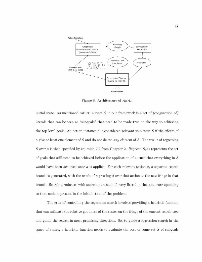
As mentioned earlier, AltAlt system is based on a combination of Graphplan and
heuristic state-space search technology. The high-level architecture of AltAlt is shown in
Figure 8. The problem specification and the action template description are first fed to a
Graphplan-style planner, which constructs a planning graph for that problem in polynomial
time. We use the publicly available STAN implementation [Long and Fox, 1999] for this
purpose as it provides a highly memory efficient implementation of the planning graph
construction phase. This planning graph structure is then fed to a heuristic extractor
module that is capable of extracting a variety of effective and admissible heuristics, based
on the theory that we have developed in our work [Nguyen and Kambhampati, 2000; Nguyen
et al., 2002], and that we will discuss in the next section. This heuristic, along with the
problem specification, and the set of ground actions in the final action level of the planning
graph structure are fed to a regression state search planner. The regression planner code is
adapted from HSP-r [Bonet and Geffner, 1999].
To explain the operation of AltAlt at a more detailed level, we need to provide some
further background on its various components. We shall start with the regression search
module. As introduced in Section 3.4, regression search is the process of searching in the
space of potential plan suffixes. The suffixes are generated by starting with the goal state
and regressing it over the set of relevant action instances from the domain. The resulting
states are then (non-deterministically) regressed again over relevant action instances, and
this process is repeated until we reach a state (set of subgoals) which is satisfied by the
38
Action Templates
Problem Spec (Init, Goal state)
Solution Plan
Graphplan Plan Extension Phase
(based on STAN)
Planning Graph Extraction of
Heuristics
Heuristics Actions in the
Last Level
Regression Planner (based on HSP-R)
Figure 8. Architecture of AltAlt
initial state. As mentioned earlier, a state S in our framework is a set of (conjunction of)
literals that can be seen as “subgoals” that need to be made true on the way to achieving
the top level goals. An action instance a is considered relevant to a state S if the effects of
a give at least one element of S and do not delete any element of S. The result of regressing
S over a is then specified by equation 2.2 from Chapter 2. Regress(S, a) represents the set
of goals that still need to be achieved before the application of a, such that everything in S
would have been achieved once a is applied. For each relevant action a, a separate search
branch is generated, with the result of regressing S over that action as the new fringe in that
branch. Search terminates with success at a node if every literal in the state corresponding
to that node is present in the initial state of the problem.
The crux of controlling the regression search involves providing a heuristic function
that can estimate the relative goodness of the states on the fringe of the current search tree
and guide the search in most promising directions. So, to guide a regression search in the
space of states, a heuristic function needs to evaluate the cost of some set S of subgoals

39
(comprising a regressed state), from the initial state–in terms of the length of the plan
needed to achieve them from the initial state.
The search algorithm used in AltAlt is similar to that used in HSP-r [Bonet and
Geffner, 1999]–it is a hybrid between greedy depth first and a weighted A* search. It goes
depth-first as long as the heuristic cost of any of the children states is lower than that of
the current state. Otherwise, the algorithm resorts to a weighted A* search to select the
next node to expand. In this latter case, the evaluation function used to rank the nodes
is f(S) = g(S) + w ∗ h(S), where g(S) is the accumulated cost (number of actions when
regressing from the goal state), h(S) is the heuristic value for a given state, and w is a
weight parameter set to 5.4
We now discuss how distance-based heuristics can be computed from the planning
graphs, which, by construction, provide optimistic reachability estimates.
3.5. Extracting Effective Heuristics from the Planning Graph
Normally, the planning graph data structure supports “parallel” plans–i.e., plans
where at each step more than one action may be executed simultaneously. Since we want
the planning graph to provide heuristics to the regression search module of AltAlt, which
generates sequential solutions, we first make a modification to the algorithm so that it
generates a “serial planning graph.” A serial planning graph is a planning graph in which,
in addition to the normal mutex relations, every pair of non-noop actions at the same
level are marked mutex. These additional action mutexes propagate to give additional
4For the role of w in search see [Korf, 1993]

40
propositional mutexes. Finally, a planning graph is said to level-off when there is no
change in the action, proposition and mutex lists between two consecutive levels.
The critical asset of the planning graph, for our purposes, is the efficient marking an
propagation of mutex constraints during the expansion phase. A mutex relation is called
static (or “persistent”) if it remains a mutex up to the level where the planning graph levels
off. A mutex relation is called dynamic (or level specific) if it is not static.
Based on the above, the following properties can be easily verified:
1. The number of actions required to achieve a pair of propositions is no less than the
index of the smallest proposition level in the planning graph in which both propositions
appear without a mutex relation.
2. Any pair of propositions having a static mutex relation between them can never be
true together.
3. The set of actions present in the level where the planning graph levels off contains all
actions that are applicable to states reachable from the initial state.
These observations give a rough indication as how the information in the leveled
planning graph can be used to guide state-space search planners. The first observation
shows that the level information in the planning graph can be used to estimate the cost of
achieving a set of propositions. Furthermore, the set of dynamic propositional mutexes help
to get finer distance estimates. The second observation allows us to prove that certain world
states are unreachable from the initial state pruning the search space. The third observation
shows a way of extracting a finer (smaller) set of applicable actions to be considered by the
regression search.

41
We will assume for now that given a problem, the Graphplan module of AltAlt is
used to generate and expand a serial planning graph until it levels off. (As we shall see
later, we can relax the requirement of growing the planning graph to level-off, if we can
tolerate a graded loss of informedness of heuristics derived from the planning graph.) We
will start with the notion of level of a proposition that was introduced informally before:
Definition 1 (Level). Given a proposition p, lev(p) is the index of the first level in the
leveled serial planning graph in which p first appeared.
The intuition behind this definition is that the level of a literal p in the planning
graph provides a lower bound on the number of actions required to achieve p from the initial
state. Following these observations, we can arrive to our first planning graph distance-based
heuristic [Nguyen et al., 2002; Sanchez et al., 2000]:
Heuristic 1 (Max heuristic). hmax(S) := maxp∈S lev(p)
The hmax heuristic is admissible, however, is not very informed as it grossly under-
estimates the cost of achieving a given state [Nguyen et al., 2002]. Our second heuristic
estimates the cost of a set of subgoals by adding up their levels:
Heuristic 2 (Sum heuristic). hsum(S) :=∑
p∈S lev(p)
The sum heuristic is very similar to the greedy regression heuristic used in UN-
POP [McDermott, 1999] and the heuristic used in the HSP planner [Bonet et al., 1997].
Its main limitation is that the heuristic makes the implicit assumption that all the sub-
goals (elements of S) are independent. Sum heuristic is neither admissible nor particularly

42
informed. Specifically, since subgoals can be interacting negatively (in that achieving one
winds up undoing progress made on achieving the others), the true cost of achieving a pair
of subgoals may be more than the sum of the costs of achieving them individually. This
makes the heuristic inadmissible. Similarly, since subgoals can be positively interacting in
that achieving one winds up making indirect progress towards the achievement of the other,
the true cost of achieving a set of subgoals may be lower than the sum of their individual
costs. To develop more effective heuristics, we need to consider both positive and nega-
tive interactions among subgoals in a limited fashion. We start taking into account more
interactions by considering the notion of level of a set of propositions:
Definition 2 (Set Level). Given a set S of propositions, lev(S) is the index of the first
level in the leveled serial planning graph in which all propositions in S appear and are non-
mutexed with one another (If S is a singleton p, then lev(S) = lev(p)). If no such level exists
and the planning graph has been grown to level-off then lev(S) = ∞. Or, lev(S) = l + 1,
where l is the index of the last level that the planning graph has been grown to (i.e not until
level-off).
Leading us to our next heuristic:
Heuristic 3 (Set-level heuristic). hlev(S) := lev(S)
It is easy to see that set-level heuristic is admissible. Secondly, it can be significantly
more informed than the max heuristic, because the max heuristic is only equivalent to the
level that a single proposition first comes into the planning graph. Thirdly, a by-product of
the set-level heuristic is that it is easy to compute and effective since we already have the
static and dynamic mutex information from the planning graph.

43
However, Set-level heuristics is not perfect. It tends to be too conservative and often
underestimates the real cost in domains with many independent subgoals [Nguyen et al.,
2002]. To overcome these limitations, two families of heuristics have been implemented
that take into account subgoals interactions, “partition-k” heuristics and “adjusted-sum”
heuristics [Nguyen and Kambhampati, 2000; Nguyen et al., 2002].
Partition-k heuristics:
The Partition-k heuristics attempts to improve and generalize the set-level heuristic
using the sum heuristic idea. Specifically, it estimates the cost of a set in terms of the
costs of its partitions. When the subgoals are relatively independent, the summation of the
cost of each individual gives a much better estimate, whereas the graph level value of the
set tends to underestimate significantly. To avoid this problem and at the same time keep
track of the interaction between subgoals, we want to partition the set S of propositions
into subsets, each of which has k elements: S = S1 ∪ S2... ∪ Sm (if k does not divide |S|,
one subset will have less than k elements), and then apply the set-level heuristic value on
each partition. Ideally, we want a partitioning such that elements within each subset Si
may be interacting with each other, but the subsets are independent (i.e non-interacting)
of each other. By interacting we mean the two propositions form either a pair of dynamic
(level-specific) or static mutex in the planning graph. These notions are formalized by the
following definitions.
Definition 3. The (binary) interaction degree δ between two propositions p1 and p2 is
defined as: δ(p1, p2) = lev(p1, p2)−maxlev(p1), lev(p2).

44
When p1 and p2 are dynamic mutex, δ(p1, p2) > 0 but lev(p1, p2) <∞. When p1
and p2 are static mutex, lev(p1, p2) = ∞. Since we only consider propositions that are
present in the planning graph, i.e maxlev(p1), lev(p2) < ∞, it follows that δ(p1, p2) > 0
as well. When p1 and p2 are neither type of mutex, lev(p1, p2) = maxlev(p1), lev(p2),
thus δ(p1, p2) = 0.
Definition 4. Two propositions p and q are interacting with each other if and only if
δ(p, q) > 0. Two sets of propositions S1 and S2 are not interacting with each other if no
proposition in S1 is interacting with a proposition in S2.
Following our definitions, we are ready to state our next heuristics:
Heuristic 4 (Partition-k heuristic).
hpart−k(S) :=∑
Silev(Si), where S1, ..., Sm are k-sized partitions of S.5
Adjusted-sum heuristics:
The second family of heuristics, called “adjusted sum” heuristics attempt to improve
the hsum heuristic 2 using the set-level idea 3. Specifically, it starts explicitly from the hsum
heuristic and then considers adding the positive and negative interactions among subgoals
that can be extracted from the planning graph’s level information. Since fully accounting for
either type of interaction alone can be as hard as the planning problem itself, we circumvent
this difficulty by using partial relaxation assumption on the subgoal interactions. Namely,
we ignore one type of subgoal interaction in order to account for the other, and then combine
them both together.
5For a deeper analysis on this class of heuristics see [Nguyen et al., 2002]

45
We start with the assumption that all propositions are independent. Remember that
this is a property of the hsum heuristic. We assume that there are no positive interactions,
but there are negative interactions among the propositions. This can be computed using
the interaction degree among propositions in a set S, which is no more than an extension
of Definition 3.
Definition 5. The interaction degree among propositions in a set S is:
∆(S) = hlev(S)− hmax(S)
We can easily see that when there are no negative interactions among the subgoals
hlev(S) = hmax(S). So, our following heuristics gets formulated as:
Heuristic 5 (Adjusted-sum heuristic). hadjsum(S) := hsum(S) + ∆(S)
As mentioned earlier, hsum accounts for the cost of achieving S under the indepen-
dence assumption, while ∆(S) accounts for the additional cost incurred by the negative
interactions.
We can improve the heuristic estimators of hadjsum(S) by replacing its first term
with another estimate that takes into account positive interactions. This is done by another
heuristic, which we called hadjsum2M (S).
The basic idea of hAdjSum2M is to adjust the sum heuristic to take positive as well
as negative interactions into account. This heuristic approximates the cost of achieving the
subgoals in some set S as the sum of the cost of achieving S, while considering positive
interactions and ignoring negative interactions, plus the penalty for ignoring the negative

46
interactions. The first component can be computed as the length of a “relaxed plan”
for supporting S, which is extracted by ignoring all the mutex relations. The relaxed
plan is computed by regressing S over an applicable action as, obtaining the state S′ =
Regress(S, as). Getting the following recurrent relation:
relaxP lan(S) = 1 + relaxP lan(S′) (3.4)
This regression accounts for the positive interactions in the state S given that by
subtracting the effects of as, any propositions that are co-achieved will not count in the cost
computation. The recursive application of the last equation is bounded by the final level
of the planning graph, and it will eventually reduce to a state S0 where each proposition
q ∈ S0 is also in the initial state I.
To approximate the penalty induced by the negative interactions alone, we proceed
to use the binary degree of interaction among any pair of propositions from Definition 3.
We want to use the δ(p, q) values to characterize the amount of negative interactions present
among the subgoals of a given set S. If all subgoals in S are pair-wise independent, clearly,
all δ values will be zero, otherwise each pair of subgoals in S will have a different value. The
largest such δ value among any pair of subgoals in S is used as a measure of the negative
interactions present in S in the heuristic hAdjSum2M . In summary, we have
Heuristic 6 (Adjusted heuristic 2M). hAdjSum2M (S) := length(relaxP lan(S)) +
maxp,q∈S δ(p, q)

47
The analysis in [Nguyen and Kambhampati, 2000; Nguyen et al., 2002] shows that
this is one of the more robust heuristics in terms of both solution time and quality. This is
thus the default heuristic used in AltAlt.6
3.6. Controlling the Cost of Computing the Heuristics
Although planning graph construction is a polynomial time operation, it does lead
to a relatively high time and space consumption in many problems. The main issues are the
sheer size of the planning graph, and the cost of marking and managing mutex relations.
Fortunately, however, there are several possible ways of keeping the heuristic computation
cost in check. To begin with, one main reason for basing AltAlt on STAN rather than other
Graphplan implementations is that STAN provides a particularly compact and efficient
planning graph construction phase. In particular, as described in [Long and Fox, 1999],
STAN exploits the redundancy in the planning graph and represents it using a very compact
bi-level representation. Secondly, STAN uses efficient data structures to mark and manage
the “mutex” relations.
While the use of STAN system reduces planning graph construction costs signifi-
cantly, heuristic computation cost can still be a large fraction of the total run time. Thank-
fully, however, by trading off heuristic quality for reduced cost, we can aggressively limit
the heuristic computation costs. Specifically, in the previous section, we discussed the ex-
traction of heuristics from a full leveled planning graph. Since AltAlt does not do any
search on the planning graph directly, there is no strict need to use the full leveled graph to
6See [Nguyen et al., 2002] for an extensive presentation of these heuristics and their variations.

48
preserve completeness. Informally, any subgraph of the full leveled planning graph can be
gainfully utilized as the basis for the heuristic computation. There are at least three ways
of computing a smaller subset of the leveled planning graph:
1. Grow the planning graph to some length that is less than the length where it levels
off. For example, we may grow the graph until the top level goals of the problem are
present without any of them having mutex relations.
2. Spend only limited time on marking mutexes on the planning graph.
3. Introduce only a subset of the “applicable” actions at each level of the planning graph.
For example, we can exploit the techniques such as RIFO [Kohler et al., 1997] and
identify a subset of the action instances in the domain that are likely to be “relevant”
for solving the problem.
Any combination of the above three techniques can be used to limit the space and
time resources expended on computing the planning graph. What is more, it can be shown
that the admissibility and completeness characteristics of the heuristic will remain unaf-
fected as long as we do not use the third approach. Only the informedness of the heuristic
is affected. We shall see later in this chapter that in many problems the loss of informedness
is more than offset by the improved time and space costs of the heuristic.
3.7. Limiting the Branching Factor of the Search Using Planning Graphs
The preceding chapters focused on the use of the planning graphs for computing
the heuristics in AltAlt. However, from Figure 8, we can see that the planning graph is

49
also used to pick the action instances considered for expanding the regression search tree.
The advantages of using the action instances from the planning graph are that in many
domains there is a prohibitively large number of ground action instances, only a very small
subset of which are actually applicable on a given state reachable from the initial state.
Using all such ground actions in regression search can significantly increase the cost of node
expansion (and may, on occasion, lead the search down the wrong paths). In contrast, the
action instances present in the planning graph are more likely to be applicable in states
reachable from the initial state.
The simplest way of picking action instances from the planning graph is to consider
all action instances that are present in the final level of the planning graph. If the graph
has been grown to level off, it can be proved that limiting regression search to this subset
of actions is guaranteed to preserve completeness. A more aggressive selective expansion
approach, that we call PACTION, involves the following. Suppose that we are trying to expand
a state S in the regression search, then only the set of actions appearing in the action level
lev(S) (i.e., the index of the level of the planning graph at which the propositions in set S
first appear without any pair-wise mutex relations between them) is considered to regress
the state S. The intuition behind PACTION strategy is that the actions in level lev(S)
comprise the actions that are likely to achieve the subgoals of S in the most direct way
from the initial state. While this strategy may in principle result in the incompleteness
of the search (for example, some actions needed for the solution plan could appear much
later in the graph, at levels l > lev(S)), we have not yet come across a single problem
instance in which our strategy fails to find a solution that can be found considering the full

50
STAN3.0 HSP-r HSP2.0 AltAlt(AdjSum2M)
Problem Time Length Time Length Time Length Time Length
gripper-15 - - 0.12 45 0.19 57 0.31 45
gripper-20 - - 0.35 57 0.43 73 0.84 57
gripper-25 - - 0.60 67 0.79 83 1.57 67
gripper-30 - - 1.07 77 1.25 93 2.83 77
tower-3 0.04 7 0.01 7 0.01 7 0.04 7
tower-5 0.21 31 5.5 31 0.04 31 0.16 31
tower-7 2.63 127 - - 0.61 127 1.37 127
tower-9 108.85 511 - - 14.86 511 48.45 511
8-puzzle1 37.40 31 34.47 45 0.64 59 0.69 31
8-puzzle2 35.92 30 6.07 52 0.55 48 0.74 30
8-puzzle3 0.63 20 164.27 24 0.34 34 0.19 20
8-puzzle4 4.88 25 1.35 26 0.46 42 0.41 24
aips-grid1 1.07 14 - - 2.19 14 0.88 14
aips-grid2 - - - - 14.06 26 95.98 34
mystery2 0.20 9 84.00 8 10.12 9 3.53 9
mystery3 0.13 4 4.74 4 2.49 4 0.26 4
mystery6 4.99 16 - - 148.94 16 62.25 16
mystery9 0.12 8 4.8 8 3.57 8 0.49 8
mprime2 0.567 13 23.32 9 20.90 9 5.79 11
mprime3 1.02 6 8.31 4 5.17 4 1.67 4
mprime4 0.83 11 33.12 8 0.92 10 1.29 11
mprime7 0.418 6 - - - - 1.32 6
mprime16 5.56 13 - - 46.58 6 4.74 9
mprime27 1.90 9 - - 45.71 7 2.67 9
Table 2. Comparing the performance of AltAlt with STAN, a state-of-the-art Graphplan
system, and HSP-r, a state-of-the-art heuristic state search planner.
set of actions. As we shall see in the next section, this strategy has significant effect on the
performance of AltAlt in some domains.
3.8. Empirical Evaluation of AltAlt
AltAlt planning system as described in the previous sections has been fully imple-
mented. Its performance on many benchmark problems, as well as the test suite used in the
AIPS-2000 planning competition, is remarkably robust. Our experiments suggest that Al-
tAlt system is competitive with some of the best systems that participated in the AIPS-2000
competition [Bacchus, 2001]. The evaluation studies presented in this section are however

51
aimed at establishing two main facts: First, AltAlt convincingly outperforms both STAN
and HSP-r systems in a variety of domains. Second, AltAlt is able to reduce the cost of
its heuristic computation with very little negative impact on the quality of the solutions
produced.
Our experiments were all done on a Linux system running on a 500 mega hertz
pentium III CPU with 256 megabytes of RAM. We compared AltAlt with the latest versions
of both STAN and HSP-r system running on the same hardware. HSP2.0 [Bonet and
Geffner, 2001] is a more recent variant of the HSP-r system that opportunistically shifts
between regression search (HSP-r) and progression search (HSP). We also compare AltAlt
to HSP2.0. The problems used in our experiments come from a variety of domains, and
were derived primarily from the AIPS-2000 competition suites [Bacchus, 2001], but also
contain some other benchmark problems known in the literature. Unless noted otherwise,
in all the experiments, AltAlt was run with the heuristic hAdjSum2M , and with a planning
graph grown only until the first level where top level goals are present without being mutex
(see discussion in Section 3.6). Only the action instances present in the final level of the
planning graph are used to expand nodes in the regression search (see Section 3.7).
Table 2 shows some statistics gathered from head-on comparisons between AltAlt,
STAN, HSP-r and HSP2.0 across a variety of domains. For each system, the table gives
the time taken to produce the solution, and the length (measured in the number of actions)
of the solution produced. Dashes show problem instances that could not be solved by the
corresponding system under a time limit of 10 minutes. We note that AltAlt demonstrates
robust performance across all the domains. It decisively outperforms STAN and HSP-r in
most of the problems, easily solving those problems that are hard for STAN as well as those

52
Blocks-world domain (AIPS-00)
0.001
0.01
0.1
1
10
100
1000
10000
1 2 3 4 5 6 7 8 9 10 11 12 13 14 15 16 17 18 19 20 21 22 23 24 25 26 27 28 29 30 31 32 33 34 35 36 37 38 39 40 41 42 43 44 45 46
Problems
Tim
e(se
con
ds)
STAN3.0
HSP2.0
HSP-r
AltAlt1.0
(a) Blocks World
Logistics Domain(AIPS-00).
0.01
0.1
1
10
100
1000
10000
100000
Problems.
Tim
e(S
eco
nd
s)
STAN3.0
HSP2.0
HSP-r
AltAlt1.0
(b) Logistics
Figure 9. Results in Blocks World and Logistics from AIPS-00

53
Heuristic extracted from partial graph vs. leveled graph
0.1
1
10
100
1000
10000
100000
1 11 21 31 41 51 61 71 81 91 101 111 121 131 141 151 161
Problems
Tim
e(S
eco
nd
s)
Levels-off
Lev(S)
(a) Running Time
Comparing Solution Qualities
0
5
10
15
20
25
30
0 5 10 15 20 25 30
Lev(S)
Lev
els
off
(b) Solution Quality
Figure 10. Results on trading heuristic quality for cost by extracting heuristics from partialplanning graphs.
that are hard for HSP-r. We also notice that the quality of the solutions produced by AltAlt
is as good as, or better than those produced by the other two systems in most problems.
The table also shows a comparison with HSP2.0. While HSP2.0 predictably outperforms
HSP-r, it is still dominated by AltAlt, especially in terms of solution quality.
The plots in Figure 9 compare the time performance of STAN, AltAlt, HSP-r and
HSP2.0 in specific domains. Plot (a) summarizes the problems from blocks world and
the plot (b) refers to the problems from logistics domain. We can see that AltAlt clearly
dominates STAN. It dominates HSP2.0 and HSP-r in logistics and is very competitive with
them in blocks world. Although not shown in the plots, the length of the solutions found
by AltAlt in all these domains was as good as, or better than the rest of the systems.
Cost/Quality tradeoffs in the heuristic computation: We mentioned earlier that in
all these experiments we used a partial (non-leveled) planning graph that was grown only

54
until all the goals are present and are non-mutex in the final level. As the discussion in
Section 3.6 showed, deriving heuristics from such partial planning graphs trades cost of the
heuristic computation with quality. To get an idea of how much of a hit on solution quality
we are taking, we ran experiments comparing the same heuristic hAdjSum2M derived once
from full leveled planning graph, and once from the partial planning graph stopped at the
level where goals first become non-mutexed.
The plots in Figure 10 show the results of experiments with a large set of problems
from the scheduling domain [Bacchus, 2001]. Plot (a) shows the total time taken for heuristic
computation and search together, and Plot (b) compares the length of the solution found for
both strategies. We can see very clearly that if we insist on full leveled planning graph, we
are unable to solve problems beyond 81, while the heuristic derived from the partial planning
graph scales all the way to 161 problems. As expected, the time taken by the partial planning
graph strategy is significantly lower. Plot b shows that even on the problems that are solved
by both strategies, we do not incur any appreciable loss of solution quality because of the
use of partial planning graph. The few points below the diagonal correspond to the problem
instances on which the plans generated with the heuristic derived from the partial planning
graph were longer than those generated with heuristic derived from the full leveled planning
graph. This validates our contention in Section 3.6 that the heuristic computation cost can
be kept within limits without an appreciable loss in efficiency of search or the quality of the
solution. It should be mentioned here that the planning graph computation cost depends a
lot upon domains. In domains such as Towers of hanoi, where there are very few irrelevant
actions, the full and partial planning graph strategies are almost indistinguishable in terms
of cost. In contrast, domains such as grid world and scheduling world incur significantly

55
higher planning graph construction costs, and thus benefit more readily by the use of partial
planning graphs.7
7For a most comprehensive set of experiments see [Nguyen et al., 2002].

CHAPTER 4
Generating Parallel Plans Online with State-space Search
We have introduced heuristic state-space search planning in the first chapters,
and we have seen that it is one of the most efficient planning frameworks for solv-
ing large deterministic planning problems [Bonet et al., 1997; Bonet and Geffner, 1999;
Bacchus, 2001]. Despite its near dominance, planners based on this framework can not
generate efficiently “parallel plans” [Haslum and Geffner, 2000]. Parallel plans allow con-
current execution of multiple actions in each time step. Such concurrency is likely to be
more important as we progress to temporal domains. While disjunctive planners such as
Graphplan [Blum and Furst, 1997] SATPLAN [Kautz and Selman, 1992] and GP-CSP [Do
and Kambhampati, 2000] seem to have no trouble generating such parallel plans, planners
that search in the space of states are overwhelmed by this task. The main reason for this
is that straightforward methods for generation of parallel plans would involve progression
or regression over sets of actions. This increases the branching factor of the search space
exponentially. Given n actions, the branching factor of a simple progression or regression
search is bounded by n, while that of progression or regression search for parallel plans will
be bounded by 2n.

57
The inability of state search planners in producing parallel plans has been noted
in the literature previously. Past attempts to overcome this limitation have not been very
successful. Indeed, in [Haslum and Geffner, 2000] Haslum and Geffner consider the problem
of generating parallel plans using regression search in the space of states. They notice
that the resulting planner, HSP*p, scales significantly worse than Graphplan. In [Haslum
and Geffner, 2001], they also present TP4, which in addition to being aimed at actions
with durations, also improves the branching scheme of HSP*p, by making it incremental
along the lines of Graphplan. Empirical studies reported in [Haslum and Geffner, 2001]
however indicate that even this new approach, unfortunately, scales quite poorly compared
to Graphplan variants.
Given that the only way of generating efficiently optimal parallel plans involves using
disjunctive planners, we might want to consider ways of generating near-optimal parallel
plans using state-space search planners. An alternative, that we explore in this dissertation,
involves incremental and greedy online parallelization. Specifically, we have developed a
planner called AltAltp, which is a variant of the AltAlt planner [Nguyen et al., 2002; Sanchez
et al., 2000] that uses planning graph heuristics and a compression algorithm to generate
parallel plans. The idea is to search in the space of regression over single actions. Once
the most promising single action to regress is selected, AltAltp then attempts to parallelize
(“fatten”) the selected search branch with other independent actions. This parallelization
is done in a greedy incremental fashion based on our planning graph heuristics. Actions
are considered for addition to the current search branch based on the heuristic cost of the
subgoals they promise to achieve. The parallelization continues to the next step only if the
state resulting from the addition of the new action has a better heuristic cost. The sub-

58
optimality introduced by the greedy nature of the parallelization is offset to some extent by
a plan-compression procedure called “PushUp” that tries to rearrange the evolving parallel
plans by pushing up actions to higher levels in the search branch (i.e. later stages of
execution) in the plan.
Despite the seeming simplicity of our approach, we will show that it is quite robust in
practice. In fact, our experimental comparison with five competing planners–STAN [Long
and Fox, 1999], LPG [Gerevini and Serina, 2002], Blackbox [Kautz and Selman, 1992], SAPA
[Do and Kambhampati, 2001] and TP4 [Haslum and Geffner, 2001]– shows that AltAltp is
a viable and scalable alternative for generating parallel plans in several domains. For many
problems, AltAltp is able to generate parallel plans that are close to optimal in step length.
It also seems to retain the efficiency advantages of heuristic state search over disjunctive
planners, producing plans in a fraction of the time taken by the disjunctive planners in
many cases.
In the rest of this chapter, we discuss the implementation and evaluation of our
approach to generate parallel plans with AltAltp. Section 4.1 introduces alternative ap-
proaches to generate parallel plans, including post-processing the sequential plans given as
input. Then, we present the architecture of our approach and our algorithm in Sections 4.2
and 4.3. The plan compression procedure used to improve the quality of AltAltp’s solu-
tions is described in Section 4.4. We finish this chapter with an empirical evaluation of our
system.

59
4.1. Preliminaries: Alternative Approaches and the Role of Post-processing
As mentioned earlier disjunctive planners (e.g. Graphplan) do not have problems in
generating parallel plans. For example, Graphplan builds a planning graph of k − length
and starts searching for a solution in it. If there is no solution, then the graph gets expanded
one more layer. The solution extraction phase searches for a plan by considering each of
the n subgoals in turn, selecting for each of them a correspondent action. So, Graphplan
could include at most n supporting actions in a single step, allowing concurrency. The
problem with this iterative approach is that it is exponential, so we have to look into some
alternative techniques.
Another way of producing parallel plans that has been studied previously in the
literature is to post-process sequential plans. Techniques to optimize plans according to dif-
ferent criteria (e.g. execution time, quality, etc) has been done offline. The post-processing
computation of a given plan to maximize its parallelism has been discussed in [Backstrom,
1998].
Reordering and de-ordering techniques are used to maximize the parallelism of the
plan. In de-ordering techniques ordering relations can only be removed, not added. In re-
ordering, arbitrary modifications to the plan are allowed. In the general case this problem is
NP-Hard and it is difficult to approximate [Backstrom, 1998]. Furthermore, post-processing
techniques are just concerned with modifying the order between the existing actions of a
given plan, which may result in plans that are not close to optimal parallel plans if the plan
given as input does not have any concurrency flexibility.
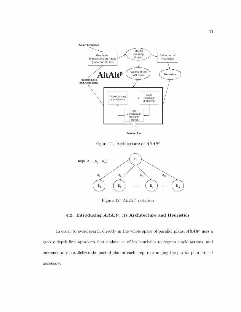
60
Action Templates
Problem Spec (Init, Goal state)
Solution Plan
Graphplan Plan Extension Phase
(based on STAN)
Parallel Planning Graph
Extraction of Heuristics
Heuristics Actions in the
Last Level
Node Expansion ( Fattening )
Node Ordering and Selection
Plan Compression
Algorithm ( PushUp )
AltAlt p
Figure 11. Architecture of AltAltp
. . . . . .
A =a 1 ,a 2 ,...,a p ,...a m
a 1 a 2 a p a m
S m S p S 2 S 1
S
Figure 12. AltAltp notation
4.2. Introducing AltAltp, its Architecture and Heuristics
In order to avoid search directly in the whole space of parallel plans, AltAltp uses a
greedy depth-first approach that makes use of its heuristics to regress single actions, and
incrementally parallelizes the partial plan at each step, rearranging the partial plan later if
necessary.

61
The high level architecture of AltAltp is shown in Figure 11. Notice that the heuris-
tic extraction phase of AltAltp is very similar to that of AltAlt, but with one important
modification. In contrast to AltAlt which uses a “serial” planning graph as the basis for
its heuristic (see Section 3.5), AltAltp uses the standard “parallel” planning graph. This
makes sense given that AltAltp is interested in parallel plans while AltAlt was aimed at
generating sequential plans. The regression state-space search engine for AltAltp is also
different from the search module in AltAlt. AltAltp augments the search engine of AltAlt
with (1) a fattening step and (2) a plan compression procedure (PushUp).
The general idea in AltAltp is to select a fringe action ap from among those actions A
used to regress a particular state S during any stage of the search (see Figure 12). Then, the
pivot branch given by the action ap is “fattened” by adding more actions from A, generating
a new state that is a consequence of regression over multiple parallel actions. The candidate
actions used for fattening the pivot branch must (a) come from the sibling branches of the
pivot branch, (b) be pairwise independent with all the other actions currently in the pivot
branch and (c) lead to better heuristic estimates. We use the standard definition of action
independence: two actions a1 and a2 are considered independent if the state S′ resulting
after regressing both actions simultaneously is the same as that obtained by applying a1
and a2 sequentially with any of their possible linearizations. A sufficient condition for this
is
((prec(a1) ∪ eff(a1)) ∩ (prec(a2) ∪ eff(a2))) = ∅

62
We now discuss in the next sections the details of the two main phases of AltAltp
used to generate parallel plans online, the fattening procedure and the plan compression
algorithm.
4.3. Selecting and Fattening a Search Branch in AltAltp
The first step in the AltAltp search engine is to select and parallelize a branch in
the search tree. Figure 13 shows the steps of the fattening procedure. The procedure first
identifies the set of regressable actions A for the current node S, and regresses each of them
computing the new children states. Next, the action leading to the child state with the
lowest heuristic cost among the new children is selected as the pivot action ap, and the
corresponding branch becomes the pivot branch.
The heuristic cost of the states is computed with the hadjsum2M heuristic 6 from
Chapter 3, based on a “parallel” planning graph. Based on the discussion on that section,
we compute the δ(p, q) values, which in turn depend on the level(p), level(q) and level(p, q)
in terms of the levels of a parallel planning graph rather than a serial planning graph. It is
easy to show that the level of a set of conditions on the parallel planning graph will be less
than or equal to the level on the serial planning graph. The length of the relaxed plan is
still computed in terms of number of actions.
The search algorithm used in AltAltp is similar to that used in AltAlt [Nguyen et al.,
2002; Sanchez et al., 2000], which has been already introduced in Chapter 3. But this time,
we slightly modify the evaluation function used to rank the nodes (f(S) = g(S)+w ∗h(S)).
In AltAltp, g(S) is the length of the current partial plan in terms of its number of steps,

63
parexpand(S)A ← get set of applicable actions for current state Sforall ai ∈ A
Si ← Regress(S,ai)CHILDREN(S) ← CHILDREN(S) + Si
Sp ← The state among Children(S) with minimumhadjsum2M valueap ← the action that regresses to Sp from S
/**Fattening processO ← ap forall g ∈ S ranked in the decreasing order of level(g)
Find an action ag ∈ A supporting g such that ag 6∈ O
and ai is pairwise independent with each action in O.If there are multiple such actions, pick the one that hasminimum hadjsum(Regress(S, O + ag)) among all ag ∈ A
If hadjsum2M (S, O + ai) < hadjsum2M (S, O)O ← O + ag
Spar ← Regress(S, O)CHILDREN(S) ← CHILDREN(S) + Spar
return CHILDRENEND;
Figure 13. Node expansion procedure
where each step may have multiple concurrent actions. h(S) is our estimated cost given by
the heuristic function based on a parallel planning graph, and w remains the same.
In case of a tie in selecting the pivot branch, i.e., more than one branch leads to a
state with the lowest heuristic cost, we break the tie by choosing the action that supports
subgoals that are harder to achieve. Here, the hardness of a literal l is measured in terms
of the level in the planning graph at which l first appears. The standard rationale for
this decision (c.f. [Kambhampati and Sanchez, 2000]) is that we want to fail faster by
considering the most difficult subgoals first. We have an additional justification in our case,
we also know that a subgoal with a higher level value requires more steps and actions for
its achievement because it appeared later into the planning graph. So, by supporting it

64
At(pack1,ASU) At(pack2,ASU) At(pack3,ASU)
At(pack4, Home)
S p S 1 S m
S
a p : Unload(pack1,airp1,ASU)
a 1 : Unload(pack1,airp2,ASU)
...
a m : Unload(pack4,airp2,Home)
H=21 H=22
H=23
Unload(pack2,airp1,ASU) Unload(pack2,airp2,ASU) Unload(pack3,airp1,ASU) Unload(pack3,airp2,ASU)
Unload(pack4,airp2,HOME)
H=21 Pivot
Possible Pairwise Independent Actions
Figure 14. After the regression of a state, we can identify the Pivot and the related set ofpairwise independent actions.
At(pack1,ASU) At(pack2,ASU) At(pack3,ASU)
At(pack4, Home)
S p S 1 S m
S
a p : Unload(pack1,airp1,ASU)
a 1 : Unload(pack1,airp2,ASU)
...
a m : Unload(pack4,airp2,Home)
H=21 H=22
H=23
Unload(pack1,airp1,ASU) Unload(pack2,airp1,ASU) Unload(pack2,airp2,ASU) Unload(pack3,airp1,ASU) Unload(pack3,airp2,ASU)
Unload(pack4,airp2,HOME)
H=21 Pivot
O
S par
a par : Unload(pack1,airp1,ASU) Unload(pack2,airp1,ASU) Unload(pack3,airp1,ASU)
H=19
Figure 15. Spar is the result of incrementally fattening the Pivot branch with the pairwiseindependent actions in O
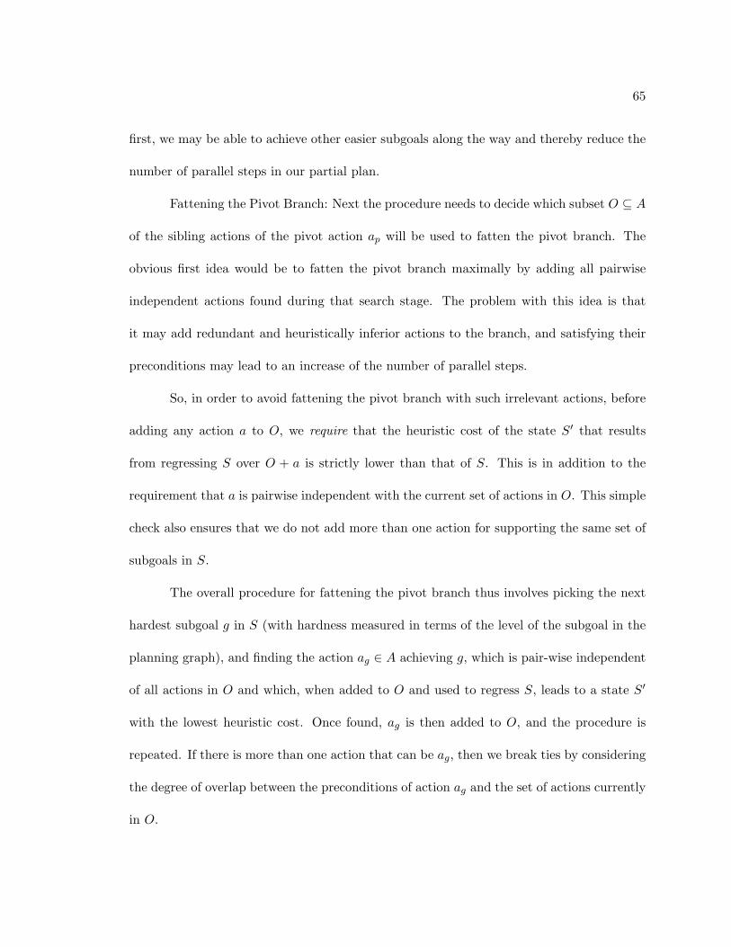
65
first, we may be able to achieve other easier subgoals along the way and thereby reduce the
number of parallel steps in our partial plan.
Fattening the Pivot Branch: Next the procedure needs to decide which subset O ⊆ A
of the sibling actions of the pivot action ap will be used to fatten the pivot branch. The
obvious first idea would be to fatten the pivot branch maximally by adding all pairwise
independent actions found during that search stage. The problem with this idea is that
it may add redundant and heuristically inferior actions to the branch, and satisfying their
preconditions may lead to an increase of the number of parallel steps.
So, in order to avoid fattening the pivot branch with such irrelevant actions, before
adding any action a to O, we require that the heuristic cost of the state S′ that results
from regressing S over O + a is strictly lower than that of S. This is in addition to the
requirement that a is pairwise independent with the current set of actions in O. This simple
check also ensures that we do not add more than one action for supporting the same set of
subgoals in S.
The overall procedure for fattening the pivot branch thus involves picking the next
hardest subgoal g in S (with hardness measured in terms of the level of the subgoal in the
planning graph), and finding the action ag ∈ A achieving g, which is pair-wise independent
of all actions in O and which, when added to O and used to regress S, leads to a state S′
with the lowest heuristic cost. Once found, ag is then added to O, and the procedure is
repeated. If there is more than one action that can be ag, then we break ties by considering
the degree of overlap between the preconditions of action ag and the set of actions currently
in O.
66
Definition 6. The degree of precondition overlap between an action a and the set of
actions chosen O is:
|prec(a) ∩ ∪o∈Oprec(o)|
The action a with higher degree of overlap is preferred as this will reduce the amount
of additional work we will need to do to establish its preconditions. Notice that because of
the fattening process, a search node may have multiple actions leading to it from its parent,
and multiple actions leading from it to each of its children.
Example 4.3
Figure 14 illustrates the use of this node expansion procedure for a problem from the
logistics domain [Bacchus, 2001]. In this example we have four packages pack1, pack2,
pack3 and pack4. Our goal is to place the first three of them at ASU and the remaining one
at home. There are two planes airp1 and airp2 to carry out the plans. The figure shows the
first level of the search after S has been regressed. It also shows the pivot action ap given
by unload(pack1,airp1,ASU), and a candidate set of pairwise independent actions with
respect to ap. Finally, we can see on Figure 15 the generation of the parallel branch. Notice
that each node can be seen as a partial regressed plan. As described in the paragraphs
above, only actions regressing to lower heuristics estimates are considered in apar to fatten
the pivot branch. Furthermore, we can also see that we have preferred actions using the
plane airp1, since they a higher degree of overlap with the pivot action ap.

67
pushUP(S)As ← get actions leading to Sforall a ∈ As
x ← 0Sx ← get parent node of S
/** Getting highest ancestor for each actionLoop
Ax ← get actions leading to Sx
If (parallel(a,Ax))x ← x + 1Sx ← get parent node of Sx−1
Else
aj ← get action conflicting with a from Ax
If (Secondary Optimizations)Remove a and aj from branchInclude anew if necessary
Else
Ax−1 ← Ax−1 + a
As ← As − a
breakEnd Loop
/**Adjusting the partial planSx ← get highest ancestor x in historycreateNewBranchFrom(Sx)while x > 0
Snew ← regress Sx with Ax−1
Sx ← Snew
x ← x− 1END;
Figure 16. PushUp procedure

68
At(pack1,ASU) At(pack2,ASU) At(pack3,ASU)
At(pack4, Home)
S p S 1 S m
S
Unload(pack1,airp1,ASU)
Unload(pack1,airp2,ASU)
...
Unload(pack4,airp2,Home)
H=21 H=21 H=22
H=23
S par
H=19
Unload(pack1,airp1,ASU) Unload(pack2,airp1,ASU) Unload(pack3,airp1,ASU)
S p ... S m S par
Unload(pack4,airp2,Home)
Unload(pack4,airp2,Home) fly(airp1,LocX,ASU)
fly(airp1,LocX,ASU)
H=18 Pivot
H=18
H=16
(a) Finding the highest ancestor node to which an action can bepushed up.
At(pack1,ASU) At(pack2,ASU) At(pack3,ASU)
At(pack4, Home)
S p S 1 S m
S
Unload(pack1,airp1,ASU)
Unload(pack1,airp2,ASU)
...
Unload(pack4,airp2,Home)
H=21 H=21 H=22
H=23
S par
H=19
Unload(pack1,airp1,ASU) Unload(pack2,airp1,ASU) Unload(pack3,airp1,ASU)
S p ... S m S par
Unload(pack4,airp2,Home)
fly(airp1,LocX,ASU) Unload(pack4,airp2,Home)
fly(airp1,LocX,ASU)
H=18 Pivot
H=18
H=16
S new
Unload(pack1,airp1,ASU) Unload(pack2,airp1,ASU) Unload(pack3,airp1,ASU)
Unload(pack4,airp2,HOME)
S new
fly(airp1,LocX,ASU)
H=16
(b) The PushUp procedure generates a new search branch.
Figure 17. Rearranging of the partial plan

69
4.4. Compressing Partial Plans to Improve Parallelism
The fattening procedure is greedy, since it insists that the state resulting after fatten-
ing have a strictly better heuristic value. While useful in avoiding the addition of irrelevant
actions to the plan, this procedure can also sometimes preclude actions that are ultimately
relevant but were discarded because the heuristic is not perfect. These actions may then
become part of the plan at later stages during search (i.e., earlier parts of the execution
of eventual solution plan; since we are searching in the space of plan suffixes). When this
happens, the parallel length of the solution plan is likely to be worsened, since more steps
that may be needed to support the preconditions of such actions would be forced to come at
even later stages of search (earlier parts of the plan). Had the action been allowed to come
into the partial plan earlier in the search (i.e., closer to the end of the eventual solution
plan), its preconditions could probably have been achieved in parallel to the other subgoals
in the plan, thus improving the number of steps.
In order to offset this negative effect of greediness, AltAltp re-arranges the partial
plan to promote such actions higher up the search branch (i.e., later parts of the execution
of the eventual solution plan). Specifically, before expanding a given node S, AltAltp checks
to see if any of the actions in As leading to S from its parent node (i.e., Figure 15 shows
that Apar leads to Spar) can be pushed up to higher levels in the search branch. This online
re-arrangement of the plan is done by the PushUp procedure, which is shown in Figure 16.
The PushUp procedure is called each time before a node gets expanded, and it will try to
compress the partial plan. For each of the actions a ∈ As we find the highest ancestor node
Sx of S in the search branch to which the action can be applied (i.e., it gives some literal in

70
Sx without deleting any other literals in Sx, and it is pairwise independent of all the actions
Ax currently leading out of Sx, in other words the condition parallel(a, Ax) is satisfied).
Once Sx is found, a is then removed from the set of actions As leading to S and introduced
into the set of actions leading out of Sx (to its child in the current search branch). Next, the
states in the search branch below Sx are adjusted to reflect this change. The adjustment
involves recomputing the regressions of all the search nodes below Sx. At first glance, this
might seem like a transformation of questionable utility since the preconditions of a (and
their regressions) just become part of the descendants of Sx, and this does not necessarily
reduce the length of the plan. We however expect a length reduction because actions
supporting the preconditions of a will get “pushed up” eventually during later expansions.
Rather than doctor the existing branch, in the current implementation, we just add
a new branch below Sx that reflects the changes made by the PushUp procedure.1 The new
branch then becomes the active search branch, and its leaf node is expanded next.
The PushUp procedure, as described above, is not expensive as it only affects the
current search branch, and the only operations involved are recomputing the regressions
in the branch. Of course, it is possible to be more aggressive in manipulating the search
branch. For example, after applying an action a to its ancestor Sx the set of literals in
the child state, say Snew changes, and thus additional actions may become relevant for
expanding Snew. In principle, we could re-expand Snew in light of the new information. We
decided not to go with the re-expansion option, as it typically does not seem to be worth
the cost. In the next section, we do compare our default version of PushUp procedure with
1Because of the way our data structures are set up, adding a new search branch turned out to be a morerobust option than manipulating the existing one.

71
a variant that re-expands all nodes in the search branch, and the results of those studies
support our decision to avoid re-expansion. Finally, although we introduced the PushUp
procedure as an add-on to the fattening step, it can also be used independent of the latter,
in which case the net effect would be an incremental parallelization of a sequential plan.
Example 4.4
In Figure 17(a), we have two actions leading to the node Spar (at depth two), these two
actions are Unload(pack4,airp2,Home) and fly(airp1,LocX,ASU). So, before expanding
Spar we check if any of the two actions leading to it can be pushed up. While the second
action is not pushable since it interacts with the actions in its ancestor node, the first
one is. We find the highest ancestor in the partial plan that interacts with our pushable
action. In our example the root node is such an ancestor. So, we insert our pushable action
Unload(pack4,airp2,Home) directly below the root node. We then re-adjust the state
Spar to Snew at depth 1, as shown in Figure 17(b) adding a new branch, and reflecting the
changes in the states below. Notice that we have not re-expanded the state Snew at depth 1,
we have only made the adjustments to the partial plan using the actions already presented
in the search trace.2
4.5. Results from Parallel Planning
We have implemented AltAltp on top of AltAlt. We have tested our implementation
on a suite of problems that were used in the 2000 and 2002 AIPS competition [Bacchus,
2Instead, the aggressive PushUp modification would expand Snew at depth 1, generating similar statesto those generated by the expansion of Spar at the same depth.

72
2001; Long and Fox, 2003], as well as other benchmark problems [McDermott, 2000]. Our
experiments are broadly divided into three sets, each aimed at comparing the performance
of AltAltp under different scenarios:
1. Comparing the performance of AltAltp to other planning systems capable of producing
parallel plans.
2. Comparing our incremental parallelization technique to AltAlt + Post-Processing.
3. Ablation studies to analyze the effect of the different parts of the AltAltp approach
on its overall performance.
Our experiments were all done on a Sun Blade-100 workstation, running SunOS 5.8
with 1GB RAM. Unless noted otherwise, AltAltp was run with the hadjsum2M heuristics
described in section 3.5 of this proposal, and with a parallel planning graph grown until the
first level where the top goals are present without being mutex. All times are in seconds.
4.5.1. Comparing AltAltp with Competing Approaches. In the first set of
experiments we have compared the performance of our planner with the results obtained by
running STAN [Long and Fox, 1999], Blackbox [Kautz and Selman, 1999], TP4 [Haslum and
Geffner, 2001], LPG [Gerevini and Serina, 2002] and SAPA [Do and Kambhampati, 2001].
Unless noted otherwise, every planner has been run with its default settings. Some of the
planners could not be run in some domains due to parsing problems or memory allocation
errors. In such cases, we just omit that planner from consideration for those particular
domains.

73
Logistics AIPS-00
0
10
20
30
40
50
60
70
80
90
1 4 7 10 13 16 19 22 25 28 31 34 37 40 43 46 49 52 55 58 61
Problems
Ste
ps
Altalt-p
STAN
TP4
Blackbox
LPG 2nd
(a)
Logistics AIPS-00
0
50
100
150
200
250
300
350
400
450
1 4 7 10 13 16 19 22 25 28 31 34 37 40 43 46 49 52 55 58 61
Problems
Tim
e
AltAlt-p
STAN
TP4
Blackbox
LPG 2nd
(b)
Figure 18. Performance on Logistics (AIPS-00)
74
4.5.1.1. Planners used in the Comparison Studies. As mentioned before, STAN is an
optimized version of the Graphplan algorithm that reasons with invariants and symmetries
to reduce the size of the search space. Blackbox is also based on the Graphplan algorithm
but it works by converting planning problems specified in STRIPS [Fikes and Nilsson, 1971]
notation into boolean satisfiability problems, solving them using a SAT solver (the version
we used defaults to SATZ).3 LPG [Gerevini and Serina, 2002] was judged the best perform-
ing planner at the 3rd International Planning Competition [Long and Fox, 2003], and it is a
planner based on planning graphs and local search inspired by the Walksat approach [Kautz
and Cohen, 1994]. LPG was run with its default heuristics and settings. Since LPG em-
ploys an iterative improvement algorithm, the quality of the plans produced by it can be
improved by running it for multiple iterations (thus increasing the running time). To make
the comparisons meaningful, we decided to run LPG for two iterations (n=2), since beyond
that, the running time of LPG was generally worse than that of AltAltp. Finally, we have
also chosen two metric temporal planners, which are able to represent parallel plans because
of their representation of time and durative actions. We consider TP4 [Haslum and Geffner,
2001], and the last planner in our list is SAPA [Do and Kambhampati, 2001]. SAPA is a
powerful domain-independent heuristic forward chaining planner for metric temporal do-
mains that employs distance-based heuristics [Kambhampati and Sanchez, 2000] to control
its search.
Logistics: The plots corresponding to the Logistics domain from [Bacchus, 2001] are shown
in Figure 18. For some of the most difficult problems AltAltp outputs lower quality solutions
3We have not chosen IPP [Koehler, 1999], which is also an optimized Graphplan planning system becauseresults in [Haslum and Geffner, 2001] show that it is already less efficient than STAN.

75
than the optimal approaches. However, only AltAltp and LPG are able to scale up to more
complex problems, and we can easily see that AltAltp provides better quality solutions than
LPG. AltAltp also seems to be more efficient than any of the other approaches. The LPG
solutions for problems 49 to 61 are obtained doing only one iteration, since LPG was not
able to complete the second iteration in a reasonable amount of time. This explains the low
time taken for LPG, but also the lower quality of its solutions.
Zeno-Travel: Only AltAltp, SAPA, and LPG are able to solve most of the problems in this
domain. AltAltp solves them very efficiently (Figure 19(b)) providing very good solution
quality (Figure 19(a)) compared to the temporal metric planners.
Summary: In summary, we note that AltAltp is second only to the Blackbox algorithm
in the problems that this optimal planner can solve in the Logistics domain. However, it
scales up along with LPG to bigger size problems, returning very good step-length quality
plans. In the ZenoTravel domain AltAltp is very efficient returning very good solutions.
TP4, the only other heuristic state-space search regression planner capable of producing
parallel plans is not able to scale up in most of the domains. SAPA, a heuristic search
progression planner, while competitive, is still outperformed by AltAltp in planning time
and solution quality.
4.5.2. Comparison to Post-Processing Approaches. As we mentioned earlier
(see Section 4.1), one way of producing parallel plans that has been studied previously in
the literature is to post-process sequential plans [Backstrom, 1998]. To compare online
parallelization to post-processing, we have implemented Backstrom’s “Minimal De-ordering
Algorithm” [Backstrom, 1998], and used it to post-process the sequential plans produced

76
ZenoTravel AIPS-02
0
5
10
15
20
25
30
35
40
1 2 3 4 5 6 7 8 9 10 11 12 13 14 15
Problems
Ste
ps
AltAlt-p
STAN
LPG 2nd
Sapa
(a)
ZenoTravel AIPS-02
0
500
1000
1500
2000
2500
3000
3500
4000
4500
5000
1 2 3 4 5 6 7 8 9 10 11 12 13 14 15
Problems
Tim
e AltAlt-p
STAN
LPG 2nd
Sapa
(b)
Figure 19. Performance on ZenoTravel (AIPS-02)

77
ZenoTravel AIPS-02
0
10
20
30
40
50
60
1 2 3 4 5 6 7 8 9 10 11 12 13 14 15
Problems
Ste
ps
AltAlt AltAlt-PostProc AltAlt-p
(a)
ZenoTravel AIPS-02
0
50
100
150
200
250
300
350
400
450
1 2 3 4 5 6 7 8 9 10 11 12 13 14 15
Problems
Tim
e
AltAlt AltAlt-PostProc AltAlt-p
(b)
Figure 20. AltAlt and Post-Processing vs. AltAltp (Zenotravel domain)

78
by AltAlt (running with its default heuristic hAdjSum2M using a serial planning graph). In
this section we will compare our online parallelization procedure to this offline method.
Figure 20 shows some experiments in the ZenoTravel domain [Long and Fox, 2003].
As expected, the original AltAlt has the longest plans since it allows only one action per
time step. The plot shows that post-processing techniques do help in reducing the makespan
of the plans generated by AltAlt. However, we also notice that AltAltp outputs plans with
better makespan than either AltAlt or AltAlt followed by post-processing. This shows that
online parallelization is a better approach than post-processing sequential plans. Moreover,
the plot in Figure 20(b) shows that the time taken by AltAltp is largely comparable to that
taken by the other two approaches. In fact, there is not much additional cost overhead in
our procedure.
4.5.3. Ablation Studies. This section attempts to analyze the impact of the dif-
ferent parts of AltAltp on its performance.
Utility of the PushUp Procedure: Figure 21 shows the effects of running AltAltp
with and without the PushUp procedure (but with the fattening procedure), as well as
running it with a more aggressive version of PushUp, which as described in Section 4.4,
re-expands all the nodes in the search branch, after an action has been pushed up. We
can see that running AltAltp with PushUp and fattening procedure is better than just the
latter. In Figure 21(b) we can see that although the PushUp procedure does not add much
overhead, the aggressive version of PushUp does get quite expensive. We also notice that
only around 20 problems are solved within time limits with aggressive PushUp. We can

79
Logistics AIPS-00
0
20
40
60
80
100
120
140
1 4 7 10 13 16 19 22 25 28 31 34 37 40 43 46 49 52 55 58 61
Problems
Ste
ps
AltAlt-p
AltAlt-p NoPush
AltAlt-p AGR
(a)
Logistics AIPS-00
0
100
200
300
400
500
600
1 4 7 10 13 16 19 22 25 28 31 34 37 40 43 46 49 52 55 58 61
Problems
Tim
e
AltAlt-p
AltAlt-p NoPush
AltAlt-p AGR
(b)
Figure 21. Analyzing the effect of the PushUp procedure on the Logistics domain

80
Logistics AIPS-00
0
10
20
30
40
50
60
70
80
1 4 7 10 13 16 19 22 25 28 31 34 37 40 43 46 49 52 55 58 61
Problems
Ste
ps Serial PG
Parallel PG
(a) Utility of using Parallel Planning Graphs
BlocksWorld AIPS-00
0
20
40
60
80
100
120
140
1 3 5 7 9 11 13 15 17 19 21 23 25 27 29 31 33 35
Problems
Tim
e
AltAlt-p
AltAlt
(b) Solving a Serial domain
Figure 22. Plots showing the utility of using parallel planning graphs in computing theheuristics, and characterizing the overhead incurred by AltAltp in serial domains.

81
conclude then that the PushUp procedure, used to offset the greediness of the algorithm,
achieves its purpose.
Utility of basing heuristics on Parallel Planning Graphs: We can see in Figure 22(a)
that using parallel planning graph as the basis for deriving heuristic estimates in AltAltp
is a winning idea. The serial planning graph overestimates the heuristic values in terms of
steps, producing somewhat longer parallel solutions. The fact that the version using serial
planning graph runs out of time in many problems also demonstrates that the running times
are also improved by the use of parallel planning graphs.
Comparison to AltAlt: One final concern would be how much of an extra computa-
tional hit is taken by the AltAltp algorithm in serial domains (e.g. Blocks World [Bacchus,
2001]). We expect it to be negligible since O = ∅. To confirm our intuitions, we ran AltAltp
on a set of problems from the sequential Blocks-world domain from [Bacchus, 2001]. We see
from the plot 22(b) that the time performance between AltAlt and AltAltp are equivalent
for almost all of the problems.4
4For a deeper analysis and more experiments see [Sanchez and Kambhampati, 2003a].

CHAPTER 5
Planning Graph Based Heuristics for Partial Satisfaction
(Over-subscription) Planning
Most planners handle goals of attainment, where the objective is to find a se-
quence of actions that transforms a given initial state I to some goal state G, where
G = g1 ∧ g2 ∧ ... ∧ gn is a conjunctive list of goal fluents. Plan success for these plan-
ning problems is measured in terms of whether or not all the conjuncts in G are achieved.
However, in many real world planning scenarios, the agent may only be able to partially sat-
isfy G, because of subgoal interactions, or lacking of resources and time. Effective handling
of partial satisfaction planning (PSP) problems poses several new challenges, including the
problem of designing efficient goal selection heuristics, and an added emphasis on the need
to differentiate between feasible and optimal plans based on new models for handling plan
quality (in terms of action costs and goal utilities). In this chapter, We provide a first
systematic analysis of PSP problems. We will start by distinguishing several classes of PSP
problems, but focus on one of the most general PSP problems, called PSP Net Benefit.
In this problem, each goal conjunct has a fixed utility attached to it, and each ground action

83
has a fixed execution cost associated with it. The objective is to find a plan with the best
“net benefit” (i.e., cumulative utility minus cumulative cost).
Despite the ubiquity of PSP problems, surprisingly little attention has been paid to
the development of effective approaches for solving them in the planning community. Earlier
work by the PYRRHUS system [Williamson and Hanks, 1994] allows for partial satisfaction
in planning problems with goal utilities. However, unlike the PSP problems discussed in this
Dissertation, PYRRHUS requires all goals to be achieved; partial satisfaction is interpreted
by using a non-increasing utility function on each of the goals. Many NASA planning prob-
lems have been identified as partial satisfaction problems [Smith, 2003]. Some preliminary
work by Smith (2004) proposed a planner for over-subscribed planning problems, in which
an abstract planning problem (i.e., the orienteering graph) is built to select the subset of
goals and orderings to achieve them. Smith (2004) speculated that the heuristic distance
estimates derived from a planning graph data structure are not particularly suitable for
PSP problems given that they make the assumption that goals are independent, without
solving the problem of interactions among them.
In this chapter, We show that in fact although planning graph estimates for PSP
problems are not very accurate in the presence of complex goal interactions, they can
also be extended to overcome such problems. In particular, We extend the reachability
analysis provided by planning graphs to compute cost-sensitive heuristics augmented with
mutex analysis to overcome over-subscribed planning problems. Our approach named Al-
tWlt [Sanchez and Kambhampati, 2005], involves a sophisticated multiple goal set selection
process augmented with mutex analysis in order to solve complex PSP problems. The
goal set selection process considers multiple combinations of goals and assigns penalty costs

84
based on mutex analysis when interactions are found. Once a subset of goal conjuncts is
selected, they are solved by a regression search planner with cost-sensitive planning graph
heuristics.
The rest of this chapter is organized as follows. First, We start by describing a
spectrum of PSP problems, and focus on the PSP Net Benefit problem, where actions
have execution costs and goals have utilities. After that, We will review AltAltps [van den
Briel et al., 2004b; 2004a], our initial approach to PSP, which forms the basis for AltWlt,
emphasizing its goals set selection algorithm and cost-sensitive reachability heuristics. In the
next part of this chapter, We will introduce AltWlt, pointing out the limitations of AltAltps
with some clarifying examples, and the extensions to overcome them. After that, We will
present a set of complex PSP problems and an empirical study on them that compares the
effectiveness of AltWlt with respect to its predecessor, and another experimental PSP based
planners. Finally, We conclude this chapter with some discussion on the current state of the
art alternative approaches, including among these Sapaps [Do and Kambhampati, 2004],
another planning-graph based heuristic planner, and the optimal MDP and IP formulation
to PSP Net Benefit to assess the quality of the solutions returned by AltWlt.
5.1. Problem Definition and Complexity
The following notation will be used: F is a finite set of fluents and A is a finite set
of actions, where each action consists of a list of preconditions and a list of add and delete
effects. I ⊆ F is the set of fluents describing the initial state and G ⊆ F is the set of
goal conjuncts. Hence we define a planning problem as a tuple P = (F, A, I, G). Figure 23
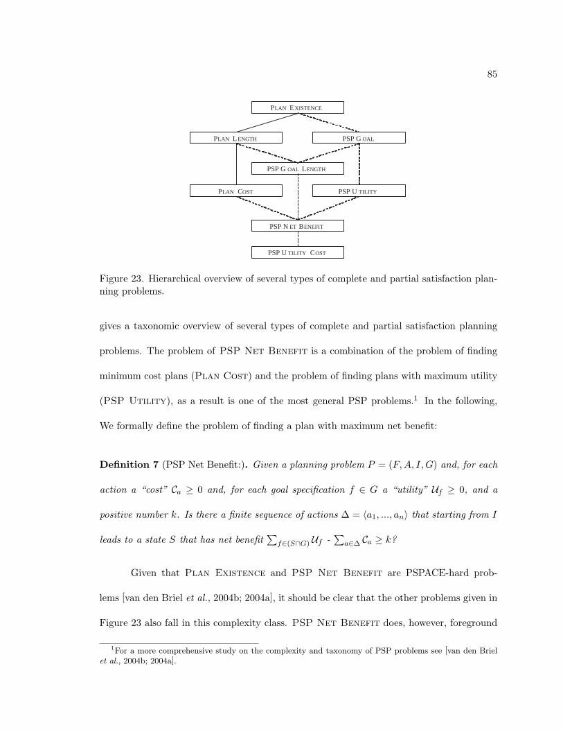
85
P LAN E XISTENCE
P LAN L ENGTH
PSP G OAL L ENGTH
PSP G OAL
P LAN C OST PSP U TILITY
PSP U TILITY C OST
PSP N ET B ENEFIT
Figure 23. Hierarchical overview of several types of complete and partial satisfaction plan-ning problems.
gives a taxonomic overview of several types of complete and partial satisfaction planning
problems. The problem of PSP Net Benefit is a combination of the problem of finding
minimum cost plans (Plan Cost) and the problem of finding plans with maximum utility
(PSP Utility), as a result is one of the most general PSP problems.1 In the following,
We formally define the problem of finding a plan with maximum net benefit:
Definition 7 (PSP Net Benefit:). Given a planning problem P = (F, A, I, G) and, for each
action a “cost” Ca ≥ 0 and, for each goal specification f ∈ G a “utility” Uf ≥ 0, and a
positive number k. Is there a finite sequence of actions ∆ = 〈a1, ..., an〉 that starting from I
leads to a state S that has net benefit∑
f∈(S∩G) Uf -∑
a∈∆ Ca ≥ k?
Given that Plan Existence and PSP Net Benefit are PSPACE-hard prob-
lems [van den Briel et al., 2004b; 2004a], it should be clear that the other problems given in
Figure 23 also fall in this complexity class. PSP Net Benefit does, however, foreground
1For a more comprehensive study on the complexity and taxonomy of PSP problems see [van den Brielet al., 2004b; 2004a].

86
Wp 0
Wp 2
Wp 1
C = 5
Wp 3
Wp 4
C = 10
C = 3
C = 15
C = 25
U = 30
U = 30
U = 30
U = 20
U = 20
Figure 24. Rover domain problem
the need to handle plan quality issues. To clarify the PSP Net Benefit problem, we
introduce the following example:
Example 5.1
Figure 24 illustrates again a small example from the rover domain [Long and Fox, 2003]
to motivate the need for partial satisfaction. 2 This time, a rover that has landed on
Mars needs to collect scientific data from some rock and soil samples. Some waypoints
have been identified on the surface. Each waypoint has scientific samples. For example,
waypoint3 has a rock sample, while waypoint4 has a soil sample. The rover needs to
travel to a corresponding waypoint to collect its samples. Each travel action has a cost
associated to it. For example, the cost of traveling from waypoint0 to waypoint1 is given
by Ctravel0,1= 10. In addition to the travelx,y actions, we have two more actions sample
and comm to collect and communicate the data respectively to the lander. To simplify our
problem, these actions have uniform costs independent of the locations where they take
2This time the notation of the problem is more descriptive to better understand it.

87
place. These costs are specified by Csampledata,x= 5 and Ccommdata,x,y
= 4. Each sample (or
subgoal) has a utility attached to it. We have a utility of Urock3= 30 for the rock sample
at waypoint3, and a utility Usoil4 = 20 for a soil sample at waypoint4. The goal of the
rover is to find a travel plan that achieves the best cost-utility tradeoff for collecting the
samples. In this example, the best plan is P = travel0,2 , samplerock2,2, commrock2,2,0,
travel2,1, samplerock1,1, commrock1,1,0, samplesoil1,1, commsoil1,1,0 which achieves the goals
rock2, rock1 and soil1, and ignores the rest of the samples at waypoint3 and waypoint4
giving the net benefit 45.
As mentioned before, current planning frameworks do not address the issue of partial
satisfaction of goals, because they strictly try to satisfy a conjunction of them. However,
this all-or-nothing success criterion does not seem to be very realistic. There are problems
where satisfying at least some of the goals is better than not satisfying any of them at
all. The problem is of course to choose the goals that will be satisfied with respect to an
optimization criteria. PSP problems could be solved optimally using Integer Programming
techniques [Haddawy and Hanks, 1993]. Unfortunately, current IP planning approaches do
not scale up well to bigger sized problems [Kautz and Walser, 1999; Vossen et al., 1999;
van den Briel et al., 2004b]. In the following section, we introduce AltAltps, our preliminary
heuristic approach to Partial Satisfaction (Over-subscription) Planning. First, We describe
how the cost information is propagated in a planning graph data structure, and then how
this information is used to select the set of goals upfront and guide the search of the planner.

88
5.2. Background: AltAltps Cost-based Heuristic Search and Goal Selection
In this section, We introduce AltAltps because it forms the basis for AltWlt, the
proposed algorithm that handles complex goal interactions. AltAltps is a heuristic regression
planner that can be seen as a variant of AltAlt [Sanchez et al., 2000; Nguyen et al., 2002]
equipped with cost sensitive heuristics. An obvious, if naive, way of solving the PSP Net
Benefit problem with such a planner is to consider all plans for the 2n subsets of an n-
goal problem, and see which of them will wind up leading to the plan with the highest net
benefit. Since this is infeasible, AltAltps uses a greedy approach to pick a goal subset up
front. The greediness of the approach is offset by considering the net benefit of covering
a goal not in isolation, but in the context of the potential (relaxed) plan for handling the
already selected goals. Once a subset of goal conjuncts is selected, AltAltps finds a plan
that achieves such subset using its regression search engine augmented with cost sensitive
heuristics. This description can be seen in the overall architecture of AltAltps in Figure 25.
Given that the quality of the plans for PSP problems depends on both the utility of
the goals achieved and the cost to achieve them, AltAltps needs heuristic guidance that is
sensitive to both action cost and goal utility. Because only the execution costs of the actions
and the achievement cost of propositions in the initial state (zero cost) are known, we need
to do cost-propagation from the initial state through actions to estimate the cost to achieve
other propositions, especially the top level goals. We can see in Figure 25 that AltAltps
is using the planning graph structure to compute this cost information. This information
over the planning graph is the basis for heuristic estimation in AltAltps, and is also used
to estimate the most beneficial subset of goals upfront and guide the search in the planner.

89
Action Templates
Problem Spec
(Init, Goal state)
Solution Plan
Graphplan Plan Extension Phase
(based on STAN)
+
Cost Propagation
Cost - sensitive Planning Graph
Extraction of Heuristics
Heuristics Actions in the
Last Level
Goal Set selection
Algorithm
Cost sensitive
Search
Action Templates
Problem Spec
(Init, Goal state)
Solution Plan
Graphplan Plan Extension Phase
(based on STAN)
+
Cost Propagation
Cost - sensitive Planning Graph
Extraction of Heuristics
Heuristics Actions in the
Last Level
Goal Set selection
Algorithm
Cost sensitive
Search
Figure 25. AltAltps architecture
The cost sensitive heuristics, as well as the goal set selection algorithm are described in
more detail in the next sections.
5.2.1. Propagating Cost as the Basis for Computing Heuristics. Follow-
ing [Do and Kambhampati, 2003], cost functions are used to capture the way cost of
achievement changes as the graph gets expanded. In the following, we briefly review the
procedure.
The purpose of the cost-propagation process is to build the cost functions C(f, lf )
and C(a, la) that estimate the cheapest cost to achieve fluent f at level lf of the planning
graph, and the cost to execute action a at level la. At the beginning (l = 0), let Sinit be
the initial state and Ca be the cost of action a then3: C(f, 0) = 0 if f ∈ Sinit, C(f, 0) =∞
otherwise; ∀a ∈ A : C(a, 0) =∞. The propagation rules are as follows:
3Ca and C(a, l) are different. If a = Travel0,1 then Ca is the travel cost and C(a, l) is the cost to achieve
preconditions of a at level l, which is the cost incurred to be at waypoint0 at l.

90
Figure 26. Cost function of at(waypoint1)
• C(f, l) = minC(a, l) + Ca) : f ∈ Eff(a)
• Max-prop: C(a, l) = maxC(f, l) : f ∈ Prec(a)
• Sum-prop: C(a, l) = ΣC(f, l) : f ∈ Prec(a)
The max-propagation rule will lead to an admissible heuristic, while the sum-
propagation rule does not. Assume that we want to reach waypoint1 in our rover example.
We can reach it directly from waypoint0 within a unit of time, or we can travel through
waypoint2 and reach it within two steps. Figure 26 shows the cost function for proposition
p1 = At(waypoint1), which indicates that the earliest level to achieve p1 is at l = 1 with the
lowest cost of 10 (route: waypoint0 → waypoint1). The lowest cost to achieve p1 reduces
to 8 at l = 2 (route: waypoint0 → waypoint2 → waypoint1) for the leveled planning graph.
There are many ways to terminate the cost-propagation process [Do and Kambham-
pati, 2003]: We can stop when all the goals are achievable, when the cost of all the goals
are stabilized (i.e. guaranteed not to decrease anymore), or lookahead several steps after

91
the goals are achieved. For classical planning, we can also stop propagating cost when the
graph levels-off [Nguyen et al., 2002].
5.2.2. Cost-sensitive Heuristics. Before describing the goal set selection process
of AltAltps, We introduce in this section cost-based heuristics that will help us to guide the
search of the planner once the goals have been selected. Notice that from the cost propa-
gation procedure described in the last section, we could easily derive the first heuristic for
our cost-based planning framework, computed under the assumption that the propositions
constituting a state are strictly independent. Such a heuristic is described as follows:
Sum Cost Heuristic 1. hsumC(S) =∑
p∈S C(p, l)4
The hsumC heuristic suffers from the same problems than the hsum heuristic intro-
duced by Bonet et al.,1997. It will tend to overestimate the cost of a set of propositions.
To make the heuristic admissible we could replace the sum function with the maximum
of the individual costs of the propositions composing the state. This leads us to our next
heuristic:
Max Cost Heuristic 2. hmaxC(S) = maxp∈S C(p, l)
This heuristic also directly resembles the hmax heuristic from [Bonet et al., 1997;
Nguyen et al., 2002], but in terms of cost. We could try to combine the differential power
of hsumC and hmaxC to get a more effective heuristic for a wider range of problems [Nguyen
et al., 2002].
4Where l = levels − off .

92
Combo Cost Heuristic 3. hcomboC(S) = hsumC(S) + hmaxC(S)
We could improve further the solution quality of our heuristics if we start taking
into account the positive interactions among subgoals while still ignoring the negative ones.
We could adapt the idea of the relaxed plan heuristic from [Hoffmann and Nebel, 2001;
Nguyen and Kambhampati, 2001; Nguyen et al., 2002] into our framework. So, AltAltps uses
variations of the relaxed plan extraction process guided by the cost-functions to estimate
heuristic values h(S) [Do and Kambhampati, 2003]. The basic idea is to compute the cost
of the relaxed plans in terms of the costs of the actions comprising them, and use such costs
as heuristic estimates. The general relaxed plan extraction process for AltAltps works as
follows:
1. Start from the goal set G containing the top level goals, remove a goal g from G and
select a lowest cost action ag (indicated by C(g, l)) to support g
2. Regress G over action ag, setting G = G ∪ Prec(ag)\Eff(ag)
The process above continues recursively until each proposition q ∈ G is also in the
initial state I. This regression accounts for the positive interactions in the state G given that
by subtracting the effects of ag, any other proposition that is co-achieved when g is being
supported is not counted in the cost computation. The relaxed plan extraction procedure
indirectly extracts a sequence of actions RP , which would have achieved the set G from the
initial state I if there were no negative interactions. The summation of the costs of the
actions ag ∈ RP can be used to estimate the cost to achieve all goals in G, in summary we
have:

93
Relax Cost Heuristic 4. hrelaxC(S) =∑
a∈RpCa
5.3. AltAltps Goal Set Selection Algorithm
The main idea of the goal set selection procedure in AltAltps is to incrementally
construct a new partial goal set G′ from the top level goals G such that the goals considered
for inclusion increase the final net benefit, using the goals utilities and costs of achievement.
The process is complicated by the fact that the net benefit offered by a goal g depends
on what other goals have already been selected. Specifically, while the utility of a goal g
remains constant, the expected cost of achieving it will depend upon the other selected goals
(and the actions that will anyway be needed to support them). To estimate the “residual
cost” of a goal g in the context of a set of already selected goals G′, we compute a relaxed
plan RP for supporting G′ + g, which is biased to (re)use the actions in the relaxed plan
R′P for supporting G′.
Figure 27 gives a description of the goal set selection algorithm. The first block
of instructions before the loop initializes our goal subset G′,5 and finds an initial relaxed
plan R∗P for it using the procedure extractRelaxedPlan(G′,∅). Notice that two arguments
are passed to the function. The first one is the current partial goal set from where the
relaxed plan will be computed. The second parameter is the current relaxed plan that
will be used as a guidance for computing the new relaxed plan. The idea is that we want
to bias the computation of the new relaxed plan to re-use the actions in the relaxed plan
from the previous iteration. Having found the initial subset G′ and its relaxed plan R∗P , we
5getBestBenefitialGoal(G) returns the subgoal with the best benefit, Ug − C(g, l) tradeoff

94
Procedure GoalSetSelection(G)
g ← getBestBenefitialGoal(G);
if(g = NULL)
return Failure;
G′ ← g; G← G \ g;
R∗
P ← extractRelaxedP lan(G′, ∅)
B∗
MAX ← getUtil(G′)− getCost(R∗
P );
BMAX ← B∗
MAX
while(BMAX > 0 ∧G 6= ∅)
for(g ∈ G \G′)
GP ← G′ ∪ g;
RP ← ExtractRelaxedP lan(GP , R∗
P )
Bg ← getUtil(GP )− getCost(RP );
if(Bg > B∗
MAX)
g∗ ← g; B∗
MAX ← Bg; R∗
g ← RP ;
else
BMAX ← Bg −B∗
MAX
end for
if(g∗ 6= NULL)
G′ ← G′ ∪ g∗; G ← G \ g∗; BMAX ←
B∗
MAX ;
end while
return G′;
End GoalSetSelection;
Figure 27. Goal set selection algorithm.

95
compute the current best net benefit B∗MAX by subtracting the costs of the actions in the
relaxed plan R∗P from the total utility of the goals in G′. B∗
MAX will work as a threshold
for our iterative procedure. In other words, we would continue adding subgoals g ∈ G to G′
only if the overall net benefit B∗MAX increases. We consider one subgoal at a time, always
computing the benefit added by the subgoal in terms of the cost of its relaxed plan RP and
goal utility Bg. We then pick the subgoal g that maximizes the net benefit, updating the
necessary values for the next iteration. This iterative procedure stops as soon as the net
benefit does not increase, or when there are no more subgoals to add, returning the new
goal subset G′.
In our running example, the original subgoals are g1 = soil1, g2 = rock1,
g3 = rock2, g4 = rock3, g5 = soil4, with final costs C(g, t) = 17, 17, 14, 34, 24 and
utilities vectors U = 20, 30, 30, 30, 20 respectively, where t = leveloff in the planning
graph. Following our algorithm, our starting goal g would be g3 because it returns the
biggest benefit (e.g. 30 - 14). Then, G′ is set to g3, and its initial relaxed plan R∗P is
computed. Assume that the initial relaxed plan found is R∗P = travel0,2, samplerock2
,
commrock2,2,0. We proceed to compute the best net benefit using R∗P , which in our exam-
ple would be B∗MAX = 30− (5 + 5 + 4) = 16. Having found our initial values, we continue
iterating on the remaining goals G = g1, g2, g4, g5. On the first iteration we compute
four different set of values, they are: (i) GP1= g3 ∪ g1, RP1
= travel2,1, samplesoil1 ,
commsoil1,2,0, travel0,2, samplerock2, commrock2,2,0, and Bgp1
= 24; (ii) GP2= g3 ∪ g2,
RP2= travel2,1, samplerock1
, commrock1,2,0, travel0,2, samplerock2, commrock2,2,0, and
Bgp2= 34; (iii) GP3
= g3 ∪ g4, RP3= travel0,3, samplerock3
, commrock3,2,0, travel0,2,
samplerock2, commrock2,2,0, and Bgp3
= 12, and (iv) GP4= g3 ∪ g5, RP4
= travel0,4,

96
samplesoil4 , commsoil4,2,0, travel0,2, samplerock2, commrock2,2,0 with Bgp4
= 12. Notice
then that our net benefit B∗MAX could be improved most if we consider goal g2. So, we
update G′ = g3 ∪ g2, R∗P = RP2
, and B∗MAX = 34. The procedure keeps iterating until
only g4 and g5 remain, which decrease the final net benefit. The procedure returns then
G′ = g1, g2, g3 as our goal set, which in fact it is the optimal goal set. In this example,
there is also a plan that achieves the five goals with a positive benefit, but it is not as good
as the plan that achieves the selected G′.
5.4. AltWlt: Extending AltAltps to Handle Complex Goal Scenarios
The advantage of AltAltps for solving PSP problems is that after committing to a
subset of goals, the overall problem is simplified to the planning problem of finding the
least cost plan to achieve the goal set selected, avoiding the exponential search on 2n goal
subsets. However, the goal set selection algorithm of AltAltps is greedy, and as a result it
is not immune from selecting a bad subset. The main problem with the algorithm is that
it does not consider goal interactions. Because of this limitation the algorithm may:
• return a wrong initial subgoal affecting the whole selection process, and
• select a set of subgoals that may not even be achievable due to negative interactions
among them.
The first problem corresponds to the selection of the initial subgoal g from where
the final goal set will be computed, which is one of the critical decisions of the algorithm.
Currently, the algorithm selects only the subgoal g with the highest positive net benefit.
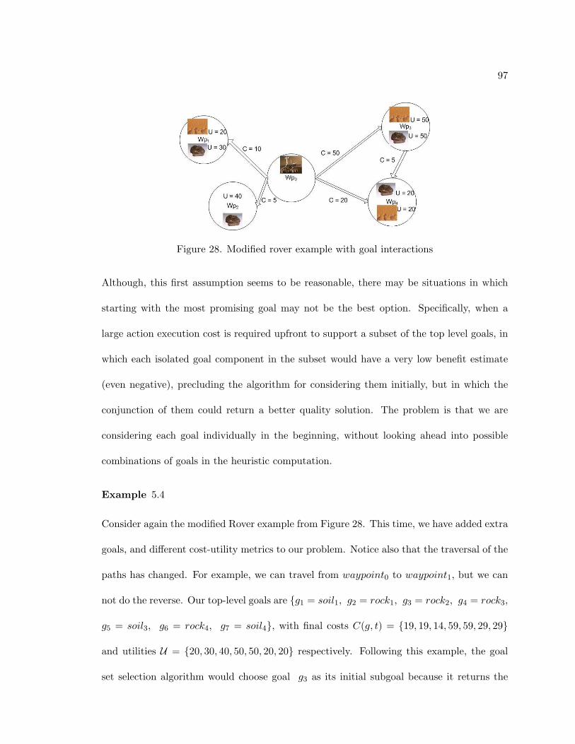
97
Figure 28. Modified rover example with goal interactions
Although, this first assumption seems to be reasonable, there may be situations in which
starting with the most promising goal may not be the best option. Specifically, when a
large action execution cost is required upfront to support a subset of the top level goals, in
which each isolated goal component in the subset would have a very low benefit estimate
(even negative), precluding the algorithm for considering them initially, but in which the
conjunction of them could return a better quality solution. The problem is that we are
considering each goal individually in the beginning, without looking ahead into possible
combinations of goals in the heuristic computation.
Example 5.4
Consider again the modified Rover example from Figure 28. This time, we have added extra
goals, and different cost-utility metrics to our problem. Notice also that the traversal of the
paths has changed. For example, we can travel from waypoint0 to waypoint1, but we can
not do the reverse. Our top-level goals are g1 = soil1, g2 = rock1, g3 = rock2, g4 = rock3,
g5 = soil3, g6 = rock4, g7 = soil4, with final costs C(g, t) = 19, 19, 14, 59, 59, 29, 29
and utilities U = 20, 30, 40, 50, 50, 20, 20 respectively. Following this example, the goal
set selection algorithm would choose goal g3 as its initial subgoal because it returns the

98
highest net benefit (e.g. 40 - 14). Notice this time that considering the most promising
subgoal is not the best option. Once the rover reaches waypoint2, it can not achieve any
other subgoal. In fact, there is a plan P for this problem with a bigger net benefit that
involves going to waypoint3, and then to waypoint4 collecting their samples. Our current
goal selection algorithm can not detect P because it ignores the samples on such waypoints
given that they do not look individually better than g3 (e.g. g4 has a benefit of 50 − 59).
This problem arises because the heuristic estimates derived from our planning graph cost
propagation phase assume that the goals are independent, in other words, they may not
provide enough information if we want to achieve several consecutive goals.
The second problem about negative interactions among goals is also exhibited in the
last example. We already mentioned that if we choose g3 we can not select any other goal.
However, our goal set selection algorithm would also select g1 and g2 given that the residual
cost returned by the relaxed plan heuristic is lower than the benefit added because it ignores
the negative interactions among goals. So, our final goal set would be G = g3, g2, g1, which
is not even achievable. Clearly, we need to identify such goal interactions and add some
cost metric when they exist.
We extended the goal selection algorithm in AltWlt to overcome these problems.
Specifically, this work considers multiple groups of subgoals, in which each subgoal from
the top level goal set is forced to be true in at least one of the groups, and also considers
adding penalty costs based on mutex analysis to account for complex interactions among
goals to overcome the limitations of the relaxed plan heuristic. Although these problems
could be solved independently, they can be easily combined and solved together. These
additions are discussed in the next sections.

99
Procedure MGS (G)
B∗
MAX ← −∞, G∗ ← ∅
for (gi ∈ G)
GLi ← nonStaticMutex(gi, G \ gi)
Rpi ← extractGreedyRelaxedP lan(gi, ∅)
G′
i ←
greedyGoalSetSelection(gi, GLi, Rpi)
NBi ← getUtil(G′
i)− getCost(Rpi)
if(NBi > B∗
MAX)
B∗
MAX ← NBi, G∗ ← G′
i
end for
return G∗;
End MGS ;
Figure 29. Multiple goal set selection algorithm
5.4.1. Goal Set Selection with Multiple Goal Groups. The general idea be-
hind the goal set selection with multiple groups procedure is to consider each goal gi from
the top level goal set G as a feasible starting goal, such that we can be able to find what
the benefit would be if such goal gi were to be part of our final goal set selected. The
idea is to consider more aggressively multiple combinations of goals in the selection process.
Although, we relax the assumption of having a positive net benefit for our starting goals,
the approach is still greedy. It modifies the relaxed plan extraction procedure to bias not
only towards those actions found in the relaxed plan of the previous iteration, but also
towards those facts that are reflected in the history of partial states of the previous relaxed
plan computation to account for more interactions. The algorithm will stop computing a
new goal set as soon as the benefit returned decreases. The new algorithm also uses mutex
analysis to avoid computing non-achievable goal groups. The output of the algorithm is the
goal group that maximizes our net benefit. A more detailed description of the algorithm is
shown in Figure 29, and is discussed below.

100
Given the set of top level goals G, the algorithm considers each goal gi ∈ G and finds
a corresponding goal subset G′i with positive net benefit. To get such subset, the algorithm
uses a modified greedy version of our original GoalSetSelection function (from Figure 27),
in which the goal gi has been set as the initial goal for G′i, and the initial relaxed plan Rpi
for supporting gi is passed to the function. Furthermore, the procedure only considers those
top-level goals left GLi ⊆ G which are not pair-wise static mutex with gi. The set GLi
is obtained using the procedure nonStaticMutex in the algorithm. By selecting only the
non-static mutex goals, we partially solve the problem of negative interactions, and reduce
the running time of the algorithm. However, we still need to do additional mutex analysis
to overcome complex goal interactions (e.g. dynamic mutexes); and we shall get back to
this below. At each iteration, the algorithm will output a selected goal set G′i given gi, and
a relaxed plan Rpi supporting it.
As mentioned in the beginning of this section, the modified
extractGreedyRelaxedP lan procedure takes into account the relaxed plan from the
previous iteration (e.g. Rp∗i ) as well as its partial execution history to compute the new
relaxed plan Rpi for the current subgoal gi. The idea is to adjust the aggregated cost of the
actions C(ai, l) supporting gi, to order them for inclusion in Rpi, when their preconditions
have been accomplished by the relaxed plan Rp∗i from the previous iteration. Remember
that C(ai, l) has been computed using our cost propagation rules, we decrease this cost
when Prec(ai) ∩∃ak∈Rp∗iEff(ak) 6= ∅ is satisfied. In other words, if our previous relaxed
plan Rp∗i supports already some of the preconditions of ai it better be the case that such
preconditions are not being over-counted in the aggregated cost of the action ai. This
greedy modification of our relaxed plan extraction procedure biases even more to our

101
previous relaxed plans, ordering differently the actions that will be used to support our
current subgoal gi. The idea is to try to adjust the heuristic positively to overcome the
independence assumption among subgoals.
For example, on Figure 28, assume that our previous relaxed plan Rp∗i has achieved
the subgoals at waypoint3, and we want to achieve subgoal gi = soil4. In order to collect
the sample, we need to be at waypoint4, the cheapest action in terms of its aggregated cost
that supports that condition is a = travel0,4 with cost of 20 which precludes gi for being
considered (no benefit added). However, notice that there is another action b = travel3,4
with original aggregated cost of 50 (due to its precondition), whose cost gets modified by
our new relaxed plan extraction procedure since its precondition (at waypoint3) is being
supported indirectly by our previous Rp∗i . By considering action b, the residual cost for
supporting soil4 lowers to 5, and as a result it can be considered for inclusion.
Finally, the algorithm will output the goal set G∗ that maximizes the net benefit
B∗MAX among all the different goal partitions G′
i. Following Example 2 from Figure 28, we
would consider 7 goal groups having the following partitions: g1 = soil1 & GL1 = g2,
g2 = rock1 & GL2 = g1, g3 = rock2 & GL3 = ∅, g4 = rock3 & GL4 = g5, g6, g7,
g5 = soil3 & GL5 = g4, g6, g7, g6 = rock4 & GL6 = g7, g7 = soil4 & GL7 = g6.
The final goal set returned by the algorithm in this example is G∗ = g4, g5, g6, g7, which
corresponds to the fourth partition G′4, with maximum benefit of 49. Running the original
algorithm (from Figure 27) in this example would select goal group G′3 = g3 with final
benefit of 26.
Even though our algorithm may look expensive since it is looking at different goal
combinations on multiple groups, it is still a greedy approximation of the full 2n combina-

102
tions of an optimal approach. The reduction comes from setting up the initial subgoals at
each goal group at each iteration. The worst case scenario of our algorithm would involve
to consider problems with no interactions and high goal utility values, in which the whole
set of remaining subgoals would need to be considered at each group. Given n top level
goals leading to n goal groups, the worst case running time scenario of our approach would
be in terms of n ∗∑n−1
i=1 i, which is much better than the factor 2n.
Notice that our multiple goal set selection process shares some similarities to the
Partition-k heuristic introduced in Section 3.5. The Partition-k heuristic tries to build sub-
sets of interacting goals, and then adds the amount of interactions found for each particular
subset built. The idea is to measure how costly a state is in terms of its subsets interactions.
Although, our MGS algorithm also takes into account subgoals interactions, it indirectly
behaves in an opposite direction to the Partition-k heuristic. The basic idea of MGS is to
keep adding subgoals to each goal subset if they increase the net benefit returned. Usually,
the subgoals added are those that are less costlier, which most of the times are also less
interacting with the current subset of goals. In other words, while MGS tries to measure
how beneficial a subset is, Partition-k considers how costly a subset could be.
5.4.2. Penalty Costs Through Mutex Analysis. Although the MGS algorithm
considers static mutexes, it still misses negative interactions among goals that could affect
the goal selection process. This is mainly due to the optimistic reachability analysis provided
by the planning graph. Consider again Example 5.4, and notice that goals g5 = soil3
and g7 = soil4 are not statically interfering, and they require a minimum of three steps
(actions) to become true in the planning graph (e.g. travel - sample - comm). However, at

103
level 3 of the planning graph these goals are mutex, implying that there are some negative
interactions among them. Having found such interactions, we could assign a penalty cost
PC to our residual cost estimate for ignoring them.
5.4.2.1. Penalty Costs Through Subgoal Interactions. A first approach for assigning
such a penalty cost PC , which we call NEGFM ,6 follows the work from [Nguyen et al.,
2002] considering the binary interaction degree δ among a pair of propositions. The idea is
that every time a new subgoal g gets considered for inclusion in our goal set G′, we compute
δ among g and every other subgoal g′ ∈ G′. At the end, we output the pair [g, g′] with
highest interaction degree δ if any. Recalling from Chapter 3, δ gets computed using the
following equation:
δ(p1, p2) = lev(p1 ∧ p2)−maxlev(p1), lev(p2) (5.1)
Where lev(S) corresponds to the set level heuristic that specifies the earliest level
in the planning graph in which the propositions in the set S appear and are not mutex to
each other [Nguyen et al., 2002]. Obviously, if not such level exists then lev(S) =∞, which
is the case for static mutex propositions.
The binary degree of interaction δ provided a clean way for assigning a penalty
cost to a pair of propositions in the context of heuristics based on number of actions,
given that δ was representing the number of extra steps (actions) required to make such
pair of propositions mutex free in the planning graph. Following our current example,
lev(g5 ∧ g7) = 5 (due to dummy actions), as a result δ(g5, g7) = 2 represents the cost for
6Negative Factor: Max

104
ignoring the interactions. However, in the context of our PSP problem, where actions have
real execution costs and propositions have costs of achievement attached to them, it is not
clear how to compute a penalty cost when negative interactions are found.
Having found the pair with highest δ(g, g′)g′∈G′ value, our first solution NEGFM
considers the maximum cost among both subgoals in the final level loff of the planning
graph as the penalty cost PC for ignoring such interaction. This is defined as:
PC(g, G′)NEGFM = max
(C(g, loff ), C(g′, loff ))
: g′ ∈ G′ ∧max(δ(g, g′))
(5.2)
NEGFM is greedy in the sense that it only considers the pair of interacting goals
with maximum δ value. It is also greedy in considering only the maximum cost among the
subgoals in the interacting pair as the minimum amount of extra cost needed to overcome
the interactions generated by the subgoal g being evaluated. Although NEGFM is easy
to compute, it is not very informative affecting the quality of the solutions returned. The
main reason for this is that we have already considered partially the cost of achieving g
when its relaxed plan is computed, and we are in some sense blindly over-counting the cost
if C(g, loff ) gets selected as the penalty PC . Despite these clear problems, NEGFM is able
to improve in problems with complex interactions over our original algorithm.
5.4.2.2. Penalty costs through action interactions. A better idea for computing the
negative interactions among subgoals is to consider the interactions among the actions
supporting such subgoals in our relaxed plans, and locate the possible reason for such
interactions to penalize them. Interactions could arise because our relaxed plan computation

105
Procedure NEGFAM (G,RpG, g′, ag′)
cost1 ← 0, cost2 ← 0
PC ← 0, maxCost← 0
for (gi ∈ G)
ai ← getSupportingAction(gi, RpG)
cost1 ←
competingNeedsCost(gi, ai, g′, ag′)
cost2 ← interferenceCost(gi, ai, g′, ag′)
maxCost← max(cost1, cost2)
if(maxCost > PC)
PC ← maxCost
end for
return PC ;
End NEGFAM ;
Figure 30. Interactions through actions
is greedy. It only considers the cheapest action7 to support a given subgoal g′, ignoring any
negative interactions of the subgoal. Therefore, the intuition behind this idea is to adjust the
residual cost returned by our relaxed plans, by assigning a penalty cost when interactions
among their goal supporting actions are found, in order to get better estimates. We called
this idea NEGFAM .8
NEGFAM is also greedy because it only considers the actions directly supporting
the subgoals in the relaxed plan, and it always keeps the interaction with maximum cost
as its penalty cost. In case that there is no supporting action for a given subgoal g′ (e.g. if
g′ ∈ I), the algorithm will take g′ itself for comparison. NEGFAM considers the following
types of action interaction based on [Weld, 1999]:
7With respect to C(a, l) + Ca8Negative Factor By Actions: Max

106
1. Competing Needs: Two actions a and b have preconditions that are statically mutually
exclusive, or at least one precondition of a is statically mutually exclusive with the
subgoal g′ given.
2. Interference: Two actions a and b, or one action a and a subgoal g′ are interfering if
the effect of a deletes b’s preconditions, or a deletes g′.
Notice that we are only considering pairs of static mutex propositions when we do
the action interaction analysis. The reason for this is that we just want to identify those
preconditions that are critically responsible for the actions interactions, and give a penalty
cost based on them. Once found a pair of static propositions, we have different ways of
penalizing them. We show the description of the NEGFAM technique on Figure 30. The
procedure gets the current selected goals G, the relaxed plan RpG supporting them, and the
subgoal g′ being evaluated and action ag′ supporting it. Then, it computes two different
costs, one based on the competing needs of actions, and the second one based on their
interference:
• For competing needs, we identify the proposition with maximum cost in the pair of
static preconditions of the actions, and we set PC to this cost. The idea is to identify
what the minimum cost would be in order to support two competing preconditions.
Given p1∧p2, where p1 ∈ Prec(ai) and p2 ∈ Prec(ag′), or p2 = g′ when ¬∃ag′, the cost
is cost1 = max(C(p1, leveloff),C(p2, leveloff)) if lev(p1 ∧ p2) = ∞. This penalty
gets computed using the procedure competingNeedsCost(gi, ai, g′, ag′) in Figure 30.
• In case of interference, our penalty cost PC is set to the cheapest alternate way (i.e.
action) for supporting a proposition being deleted. The idea is to identify what the

107
additional cost would be in order to restore a critical precondition, which needs to
be deleted to achieve another subgoal. Given p1 ∈ Prec(ai), and ¬p1 ∈ Eff(ag′) or
g′ = ¬p1, the cost is cost2 = minCx : ∀x s.t p1 ∈ Eff(x). This cost is computed
using the procedure InterferenceCost(gi, ai, g′, ag′).
Our algorithm then selects the cost that maximizes our return value PC given by the two
techniques mentioned above. Our PC is then added to the residual cost of subgoal g′.
Following our example 2 (Figure 28), we already mentioned that if we chose g3 =
rock2 we would also select g1 = soil1 and g2 = rock1 in our original algorithm, which is
not feasible. However, by taking into account the negative interactions among subgoals
with NEGFAM we would discard such unfeasible sets. For example, suppose that G =
g3 and RpG = travel0,2, samplerock2,2, commrock2,2,0, and the goal being considered
for inclusion is g′ = g1 with residual cost 19, corresponding to its relaxed plan Rpg′ =
travel0,1, samplesoil1,1, commrock1,1,0. Notice that the supporting actions for g3 and g1
are commrock2,2,0 and commsoil1,1,0 respectively. These actions have competing needs, one
action requires the rover to be at waypoint2 while the other one assumes the rover is at
waypoint1. The penalty cost PC given by NEGFAM for ignoring such interaction is 10,
which is the maximum cost among the static mutex preconditions. Adding this value to
our residual cost gives us a final cost of 29, which precludes the algorithm for considering
g1 (i.e. benefit = 20 - 29). Although NEGFAM is also greedy since it may over increase
the residual cost of a subgoal g′, it improves over our original algorithm and NEGFM ,
returning better quality solutions for problems with complex interactions (as will be shown
in our next section).

108
5.5. Empirical Evaluation
In the foregoing, We have described with illustrative examples, how complex inter-
actions may affect the goal set selection process of AltAltps. Our aim in this section is
to show that planning graph reachability heuristics augmented with mutex analysis still
provide efficient estimates for solving the PSP Net Benefit problem in the presence of
complex goal interactions.
Since there are no benchmark PSP problems, we used existing STRIPS planning
domains from the 2002 International Planning Competition [Long and Fox, 2003], and
modified them to support explicit declaration of goal utilities and action costs. 9 In par-
ticular, our experiments include the domains of DriverLog and Rover. For the DriverLog
domain, goal utilities ranged from 40 to 100, while the costs of the actions ranged from 3
to 70. Goal interactions were increased by considering bigger action execution costs, and
modified paths in the network that the planning agent has to traverse. The idea was to
place the most rewarding goals in the costlier paths of the network in order to increase
the complexity of finding the most beneficial subset of goals. For the Rover domain, utili-
ties ranged from 20 to 30, and action execution costs ranged from 4 to 45. In addition to
the modifications introduced in the DriverLog domain to increase the level of interactions
among goals, the Rover domain also allows for dead-ends, and loops in the network that
the rover has to traverse. The idea was to present more options for the planning agent to
fail. Consequently, it proved to be much more difficult to solve restricting even more the
9For a description of the domains and problems see Appendix A.

109
attainability of multiple goal sets. The design of this domain was inspired by the Rover
domain presented by Smith(2004), without considering resources in our domain description.
We compared our new approach AltWlt to its predecessor (AltAltps), and
Sapaps [van den Briel et al., 2004a]. Although Sapaps also uses planning graph heuristics
to rank their goals, it does not provide mutex analysis and its search algorithm is different.
We considered it pertinent to take into account both planners to see more clearly the impact
of the techniques introduced by this dissertation. See the next section for further discussion
on Sapaps [Do and Kambhampati, 2004].
We have also included in this section a run of OptiPlan [van den Briel et al., 2004a]
in the Rover domain, to demonstrate that our greedy approach is able to return high quality
plans. OptiPlan is a planner that builds on the work of solving planning problems through
IP [Vossen et al., 1999], which generates plans that are optimal for a given plan length.10
We did not compare to the approach presented by Smith(2004) because his approach was
not yet available by the time of this writing.11 All four planners were run on a P4 2.67Ghz
CPU machine with 1.0GB RAM.
Figure 31(a) shows our results in the DriverLog and Rover domains. We see that
AltWlt outperforms AltAltps and Sapaps in most of the problems, returning higher quality
solutions. In fact, it can be seen that AltWlt returns 13 times as much net benefit on average
than AltAltps in the DriverLog domain (i.e., a 1300% benefit increase). A similar scenario
occurs with Sapaps , where AltWlt returns 1.42 times as much more benefit on average (a
42% benefit increase). A similar situation occurs with the Rover domain in Figure 31 (b),
10For a more comprehensive description on OptiPlan see [van den Briel et al., 2004a].11Smith’s approach takes as input a non-standard PDDL language, without the explicit representation of
the operators descriptions.

110
in which AltWlt returns 10 and 12 times as much more benefit on average than AltAltps
and Sapaps respectively. This corresponds to a 1000% and 1200% benefit increase over
them. Although OptiPlan should in theory return optimal solutions for a given length, it
is not able to scale up, reporting only upper bounds on most of its solutions. Furthermore,
notice also in the plots that the total running time taken by AltWlt incurs a very little
additional overhead over AltAltps, and it is completely negligible in comparison to Sapaps
or OptiPlan.
Looking at the run times, it could appear at first glance that the set of problems
are relatively easy to solve given the total accumulated time of AltAltps. However, remem-
ber that for many classes of PSP problems, a trivially feasible, but decidedly non-optimal
solution would be the “null” plan, and AltAltps is in fact returning faster but much lower
quality solutions. We can see that the techniques introduced in AltWlt are helping the
approach to select better goal sets by accounting for interactions. This is not happening in
AltAltps, where the goal sets returned are very small and easier to solve.
We also tested the performance of AltWlt in problems with less interactions. Specif-
ically, we solved the suite of random problems from [van den Briel et al., 2004a], including
the ZenoTravel and Satellite planning domains [Long and Fox, 2003]. Although the gains
there were less impressive, AltWlt was able to produce in general better quality solutions
than the other approaches, returning bigger total net benefits.

111
(a) Cost-based Driverlog domain
(b) Cost-based Rover domain
Figure 31. Plots showing the total time and net benefit obtained by different PSP ap-proaches

CHAPTER 6
Related Work
As discussed in previous chapters, the advancement in planning is mainly due to the
extraction of heuristics from the problem representation. Heuristic state-space planning is
one of the most successful plan synthesis approaches. In consequence, most effective and
current planning systems are based on a combination of state-space search and planning
graph related heuristics. One main difference of our approach with respect to anyone else is
that our heuristic framework encodes positive as well as negative interactions among sub-
goals, improving the quality of our solutions. We will discuss in this Chapter the connections
of our work to alternative approaches, and state-of-the-art plan synthesis algorithms.
In the first section, we will discuss and survey related state-space planning algo-
rithms, emphasizing the main differences with respect to our approach, and possible venues
for improving our work. Then, we will explore work on parallel planning, highlighting the
limitations of competing approaches with respect to AltAltp. Finally, we will conclude
this Chapter by providing a background on over-subscription planning, and alternative
approaches to PSP Net Benefit.

113
6.1. Heuristic State-space Search and Disjunctive Planning
As we have already discussed in chapter 3, AltAlt has obvious rich connections
to the existing work on Graphplan [Blum and Furst, 1997; Long and Fox, 1999] and
regression state-space search planners [Bonet et al., 1997; Bonet and Geffner, 1999;
McDermott, 1999]. The closest planning algorithm to our approach is HSP-r [Bonet and
Geffner, 1999]. As mentioned before, HSP-r is a regression planner that mostly uses the
hadd heuristic to rank its search states. One of the main problems with such a heuristic
is that it assumes goal independence, thrashing badly in problems with high number of
interactions. Our approach however is able to extend on such ideas by considering positive
as well as negative interactions using relaxed plans and penalty costs. Moreover, the idea of
using the planning graph to select action instances and focus the regression search improves
our approach even further over HSP-r. This idea is similar to the RIFO [Koehler, 1999] and
helpful actions [Hoffmann and Nebel, 2001] techniques, that use relevance analysis to focus
progression search.
Although AltAlt has proven to be efficient and effective in a wide spectrum of plan-
ning problems, it lacks behind current state-of-the-art planning systems. Most successful
planning systems are currently based on some sort of forward state-space algorithm en-
hanced with different planning graph heuristic relaxations, as corroborated by the most
recent international planning competitions [Long and Fox, 2003; Hoffmann and Edelkamp,
2005]. Although progression search tends to have a bigger branching factor than regression
search, the states produced by progression search are complete and consistent, which in
turn results in more accurate heuristic estimates. Moreover, the relevance analysis used by

114
progression search algorithms helps them to reduce their branching factor improving their
overall efficiency.
One of such planning systems is FF [Hoffmann and Nebel, 2001]. FF’s base heuristic
can be seen as a graphplan relaxation. During its forward search, it computes from scratch
a relaxed plan for each state visited. Its relaxed plan heuristic takes into account positive
interactions among subgoals, and in that sense is similar to the hAdjSum2M heuristic of
AltAlt. However, negative interactions are still ignored. FF search strategy is a type of
enforced hill-climbing, combining local search and systematic search. The planner uses the
helpful actions technique from its relaxed plans to cut out search branches. In that sense,
it is similar to AltAlt using the PACTION procedure directly from the planning graph.
LPG [Gerevini and Serina, 2002] has been another very successful planning system
that also uses subgraphs from the planning graph data structure to guide its search. The
operators for moving from one search state into another are based on modifications to the
subgraphs. In that sense, its heuristics differ from the distance-based estimations discussed
in this Dissertation given that they weight how costly is to repair the inconsistencies found
in a particular subgraph.
As discussed in [Nguyen and Kambhampati, 2000; Nguyen et al., 2002], there are also
several rich connections between our strategies for deriving the heuristics from the planning
graphs, and recent advances in heuristic search, such as pattern databases [Culberson and
Schaeffer, 1998], capturing subproblem interactions [Korf and Taylor, 1996; Korf, 1997], and
greedy regression tables [Refanidis and Vlahavas, 2001] by the GRT planning system. It is
worth to mention that the GRT planning system implements a progression search algorithm,
but it only computes its heuristic once backwards from the top level goals as a preprocessing
115
step. In order to construct the heuristic backwards, the actions of the problem have to be
inverted, enhancing the top level goal set with the missing propositions to obtain better
estimates for its tables, and discarding objects that are not relevant. Notice that in our case
a similar idea could be tried during the regression search of AltAlt. Remember that the
states resulting from regression search constitute partial assignments (i.e, they represent a
set of states due to the missing propositions). In consequence, we could try to enhance (or
complete) our regressed states to also improve our heuristics during search.
Finally, one of the most recent and successful planners is Fast Downward [Helmert
and Richter, 2004; Helmert, 2004]. Motivated by the fact that progression planners tend
to suffer in domains with deadends or frequent plateau regions (since most of them ignore
negative interactions among subgoals), the Fast Downward algorithm introduced multi-
value state variables as a natural way of computing and compactly representing subgoals
and their interactions. Fast Downward uses hierarchical decompositions of planning tasks
based on causal graphs for computing its heuristic function. The main idea of the heuristic
is to split the planning task, and combine the lengths of the solutions of the parts to form
a distance heuristic for the overall task. The heuristic estimates the cost of changing the
values of the state variables in the subtasks. In that sense, it is similar to LPG, which tries
to repair locally the inconsistencies of its subgraphs.
Although AltAlt lacks behind the current state-of-the-art planning systems, it still
remains as one of the best regression state-space search planners up to date. Moreover,
some of the new techniques employed by progression planners could be extended to improve
the two phases of our approach, the heuristics and the search process. For example, the
multi-value state variable representation of Fast Downward could be adapted to improve

116
the planning graph expansion phase of AltAlt. Moreover, the use of helpful actions and
consistency enforcement techniques, such as those described in [Hoffmann and Nebel, 2001;
Gerevini and Schubert, 1998; Fox and Long, 1998; Rintanen, 2000], could be tried to further
improve the backward search algorithm of AltAlt.
6.2. State-space Parallel Planning and Heuristics
The idea of partial exploration of parallelizable sets of actions is not new [Kabanza,
1997; Godefroid and Kabanza, 1991; Do and Kambhampati, 2001]. It has been studied in
the area of concurrent and reactive planning, where one of the main goals is to approximate
optimal parallelism. However, most of the research there has been focused on forward
chaining planners [Kabanza, 1997], where the state of the world is completely known. It
has been implied that backward-search methods are not suitable for this kind of analysis
[Godefroid and Kabanza, 1991] because the search nodes correspond to partial states. We
have shown in Chapter 4 that backward-search methods can also be used to approximate
parallel plans in the context of classical planning.
Optimization of plans according to different criteria (e.g. execution time, quality,
etc) has also been done as a post-processing step. The post-processing computation of a
given plan to maximize its parallelism has been discussed by Backstrom(1998). Reordering
and de-ordering techniques are used to maximize the parallelism of the plan. In de-ordering
techniques ordering relations can only be removed, not added. In reordering, arbitrary
modifications to the plan are allowed. In the general case this problem is NP-Hard and
it is difficult to approximate [Backstrom, 1998]. Furthermore, as discussed in Section 4.1,

117
post-processing techniques are just concerned with modifying the order between the existing
actions of a given plan. Our approach not only considers modifying such orderings but also
inserting new actions online which can minimize the possible number of parallel steps of
the problem.
We have already discussed Graphplan based planners [Long and Fox, 1999; Kautz
and Selman, 1999], which return optimal plans based on the number of time steps. As
mentioned in Chapter 4, Graphplan uses IDA* to include the greatest number of parallel
actions at each time step of the search. However, this iterative procedure is very time
consuming and it does not provide any guarantee on the number of actions in its final plans.
There have been a few attempts to minimize the number of actions in these planners [Huang
et al., 1999] by using some domain control knowledge based on the generation of rules for
each specific planning domain. The Graphplan algorithm tries to maximize its parallelism
by satisfying most of the subgoals at each time step, if the search fails then it backtracks
and reduces the set of parallel actions being considered one level before. AltAltp does the
opposite, it tries to guess initial parallel nodes given the heuristics, and iteratively adds
more actions to these nodes as possible with the PushUp procedure later during search.
More recently, there has been some work on generalizing forward state-space search
to handle action concurrency in metric temporal domains. Of particular relevance to this
work are the temporal TLPlan [Bacchus and Ady, 2001] and SAPA [Do and Kambhampati,
2001] planners. Both of these planners are designed specifically for handling metric temporal
domains, and use similar search strategies. The main difference between them being that
Temporal TLPlan depends on hand-coded search control knowledge to guide its search,
while SAPA (like AltAltp) uses heuristics derived from (temporal) planning graphs. As

118
such, both these planners can be co-opted to produce parallel plans in classical domains.
Both these planners do a forward chaining search, and like AltAltp, both of them achieve
concurrency incrementally, without projecting sets of actions, in the following way. Normal
forward search planners start with the initial state S0, corresponding to time t0, consider
all actions that apply to S0, and choose one, say a1 apply it to S0, getting S1. They
simultaneously progress the “system clock” from t0 to t1. In order to allow for concurrency,
the planners by Bacchus and Ady, and Do and Kambhampati essentially decouple the
“action application” and “clock progression.” At every point in the search, there is a non-
deterministic choice - between progressing the clock, or applying (additional) actions at
the current time point. From the point of view of these planners, AltAltp can be seen as
providing heuristic guidance for this non-deterministic choice (modulo the difference that
AltAltp does regression search). The results of empirical comparisons between AltAltp and
SAPA, which show that AltAltp outperforms SAPA, suggest that the heuristic strategies
employed in AltAltp including the incremental fattening, and the pushup procedure, can
be gainfully adapted to these planners to increase the concurrency in the solution plans.
Finally, HSP*, and TP4, its extension to temporal domains, are both heuristic state-space
search planners using regression that are capable of producing parallel plans [Haslum and
Geffner, 2000]. TP4 can be seen as the regression version of the approach used in SAPA
and temporal TLPlan. Our experiments however demonstrate that neither of these planners
scales well in comparison to AltAltp.
The PushUp procedure can be seen as a plan compression procedure. As such, it is
similar to other plan compression procedures such as “double-back optimization” [Crawford,
1996]. One difference is that double-back is used in the context of a local search, while

119
PushUp is used in the context of a systematic search. Double-back could be also applied to
any finished plan or schedule, but as any other post-processing approach its outcome would
depend highly on the plan given as input. We can conclude that our approach AltAltp
remains as the state-of-the-art in the generation of parallel plans through state-space search.
6.3. Heuristic Approaches to Over-subscription Planning
As mentioned in Chapter 5, there has been very little work on PSP in planning. One
possible exception is the PYRRHUS planning system [Williamson and Hanks, 1994] which
considers an interesting variant of the partial satisfaction planning problem. In PYRRHUS,
the quality of the plans is measured by the utilities of the goals and the amount of resource
consumed. Utilities of goals decrease if they are achieved later than the goals’ deadlines.
Unlike the PSP problem discussed in this Thesis, all the logical goals still need to be achieved
by PYRRHUS for the plan to be valid. It would be interesting to extend the PSP model
to consider degree of satisfaction of individual goals.
More recently, Smith (2003) motivated oversubscription problems in terms of their
applicability to the NASA planning problems. Smith (2004) also proposed a planner for
oversubscription in which the solution of the abstracted planning problem is used to select
the subset of goals and the orders to achieve them. The abstract planning problem is built
by propagating the cost on the planning graph and constructing the orienteering problem.
The goals and their orderings are then used to guide a POCL planner. In this sense, this
approach is similar to AltAltps; however, the orienteering problem needs to be constructed
using domain-knowledge for different planning domains. Smith (2004) also speculated that

120
planning-graph based heuristics are not particularly suitable for PSP problems where goals
are highly interacting. His main argument is that heuristic estimates derived from planning
graphs implicitly make the assumption that goals are independent. However, as shown in
this Dissertation, reachability estimates can be improved using the mutex information also
contained in planning graphs, allowing us to solve problems with complex goal interactions.
Probably the most obvious way to optimally solve the PSP Net Benefit problem
is by modeling it as a fully-observable Markov Decision Process (MDP) [Hoey et al., 1999]
with a finite set of states. MDPs naturally permit action cost and goal utilities, but we
found in our studies that an MDP based approach for the PSP Net Benefit problem
appears to be impractical, even the very small problems generate too many states. To
prove our assumption, we modeled a set of test problems as MDPs and solved them using
SPUDD [Hoey et al., 1999].1 SPUDD is an MDP solver that uses value iteration on alge-
braic decision diagrams, which provides an efficient representation of the planning problem.
Unfortunately, SPUDD was not able to scale up, solving only the smallest problems.2
Remember also that PSP problems could be solved optimally using Integer Pro-
gramming techniques [Haddawy and Hanks, 1993]. An approach included in our evaluation
section is OptiPlan. OptiPlan is a planning system that provides an extension to the state
change programming (IP) model by Vossen et al.(1999). The main extension in OptiPlan
is the use of Graphplan [Blum and Furst, 1997] to eliminate many unnecessary variables.
Unfortunately, the current version of OptiPlan does not scale up well to bigger sized prob-
lems.
1We thank Will Cushing and Menkes van den Briel who first suggested the MDP modeling idea.2Details on the MDP model and results can be found in [van den Briel et al., 2005].

121
The only other heuristic state-space based approach to PSP is Sapaps [Do and
Kambhampati, 2004; van den Briel et al., 2004a]. Unlike to AltWlt, Sapaps does not select
a subset of the goals up front, but uses an anytime A* heuristic search framework in which
goals are treated as “soft constraints” to select them during planning. Any executable plan
is considered a potential solution, with the quality of the plan measured in terms of its net
benefit. Sapaps is a forward state space planner, which does not include mutex analysis in
its search framework.
Over-subscription issues have received relatively more attention in the scheduling
community. Earlier work in over-subscription scheduling used greedy approaches, in which
tasks of higher priorities are scheduled first [Kramer and Giuliano, 1997; Potter and Gasch,
1998]. The approach used by AltWlt is more sophisticated in that it considers the residual
cost of a subgoal in the context of an existing partial plan for achieving other selected goals,
taking into account complex interactions among the goals. More recent efforts have used
stochastic greedy search algorithms on constraint-based intervals [Frank et al., 2001], genetic
algorithms [Globus et al., 2003], and iterative repairing technique [Kramer and Smith, 2003]
to solve this problem more effectively.

CHAPTER 7
Concluding Remarks
The current work is motivated by the need of domain independent heuristic estima-
tors by plan synthesis algorithms. Heuristic functions that can be extracted automatically
from the problem representation, and that can be used across different planning problems
and domains. Particularly, we have shown in this Dissertation, that state-space planning
can be more efficient and effective in solving more complex problems when enhanced with
heuristic functions. A novel heuristic framework was developed based on the reachabil-
ity information encoded in planning graphs. It was shown that distance-based heuristics
extracted from planning graphs are powerful approximations for a variety of planning prob-
lems.
More specifically, techniques for controlling the cost of computing the heuristics and
reducing the branching factor of the search were introduced. Planning graph heuristics
were also developed for parallel state-space planning, where an online plan compression
algorithm was designed to improve even further the quality of the solutions returned by
the system. The empirical evaluation showed that the greedy approach was an attractive
tradeoff between quality and efficiency in the generation of parallel plans.

123
The portability of the heuristic estimates was again demonstrated when we adjusted
state-space planning to account for over-subscription planning problems. A greedy algo-
rithm was developed that is able to select a subset of the top-level goals upfront using
planning graph estimates. It was also shown, that the mutex analysis from the planning
graph is a rich source of information for improving even further the heuristics, addressing
more complex planning problems.
Finally, extensive empirical analysis on each different application of state-space plan-
ning was presented at each chapter, highlighting the heuristics used by the algorithms.
Related work on heuristic planning was also discussed at the end of the dissertation.
7.1. Future Work
The solutions presented by this work are based on state-space planning, more
specifically regression planning. Although, regression state-space planning considers rel-
evance of actions to reduce the branching factor of the search, this one can still be
quite large, producing many inconsistent states. A better alternative would be to con-
sider lifted planning representations, in which states are partially instantiated. One of
the main advantages of lifting is the reduction of the planner’s search space by delaying
the introduction of ground atoms into the plan, thus avoiding the large branching fac-
tor of planning problems [Yang and Chan, 1994; Younes and Simmons, 2002]. In conse-
quence, lifting avoids the problem of excessive memory usage [Ginsberg and Parkes, 2000;
Parkes, 1999] by pruning the search space. However, there does not yet exist a convincing
approach for planning with lifted actions. This is mainly due to the lack of heuristics for

124
partially instantiated states, and the overhead for maintaining consistency on the bindings
of the lifted operators. Furthermore, the indexing and caching schemas that are essen-
tial to the speed of ground actions [Parkes, 1999] may not be directly applicable to lifted
representations.
A lifted state would have some variables and certain domains of values over them. In
fact, a partially instantiated state would represent a set of states, each one would correspond
to an assignment of the values to the free variables in the state. The challenge would be
to adjust the reachability information provided by planning graphs to cover most of the
variables in the state, without enumerating all different instantiations. One simple, but
naive idea would be to consider the minimum cost (e.g., level information) in the planning
graph among all different instantiations of a particular variable. However, as mentioned
before, this heuristic would be too costly to compute since we would need to enumerate all
possible combinations of values for each variable. A better tradeoff would be to consider
distance as well as cover information for each particular variable. In other words, issues like:
variables appearing more in a state, cardinality of the variables (i.e., size of their domains),
and reachability information may be critical to compute good heuristic estimates. Future
work will try to shed light on these issues, understanding that lifting could be of great help
for those particular planning problems (e.g., probabilistic planning, temporal planning,
planning under uncertainty, etc) where the branching factor of the search is a real and
complicated problem.
As mentioned in Chapter 1, taking into account complex goal interactions to compute
admissible heuristics remains a challenging problem. Another future direction would be
to consider positive as well as negative goal interactions in the application of distance-

125
based heuristics in other critical planning frameworks, including among these temporal
planning and least commitment planning where negative interactions are mostly ignored.
The effectiveness of considering positive interactions by the relax plan heuristic has been
widely shown [Hoffmann and Nebel, 2001; Nguyen et al., 2002; Gerevini and Serina, 2002],
and we believe that there are problems in which negative interactions play a crucial role,
but, unfortunately, no planning system has addressed such issue at all. Planning graphs
provide a natural way of considering strong interactions, and we plan to further exploit
them, in other more complex planning frameworks.

REFERENCES
[Ai-Chang et al., 2004] M. Ai-Chang, J. Bresina, L. Charest, A. Chase, J. Cheng jung Hsu,
A. Jonsson, B. Kanefsky, P. Morris, K. Rajan, J. Yglesias, Brian G. Chafin, William C.
Dias, and Pierre F. Maldague. MAPGEN: Mixed-initiative planning and scheduling for
the mars exploration rover mission. IEEE Intelligent Systems, 19(1):8–12, January 2004.
[Bacchus and Ady, 2001] F. Bacchus and M. Ady. Planning with Resources and Concur-
rency: A Forward Chaining Approach. In Proceedings of IJCAI-01, pages 417–424, 2001.
[Bacchus, 2001] F. Bacchus. The AIPS’00 planning competition. AI Magazine, 22(3):47–56,
Fall 2001.
[Backstrom, 1998] C. Backstrom. Computational Aspects of Reordering Plans. Journal of
Artificial Intelligence Research, 9:99–137, 1998.
[Blum and Furst, 1997] A. Blum and M.L. Furst. Fast Planning Through Planning Graph
Analysis. Artificial Intelligence, 90:281–300, 1997.
[Blythe et al., 2003] J. Blythe, E. Deelman, Y. Gil, C. Kesselman, A. Agarwal, G. Mehta,
and K. Vahi. The role of planning in grid computing. In Proceedings of the 13th Inter-
national Conference on Automated Planning and Scheduling (ICAPS-03), June 2003.

127
[Bonet and Geffner, 1999] B. Bonet and H. Geffner. Planning as Heuristic Search: New
Results. In Proceedings of ECP-99, 1999.
[Bonet and Geffner, 2001] B. Bonet and H. Geffner. Heuristic Search Planner 2.0. AI
Magazine, 22(3):77–80, Fall 2001.
[Bonet et al., 1997] B. Bonet, G. Loerincs, and H. Geffner. A Robust and Fast Action
Selection Mechanism for Planning. In Proceedings of AAAI-97, pages 714–719. AAAI
Press, 1997.
[Bryce and Kambhampati, 2004] D. Bryce and S. Kambhampati. Heuristic guidance mea-
sures for conformant planning. In Proceedings of the 14th International Conference on
Automated Planning and Scheduling (ICAPS-04), June 2004.
[Bylander, 1994] T. Bylander. The computational complexity of propositional STRIPS
planning. Artificial Intelligence, 69(1–2):165–204, 1994.
[Chien et al., 2000] S. Chien, G.Rabideau, R. Knight, R. Sherwood, B. Engelhardt,
D. Mutz, T. Estlin, B. Smith, F. Fisher, T. Barrett, G. Stebbins, and D. Tran. As-
pen - automated planning and scheduling for space mission operations. 6th International
Symposium on Space Missions Operations, June 2000.
[Committee, 1998] AIPS-98 Planning Competition Committee. Pddl - the planning domain
definition language. Technical Report CVC TR-98-003/DCS TR-1165, Yale Center for
Computational Vision and Control, 1998.

128
[Crawford, 1996] J. Crawford. An Approach to Resource-constrained Project Scheduling.
In Proceedings of the 1996 Artificial Intelligence and Manufacturing Research Planning
Workshop. AAAI Press, 1996.
[Culberson and Schaeffer, 1998] J. Culberson and J. Schaeffer. Pattern databases. Compu-
tational Intelligence, 14(4), 1998.
[Dean and Wellman, 1991] T. Dean and M. Wellman. Planning and Control. Morgan Kauf-
mann, first edition, 1991.
[Do and Kambhampati, 2000] Minh B. Do and S. Kambhampati. Solving Planning Graph
by Compiling it into a CSP. In Proceedings of AIPS-00, pages 82–91, 2000.
[Do and Kambhampati, 2001] Minh B. Do and S. Kambhampati. SAPA: A Domain-
Independent Heuristic Metric Temporal Planner. In Proceedings of ECP-01, 2001.
[Do and Kambhampati, 2003] M. Do and S. Kambhampati. Sapa: a multi-objective metric
temporal planner. JAIR, 20:155–194, 2003.
[Do and Kambhampati, 2004] M. Do and S. Kambhampati. Partial satisfaction (over-
subscription) planning as heuristic search. In Proceedings of KBCS-04, 2004.
[Erol et al., 1995] K. Erol, D. Nau, and V. Subrahmanian. Complexity, decidability, and un-
decidability results for domain-independent planning. Artificial Intelligence, 76(1-2):75–
88, 1995.
[Fikes and Nilsson, 1971] R. Fikes and N. Nilsson. Strips: A new Approach to the Appli-
cation of Theorem Proving to Problem Solving. Artificial Intelligence, 2(3-4):189–208,
1971.

129
[Fox and Long, 1998] M. Fox and D. Long. Automatic inference of state invariants in TIM.
JAIR, 9, 1998.
[Frank et al., 2001] J. Frank, A. Jonsson, R. Morris, and D. Smith. Planning and scheduling
for fleets of earth observing satellites. In Sixth Int. Symp. on Artificial Intelligence,
Robotics, Automation & Space, 2001.
[Gerevini and Schubert, 1998] A. Gerevini and L. Schubert. Inferring state constraints for
domain-independent planning. In Proceedings of AAAI-98, 1998.
[Gerevini and Serina, 2002] A. Gerevini and I. Serina. LPG: A Planner Based on Local
Search for Planning Graphs. In Proceedings of AIPS-02. AAAI Press, 2002.
[Ghallab et al., 2004] M. Ghallab, D. Nau, and P. Traverso. Automated Planning Theory
and Practice. Morgan Kaufmann, first edition, 2004.
[Ginsberg and Parkes, 2000] Matthew L. Ginsberg and Andrew J. Parkes. Satisfiability
Algorithms and Finite Quantification. In Anthony G. Cohn, Fausto Giunchiglia, and
Bart Selman, editors, KR2000: Principles of Knowledge Representation and Reasoning,
pages 690–701, San Francisco, 2000. Morgan Kaufmann.
[Globus et al., 2003] A. Globus, J. Crawford, J. Lohn, and A. Pryor. Scheduling earth
observing sateliites with evolutionary algorithms. In Proceedings Int. Conf. on Space
Mission Challenges for Infor. Tech., 2003.
[Godefroid and Kabanza, 1991] P. Godefroid and F. Kabanza. An Efficient Reactive Plan-
ner for Synthesizing Reactive Plans. In Proceedings of AAAI-91, volume 2, pages 640–645.
AAAI Press/MIT Press, 1991.
130
[Haddawy and Hanks, 1993] P. Haddawy and S. Hanks. Utility models for goal-directed
decision theoretic planners. Technical Report TR-93-06-04, University of Washington,
1993.
[Haslum and Geffner, 2000] P. Haslum and H. Geffner. Admissible Heuristics for Optimal
Planning. In Proceedings of AIPS-00, pages 140–149, 2000.
[Haslum and Geffner, 2001] P. Haslum and H. Geffner. Heuristic Planning with Time and
Resources. In Proceedings of ECP-01. Springer, 2001.
[Helmert and Richter, 2004] M. Helmert and S. Richter. Fast downward making use of
causal dependencies in the problem representation. In IPC-04 Booklet, 2004.
[Helmert, 2004] M. Helmert. A planning heuristic based on causal graph analysis. In
Proceedings of ICAPS-04, 2004.
[Hoey et al., 1999] J. Hoey, R. St-Aubin, A. Hu, and C. Boutilier. Spudd: Stochastic
planning using decision diagrams. In Proceedings of the 15th Annual Conference on
Uncertainty in Artificial Intelligence (UAI-99), pages 279–288, 1999.
[Hoffmann and Edelkamp, 2005] J. Hoffmann and S. Edelkamp. The deterministic part of
ipc-4: An overview. JAIR, 24:519–579, 2005.
[Hoffmann and Nebel, 2001] J. Hoffmann and B. Nebel. The FF Planning System: Fast
Plan Generation Through Heuristic Search. Journal of Artificial Intelligence Research,
14:253–302, 2001.
[Huang et al., 1999] Y. Huang, B. Selman, and H. Kautz. Control Knowledge in Planning:
Benefits and Tradeoffs. In Proceedings of AAAI/IAAI, pages 511–517, 1999.

131
[Jonsson et al., 2000] Ari K. Jonsson, Paul H. Morris, N. Muscettola, K. Rajan, and Ben-
jamin D. Smith. Planning in interplanetary space: Theory and practice. In Artificial
Intelligence Planning Systems, pages 177–186, 2000.
[Kabanza, 1997] F. Kabanza. Planning and Verifying Reactive Plans (Position paper). In
Proceedings of AAAI Workshop on Immobots: Theories of Action, Planning and Control,
July 1997.
[Kambhampati and Sanchez, 2000] S. Kambhampati and R. Sanchez. Distance Based Goal
Ordering Heuristics for Graphplan. In Proceedings of AIPS-00, pages 315–322, 2000.
[Kambhampati et al., 1997] S. Kambhampati, E. Parker, and E. Lambrecht. Understanding
and extending graphplan. Proceedings of the 4th. European Conference on Planning, 1997.
[Kambhampati, 1997] S. Kambhampati. Refinement planning as a unifying framework for
plan synthesis. AI Magazine, 18(2), Summer 1997.
[Kambhampati, 2004] S. Kambhampati. Introductory notes to cse 574: Planning and learn-
ing. Lecture notes, Spring 2004.
[Kautz and Cohen, 1994] B. Selman. H. Kautz and B. Cohen. Noise strategies for improving
local search. In Proceedings of the Twelfth National Conference on Artificial Intelligence
(AAAI’94), pages 337–343, Seattle, 1994.
[Kautz and Selman, 1992] H. Kautz and B. Selman. Planning as satisfiability. In Proceed-
ings of ECAI-92, 1992.
[Kautz and Selman, 1999] H. Kautz and B. Selman. Blackbox: Unifying Sat-based and
Graph-based Planning. In Proceedings of IJCAI-99, 1999.

132
[Kautz and Walser, 1999] H.A. Kautz and J.P. Walser. State-space planning by integer
optimization. In AAAI/IAAI, pages 526–533, 1999.
[Koehler, 1999] J. Koehler. RIFO within IPP. Technical Report 126, University of Freiburg,
1999.
[Kohler et al., 1997] J. Kohler, B. Nebel, J. Hoffmann, and Y. Dimopoulos. Extending
Planning Graphs to an ADL Subset. In Proc. ECP, 97, 1997.
[Korf and Taylor, 1996] R. Korf and L. Taylor. Finding optimal solutions to the twenty-four
puzzle. In Proceedings of AAAI-96, 1996.
[Korf, 1993] R. Korf. Linear-Space Best-First Search. Artificial Intelligence, 62:41–78, 1993.
[Korf, 1997] R. Korf. Finding optimal solutions to rubik’s cube using pattern databases.
In Proceedings of AAAI-97, 1997.
[Kramer and Giuliano, 1997] L. Kramer and M. Giuliano. Reasoning about and scheduling
linked hst observations with spike. In Proceedings of Int. Workshop on Planning and
Scheduling for Space, 1997.
[Kramer and Smith, 2003] L. Kramer and S. Smith. Maximizing flexibility: A retraction
heuristic for oversubscribed scheduling problems. In Proceedings of IJCAI-03, 2003.
[Lifschitz, 1986] E. Lifschitz. On the semantics of strips. In Proceedings of 1986 Workshop:
Reasoning about Actions and Plans, 1986.
[Long and Fox, 1999] D. Long and M. Fox. Efficient Implementation of the Plan Graph in
STAN. Journal of Artificial Intelligence Research, 10:87–115, 1999.

133
[Long and Fox, 2003] D. Long and M. Fox. The 3rd international planning competition:
results and analysis. JAIR, 20:1–59, 2003.
[Lopez and Bacchus, 2003] A. Lopez and F. Bacchus. Generalizing graphplan by formulat-
ing planning as a csp. In Proceedings of IJCAI-03, pages 954–960, 2003.
[McDermott, 1999] D. McDermott. Using Regression-Match Graphs to Control Search in
Planning. Artificial Intelligence, 109(1-2):111–159, 1999.
[McDermott, 2000] D. McDermott. The 1998 AI planning systems competition. AI Maga-
zine, 21(2):35–55, Summer 2000.
[Mittal and Falkenhainer, 1990] S. Mittal and B. Falkenhainer. Dynamic Constraint Satis-
faction Problems. In Proceedings of the Eight National Conference on Artificial Intelli-
gence, pages 25–32, 1990.
[Nguyen and Kambhampati, 2000] X. Nguyen and S. Kambhampati. Extracting Effective
and Admissible Heuristics from the Planning Graph. In Proceedings of AAAI/IAAI,
pages 798–805, 2000.
[Nguyen and Kambhampati, 2001] X. Nguyen and S. Kambhampati. Reviving partial order
planning. In Proc. of IJCAI, pages 459–466, 2001.
[Nguyen et al., 2002] X. Nguyen, S. Kambhampati, and R. Sanchez. Planning Graph as
the Basis for Deriving Heuristics for Plan Synthesis by State Space and CSP Search.
Artificial Intelligence, 135(1-2):73–123, 2002.
[Parkes, 1999] Andrew J. Parkes. Lifted search engines for satisfiability, 1999.

134
[Pednault, 1987] E. Pednault. Toward a mathematical theory of plan shythesis. PhD thesis,
Stanford University, 1987.
[Potter and Gasch, 1998] W. Potter and J. Gasch. A photo album of earth: Scheduling
landsat 7 mission daily activities. In Proceedings of SpaceOps, 1998.
[Ranganathan and Campbell, 2004] A. Ranganathan and R.H. Campbell. Pervasive auto-
nomic computing based on planning. In Proceedings of the 1st International Conference
on Autonomic Computing (ICAC-04), May 2004.
[RAX, 2000] Final report on the remote agent experiment. NMP DS-1 Technology Valida-
tion Symposium, February 2000.
[Refanidis and Vlahavas, 2001] I. Refanidis and I. Vlahavas. The grt planning system:
Backward heuristic construction in forward state-space planning. JAIR, 15:115–161,
2001.
[Rintanen, 2000] J. Rintanen. An iterative algorithm for synthesizing invariants. In Pro-
ceedings of the 17th National Conference on Artificial Intelligence (AAAI-00), 2000.
[Russell and Norvig, 2003] S. Russell and P. Norvig. Artificial Intelligence A Modern Ap-
proach. Series in Artificial Intelligence. Prentice Hall, second edition, 2003.
[Sanchez and Kambhampati, 2003a] R. Sanchez and S. Kambhampati. Altalt-p: Online
parallelization of plans with heuristic state search. JAIR, 19:631–657, 2003.
[Sanchez and Kambhampati, 2003b] R. Sanchez and S. Kambhampati. Parallelizing state
space plans online. In IJCAI, pages 1522–1523, 2003.

135
[Sanchez and Kambhampati, 2005] R. Sanchez and S. Kambhampati. Planning graph
heuristics for selecting objectives in over-subscription planning problems. In Proceed-
ings of ICAPS 2005, 2005.
[Sanchez et al., 2000] R. Sanchez, X. Nguyen, and S. Kambhampati. AltAlt: Combining
the Advantages of Graphplan and Heuristics State Search. In Proceedings of KBCS-00,
2000. Bombay, India.
[Smith et al., 1996] S. Smith, O. Lassila, and M. Becker. Configurable, mixed-initiative
systems for planning and scheduling. Advanced Planning Technology, 1996.
[Smith et al., 2000] D.E. Smith, J. Frank, and A.K. Jonsson. Bridging the gap between
planning and scheduling. Knowledge Engineering Review, 15(1), 2000.
[Smith, 2003] D. Smith. The mystery talk. Planet International Summer School, June 2003.
[Smith, 2004] D. Smith. Choosing objectives in over-subscription planning. In Proceedings
of ICAPS-04, 2004.
[Srivastava and Kambhampati, 2005] B. Srivastava and S. Kambhampati. The case for
automated planning in autonomic computing. In Proceedings of the 2nd International
Conference on Autonomic Computing (ICAC-05), June 2005.
[Srivastava and Koehler, 2004] B. Srivastava and J. Koehler. Planning with workflows - an
emerging paradigm for web services composition. ICAPS 2004 Workshop on Planning
and Scheduling for Grid and Web Services, June 2004.

136
[van den Briel et al., 2004a] M. van den Briel, R. Sanchez, M. Do, and S. Kambhampati.
Effective approaches for partial satisfation (over-subscription) planning. In Proceedings
of AAAI-04, 2004.
[van den Briel et al., 2004b] M. van den Briel, R. Sanchez, and S. Kambhampati. Over-
subscription in planning: A partial satisfaction problem. In Proceedings of ICAPS 2004
Workshop on Integrating Planning into Scheduling, 2004.
[van den Briel et al., 2005] M. van den Briel, R. Sanchez, M. Do, and S. Kambhampati.
Planning for over-subscription problems. Arizona State University, Technical Report,
2005.
[Vossen et al., 1999] T. Vossen, M. Ball, A. Lotem, and D.S. Nau. On the use of integer
programming models in AI planning. In IJCAI, pages 304–309, 1999.
[Weld et al., 1998] D. Weld, C. Anderson, and D. Smith. Extending graphplan to handle
uncertainty & sensing actions. In Proceedings of the 15th National Conference on Artificial
Intelligence (AAAI-98), 1998.
[Weld, 1994] D. Weld. An Introduction to Least Commitment Planning. AI Magazine,
15(4):27–61, 1994.
[Weld, 1999] D. Weld. Recent advances in ai planning. AI Magazine, 20(2):93–123, Summer
1999.
[Williamson and Hanks, 1994] M. Williamson and S. Hanks. Optimal planning with a goal-
directed utility model. In Proceedings of AIPS-94, 1994.

137
[Yang and Chan, 1994] Quiang Yang and Alex Y. M. Chan. Delaying Variable Binding
Commitments in Planning. In Kristian Hammond, editor, Proc. of the Second Interna-
tional Conference on A.I. Planning Systems, pages 182–187, 1994.
[Younes and Simmons, 2002] H. L. Younes and R.G. Simmons. On the Role of Ground
Actions in Refinement Planning. In Proc. AIPS, 2002, pages 54–61, April 2002.

APPENDIX A
PSP DOMAIN DESCRIPTIONS AND COST-UTILITY PROBLEMS

139
A.1. Rover Domain
(define (domain rover) (:requirements :strips) (:predicates
(at ?x ?y)
(atlander ?x ?y)
(cantraverse ?r ?x ?y)
(equippedforsoilanalysis ?r)
(equippedforrockanalysis ?r)
(equippedforimaging ?r) (empty ?s)
(haverockanalysis ?r ?w)
(havesoilanalysis ?r ?w)
(full ?s)
(calibrated ?c ?r ?o ?p)
(supports ?c ?m)
(available ?r)
(visible ?w ?p)
(haveimage ?r ?o ?m)
(communicatedsoildata ?w)
(communicatedrockdata ?w)
(communicatedimagedata ?o ?m)
(atsoilsample ?w)
(atrocksample ?w)
(visiblefrom ?o ?w)
(storeof ?s ?r)
(calibrationtarget ?i ?o)
(onboard ?i ?r)
(channelfree ?l)
(rover ?x)
(waypoint ?x)
(store ?x)
(camera ?x)
(mode ?x)
(lander ?x)

140
(objective ?x))
(:action navigate
:parameters ( ?x ?y ?z)
:precondition
(and (rover ?x) (waypoint ?y) (waypoint ?z)
(cantraverse ?x ?y ?z) (available ?x)
(at ?x ?y) (visible ?y ?z))
:effect
(and (not (at ?x ?y)) (at ?x ?z)))
(:action samplesoil
:parameters ( ?x ?s ?p)
:precondition
(and (rover ?x) (store ?s) (waypoint ?p)
(at ?x ?p) (atsoilsample ?p)
(equippedforsoilanalysis ?x) (storeof ?s ?x) (empty ?s))
:effect
(and (not (empty ?s)) (not (atsoilsample ?p)) (full ?s) (havesoilanalysis ?x ?p)))
(:action samplerock
:parameters ( ?x ?s ?p)
:precondition
(and (rover ?x) (store ?s) (waypoint ?p)
(at ?x ?p) (atrocksample ?p)
(equippedforrockanalysis ?x) (storeof ?s ?x) (empty ?s))
:effect
(and (full ?s) (haverockanalysis ?x ?p) (not (empty ?s)) (not (atrocksample ?p))))
(:action drop
:parameters ( ?x ?y)
:precondition

141
(and (rover ?x) (store ?y)
(storeof ?y ?x) (full ?y))
:effect
(and (empty ?y) (not (full ?y))))
(:action calibrate
:parameters ( ?r ?i ?t ?w)
:precondition
(and (rover ?r) (camera ?i) (objective ?t) (waypoint ?w)
(equippedforimaging ?r)
(calibrationtarget ?i ?t)
(at ?r ?w) (visiblefrom ?t ?w) (onboard ?i ?r))
:effect
(calibrated ?i ?r ?t ?w))
(:action takeimage
:parameters ( ?r ?p ?o ?i ?m)
:precondition
(and (rover ?r) (waypoint ?p) (objective ?o) (camera ?i) (mode ?m)
(calibrated ?i ?r ?o ?p) (onboard ?i ?r) (equippedforimaging ?r) (supports ?i ?m)
(visiblefrom ?o ?p) (at ?r ?p))
:effect
(and (haveimage ?r ?o ?m) (not (calibrated ?i ?r ?o ?p))))
(:action communicatesoildata
:parameters ( ?r ?l ?p ?x ?y)
:precondition
(and (rover ?r) (lander ?l) (waypoint ?p) (waypoint ?x) (waypoint ?y)
(at ?r ?x) (atlander ?l ?y)
(havesoilanalysis ?r ?p)
(visible ?x ?y)
(available ?r) (channelfree ?l))

142
:effect
(communicatedsoildata ?p))
(:action communicaterockdata
:parameters ( ?r ?l ?p ?x ?y)
:precondition
(and (rover ?r) (lander ?l) (waypoint ?p) (waypoint ?x) (waypoint ?y) (at ?r ?x)
(atlander ?l ?y) (haverockanalysis ?r ?p) (visible ?x ?y) (available ?r) (channelfree ?l))
:effect
(communicatedrockdata ?p))
(:action communicateimagedata
:parameters ( ?r ?l ?o ?m ?x ?y)
:precondition
(and (rover ?r) (lander ?l) (objective ?o) (mode ?m) (waypoint ?x) (waypoint ?y)
(at ?r ?x) (atlander ?l ?y) (haveimage ?r ?o ?m) (visible ?x ?y) (available ?r) (channelfree ?l))
:effect
(communicatedimagedata ?o ?m))
)
A.2. Rover Problem
A.2.1. Problem 11.
(define (problem roverprob11) (:domain Rover) (:objects
general colour highres lowres rover0 rover0store
waypoint0 waypoint1 waypoint2 waypoint3 waypoint4
waypoint5 waypoint6 waypoint7 waypoint8 waypoint9
waypoint10 waypoint11 waypoint12 waypoint13 waypoint14
waypoint15 waypoint16 waypoint17 waypoint18 waypoint19
waypoint20 waypoint21
camera0 camera1 camera2 camera3 camera4 camera5 camera6

143
camera7 camera8
objective0 objective1 objective2 objective3 objective4
objective5 objective6 objective7 objective8)
(:init
(visible waypoint0 waypoint5)
(visible waypoint5 waypoint0)
(visible waypoint0 waypoint8)
(visible waypoint8 waypoint0)
(visible waypoint0 waypoint12)
(visible waypoint12 waypoint0)
(visible waypoint0 waypoint13)
(visible waypoint13 waypoint0)
(visible waypoint0 waypoint18)
(visible waypoint18 waypoint0)
(visible waypoint0 waypoint21)
(visible waypoint21 waypoint0)
(visible waypoint1 waypoint2)
(visible waypoint2 waypoint1)
(visible waypoint1 waypoint6)
(visible waypoint6 waypoint1)
(visible waypoint2 waypoint1)
(visible waypoint1 waypoint2)
(visible waypoint2 waypoint6)
(visible waypoint6 waypoint2)
(visible waypoint3 waypoint2)
(visible waypoint2 waypoint3)
(visible waypoint4 waypoint3)
(visible waypoint3 waypoint4)
(visible waypoint4 waypoint21)
(visible waypoint21 waypoint4)
(visible waypoint5 waypoint4)
(visible waypoint4 waypoint5)

144
(visible waypoint5 waypoint6)
(visible waypoint6 waypoint5)
(visible waypoint6 waypoint12)
(visible waypoint12 waypoint6)
(visible waypoint7 waypoint8)
(visible waypoint8 waypoint7)
(visible waypoint7 waypoint11)
(visible waypoint11 waypoint7)
(visible waypoint8 waypoint12)
(visible waypoint12 waypoint8)
(visible waypoint9 waypoint8)
(visible waypoint8 waypoint9)
(visible waypoint9 waypoint13)
(visible waypoint13 waypoint9)
(visible waypoint10 waypoint9)
(visible waypoint9 waypoint10)
(visible waypoint10 waypoint11)
(visible waypoint11 waypoint10)
(visible waypoint13 waypoint12)
(visible waypoint12 waypoint13)
(visible waypoint13 waypoint14)
(visible waypoint14 waypoint13)
(visible waypoint13 waypoint17)
(visible waypoint17 waypoint13)
(visible waypoint14 waypoint15)
(visible waypoint15 waypoint14)
(visible waypoint15 waypoint16)
(visible waypoint16 waypoint15)
(visible waypoint15 waypoint19)
(visible waypoint19 waypoint15)
(visible waypoint16 waypoint17)
(visible waypoint17 waypoint16)

145
(visible waypoint17 waypoint18)
(visible waypoint18 waypoint17)
(visible waypoint18 waypoint19)
(visible waypoint19 waypoint18)
(visible waypoint18 waypoint21)
(visible waypoint21 waypoint18)
(visible waypoint19 waypoint20)
(visible waypoint20 waypoint19)
(visible waypoint19 waypoint21)
(visible waypoint21 waypoint19)
(visible waypoint20 waypoint21)
(visible waypoint21 waypoint20)
(lander general)
(mode colour)
(mode highres)
(mode lowres)
(waypoint waypoint0)
(waypoint waypoint1)
(atsoilsample waypoint1)
(waypoint waypoint2)
(atsoilsample waypoint2)
(atrocksample waypoint2)
(waypoint waypoint3)
(atrocksample waypoint3)
(waypoint waypoint4)
(atsoilsample waypoint4)
(atrocksample waypoint4)
(waypoint waypoint5)
(atrocksample waypoint5)
(atsoilsample waypoint5)
(waypoint waypoint6)
(atrocksample waypoint6)
146
(atsoilsample waypoint6)
(waypoint waypoint7)
(atsoilsample waypoint7)
(waypoint waypoint8)
(atsoilsample waypoint8)
(atrocksample waypoint8)
(waypoint waypoint9)
(atrocksample waypoint9)
(waypoint waypoint10)
(atsoilsample waypoint10)
(atrocksample waypoint10)
(waypoint waypoint11)
(atrocksample waypoint11)
(atsoilsample waypoint11)
(waypoint waypoint12)
(atrocksample waypoint12)
(atsoilsample waypoint12)
(waypoint waypoint13)
(atsoilsample waypoint13)
(atrocksample waypoint13)
(waypoint waypoint14)
(atsoilsample waypoint14)
(atrocksample waypoint14)
(waypoint waypoint15)
(atrocksample waypoint15)
(atsoilsample waypoint15)
(waypoint waypoint16)
(atsoilsample waypoint16)
(waypoint waypoint17)
(atrocksample waypoint17)
(atsoilsample waypoint17)
(waypoint waypoint18)

147
(atrocksample waypoint18)
(atsoilsample waypoint18)
(waypoint waypoint19)
(atsoilsample waypoint19)
(atrocksample waypoint19)
(waypoint waypoint20)
(atrocksample waypoint20)
(waypoint waypoint21)
(atsoilsample waypoint21)
(atrocksample waypoint21)
(atlander general waypoint0)
(channelfree general)
(rover rover0)
(store rover0store)
(at rover0 waypoint0)
(available rover0)
(storeof rover0store rover0)
(empty rover0store)
(equippedforsoilanalysis rover0)
(equippedforrockanalysis rover0)
(equippedforimaging rover0)
(cantraverse rover0 waypoint0 waypoint5)
(cantraverse rover0 waypoint0 waypoint12)
(cantraverse rover0 waypoint0 waypoint8)
(cantraverse rover0 waypoint0 waypoint13)
(cantraverse rover0 waypoint0 waypoint18)
(cantraverse rover0 waypoint0 waypoint21)
(cantraverse rover0 waypoint1 waypoint2)
(cantraverse rover0 waypoint1 waypoint6)
(cantraverse rover0 waypoint2 waypoint1)
(cantraverse rover0 waypoint2 waypoint3)
(cantraverse rover0 waypoint2 waypoint6)

148
(cantraverse rover0 waypoint3 waypoint2)
(cantraverse rover0 waypoint4 waypoint3)
(cantraverse rover0 waypoint4 waypoint21)
(cantraverse rover0 waypoint5 waypoint4)
(cantraverse rover0 waypoint5 waypoint6)
(cantraverse rover0 waypoint6 waypoint1)
(cantraverse rover0 waypoint6 waypoint2)
(cantraverse rover0 waypoint6 waypoint5)
(cantraverse rover0 waypoint6 waypoint12)
(cantraverse rover0 waypoint7 waypoint8)
(cantraverse rover0 waypoint7 waypoint11)
(cantraverse rover0 waypoint8 waypoint12)
(cantraverse rover0 waypoint8 waypoint7)
(cantraverse rover0 waypoint9 waypoint8)
(cantraverse rover0 waypoint9 waypoint13)
(cantraverse rover0 waypoint10 waypoint9)
(cantraverse rover0 waypoint10 waypoint11)
(cantraverse rover0 waypoint10 waypoint14)
(cantraverse rover0 waypoint11 waypoint7)
(cantraverse rover0 waypoint11 waypoint10)
(cantraverse rover0 waypoint13 waypoint12)
(cantraverse rover0 waypoint13 waypoint14)
(cantraverse rover0 waypoint13 waypoint17)
(cantraverse rover0 waypoint14 waypoint15)
(cantraverse rover0 waypoint15 waypoint14)
(cantraverse rover0 waypoint15 waypoint16)
(cantraverse rover0 waypoint15 waypoint19)
(cantraverse rover0 waypoint16 waypoint17)
(cantraverse rover0 waypoint16 waypoint15)
(cantraverse rover0 waypoint17 waypoint13)
(cantraverse rover0 waypoint17 waypoint18)
(cantraverse rover0 waypoint18 waypoint19)
149
(cantraverse rover0 waypoint18 waypoint21)
(cantraverse rover0 waypoint19 waypoint18)
(cantraverse rover0 waypoint19 waypoint20)
(cantraverse rover0 waypoint19 waypoint21)
(cantraverse rover0 waypoint20 waypoint21)
(camera camera0)
(onboard camera0 rover0)
(calibrationtarget camera0 objective0)
(supports camera0 colour)
(supports camera0 highres)
(supports camera0 lowres)
(objective objective0)
(visiblefrom objective0 waypoint19)
(camera camera1)
(onboard camera1 rover0)
(calibrationtarget camera1 objective1)
(supports camera1 colour)
(supports camera1 highres)
(supports camera1 lowres)
(objective objective1)
(visiblefrom objective1 waypoint21)
(camera camera2)
(onboard camera2 rover0)
(calibrationtarget camera2 objective2)
(supports camera2 colour)
(supports camera2 highres)
(supports camera2 lowres)
(objective objective2)
(visiblefrom objective2 waypoint4)
(visiblefrom objective2 waypoint5)
(visiblefrom objective2 waypoint3)
(camera camera3)

150
(onboard camera3 rover0)
(calibrationtarget camera3 objective3)
(supports camera3 colour)
(supports camera3 highres)
(supports camera3 lowres)
(objective objective3)
(visiblefrom objective3 waypoint5)
(visiblefrom objective3 waypoint6)
(visiblefrom objective3 waypoint4)
(visiblefrom objective3 waypoint0)
(camera camera4)
(onboard camera4 rover0)
(calibrationtarget camera4 objective4)
(supports camera4 colour)
(supports camera4 highres)
(supports camera4 lowres)
(objective objective4)
(visiblefrom objective4 waypoint12)
(camera camera5)
(onboard camera5 rover0)
(calibrationtarget camera5 objective5)
(supports camera5 colour)
(supports camera5 highres)
(supports camera5 lowres)
(objective objective5)
(visiblefrom objective5 waypoint8)
(visiblefrom objective5 waypoint9)
(camera camera6)
(onboard camera6 rover0)
(calibrationtarget camera6 objective6)
(supports camera6 colour)
(supports camera6 highres)

151
(supports camera6 lowres)
(objective objective6)
(visiblefrom objective6 waypoint11)
(visiblefrom objective6 waypoint7)
(visiblefrom objective6 waypoint10)
(camera camera7)
(onboard camera7 rover0)
(calibrationtarget camera7 objective7)
(supports camera7 colour)
(supports camera7 highres)
(supports camera7 lowres)
(objective objective7)
(visiblefrom objective7 waypoint14)
(visiblefrom objective7 waypoint15)
(camera camera8)
(onboard camera8 rover0)
(calibrationtarget camera8 objective8)
(supports camera8 colour)
(supports camera8 highres)
(supports camera8 lowres)
(objective objective8)
(visiblefrom objective8 waypoint17)
(visiblefrom objective8 waypoint13)
) (:goal (and (communicatedsoildata waypoint1) (communicatedsoildata
waypoint2) (communicatedsoildata waypoint4) (communicatedsoildata
waypoint5) (communicatedsoildata waypoint6) (communicatedsoildata
waypoint7) (communicatedsoildata waypoint8) (communicatedsoildata
waypoint10) (communicatedsoildata waypoint11) (communicatedsoildata
waypoint12) (communicatedsoildata waypoint13) (communicatedsoildata
waypoint14) (communicatedsoildata waypoint15) (communicatedsoildata
waypoint16) (communicatedsoildata waypoint17) (communicatedsoildata
waypoint18) (communicatedsoildata waypoint19) (communicatedsoildata

152
waypoint21) (communicatedrockdata waypoint2) (communicatedrockdata
waypoint3) (communicatedrockdata waypoint4) (communicatedrockdata
waypoint5) (communicatedrockdata waypoint6) (communicatedrockdata
waypoint8) (communicatedrockdata waypoint9) (communicatedrockdata
waypoint10) (communicatedrockdata waypoint11) (communicatedrockdata
waypoint12) (communicatedrockdata waypoint13) (communicatedrockdata
waypoint14) (communicatedrockdata waypoint15) (communicatedrockdata
waypoint17) (communicatedrockdata waypoint18) (communicatedrockdata
waypoint19) (communicatedrockdata waypoint20) (communicatedrockdata
waypoint21) (communicatedimagedata objective0 highres)
(communicatedimagedata objective1 lowres) (communicatedimagedata
objective1 highres) (communicatedimagedata objective1 colour)
(communicatedimagedata objective2 highres) (communicatedimagedata
objective2 colour) (communicatedimagedata objective2 lowres)
(communicatedimagedata objective3 highres) (communicatedimagedata
objective4 lowres) (communicatedimagedata objective4 colour)
(communicatedimagedata objective4 highres) (communicatedimagedata
objective5 lowres) (communicatedimagedata objective5 colour)
(communicatedimagedata objective6 lowres) (communicatedimagedata
objective7 lowres) (communicatedimagedata objective7 colour)
(communicatedimagedata objective7 highres) (communicatedimagedata
objective8 lowres) ) ) )
A.2.2. Problem 11 Cost File and Graphical Representation.
374 navigate(rover0,waypoint0,waypoint5) 11
navigate(rover0,waypoint0,waypoint8) 29
navigate(rover0,waypoint0,waypoint12) 15
navigate(rover0,waypoint0,waypoint13) 27
navigate(rover0,waypoint0,waypoint18) 28
navigate(rover0,waypoint0,waypoint21) 21
calibrate(rover0,camera3,objective3,waypoint0) 1

153
navigate(rover0,waypoint5,waypoint4) 9
navigate(rover0,waypoint5,waypoint6) 9
navigate(rover0,waypoint8,waypoint7) 11
navigate(rover0,waypoint8,waypoint12) 24
navigate(rover0,waypoint13,waypoint12) 34
navigate(rover0,waypoint13,waypoint14) 19
navigate(rover0,waypoint13,waypoint17) 8
navigate(rover0,waypoint18,waypoint19) 10
navigate(rover0,waypoint18,waypoint21) 8
samplesoil(rover0,rover0store,waypoint5) 5
samplesoil(rover0,rover0store,waypoint8) 5
samplesoil(rover0,rover0store,waypoint12) 5
samplesoil(rover0,rover0store,waypoint13) 5
samplesoil(rover0,rover0store,waypoint18) 5
samplesoil(rover0,rover0store,waypoint21) 5
samplerock(rover0,rover0store,waypoint5) 5
samplerock(rover0,rover0store,waypoint8) 5
samplerock(rover0,rover0store,waypoint12) 5
samplerock(rover0,rover0store,waypoint13) 5
samplerock(rover0,rover0store,waypoint18) 5
samplerock(rover0,rover0store,waypoint21) 5
calibrate(rover0,camera1,objective1,waypoint21) 1
calibrate(rover0,camera2,objective2,waypoint5) 1
calibrate(rover0,camera3,objective3,waypoint5) 1
calibrate(rover0,camera4,objective4,waypoint12) 1
calibrate(rover0,camera5,objective5,waypoint8) 1
calibrate(rover0,camera8,objective8,waypoint13) 1
takeimage(rover0,waypoint0,objective3,camera3,colour) 4
takeimage(rover0,waypoint0,objective3,camera3,highres) 4
takeimage(rover0,waypoint0,objective3,camera3,lowres) 4
navigate(rover0,waypoint6,waypoint1) 10
navigate(rover0,waypoint6,waypoint2) 15

154
navigate(rover0,waypoint4,waypoint3) 9
navigate(rover0,waypoint4,waypoint21) 26
navigate(rover0,waypoint6,waypoint5) 9
navigate(rover0,waypoint6,waypoint12) 23
navigate(rover0,waypoint7,waypoint8) 11
navigate(rover0,waypoint7,waypoint11) 8
navigate(rover0,waypoint17,waypoint13) 8
navigate(rover0,waypoint14,waypoint15) 8
navigate(rover0,waypoint17,waypoint18) 16
navigate(rover0,waypoint19,waypoint18) 10
navigate(rover0,waypoint19,waypoint20) 12
navigate(rover0,waypoint19,waypoint21) 13
samplesoil(rover0,rover0store,waypoint4) 5
samplesoil(rover0,rover0store,waypoint6) 5
samplesoil(rover0,rover0store,waypoint7) 5
samplesoil(rover0,rover0store,waypoint14) 5
samplesoil(rover0,rover0store,waypoint17) 5
samplesoil(rover0,rover0store,waypoint19) 5
samplerock(rover0,rover0store,waypoint4) 5
samplerock(rover0,rover0store,waypoint6) 5
samplerock(rover0,rover0store,waypoint14) 5
samplerock(rover0,rover0store,waypoint17) 5
samplerock(rover0,rover0store,waypoint19) 5
drop(rover0,rover0store) 1
calibrate(rover0,camera0,objective0,waypoint19) 1
calibrate(rover0,camera2,objective2,waypoint4) 1
calibrate(rover0,camera3,objective3,waypoint6) 1
calibrate(rover0,camera3,objective3,waypoint4) 1
calibrate(rover0,camera6,objective6,waypoint7) 1
calibrate(rover0,camera7,objective7,waypoint14) 1
calibrate(rover0,camera8,objective8,waypoint17) 1
takeimage(rover0,waypoint21,objective1,camera1,colour) 4

155
takeimage(rover0,waypoint21,objective1,camera1,highres) 4
takeimage(rover0,waypoint21,objective1,camera1,lowres) 4
takeimage(rover0,waypoint5,objective2,camera2,colour) 4
takeimage(rover0,waypoint5,objective2,camera2,highres) 4
takeimage(rover0,waypoint5,objective2,camera2,lowres) 4
takeimage(rover0,waypoint5,objective3,camera3,colour) 4
takeimage(rover0,waypoint5,objective3,camera3,highres) 4
takeimage(rover0,waypoint5,objective3,camera3,lowres) 4
takeimage(rover0,waypoint12,objective4,camera4,colour) 4
takeimage(rover0,waypoint12,objective4,camera4,highres) 4
takeimage(rover0,waypoint12,objective4,camera4,lowres) 4
takeimage(rover0,waypoint8,objective5,camera5,colour) 4
takeimage(rover0,waypoint8,objective5,camera5,highres) 4
takeimage(rover0,waypoint8,objective5,camera5,lowres) 4
takeimage(rover0,waypoint13,objective8,camera8,colour) 4
takeimage(rover0,waypoint13,objective8,camera8,highres) 4
takeimage(rover0,waypoint13,objective8,camera8,lowres) 4
communicatesoildata(rover0,general,waypoint5,waypoint5,waypoint0) 3
communicatesoildata(rover0,general,waypoint8,waypoint8,waypoint0) 3
communicatesoildata(rover0,general,waypoint12,waypoint12,waypoint0) 3
communicatesoildata(rover0,general,waypoint13,waypoint13,waypoint0) 3
communicatesoildata(rover0,general,waypoint18,waypoint18,waypoint0) 3
communicatesoildata(rover0,general,waypoint21,waypoint21,waypoint0) 3
communicaterockdata(rover0,general,waypoint5,waypoint5,waypoint0) 3
communicaterockdata(rover0,general,waypoint8,waypoint8,waypoint0) 3
communicaterockdata(rover0,general,waypoint12,waypoint12,waypoint0) 3
communicaterockdata(rover0,general,waypoint13,waypoint13,waypoint0) 3
communicaterockdata(rover0,general,waypoint18,waypoint18,waypoint0) 3
communicaterockdata(rover0,general,waypoint21,waypoint21,waypoint0) 3
navigate(rover0,waypoint1,waypoint2) 10
navigate(rover0,waypoint2,waypoint1) 10
navigate(rover0,waypoint1,waypoint6) 10

156
navigate(rover0,waypoint2,waypoint1) 10
navigate(rover0,waypoint1,waypoint2) 10
navigate(rover0,waypoint2,waypoint6) 15
navigate(rover0,waypoint3,waypoint2) 8
navigate(rover0,waypoint2,waypoint3) 8
navigate(rover0,waypoint11,waypoint7) 8
navigate(rover0,waypoint11,waypoint10) 7
navigate(rover0,waypoint15,waypoint14) 8
navigate(rover0,waypoint15,waypoint16) 8
navigate(rover0,waypoint15,waypoint19) 34
navigate(rover0,waypoint20,waypoint21) 11
samplesoil(rover0,rover0store,waypoint1) 5
samplesoil(rover0,rover0store,waypoint2) 5
samplesoil(rover0,rover0store,waypoint11) 5
samplesoil(rover0,rover0store,waypoint15) 5
samplerock(rover0,rover0store,waypoint2) 5
samplerock(rover0,rover0store,waypoint3) 5
samplerock(rover0,rover0store,waypoint11) 5
samplerock(rover0,rover0store,waypoint15) 5
samplerock(rover0,rover0store,waypoint20) 5
calibrate(rover0,camera2,objective2,waypoint3) 1
calibrate(rover0,camera6,objective6,waypoint11) 1
calibrate(rover0,camera7,objective7,waypoint15) 1
takeimage(rover0,waypoint19,objective0,camera0,colour) 4
takeimage(rover0,waypoint19,objective0,camera0,highres) 4
takeimage(rover0,waypoint19,objective0,camera0,lowres) 4
takeimage(rover0,waypoint4,objective2,camera2,colour) 4
takeimage(rover0,waypoint4,objective2,camera2,highres) 4
takeimage(rover0,waypoint4,objective2,camera2,lowres) 4
takeimage(rover0,waypoint6,objective3,camera3,colour) 4
takeimage(rover0,waypoint6,objective3,camera3,highres) 4
takeimage(rover0,waypoint6,objective3,camera3,lowres) 4

157
takeimage(rover0,waypoint4,objective3,camera3,colour) 4
takeimage(rover0,waypoint4,objective3,camera3,highres) 4
takeimage(rover0,waypoint4,objective3,camera3,lowres) 4
takeimage(rover0,waypoint7,objective6,camera6,colour) 4
takeimage(rover0,waypoint7,objective6,camera6,highres) 4
takeimage(rover0,waypoint7,objective6,camera6,lowres) 4
takeimage(rover0,waypoint14,objective7,camera7,colour) 4
takeimage(rover0,waypoint14,objective7,camera7,highres) 4
takeimage(rover0,waypoint14,objective7,camera7,lowres) 4
takeimage(rover0,waypoint17,objective8,camera8,colour) 4
takeimage(rover0,waypoint17,objective8,camera8,highres) 4
takeimage(rover0,waypoint17,objective8,camera8,lowres) 4
communicatesoildata(rover0,general,waypoint8,waypoint12,waypoint0) 3
communicatesoildata(rover0,general,waypoint13,waypoint12,waypoint0) 3
communicatesoildata(rover0,general,waypoint18,waypoint21,waypoint0) 3
communicaterockdata(rover0,general,waypoint8,waypoint12,waypoint0) 3
communicaterockdata(rover0,general,waypoint13,waypoint12,waypoint0) 3
communicaterockdata(rover0,general,waypoint18,waypoint21,waypoint0) 3
communicateimagedata(rover0,general,objective2,colour,waypoint5,waypoint0) 3
communicateimagedata(rover0,general,objective3,colour,waypoint5,waypoint0) 3
communicateimagedata(rover0,general,objective2,highres,waypoint5,waypoint0) 3
communicateimagedata(rover0,general,objective3,highres,waypoint5,waypoint0) 3
communicateimagedata(rover0,general,objective2,lowres,waypoint5,waypoint0) 3
communicateimagedata(rover0,general,objective3,lowres,waypoint5,waypoint0) 3
communicateimagedata(rover0,general,objective3,colour,waypoint8,waypoint0) 3
communicateimagedata(rover0,general,objective5,colour,waypoint8,waypoint0) 3
communicateimagedata(rover0,general,objective3,highres,waypoint8,waypoint0) 3
communicateimagedata(rover0,general,objective5,highres,waypoint8,waypoint0) 3
communicateimagedata(rover0,general,objective3,lowres,waypoint8,waypoint0) 3
communicateimagedata(rover0,general,objective5,lowres,waypoint8,waypoint0) 3
communicateimagedata(rover0,general,objective3,colour,waypoint12,waypoint0) 3
communicateimagedata(rover0,general,objective4,colour,waypoint12,waypoint0) 3

158
communicateimagedata(rover0,general,objective3,highres,waypoint12,waypoint0) 3
communicateimagedata(rover0,general,objective4,highres,waypoint12,waypoint0) 3
communicateimagedata(rover0,general,objective3,lowres,waypoint12,waypoint0) 3
communicateimagedata(rover0,general,objective4,lowres,waypoint12,waypoint0) 3
communicateimagedata(rover0,general,objective3,colour,waypoint13,waypoint0) 3
communicateimagedata(rover0,general,objective8,colour,waypoint13,waypoint0) 3
communicateimagedata(rover0,general,objective3,highres,waypoint13,waypoint0) 3
communicateimagedata(rover0,general,objective8,highres,waypoint13,waypoint0) 3
communicateimagedata(rover0,general,objective3,lowres,waypoint13,waypoint0) 3
communicateimagedata(rover0,general,objective8,lowres,waypoint13,waypoint0) 3
communicateimagedata(rover0,general,objective3,colour,waypoint18,waypoint0) 3
communicateimagedata(rover0,general,objective3,highres,waypoint18,waypoint0) 3
communicateimagedata(rover0,general,objective3,lowres,waypoint18,waypoint0) 3
communicateimagedata(rover0,general,objective1,colour,waypoint21,waypoint0) 3
communicateimagedata(rover0,general,objective3,colour,waypoint21,waypoint0) 3
communicateimagedata(rover0,general,objective1,highres,waypoint21,waypoint0) 3
communicateimagedata(rover0,general,objective3,highres,waypoint21,waypoint0) 3
communicateimagedata(rover0,general,objective1,lowres,waypoint21,waypoint0) 3
communicateimagedata(rover0,general,objective3,lowres,waypoint21,waypoint0) 3
navigate(rover0,waypoint10,waypoint9) 7
navigate(rover0,waypoint10,waypoint11) 7
navigate(rover0,waypoint16,waypoint15) 8
navigate(rover0,waypoint16,waypoint17) 8
samplesoil(rover0,rover0store,waypoint10) 5
samplesoil(rover0,rover0store,waypoint16) 5
samplerock(rover0,rover0store,waypoint10) 5
calibrate(rover0,camera6,objective6,waypoint10) 1
takeimage(rover0,waypoint3,objective2,camera2,colour) 4
takeimage(rover0,waypoint3,objective2,camera2,highres) 4
takeimage(rover0,waypoint3,objective2,camera2,lowres) 4
takeimage(rover0,waypoint11,objective6,camera6,colour) 4
takeimage(rover0,waypoint11,objective6,camera6,highres) 4

159
takeimage(rover0,waypoint11,objective6,camera6,lowres) 4
takeimage(rover0,waypoint15,objective7,camera7,colour) 4
takeimage(rover0,waypoint15,objective7,camera7,highres) 4
takeimage(rover0,waypoint15,objective7,camera7,lowres) 4
communicatesoildata(rover0,general,waypoint6,waypoint5,waypoint0) 3
communicatesoildata(rover0,general,waypoint7,waypoint8,waypoint0) 3
communicatesoildata(rover0,general,waypoint5,waypoint12,waypoint0) 3
communicatesoildata(rover0,general,waypoint6,waypoint12,waypoint0) 3
communicatesoildata(rover0,general,waypoint17,waypoint13,waypoint0) 3
communicatesoildata(rover0,general,waypoint13,waypoint18,waypoint0) 3
communicatesoildata(rover0,general,waypoint17,waypoint18,waypoint0) 3
communicatesoildata(rover0,general,waypoint19,waypoint18,waypoint0) 3
communicatesoildata(rover0,general,waypoint4,waypoint21,waypoint0) 3
communicatesoildata(rover0,general,waypoint5,waypoint21,waypoint0) 3
communicatesoildata(rover0,general,waypoint19,waypoint21,waypoint0) 3
communicaterockdata(rover0,general,waypoint6,waypoint5,waypoint0) 3
communicaterockdata(rover0,general,waypoint5,waypoint12,waypoint0) 3
communicaterockdata(rover0,general,waypoint6,waypoint12,waypoint0) 3
communicaterockdata(rover0,general,waypoint17,waypoint13,waypoint0) 3
communicaterockdata(rover0,general,waypoint13,waypoint18,waypoint0) 3
communicaterockdata(rover0,general,waypoint17,waypoint18,waypoint0) 3
communicaterockdata(rover0,general,waypoint19,waypoint18,waypoint0) 3
communicaterockdata(rover0,general,waypoint4,waypoint21,waypoint0) 3
communicaterockdata(rover0,general,waypoint5,waypoint21,waypoint0) 3
communicaterockdata(rover0,general,waypoint19,waypoint21,waypoint0) 3
communicateimagedata(rover0,general,objective5,colour,waypoint12,waypoint0) 3
communicateimagedata(rover0,general,objective8,colour,waypoint12,waypoint0 3
communicateimagedata(rover0,general,objective5,highres,waypoint12,waypoint0) 3
communicateimagedata(rover0,general,objective8,highres,waypoint12,waypoint0) 3
communicateimagedata(rover0,general,objective5,lowres,waypoint12,waypoint0) 3
communicateimagedata(rover0,general,objective8,lowres,waypoint12,waypoint0) 3
navigate(rover0,waypoint9,waypoint8) 8

160
navigate(rover0,waypoint9,waypoint13) 14
samplerock(rover0,rover0store,waypoint9) 5
calibrate(rover0,camera5,objective5,waypoint9) 1
takeimage(rover0,waypoint10,objective6,camera6,colour) 4
takeimage(rover0,waypoint10,objective6,camera6,highres) 4
takeimage(rover0,waypoint10,objective6,camera6,lowres) 4
communicatesoildata(rover0,general,waypoint7,waypoint12,waypoint0) 3
communicatesoildata(rover0,general,waypoint17,waypoint12,waypoint0) 3
communicatesoildata(rover0,general,waypoint13,waypoint21,waypoint0) 3
communicatesoildata(rover0,general,waypoint17,waypoint21,waypoint0) 3
communicaterockdata(rover0,general,waypoint17,waypoint12,waypoint0) 3
communicaterockdata(rover0,general,waypoint13,waypoint21,waypoint0) 3
communicaterockdata(rover0,general,waypoint17,waypoint21,waypoint0) 3
communicaterockdata(rover0,general,waypoint20,waypoint21,waypoint0) 22
communicateimagedata(rover0,general,objective6,colour,waypoint8,waypoint0) 3
communicateimagedata(rover0,general,objective6,highres,waypoint8,waypoint0) 3
communicateimagedata(rover0,general,objective6,lowres,waypoint8,waypoint0) 3
communicateimagedata(rover0,general,objective2,colour,waypoint12,waypoint0) 3
communicateimagedata(rover0,general,objective2,highres,waypoint12,waypoint0) 3
communicateimagedata(rover0,general,objective2,lowres,waypoint12,waypoint0) 3
communicateimagedata(rover0,general,objective0,colour,waypoint18,waypoint0) 3
communicateimagedata(rover0,general,objective8,colour,waypoint18,waypoint0) 3
communicateimagedata(rover0,general,objective0,highres,waypoint18,waypoint0) 3
communicateimagedata(rover0,general,objective8,highres,waypoint18,waypoint0) 3
communicateimagedata(rover0,general,objective0,lowres,waypoint18,waypoint0) 3
communicateimagedata(rover0,general,objective8,lowres,waypoint18,waypoint0) 3
communicateimagedata(rover0,general,objective0,colour,waypoint21,waypoint0) 3
communicateimagedata(rover0,general,objective2,colour,waypoint21,waypoint0) 3
communicateimagedata(rover0,general,objective0,highres,waypoint21,waypoint0) 3
communicateimagedata(rover0,general,objective2,highres,waypoint21,waypoint0) 3
communicateimagedata(rover0,general,objective0,lowres,waypoint21,waypoint0) 3
communicateimagedata(rover0,general,objective2,lowres,waypoint21,waypoint0) 3

161
takeimage(rover0,waypoint9,objective5,camera5,colour) 4
takeimage(rover0,waypoint9,objective5,camera5,highres) 4
takeimage(rover0,waypoint9,objective5,camera5,lowres) 4
communicatesoildata(rover0,general,waypoint1,waypoint5,waypoint0) 3
communicatesoildata(rover0,general,waypoint2,waypoint5,waypoint0) 3
communicatesoildata(rover0,general,waypoint11,waypoint8,waypoint0) 3
communicatesoildata(rover0,general,waypoint1,waypoint12,waypoint0) 3
communicatesoildata(rover0,general,waypoint2,waypoint12,waypoint0) 3
communicatesoildata(rover0,general,waypoint14,waypoint18,waypoint0) 3
communicatesoildata(rover0,general,waypoint15,waypoint18,waypoint0) 3
communicatesoildata(rover0,general,waypoint6,waypoint21,waypoint0) 3
communicatesoildata(rover0,general,waypoint14,waypoint21,waypoint0) 3
communicatesoildata(rover0,general,waypoint15,waypoint21,waypoint0) 3
communicaterockdata(rover0,general,waypoint2,waypoint5,waypoint0) 3
communicaterockdata(rover0,general,waypoint11,waypoint8,waypoint0) 3
communicaterockdata(rover0,general,waypoint2,waypoint12,waypoint0) 3
communicaterockdata(rover0,general,waypoint14,waypoint18,waypoint0) 3
communicaterockdata(rover0,general,waypoint15,waypoint18,waypoint0) 3
communicaterockdata(rover0,general,waypoint6,waypoint21,waypoint0) 3
communicaterockdata(rover0,general,waypoint14,waypoint21,waypoint0) 3
communicaterockdata(rover0,general,waypoint15,waypoint21,waypoint0) 3
communicateimagedata(rover0,general,objective6,colour,waypoint12,waypoint0) 3
communicateimagedata(rover0,general,objective6,highres,waypoint12,waypoint0) 3
communicateimagedata(rover0,general,objective6,lowres,waypoint12,waypoint0) 3
communicateimagedata(rover0,general,objective8,colour,waypoint21,waypoint0) 3
communicateimagedata(rover0,general,objective8,highres,waypoint21,waypoint0) 3
communicateimagedata(rover0,general,objective8,lowres,waypoint21,waypoint0) 3
communicatesoildata(rover0,general,waypoint4,waypoint5,waypoint0) 3
communicatesoildata(rover0,general,waypoint10,waypoint8,waypoint0) 3
communicatesoildata(rover0,general,waypoint4,waypoint12,waypoint0) 3
communicatesoildata(rover0,general,waypoint11,waypoint12,waypoint0) 3
communicatesoildata(rover0,general,waypoint7,waypoint13,waypoint0) 3

162
communicatesoildata(rover0,general,waypoint8,waypoint13,waypoint0) 3
communicatesoildata(rover0,general,waypoint10,waypoint13,waypoint0) 3
communicatesoildata(rover0,general,waypoint11,waypoint13,waypoint0) 3
communicatesoildata(rover0,general,waypoint14,waypoint13,waypoint0) 3
communicatesoildata(rover0,general,waypoint15,waypoint13,waypoint0) 3
communicatesoildata(rover0,general,waypoint16,waypoint13,waypoint0) 3
communicatesoildata(rover0,general,waypoint16,waypoint18,waypoint0) 3
communicaterockdata(rover0,general,waypoint3,waypoint5,waypoint0) 3
communicaterockdata(rover0,general,waypoint4,waypoint5,waypoint0) 3
communicaterockdata(rover0,general,waypoint9,waypoint8,waypoint0) 3
communicaterockdata(rover0,general,waypoint10,waypoint8,waypoint0) 3
communicaterockdata(rover0,general,waypoint3,waypoint12,waypoint0) 3
communicaterockdata(rover0,general,waypoint4,waypoint12,waypoint0) 3
communicaterockdata(rover0,general,waypoint11,waypoint12,waypoint0) 3
communicaterockdata(rover0,general,waypoint8,waypoint13,waypoint0) 3
communicaterockdata(rover0,general,waypoint9,waypoint13,waypoint0) 3
communicaterockdata(rover0,general,waypoint10,waypoint13,waypoint0) 3
communicaterockdata(rover0,general,waypoint11,waypoint13,waypoint0) 3
communicaterockdata(rover0,general,waypoint14,waypoint13,waypoint0) 3
communicaterockdata(rover0,general,waypoint15,waypoint13,waypoint0) 3
communicateimagedata(rover0,general,objective7,colour,waypoint18,waypoint0) 3
communicateimagedata(rover0,general,objective7,highres,waypoint18,waypoint0) 3
communicateimagedata(rover0,general,objective7,lowres,waypoint18,waypoint0) 3
communicateimagedata(rover0,general,objective7,colour,waypoint21,waypoint0) 3
communicateimagedata(rover0,general,objective7,highres,waypoint21,waypoint0) 3
communicateimagedata(rover0,general,objective7,lowres,waypoint21,waypoint0) 3
communicatesoildata(rover0,general,waypoint10,waypoint12,waypoint0) 3
communicatesoildata(rover0,general,waypoint14,waypoint12,waypoint0) 3
communicatesoildata(rover0,general,waypoint15,waypoint12,waypoint0) 3
communicatesoildata(rover0,general,waypoint16,waypoint12,waypoint0) 3
communicatesoildata(rover0,general,waypoint1,waypoint21,waypoint0) 3
communicatesoildata(rover0,general,waypoint2,waypoint21,waypoint0) 3

163
communicatesoildata(rover0,general,waypoint16,waypoint21,waypoint0) 3
communicaterockdata(rover0,general,waypoint9,waypoint12,waypoint0) 3
communicaterockdata(rover0,general,waypoint10,waypoint12,waypoint0) 3
communicaterockdata(rover0,general,waypoint14,waypoint12,waypoint0) 3
communicaterockdata(rover0,general,waypoint15,waypoint12,waypoint0) 3
communicaterockdata(rover0,general,waypoint2,waypoint21,waypoint0) 3
communicateimagedata(rover0,general,objective5,colour,waypoint13,waypoint0) 3
communicateimagedata(rover0,general,objective6,colour,waypoint13,waypoint0) 3
communicateimagedata(rover0,general,objective7,colour,waypoint13,waypoint0) 3
communicateimagedata(rover0,general,objective5,highres,waypoint13,waypoint0) 3
communicateimagedata(rover0,general,objective6,highres,waypoint13,waypoint0) 3
communicateimagedata(rover0,general,objective7,highres,waypoint13,waypoint0) 3
communicateimagedata(rover0,general,objective5,lowres,waypoint13,waypoint0) 3
communicateimagedata(rover0,general,objective6,lowres,waypoint13,waypoint0) 3
communicateimagedata(rover0,general,objective7,lowres,waypoint13,waypoint0) 3
communicatesoildata(rover0,general,waypoint7,waypoint18,waypoint0) 3
communicatesoildata(rover0,general,waypoint8,waypoint18,waypoint0) 3
communicatesoildata(rover0,general,waypoint10,waypoint18,waypoint0) 3
communicatesoildata(rover0,general,waypoint11,waypoint18,waypoint0) 3
communicaterockdata(rover0,general,waypoint8,waypoint18,waypoint0) 3
communicaterockdata(rover0,general,waypoint9,waypoint18,waypoint0) 3
communicaterockdata(rover0,general,waypoint10,waypoint18,waypoint0) 3
communicaterockdata(rover0,general,waypoint11,waypoint18,waypoint0) 3
communicaterockdata(rover0,general,waypoint3,waypoint21,waypoint0) 3
communicateimagedata(rover0,general,objective7,colour,waypoint12,waypoint0) 3
communicateimagedata(rover0,general,objective7,highres,waypoint12,waypoint0) 3
communicateimagedata(rover0,general,objective7,lowres,waypoint12,waypoint0) 3
communicatesoildata(rover0,general,waypoint7,waypoint21,waypoint0) 3
communicatesoildata(rover0,general,waypoint8,waypoint21,waypoint0) 3
communicatesoildata(rover0,general,waypoint10,waypoint21,waypoint0) 3
communicatesoildata(rover0,general,waypoint11,waypoint21,waypoint0) 3
communicaterockdata(rover0,general,waypoint8,waypoint21,waypoint0) 3

164
communicaterockdata(rover0,general,waypoint9,waypoint21,waypoint0) 3
communicaterockdata(rover0,general,waypoint10,waypoint21,waypoint0) 3
communicaterockdata(rover0,general,waypoint11,waypoint21,waypoint0) 3
communicateimagedata(rover0,general,objective5,colour,waypoint18,waypoint0) 3
communicateimagedata(rover0,general,objective6,colour,waypoint18,waypoint0) 3
communicateimagedata(rover0,general,objective5,highres,waypoint18,waypoint0) 3
communicateimagedata(rover0,general,objective6,highres,waypoint18,waypoint0) 3
communicateimagedata(rover0,general,objective5,lowres,waypoint18,waypoint0) 3
communicateimagedata(rover0,general,objective6,lowres,waypoint18,waypoint0) 3
communicateimagedata(rover0,general,objective5,colour,waypoint21,waypoint0) 3
communicateimagedata(rover0,general,objective6,colour,waypoint21,waypoint0) 3
communicateimagedata(rover0,general,objective5,highres,waypoint21,waypoint0) 3
communicateimagedata(rover0,general,objective6,highres,waypoint21,waypoint0) 3
communicateimagedata(rover0,general,objective5,lowres,waypoint21,waypoint0) 3
communicateimagedata(rover0,general,objective6,lowres,waypoint21,waypoint0) 3
54
communicatedsoildata(waypoint5) 25
communicatedsoildata(waypoint8) 25
communicatedsoildata(waypoint12) 25
communicatedsoildata(waypoint13) 25
communicatedsoildata(waypoint18) 25
communicatedsoildata(waypoint21) 25
communicatedrockdata(waypoint5) 30
communicatedrockdata(waypoint8) 30
communicatedrockdata(waypoint12) 30
communicatedrockdata(waypoint13) 30
communicatedrockdata(waypoint18) 30
communicatedrockdata(waypoint21) 30
communicatedimagedata(objective2,colour) 22
communicatedimagedata(objective2,highres) 25
communicatedimagedata(objective3,highres) 25
communicatedimagedata(objective2,lowres) 20

165
communicatedimagedata(objective5,colour) 22
communicatedimagedata(objective5,lowres) 20
communicatedimagedata(objective4,colour) 22
communicatedimagedata(objective4,highres) 25
communicatedimagedata(objective4,lowres) 20
communicatedimagedata(objective8,lowres) 20
communicatedimagedata(objective1,colour) 22
communicatedimagedata(objective1,highres) 25
communicatedimagedata(objective1,lowres) 20
communicatedsoildata(waypoint6) 25
communicatedsoildata(waypoint7) 25
communicatedsoildata(waypoint17) 25
communicatedsoildata(waypoint19) 25
communicatedsoildata(waypoint4) 25
communicatedrockdata(waypoint6) 30
communicatedrockdata(waypoint17) 30
communicatedrockdata(waypoint19) 30
communicatedrockdata(waypoint4) 30
communicatedrockdata(waypoint20) 30
communicatedimagedata(objective6,lowres) 20
communicatedimagedata(objective0,highres) 25
communicatedsoildata(waypoint1) 25
communicatedsoildata(waypoint2) 25
communicatedsoildata(waypoint11) 25
communicatedsoildata(waypoint14) 25
communicatedsoildata(waypoint15) 25
communicatedrockdata(waypoint2) 30
communicatedrockdata(waypoint11) 30
communicatedrockdata(waypoint14) 30
communicatedrockdata(waypoint15) 30
communicatedsoildata(waypoint10) 25
communicatedsoildata(waypoint16) 25

166
communicatedrockdata(waypoint3) 30
communicatedrockdata(waypoint9) 30
communicatedrockdata(waypoint10) 30
communicatedimagedata(objective7,colour) 22
communicatedimagedata(objective7,highres) 25
communicatedimagedata(objective7,lowres) 20

167
Figure 32. Graphical view of rover problem 11.
Recommended