Zuse Institute Berlin Takustr. 714195 Berlin

Germany

RALF LENZ1

Pipe Merging for Transient GasNetwork Problems

1 0000-0001-6949-3737

ZIB Report 21-10 (April 2021)

Zuse Institute BerlinTakustr. 714195 BerlinGermany

Telephone: +49 30 84185-0Telefax: +49 30 84185-125

E-mail: bibliothek@zib.deURL: http://www.zib.de

ZIB-Report (Print) ISSN 1438-0064ZIB-Report (Internet) ISSN 2192-7782

Pipe Merging for Transient Gas Network ProblemsRalf Lenz ∗

AbstractIn practice, transient gas transport problems frequently have to be solved

for large-scale gas networks. Gas network optimization problems typically be-long to the class of Mixed-Integer Nonlinear Programming Problems (MINLP).However current state-of-the-art MINLP solvers are not yet mature enough tosolve large-scale real-world instances. Therefore, an established approach inpractice is to solve the problems with respect to a coarser representation of thenetwork and thereby reducing the size of the underlying model. Two well-knownaggregation methods that effectively reduce the network size are parallel and se-rial pipe merges. However, these methods have only been studied in stationarygas transport problems so far. This paper closes this gap and presents paralleland serial pipe merging methods in the context of transient gas transport. Tothis end, we introduce the concept of equivalent and heuristic subnetwork re-placements. For the heuristic methods, we conduct a huge empirical evaluationbased on real-world data taken from one of the largest gas networks in Europe.It turns out that both, parallel and serial pipe merging can be considered asappropriate aggregation methods for real-world transient gas flow problems.

1 IntroductionThe optimization of transient large-scale gas transport problems is a challengingtask and comes in two shades: First, flows in pipelines arise from nonlinear potentialdifferences between adjacent nodes in meshed pipeline networks. Accounting alsofor the combinatorial complexity arising from network control decisions, such asrouting gas flows in compressor stations and satisfying feasible operating ranges,gas transport problems are genuinely located in the field of Mixed-Integer NonlinearProgramming (MINLP). Second, practically relevant gas networks frequently containup to several thousands of elements, see e.g., Carvalho et al. (2009), Geißler et al.(2015), and Schmidt et al. (2017). As a consequence, high-dimensional optimizationproblems arise as MINLPs. Such problems have not been successfully optimized sofar, mainly for two reasons: On the one hand this is due to the limited capabilityof current state-of-the-art MINLP solvers and on the other hand research abouttransient gas problems is still in its early stages. While a large body of the literatureon gas network optimization is concerned with the stationary case (for stationaryoptimization problems and state-of-the-art approaches we refer to Koch et al. (2015);Pfetsch et al. (2015) and the references therein), controlling and optimizing transientgas networks has become more prominent across different countries and continentsin recent years, see for example, the computational studies conducted on parts ofthe German gas network Moritz (2007), Finnish gas network Aalto (2015), along theEast Coast of the United States Zlotnik et al. (2015), and between West and EastChina Liu et al. (2019). While these studies consider rather small networks, there isalready the need of transmission system operators (TSO) to solve transient gas flow

∗Zuse Institute Berlin, Takustr. 7, 14195 Berlin, Germany, lenz@zib.de

1

problems in practice on large-scale networks that contain thousands of elements, seeLenz (2021).

In fact, also TSOs typically deal with an aggregated representation of their net-works, when making decisions in practice. This applies, for example, to the dailynetwork control, evaluation of potential new contracts with clients, validation ofworst-case scenarios, and network expansion planning. The decision-making of theseapplications is usually acquired by running simulation or optimization tools on net-works, where certain parts are coarsely represented that are considered to be of minorimportance for the respective decision process.

For the operation of stationary gas transport, a few approaches already exist thatreduce the network size, see Rıos-Mercado et al. (2002), Clees et al. (2018) and Großet al. (2019). Rıos-Mercado et al. (2002) present a reduction technique, which shrinkspassive subnetworks between compressing arcs to single nodes. The authors showthat if the reduced graph is a tree, then the flows along the compressing arcs are fixedand the resulting flows on the original passive subnetworks are uniquely determined.In the case that the reduced graph is cyclic however, the authors suggest using anumerical approximation for the flow on the reduced graph. Clees et al. (2018)and Groß et al. (2019) apply the concept of generalized series-parallel graphs, seeKorneyenko (1994), by successively merging pipes in parallel and series and shrinkingleaf nodes, which reduces the size of the considered networks in both papers aboutroughly 70%. Indeed, generalized series-parallel graphs frequently occur in networkapplications, either directly or as substructures. Through the successive applicationof serial and parallel merges and leaf node reductions, they are reducible to a singlearc, i.e., to the K2. Moreover, generalized series-parallel graphs can be detectedin linear time Takamizawa et al. (1982). From the computational studies in theliterature, it can be seen that parallel and serial pipe merges have a high impact onreducing the size of gas networks, however, these methods have only been studied inthe stationary case (Lenz and Schwarz (2016); Groß et al. (2019)).

In this paper, we close this gap and present parallel and serial pipe mergingtechniques for the transient case. Thereby, this paper provides necessary mergingmethods that can be used to acquire solutions for transient gas flow problems onaggregated networks. As basis, we introduce the concept of equivalent subnetworkreplacements. For a transient gas flow problem, equivalent replacements allow torecover a solution for the original subnetwork from the solution of the aggregatedsubnetwork. This concept is generic in that it includes pipe merging, but is notnecessarily restricted to it. Hence, it can be applied in a broader setting within agas network aggregation scheme that also comprises other aggregation methods, asdone in Lenz (2021).

The remainder of this paper is structured as follows: In Section 2 we present mod-eling preliminaries. In particular we introduce the necessary modeling of transientgas flows in pipelines, on which the merging procedures studied in this paper baseupon. Afterwards, in Section 3 we introduce a general concept of equivalent subnet-work replacements for transient gas networks. In Section 4, we highlight propertiesthat pipe merges should generally satisfy in the transient case. In Sections 5 and 6,we apply the concept of equivalent replacements to parallel and serial pipe merges.In contrast to the serial merge, we show that the parallel merge is an equivalent pro-cedure. Therefore, we present a heuristic approach to serial pipe merging that baseson the proposed properties from Section 4. Then, we conduct an empirical study andevaluate this heuristic method on several pairs of serial pipelines using fine-grainedreal-world state data over an entire year. To connect the presented merging methodswith the literature, we highlight their analogy to the stationary case. The paper ends

2

with a conclusion in Section 7.

2 Modeling PrerequisitesWe model the topology of a gas network as directed graph G = (V,A) with nodeset V and arc set A ⊆ V×V, where we allow for multiple (anti-)parallel arcs betweenany pair of nodes.1 The nodes consist of sources V+ ⊆ V, sinks V− ⊆ V, andtransshipment nodes V∗ := V \ (V+ ∪ V−). Moreover, we assume that V+ ∩ V− = ∅holds. Most importantly, we focus on pipes Api ⊆ A in this paper, whereas the arcset A typically contains additional arcs, such as valves, regulators and compressors.

Furthermore, we represent the time interval [0, T ] by a sequence of discretizedpoints in time 0 < 1 < ... < k, where 0 corresponds to the initial time point and1, ..., k to the future time points. The difference between two successive points in timeis given by τ . We define the following time sets T0 := {0, ..., k} and T := T0 \ {0},where |T | = k denotes the cardinality of T . A demand vector b ∈ R|V|×|T | is givenfor all nodes v ∈ V and for all time points t ∈ T , where all sources v ∈ V+ holdbv,t ≥ 0, all sinks v ∈ V+ hold bv,t ≤ 0, and all transshipment nodes v ∈ V∗ holdbv,t = 0.

We model the physical state of the gas network using pressure in [bar] and massflow in [kg/s]. More precisely, we associate a non-negative pressure variable pv,t ∈[pv, pv] with every node v ∈ V and time point t ∈ T , where the initial pressure value

at t = 0 is given input data. For each pipe a = (`, r) ∈ Api and for each t ∈ T ,we use two flow variables q`,t and qr,t describing the arcs’ in and outflow at nodes `and r. Moreover, we assume all variable bounds to be time-independent.

2.1 Modeling pipelinesGas flows in pipelines are frequently modeled as one-dimensional in space, wherepipes have cylindrical shapes. These assumptions enable to represent gas flows bya hyperbolic system of nonlinear partial differential equations, the so-called Eulerequations. In this paper, we focus on constant gas temperature, which reduces thissystem for a single pipe a = (`, r) ∈ Api to the conservation of mass and momentum,and reads

∂tρ+ ∂x(ρv) = 0, (1a)

∂t(ρv) + ∂x(p+ ρv2) + gρsa + λa2Da

ρv|v| = 0, (1b)

see, for example, LeVeque (2002) and Brouwer et al. (2011). Here, the symbols xand t denote the spatial and temporal coordinate of the system. This means that forpipe a = (`, r) the term x describes the distance to node `, and similarly the term tdescribes the distance to t0. The parameters Da ∈ R≥0 and sa ∈ R denote thediameter and the slope of the pipe, whereas g represents the gravitational constant.Moreover, λa represents the friction coefficient of the pipe, which we calculate bymeans of the formula of Nikuradse Nikuradse (1950), and ρ describes the densityand v the velocity of the gas.

1Actually, we deal with multigraphs, but to keep the notation simple, we restrict to the notationof simple graphs. Whenever needed, it will be evident from the context, to which of the different(anti-)parallel arcs is referred to.

3

In addition, we consider the equation of state for real gases. It links the gaspressure p, density ρ, and temperature T and is given by

p = Rs ρ T z(p, T ). (2)

The equation of state for real gases introduces two new terms, the specific gas con-stant Rs and the compressibility factor z(p, T ), where the latter corresponds to acorrection factor from the equation of state for ideal gases.

In the following, we further simplify System (1) in a similar fashion as done, forexample, in Burlacu et al. (2019). Firstly, by using the speed of sound cs =

√p/ρ

the spatial derivative term in Equation (1b) can be reformulated to

p+ ρv2 = p

(1 + v2

cs2

). (3)

Assuming that the velocity of gas flow typically holds in practice v � cs, then (3)enables us to neglect the term ∂x(ρv2) in Equation (1b), see also the section aboutsemi-linear equations in Domschke et al. (2017), Burlacu et al. (2019), and Henningset al. (2019).

Secondly, we assume a constant compressibility factor z := z(p, T ). Then, byvirtue of the Equation of state (2), the speed of sound cs =

√p/ρ transforms to

cs2 = RsTz, since

p = Rs ρ T z ⇐⇒ p

ρ= Rs T z ⇐⇒ 2cs = Rs T z, (4)

cf. also the nonlinear models in Bales et al. (2009) and Domschke et al. (2015).Given that we treat Rs, T and z as constants, then cs is also constant. In line withdifferent approaches in the literature see, e.g.„ Hahn et al. (2017) and Burlacu et al.(2019), we set the speed of sound to a constant value, here cs := 340 [m/s] for allpipes. In natural gas, the speed of sound is approximately given by this value, seeDomschke et al. (2017).

Thirdly, we drop the term ∂t(ρv) in Equation (1b), as it contributes insignificantlyto the momentum Equation under normal operating conditions, see, for example,Wilkinson et al. (1964) and Ehrhardt and Steinbach (2005). Finally, we reformulatethe system in terms of the physical quantities that we use as state variables, namelypressure p and mass flow q. Provided that the pipelines have cylindrical shapes,the mass flow in pipe a ∈ Api is given by q = Aa ρ v with cross-sectional areaAa = D2

a π/4, leading to

Aacs2 ∂tp+ ∂xq = 0, (5a)

∂xp+ gs

cs2 p+ λa cs2

2DaA2a

q|q|p

= 0. (5b)

Note that System (5) is often referred to as friction-dominated model, see modelvariant (FD1) in Brouwer et al. (2011) and (ISO3) in Domschke et al. (2017). Fol-lowing the discretization scheme presented in Lenz (2021), the discretized equationsthen read for a pipe a = (`, r) ∈ Api and two consecutive time steps t− 1, t ∈ T

pr,t − pr,t−1 + p`,t − p`,t−1 + αa τ(qr,t − q`,t

)= 0, (6)

p2r,t − p2

`,t + βa(p2r,t + p2

`,t

)+ γa (qr,t + q`,t) |qr,t + q`,t| = 0, (7)

4

with

α := cs2

Aa

2La

and γa := λa cs2 La

4DaA2a

and βa := g (hr − h`)cs2 .

2.2 Modeling line-packPipelines primarily serve to transport gas between sources and sinks. However, theycan also be used as storages due to the compressible nature of gas. This process isreferred to as line-pack and plays a crucial role for the operation of gas networks,especially in periods of volatile demands. For example, in the case of sudden highwithdrawals, line-pack can be used as safety stock.

Line-pack describes the amount of gas in a system at a given point in time, whichwe specify as mass denoted in [kg]. For a single pipeline a = (`, r) at time step t ∈ T0,the line-pack LPa,t can be determined by LPa,t = ρmeana,t vola, where ρmeana,t denotesthe mean density and vola = LaAa the pipe volume. Using the equation of statepmean = cs

2 ρmean allows to represent the line-pack LPa,t of a single pipe as

LPa,t =pmeana,t

cs2 vola, (8)

where the mean pressure pmeana,t along the pipeline a can be approximated by usinga closed-form expression from the stationary case, cf. Koch et al. (2015) or Saleh(2002):

pmeana,t = 23

(p`,t + pr,t −

p`,t pr,tp`,t + pr,t

)(9)

for given pressure values p`,t and pr,t.

3 Equivalent subnetwork replacementsWhen solving transient gas flow problems on aggregated networks, the resultingpressure and flow solutions should “appropriately” approximate the ones obtainedby solving the problem on the network before aggregation. To this end, the problemsshould ideally be feasible on both the original and the aggregated network at the sametime. In the following, we formalize this requirement most generally for a methodthat replaces a subnetwork GC = (VC ,AC) with VC ⊆ V, AC ⊆ A, by an aggregatedstructure Gagg

C = (VaggC ,Aagg

C ). In our context, GC represents two parallel or serialpipes and Gagg

C the merged pipe, in both cases with their incident nodes.Further, let the entire network after aggregating GC be given by

Gagg = (Vagg,Aagg) :=(

(V \ VC) ∪ VaggC , (A \ AC) ∪ Aagg

C

),

and let the part of the original network G that coincides with the aggregated net-work Gagg be given by

G ∩ Gagg =(V ∩ Vagg,A ∩Aagg

).

Note that G ∩ Gagg = G \ GC = Gagg \ GaggC holds. In the following, let us consider an

arbitrary Transient Control Problem, where we only require the pipes to be modeledas in Equations (6) and (7), and let

XG be a solution of the Transient Control Problem before aggregating GC ,

5

XGagg be the solution of a Transient Control Problem after aggregating GC ,XGC

the restriction of XG to the variables induced by GC , andXGagg

Cthe restriction of XGagg to the variables induced by Gagg

C .

We understand equivalent replacements of subnetworks in such a way that it ispossible to extend a solution for the aggregated subnetwork to a solution for the non-aggregated subnetwork. The following definition formalizes the concept of equivalentreplacements.

Definition 3.1. Let GaggC ∩ GC 6= ∅. We say that an aggregated subnetwork Gagg

C

equivalently replaces a non-aggregated subnetwork GC , if

i) a solution XGaggC

can be extended to a solution XGC, and

ii) a solution XGCcan be extended to a solution XGagg

C.

In other words, the first condition of the definition says that after solving theTransient Control Problem on the aggregated network and fixing the solution valuesof those variables that are induced by common elements of Gagg

C and GC , valuescan be found for the variables that are induced by the remaining elements in GC \(GC∩Gagg

C ) such that the corresponding constraints of the Transient Control Problemare satisfied. Together, both conditions guarantee that there is a solution to theTransient Control Problem for the network before and after aggregation of GC , if itexists for either of them.

The following proposition states that a solution on the aggregated network Gagg

can be extended to a solution on the non-aggregated network G and vice versa.

Proposition 3.2. Assume that GaggC equivalently replaces a subnetwork GC according

to Definition 3.1. Then,

i) a solution XGagg can be extended to a solution XG, and

ii) a solution XG can be extended to a solution XGagg .

Proof. We show that (i) a solution XGagg can be extended to a solution XG . Thesecond claim follows analogously.

Let XG be defined as follows: It is going to be the solution XGagg for all elementsin G \ GC and all elements in GC ∩ Gagg

C . It remains to define XG for the elementsin GC \ (GC ∩ Gagg

C ), but from Definition 3.1 follows that there exists an assignmentthat makes it feasible for GC .

When restricting to the possible (multiple) application of aggregation proceduresthat equivalently replace subnetworks, then, from Proposition 3.2 follows that asolution for the non-aggregated elements can be extended to a solution for all originalnetwork elements. Consequently, one would like to apply aggregation methods thatestablish equivalent replacements.

4 Preserving properties in the merged structures.In the case that an aggregation method does not equivalently replace a subnetwork,we call the procedure heuristic. To reduce possible effects of heuristic methods onthe physical behavior in the remaining network, we aim at developing these methodssuch that for every solution XGagg

C, there is ideally a point close to XGagg

Cthat can be

6

extended to a solution XGC. To achieve this for the heuristic serial pipe merge, we

figured out that preserving specific properties of the network and its physical stateplays a crucial role:

i) maintain the volume of the serial pipes,

ii) maintain the difference in height induced by the serial pipes, and

iii) minimize the error in terms of pressure and flow realizations between the sub-network before and after the aggregation, i.e., between the serial and mergedpipes.

The rationale for these properties is the following. Firstly, to generate substitutestructures that maintain the pipe volume enables to store a similar amount of gas(line-pack) over time as before the aggregation, which can be used to buffer peaksin gas flows. Secondly, to maintain the difference in height induced by the serialpipes, keeps the height and slope of the remaining non-aggregated network elementsconstant. Thirdly, we minimize the error between the pressure and flow realizationsat common elements of the aggregated and non-aggregated structures. To this end,we develop a special-tailored method for the heuristic serial pipe merging procedurein Section 6, whereas in the case of the equivalent parallel pipe merge procedure, thiserror is zero by construction.

Finally, for the serial pipe merge, we evaluate the physical impact on the remain-ing network by using simulations. Our intensive computational experiments suggestthat following the described criteria extremely well features XG ≈ XGagg and therebykeeps the impact of the aggregation on the remaining network small.

5 Merging Parallel PipesIn this section, we investigate parallel pipe merging under transient conditions. Wepresent a merging approach that equivalently replaces parallel pipes according toDefinition 3.1. Even though not being a heuristic method, we will see that themerging procedure satisfies all of the deployed aspects from Section 4. We concludethis section by highlighting the analogy to the parallel merge from the stationarysetting.

System of equations for the parallel and merged pipes. In the following,we consider two parallel pipes a = (`, r) and b = (`, r) as a stand-alone subnetwork.For each pipe a and b, a system of equations Fa and Fb represents the correspondingdiscretized continuity and momentum equations. Besides, system Ffc represents theflow conservation at nodes ` and r for all t ∈ T and is given by

Ffc ={q`,t = b`,t

qr,t = br,t.

(10)(11)

The parallel merge substitutes both pipes for a new pipe c = (`, r). Here, the mergereplaces Forig := Fa ∪ Fb ∪ Ffc by Fagg := Fc ∪ Ffc, where system Fc representsthe discretized continuity and momentum equation of the merged pipe c.

The system of equations Fa of pipe a is given for all t ∈ T by

pr,t − pr,t−1 + p`,t − p`,t−1 + (qra,t − q`a,t)αa τ = 0, (12)p2r,t (1 + βa)− p2

`,t (1− βa) + (qra,t + q`a,t)|qra,t + q`a,t|γa = 0, (13)

7

p`,t ∈ [p`, p`], pr,t ∈ [p

r, pr], q`a,t ∈ [q

`a, q`a

], qra,t ∈ [qra,qra

]. (14)

The system of equations Fb of pipe b is given for all t ∈ T by

pr,t − pr,t−1 + p`,t − p`,t−1 + (qrb,t − q`b,t)αb τ = 0, (15)p2r,t (1 + βb)− p2

`,t (1− βb) + (qrb,t + q`b,t)|qrb,t + q`b,t|γb = 0, (16)p`,t ∈ [p

`, p`], pr,t ∈ [p

r, pr], q`b,t ∈ [q

`b, q`b

], qrb,t ∈ [qrb,qrb

]. (17)

The system of equations Fc of the merged pipe c is given for all t ∈ T by

pr,t − pr,t−1 + p`,t − p`,t−1 + (qr,t − q`,t)αc τ = 0, (18)p2r,t (1 + βc)− p2

`,t (1− βc) + (qrc,t + q`c,t)|qrc,t + q`c,t|γc = 0, (19)p`,t ∈ [p

`, p`], pr,t ∈ [p

r,pr], (20)

q`c,t ∈[q`a

+ q`b, q`a

+ q`b

], qrc,t ∈

[qra

+ qrb, qra

+qrb

]. (21)

We recall that the parameters of pipe a and pipe b are given by

αi := 2 cs2

Ai Li, γi := λa cs

2 Li4DiA2

i

, βi := g (hr − h`)RsTz

.

with αi, γi > 0 and βi ∈ R for i ∈ {a, b}.An illustration of the parallel pipes a, b and the merged pipe c with corresponding

variables for a single time step t ∈ T is provided in Figure 1. Considering multipletime steps, then k-many parallel merges reduce the size of the model by k · |T | · 2variables, since only two flow variables are needed per time step instead of four, andk · |T | · 8 constraints (the discretized continuity and momentum equations and lowerand upper bounds of two flow variables), cf. Equations (12) - (21).

p`,t pr,t

a

bq`a,t q`a,t

q`b,t qrb,t

p`,t pr,tc

q`c,t qrc,t

Figure 1: Two parallel pipes (left) and the merged pipe (right) for time step t withassociated pressure variables p`,t and pr,t as well as in and outflow variables q`a,t, qra,t

and q`b,t, qrb,t and q`c,t, qrc,t.

5.1 Merging approachIn this subsection, we determine the parameters αc, βc and γc in system Fc suchthat the aggregation equivalently replaces pipes a and b by the merged pipe c. Ac-cording to Definition 3.1, equivalent replacement means that a solution of the Tran-sient Control Problem for the merged pipe c can be extended to a solution for thenon-aggregated pipes a and b. Here, this translates to finding appropriate parame-ters αc, βc, γc such that a solution of system Fagg can be extended to a solution ofsystem Forig.

Please note that in the case of an iterative aggregation scheme, as done in Lenz(2021), the parallel - and also the serial - merging procedure might be applied topipelines that already have been merged in the course of the aggregation and thus

8

differ for example in length. For this reason, it is advantageous that we deriveaggregated parameters αc, βc, γc and do not require to determine disaggregated valuesfor each particular physical entity, like the diameter, length, and friction factor.

Firstly, the requirement to keep the difference in height along pipe c = (`, r) asinduced from pipes a and b leads to βc := βa = βb = g (hr−h`)/ cs

2. On this basis, wedetermine the remaining parameters αc and γc such that the same pressure and flowrealizations are obtained for the merged pipe as for the parallel pipes. Theorem 5.1formalizes the concept of the parallel pipe merge.

Theorem 5.1. Given two parallel pipes a and b between nodes ` and r, and pipeparameters αa, γa > 0 and αb, γb > 0. Under the assumption βc := βa = βb, pipelinesa and b can be equivalently replaced by a single pipe c = (`, r) with

αc = αa · αbαa + αb

, and γc = γb · γa(√γb +√γa

)2 .

We restrict the proof to one time step. Applying the arguments of the proofsequentially to all points in time then completes the proof. Moreover, we assumethat the in and outflow of the merged pipe c equals the one of both parallel pipes,i.e.,

q`c,t = q`a,t + q`b,t ∀ t ∈ T , and (22)qrc,t = qra,t + qrb,t. ∀ t ∈ T . (23)

Proof. The proof contains two steps. At first we deduce parameter αc from thecontinuity Equations (12), (15) and (18) and secondly we derive parameter γc fromthe momentum Equations (13), (16) and (19).

Determine parameter αc. Using Equations (22) and (23), we get

(q`c,t − qrc,t)αc = (q`a,t + q`b,t − qra,t − qrb,t)αc. (24)

All Equations (12), (15), (18) contain the expression pr,t−pr,t−1 +p`,t−p`,t−1, hencewe deduce from (12) and (15):

(q`a,t − qra,t)αa = (q`b,t − qrb,t)αb (25)

and from Equations (12) and (18):

(q`c,t − qrc,t)αc = (q`a,t − qra,t)αa(24)⇐⇒ (q`a,t − qra,t)αc + (q`b,t − qrb,t)αc = (q`a,t − qra,t)αa⇐⇒ (q`a,t − qra,t) (αa − αc) = (q`b,t − qrb,t)αc. (26)

Finally, we conclude from Equations (25) and (26):

⇒ αa − αcαc

= αaαb

⇒ αc = αaαbαa + αb

.

9

Determine parameter γc. Given that βa = βb holds, it follows from Equa-tions (13) and (16):

(qra,t + q`a,t)|qra,t + q`a,t|γa = (qrb,t + q`b,t)|qrb,t + q`b,t|γb. (27)

From Equation (27) follows together with γa, γb > 0 that

sgn(qra,t + q`a,t) = sgn(qrb,t + q`b,t) (28)

holds for all t ∈ T . Using (28), then Equation (27) transforms to

qra,t + q`a,t =√γbγa

(qrb,t + q`b,t). (29)

Provided that βc = βb holds, we further deduce from Equations (16) and (19):

(qrb,t + q`b,t)|qrb,t + q`b,t|γb= (qrc,t + q`c,t)|qrc,t + q`c,t|γc= (qra,t + qrb,t + q`a,t + q`b,t)|qra,t + qrb,t + q`a,t + q`b,t|γc(29)=

(√γbγa

(qrb,t + q`b,t) + qrb,t + q`b,t

)·∣∣∣ (√ γb

γa(qrb,t + q`b,t) + qrb,t + q`b,t

) ∣∣∣γcγa,γb>0= (qrb,t + q`b,t)|qrb,t + q`b,t|

(1 +

√γbγa

)2γc

⇒ γc = γb(1 +

√γb

γa

)2 = γa γbγa + γb + 2√γaγb

⇒ γc = γa γb(√γa +√γb

)2 .

This merging procedure indeed preserves the requirements from Section 4 on theaccumulated volume and line-pack, as stated by the following corollary.Corollary 5.2. Given two parallel pipes a and b between nodes ` and r. Then, theparallel pipe merge from Theorem 5.1 yields for the merged pipe c = (`, r) volc =vola + volb, and LPc,t = LPa,t + LPb,t.Proof. (i) The volume of both pipes a and b is given by vola = LaAa and volb =LbAb. By virtue of parameter αc = 2 cs

2 /(volc), we deduce from Theorem 5.1:

αc = αa · αbαa + αb

⇒ vol−1c =

vol−1a · vol−1

b

vol−1a + vol−1

b

⇒ volc =vol−1

a + vol−1b

vol−1a · vol−1

b

= volb + volavola · volb

· vola · volb

⇒ volc = vola + volb.

(ii) Using volc = vola + volb and the line-pack formula (8), where the mean pres-sure is approximated by (9), then pmeanc,t = pmeana,t = pmeanb,t holds, and consequently

LPc,t =pmeanc,t

cs2 volc =pmeana,t

cs2 vola +pmeanb,t

cs2 volb = LPa,t + LPb,t.

10

5.2 Relation of transient and stationary parallel pipe mergingWe conclude this section by showing the analogy between the transient and stationaryparallel pipe merges. A common approximation for the interdependency of pressureand flow along a pipeline a = (`, r) is governed by the stationary Weymouth equation

p2r − βsta p2

` + γst qa|qa| = 0. (30)

For the sake of readability, we distinguish between the stationary parameters γsta , βstaand the transient parameters here. Without explicitly stating the parameters γsta , βsta >0, we mention that βsta = 1 represents a horizontal pipe in the stationary case andrefer to Fugenschuh et al. (2015) for further information.

Merging parallel pipelines in the stationary setting has been independently in-vestigated in Lenz and Schwarz (2016) and Groß et al. (2019), see the followingproposition.

Proposition 5.3 (Lenz and Schwarz (2016) and Groß et al. (2019)). Given two paral-lel pipes a and b between nodes ` and r, and pipe characteristics γsta , γstb , βsta , βstb > 0.Then, both pipes can be equivalently replaced by an artificial pipe c = (`, r) with

βstc = βsta = βstb , and γstc = γstb γsta(√γstb +

√γsta

)2 .

In sum, we can state that the parallel pipe merge in the transient and stationarycase are similarly calculated by

γtrc = γtrb γtra(√γtrb +

√γtra

)2 and γstc = γstb γsta(√γstb +

√γsta

)2 .

6 Merging Serial PipesIn this section, we investigate serial pipe merging under transient conditions. Butother than the parallel merge, we show that it is not possible to equivalently replacetwo serial pipes by one pipe that throughout admits the same pressure and flow real-izations. However, solving transient gas network optimization problems benefits fromreducing the network size by applying serial merges. For this reason, we introducea new method that approximates the feasible region of the original system of equa-tions by using a sampling-based regression approach. More precisely, the approachsamples the feasible region of the original system and determines a parameter of anew reduced, but structurally equivalent system that minimizes the error incurredthrough sampling. Afterwards, we evaluate this method on different pairs of serialpipes using real-world data. It turns out that this method performs tremendouslywell in the sense that it approximates the solution space of the original system “veryadequately”.

Remark 6.1. We point out that serial pipe merges are not in the spirit of refiningthe spatial discretization which would be required in order to converge towards asolution of System (1). Instead, this aggregation procedure enlarges the step size ofthe spatial discretization by removing the intermediate node and thus dealing withan entire pipe instead of two pipe segments. Hence, we apply the merge from theviewpoint of optimization with the intension to reduce the number of variables andconstraints present in the underlying transient gas flow model.

11

In the remainder of this section, we consider two serial pipes a = (`,m) andb = (m, r) as a stand-alone subnetwork, where node m ∈ V∗ is a transshipment nodeand has deg(m) = 2. Each pipeline induces two flow variables at time step t ∈ T ,which indicate the amount of flow entering and leaving the pipeline, see Figure 2.

p`,t pm,t pr,ta b

q`,t qma,t qmb,t qr,t

Figure 2: Illustration of the variables present at modeling serial pipes a and b attime step t.

Given that we model flow variables towards the orientation of the arc with positivesign, the flow conservation constraints at these three nodes read

q`,t − b`,t = 0,qmb,t − qma,t − bm,t = 0,

−qr,t + br,t = 0,

where demand values bv,t ≥ 0 correspond to inflow and bv,t ≤ 0 to outflow values fromthe remaining network at v ∈ {`, r}. Since deg(m) = 2 and m ∈ V∗, i.e., bm,t = 0holds for all t ∈ T , it is possible to eliminate one flow variable by introducing qm,tand substituting qm,t := qma,t = −qmb,t. Considering multiple time steps, then,after eliminating the flow conservation constraint at node m and one flow variable,k-many serial merges reduce the size of the model by k · |T | · 2 variables (where thetwo variables are given by pm,t and qm,t) and k · |T | · 6 constraints (the discretizedcontinuity and momentum equations, the lower and upper pressure and flow bounds),cf. Equations (33) - (41).

System of equations for the serial and merged pipes. For each pipe a =(`,m) and b = (m, r), a system of equations Fa and Fb represents the correspondingdiscretized continuity and momentum equations and variable bounds. Besides, sys-tem Ffc represents the flow conservation at nodes ` and r for all t ∈ T and is givenby

Ffc ={q`,t = b`,t,

qr,t = br,t.

(31)(32)

Note that the flow conservation at node m is already embedded in Fa and Fb byusing qm,t from above. The serial merge substitutes both pipes a and b for a newpipe c = (`, r). Here, the merge replaces Forig := Fa∪Fb∪Ffc by Fagg := Fc∪Ffc,where system Fc represents the discretized continuity and momentum equation ofthe merged pipe c.

The system of equations Fa of pipe a is given for all t ∈ T by

pm,t − pm,t−1 + p`,t − p`,t−1 + (qm,t − q`,t)αa τ = 0, (33)p2m,t(1 + βa)− p2

`,t(1− βa) + (qm,t + q`,t) |qm,t + q`,t|γa = 0, (34)p`,t ∈ [p

`, p`], pm,t ∈ [p

m, pm], q`,t ∈ [q

`, q`], qm,t ∈ [q

m,qm]. (35)

The system of equations Fb of pipe b is given for all t ∈ T by

pr,t − pr,t−1 + pm,t − pm,t−1 + (qr,t − qm,t)αb τ = 0, (36)p2r,t(1 + βb)− p2

m,t(1− βb) + (qr,t + qm,t) |qr,t + qm,t|γb = 0, (37)

12

pm,t ∈ [pm, pm], pr,t ∈ [p

r, pr], qm,t ∈ [q

m, qm], qr,t ∈ [q

r,qr]. (38)

The system of equations Fc of the merged pipe c = (`, r) is given for all t ∈ T by

pr,t − pr,t−1 + p`,t − p`,t−1 + (qr,t − q`,t)αc τ = 0, (39)p2r,t(1 + βc)− p2

`,t(1− βc) + (qr,t + q`,t) |qr,t + q`,t|γc = 0, (40)p`,t ∈ [p

`, p`], pr,t ∈ [p

r, pr], q`,t ∈ [q

`, q`], qr,t ∈ [q

r,qr]. (41)

We recall that the parameters are given by

αi := 2 cs2

Ai Li, γi := λa cs

2 Li4DiA2

i

, βa := g (hm − h`)cs2 , βb := g (hr − hm)

cs2 ,

with αi, γi > 0 for i ∈ {a, b} and βa, βb ∈ R .As for the parallel merge, the serial merge requires determining the parameters

αc, γc > 0 and βc ∈ R in system Fc. While the requirements from Section 4 to (i)maintain the volume of the serial pipes, and (ii) retain the difference in height alongthe serial pipes, naturally allow determining the parameters αc, βc, the calculationof the parameter γc is more sophisticated and is part of the regression-based mergingmethod in Subsection 6.2.

Concerning αc: The property to keep the volume of both serial pipes reads volc =vola + volb. Given that the volume can be extracted from the parameters

αa = 2 cs2

volaand αb = 2 cs

2

volb,

it is possible to derive αc from αa and αb:

volc = vola + volb ⇒ αc = 2 cs2

vola + volb=(vola2 cs2 + volb

2 cs2

)−1

⇒ αc =(

1αa

+ 1αb

)−1. (42)

Remark 6.2 (Serial pipes - line pack). Other than in parallel pipe merging, theserial pipe merge might not necessarily retain the line-pack of the serial pipes, i.e.,it might hold LPc,t 6= LPa,t + LPb,t. Here, the line-pack is only retained, if pmeanc,t =pmeana,t + pmeanb,t holds. This can be derived from the representation of the line-packin Equation (8) together with the condition volc = vola + volb, similarly as done inCorollary 5.2 for parallel pipe merging.

Concerning βc: The difference in height hr−h` along the serial pipes is governedby the parameters βa and βb. Keeping this difference along the merged pipe c followsnaturally by assuming that the parameters βa and βb are additive, i.e.,

(hr − hm) + (hm − h`) = hr − h`

⇒ g (hr − hm)cs2 + g (hm − h`)

cs2 = g (hr − h`)cs2 .

By defining βc := g (hr − h`)/ cs2, then βc fulfills

βc = βa + βb. (43)

However, we remark that the geographic height at specific spatial coordinatesmight be different between the serial pipes and the merged pipe. This happens, forexample, if there is a local hill or valley at node m, i.e., when hm /∈ h` + λ(hr − h`)holds for all λ ∈ [0, 1].

13

6.1 Counterexample to equivalent transient serial pipe merg-ing

In the previous subsection, we have seen that αc and βc are uniquely determinedby retaining the volume and the difference in height of the serial pipes. Ideallyand in addition to both requirements, the systems Forig and Fagg are both satisfiedat once. However, in the following we provide a counterexample to satisfying allthese requirements simultaneously. To this end, we throughout consider horizontalpipes, which implies βa, βb, βc = 0. For the counterexample, we first introduce somepreliminary results about transient gas flows in a single and in serial pipes. Westart by proving that the solution of system Fagg for a single horizontal pipe isunique, given an initial state and a future demand. This fact is not self-evident, forexample, Weltsch (2018) shows that the solution of the frequently used implicit Boxdiscretization scheme is not unique for a single pipe.

Lemma 6.3. Let pipe a = (`, r) with parameters αa, γa > 0, initial pressure valuesp`,t0 , pr,t0 ≥ 0, and demand values b`,t and br,t for all t ∈ T be given. Then, thefollowing nonlinear system

pr,t − pr,t−1 + p`,t − p`,t−1 + (qr,t − q`,t)αa = 0 ∀ t ∈ Tp2r,t − p2

`,t + (qr,t + q`,t) |qr,t + q`,t|γa = 0 ∀ t ∈ Tq`,t = b`,t ∀ t ∈ Tqr,t = br,t ∀ t ∈ T

has a unique solution (p`,t, pr,t, q`,t, qr,t)t∈T with non-negative values p`,t ∈ [p`, p`]

and pr,t ∈ [pr, pr], or it is infeasible.

Proof. We show that the pressure values p`,t, pr,t are uniquely determined for givenvalues p`,t−1, pr,t−1 and b`,t, br,t at an arbitrary time step t ∈ T \ {|T |}. Then,starting with the first time step t = 1 and applying this argument iteratively to twoconsecutive time steps via induction, completes the proof.

For a single step from t− 1 to t, the discretized continuity and momentum equa-tions reduce to

pr,t = s1 − p`,t (44)p2r,t − p2

`,t + s2 = 0, (45)

where the parameters s1, s2 are given by

s1 := pr,t−1 + p`,t−1 − (qr,t − q`,t)αas2 := (qr,t + q`,t) |qr,t + q`,t|γa.

Combining Equations (44) and (45) yields

⇒ (s1 − p`,t)2 − p2`,t + s2 = 0

⇒ p`,t = s21 + s2

2 s1, if s1 6= 0.

Hence, p`,t is uniquely defined only depending on the parameters s1 6= 0 and s2.Then, pr,t is also uniquely defined by virtue of Equation (45). On the other hand,if s1 = 0, then (44) reduces to pr,t = −p`,t, which, according to the non-negativityrequirement of the pressure variables, is only the case, if pr,t = p`,t = 0 holds.Finally, all uniquely determined values pr,t, p`,t are either non-negative and withinthe bounds, or the system is infeasible.

14

Let us now come back to two serial pipes. The following lemma characterizesstationary behavior in a time-dependent setting. More precisely, given a constantand balanced demand over time and initial pressure values in steady-state, then thereexist a solution in steady-state.

Lemma 6.4. Let two serial pipes a = (`,m) and b = (m, r) be given, with deg(m) =2 and bm,t = 0 for all t ∈ T . Further, let

i) a constant and balanced demand b`,t, br,t := q for all t ∈ T ,with q`,t, qr,t := q and q

`≤ q` ≤ q` and q

r≤ qr ≤ qr, and

ii) initial pressure values p`,t0 ∈ [p`, p`] and pm,t0 ∈ [p

m, pm] and pr,t0 ∈ [p

r, pr] in

steady-state, i.e.,

pm,t0 =(p2`,t0 − (qm,t0 + q`,t0) |qm,t0 + q`,t0 | γa

)1/2 (46)

pr,t0 =(p2m,t0 − (qr,t0 + qm,t0) |qr,t0 + qm,t0 | γb

)1/2 (47)

be given. Then,(p`,t, pm,t, pr,t, q`,t, qm,t, qr,t

)t∈T with qm,t := q`,t, qr,t and p`,t := p`,t0

and pm,t := pm,tt0and pr,t := pr,t0 is a solution of system Forig.

Proof. We have to show that Equations (31) - (38) are satisfied. Firstly, settingqm,t = q and p`,t = p`,t0 , pm,t = pm,tt0

and pr,t = pr,t0 for all t ∈ T together withq`,t, qr,t = q satisfy Equations (33) and (36). Secondly, from the values pm,t = pm,t0and pr,t = pr,t0 , as stated in (46) and (47), follow that (34) and (37) are satisfied.Finally, all variables hold the bounds and thus

(p`,t, pm,t, pr,t, q`,t, qm,t, qr,t

)t∈T is a

solution of system (31) - (38).

Under the premise of Lemma 6.4, it is possible to derive γc such that the mergedpipe and serial pipes entail the same pressure and flow realizations. The followingcorollary formalizes this claim and explicitly states a formula for γc.

Corollary 6.5. Consider a horizontal pipe c = (`, r) that is split into two pipesegments a = (`,m) and b = (m, r) with βa = βb = 0 and γa, γb > 0 and letdeg(m) = 2 and bm,t = 0 for all t ∈ T0. Further, let

i) a constant and balanced demand b`,t, br,t := q for all t ∈ T0,with q`,t, qr,t := q and q

`≤ q` ≤ q` and q

r≤ qr ≤ qr, and

ii) initial pressure values p`,t0 ∈ [p`, p`] and pm,t0 ∈ [p

m, pm] and pr,t0 ∈ [p

r, pr] in

steady-state, i.e.,

pm,t0 =(p2`,t0 − (qm,t0 + q`,t0) |qm,t0 + q`,t0 |γa

)1/2

pr,t0 =(p2m,t0 − (qr,t0 + qm,t0) |qr,t0 + qm,t0 |γb

)1/2,

be given. Then, it follows γc = γa + γb.

Proof. From Lemma 6.4 follows that(p`,t, pm,t, pr,t, q`,t, qm,t, qr,t

)t∈T is feasible for

Forig with given solution values in the lemma. Then, the momentum equations forpipes a, b and c reduce to{

p2m,t − p2

`,t + 4 q2 γa = 0 ∀t ∈ T ,p2r,t − p2

m,t + 4 q2 γb = 0 ∀t ∈ T ,

15

⇒ p2r,t − p2

`,t + 4 q2(γa + γb) = 0 ∀t ∈ T ,⇒ γc = γa + γb.

In Subsection 6.4, we show that merging serial pipes in the stationary case alsoyields γc = γa + γb, cf. Equation (60). Nevertheless, it is not possible to establishthe relation γc = γa + γb in general. It even suffices to slightly distort a balanceddemand of a system in steady-state in order to generate a counterexample, as weshow in the following. The counterexample works as follows: We consider two equalhorizontal serial pipes, i.e., αa = αb, γa = γb and βa = βb = 0, and assume that thestationary assumptions from Corollary 6.5 (and Lemma 6.4) hold, i.e., (i) a constantand balanced demand over time, and (ii) initial pressure values in steady-state. Aswe know from Corollary 6.5, these assumptions allow us to derive a parameter γcthat establishes the same pressure and flow realizations for a merged pipe c as forthe serial pipes a and b. Afterwards, we slightly change the demand, which finallyrequires a different parameter γc 6= γc in order to obtain the same pressure profilesfor the merged pipe as for the serial pipes.

Example 6.6 (Counterexample to equivalent transient serial pipe merging). Con-sider a stand-alone network consisting of two horizontal pipes a = (`,m) and b =(m, r) in serial, with αa, αb = 1.0, γa, γb = 1.0 and βa, βb = 0 and τ = 1 for asingle time step from t0 to t1. Let a demand be given by b`,t = 5.0, br,t = −5.0 andbm,t = 0.0, which, for this network translates to q`,t1 , qr,t1 = 5.0. Further, let aninitial state be given that fulfills stationary conditions

p`,t0 = 50.00, pm,t0 = 48.99, pr,t0 = 47.96, (48)

(rounded to two decimal places) with respect to flow values q`,t0 = qm,t0 = qr,t0 = 5.0.Then, from Lemma 6.4 follows that a solution of system Forig for both serial pipesa and b is given by

p`,t1 = p`,t0 , pm,t1 = pm,t0 , pr,t1 = pr,t0 , and qm,t1 = 5.0.

Besides, the assumptions of Corollary 6.5 are satisfied, and hence the parame-ter γc for the merged pipe c holds

γc = γa + γb = 2.0. (49)

Then, for γc as given in (49) and any choice of αc ≥ 0, (p`,t1 , pr,t1 , q`,t1 , qr,t1) is theunique solution of system Fagg for the merged pipe c according to Lemma 6.3.

However, when slightly changing the demand to

q`,t1 = 10.0, qr,t1 = 5.0,

while keeping the initial conditions of both serial pipes from (48), the solution ofsystem Forig (for the serial pipes) changes to

p`,t1 = 52.57, pm,t1 = 49.91, pr,t1 = 48.56, qm,t1 = 6.52.

But the solution (p`,t1 , pr,t1 q`,t1 , qr,t1) cannot be realized with γc as determined inEquation (49), since Equation (40) together with given values p`,t1 , pr,t1 , q`,t1 andqr,t1 uniquely determines γc = 1.80 6= 2.0.

16

6.2 Sampling based regression approachMotivated by the counterexample above, which shows that it is not possible to equiv-alently replace two serial pipes by one pipe, we develop a sampling-based mergingapproach that minimizes the error incurred. At first, we sample the feasible regionof system Forig. Then, we use a least-squares regression to acquire a linear model.The model returns a parameter γc that minimizes the violation of the samples withrespect to system Fagg.

Sampling procedure. We are given two serial pipes a = (`,m) and b = (m, r)with corresponding parameters αa, αb, βa, βb, γa, γb and a time horizon T0. In thefollowing, we generate a sampling set S := {sk | k ∈ K} that approximates thefeasible region of the serial pipes’ system Forig. Here, we use index k ∈ K to denotea particular sample sk. A single sample sk ∈ S reads(pk`,t0 , ..., p

k`,tn , p

km,t0 , ..., p

km,tn , p

kr,t0 , ..., p

kr,tn , q

k`,t1 , ..., q

k`,tn , q

km,t1 , ..., q

km,tn , q

kr,t1 , ..., q

kr,tn

),

where its domain is given by

sk ∈ [p`, p`]|T0| × [p

m, pm]|T0| × [p

r, pr]|T0| × [q

`, q`]|T | × [q

m, qm]|T | × [q

r, qr]|T |.

The generation of a particular sample sk consists of the following three steps, assketched in Algorithm 1:

i) generate initial pressure values pk`,t0 , pkm,t0 , p

kr,t0 by GenerateInitialState,

ii) generate demand values(qk`,t, q

kr,t

)t∈T

by GenerateDemand,

iii) generate the remaining values(pk`,t, p

km,t, p

kr,t, q

km,t

)t∈T

by RunSampleCompletion.

In order to imitate a “more realistic” physical behavior than sampling arbitraryvalues within the bounds, we build each sample upon an initial state that fulfillsstationary conditions. To this end, we select a random flow value qkt0 ∈ [q, q] andset qk`,t0 , q

km,t0 , q

kr,t0 := qkt0 in GenerateInitialState. In this way, a flow direction

along both pipes is predetermined at t0, and thus, it either holds pk`,t0 > pkm,t0 > pkr,t0or pkr,t0 > pkm,t0 > pk`,t0 . To initialize these pressure values, we first generate a randomvalue for the pressure variable that is supposed to have the highest value, i.e., pk`,t0in the case of sgn

(qkt0)> 0, or pkr,t0 in the case of sgn

(qkt0)< 0, and then use the

given flow value qkt0 together with the discretized momentum equation to successivelydetermine the remaining initial pressure values, see Algorithm 1. This flow value alsoserves for the generation of the demand. Based on qk`,t0 and qkr,t0 , we derive randomflow values qk`,t and qkr,t at each time step t ∈ T that are only allowed to vary within apredefined range from their respective predecessors, i.e., qk`,t ∈ [qk`,t−1−qε, qk`,t−1 +qε ]and qkr,t ∈ [qkr,t−1−qε, qkr,t−1+qε ], as described by the subroutine GenerateDemandin Algorithm 1. This assumption seems reasonable in order to avoid a completelyarbitrary demand profile. In this context, we also refer to the upper Sub-figures 4 - 5,which illustrate historical in and outflows of different pairs of serial pipes taken fromreal-world data. These figures show that sudden peaks in the difference between thein and outflow of two serial pipes occur rarely. However, in general it is possible thatflows are more volatile than being generated here.

17

Algorithm 1 Sampling generation in regression-based serial pipe merge

Generation of sampling set S1: S ← ∅2: while k ← 1 < |K| do . the number of generated samples |K| is predefined3:

(pk`,t0 , p

km,t0 , p

kr,t0 , q

k`,t0 , q

kr,t0

)← GenerateInitialState

4:(qk`,t, q

kr,t

)t∈T← GenerateDemand(qk`,t0 , q

kr,t0 )

5: isSampleValid ← RunSampleCompletion(pk`,t0 , pkm,t0 , p

kr,t0 , q

k`,t, q

kr,t)t∈T

6: if isSampleValid then7: S ←

(pk`,t, p

km,t, p

kr,t, q

k`,t, q

km,t, q

kr,t

)t∈T0,t∈T

. add sample to sampling set8: k ← k + 19: end if

10: end while

Generation of an (i) initial state, (ii) demand and (iii) sample completion11: function GenerateInitialState12: Select qkt0 ∈

[q, q]

and set qk`,t0 , qkr,t0 := qkt0 . select initial random flow in in [q, q]

13: if qk`,t0 , qkr,t0 < 0 then . flow from node r to node `

14: Select pk`,t0 ∈[p, p]

15: pkm,t0 ←((

(pk`,t0 )2(1− βa) + (2 · qkt0 )2 γa)/(1 + βa)

)1/2

16: pkr,t0 ←((

(pkm,t0 )2(1− βb) + (2 · qkt0 )2 γb)/(1 + βb)

)1/2

17: else . flow from node ` to node r18: Select pkr,t0 ∈

[p, p]

19: pkm,t0 ←((

(pkr,t0 )2(1 + βb) + (2 · qkt0 )2 γb)/(1− βb)

)1/2

20: pk`,t0 ←((

(pkm,t0 )2(1 + βa) + (2 · qkt0 )2 γa)/(1− βa)

)1/2

21: end if22: return

(pk`,t0 , p

km,t0 , p

kr,t0 , q

k`,t0 , q

kr,t0

)23: end function

24: function GenerateDemand(qk`,t0 , qkr,t0 )

25: for t ← 1 to |T | do26: Select qk`,t ∈

[qk`,t−1 − qε, qk`,t−1 + qε

]27: Select qkr,t ∈

[qkr,t−1 − qε, qkr,t−1 + qε

]28: end for29: return

(qk`,t, q

kr,t

)t∈T

30: end function

31: function RunSampleCompletion((pk`,t0 , pkm,t0 , p

kr,t0 , q

k`,t, q

kr,t)t∈T )

32: solve system of Equations (31) - (38) . where (pk`,t0 , pkm,t0 , p

kr,t0 , q

k`,t, q

kr,t)t∈T is

given33: return Feasibility of system (31) - (38)34: end function

18

So far, after the generation of (i) an initial state and (ii) a demand scenario atnodes ` and r, the values of the bold parameters are fixed for a particular sample insk ∈ S(

pk`,t0

, ..., pk`,tn ,pkm,t0

, ..., pkm,tn ,pkr,t0

, ..., pkr,tn , qk`,t1

, ..., qk`,tn

, qkm,t1 , ..., qkm,tn ,

qkr,t1

, ..., qkr,tn

).

To complete the sample, we apply the method RunSampleCompletion. Theunderlying system Forig of the sample completion either admits a feasible solution(p`,t, pm,t, pr,t, qm,t)t∈T or is infeasible. Our preliminary computational experimentson the sample completion even pose the conjecture that the solution of this samplecompletion is unique. To check the feasibility of this system for a particular sam-ple sk, we use SCIP version 7.0.0 Gamrath et al. (2020). The sample completion is anNLP-Problem. For a reasonable amount of time steps |T |, it is solved in significantlyless than one second for a single sample. Nevertheless we set a time limit in orderto compute thousands of samples on short notice that are needed for the mergingprocedure. In the case that sample sk is feasible for Forig, we add it to the samplingset S, indicated by the Boolean isSampleValid.

From the counterexample above, we already know that a sample is most likelynot feasible for Fagg. Therefore, after generating |K|-many samples, we determineγc by using linear regression. The regression minimizes the error of the samples in Swith respect to their corresponding realizations in system Fagg. In general, differentforms of linear regression exist that mostly vary in the measure of the error by usingdifferent norms. Based on preliminary computational tests, we decided to use anordinary least-squares regression.

Regression. For a particular sample sk ∈ S, we introduce slack (residuum) valuesrkt , r

kt ∈ R for all t ∈ T with respect to the following equations present in Forig:

pkr,t − pkr,t−1 + pk`,t − pk`,t−1 +(qkr,t − qk`,t

)αc τ + rkt = 0, (50)

(pkr,t)2(1 + βc)− (pk`,t)2(1− βc) +(qkr,t + qk`,t

)|qkr,t + qk`,t|γc + rkt = 0. (51)

However, since the parameters αc and βc are uniquely determined by virtueof Equations (42) - (43) before sampling, and since each sample together with αcuniquely determines the residuum rkt in (50), the only remaining degree of freedomis to determine γc in (51). That is, we minimize the slack values rkt for all t ∈ Tacross all samples. Thereby, the regression allows to calculate γc in such a waythat it might compensate a possible inaccurate impact of the beforehand determinedparameter βc = βa + βb.

In the following, we determine γc analytically, given that a linear ordinary least-squares regression admits a closed-form solution, see also Hastie et al. (2009). Tothis end, we define a function f : R → R that describes the sum of squared slackvalues for all samples, which is to be minimized:

f(γc) :=∑k∈K

∑t∈T

((pkr,t)2 (1 + βc)− (pk`,t)2(1− βc) +

(qkr,t + qk`,t

)|qkr,t + qk`,t|γc

)2.

The minimum of f is obtained at ∂γcf = 0 with

∂γcf =∑k∈K

∑t∈T

2(

(pkr,t)2 (1 + βc)− (pk`,t)2(1− βc)

19

+(qkr,t + qk`,t

)|qkr,t + qk`,t|γc

) (qkr,t + qk`,t

)|qkr,t + qk`,t|,

finally yielding

arg minγc

f(γc) = (52)

−

∑k

∑t

(((pkr,t)2 (1 + βc)− (pk`,t)2(1− βc)

) (qkr,t + qk`,t

)|qkr,t + qk`,t|

)(∑

k

∑t

(qkr,t + qk`,t

)|qkr,t + qk`,t|

)2 .

Note that (52) is indeed the point where the minimum of f is achieved, since∂2γcf(γc) =

∑k∈K

∑t∈T 2

((qkr,t + qk`,t

)|qkr,t + qk`,t|

)2≥ 0 holds.

6.3 Evaluation of serial merging approach on real-world dataTo validate whether the regression-based merging approach leads to pressure-flowrelationships that are reasonable close to the ones of the serial pipes, we use real-world data. For the evaluation, we use six pairs of serial pipes S1,S2,S3,S4,S5,S6taken from a real-world network operated by our industrial cooperation partner OpenGrid Europe GmbH2. All examples are located in different network parts and covera wide range of possible pipe characteristics. For example, the serial pipelines S1, S3,S4, and S5 have pairwise similar lengths, while S2 and S6 consist of one long and oneshort pipeline. Besides, the pipelines in S2, S4, and S6 have notably different slopes(more than 1%), while the pipes in S5 have even opposite slopes of mild magnitude.Table 1 provides an overview of the pipe characteristics.

Cases Pipe a Pipe bLa Da sa λa Lb Db sb λb

[km] [m] % - [km] [m] % -S1 13.003 0.889 0.56 6.46e-03 12.607 0.889 0.55 6.46e-03S2 9.408 0.694 1.31 7.88e-03 0.487 0.694 0.04 7.88e-03S3 14.388 1.086 0.91 6.29e-03 15.386 1.086 0.61 6.29e-03S4 15.065 0.996 1.41 7.46e-03 14.853 0.996 0.07 7.46e-03S5 16.090 1.036 0.04 5.77e-03 16.183 1.036 -0.04 5.77e-03S6 17.500 0.982 0.37 6.38e-03 0.100 0.982 2.40 6.38e-03

Table 1: Characteristics of the pairs of serial pipes a and b used in the evaluationof the sampling-based merging approach, with length L, diameter D, slope s, andfriction factor λ.

For each example, we generate a sampling set S that consists of 2,000 samples,where a particular sample comprises four time steps. The bounds of all flow variablesare given by q = −500 and q = 500 in all six cases, and the volatility of the demandis determined by the parameter qε = 50.

For each of these six pairs of serial pipes a = (`,m) and b = (m, r), we test themerging approach by running two different kind of simulations, (i) for the serial pipes,

2https://oge.net, accessed in April 2021.

20

and (ii), for the merged pipe c = (`, r). For the used demand values (b`,t, br,t)t∈Tand the initial pressure values required for the simulation, we use historical datathat covers an entire year, i.e., 365 days, split into 15–minute intervals resulting in35040 time steps. Since operative planning of gas networks typically comprises a timehorizon of about an entire day Ehrhardt and Steinbach (2005); Steinbach (2007), werun in total 365 simulations, where the time horizon of a particular simulation is oneday and consists of 96 time steps. Due to the considered large and fine-grained timerange, we can assume that the simulation results provide us with a representativepicture for the impact of the presented merging procedure on the gas transport forreal-world scenarios. Thereby, our study accounts for seasonal demand fluctuations,as winters typically entail higher gas consumptions than summers. For a visualizationof the applied demand scenarios (b`,t, br,t)t∈T with T = {1, · · · , 35040}, see the upperSub-figures 3 - 5. Here, the demand values b`,t := q`,t and br,t := qr,t determine thein and outflow values at the left ` and right node r of the pipes a = (`,m) andb = (m, r).

Afterwards, we compare the simulated pressure values at common nodes of theoriginal (serial) and aggregated (merged) pipes with respect to Measures (53) - (55).We decided to use absolute deviation (AD) and mean absolute deviation (MAD) Leyset al. (2013), where we take averages with respect to the number of considered daysand time steps. Taking averages in fact means that we consider the mean AD andmean MAD. Besides, we report the real absolute deviation AD. These measures allowinterpreting the results in terms of their physical units, here pressure values in [bar]and mass flow values in [kg/s].

AD: maxd∈{1,...,365}

maxt∈{1,...,96}

∣∣∣xorigdt− xagg

dt

∣∣∣, (53)

mean AD: 1365 max

t∈{1,...,96}

∣∣∣xorigt − xagg

t

∣∣∣, and (54)

mean MAD: 1365

365∑d=1

( 196 ·

96∑t=1

∣∣∣xorigt − xagg

t

∣∣∣). (55)

Results. Table 2 summarizes the differences of simulated pressure values at thecommon nodes ` and r of the serial and merged pipes. It can be seen that thedeviations are very small for all examples but S3, varying from 0.0006 to 0.04 [bar]in the absolute deviation (AD). Only for S3 there is a difference of 0.5 [bar] (AD).However, when taking the average over all 365 maximal daily differences, it reduces toa value of 0.05 [bar] (mean AD) and likewise to 0.02 [bar] (mean MAD), which impliesthat a value of 0.5 in the absolute deviation is rather an exception. These smalldifferences suggest that XGC

≈ XGaggC

holds and that the presented regression-basedmerging procedure suitably approximates the serial pipes in the spirit of equivalentsubnetwork replacements. However, we remark that more severe demand situationscould stress the pipes more.

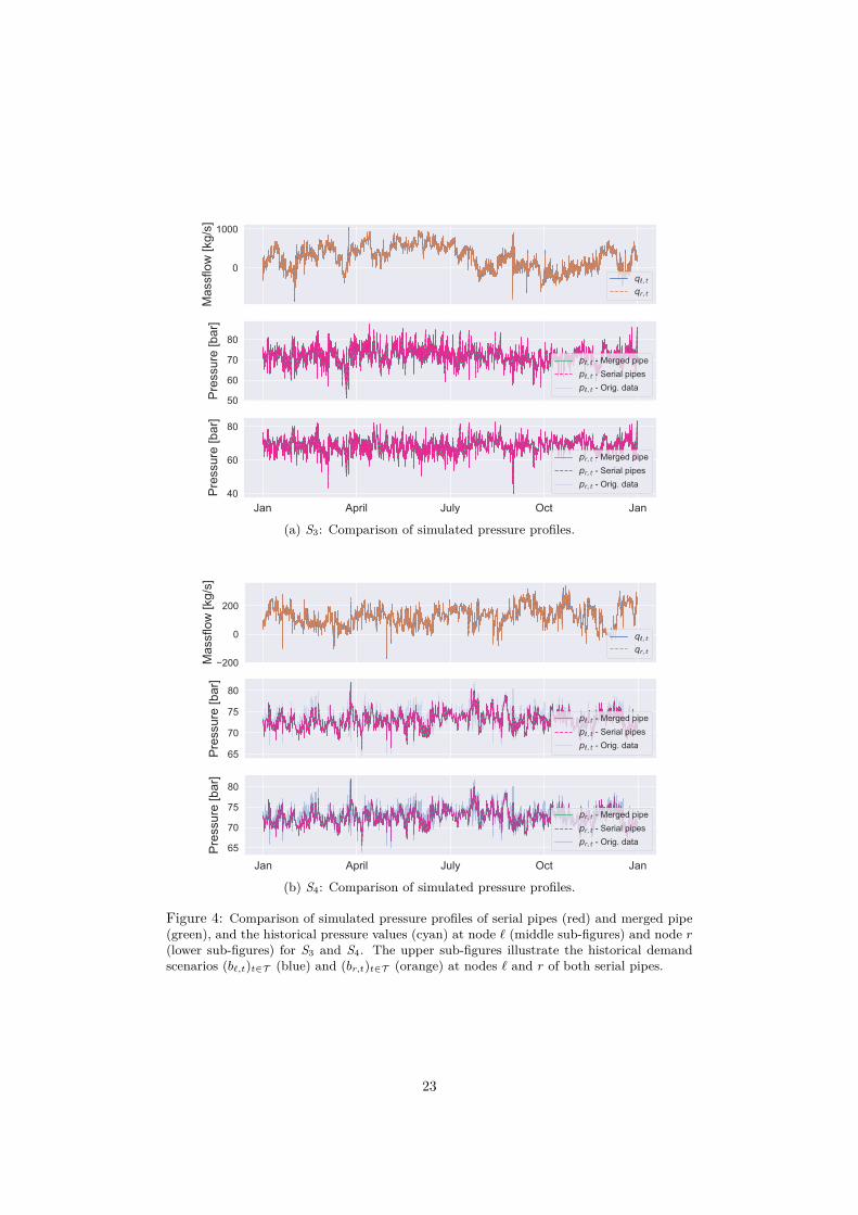
Finally, the middle and lower Sub-figures 3- 5 visualize the simulated pressureprofiles of the serial pipes (red) and the merged pipe (green) at node ` (middlesub-figures) and node r (lower sub-figures). These figures additionally depict thehistorical pressure profiles at both nodes in cyan.

6.4 Relation of transient and stationary serial pipe mergingWe know from Section 5 that the parallel merge allows us to determine pipe param-eters for the merged pipe that preserve the flow and pressure profiles of the parallel

21

0

100

200

Mas

sflo

w [k

g/s]

q , t

qr, t

60

70

80

Pres

sure

[bar

]

p , t - Merged pipep , t - Serial pipesp , t - Orig. data

Jan April July Oct Jan

60

70

80

Pres

sure

[bar

]

pr, t - Merged pipepr, t - Serial pipespr, t - Orig. data

(a) S1: Comparison of simulated pressure profiles.

0

100

Mas

sflo

w [k

g/s]

q , t

qr, t

50

60

70

Pres

sure

[bar

]

p , t - Merged pipep , t - Serial pipesp , t - Orig. data

Jan April July Oct Jan

50

60

70

Pres

sure

[bar

]

pr, t - Merged pipepr, t - Serial pipespr, t - Orig. data

(b) S2: Comparison of simulated pressure profiles.

Figure 3: Comparison of simulated pressure profiles of serial pipes (red) and merged pipe(green), and the historical pressure values (cyan) at node ` (middle sub-figures) and node r(lower sub-figures) for S1 and S2. The upper sub-figures illustrate the historical demandscenarios (b`,t)t∈T (blue) and (br,t)t∈T (orange) at nodes ` and r of both serial pipes.

22

0

1000

Mas

sflo

w [k

g/s]

q , t

qr, t

50

60

70

80

Pres

sure

[bar

]

p , t - Merged pipep , t - Serial pipesp , t - Orig. data

Jan April July Oct Jan40

60

80

Pres

sure

[bar

]

pr, t - Merged pipepr, t - Serial pipespr, t - Orig. data

(a) S3: Comparison of simulated pressure profiles.

200

0

200

Mas

sflo

w [k

g/s]

q , t

qr, t

65

70

75

80

Pres

sure

[bar

]

p , t - Merged pipep , t - Serial pipesp , t - Orig. data

Jan April July Oct Jan65

70

75

80

Pres

sure

[bar

]

pr, t - Merged pipepr, t - Serial pipespr, t - Orig. data

(b) S4: Comparison of simulated pressure profiles.

Figure 4: Comparison of simulated pressure profiles of serial pipes (red) and merged pipe(green), and the historical pressure values (cyan) at node ` (middle sub-figures) and node r(lower sub-figures) for S3 and S4. The upper sub-figures illustrate the historical demandscenarios (b`,t)t∈T (blue) and (br,t)t∈T (orange) at nodes ` and r of both serial pipes.

23

0

100

200

Mas

sflo

w [k

g/s]

q , t

qr, t

60

65

70

Pres

sure

[bar

]

p , t - Merged pipep , t - Serial pipespl, t - Orig. data

Jan April July Oct Jan

60

65

70

Pres

sure

[bar

]

pr, t - Merged pipepr, t - Serial pipespr, t - Orig. data

(a) S5: Comparison of simulated pressure profiles.

0

100

200

300

Mas

sflo

w [k

g/s]

q , t

qr, t

60

70

Pres

sure

[bar

]

p , t - Merged pipep , t - Serial pipesp , t - Orig. data

Jan April July Oct Jan

60

70

Pres

sure

[bar

]

pr, t - Merged pipepr, t - Serial pipespr, t - Orig. data

(b) S6: Comparison of simulated pressure profiles.

Figure 5: Comparison of simulated pressure profiles of serial pipes (red) and merged pipe(green), and the historical pressure values (cyan) at node ` (middle sub-figures) and node r(lower sub-figures) for S5 and S6. The upper sub-figures illustrate the historical demandscenarios (b`,t)t∈T (blue) and (br,t)t∈T (orange) at nodes ` and r of both serial pipes.

24

S1 S2 S3 S4 S5 S6no

de` AD 4.07e−02 2.75e−03 5.02e−01 3.73e−02 4.20e−02 6.22e−04

mean AD 8.10e−03 7.53e−04 5.10e−02 2.34e−02 6.03e−03 2.60e−04mean MAD 6.01e−03 5.92e−04 2.00e−02 2.16e−02 3.73e−03 2.23e−04

node

r AD 4.88e−02 2.72e−03 5.13e−01 3.73e−02 3.78e−02 8.36e−04mean AD 8.30e−03 7.44e−04 4.04e−02 2.29e−02 6.12e−03 3.53e−04mean MAD 6.16e−03 5.83e−04 2.10e−02 2.06e−02 3.81e−03 3.00e−04

Table 2: Difference of simulated pressure values between the serial pipes and the mergedpipe for all six examples S1,S2,S3,S4,S5,S6 stated at nodes ` and r in [bar].

pipelines in the stationary and transient case. However, when merging serial pipesin the transient case, this property is in general not true, as we have seen in Ex-ample 6.6. Nevertheless Corollary 6.5 reveals that “stationary” assumptions enableus to determine such a pipe parameter. While this corollary restricts to horizontalpipes, we show in the remainder of this section that this property also holds fornon-horizontal pipelines in the stationary case.

Again, we distinguish between stationary parameters γst, βst and transient pa-rameters γtr, βtr, as done for parallel pipe merging in Section 5. The followingproposition formalizes the concept of serial merging in the stationary setting. Previ-ous versions for serial merging of horizontal pipes can be found in Lenz and Schwarz(2016) and Groß et al. (2019). Here, we generalize these results by additionallyaccounting for the difference in height along the pipes.

Proposition 6.7. Given two serial pipes a = (`, r), b = (`, r) with pipe characteris-tics γsta , γstb > 0 and βsta , β

stb ≥ 0 respectively and bm = 0, deg (m) = 2. Then, both

pipes can equivalently be replaced by an artificial pipe c = (`, r) with

βstc = βsta βstb and γstc = γsta + βsta γstb .

Proof. From bm = 0 and deg(m) = 2 follows qc := qa = qb. For two pipes in serial,each one is represented by a single Equation (30):

p2` − βsta p2

m + γsta qc|qc| = 0 (56)p2m − βstb p2

r + γstb qc|qc| = 0. (57)

Then, it follows(57)⇒ βsta p2

m − βsta βstb p2r + βsta γbqc|qc| = 0 (58)

(56),(58)⇒ p2` − βsta p2

m + βsta p2m − βsta βstb p2

r + (γsta + βsta γstb ) qc|qc| = 0⇒ p2

` − βsta βstb p2r + (γsta + βsta γstb ) qc|qc| = 0

⇒ βstc = βsta βstb and γstc = γsta + βsta γstb . (59)

In the stationary case, horizontal serial pipes hold βsta = βstb = 1, see Fugenschuhet al. (2015), then from (59) directly follows

βstc = 1 and γstc = γsta + γstb , (60)

which coincides with the formula provided in Corollary 6.5 for transient serial mergesunder “stationary” conditions.

25

7 ConclusionIn this paper, we studied the merge of parallel and serial pipelines in transient gasnetworks. First, we introduced the concept of equivalent and heuristic subnetworkreplacements. Equivalent replacements allow to recover a solution for the originalsubnetwork from the solution of the aggregated (merged) subnetwork. This is ageneric concept and can thus be applied to other aggregation methods than pipemerging.

It turned out that the parallel merge is an equivalent replacement, whereas theserial merge is a heuristic method. Therefore, we evaluated the serial pipe merge ina huge empirical study based on real-world fine-grained state data covering an entireyear taken from the German gas network. Besides the equivalent parallel merge,we found that the serial merge only leads to small errors. We thus conclude thatthe presented serial merge can be considered as appropriate aggregation methods forreal-world transient gas flow problems.

Finally, we remark that the used pipe modeling from Section 2 forms the basisof the presented merging methods. Hence, an interesting avenue for future researchwould be to investigate whether it is possible to derive an appropriate discretization ofthe Euler system (1) that leads to equivalent replacements for both merging methodssimultaneously.

8 AcknowledgementsThis work was supported by the Research Campus MODAL (Mathematical Opti-mization and Data Analysis Laboratories) funded by the German Federal Ministryof Education and Research (fund number 05M14ZAM).

ReferencesAalto H (2015) Model predictive control of natural gas pipeline systems - a case for

constrained system identification. IFAC-PapersOnLine 48(30):197–202

Bales P, Kolb O, Lang J (2009) Hierarchical modelling and model adaptivity for gasflow on networks. In: Allen G, Nabrzyski J, Seidel E, van Albada G, Dongarra J,Sloot P (eds) International Conference on Computational Science, Springer, vol5544, pp 337–346, doi:10.1007/978-3-642-01970-8 33

Brouwer J, Gasser I, Herty M (2011) Gas pipeline models revisited: model hierar-chies, nonisothermal models, and simulations of networks. Multiscale Modeling &Simulation 9(2):601–623

Burlacu R, Egger H, Groß M, Martin A, Pfetsch ME, Schewe L, Sirvent M, SkutellaM (2019) Maximizing the storage capacity of gas networks: a global MINLPapproach. Optimization and Engineering 20(2):543–573, doi:10.1007/s11081-018-9414-5

Carvalho R, Buzna L, Bono F, Gutierrez E, Just W, Arrowsmith D (2009)Robustness of trans-european gas networks. Physical Review E 80(1):016106,doi:10.1103/PhysRevE.80.016106

26

Clees T, Nikitin I, Nikitina L, Segiet L (2018) Modeling of gas compressors and hier-archical reduction for globally convergent stationary network solvers. InternationalJournal On Advances in Systems and Measurements 11(2):61–71

Domschke P, Kolb O, Lang J (2015) Adjoint-based error control for the simulationand optimization of gas and water supply networks. Applied Mathematics andComputation 259:1003–1018

Domschke P, Hiller B, Lang J, Tischendorf C (2017) Modellierung von Gasnetzw-erken: Eine Ubersicht. Tech. rep., Technische Universitat Darmstadt

Ehrhardt K, Steinbach MC (2005) Nonlinear optimization in gas networks. In: Mod-eling, simulation and optimization of complex processes, Springer, pp 139–148,doi:10.1007/3-540-27170-8 11

Fugenschuh A, Geißler B, Gollmer R, Morsi A, Pfetsch ME, Rovekamp J, SchmidtM, Spreckelsen K, Steinbach MC (2015) Physical and technical fundamentalsof gas networks. In: Koch T, Hiller B, Pfetsch ME, Schewe L (eds) Evalu-ating Gas Network Capacities, SIAM-MOS Series on Optimization, pp 17–44,doi:10.1137/1.9781611973693.ch2

Gamrath G, Anderson D, Bestuzheva K, Chen WK, Eifler L, Gasse M, GemanderP, Gleixner A, Gottwald L, Halbig K, Hendel G, Hojny C, Koch T, Le Bodic P,Maher SJ, Matter F, Miltenberger M, Muhmer E, Muller B, Pfetsch M, Schlosser F,Serrano F, Shinano Y, Tawfik C, Vigerske S, Wegscheider F, Weninger D, Witzig J(2020) The SCIP Optimization Suite 7.0. ZIB-Report 20-10, Zuse Institute Berlin,URL https://nbn-resolving.de/urn:nbn:de:0297-zib-78023

Geißler B, Morsi A, Schewe L, Schmidt M (2015) Solving power-constrained gas transportation problems using an MIP-based alternat-ing direction method. Computers & Chemical Engineering 82:303–317,doi:10.1016/j.compchemeng.2015.07.005

Groß M, Pfetsch ME, Schewe L, Schmidt M, Skutella M (2019) Algorithmic re-sults for potential-based flows: Easy and hard cases. Networks 73(3):306–324,doi:10.1002/net.21865

Hahn M, Leyffer S, Zavala VM (2017) Mixed-Integer PDE-constrained optimal con-trol of gas networks. Mathematics and Computer Science

Hastie T, Tibshirani R, Friedman J (2009) The Elements of Statistical Learning,2nd edn. Springer Series in Statistics, New York, URL http://web.stanford.edu/˜hastie/ElemStatLearn/

Hennings F, Anderson L, Hoppmann K, Turner M, Koch T (2019) Controllingtransient gas flow in real-world pipeline intersection areas. Tech. Rep. 19-24,ZIB, Takustr. 7, 14195 Berlin, URL https://nbn-resolving.de/urn:nbn:de:0297-zib-73645

Koch T, Hiller B, Pfetsch ME, Schewe L (2015) Evaluating Gas Network Capacities.SIAM-MOS Series on Optimization, doi:10.1137/1.9781611973693

Korneyenko N (1994) Combinatorial algorithms on a class of graphs. Discrete AppliedMathematics 54(2-3):215–217, doi:10.1016/0166-218X(94)90022-1

27

Lenz R (2021) Optimization of stationary expansion planning and transient networkcontrol by mixed-integer nonlinear programming. PhD thesis, Technische Univer-sitat Berlin

Lenz R, Schwarz R (2016) Optimal looping of pipelines in gas networks. Tech. Rep.16-67, ZIB, Takustr. 7, 14195 Berlin, URL https://nbn-resolving.de/urn:nbn:de:0297-zib-61564

LeVeque RJ (2002) Finite volume methods for hyperbolic problems, vol 31. Cam-bridge university press

Leys C, Ley C, Klein O, Bernard P, Licata L (2013) Detecting outliers: Do not usestandard deviation around the mean, use absolute deviation around the median.Journal of Experimental Social Psychology 49(4):764–766

Liu E, Kuang J, Peng S, Liu Y (2019) Transient operation optimization technologyof gas transmission pipeline: A case study of west-east gas transmission pipeline.IEEE Access 7:112131–112141

Moritz S (2007) A mixed integer approach for the transient case of gas networkoptimization. PhD thesis, Technische Universitat Darmstadt

Nikuradse J (1950) Laws of flow in rough pipes, vol 2. National Advisory Committeefor Aeronautics

Pfetsch ME, Fugenschuh A, Geißler B, Geißler N, Gollmer R, Hiller B, HumpolaJ, Koch T, Lehmann T, Martin A, Morsi A, Rovekamp J, Schewe L, SchmidtM, Schultz R, Schwarz R, Schweiger J, Stangl C, Steinbach MC, Vigerske S,Willert BM (2015) Validation of nominations in gas network optimization: mod-els, methods, and solutions. Optimization Methods and Software 30(1):15–53,doi:10.1080/10556788.2014.888426

Rıos-Mercado RZ, Wu S, Scott LR, Boyd EA (2002) A reduction technique for nat-ural gas transmission network optimization problems. Annals of Operations Re-search 117(1-4):217–234, doi:10.1023/A:1021529709006

Saleh J (2002) Fluid flow handbook. McGraw-Hill Professional, New York

Schmidt M, Aßmann D, Burlacu R, Humpola J, Joormann I, Kanelakis N, KochT, Oucherif D, Pfetsch ME, Schewe L, Schwarz R, Sirvent M (2017) GasLib – ALibrary of Gas Network Instances. Data 2(4):article 40, doi:10.3390/data2040040

Steinbach MC (2007) On PDE solution in transient optimization of gas net-works. Journal of computational and applied mathematics 203(2):345–361,doi:10.1016/j.cam.2006.04.018

Takamizawa K, Nishizeki T, Saito N (1982) Linear-time computability ofcombinatorial problems on series-parallel graphs. J ACM 29(3):623–641,doi:10.1145/322326.322328

Weltsch A (2018) Fast approximation of equations of transient gasflow. Master thesis,Technische Universitat Berlin, Germany

Wilkinson J, Holliday D, Batey E, Hannah K (1964) Transient flow in natural gastransmission systems. American Gas Association, New York p 115

28

Zlotnik A, Dyachenko S, Backhaus S, Chertkov M (2015) Model reduction and op-timization of natural gas pipeline dynamics. In: Dynamic Systems and ControlConference, American Society of Mechanical Engineers, doi:10.1115/DSCC2015-9683

29