
Piezoelectric Floating Element Shear Stress
Sensor for the Wind Tunnel Flow Measurement
Taeyang Kim1, Aditya Saini1, Jinwook Kim1, Ashok Gopalarathnam1, Yong Zhu1,
Frank L. Palmieri2, Christopher J. Wohl2, and Xiaoning Jiang1
1 Department of Mechanical and Aerospace Engineering, North Carolina State University, Raleigh, NC 27695, USA 2 NASA Langley Research Center, Hampton, VA 23681, USA
E-mail: [email protected]
Abstract
A piezoelectric sensor with a floating element was developed for direct measurement of flow
induced shear stress. The piezoelectric sensor was designed to detect the pure shear stress while
suppressing the effect of normal stress generated from the vortex lift-up by applying opposite
poling vectors to the piezoelectric elements. During the calibration stage, the prototyped sensor
showed a high sensitivity to shear stress (91.3 ± 2.1 pC/Pa) due to the high piezoelectric
coefficients (d31=–1330 pC/N) of the constituent 0.67Pb(Mg1∕3Nb2∕3)O3-0.33PbTiO3 (PMN-
33%PT) single crystal. By contrast, the sensor showed almost no sensitivity to normal stress (less
than 1.2 pC/Pa) because of the electromechanical symmetry of the sensing structure. The usable
frequency range of the sensor is up to 800 Hz. In subsonic wind tunnel tests, an analytical model
was proposed based on cantilever beam theory with an end-tip-mass for verifying the resonance
frequency shift in static stress measurements. For dynamic stress measurements, the signal-to-
noise ratio (SNR) and ambient vibration-filtered pure shear stress sensitivity were obtained
through signal processing. The developed piezoelectric shear stress sensor was found to have an
SNR of 15.8 ± 2.2 dB and a sensitivity of 56.5 ± 4.6 pC/Pa in the turbulent flow.
1. Introduction
The measurement of wall shear stress due to flow past solid surfaces provides important
information about flow phenomena, including viscous drag, the transition to turbulence, and flow
separation [1]. Therefore, the capability to measure both temporally and spatially resolved wall

shear stress is important not only from the standpoint of research on basic fluid mechanics, but
also from the perspective of flow control.
Techniques for measuring the shear stress can be categorized into indirect and direct methods
[2]. In indirect methods, the shear stress is extracted from the measurement of other flow properties
(e.g., pressure and wall temperature) that are related to the shear stress. For example, Pitot tubes
such as the Preston tube or Stanton tube use a stream-based distribution of pressure along a flow
channel to derive the shear stress [3]–[5]. The major disadvantage of the Pitot tube method is that
using the ports for pressure measurements requires modification to the wall, presenting a potential
disturbance to the flow. Another common indirect method is the ‘hot film technique’ which is
based on the thermal transfer principle [6]–[9]. Compared with Pitot tube measurement techniques,
thermal sensors cause less disturbance to the flow because the sensor is mounted flush with the
surface. However, they suffer from severe sources of error due to interference arising from
surrounding humidity and temperature.
Considering the limitations of indirect methods, which strongly depend on empirical laws
[2], direct methods are more accurate for measuring shear stress in complex, difficult-to-model
flows [10]. Direct measurement relies on detecting the total amount of viscous drag that a surface-
mounted force sensor experiences. An example of the direct measurement method is the floating
element (FE) sensor, which is based on measuring the displacement of a FE that is flush with the
flow. Capacitive [11]–[14] and piezoresistive [15], [16] techniques as well as surface acoustic
wave (SAW) devices [17], [18] have been developed and used to measure the displacement of a
FE. However, shear stress sensors fabricated by micro-machining have not yet received sufficient
validation in a turbulent flow environment, so further advancement is needed to obtain reliable,
high resolution shear stress measurements that are applicable to a wide range of flows.
This paper details a low cost small piezoelectric (PE) floating-element-type sensor
(10×10×20 mm3) that was developed using relatively facile techniques. A PMN-33%PT crystal
was used in the sensor for its high PE coefficient (d31=–1330 pC/N) [20], [21]. The proposed sensor
was specifically designed to be both resilient against normal stresses that are generated from the
vortex lift-up in the wind tunnel, and to prevent potential errors due to misalignments between the
FE and the test plate. Finally, deflection of the PE sensing element was observed in wind tunnel
testing. The static shear stress amplitude, that is the low frequency component of the shear stress,
was determined through analytical modeling (cantilever beam theory) of the change in resonance
frequency of the PE sensing element that would arise from deflection. The variation in charge
output from the PE sensor was utilized to determine the dynamic shear stress in the turbulent flow
condition.
In this paper, the sensor design and fabrication are described (Section 2). Experimental
methods are presented and a dynamic calibration setup for the sensor and the wind tunnel model
is illustrated in Section 3. Based on this experimental configuration, an analytical model for static
stress is proposed and additional devices such as trip-strips and Pitot tubes are introduced for
dynamic stress measurement. In section 4, results are presented, which include the characterization
of the fabricated sensor and discussion of static and dynamic stress measurements. Finally, we
conclude this paper with a brief summary in Section 5.
2. Sensor design and fabrication
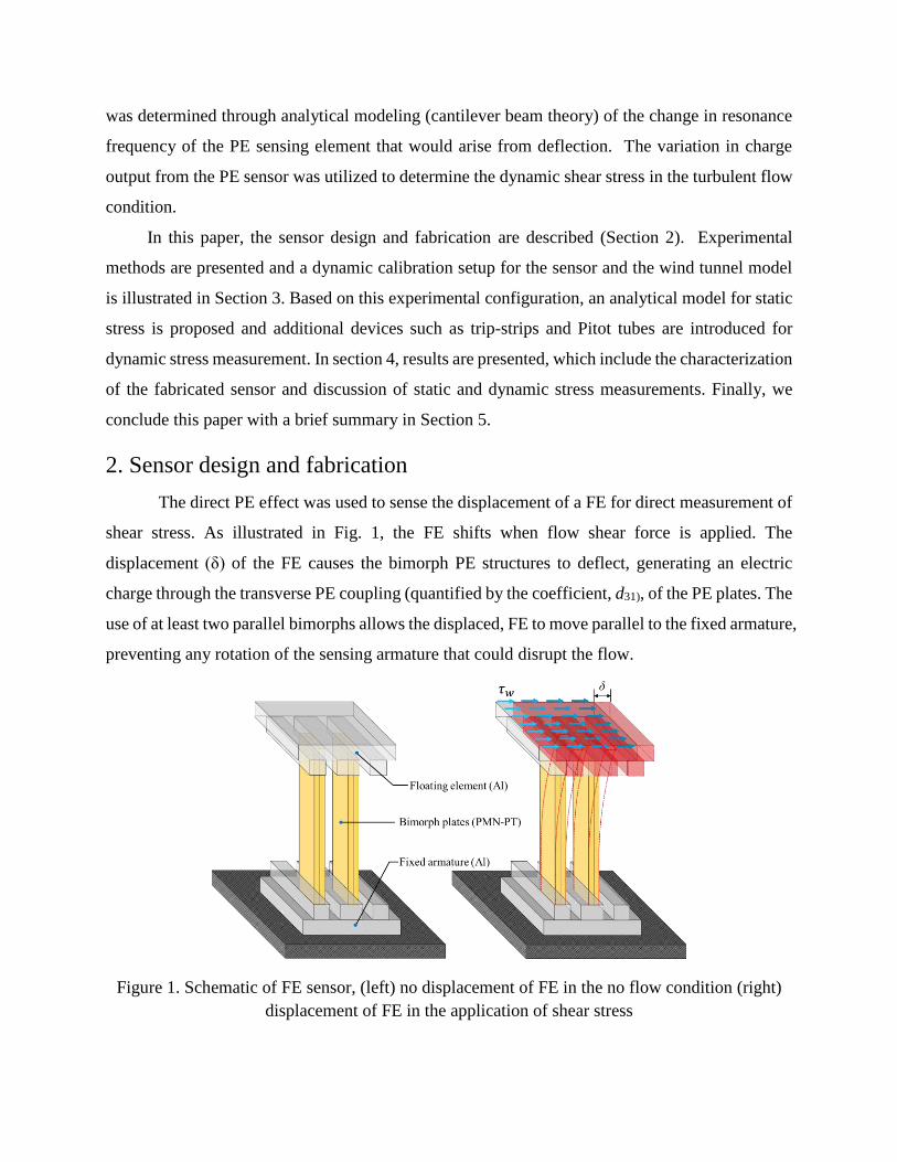
The direct PE effect was used to sense the displacement of a FE for direct measurement of
shear stress. As illustrated in Fig. 1, the FE shifts when flow shear force is applied. The
displacement (δ) of the FE causes the bimorph PE structures to deflect, generating an electric
charge through the transverse PE coupling (quantified by the coefficient, d31), of the PE plates. The
use of at least two parallel bimorphs allows the displaced, FE to move parallel to the fixed armature,
preventing any rotation of the sensing armature that could disrupt the flow.
Figure 1. Schematic of FE sensor, (left) no displacement of FE in the no flow condition (right)
displacement of FE in the application of shear stress
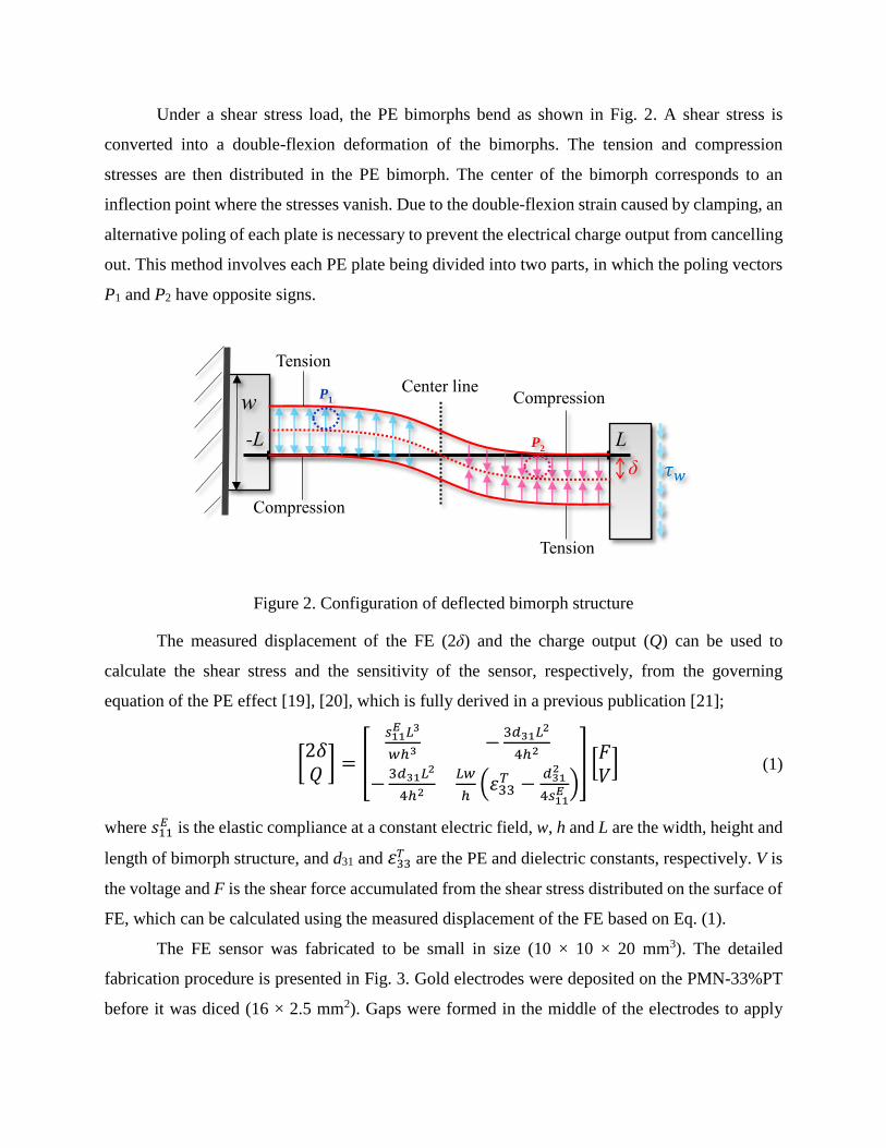
Under a shear stress load, the PE bimorphs bend as shown in Fig. 2. A shear stress is
converted into a double-flexion deformation of the bimorphs. The tension and compression
stresses are then distributed in the PE bimorph. The center of the bimorph corresponds to an
inflection point where the stresses vanish. Due to the double-flexion strain caused by clamping, an
alternative poling of each plate is necessary to prevent the electrical charge output from cancelling
out. This method involves each PE plate being divided into two parts, in which the poling vectors
P1 and P2 have opposite signs.
Figure 2. Configuration of deflected bimorph structure
The measured displacement of the FE (2δ) and the charge output (Q) can be used to
calculate the shear stress and the sensitivity of the sensor, respectively, from the governing
equation of the PE effect [19], [20], which is fully derived in a previous publication [21];
[2𝛿𝑄
] = [
𝑠11𝐸 𝐿3
𝑤ℎ3−
3𝑑31𝐿2
4ℎ2
−3𝑑31𝐿2
4ℎ2
𝐿𝑤
ℎ(휀33
𝑇 −𝑑31
2
4𝑠11𝐸 )
] [𝐹𝑉
] (1)
where 𝑠11𝐸 is the elastic compliance at a constant electric field, w, h and L are the width, height and
length of bimorph structure, and d31 and 휀33𝑇 are the PE and dielectric constants, respectively. V is
the voltage and F is the shear force accumulated from the shear stress distributed on the surface of
FE, which can be calculated using the measured displacement of the FE based on Eq. (1).
The FE sensor was fabricated to be small in size (10 × 10 × 20 mm3). The detailed
fabrication procedure is presented in Fig. 3. Gold electrodes were deposited on the PMN-33%PT
before it was diced (16 × 2.5 mm2). Gaps were formed in the middle of the electrodes to apply
L -L
δ
Center line
𝜏𝑤
Tension
Compression
w
Tension
Compression
P2
P1

opposite poling vectors to the underlying plates. The poled plates were bonded as series mode
bimorphs using an epoxy resin (Epotek 301), which ensured the higher sensitivity of the sensors
in comparison with the parallel mode connection [19].
Figure 3. Sensor fabrication procedure
The final prototype of the sensor consists of the floating element (top), the clamped element
(bottom) with an aluminum plate, two bimorph plates of PMN-33%PT crystals in a series
combination, and a protective housing (Fig. 4).
Figure 4. Configuration of PE sensor (a) isometric (b) front view (c) with housing. Demarcation
on the ruler included in images (a) and (b) are mm.

Another important consideration taken into account during the design of the FE type
sensors was the presence of errors caused by sensor misalignments. Misalignment errors originate
from the geometry of the FE and the gap surrounding it. When the element is misaligned, pressures
acting on the lip and surface of the element create moments which erroneously become part of the
wall shear measurement [22]. Some comprehensive studies on misalignment error have been
conducted by Allen et al. [23], [24] in which they state that while a perfectly aligned FE would
have minimal error, optimizing different geometric parameters could effectively reduce the errors
caused by misalignment. They identified three key geometric parameters: misalignment (Z), gap
size (G), and lip size (L). These parameters are illustrated in Fig. 5. To prevent or/and minimize
likely errors from the misalignment between the FE and the test plate, several design
considerations were taken into account for the sensors generated in this work. [22]–[25].
The protective housing: A protective collar component surrounding the FE, if carefully
aligned with the FE, can significantly mitigate the effects associated with the sensor
misalignment (Z) during a facility installation.
Gap size (G) between the FE and housing (200 μm): A sensor with a small gap size is
much more prone to misalignment error. The optimum ratio of gap (G) to length of FE
was found to be 0.02 through the experimental validation.
Lip size (L) of the FE: This was intentionally minimized (1 mm) based on the total height
of the FE (3 mm) to reduce the area on which the pressures had to act in the case of
misalignment.
Figure 5. Key parameters of the FE to minimize the potential errors

3. Experimental methods
3.1. Dynamic calibration
A calibration setup was assembled to characterize the fabricated sensor. Fig. 6(a) represents
the experimental setup for the dynamic calibration of the sensor. The actuator, excited by a
function generator (Tektronix, Cary, NC) and power amplifier (ValueTronics, Elgin, IL), applied
a low frequency (1 Hz) vibrational displacement to the sensor. A laser vibrometer (Polytec,
Mooresville, NC) was used to measure the displacement of the FE, while an oscilloscope (Agilent
Technologies, Santa Clara, CA) provided a visual display of the displacement profile. The charge
output generated from the bimorph PE plate was measured by the lock-in amplifier (Stanford
Research Systems, Sunnyvale, CA). In this test, the reference frequency (1 Hz) of the lock-in
amplifier was synchronized with the function generator and the excitation force, i.e., displacement
magnitude, was controlled by increasing the voltage amplitude from the function generator in the
range of 0.1 V to 1.0 V with a 0.1 V sub-step.
The dynamic calibrations of the shear stress and normal stress were conducted by positioning the
contact probe of the actuator on the side and top of the FE, respectively. (Fig. 6(b), (c)).
Usable frequency range of the sensor was measured by increasing the reference frequency of the
function generator by 1 Hz up to the phase shift of the sensor.
Figure 6. Experimental setup for the calibration of a sensor in (a) overall view, (b) shear stress,
(c) normal stress

3.2. Wind tunnel model
The characterization of the PE sensors under actual wind-flow conditions was carried out
in a subsonic wind tunnel facility at North Carolina State University (NCSU). The facility enabled
an evaluation of the response from PE sensors by comparing the output signals with aerodynamic
measurements from several traditional approaches.
The test apparatus was a flat plate fabricated from medium density fiberboard (MDF). The
flat plate was 406 mm (16”) in chord, 813 mm (32”) in span and 19.5 mm (¾”) thick. A semi-
circular leading edge was attached to the front edge of the flat plate, and the PE sensor housing
was positioned 229 mm (9”, 0.56 chord) from the leading-edge of the flat plate. Additionally, the
flat-plate model had an extended trailing flap attachment. This movable flap enabled adjustments
in overall pressure distribution over the flat plate, ensuring that the stagnation point was positioned
on the upper surface of the flat plate. Fig. 7 represents the wind tunnel experimental setup for
sensors, in which the PE sensor was flush-mounted on the flat plate and carefully aligned by
adjustable joint bolts. Fig. 8 shows the schematic of the setup for the PE sensor that was mounted
on the test apparatus. Qualitative estimates of the skin friction coefficient and the expected shear
stress on the flat plate were conducted using theoretical and experimental boundary layer analysis
with the Pitot tube apparatus, which will be introduced in Section 3.4 in detail.
Figure 7. Wind tunnel experimental setup (a) side, (b) top and close view
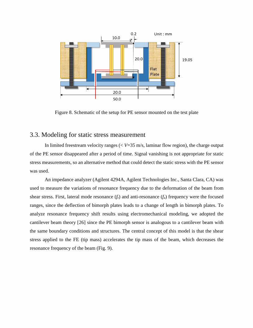
Figure 8. Schematic of the setup for PE sensor mounted on the test plate
3.3. Modeling for static stress measurement
In limited freestream velocity ranges (< V=35 m/s, laminar flow region), the charge output
of the PE sensor disappeared after a period of time. Signal vanishing is not appropriate for static
stress measurements, so an alternative method that could detect the static stress with the PE sensor
was used.
An impedance analyzer (Agilent 4294A, Agilent Technologies Inc., Santa Clara, CA) was
used to measure the variations of resonance frequency due to the deformation of the beam from
shear stress. First, lateral mode resonance (fr) and anti-resonance (fa) frequency were the focused
ranges, since the deflection of bimorph plates leads to a change of length in bimorph plates. To
analyze resonance frequency shift results using electromechanical modeling, we adopted the
cantilever beam theory [26] since the PE bimorph sensor is analogous to a cantilever beam with
the same boundary conditions and structures. The central concept of this model is that the shear
stress applied to the FE (tip mass) accelerates the tip mass of the beam, which decreases the
resonance frequency of the beam (Fig. 9).

Figure 9. Cantilever beam with accelerated tip mass
For a cantilever beam subjected to free vibration, the system is considered to be continuous
with the beam mass distributed along the shaft. The equation of motion for this can be written as
[26]:
(2)
where E is the Young’s modulus of the beam material, I is the moment of inertia in the beam cross-
section, m is the mass per unit length, m = ρA, ρ is the material density, A is the cross-sectional
area, x is the distance measured from the fixed end, y(x) is displacement in y direction at distance
x from fixed end, and ω is the angular natural frequency. Boundary conditions of the cantilever
beam are:
(3)
For a uniform beam under free vibration from Eq. (4), we get:
(4)
The mode shapes for a continuous cantilever beam are given as:
𝑦𝑛(𝑥) = 𝐴𝑛{(𝑠𝑖𝑛𝛽𝑛𝐿 − 𝑠𝑖𝑛ℎ𝛽𝑛𝐿)(𝑠𝑖𝑛𝛽𝑛𝑥 − 𝑠𝑖𝑛ℎ𝛽𝑛𝑥) + (𝑐𝑜𝑠𝛽𝑛𝐿 − 𝑐𝑜𝑠ℎ𝛽𝑛𝐿)(𝑐𝑜𝑠𝛽𝑛𝑥 − 𝑐𝑜𝑠ℎ𝛽𝑛𝑥)},
𝑛 = 1, 2, 3 ⋯ ∞ (5)
From Eq. (5), a closed form of the resonance frequency fn, and the effective mass of beam meff,
without any tip mass can be written as:
𝑑2
𝑑𝑥2{𝐸𝐼(𝑥)
𝑑2𝑦(𝑥)
𝑑𝑥2} = 𝜔2𝑚(𝑥)𝑦(𝑥)
𝑦(0) = 0, 𝑦′(0) = 0, 𝑦′′(𝐿) = 0, 𝑦′′′(𝐿) = 0
𝑑4𝑦(𝑥)
𝑑𝑥4− 𝛽4𝑦(𝑥) = 0, 𝛽4 =
𝜔2𝑚
𝐸𝐼
(6)
(7)
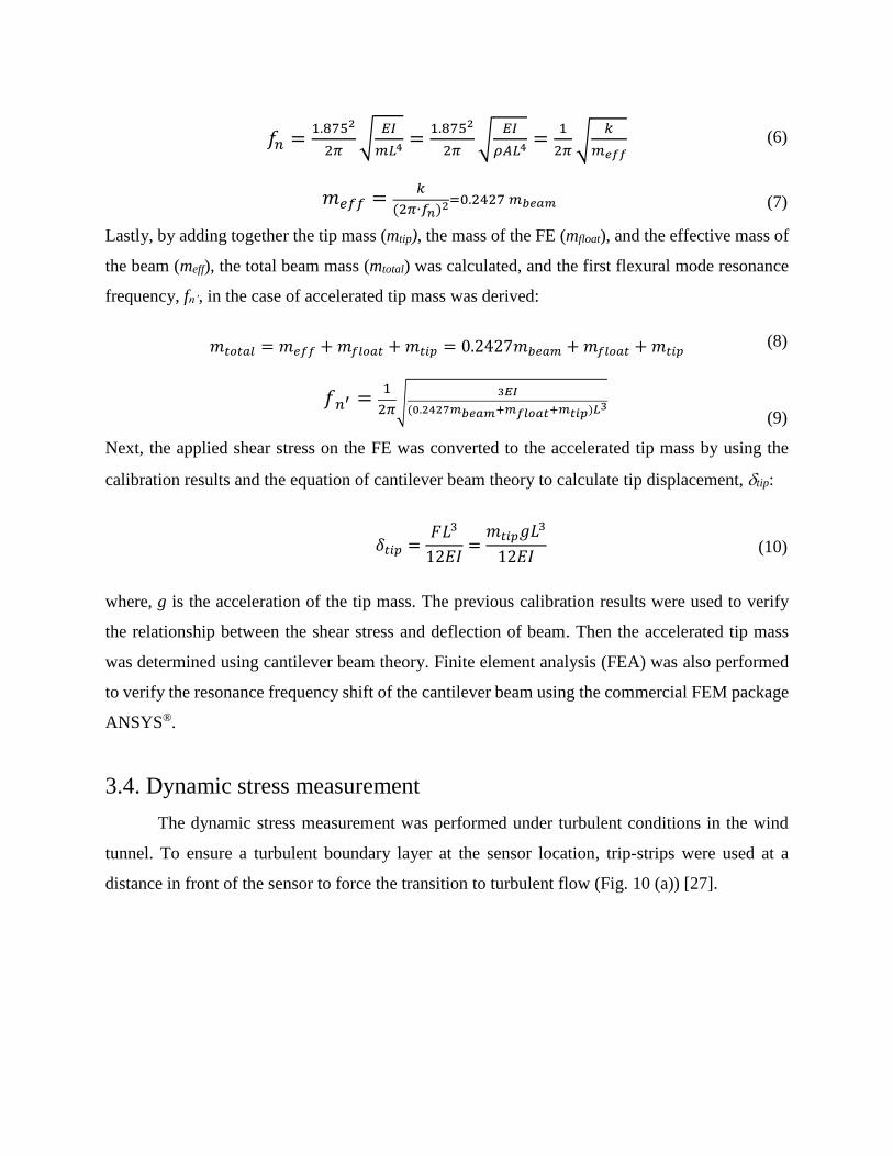
Lastly, by adding together the tip mass (mtip), the mass of the FE (mfloat), and the effective mass of
the beam (meff), the total beam mass (mtotal) was calculated, and the first flexural mode resonance
frequency, fn’, in the case of accelerated tip mass was derived:
(8)
(9)
Next, the applied shear stress on the FE was converted to the accelerated tip mass by using the
calibration results and the equation of cantilever beam theory to calculate tip displacement, tip:
(10)
where, g is the acceleration of the tip mass. The previous calibration results were used to verify
the relationship between the shear stress and deflection of beam. Then the accelerated tip mass
was determined using cantilever beam theory. Finite element analysis (FEA) was also performed
to verify the resonance frequency shift of the cantilever beam using the commercial FEM package
ANSYS®.
3.4. Dynamic stress measurement
The dynamic stress measurement was performed under turbulent conditions in the wind
tunnel. To ensure a turbulent boundary layer at the sensor location, trip-strips were used at a
distance in front of the sensor to force the transition to turbulent flow (Fig. 10 (a)) [27].
𝑓𝑛 =1.8752
2𝜋√
𝐸𝐼
𝑚𝐿4=
1.8752
2𝜋√
𝐸𝐼
𝜌𝐴𝐿4=
1
2𝜋√
𝑘
𝑚𝑒𝑓𝑓
𝑚𝑒𝑓𝑓 =𝑘
(2𝜋∙𝑓𝑛)2=0.2427 𝑚𝑏𝑒𝑎𝑚
𝑚𝑡𝑜𝑡𝑎𝑙 = 𝑚𝑒𝑓𝑓 + 𝑚𝑓𝑙𝑜𝑎𝑡 + 𝑚𝑡𝑖𝑝 = 0.2427𝑚𝑏𝑒𝑎𝑚 + 𝑚𝑓𝑙𝑜𝑎𝑡 + 𝑚𝑡𝑖𝑝
𝑓𝑛′ =1
2𝜋√3𝐸𝐼
(0.2427𝑚𝑏𝑒𝑎𝑚+𝑚𝑓𝑙𝑜𝑎𝑡+𝑚𝑡𝑖𝑝)𝐿3
𝛿𝑡𝑖𝑝 =𝐹𝐿3
12𝐸𝐼=
𝑚𝑡𝑖𝑝𝑔𝐿3
12𝐸𝐼
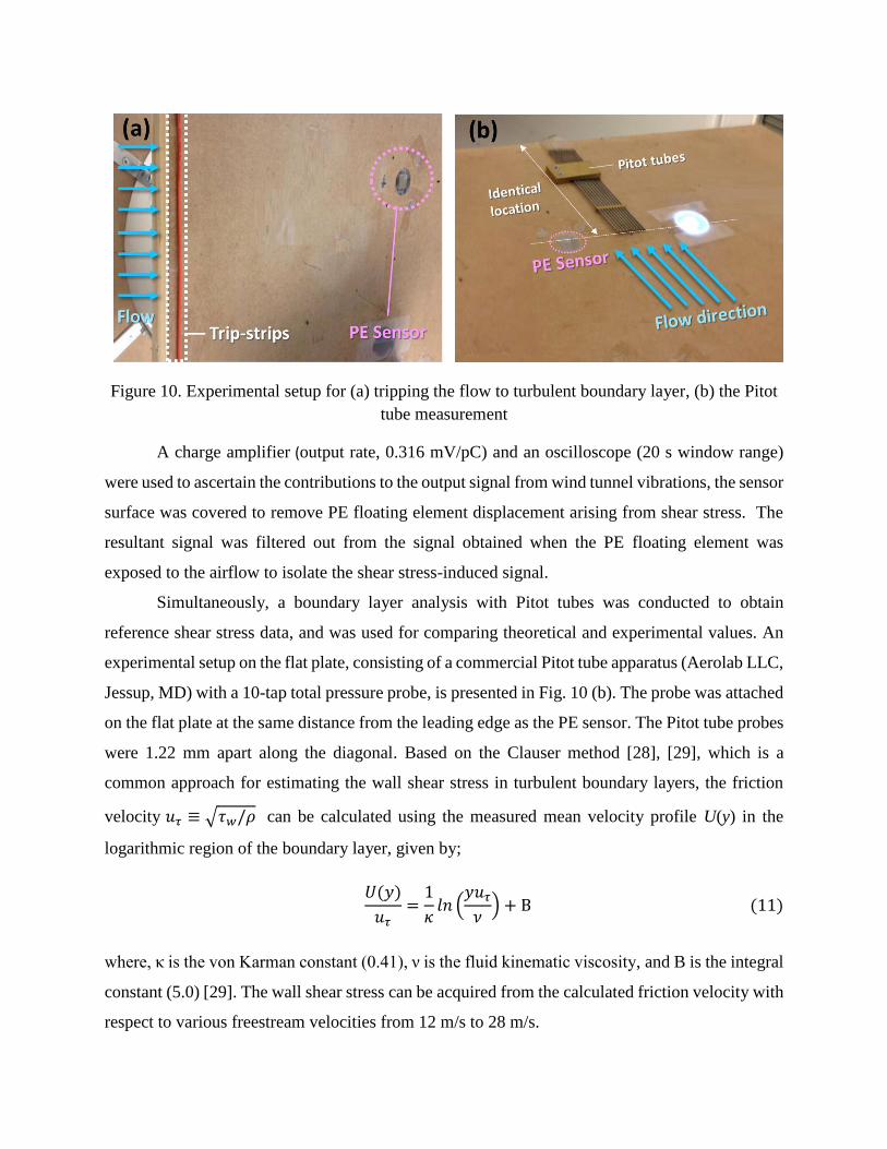
Figure 10. Experimental setup for (a) tripping the flow to turbulent boundary layer, (b) the Pitot
tube measurement
A charge amplifier (output rate, 0.316 mV/pC) and an oscilloscope (20 s window range)
were used to ascertain the contributions to the output signal from wind tunnel vibrations, the sensor
surface was covered to remove PE floating element displacement arising from shear stress. The
resultant signal was filtered out from the signal obtained when the PE floating element was
exposed to the airflow to isolate the shear stress-induced signal.
Simultaneously, a boundary layer analysis with Pitot tubes was conducted to obtain
reference shear stress data, and was used for comparing theoretical and experimental values. An
experimental setup on the flat plate, consisting of a commercial Pitot tube apparatus (Aerolab LLC,
Jessup, MD) with a 10-tap total pressure probe, is presented in Fig. 10 (b). The probe was attached
on the flat plate at the same distance from the leading edge as the PE sensor. The Pitot tube probes
were 1.22 mm apart along the diagonal. Based on the Clauser method [28], [29], which is a
common approach for estimating the wall shear stress in turbulent boundary layers, the friction
velocity 𝑢𝜏 ≡ √𝜏𝑤/𝜌 can be calculated using the measured mean velocity profile U(y) in the
logarithmic region of the boundary layer, given by;
𝑈(𝑦)
𝑢𝜏=
1
𝜅𝑙𝑛 (
𝑦𝑢𝜏
𝜈) + B (11)
where, κ is the von Karman constant (0.41), ν is the fluid kinematic viscosity, and B is the integral
constant (5.0) [29]. The wall shear stress can be acquired from the calculated friction velocity with
respect to various freestream velocities from 12 m/s to 28 m/s.
4. Results and discussions
4.1. Dynamic calibration
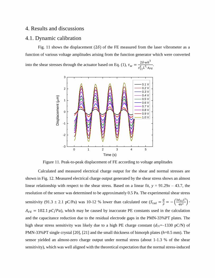
Fig. 11 shows the displacement (2𝛿) of the FE measured from the laser vibrometer as a
function of various voltage amplitudes arising from the function generator which were converted
into the shear stresses through the actuator based on Eq. (1), 𝜏𝑤 =2𝛿∙𝑤ℎ
3
𝑠11𝐸 𝐿3∙𝐴𝐹𝐸
.
Figure 11. Peak-to-peak displacement of FE according to voltage amplitudes
Calculated and measured electrical charge output for the shear and normal stresses are
shown in Fig. 12. Measured electrical charge output generated by the shear stress shows an almost
linear relationship with respect to the shear stress. Based on a linear fit, y = 91.29x – 43.7, the
resolution of the sensor was determined to be approximately 0.5 Pa. The experimental shear stress
sensitivity (91.3 ± 2.1 pC/Pa) was 10-12 % lower than calculated one (𝑆𝑐𝑎𝑙 =𝑄
𝑃= − (
3𝑑31𝐿2
4ℎ2 ) ∙
𝐴𝐹𝐸 = 102.1 𝑝𝐶/𝑃𝑎), which may be caused by inaccurate PE constants used in the calculation
and the capacitance reduction due to the residual electrode gaps in the PMN-33%PT plates. The
high shear stress sensitivity was likely due to a high PE charge constant (d31=–1330 pC/N) of
PMN-33%PT single crystal [20], [21] and the small thickness of bimorph plates (h=0.5 mm). The
sensor yielded an almost-zero charge output under normal stress (about 1-1.3 % of the shear
sensitivity), which was well aligned with the theoretical expectation that the normal stress-induced
0 1 2 3 4 5-3
-2
-1
0
1
2
3
Dis
pla
cem
ent (
m)
Time (s)
0.1 V
0.2 V
0.3 V
0.4 V
0.5 V
0.6 V
0.7 V
0.8 V
0.9 V
1.0 V
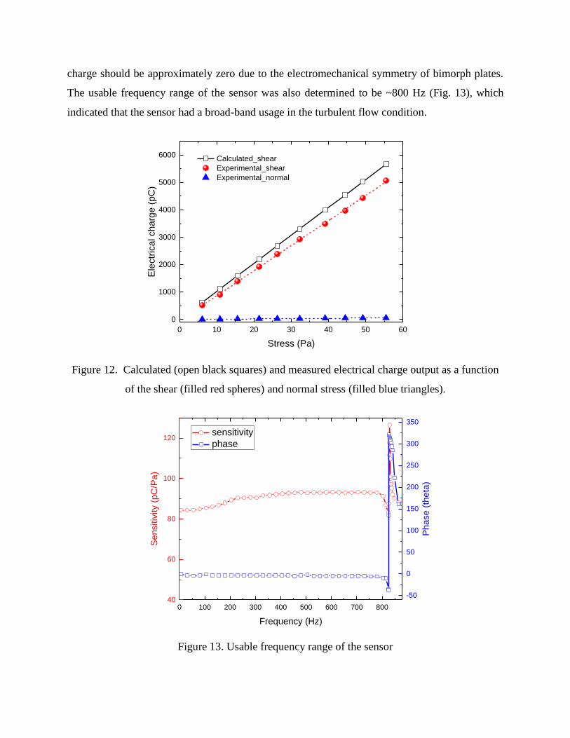
charge should be approximately zero due to the electromechanical symmetry of bimorph plates.
The usable frequency range of the sensor was also determined to be ~800 Hz (Fig. 13), which
indicated that the sensor had a broad-band usage in the turbulent flow condition.
Figure 12. Calculated (open black squares) and measured electrical charge output as a function
of the shear (filled red spheres) and normal stress (filled blue triangles).
Figure 13. Usable frequency range of the sensor
0 100 200 300 400 500 600 700 80040
60
80
100
120 sensitivity
phase
Frequency (Hz)
Sensitiv
ity (
pC
/Pa)
-50
0
50
100
150
200
250
300
350P
hase (
theta
)
0 10 20 30 40 50 60
0
1000
2000
3000
4000
5000
6000E
lectr
ica
l ch
arg
e (
pC
)
Stress (Pa)
Calculated_shear
Experimental_shear
Experimental_normal
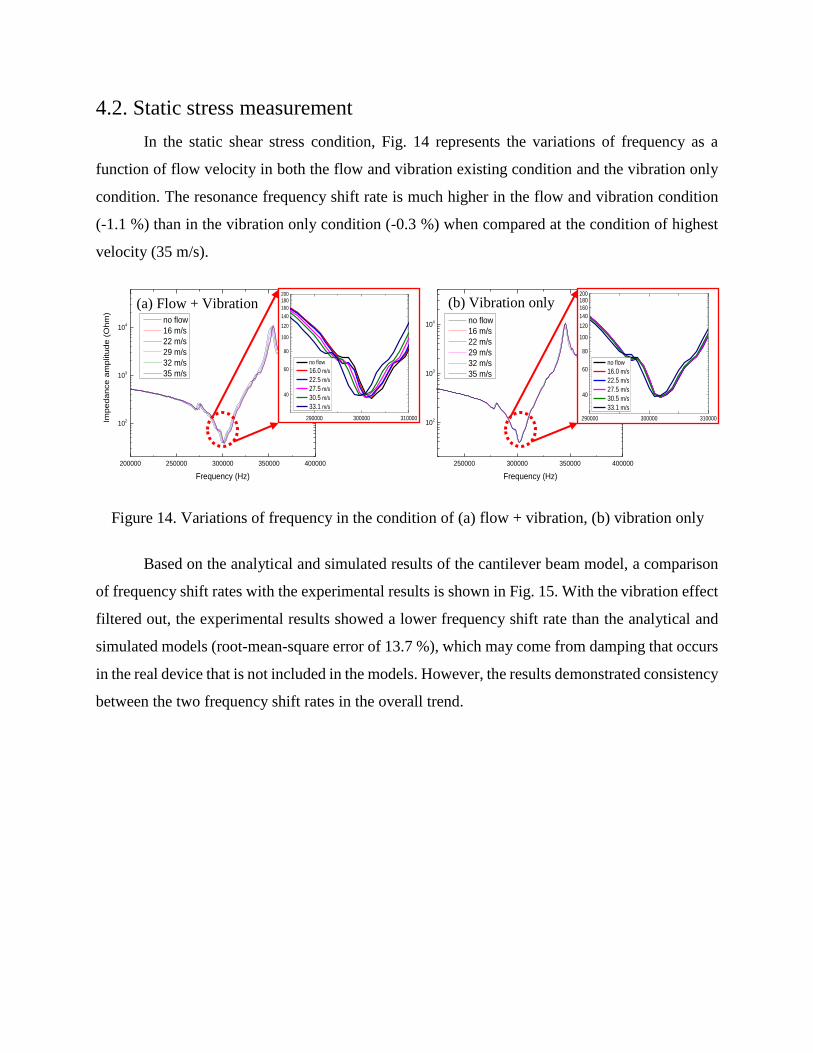
4.2. Static stress measurement
In the static shear stress condition, Fig. 14 represents the variations of frequency as a
function of flow velocity in both the flow and vibration existing condition and the vibration only
condition. The resonance frequency shift rate is much higher in the flow and vibration condition
(-1.1 %) than in the vibration only condition (-0.3 %) when compared at the condition of highest
velocity (35 m/s).
Figure 14. Variations of frequency in the condition of (a) flow + vibration, (b) vibration only
Based on the analytical and simulated results of the cantilever beam model, a comparison
of frequency shift rates with the experimental results is shown in Fig. 15. With the vibration effect
filtered out, the experimental results showed a lower frequency shift rate than the analytical and
simulated models (root-mean-square error of 13.7 %), which may come from damping that occurs
in the real device that is not included in the models. However, the results demonstrated consistency
between the two frequency shift rates in the overall trend.
250000 300000 350000 400000
102
103
104
Impe
da
nce
am
plitu
de (
Oh
m)
Frequency (Hz)
no flow
16 m/s
22 m/s
29 m/s
32 m/s
35 m/s
200000 250000 300000 350000 400000
102
103
104
Impe
da
nce
am
plitu
de (
Oh
m)
Frequency (Hz)
no flow
16 m/s
22 m/s
29 m/s
32 m/s
35 m/s
(a) Flow + Vibration (b) Vibration only
290000 300000 310000
40
60
80
100
120
140
160
180
200
no flow
16.0 m/s
22.5 m/s
27.5 m/s
30.5 m/s
33.1 m/s
290000 300000 310000
40
60
80
100
120
140
160
180200
no flow
16.0 m/s
22.5 m/s
27.5 m/s
30.5 m/s
33.1 m/s
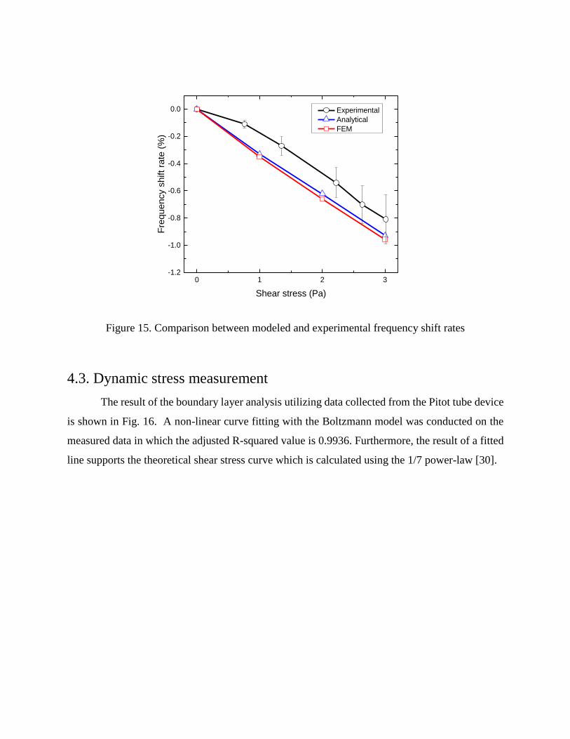
Figure 15. Comparison between modeled and experimental frequency shift rates
4.3. Dynamic stress measurement
The result of the boundary layer analysis utilizing data collected from the Pitot tube device
is shown in Fig. 16. A non-linear curve fitting with the Boltzmann model was conducted on the
measured data in which the adjusted R-squared value is 0.9936. Furthermore, the result of a fitted
line supports the theoretical shear stress curve which is calculated using the 1/7 power-law [30].
0 1 2 3-1.2
-1.0
-0.8
-0.6
-0.4
-0.2
0.0
Fre
quency s
hift ra
te (
%)
Shear stress (Pa)
Experimental
Analytical
FEM

Figure 16. Comparison in the shear stress between the Pitot tubes measurement and the
theoretical analysis
Based on the dynamic stress experimental setup, the shear stress effect on the sensor was
verified under turbulent flow conditions by comparing the peak-to-peak charge outputs of
condition #1 (flow + vibration) and condition #2 (vibration only). As the freestream velocity
increased, peak-to-peak charge outputs at both conditions also increased. However, higher peak-
to-peak charge outputs were observed under condition #1 relative to condition #2, which indicated
that the sensor was able to detect the dynamic shear stress, albeit convolved with signals arising
from wind tunnel vibrations (Fig. 17).
12 14 16 18 20 22 24 26 280.0
0.5
1.0
1.5
2.0
2.5
Shear
str
ess @
x =
0.2
28 m
(P
a)
Freestream velocity (m/s)
Theoretical curve (1/7 power-law)
Pitot tubes data
Non-linear fitting curve (Boltzmann)
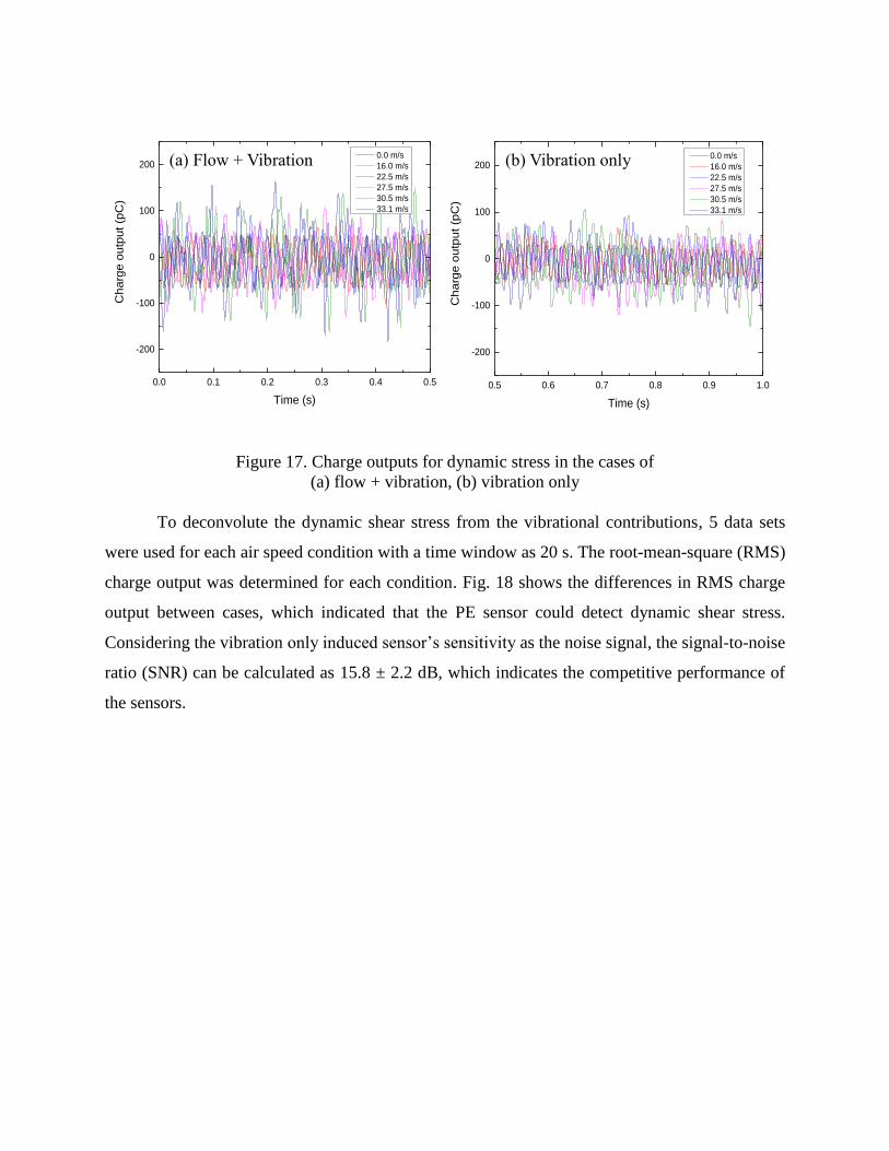
Figure 17. Charge outputs for dynamic stress in the cases of
(a) flow + vibration, (b) vibration only
To deconvolute the dynamic shear stress from the vibrational contributions, 5 data sets
were used for each air speed condition with a time window as 20 s. The root-mean-square (RMS)
charge output was determined for each condition. Fig. 18 shows the differences in RMS charge
output between cases, which indicated that the PE sensor could detect dynamic shear stress.
Considering the vibration only induced sensor’s sensitivity as the noise signal, the signal-to-noise
ratio (SNR) can be calculated as 15.8 ± 2.2 dB, which indicates the competitive performance of
the sensors.
0.0 0.1 0.2 0.3 0.4 0.5
-200
-100
0
100
200
Ch
arg
e o
utp
ut
(pC
)
Time (s)
0.0 m/s
16.0 m/s
22.5 m/s
27.5 m/s
30.5 m/s
33.1 m/s
0.5 0.6 0.7 0.8 0.9 1.0
-200
-100
0
100
200
Charg
e o
utp
ut (p
C)
Time (s)
0.0 m/s
16.0 m/s
22.5 m/s
27.5 m/s
30.5 m/s
33.1 m/s
(a) Flow + Vibration (b) Vibration only

0.5 1.0 1.5 2.0 2.5 3.090
100
110
120
130
140
150
160
170
180
Ch
arg
e o
utp
ut_
RM
S (
pC
)
Shear stress (Pa)
Flow+Vibration
Vibration only
Figure 18. RMS charge outputs between case #1 and #2
To get the pure shear stress data, we filtered out the vibration induced noise by subtracting
the vibration charge outputs, which is shown in Fig. 19.
Figure 19. Comparison in charge outputs between test and calibration data
0.5 1.0 1.5 2.0 2.5 3.00
50
100
150
200
250
Charg
e o
utp
ut (p
C)
Shear stress (Pa)
Wind tunnel test data
Calibration data

Compared with dynamic calibration data, wind tunnel test data exhibited lower charge
outputs, approximately 20 to 27 %, than those obtained in the calibration experiments. This
suggests that the wind tunnel vibrational contribution to the signal may reduce the sensitivity of
the sensor. The frequency spectrum of vibration in the sensor higher than 800 Hz may cause the
sensor performance to degrade. However, sensitivity of the sensor remains high (56.5 ± 4.6 pC/Pa),
and when considering various uncontrollable parameters in the wind tunnel, such as temperature
and vibration, it presented comparable results.
5. Conclusion
In this work, a PE floating element type shear stress sensor was developed, calibrated and
tested in a wind tunnel. The sensor was designed to minimize misalignment error by using a
protective housing, optimizing the gap size, and minimizing the lip size. The sensor was also
designed to be resilient against normal stresses generated from the vortex lift-up so that pure shear
stress could be measured. The calibration results showed that the sensor yielded high shear stress
sensitivity due to the high PE charge constant (d31) of the PMN-33%PT single crystal and small
thickness of the plates, while showing minimal sensitivity to normal stress. In subsonic wind tunnel
tests, electromechanical modeling was performed based on the cantilever beam theory for
verifying the results of the resonance frequency shift in the static stress condition. The sensor was
found to have an SNR of 15.8 ± 2.2 dB and a high sensitivity of 56.5 ± 4.6 pC/Pa in the turbulent
flow.
6. Acknowledgment
This research was supported by the National Aeronautics and Space Administration
(NASA) under contract # NNX14AN42A.

7. References
[1] A. J. Smits and J.-P. Dussauge, Turbulent shear layers in supersonic flow, 2nd ed. New
York: Springer, 2006.
[2] Joseph H. Haritonidis, “The measurement of wall shear stress,” Adv. Fluid Mech. Meas.,
vol. 45, pp. 229–261, 1989.
[3] J. P. Preston, “The Determination of Turbulent Skin Friction by Means of Pitot Tubes,” J.
R. Aeronaut. Soc., vol. 58, pp. 109–121, 1954.
[4] J. N. Hool, “Measurement of Skin Friction Using Surface Tubes,” Aircr. Eng. Aerosp.
Technol., vol. 28, no. 2, pp. 52–54, 1956.
[5] L. F. East, “Measurement of skin friction at low subsonic speeds by the razor-blade
technique,” Aeronaut. Res. Counc., 1966.
[6] J. H. Haritonidis, “The fluctuating wall-shear stress and the velocity field in the viscous
sublayer,” Phys. Fluids, vol. 31, no. 1988, pp. 1026–1033, 1988.
[7] M. Laghrouche, L. Montes, J. Boussey, D. Meunier, S. Ameur, and a. Adane, “In situ
calibration of wall shear stress sensor for micro fluidic application,” Procedia Eng., vol.
25, pp. 1225–1228, 2011.
[8] C. Liu, J. B. Huang, Z. Zhu, F. Jiang, S. Tung, Y. C. Tai, and C. M. Ho, “A
micromachined flow shear-stress sensor based on thermal transfer principles,” J.
Microelectromechanical Syst., vol. 8, no. 1, pp. 90–98, 1999.
[9] A. Etrati, E. Assadian, and R. B. Bhiladvala, “Analyzing guard-heating to enable accurate
hot-film wall shear stress measurements for turbulent flows,” Int. J. Heat Mass Transf.,
vol. 70, pp. 835–843, 2014.
[10] J. A. Schetz, “Direct Measurement of Skin Friction in Complex Fluid Flows,” AIAA 2010-
44, 2010.
[11] A. Padmanabhan, H. Goldberg, K. D. Breuer, and M. a. Schmidt, “A wafer-bonded
floating-element shear stress microsensor with optical position sensing by photodiodes,” J.
Microelectromechanical Syst., vol. 5, no. 4, pp. 307–315, 1996.
[12] W. D. C. Heuer and I. Marusic, “Turbulence wall-shear stress sensor for the atmospheric
surface layer,” Meas. Sci. Technol., vol. 16, pp. 1644–1649, 2005.
[13] J. Zhe, K. R. Farmer, and V. Modi, “A MEMS device for measurement of skin friction
with capacitive sensing,” Microelectromechanical Systems Conference (Cat. No.
01EX521), pp. 4–7, 2001.
[14] A. V. Desai and M. A. Haque, “Design and fabrication of a direction sensitive MEMS
shear stress sensor with high spatial and temporal resolution,” J. Micromechanics
Microengineering, vol. 14, pp. 1718–1725, 2004.
[15] N. K. Shajii and M. A. Schmidt, “A liquid shear-stress sensor using wafer-bonding
technology,” J. Microelectromechanical Syst., vol. 1, pp. 89–94, 1992.
[16] H. D. Goldberg, K. S. Breuer, and M. A. Schmidt, “A silicon wafer-bonding technology
for microfabricated shear-stress sensors with backside contacts,” Tech. Dig., Solid-State
Sensor and Actuator Workshop, pp. 111–115, 1994.
[17] Y. R. Roh, “Development of Iocal/global SAW sensors for measurement of wall shear
stress in laminar and turbulent flows,” Pennsylvania State University, 1991.
[18] D. Roche, C. Richard, L. Eyraud, and C. Audoly, “Shear stress sensor using a shear
horizontal wave SAW device type on a PZT substrate,” Ann. Chim., vol. 20, pp. 495–498,
1995.
[19] J. G. Smits, S. I. Dalke, and T. K. Cooney, “The constituent equations of piezoelectric
bimorphs,” Sensors Actuators A Phys., vol. 28, pp. 41–61, 1991.
[20] D. Roche, C. Richard, L. Eyraud, and C. Audoly, “Piezoelectric bimorph bending sensor
for shear-stress measurement in fluid flow,” Sensors Actuators A Phys., vol. 55, pp. 157–
162, 1996.
[21] T. Kim, A. Saini, J. Kim, A. Gopalarathnam, Y. Zhu, F. L. Palmieri, C. J. Wohl, and X.
Jiang, “A piezoelectric shear stress sensor,” Proc. SPIE, vol. 9803, pp. 1-7, 2016.
[22] R. J. Meritt and J. M. Donbar, “Error Source Studies of Direct Measurement Skin Friction
Sensors,” AIAA 2015-1916, pp. 1–20, 2015.
[23] J. M. Allen, “Experimental study of error sources in skin-friction balance measurements,”
ASME, Trans. Ser. I - J. Fluids Eng., vol. 99, pp. 197–204, 1977.
[24] J. M. Allen, “An Improved Sensing Element for Skin-Friction Balance Measurements,”
AIAA, vol. 18, no. 11, pp. 1342–1345, 1980.
[25] F. B. O’Donnell and J. C. Westkaempfer, “Measurement of Errors Caused by
Misalignment of Floating-Element Skin-Friction Balances,” AIAA, vol. 3, no. 1, pp. 163–
165, 1965.
[26] L. Meirovitch, Analytical Methods in Dynamics. New York: Macmillan, 1967.
[27] R. A. C. M. Slangen, “Experimental investigation of artificial boundary layer transition,”
Delft university of technology, 2009.

[28] H. H. Fernholz and P. J. Finley, “The incompressible zero-pressure-gradient turbulent
boundary layer : an assessment of the data,” Prog. Aerosp. Sci., vol. 32, no. 8, pp. 245–
311, 1996.
[29] A. Kendall and M. Koochesfahani, “A Method for Estimating Wall Friction in Turbulent
Boundary Layers,” AIAA Aerodyn. Meas. Technol. Gr. Test. Conf., pp. 1–6, 2006.
[30] L. J. De Chant, “The venerable 1/7th power law turbulent velocity profile: a classical
nonlinear boundary value problem solution and its relationship to stochastic processes,”
Appl. Math. Comput., vol. 161, pp. 463–474, 2005.
Recommended