Pathview: pathway based data integration and visualization
Weijun Luo
July 17, 2014
Abstract
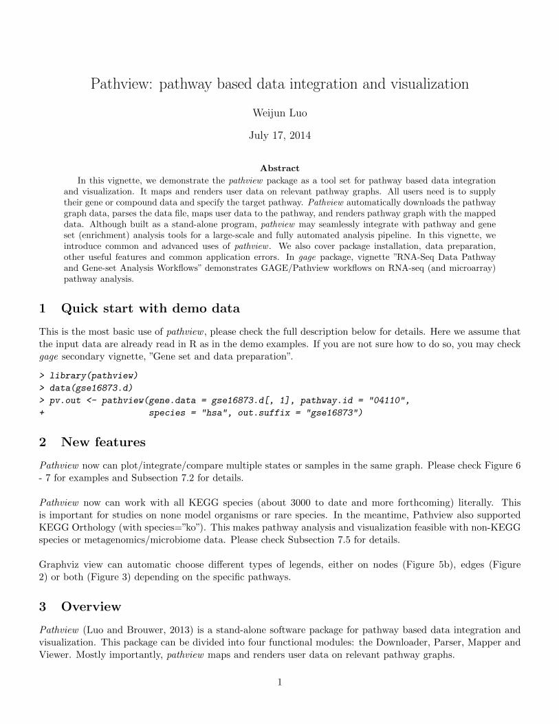
In this vignette, we demonstrate the pathview package as a tool set for pathway based data integrationand visualization. It maps and renders user data on relevant pathway graphs. All users need is to supplytheir gene or compound data and specify the target pathway. Pathview automatically downloads the pathwaygraph data, parses the data file, maps user data to the pathway, and renders pathway graph with the mappeddata. Although built as a stand-alone program, pathview may seamlessly integrate with pathway and geneset (enrichment) analysis tools for a large-scale and fully automated analysis pipeline. In this vignette, weintroduce common and advanced uses of pathview . We also cover package installation, data preparation,other useful features and common application errors. In gage package, vignette ”RNA-Seq Data Pathwayand Gene-set Analysis Workflows” demonstrates GAGE/Pathview workflows on RNA-seq (and microarray)pathway analysis.
1 Quick start with demo data
This is the most basic use of pathview , please check the full description below for details. Here we assume thatthe input data are already read in R as in the demo examples. If you are not sure how to do so, you may checkgage secondary vignette, ”Gene set and data preparation”.
> library(pathview)
> data(gse16873.d)
> pv.out <- pathview(gene.data = gse16873.d[, 1], pathway.id = "04110",
+ species = "hsa", out.suffix = "gse16873")
2 New features
Pathview now can plot/integrate/compare multiple states or samples in the same graph. Please check Figure 6- 7 for examples and Subsection 7.2 for details.
Pathview now can work with all KEGG species (about 3000 to date and more forthcoming) literally. Thisis important for studies on none model organisms or rare species. In the meantime, Pathview also supportedKEGG Orthology (with species=”ko”). This makes pathway analysis and visualization feasible with non-KEGGspecies or metagenomics/microbiome data. Please check Subsection 7.5 for details.
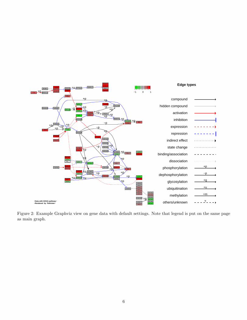
Graphviz view can automatic choose different types of legends, either on nodes (Figure 5b), edges (Figure2) or both (Figure 3) depending on the specific pathways.
3 Overview
Pathview (Luo and Brouwer, 2013) is a stand-alone software package for pathway based data integration andvisualization. This package can be divided into four functional modules: the Downloader, Parser, Mapper andViewer. Mostly importantly, pathview maps and renders user data on relevant pathway graphs.
1
Pathview generates both native KEGG view (like Figure 1 in PNG format) and Graphviz view (like Figure2 in PDF format) for pathways (Section 6). KEGG view keeps all the meta-data on pathways, spacial andtemporal information, tissue/cell types, inputs, outputs and connections. This is important for human readingand interpretation of pathway biology. Graphviz view provides better control of node and edge attributes,better view of pathway topology, better understanding of the pathway analysis statistics. Currently only KEGGpathways are implemented. Hopefully, pathways from Reactome, NCI and other databases will be supportedin the future. Notice that KEGG requires subscription for FTP access since May 2011. However, Pathviewdownloads individual pathway graphs and data files through html access, which is freely available (for academicand non-commerical uses). Pathview uses KEGGgraph (Zhang and Wiemann, 2009) when parsing KEGG xmldata files.
Pathview provides strong support for data integration (Section 7). It works with: 1) essentially all types ofbiological data mappable to pathways, 2) over 10 types of gene or protein IDs, and 20 types of compound ormetabolite IDs, 3) pathways for about 3000 species as well as KEGG orthology, 4) varoius data attributes andformats, i.e. continuous/discrete data, matrices/vectors, single/multiple samples etc.
Pathview is open source, fully automated and error-resistant. Therefore, it seamlessly integrates withpathway or gene set (enrichment) analysis tools. In Section 8, we will show an integrated analysis using pathviewwith anothr the Bioconductor gage package (Luo et al., 2009), available from the Bioconductor website.
Note that although we use microarray data as example gene data in this vignette, Pathview is equallyapplicable to RNA-Seq data and other types of gene/protein centered high throughput data. The secondaryvignette in gage package, ”RNA-Seq Data Pathway and Gene-set Analysis Workflows”, demonstrates suchapplications.
This vignette is written by assuming the user has minimal R/Bioconductor knowledge. Some descriptionsand code chunks cover very basic usage of R. The more experienced users may simply omit these parts.
4 Installation
Assume R and Bioconductor have been correctly installed and accessible under current directory. Otherwise,please contact your system admin or follow the instructions on R website and Bioconductor website. Here Iwould strongly recommend users to install or upgrade to the latest verison of R (3.0.2)/Bioconductor (2.13) forsimpler installation and better use of Pathview . You may need to update your biocLite too if you upgradeR/Biocondutor under Windows.
Start R: from Linux/Unix command line, type R (Enter); for Mac or Windows GUI, double click the Rapplication icon to enter R console.
End R: type in q() when you are finished with the analysis using R, but not now.Two options:Simple way: install with Bioconductor installation script biocLite directly (this included all dependencies
automatically too):
> source("http://bioconductor.org/biocLite.R")
> biocLite("pathview")
Or a bit more complexer: install through R-forge or manually, but require dependence packages to beinstalled using Bioconductor first:
> source("http://bioconductor.org/biocLite.R")
> biocLite(c("Rgraphviz", "png", "KEGGgraph", "org.Hs.eg.db"))
Then install pathview through R-forge.
> install.packages("pathview",repos="http://R-Forge.R-project.org")
Or install manually: download pathview package (from R-forge or Bioconductor, make sure with properversion number and zip format) and save to /your/local/directory/.
2
> install.packages("/your/local/directory/pathview_1.0.0.tar.gz",
+ repos = NULL, type = "source")
Note that there might be problems when installing Rgraphviz or XML (KEGGgraph dependency) packagewith outdated R/Biocondutor. Rgraphviz installation is a bit complicate with R 2.5 (Biocondutor 2.10) orearlier versions. Please check this Readme file on Rgraphviz . On Windows systems,XML frequently needs to beinstalled manually. Its windows binary can be downloaded from CRAN and then:
> install.packages("/your/local/directory/XML_3.95-0.2.zip", repos = NULL)
5 Get Started
Under R, first we load the pathview package:
> library(pathview)
To see a brief overview of the package:
> library(help=pathview)
To get help on any function (say the main function, pathview), use the help command in either one of thefollowing two forms:
> help(pathview)
> ?pathview
6 Common uses for data visualization
Pathview is primarily used for visualizing data on pathway graphs. pathview generates both native KEGGview (like Figure 1) and Graphviz view (like Figure 2). The former render user data on native KEGG pathwaygraphs, hence is natural and more readable for human. The latter layouts pathway graph using Graphviz engine,hence provides better control of node or edge attributes and pathway topology.
We load and look at the demo microarray data first. This is a breast cancer dataset. Here we would like toview the pair-wise gene expression changes between DCIS (disease) and HN (control) samples. Note that themicroarray data are log2 transformed. Hence expression changes are log2 ratios.
> data(gse16873.d)
We also load the demo pathway related data.
> data(demo.paths)
First, we view the exprssion changes of a single sample (pair) on a typical signaling pathway, ”Cell Cycle”,by specifying the gene.data and pathway.id (Figure 1a). The microarray was done on human tissue, hencespecies = "hsa". Note that such native KEGG view was outupt as a raster image in a PNG file in yourworking directory.
> i <- 1
> pv.out <- pathview(gene.data = gse16873.d[, 1], pathway.id = demo.paths$sel.paths[i],
+ species = "hsa", out.suffix = "gse16873", kegg.native = T)
[1] "Downloading xml files for hsa04110, 1/1 pathways.."
[1] "Downloading png files for hsa04110, 1/1 pathways.."
3
> list.files(pattern="hsa04110", full.names=T)
[1] "./hsa04110.gse16873.png" "./hsa04110.png"
[3] "./hsa04110.xml"
> str(pv.out)
List of 2
$ plot.data.gene:'data.frame': 92 obs. of 9 variables:
..$ kegg.names: chr [1:92] "1029" "51343" "4171" "4998" ...
..$ labels : chr [1:92] "CDKN2A" "FZR1" "MCM2" "ORC1" ...
..$ type : chr [1:92] "gene" "gene" "gene" "gene" ...
..$ x : num [1:92] 532 919 553 494 919 919 188 432 123 77 ...
..$ y : num [1:92] 124 536 556 556 297 519 519 191 704 687 ...
..$ width : num [1:92] 46 46 46 46 46 46 46 46 46 46 ...
..$ height : num [1:92] 17 17 17 17 17 17 17 17 17 17 ...
..$ mol.data : num [1:92] 0.129 -0.404 -0.42 0.986 1.181 ...
..$ mol.col : Factor w/ 10 levels "#00FF00","#30EF30",..: 5 3 3 9 9 9 9 9 5 6 ...
$ plot.data.cpd : NULL
> head(pv.out$plot.data.gene)
kegg.names labels type x y width height mol.data mol.col
1 1029 CDKN2A gene 532 124 46 17 0.1291987 #BEBEBE
2 51343 FZR1 gene 919 536 46 17 -0.4043256 #5FDF5F
3 4171 MCM2 gene 553 556 46 17 -0.4202181 #5FDF5F
4 4998 ORC1 gene 494 556 46 17 0.9864873 #FF0000
5 996 CDC27 gene 919 297 46 17 1.1811525 #FF0000
6 996 CDC27 gene 919 519 46 17 1.1811525 #FF0000
Graph from the first example above has a single layer. Node colors were modified on the original graphlayer, and original KEGG node labels (node names) were kept intact. This way the output file size is as smallas the original KEGG PNG file, but the computing time is relative long. If we want a fast view and do notmind doubling the output file size, we may do a two-layer graph with same.layer = F (Figure 1b). This waynode colors and labels are added on an extra layer above the original KEGG graph. Notice that the originalKEGG gene labels (or EC numbers) were replaced by official gene symbols.
> pv.out <- pathview(gene.data = gse16873.d[, 1], pathway.id = demo.paths$sel.paths[i],
+ species = "hsa", out.suffix = "gse16873.2layer", kegg.native = T,
+ same.layer = F)
In the above two examples, we view the data on native KEGG pathway graph. This view we get all notesand meta-data on the KEGG graphs, hence the data is more readable and interpretable. However, the outputgraph is a raster image in PNG format. We may also view the data with a de novo pathway graph layout usingGraphviz engine (Figure 2). The graph has the same set of nodes and edges, but with a different layout. Weget more controls over the nodes and edge attributes and look. Importantly, the graph is a vector image inPDF format in your working directory.
> pv.out <- pathview(gene.data = gse16873.d[, 1], pathway.id = demo.paths$sel.paths[i],
+ species = "hsa", out.suffix = "gse16873", kegg.native = F,
+ sign.pos = demo.paths$spos[i])
> #pv.out remains the same
> dim(pv.out$plot.data.gene)
4

(a)
(b)
Figure 1: Example native KEGG view on gene data with the (a) default settings; or (b) same.layer=F.
5
+p
+p
+p+p
−p
+p +p
+p
+p+p
+p
+p −p
−p−p
−p
−p
+p
+p
+p+p
+p
+p
+p
+p+p
+p
+p
+p
+p
+p
+u
+u+u
+u
+u
SMAD4SMAD2
CDK2CCNE1
CDK7CCNH
CDK2CCNA2
CDK1CCNA2
ORC3ORC5ORC4ORC2ORC1ORC6
MCM7MCM6MCM5MCM4MCM3MCM2
DBF4CDC7
CDK1CCNB1
CDK4CCND1
SKP2SKP1
SKP2SKP1
CDC27CDC20
FZR1CDC27
BUB1BMAD2L1
BUB3
SMC1ASMC3STAG1RAD21
TFDP1E2F4
TFDP1E2F1
RBL1E2F4
TFDP1
CDKN2A
PCNA
PLK1
ATM
BUB1
CDC14B
YWHAB
SFN
CHEK1
CDKN1A
PRKDC
MDM2
CREBBP
PKMYT1
WEE1
PTTG1 ESPL1
RB1
GADD45A
RB1
TP53
CDKN1B
CDKN2BTGFB1
CDC25B
CDC45
CDC6
CDC25A
GSK3B
MAD1L1TTK
CDKN2C
CDKN2D
CDKN2A
MYCZBTB17 ABL1
HDAC1RB1
RBL2
−1 0 1
−Data with KEGG pathway−−Rendered by Pathview−
Edge types
compound
hidden compound
activation
inhibition
expression
repression
indirect effect
state change
binding/association
dissociation
phosphorylation +p
dephosphorylation −p
glycosylation +g
ubiquitination +u
methylation +m
others/unknown ?
Figure 2: Example Graphviz view on gene data with default settings. Note that legend is put on the same pageas main graph.
6
[1] 92 9
> head(pv.out$plot.data.gene)
kegg.names labels type x y width height mol.data mol.col
1 1029 CDKN2A gene 532 124 46 17 0.1291987 #BEBEBE
2 51343 FZR1 gene 919 536 46 17 -0.4043256 #5FDF5F
3 4171 MCM2 gene 553 556 46 17 -0.4202181 #5FDF5F
4 4998 ORC1 gene 494 556 46 17 0.9864873 #FF0000
5 996 CDC27 gene 919 297 46 17 1.1811525 #FF0000
6 996 CDC27 gene 919 519 46 17 1.1811525 #FF0000
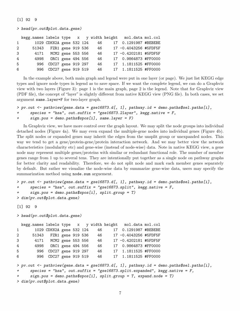
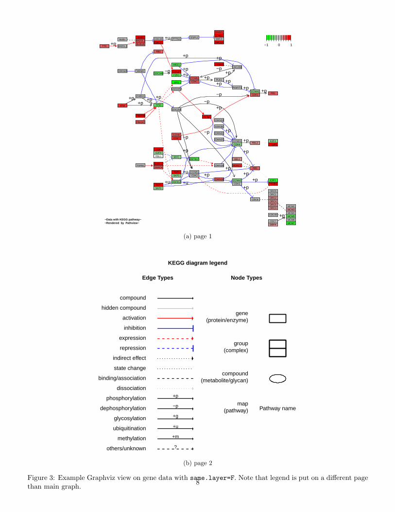
In the example above, both main graph and legend were put in one layer (or page). We just list KEGG edgetypes and ignore node types in legend as to save space. If we want the complete legend, we can do a Graphvizview with two layers (Figure 3): page 1 is the main graph, page 2 is the legend. Note that for Graphviz view(PDF file), the concept of “layer” is slightly different from native KEGG view (PNG file). In both cases, we setargument same.layer=F for two-layer graph.
> pv.out <- pathview(gene.data = gse16873.d[, 1], pathway.id = demo.paths$sel.paths[i],
+ species = "hsa", out.suffix = "gse16873.2layer", kegg.native = F,
+ sign.pos = demo.paths$spos[i], same.layer = F)
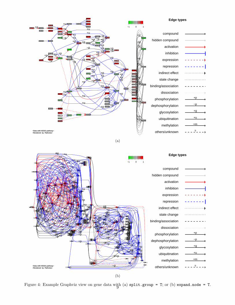
In Graphviz view, we have more control over the graph layout. We may split the node groups into individualdetached nodes (Figure 4a). We may even expand the multiple-gene nodes into individual genes (Figure 4b).The split nodes or expanded genes may inherit the edges from the unsplit group or unexpanded nodes. Thisway we tend to get a gene/protein-gene/protein interaction network. And we may better view the networkcharacteristics (modularity etc) and gene-wise (instead of node-wise) data. Note in native KEGG view, a genenode may represent multiple genes/proteins with similar or redundant functional role. The number of membergenes range from 1 up to several tens. They are intentionally put together as a single node on pathway graphsfor better clarity and readability. Therefore, we do not split node and mark each member genes separatelyby default. But rather we visualize the node-wise data by summarize gene-wise data, users may specify thesummarization method using node.sum arguement.
> pv.out <- pathview(gene.data = gse16873.d[, 1], pathway.id = demo.paths$sel.paths[i],
+ species = "hsa", out.suffix = "gse16873.split", kegg.native = F,
+ sign.pos = demo.paths$spos[i], split.group = T)
> dim(pv.out$plot.data.gene)
[1] 92 9
> head(pv.out$plot.data.gene)
kegg.names labels type x y width height mol.data mol.col
1 1029 CDKN2A gene 532 124 46 17 0.1291987 #BEBEBE
2 51343 FZR1 gene 919 536 46 17 -0.4043256 #5FDF5F
3 4171 MCM2 gene 553 556 46 17 -0.4202181 #5FDF5F
4 4998 ORC1 gene 494 556 46 17 0.9864873 #FF0000
5 996 CDC27 gene 919 297 46 17 1.1811525 #FF0000
6 996 CDC27 gene 919 519 46 17 1.1811525 #FF0000
> pv.out <- pathview(gene.data = gse16873.d[, 1], pathway.id = demo.paths$sel.paths[i],
+ species = "hsa", out.suffix = "gse16873.split.expanded", kegg.native = F,
+ sign.pos = demo.paths$spos[i], split.group = T, expand.node = T)
> dim(pv.out$plot.data.gene)
7
+p
+p
+p+p
−p
+p +p
+p
+p+p
+p
+p −p
−p−p
−p
−p
+p
+p
+p+p
+p
+p
+p
+p+p
+p
+p
+p
+p
+p
+u
+u+u
+u
+u
SMAD4SMAD2
CDK2CCNE1
CDK7CCNH
CDK2CCNA2
CDK1CCNA2
ORC3ORC5ORC4ORC2ORC1ORC6
MCM7MCM6MCM5MCM4MCM3MCM2
DBF4CDC7
CDK1CCNB1
CDK4CCND1
SKP2SKP1
SKP2SKP1
CDC27CDC20
FZR1CDC27
BUB1BMAD2L1
BUB3
SMC1ASMC3STAG1RAD21
TFDP1E2F4
TFDP1E2F1
RBL1E2F4
TFDP1
CDKN2A
PCNA
PLK1
ATM
BUB1
CDC14B
YWHAB
SFN
CHEK1
CDKN1A
PRKDC
MDM2
CREBBP
PKMYT1
WEE1
PTTG1 ESPL1
RB1
GADD45A
RB1
TP53
CDKN1B
CDKN2BTGFB1
CDC25B
CDC45
CDC6
CDC25A
GSK3B
MAD1L1TTK
CDKN2C
CDKN2D
CDKN2A
MYCZBTB17 ABL1
HDAC1RB1
RBL2
−1 0 1
−Data with KEGG pathway−−Rendered by Pathview−
(a) page 1
KEGG diagram legend
compound
hidden compound
activation
inhibition
expression
repression
indirect effect
state change
binding/association
dissociation
phosphorylation +p
dephosphorylation −p
glycosylation +g
ubiquitination +u
methylation +m
others/unknown ?
gene(protein/enzyme)
group(complex)
compound(metabolite/glycan)
map(pathway) Pathway name
Edge Types Node Types
(b) page 2
Figure 3: Example Graphviz view on gene data with same.layer=F. Note that legend is put on a different pagethan main graph.
8
+u
+u
+u
+u
+u
+u+u
+u+u
+p+p
+p
+p
+p
+p
+p
+p
+p
+p
+p
−p
−p
+p +p
+p
+u
+u
+p
+p+p
+p
+u+u
+p
+p
+p
+p
+p
+p
+u
−p
−p
−p−p
−p
+p
+p
+p
+p+p
+p
+p
+p
+p
+p
+p
+p
+p
+p
+p
+p
+p+p
+p
+p
+p
+p
+p
CDKN2A
FZR1
CDC27
CDC27
SKP1
SKP1
ORC6
ORC3
ORC5
ORC4
ORC2
ORC1
MCM7
MCM6
MCM5
MCM4
MCM3
MCM2
CDK1
BUB1B
PCNA
PLK1
ATM
DBF4
MAD2L1
BUB1 BUB3
CDC14BYWHAB
SFN
CHEK1
CDKN1A
PRKDC
MDM2
CREBBP
SKP2
PKMYT1
WEE1
PTTG1 ESPL1 SMC1A
SKP2
RB1
GADD45A
RB1
TP53
CDKN1B
CDKN2B
TGFB1
SMAD4
SMAD2
CDC7
CDC20
CDC25B
CDC45
CDC6
CDC25A
GSK3B
CDK1
CCNB1
CCNA2
CDK7
CDK2
CDK2
CDK4
CCNH
CCNA2
CCNE1
CCND1
MAD1L1TTK
CDKN2C
CDKN2D
CDKN2A
SMC3
STAG1
RAD21
RBL1
E2F4
MYC ZBTB17
ABL1
TFDP1
E2F1
HDAC1
RB1
RBL2TFDP1
E2F4
TFDP1
−1 0 1
−Data with KEGG pathway−−Rendered by Pathview−
Edge types
compound
hidden compound
activation
inhibition
expression
repression
indirect effect
state change
binding/association
dissociation
phosphorylation +p
dephosphorylation −p
glycosylation +g
ubiquitination +u
methylation +m
others/unknown ?
(a)
+u+u+u
+u
+u+u
+u
+u+u
+u
+u+u
+u+u+u
+u
+u+u
+u
+u
+u
+u
+u
+u
+u
+u+u
+u
+u
+u
+u
+u+u
+u
+u+u
+u
+u+u
+u
+u
+u +u
+u
+u
+u
+u
+u
+u
+u+u
+u
+u+u
+u
+u+u
+u
+u+u
+u
+u+u
+u
+u
+u
+u+u
+u
+u
+u+u
+u
+u
+u
+u
+u
+u +u+u+u
+u
+u
+u+u
+u
+u
+u
+u
+u+u
+u+u
+u
+p
+p
+p+p
+p
+p+p+p+p+p+p +p
+p
+p
+p+p+p−p
−p
−p
−p
−p
−p
−p
−p−p
−p
−p−p
−p
−p
−p
−p
−p−p
−p
−p
−p
−p−p−p−p
−p+p
+p
+p+p+p+p
+p
+p
+u
+u+u
+u
+u
+u
+p
+p+p
+p+p
+p
+p+p+p
+u+u
−p−p
−p
−p
−p
−p
+p
+p+p
+p+p
+p
+p+p+p+p
+p +p
+p
+p+p+p
+p
+p
+p
+p
+p
+p+p
+p+p
+p
+p+p
+p
+p
+p
+p+p
+p
+p+p
+p
+p+p
+p
+p+p+p
+p
+p
+p
+p
CDKN2A
FZR1
MCM2MCM3MCM4
MCM5
MCM6
MCM7
ORC6
ORC3
ORC1
ORC2
ORC4
ORC5
ANAPC10
CDC26
ANAPC13
ANAPC2
ANAPC4
ANAPC5
ANAPC7
ANAPC11ANAPC1
CDC23CDC16
CDC27
SKP1
CUL1
RBX1
CDK1
BUB1B
PCNA
PLK1
ATMATR
DBF4
MAD2L2
MAD2L1
BUB1BUB3
CDC14B
CDC14A
YWHAQYWHABYWHAEYWHAG
YWHAHYWHAZ
SFN
CHEK1CHEK2
CDKN1APRKDC
MDM2
CREBBPEP300
SKP2
PKMYT1
WEE2WEE1
PTTG2
PTTG1
ESPL1SMC1BSMC1A
RB1
GADD45GGADD45AGADD45B
TP53
CDKN1B
CDKN1C
CDKN2B
TGFB1TGFB2TGFB3
SMAD4
SMAD2SMAD3
CDC7
CDC20
CDC25B
CDC25C
CDC45
CDC6
CDC25A
GSK3B
CCNB3
CCNB1
CCNB2
CCNA2 CCNA1
CDK7
CDK2
CDK4
CDK6
CCNH
CCNE1
CCNE2
CCND1
CCND2
CCND3
MAD1L1TTK
CDKN2C
CDKN2D
SMC3STAG1STAG2
RAD21
RBL1E2F4
E2F5MYC
ZBTB17
ABL1
TFDP1
TFDP2
E2F1
E2F2E2F3
HDAC1HDAC2
RBL2
−1 0 1
−Data with KEGG pathway−−Rendered by Pathview−
Edge types
compound
hidden compound
activation
inhibition
expression
repression
indirect effect
state change
binding/association
dissociation
phosphorylation +p
dephosphorylation −p
glycosylation +g
ubiquitination +u
methylation +m
others/unknown ?
(b)
Figure 4: Example Graphviz view on gene data with (a) split.group = T; or (b) expand.node = T.9
[1] 124 9
> head(pv.out$plot.data.gene)
kegg.names labels type x y width height mol.data mol.col
hsa:1029 1029 CDKN2A gene 532 124 46 17 0.12919874 #BEBEBE
hsa:51343 51343 FZR1 gene 919 536 46 17 -0.40432563 #5FDF5F
hsa:4171 4171 MCM2 gene 553 556 46 17 0.17968149 #BEBEBE
hsa:4172 4172 MCM3 gene 553 556 46 17 0.33149955 #CE8F8F
hsa:4173 4173 MCM4 gene 553 556 46 17 0.06996779 #BEBEBE
hsa:4174 4174 MCM5 gene 553 556 46 17 -0.42874682 #5FDF5F
7 Data integration
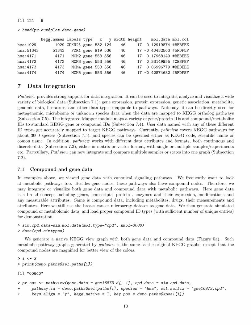
Pathview provides strong support for data integration. It can be used to integrate, analyze and visualize a widevariety of biological data (Subsection 7.1): gene expression, protein expression, genetic association, metabolite,genomic data, literature, and other data types mappable to pathways. Notebaly, it can be directly used formetagenomic, microbiome or unknown species data when the data are mapped to KEGG ortholog pathways(Subsection 7.5). The integrated Mapper module maps a variety of gene/protein IDs and compound/metaboliteIDs to standard KEGG gene or compound IDs (Subsection 7.4). User data named with any of these differentID types get accurately mapped to target KEGG pathways. Currently, pathview covers KEGG pathways forabout 3000 species (Subsection 7.5), and species can be specified either as KEGG code, scientific name orcomon name. In addition, pathview works with different data attributes and formats, both continuous anddiscrete data (Subsection 7.3), either in matrix or vector format, with single or multiple samples/experimentsetc. Partcullary, Pathview can now integrate and compare multiple samples or states into one graph (Subsection7.2).
7.1 Compound and gene data
In examples above, we viewed gene data with canonical signaling pathways. We frequently want to lookat metabolic pathways too. Besides gene nodes, these pathways also have compound nodes. Therefore, wemay integrate or visualize both gene data and compound data with metabolic pathways. Here gene datais a broad concept including genes, transcripts, protein , enzymes and their expression, modifications andany measurable attributes. Same is compound data, including metabolites, drugs, their measurements andattributes. Here we still use the breast cancer microarray dataset as gene data. We then generate simulatedcompound or metabolomic data, and load proper compound ID types (with sufficient number of unique entries)for demonstration.
> sim.cpd.data=sim.mol.data(mol.type="cpd", nmol=3000)
> data(cpd.simtypes)
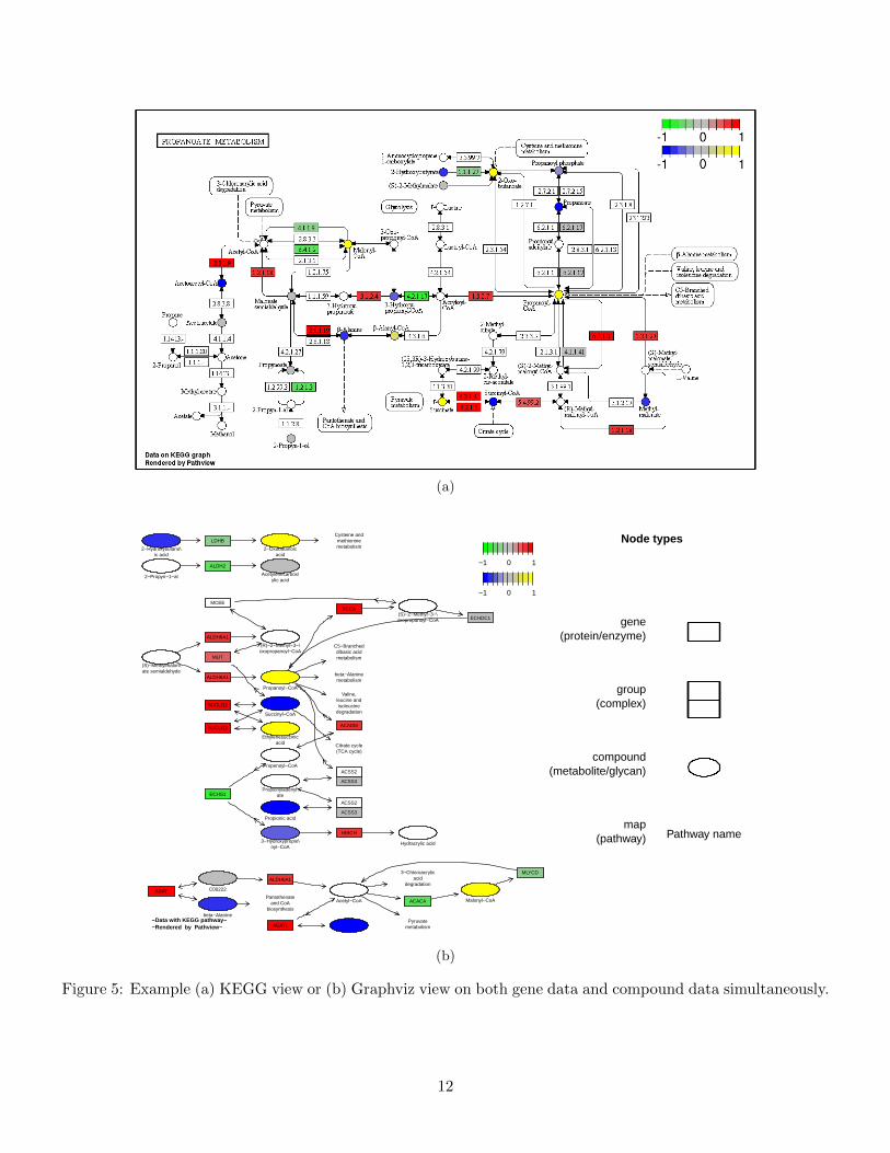
We generate a native KEGG view graph with both gene data and compound data (Figure 5a). Suchmetabolic pathway graphs generated by pathview is the same as the original KEGG graphs, except that thecompound nodes are magnified for better view of the colors.
> i <- 3
> print(demo.paths$sel.paths[i])
[1] "00640"
> pv.out <- pathview(gene.data = gse16873.d[, 1], cpd.data = sim.cpd.data,
+ pathway.id = demo.paths$sel.paths[i], species = "hsa", out.suffix = "gse16873.cpd",
+ keys.align = "y", kegg.native = T, key.pos = demo.paths$kpos1[i])
10
[1] "Downloading xml files for hsa00640, 1/1 pathways.."
[1] "Downloading png files for hsa00640, 1/1 pathways.."
> str(pv.out)
List of 2
$ plot.data.gene:'data.frame': 22 obs. of 9 variables:
..$ kegg.names: chr [1:22] "4329" "4329" "84693" "5095" ...
..$ labels : chr [1:22] "ALDH6A1" "ALDH6A1" "MCEE" "PCCA" ...
..$ type : chr [1:22] "gene" "gene" "gene" "gene" ...
..$ x : num [1:22] 970 924 807 886 833 830 830 780 780 747 ...
..$ y : num [1:22] 430 609 526 430 460 309 223 309 223 556 ...
..$ width : num [1:22] 46 46 46 46 46 46 46 46 46 46 ...
..$ height : num [1:22] 17 17 17 17 17 17 17 17 17 17 ...
..$ mol.data : num [1:22] 0.747 0.747 NA 1.19 0.162 ...
..$ mol.col : Factor w/ 8 levels "#30EF30","#5FDF5F",..: 6 6 8 7 4 4 4 8 8 5 ...
$ plot.data.cpd :'data.frame': 40 obs. of 9 variables:
..$ kegg.names: chr [1:40] "C04225" "C02614" "C00109" "C02876" ...
..$ labels : chr [1:40] "C04225" "C02614" "C00109" "C02876" ...
..$ type : chr [1:40] "compound" "compound" "compound" "compound" ...
..$ x : num [1:40] 680 585 680 805 805 585 579 579 579 805 ...
..$ y : num [1:40] 495 143 118 115 184 90 184 255 354 351 ...
..$ width : num [1:40] 8 8 8 8 8 8 8 8 8 8 ...
..$ height : num [1:40] 8 8 8 8 8 8 8 8 8 8 ...
..$ mol.data : num [1:40] NA 0.000376 0.825575 -0.35501 -1.551161 ...
..$ mol.col : Factor w/ 8 levels "#0000FF","#3030EF",..: 8 5 7 4 1 8 8 8 8 7 ...
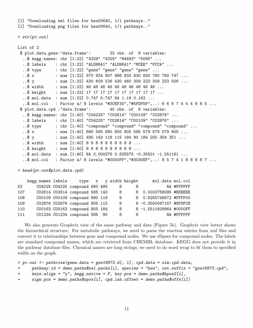
> head(pv.out$plot.data.cpd)
kegg.names labels type x y width height mol.data mol.col
53 C04225 C04225 compound 680 495 8 8 NA #FFFFFF
107 C02614 C02614 compound 585 143 8 8 0.0003758095 #BEBEBE
108 C00109 C00109 compound 680 118 8 8 0.8255746672 #FFFF00
109 C02876 C02876 compound 805 115 8 8 -0.3550097157 #8F8FCE
110 C00163 C00163 compound 805 184 8 8 -1.5511608864 #0000FF
111 C01234 C01234 compound 585 90 8 8 NA #FFFFFF
We also generate Graphviz view of the same pathway and data (Figure 5b). Graphviz view better showsthe hierarchical structure. For metabolic pathways, we need to parse the reaction entries from xml files andconvert it to relationships between gene and compound nodes. We use ellipses for compound nodes. The labelsare standard compound names, which are retrieved from CHEMBL database. KEGG does not provide it inthe pathway database files. Chemical names are long strings, we need to do word wrap to fit them to specifiedwidth on the graph.
> pv.out <- pathview(gene.data = gse16873.d[, 1], cpd.data = sim.cpd.data,
+ pathway.id = demo.paths$sel.paths[i], species = "hsa", out.suffix = "gse16873.cpd",
+ keys.align = "y", kegg.native = F, key.pos = demo.paths$kpos2[i],
+ sign.pos = demo.paths$spos[i], cpd.lab.offset = demo.paths$offs[i])
11
(a)
ACSS3
ACSS2
ACSS3
ACSS2
3−Chloroacrylicacid
degradation
ALDH6A1
ALDH6A1
MCEEPCCA
ECHDC1
MUT
SUCLG2
SUCLG2
HIBCH
ABAT
ALDH2
ALDH6A1
ACAT1
ACACA
MLYCD
LDHB
Pyruvatemetabolism
Citrate cycle(TCA cycle)
Valine,leucine andisoleucine
degradation
C5−Brancheddibasic acidmetabolism
Pantothenateand CoA
biosynthesis
beta−Alaninemetabolism
ECHS1
Cysteine andmethioninemetabolism
ACADM
2−Oxobutanoicacid
Propionic acid
Propenoyl−CoA
Propanoyl−CoA
(S)−2−Methyl−3−\oxopropanoyl−CoA
Succinyl−CoA
Ethylenesuccinicacid
Acetoacetyl−CoA
C00222
Acetylenecarbox\ylic acid
Acetyl−CoA
Hydracrylic acid
beta−Alanine
3−Hydroxypropio\nyl−CoA
Malonyl−CoA
2−Hydroxybutano\ic acid
2−Propyn−1−al
Propionyladenyl\ate
(S)−Methylmalon\ate semialdehyde
(R)−2−Methyl−3−\oxopropanoyl−CoA
−1 0 1
−1 0 1
−Data with KEGG pathway−−Rendered by Pathview−
Node types
gene(protein/enzyme)
group(complex)
compound(metabolite/glycan)
map(pathway) Pathway name
(b)
Figure 5: Example (a) KEGG view or (b) Graphviz view on both gene data and compound data simultaneously.
12
7.2 Multiple states or samples
In all previous examples, we looked at single sample data, which are either vector or single-column matrix.Pathview also handles multiple sample data, it used to generate graph for each sample. Since version 1.1.6,Pathview can integrate and plot multiple samples or states into one graph (Figure 6 - 7).
Let’s simulate compound data with multiple replicate samples first.
> set.seed(10)
> sim.cpd.data2 = matrix(sample(sim.cpd.data, 18000,
+ replace = T), ncol = 6)
> rownames(sim.cpd.data2) = names(sim.cpd.data)
> colnames(sim.cpd.data2) = paste("exp", 1:6, sep = "")
> head(sim.cpd.data2, 3)
exp1 exp2 exp3 exp4 exp5 exp6
C02787 0.62355826 -0.1108793 1.069398 -0.9595403 1.653444849 1.360614
C08521 -1.23737070 0.4676360 -2.064253 -0.6593838 0.004274093 0.512765
C01043 -0.01768295 0.5472769 -0.592388 -0.1190882 0.950917578 -1.130288
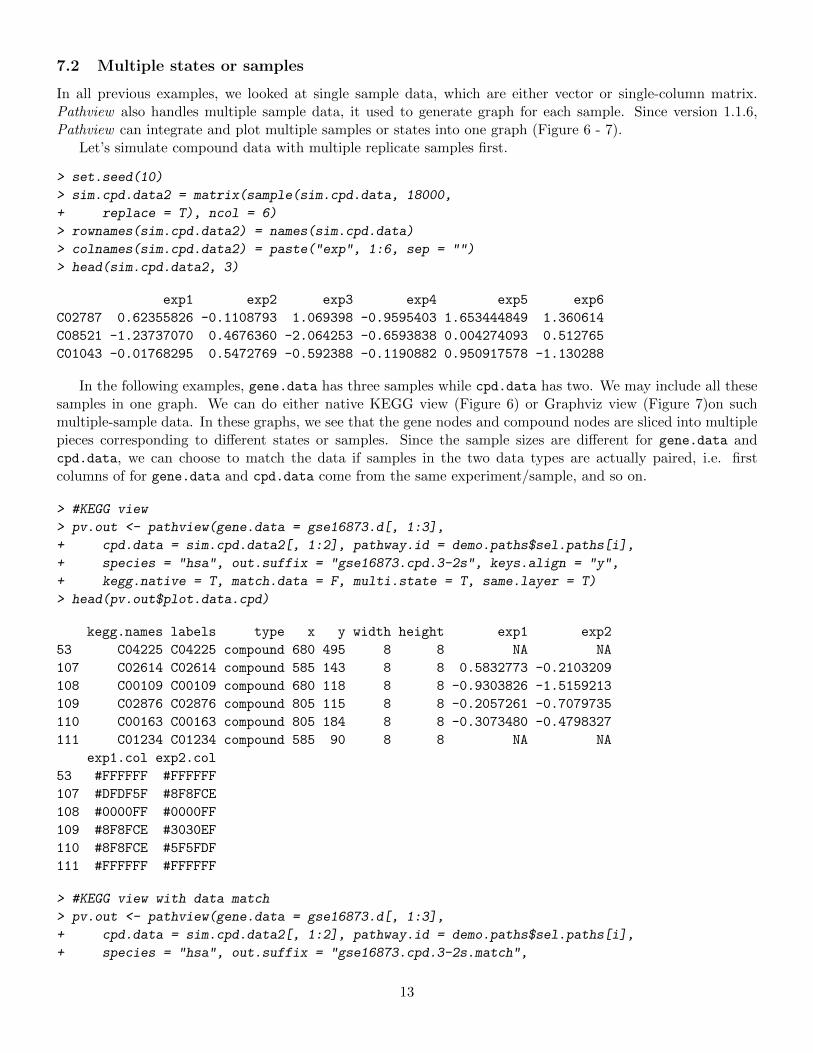
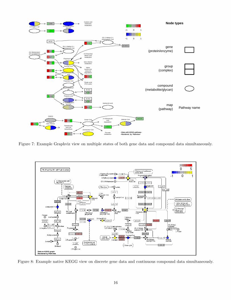
In the following examples, gene.data has three samples while cpd.data has two. We may include all thesesamples in one graph. We can do either native KEGG view (Figure 6) or Graphviz view (Figure 7)on suchmultiple-sample data. In these graphs, we see that the gene nodes and compound nodes are sliced into multiplepieces corresponding to different states or samples. Since the sample sizes are different for gene.data andcpd.data, we can choose to match the data if samples in the two data types are actually paired, i.e. firstcolumns of for gene.data and cpd.data come from the same experiment/sample, and so on.
> #KEGG view
> pv.out <- pathview(gene.data = gse16873.d[, 1:3],
+ cpd.data = sim.cpd.data2[, 1:2], pathway.id = demo.paths$sel.paths[i],
+ species = "hsa", out.suffix = "gse16873.cpd.3-2s", keys.align = "y",
+ kegg.native = T, match.data = F, multi.state = T, same.layer = T)
> head(pv.out$plot.data.cpd)
kegg.names labels type x y width height exp1 exp2
53 C04225 C04225 compound 680 495 8 8 NA NA
107 C02614 C02614 compound 585 143 8 8 0.5832773 -0.2103209
108 C00109 C00109 compound 680 118 8 8 -0.9303826 -1.5159213
109 C02876 C02876 compound 805 115 8 8 -0.2057261 -0.7079735
110 C00163 C00163 compound 805 184 8 8 -0.3073480 -0.4798327
111 C01234 C01234 compound 585 90 8 8 NA NA
exp1.col exp2.col
53 #FFFFFF #FFFFFF
107 #DFDF5F #8F8FCE
108 #0000FF #0000FF
109 #8F8FCE #3030EF
110 #8F8FCE #5F5FDF
111 #FFFFFF #FFFFFF
> #KEGG view with data match
> pv.out <- pathview(gene.data = gse16873.d[, 1:3],
+ cpd.data = sim.cpd.data2[, 1:2], pathway.id = demo.paths$sel.paths[i],
+ species = "hsa", out.suffix = "gse16873.cpd.3-2s.match",
13
+ keys.align = "y", kegg.native = T, match.data = T, multi.state = T,
+ same.layer = T)
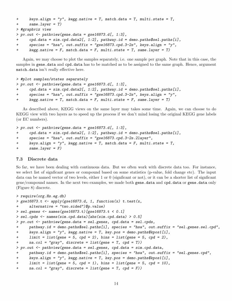
> #graphviz view
> pv.out <- pathview(gene.data = gse16873.d[, 1:3],
+ cpd.data = sim.cpd.data2[, 1:2], pathway.id = demo.paths$sel.paths[i],
+ species = "hsa", out.suffix = "gse16873.cpd.3-2s", keys.align = "y",
+ kegg.native = F, match.data = F, multi.state = T, same.layer = T)
Again, we may choose to plot the samples separately, i.e. one sample per graph. Note that in this case, thesamples in gene.data and cpd.data has to be matched as to be assigned to the same graph. Hence, argumentmatch.data isn’t really effective here.
> #plot samples/states separately
> pv.out <- pathview(gene.data = gse16873.d[, 1:3],
+ cpd.data = sim.cpd.data2[, 1:2], pathway.id = demo.paths$sel.paths[i],
+ species = "hsa", out.suffix = "gse16873.cpd.3-2s", keys.align = "y",
+ kegg.native = T, match.data = F, multi.state = F, same.layer = T)
As described above, KEGG views on the same layer may takes some time. Again, we can choose to doKEGG view with two layers as to speed up the process if we don’t mind losing the original KEGG gene labels(or EC numbers).
> pv.out <- pathview(gene.data = gse16873.d[, 1:3],
+ cpd.data = sim.cpd.data2[, 1:2], pathway.id = demo.paths$sel.paths[i],
+ species = "hsa", out.suffix = "gse16873.cpd.3-2s.2layer",
+ keys.align = "y", kegg.native = T, match.data = F, multi.state = T,
+ same.layer = F)
7.3 Discrete data
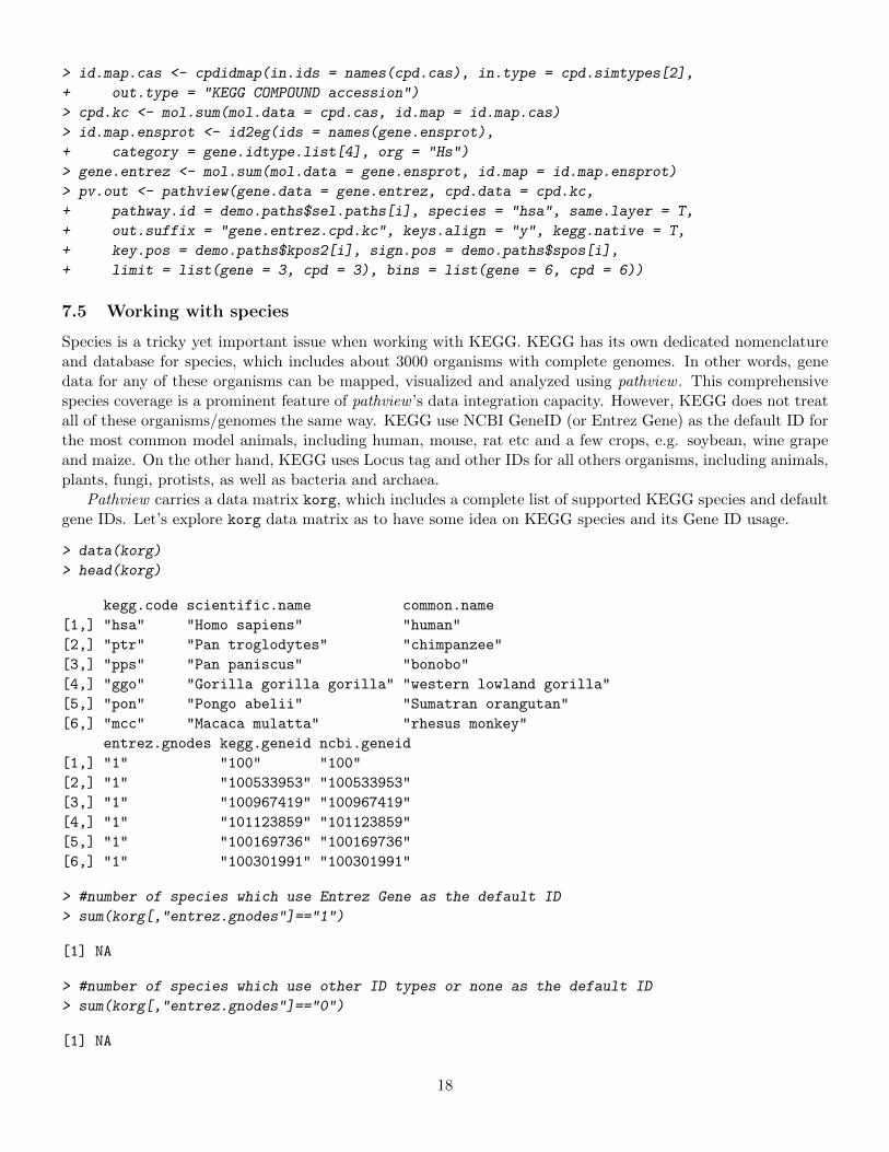
So far, we have been dealing with continuous data. But we often work with discrete data too. For instance,we select list of signficant genes or compound based on some statistics (p-value, fold change etc). The inputdata can be named vector of two levels, either 1 or 0 (signficant or not), or it can be a shorter list of signficantgene/compound names. In the next two examples, we made both gene.data and cpd.data or gene.data only(Figure 8) discrete.
> require(org.Hs.eg.db)
> gse16873.t <- apply(gse16873.d, 1, function(x) t.test(x,
+ alternative = "two.sided")$p.value)
> sel.genes <- names(gse16873.t)[gse16873.t < 0.1]
> sel.cpds <- names(sim.cpd.data)[abs(sim.cpd.data) > 0.5]
> pv.out <- pathview(gene.data = sel.genes, cpd.data = sel.cpds,
+ pathway.id = demo.paths$sel.paths[i], species = "hsa", out.suffix = "sel.genes.sel.cpd",
+ keys.align = "y", kegg.native = T, key.pos = demo.paths$kpos1[i],
+ limit = list(gene = 5, cpd = 2), bins = list(gene = 5, cpd = 2),
+ na.col = "gray", discrete = list(gene = T, cpd = T))
> pv.out <- pathview(gene.data = sel.genes, cpd.data = sim.cpd.data,
+ pathway.id = demo.paths$sel.paths[i], species = "hsa", out.suffix = "sel.genes.cpd",
+ keys.align = "y", kegg.native = T, key.pos = demo.paths$kpos1[i],
+ limit = list(gene = 5, cpd = 1), bins = list(gene = 5, cpd = 10),
+ na.col = "gray", discrete = list(gene = T, cpd = F))
14
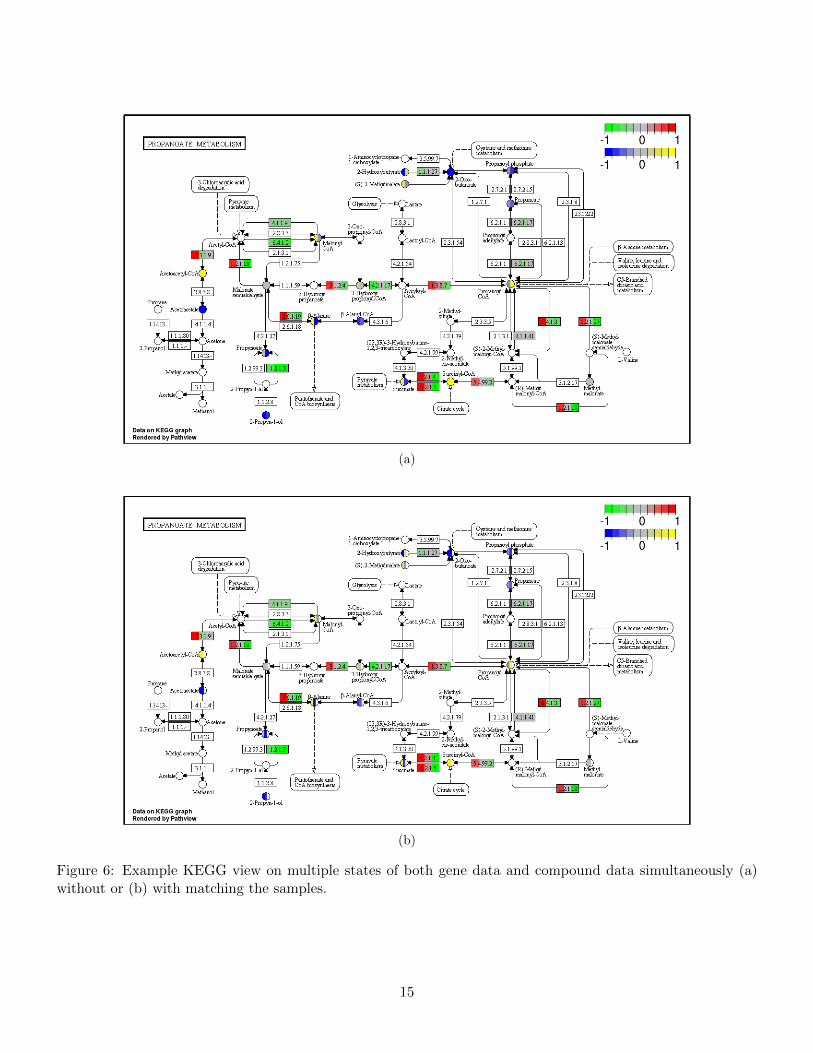
(a)
(b)
Figure 6: Example KEGG view on multiple states of both gene data and compound data simultaneously (a)without or (b) with matching the samples.
15
ACSS3
ACSS2
ACSS3
ACSS2
3−Chloroacrylicacid
degradation
ALDH6A1
ALDH6A1
MCEEPCCA
ECHDC1
MUT
SUCLG2
SUCLG2
HIBCH
ABAT
ALDH2
ALDH6A1
ACAT1
ACACA
MLYCD
LDHB
Pyruvatemetabolism
Citrate cycle(TCA cycle)
Valine,leucine andisoleucine
degradation
C5−Brancheddibasic acidmetabolism
Pantothenateand CoA
biosynthesis
beta−Alaninemetabolism
ECHS1
Cysteine andmethioninemetabolism
ACADM
acid
Propionic acid
Propenoyl−CoA
Propanoyl−CoA
(S)−2−Methyl−3−\oxopropanoyl−CoA
Succinyl−CoA
Ethylenesuccinicacid
Acetoacetyl−CoA
C00222
Acetylenecarbox\ylic acid
Acetyl−CoA
Hydracrylic acid
beta−Alanine
3−Hydroxypropio\nyl−CoA
Malonyl−CoA
ic acid
2−Propyn−1−al
Propionyladenyl\ate
(S)−Methylmalon\ate semialdehyde
(R)−2−Methyl−3−\oxopropanoyl−CoA
−1 0 1
−1 0 1
−Data with KEGG pathway−−Rendered by Pathview−
Node types
gene(protein/enzyme)
group(complex)
compound(metabolite/glycan)
map(pathway) Pathway name
Figure 7: Example Graphviz view on multiple states of both gene data and compound data simultaneously.
Figure 8: Example native KEGG view on discrete gene data and continuous compound data simultaneously.
16

Figure 9: Example native KEGG view on gene data and compound data with other ID types.
7.4 ID mapping
A distinguished feature of pathview is its strong ID mapping capability. The integrated Mapper module mapsover 10 types of gene or protein IDs, and 20 types of compound or metabolite IDs to standard KEGG gene orcompound IDs, and also maps between these external IDs. In other words, user data named with any of thesedifferent ID types get accurately mapped to target KEGG pathways. Pathview applies to pathways for about3000 species, and species can be specified in multiple formats: KEGG code, scientific name or comon name.
The following example makes use of the integrated mapper to map external ID types to standard KEGG IDsautomatically (Figure 9). We only need to specify the external ID types using gene.idtype and cpd.idtype
arguments. Note that automatic mapping is limited to certain ID types. For details check: gene.idtype.listand data(rn.list); names(rn.list).
> cpd.cas <- sim.mol.data(mol.type = "cpd", id.type = cpd.simtypes[2],
+ nmol = 10000)
> gene.ensprot <- sim.mol.data(mol.type = "gene", id.type = gene.idtype.list[4],
+ nmol = 50000)
> pv.out <- pathview(gene.data = gene.ensprot, cpd.data = cpd.cas,
+ gene.idtype = gene.idtype.list[4], cpd.idtype = cpd.simtypes[2],
+ pathway.id = demo.paths$sel.paths[i], species = "hsa", same.layer = T,
+ out.suffix = "gene.ensprot.cpd.cas", keys.align = "y", kegg.native = T,
+ key.pos = demo.paths$kpos2[i], sign.pos = demo.paths$spos[i],
+ limit = list(gene = 3, cpd = 3), bins = list(gene = 6, cpd = 6))
For external IDs not in the auto-mapping lists, we may make use of the mol.sum function (also part of theMapper module) to do the ID and data mapping explicitly. Here we need to provide id.map, the mapping matrixbetween external ID and KEGG standard ID. We use ID mapping functions including id2eg and cpdidmap
etc to get id.map matrix. Note that these ID mapping functions can be used independent of pathview mainfunction. The following example use this route with the simulated gene.ensprot and cpd.kc data above, andwe get the same results (Figure not shown).
17
> id.map.cas <- cpdidmap(in.ids = names(cpd.cas), in.type = cpd.simtypes[2],
+ out.type = "KEGG COMPOUND accession")
> cpd.kc <- mol.sum(mol.data = cpd.cas, id.map = id.map.cas)
> id.map.ensprot <- id2eg(ids = names(gene.ensprot),
+ category = gene.idtype.list[4], org = "Hs")
> gene.entrez <- mol.sum(mol.data = gene.ensprot, id.map = id.map.ensprot)
> pv.out <- pathview(gene.data = gene.entrez, cpd.data = cpd.kc,
+ pathway.id = demo.paths$sel.paths[i], species = "hsa", same.layer = T,
+ out.suffix = "gene.entrez.cpd.kc", keys.align = "y", kegg.native = T,
+ key.pos = demo.paths$kpos2[i], sign.pos = demo.paths$spos[i],
+ limit = list(gene = 3, cpd = 3), bins = list(gene = 6, cpd = 6))
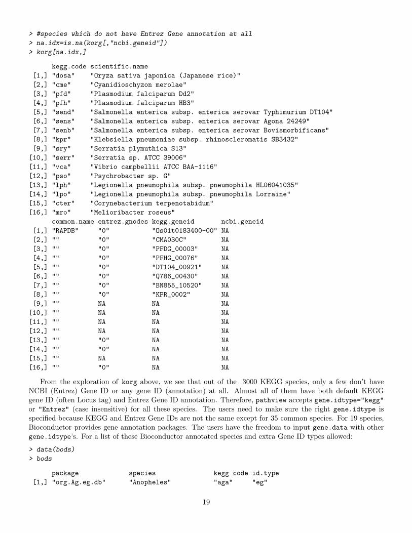
7.5 Working with species
Species is a tricky yet important issue when working with KEGG. KEGG has its own dedicated nomenclatureand database for species, which includes about 3000 organisms with complete genomes. In other words, genedata for any of these organisms can be mapped, visualized and analyzed using pathview . This comprehensivespecies coverage is a prominent feature of pathview ’s data integration capacity. However, KEGG does not treatall of these organisms/genomes the same way. KEGG use NCBI GeneID (or Entrez Gene) as the default ID forthe most common model animals, including human, mouse, rat etc and a few crops, e.g. soybean, wine grapeand maize. On the other hand, KEGG uses Locus tag and other IDs for all others organisms, including animals,plants, fungi, protists, as well as bacteria and archaea.
Pathview carries a data matrix korg, which includes a complete list of supported KEGG species and defaultgene IDs. Let’s explore korg data matrix as to have some idea on KEGG species and its Gene ID usage.
> data(korg)
> head(korg)
kegg.code scientific.name common.name
[1,] "hsa" "Homo sapiens" "human"
[2,] "ptr" "Pan troglodytes" "chimpanzee"
[3,] "pps" "Pan paniscus" "bonobo"
[4,] "ggo" "Gorilla gorilla gorilla" "western lowland gorilla"
[5,] "pon" "Pongo abelii" "Sumatran orangutan"
[6,] "mcc" "Macaca mulatta" "rhesus monkey"
entrez.gnodes kegg.geneid ncbi.geneid
[1,] "1" "100" "100"
[2,] "1" "100533953" "100533953"
[3,] "1" "100967419" "100967419"
[4,] "1" "101123859" "101123859"
[5,] "1" "100169736" "100169736"
[6,] "1" "100301991" "100301991"
> #number of species which use Entrez Gene as the default ID
> sum(korg[,"entrez.gnodes"]=="1")
[1] NA
> #number of species which use other ID types or none as the default ID
> sum(korg[,"entrez.gnodes"]=="0")
[1] NA
18
> #species which do not have Entrez Gene annotation at all
> na.idx=is.na(korg[,"ncbi.geneid"])
> korg[na.idx,]
kegg.code scientific.name
[1,] "dosa" "Oryza sativa japonica (Japanese rice)"
[2,] "cme" "Cyanidioschyzon merolae"
[3,] "pfd" "Plasmodium falciparum Dd2"
[4,] "pfh" "Plasmodium falciparum HB3"
[5,] "send" "Salmonella enterica subsp. enterica serovar Typhimurium DT104"
[6,] "sens" "Salmonella enterica subsp. enterica serovar Agona 24249"
[7,] "senb" "Salmonella enterica subsp. enterica serovar Bovismorbificans"
[8,] "kpr" "Klebsiella pneumoniae subsp. rhinoscleromatis SB3432"
[9,] "sry" "Serratia plymuthica S13"
[10,] "serr" "Serratia sp. ATCC 39006"
[11,] "vca" "Vibrio campbellii ATCC BAA-1116"
[12,] "pso" "Psychrobacter sp. G"
[13,] "lph" "Legionella pneumophila subsp. pneumophila HL06041035"
[14,] "lpo" "Legionella pneumophila subsp. pneumophila Lorraine"
[15,] "cter" "Corynebacterium terpenotabidum"
[16,] "mro" "Melioribacter roseus"
common.name entrez.gnodes kegg.geneid ncbi.geneid
[1,] "RAPDB" "0" "Os01t0183400-00" NA
[2,] "" "0" "CMA030C" NA
[3,] "" "0" "PFDG_00003" NA
[4,] "" "0" "PFHG_00076" NA
[5,] "" "0" "DT104_00921" NA
[6,] "" "0" "Q786_00430" NA
[7,] "" "0" "BN855_10520" NA
[8,] "" "0" "KPR_0002" NA
[9,] "" NA NA NA
[10,] "" NA NA NA
[11,] "" NA NA NA
[12,] "" NA NA NA
[13,] "" "0" NA NA
[14,] "" "0" NA NA
[15,] "" NA NA NA
[16,] "" "0" NA NA
From the exploration of korg above, we see that out of the 3000 KEGG species, only a few don’t haveNCBI (Entrez) Gene ID or any gene ID (annotation) at all. Almost all of them have both default KEGGgene ID (often Locus tag) and Entrez Gene ID annotation. Therefore, pathview accepts gene.idtype="kegg"or "Entrez" (case insensitive) for all these species. The users need to make sure the right gene.idtype isspecified because KEGG and Entrez Gene IDs are not the same except for 35 common species. For 19 species,Bioconductor provides gene annotation packages. The users have the freedom to input gene.data with othergene.idtype’s. For a list of these Bioconductor annotated species and extra Gene ID types allowed:
> data(bods)
> bods
package species kegg code id.type
[1,] "org.Ag.eg.db" "Anopheles" "aga" "eg"
19
[2,] "org.At.tair.db" "Arabidopsis" "ath" "tair"
[3,] "org.Bt.eg.db" "Bovine" "bta" "eg"
[4,] "org.Ce.eg.db" "Worm" "cel" "eg"
[5,] "org.Cf.eg.db" "Canine" "cfa" "eg"
[6,] "org.Dm.eg.db" "Fly" "dme" "eg"
[7,] "org.Dr.eg.db" "Zebrafish" "dre" "eg"
[8,] "org.EcK12.eg.db" "E coli strain K12" "eco" "eg"
[9,] "org.EcSakai.eg.db" "E coli strain Sakai" "ecs" "eg"
[10,] "org.Gg.eg.db" "Chicken" "gga" "eg"
[11,] "org.Hs.eg.db" "Human" "hsa" "eg"
[12,] "org.Mm.eg.db" "Mouse" "mmu" "eg"
[13,] "org.Mmu.eg.db" "Rhesus" "mcc" "eg"
[14,] "org.Pf.plasmo.db" "Malaria" "pfa" "orf"
[15,] "org.Pt.eg.db" "Chimp" "ptr" "eg"
[16,] "org.Rn.eg.db" "Rat" "rno" "eg"
[17,] "org.Sc.sgd.db" "Yeast" "sce" "orf"
[18,] "org.Ss.eg.db" "Pig" "ssc" "eg"
[19,] "org.Xl.eg.db" "Xenopus" "xla" "eg"
> data(gene.idtype.list)
> gene.idtype.list
[1] "SYMBOL" "GENENAME" "ENSEMBL" "ENSEMBLPROT" "PROSITE"
[6] "UNIGENE" "UNIPROT" "ACCNUM" "ENSEMBLTRANS" "REFSEQ"
All previous examples show human data, where Entrez Gene is KEGG’s default gene ID. Pathview now(since version 1.1.5) explicitly handles species which use Locus tag or other gene IDs as the KEGG default ID.Below are an couple of examples with E coli strain K12 data. First, we work on gene data with the defaultKEGG ID (Locus tag) for E coli K12.
> eco.dat.kegg <- sim.mol.data(mol.type="gene",id.type="kegg",species="eco",nmol=3000)
> head(eco.dat.kegg)
b1447 b1206 b2579 b0264 b2197 b2267
-1.15259948 0.46416071 0.72893247 0.41061745 -1.46114720 -0.01890809
> pv.out <- pathview(gene.data = eco.dat.kegg, gene.idtype="kegg",
+ pathway.id = "00640", species = "eco", out.suffix = "eco.kegg",
+ kegg.native = T, same.layer=T)
[1] "Downloading xml files for eco00640, 1/1 pathways.."
[1] "Downloading png files for eco00640, 1/1 pathways.."
We may also work on gene data with Entrez Gene ID for E coli K12 the same way as for human.
> eco.dat.entrez <- sim.mol.data(mol.type="gene",id.type="entrez",species="eco",nmol=3000)
> head(eco.dat.entrez)
946008 945770 947068 947698 946697 946750
-1.15259948 0.46416071 0.72893247 0.41061745 -1.46114720 -0.01890809
> pv.out <- pathview(gene.data = eco.dat.entrez, gene.idtype="entrez",
+ pathway.id = "00640", species = "eco", out.suffix = "eco.entrez",
+ kegg.native = T, same.layer=T)
20
Based on the bods data described above, E coli K12 is an Bioconductor annotated species. Hence we mayfurther work on its gene data with other ID types, for example, official gene symbols. When calling pathview,such data need to be mapped to Entrez Gene ID first (if not yet), then to default KEGG ID (Locus tag).Therefore, it takes longer time than the last example.
> egid.eco=eg2id(names(eco.dat.entrez), category="symbol", pkg="org.EcK12.eg.db")
> eco.dat.symbol <- eco.dat.entrez
> names(eco.dat.symbol) <- egid.eco[,2]
> head(eco.dat.kegg)
> pv.out <- pathview(gene.data = eco.dat.symbol, gene.idtype="symbol",
+ pathway.id = "00640", species = "eco", out.suffix = "eco.symbol.2layer",
+ kegg.native = T, same.layer=F)
Importantly, pathview can be directly used for metagenomic or microbiome data when the data are mappedto KEGG ortholog pathways. And data from any new species that has not been annotated and includedin KEGG (non-KEGG species) can also been analyzed and visualized using pathview by mapping to KEGGortholog pathways the same way. In the next example, we simulate the mapped KEGG ortholog gene data first.Then the data is input as gene.data with species="ko". Check pathview function for details.
> ko.data=sim.mol.data(mol.type="gene.ko", nmol=5000)
> pv.out <- pathview(gene.data = ko.data, pathway.id = "04112",
+ species = "ko", out.suffix = "ko.data", kegg.native = T)
[1] "Downloading xml files for ko04112, 1/1 pathways.."
[1] "Downloading png files for ko04112, 1/1 pathways.."
8 Integrated workflow with pathway analysis
Although built as a stand alone program, Pathview may seamlessly integrate with pathway and functionalanalysis tools for large-scale and fully automated analysis pipeline. The next example shows how to connectcommon pathway analysis to results rendering with pathview . The pathway analysis was done using anotherBioconductor package gage (Luo et al., 2009), and the selected signficant pathways plus the expression data werethen piped to pathview for auomated results visualization (Figure not shown). In gage package, vignette ”RNA-Seq Data Pathway and Gene-set Analysis Workflows” demonstrates GAGE/Pathview workflows on RNA-seq(and microarray) pathway analysis.
> library(gage)
> data(gse16873)
> cn <- colnames(gse16873)
> hn <- grep('HN',cn, ignore.case =TRUE)
> dcis <- grep('DCIS',cn, ignore.case =TRUE)
> kgs.file <- system.file("extdata", "kegg.sigmet.rda", package = "pathview")
> data(kegg.gs)
> gse16873.kegg.p <- gage(gse16873, gsets = kegg.gs,
+ ref = hn, samp = dcis)
> gse16873.d <- gagePrep(gse16873, ref = hn, samp = dcis)
> sel <- gse16873.kegg.p$greater[, "q.val"] < 0.1 & !is.na(gse16873.kegg.p$greater[,
+ "q.val"])
> path.ids <- rownames(gse16873.kegg.p$greater)[sel]
> path.ids2 <- substr(path.ids[c(1, 2, 7)], 1, 8)
> pv.out.list <- sapply(path.ids2, function(pid) pathview(gene.data = gse16873.d[,
+ 1:2], pathway.id = pid, species = "hsa"))
21
9 Common Errors
� mismatch between the IDs for gene.data (or cpd.data) and gene.idtype (or cpd.idtype). For example,gene.data or cpd.data uses some extern ID types, while gene.idtype = "entrez" and cpd.idtype =
"kegg" (default).
� mismatch between gene.data (or cpd.data) and species. For example, gene.data come from ”mouse”,while species="hsa".
� pathway.id wrong or wrong format, right format should be a five digit number, like 04110, 00620 etc.
� any of limit, bins, both.dir, trans.fun, discrete, low, mid, high arguments is specified as avector of length 1 or 2, instead of a list of 2 elements. Correct format should be like limit = list(gene
= 1, cpd = 1).
� key.pos or sign.pos not good, hence the color key or signature overlaps with pathway main graph.
� Special Note: some KEGG xml data files are incomplete, inconsistent with corresponding png image orinaccurate/incorrect on some parts. These issues may cause inaccuracy, incosistency, or error messagesalthough pathview tries the best to accommodate them. For instance, we may see inconistence betweenKEGG view and Graphviz view. As in the latter case, the pathway layout is generated based on datafrom xml file.
References
Weijun Luo and Cory Brouwer. Pathview: an R/Bioconductor package for pathway-based data integrationand visualization. Bioinformatics, 29(14):1830–1831, 2013. doi: 10.1093/bioinformatics/btt285. URL http:
//bioinformatics.oxfordjournals.org/content/29/14/1830.full.
Weijun Luo, Michael Friedman, Kerby Shedden, Kurt Hankenson, and Peter Woolf. GAGE: generally ap-plicable gene set enrichment for pathway analysis. BMC Bioinformatics, 10(1):161, 2009. URL http:
//www.biomedcentral.com/1471-2105/10/161.
Jitao David Zhang and Stefan Wiemann. KEGGgraph: a graph approach to KEGG PATHWAY in R andBioconductor. Bioinformatics, 25(11):1470–1471, 2009.
22
Recommended