Ecological Applications, 19(3), 2009, p. 571–574� 2009 by the Ecological Society of America
Parameter identifiability, constraint, and equifinality in dataassimilation with ecosystem models
YIQI LUO,1,3 ENSHENG WENG,1 XIAOWEN WU,1 CHAO GAO,1 XUHUI ZHOU,1 AND LI ZHANG2
1Department of Botany and Microbiology, University of Oklahoma, Norman, Oklahoma 73019 USA2Institute of Geographic Science and Natural Resources Research, Chinese Academy Sciences, Beijing 100101, China
One of the most desirable goals of scientific endeavor
is to discover laws or principles behind ‘‘mystified’’
phenomena. A cherished example is the discovery of the
law of universal gravitation by Isaac Newton, which can
precisely describe falling of an apple from a tree and
predict the existence of Neptune. Scientists pursue
mechanistic understanding of natural phenomena in an
attempt to develop relatively simple equations with a
small number of parameters to describe patterns in
nature and to predict changes in the future. In this
context, uncertainty had been considered to be incom-
patible with science (Klir 2006). Not until the early 20th
century was the notion gradually changed when
physicists studied the behavior of matter and energy
on the scale of atoms and subatomic particles in
quantum mechanics. In 1927, Heisenberg observed that
the electron could not be considered as in an exact
location, but rather in points of probable location in its
orbital, which can be described by a probability
distribution (Heisenberg 1958). Quantum mechanics lets
scientists realize that inherent uncertainty exists in
nature and is an unavoidable and essential property of
most systems. Since then, scientists have developed
methods to analyze and describe uncertainty.
Ecosystem ecologists have recently directed attention
to studying uncertainty in ecosystem processes. The
Bayesian paradigm allows ecologists to generate a
posteriori probabilistic density functions (PDF) for
parameters of ecosystem models by assimilating a priori
PDFs and measurements (Dowd and Meyer 2003). Xu
et al. (2006), for example, evaluated uncertainty in
parameter estimation and projected carbon sinks by a
Bayesian framework using six data sets and a terrestrial
ecosystem (TECO) model. The Bayesian framework has
been applied to assimilation of eddy-flux data into
simplified photosynthesis and evapotranspiration model
(SIPNET) to evaluate information content of the net
ecosystem exchange (NEE) observations for constraints
of process parameters (e.g., Braswell et al. 2005) and to
partition NEE into its component fluxes (Sacks et al.
2006). Verstraeten et al. (2008) evaluate error propaga-
tion and uncertainty of evaporation, soil moisture
content, and net ecosystem productivity with remotely
sensed data assimilation. Nevertheless, uncertainty in
data assimilation with ecosystem models has not been
systematically explored.
Cressie et al. (2009) proposed a general framework to
account for multiple sources of uncertainty in measure-
ments, in sampling, in specification of the process, in
parameters, and in initial and boundary conditions.
They proposed to separate the multiple sources of
uncertainty using a conditional-probabilistic approach.
With this approach, ecologists need to build a hierarch-
ical statistical model based on the Bayesian theorem,
and to use Markov chain Monte Carlos (MCMC)
techniques for sampling before probability distributions
of interested parameters or projected state variables can
be obtained for quantification of uncertainty. It is an
elegant framework for quantifying uncertainties in the
parameters and processes of ecological models.
At the core of uncertainty analysis is parameter
identifiability. When parameters can be constrained by a
set of data with a given model structure, we can identify
maximum likelihood values of the parameters and then
those parameters are identifiable. Conversely, there is an
issue of equifinality in data assimilation (Beven 2006)
that different models, or different parameter values of
the same model, may fit data equally well without the
ability to distinguish which models or parameter values
are better than others. Thus, the issue of identifiability is
reflected by parameter constraint and equifinality. This
essay first reviews the current status of our knowledge
on parameter identifiability and then discusses major
factors that influence it. To enrich discussion, we use
examples in ecosystem ecology that are different from
the one on population dynamics of harbor seals in
Cressie et al. (2009).
CURRENT STATUS
Data assimilation is in the infant stage in ecosystem
ecology but gradually is becoming a more active
research subject due to increased data availability from
observational networks. Uncertainty analysis with data
assimilation has been conducted in a limited number of
studies in the past few years (Xu et al. 2006, Verstraeten
Manuscript received 20 March 2008; revised 17 June 2008;accepted 30 June 2008. Corresponding Editor: N. T. Hobbs. Forreprints of this Forum, see footnote 1, p. 551.
3 E-mail: [email protected]
571
April 2009 HIERARCHICAL MODELS IN ECOLOGY

et al. 2008). However, parameter identifiability in
association with uncertainty analysis has not been much
explored at all. That is not because it is not an issue for
data assimilation with ecosystem models but because
this issue has not been well formulated to rise to the top
of the research agenda in the community.
In reality, the number of identifiable parameters in
any process-based ecosystem models is extremely low,
particularly when only NEE data from eddy-flux
networks are used in data assimilation. For example,
Wang et al. (2001) showed that only a maximum of three
or four parameters could be determined independently
from the CO2 flux observation. Posterior standard
deviations were reduced in seven out of 14 BETHY C4
plant model parameters and in five out of 23 BETHY C3
plant model parameters relative to prior standard
deviation of parameters (Knorr and Kattge 2005). When
six data sets of soil respiration, woody biomass, foliage
biomass, litter fall, and soil carbon content were used for
parameter estimation, four out of seven carbon transfer
coefficients at ambient CO2 and three at elevated CO2
can be constrained (Xu et al. 2006). The parameter
identifiability is a ubiquitous issue in data assimilation
with ecosystem models.
Most of the published studies on data assimilation
with ecosystem models avoid the issue of parameter
identifiability by using simplified ecosystem models with
a very limited set of parameters and/or prescribing
many of the parameters in the models. Williams et al.
(2005), for example, used a simple carbon box model
with nine parameters and five initial values of carbon
pools to be estimated from eddy-flux data using
ensemble Kalman Filter. Braswell et al. (2005) used a
three-carbon-pool model and estimated 23 parameters
while initial values of the leaf carbon pool and soil
moisture content were prescribed. Luo and his col-
leagues prescribed partitioning coefficients of photo-
synthates into plant pools, initial values of pool sizes,
and parameters that describe carbon flows into receiving
pools in the inverse analysis with six data sets from a
forest CO2 experiment (Luo et al. 2003, Xu et al. 2006).
They only estimated seven transfer coefficients from the
plant and soil carbon pools based on the rationale that
the coefficients are among the most important param-
eters in determining ecosystem carbon sequestration
(Luo et al. 2003). None of the studies has used
comprehensive ecosystem models for data assimilation
because of the difficulty in identifying hundreds of
parameters against limited sets of data. In short, the
issue of parameter identifiability in data assimilation has
not been explicitly addressed although equifinality is a
serious problem in ecosystem modeling (Medlyn et al.
2005). A Bayesian framework described by Cressie et al.
(2009) is useful for examining causes of equifinality or
parameter identifiability as related to uncertainty in
measurements, data availability, specification of model
structure, and optimization methods.
FACTORS THAT INFLUENCE PARAMETER IDENTIFIABILITY
IN ECOSYSTEM MODELS
Many factors influence parameter identifiability in
ecosystem models, such as data availability, modelstructures, optimization methods, initial values, boun-
dary conditions, ranges, and patterns of priors. Sincenone of the factors has been explicitly examined in the
literature of ecosystem research, the following discussionis mainly derived from our own studies on data
availability and compatibility, model structures (E. S.Weng and Y. Q. Luo, unpublished data), and optimiza-
tion methods.Data availability and compatibility.—It is a common
sense that we have to collect relevant data to address aspecific scientific issue. For example, we measure
mineralization rates to examine nitrogen availability.To characterize ecosystem carbon cycling, we have to
collect carbon-related data, such as photosynthesis,respiration, plant growth, and soil carbon content andfluxes.
Recently, eddy-flux networks have been set upworldwide and offer extensive data sets that record net
ecosystem exchange of CO2 (NEE) between the atmos-phere and ecosystems. These data sets hold great
promises for understanding the processes of ecosystemcarbon cycling. Several studies have been conducted on
NEE data assimilation to improve predictive under-standing of ecosystem carbon processes (Braswell et al.
2005, Williams et al. 2005, Wang et al. 2007). However,it has not been carefully evaluated how different data
sets constrain different model parameters.L. Zhang, Y. Q. Luo, G. R. Yu, and L. M. Zhang
(unpublished manuscript) recently conducted a study toevaluate parameter identifiability using NEE and bio-
metric data in three forest ecosystems in China.Biometric data in their study include observed values
of foliage biomass, fine-root biomass, woody biomass,litter fall, soil organic carbon, and soil respiration. Threeexperiments of data assimilation were conducted to
estimate carbon transfer coefficients using biometricdata only, NEE data only, or both the biometric and
NEE data.Biometric data were effective in constraining carbon
transfer coefficients from plants pools in leaves, roots,and wood, whereas NEE data strongly constrained
carbon transfer coefficients from litter, microbial, andslow soil pools. It indicated that measurements of
foliage, fine-root, and woody biomass provided infor-mation on C transfer from plant to litter pools. NEE
data provided the information of C transfer amonglitter, microbial biomass, and SOM pools, from which
CO2 was released. In addition, the NEE data set has amuch larger sample size than those of biometric data
sets. As a result, biometric data sets provided lessinformation than the NEE data set in constrainingparameters. When NEE data without gap-filled points
were used, the transfer coefficients from litter, microbial,and slow soil carbon pools were much less constrained.
FORUM572Ecological Applications
Vol. 19, No. 3
Parameter identifiability is also dependent on rele-
vance of data. In a data assimilation study with a
mechanistic canopy photosynthesis model, two activa-
tion energy parameters for carboxylation and oxygen-
ation cannot be constrained by NEE data. To constrain
those parameters, we need measurements of enzyme
kinetics along a temperature gradient. In general,
different kinds of data constrain different parameters.
However, magnitudes of measurement errors were not
found to considerably influence parameter identifiabil-
ity. We also need to evaluate information content of
different length, frequency, and quality of measurement
data in constraining different parameters.
Model structures.—Model structure is a main source
of uncertainty (Chatfield 1995). We have a tendency to
incorporate more and more processes into models to
improve fitness between simulated and observed data.
Complicated models may integrate more process knowl-
edge but make more parameters less identifiable given
certain data sets. We conducted a data assimilation
study to evaluate parameter identifiability when carbon
pools vary from three to eight among models. The eight-
pool model has foliage, woody, roots, metabolic litter,
structural litter, microbial, slow soil carbon, and passive
soil carbon pools. We lumped together plant pools, litter
pools, and soil pools in different combinations to
construct four other models with pools ranging from
three to seven. Nine data sets (i.e., foliage biomass,
woody biomass, fine-root biomass, microbial biomass,
litter fall, forest floor carbon, organic soil carbon,
mineral soil carbon, and soil respiration) from the Duke
CO2 experiment site (North Carolina. USA) constrain
the three-pool model best. Transfer coefficients from
passive soil carbon pool and microbial pool could not be
identified in seven or eight pool models. Thus, intro-
duction of additional processes in modeling may reduce
parameter identifiability.
Optimization methods.—Many papers and books have
been published on methods for local and global
optimization. We have evaluated different optimization
methods for parameter identifiability by comparing
conventional and conditional Bayesian inversions. The
conditional Bayesian inversion sequentially identifies
constrained parameters in several steps. In each step,
constrained parameters were obtained. Their maximum
likelihood estimators (MLE) were used as priors to fix
the parameter values at MLE in the next step of
Bayesian inversion with decreased parameter dimen-
sionality. Conditional inversion was repeated until there
was no more parameter to be constrained. This method
was applied with a physiologically based ecosystem
model to hourly NEE measurements at Harvard Forest
(Petersham, Massachusetts, USA). The conventional
inversion method constrained six out of 16 parameters
in the model while the conditional inversion method
constrained 14 parameters after six steps.
The conditional inversion resulted in more con-
strained parameters for two reasons. First, parameter
dimensionality decreased during conditional Bayesian
inversion, resulting in less difficulty in finding the
optimized parameter values. Second, parameter identi-
ifiability is altered due to increased differentiability
against NEE data once some other parameter values are
fixed within the steps of conditional Bayesian inversion.
In summary, parameter identifiability is a critical but
complex issue that needs to be carefully addressed in the
future. The hierarchical Bayesian modeling described by
Cressie et al. (2009) is a promising approach to explore
different factors in influencing parameter identifiability
or equifinality.
ACKNOWLEDGMENTS
This research was financially supported by National ScienceFoundation (NSF) under DEB 0444518 and DEB 0714142, andby the Office of Science (BER), Department of Energy, GrantNo. DE-FG02-006ER64319.
LITERATURE CITED
Beven, K. 2006. A manifesto for the equifinality thesis. Journalof Hydrology 320:18–36.
Braswell, B. H., W. J. Sacks, E. Linder, and D. S. Schimel.2005. Estimating diurnal to annual ecosystem parameters bysynthesis of a carbon flux model with eddy covariance netecosystem exchange observations. Global Change Biology11:335–355.
Chatfield, C. 1995. Model uncertainty, data mining andstatistical-inference. Journal of the Royal Statistical SocietySeries A: Statistics in Society 158:419–466.
Cressie, N., C. A. Calder, J. S. Clark, J. M. Ver Hoef, and C. K.Wikle. 2009. Accounting for uncertainty in ecologicalanalysis: the strengths and limitations of hierarchicalstatistical modeling. Ecological Applications 19:553–570.
Dowd, M., and R. Meyer. 2003. A Bayesian approach to theecosystem inverse problem. Ecological Modelling 168:39–55.
Heisenberg, W. 1958. Physics and philosophy; the revolution inmodern science. Harper, New York, New York, USA.
Klir, G. J. 2006. Uncertainty and information. John Wiley andSons, Hoboken, New Jersey, USA.
Knorr, W., and J. Kattge. 2005. Inversion of terrestrialecosystem model parameter values against eddy covariancemeasurements by Monte Carlo sampling. Global ChangeBiology 11:1333–1351.
Luo, Y. Q., L. W. White, J. G. Canadell, E. H. DeLucia, D. S.Ellsworth, A. Finzi, J. Lichter, and W. H. Schlesinger. 2003.Sustainability of terrestrial carbon sequestration: a case studyin Duke Forest with inversion approach. Global Biogeo-chemical Cycles 17. [doi: 10.1029/2002GB001923]
Medlyn, B. E., A. P. Robinson, R. Clement, and R. E.McMurtrie. 2005. On the validation of models of forest CO2
exchange using eddy covariance data: some perils andpitfalls. Tree Physiology 25:839–857.
Sacks, W. J., D. S. Schimel, R. K. Monson, and B. H. Braswell.2006. Model-data synthesis of diurnal and seasonal CO2
fluxes at Niwot Ridge, Colorado. Global Change Biology 12:240–259.
Verstraeten, W. W., F. Veroustraete, W. Heyns, T. Van Roey,and J. Feyen. 2008. On uncertainties in carbon flux modellingand remotely sensed data assimilation: the Brasschaat pixelcase. Advances in Space Research 41:20–35.
Wang, Y. P., D. Baldocchi, R. Leuning, E. Falge, and T.Vesala. 2007. Estimating parameters in a land-surface modelby applying nonlinear inversion to eddy covariance fluxmeasurements from eight FLUXNET sites. Global ChangeBiology 13:652–670.
Wang, Y. P., R. Leuning, H. A. Cleugh, and P. A. Coppin.2001. Parameter estimation in surface exchange models using
April 2009 573HIERARCHICAL MODELS IN ECOLOGY
nonlinear inversion: how many parameters can we estimate
and which measurements are most useful? Global Change
Biology 7:495–510.
Williams, M., P. A. Schwarz, B. E. Law, J. Irvine, and M. R.
Kurpius. 2005. An improved analysis of forest carbon
dynamics using data assimilation. Global Change Biology11:89–105.
Xu, T., L. White, D. Hui, and Y. Luo. 2006. Probabilisticinversion of a terrestrial ecosystem model: analysis of un-certainty in parameter estimation andmodel prediction.GlobalBiogeochemical Cycles 20. [doi: 10.1029/2005GB002468]
________________________________
Ecological Applications, 19(3), 2009, pp. 574–577� 2009 by the Ecological Society of America
The importance of accounting for spatial and temporal correlationin analyses of ecological data
JENNIFER A. HOETING1
Department of Statistics, Colorado State University, Fort Collins, Colorado 80523-1877 USA
I congratulate Cressie, Calder, Clark, Ver Hoef, and
Wikle for their insightful overview on hierarchical
modeling in ecology. These authors are all experts in
this field and have contributed to many of the advances
that have been made in the field of ecological modeling.
Spatial and temporal correlation is a major theme in
Cressie et al. (2009). Below I expand on these ideas,
discussing some of the advantages and disadvantages of
accounting for spatial and/or temporal correlation in
analyses of ecological data. While much of the focus in
this discussion is on spatial statistical models, similar
problems occur when temporal or spatiotemporal
correlation is ignored.
AN EXAMPLE OF A STATISTICAL MODEL THAT ACCOUNTS
FOR SPATIAL CORRELATION
Unless data are observed within a very specific
experimental design, ecological data are often corre-
lated. As an example, consider the problem of estimating
stream sulfate concentrations in the eastern United
States. We consider data collected as part of the EPA’s
Environmental Monitoring and Assessment Program
(EMAP). The sample sites were mainly located in
Pennsylvania, West Virginia, Maryland, and Virginia.
For more details about this example and the issues
described below, see Irvine et al. (2007).
The response Y ¼ [Y1, . . . , Yn]0 is stream sulfate
concentration at each of the n stream sites. In this
simplified example we consider four predictors [X1, . . . ,
X4] which are geographic information system (GIS)
derived covariates of the percentage of landscape
covered by forest, agriculture, urban, and mining within
the watershed above each stream site. To investigate the
relationship between these covariates and the response,
we might first consider a standard multiple regression
model for i¼ 1, . . . , n given by
Yi ¼ b0 þ b1Xi1 þ b2Xi2 þ b3Xi3 þ b4Xi4 þ ei ð1Þ
where Xij is the ith observation from the jth predictor
and the error terms ei are independent normally
distributed random variables with mean 0 and variance
r2. If we follow through with this analysis, we might find
that various predictors have statistically significant
effects, and we might provide some estimate of the
variance, r2. We might also undertake some form of
model selection to determine which covariates best
explain observed patterns of stream sulfate concentra-
tion. However, what if, after accounting for all available
covariates, the errors are not independent? What if there
is remaining spatial correlation, such that observations
that are in close proximity in space are related, and that
these predictors haven’t fully accounted for such
correlation? In this case, we can learn a lot from
modeling the nonindependent errors.
As an alternative to a multiple regression model with
independent errors, we might consider a spatial regres-
sion model where the errors are assumed to be spatially
correlated. In this case, we could use the model in Eq. 1,
but now would assume that the errors, ei, for stream
sites close to one another are more similar than the
errors for stream sites that are far apart. In mathemat-
ical terms, the independent error model assumes e ;
N(0, r2I) where I is the n 3 n identity matrix and 0 is a
vector of length n, and the spatial regression model
assumes e ; N(0, r2R) where R is an n 3 n correlation
matrix. This model goes by many names in the literature
and is a type of general (or generalized) linear model.
For our stream sulfate problem, we might adopt a model
for the covariance matrix R (see e.g., Schabenberger and
Manuscript received 2May 2008; revised 28May; accepted 30June 2008. Corresponding Editor: N. T. Hobbs. For reprints ofthis Forum, see footnote 1, p. 551.
1 E-mail: [email protected]
FORUM574Ecological Applications
Vol. 19, No. 3
Gotway 2005) and conclude that observations that are
less than 200 km apart are related. This might lead us to
think about the biological and physical processes that
could lead to this correlation; such research avenues
might suggest additional covariates that should be
included in our model.
DISADVANTAGES OF IGNORING SPATIAL CORRELATION
What could go wrong if we use the independent error
model (Eq. 1) instead of a spatial regression model when
the latter is the appropriate model? Plenty. There is a
long history of research that demonstrates the many
disadvantages of ignoring spatial correlation. Some of
the highlights and relations to ecology are described here.
One key issue is sample size. If an independent-error
model is adopted (Eq. 1) but the model errors are not
independent, then the ‘‘effective sample size’’ will be
smaller than the number of observations collected
(Schabenberger and Gotway 2005:32). Effective sample
size decreases as the correlation between observations
increases. If an independent-error model is adopted but
the data are correlated, standard errors can be under-
estimated. For example, when the independent-error
model is used and maximum likelihood estimates of the
regression coefficients b1, . . . , b4 in Eq. 1 are obtained,
the parameter estimates will be unbiased but the
standard errors of these estimates can be too small
(Schabenberg and Gotway 2005:324). In ecology this
underestimate of uncertainty can be critical: a covariate
may be deemed to be important only because an
inappropriate model is selected.
In the area of model selection, Hoeting et al. (2006)
showed that ignoring spatial correlation when selecting
covariates for inclusion in regression models can lead to
the exclusion of relevant covariates in the model.
Ignoring spatial correlation in model selection can also
lead to higher prediction errors for estimation of the
response.
The drawbacks described above were based on
research for non-Bayesian spatial modeling. In addition
to those drawbacks, non-Bayesian spatial models can
lead to underestimation of uncertainty. For example,
traditional estimation methods for the spatial regression
model assume that the covariance matrix R is fixed even
when the parameters in the model for R are estimated.
This leads to estimates of standard errors that do not
account for the uncertainty in all parameters.
Spatial correlation also plays a factor in sampling
design. Cressie et al. (2009) made an important point
that hierarchical models allow for direct incorporation
of the sampling design in the modeling. The advantages
of a sound sampling design cannot be overemphasized.
Too many ecological studies involve sites selected for
convenience. When the goal of an analysis is to provide
a map or some other inference across a sampling area,
then additional considerations should be made when
designing the study. It has been shown in a number of
contexts that a cluster sampling design is appropriate for
spatially correlated data (e.g., Zimmerman 2006, Irvine
et al. 2007, Ritter and Leecaster 2007). A cluster design
includes some observations observed at close distances
as well as sampling coverage over the entire sampling
area. Xia et al. (2006) proposed methodology that
produces an optimal design for spatially correlated data
where the optimization and subsequent design depends
on the goals of the study. For example, a design which
emphasizes accurate estimation of the regression coef-
ficients in Eq. 1 will be different than a design which
emphasizes accurate estimation of the degree of spatial
correlation. While such informed design is not always
possible, even cursory consideration of these ideas
should lead to improved sampling designs and thus
more accurate models.
ADVANTAGES OF BAYESIAN SPATIAL AND SPATIOTEMPORAL
HIERARCHICAL MODELS
Numerous examples demonstrate the advantages of
accounting for spatial and/or temporal correlation in
Bayesian hierarchical models for ecological problems. In
the area of species distribution, a series of papers by
Gelfand and coauthors (Gelfand et al. 2005, 2006,
Latimer et al. 2006) developed a complex hierarchical
modeling framework that led to new insights into the
spatial distributions of 23 species of a flowering plant
family in South Africa. These authors showed that
accounting for spatial correlation facilitated the assess-
ment of the factors that impact species distributions,
produced accurate maps of species occurrence, and
allowed for honest assessment of uncertainty. This work
is a particularly good example of the advantages of a
Bayesian analysis. The Bayesian paradigm allows for in
depth exploration of a virtually unlimited set of results
through careful thought and collaboration between
ecologists and statisticians. One warning, however, is
that the South African species distribution analyses were
complex and required many person-hours to produce
results. While this work is a terrific example of the
possibilities of a Bayesian analysis, it is also an example of
the complexities involved in doing such a careful analysis.
In the area of disease ecology, Waller et al. (2007)
considered the county-specific incidence of Lyme disease
in humans for the northeastern United States. They
examined a suite of models ranging from a standard
least-squares independent-errors regression model to a
hierarchical Bayesian model that accounted for spatial
correlation among counties. The inclusion of spatial and
temporal components in the model led to new insights
into the spread of Lyme disease over space and time and
produced maps showing disease trends over space and
time. The Bayesian model also allowed for natural
incorporation of missing data; the model provided
estimates for sites where the predictors were known
but the response (Lyme disease counts) was unknown.
This work led to new insights into the factors that might
contribute to the spread of Lyme disease.
April 2009 575HIERARCHICAL MODELS IN ECOLOGY
In the area of wildlife disease, Farnsworth et al. (2006)
used spatial models to link spatial patterns to the scales
over which generating processes operate. They devel-
oped a Bayesian hierarchical model to relate scales of
deer movement to observed patterns of chronic wasting
disease (CWD) in mule deer in Colorado. The Bayesian
hierarchical model allowed for investigation of the
effects of covariates observed at different scales;
covariates for individual deer (e.g., sex and age) and
covariates observed across the landscape (e.g., percent-
age of low-elevation grassland habitat) were included in
the model for the probability than an individual deer
was infected by CWD. The modeling framework also
facilitated a comparison of models for CWD across
different scales of deer movement via a model for the
unexplained variability in the probability that an
individual deer was infected by CWD. The model with
the strongest support suggested that unexplained vari-
ability has a small-scale component. This led the authors
to suggest that future investigations into the spread of
chronic wasting disease should focus on processes that
operate at smaller, local-contact scales. For example,
deer congregate in smaller areas during the winter and
disperse across the landscape during the summer; thus
CWD may be spread more easily during the winter
months.
Hooten and Wikle (2008) considered the spread of an
invasive species over time and space. They demonstrated
that many insights can be gained via a spatiotemporal
model that incorporates a reaction–diffusion component
to model the spread of the invasive Eurasian Collared-
Dove in the United States. This paper demonstrates
another strength of the Bayesian approach as it allows
for a natural incorporation of partial differential
equation models, long used in mathematics but typically
not parameterized to allow for process and data error.
The Hooten and Wikle model allows for uncertainty and
nonlinearity in the diffusion model (process error) as
well as an error term that allows for both observer error
and small-scale spatiotemporal variability (data error).
The analyses provided a series of maps estimating the
extent of the Eurasian Collared-Dove invasion over time
for the southeastern United States. The authors
concluded that there is remaining variability associated
with the rate of species invasion and not attributable to
human population. This remaining variability has an
estimated spatial range of 1/10 the size of the United
States. Such conclusions allow biologists to do a
targeted search for other factors that might contribute
to the spread of this invasive species.
CHALLENGES AND EDUCATION
All of the spatial and spatiotemporal modeling cited
in the previous section involved close collaboration
between ecologists and statisticians. While such collab-
orations advance the fields of statistics and ecology,
statisticians need to develop more approachable inter-
faces to allow scientists to apply complex Bayesian
hierarchical models. As the field of Bayesian hierarchical
modeling has matured, software packages such as
WinBUGS (available online)2 have made it possible for
non-experts to implement the Markov chain Monte
Carlo methods required for estimation and inference in
many Bayesian hierarchical models. However, much
more work needs to be done in this area, particularly for
the more complex models that account for spatial
and/or temporal correlation.
In addition, a push for more modern statistical
education in ecology and other sciences is needed. In
the meantime, where can an ecologist learn more about
statistical models to account for spatial and/or temporal
correlation? An introduction to these issues with an
ecological focus is given in the book by Clark (2007).
Waller and Gotway (2004) focus on spatial statistics in
public health. Books that require a higher-level under-
standing of statistics but that are still quite accessible
include Banerjee et al. (2004), which focuses on Bayesian
hierarchical models for spatial data, and Schabenberger
and Gotway (2005), which provides a broad overview to
statistical methods for spatial data. Both these books
include sections on spatiotemporal modeling. Other
overviews of spatiotemporal models with an ecological
focus include Wikle (1993) and Wikle et al. (1998).
ACKNOWLEDGMENTS
This work was supported by National Science Foundationgrant DEB-0717367.
LITERATURE CITED
Banerjee, S., B. P. Carlin, and A. E. Gelfand. 2004. Hierarchicalmodeling and analysis for spatial data. Chapman andHall/CRC Press, Boca Raton, Florida, USA.
Clark, J. S. 2007. Models for ecological data: an introduction.Princeton University Press, Princeton, New Jersey, USA.
Cressie, N. A. C., C. A. Calder, J. S. Clark, J. M. Ver Hoef, andC. K. Wikle. 2009. Accounting for uncertainty in ecologicalanalysis: the strengths and limitations of hierarchicalstatistical modeling. Ecological Applications 19:553–570.
Farnsworth, M. L., J. A. Hoeting, N. T. Hobbs, and M. W.Miller. 2006. Linking chronic wasting disease to mule deermovement scales: a hierarchical Bayesian approach. Ecolog-ical Applications 16:1026–1036.
Gelfand, A. E., A. M. Schmidt, S. Wu, J. A. Silander, Jr., A.Latimer, and A. G. Rebelo. 2005. Modelling species diversitythrough species level hierarchical modeling. Journal of theRoyal Statistical Society, Series C (Applied Statistics) 54:1–20.
Gelfand, A. E., J. A. Silander, Jr., S. Wu, A. Latimer, P. O.Lewis, A. G. Rebelok, and M. Holder. 2006. Explainingspecies distribution patterns through hierarchical modeling.Bayesian Analysis 1:41–92.
Hoeting, J. A., R. A. Davis, A. A. Merton, and S. E.Thompson. 2006. Model selection for geostatistical models.Ecological Applications 16:87–98.
Hooten, M., and C. Wikle. 2008. A hierarchical Bayesian non-linear spatio-temporal model for the spread of invasivespecies with application to the Eurasian Collared-Dove.Environmental and Ecological Statistics 15:59–70.
Irvine, K, A. I. Gitelman, and J. A. Hoeting. 2007. Spatialdesigns and properties of spatial correlation: effects on
2 hhttp://www.mrc-bsu.cam.ac.uk/bugsi
FORUM576Ecological Applications
Vol. 19, No. 3
covariance estimation. Journal of Agricultural, Biologicaland Environmental Statistics 12(4)450–469.
Latimer, A. M., S. Wu, A. E. Gelfand, and J. A. Silander, Jr.2006. Building statistical models to analyze species distribu-tions. Ecological Applications 16:33–50.
Ritter, K., and M. Leecaster. 2007. Multi-lag cluster designs forestimating the semivariogram for sediments affected byeffluent discharges offshore in San Diego. Environmentaland Ecological Statistics 14:41–53.
Schabenberger, O., and C. A. Gotway. 2005. Statisticalmethods for spatial data analysis. Chapman and Hall/CRC,Boca Raton, Florida, USA.
Waller, L. A., B. J. Goodwin, M. L. Wilson, R. S. Ostfeld, S.Marshall, and E. B. Hayes. 2007. Spatio-temporal patterns incounty-level incidence and reporting of Lyme disease in the
northeastern United States, 1990–2000. Environmental andEcological Statistics 14:83–100.
Waller, L., and C. Gotway. 2004. Applied spatial statistics forpublic health data. Wiley, New York, New York, USA.
Wikle, C. K. 2003. Hierarchical Bayesian models for predictingthe spread of ecological processes. Ecology 84:1382–1394.
Wikle, C. K., L. M. Berliner, and N. Cressie. 1998. HierarchicalBayesian space–time models. Environmental and EcologicalStatistics 5:117–154.
Xia, G., M. L. Miranda, and A. E. Gelfand. 2006. Approx-imately optimal spatial design approaches for environmentalhealth data. Environmetrics 17:363–385.
Zimmerman, D. L. 2006. Optimal network design for spatialprediction, covariance parameter estimation and empiricalprediction. Environmetrics 17:635–652.
________________________________
Ecological Applications, 19(3), 2009, pp. 577–581� 2009 by the Ecological Society of America
Hierarchical Bayesian statistics: merging experimental and modelingapproaches in ecology
KIONA OGLE1
Departments of Botany and Statistics, University of Wyoming, Laramie, Wyoming 82071 USA
INTRODUCTION
This is an exciting time in ecological research because
modern data analytical methods are allowing us to
address new and difficult problems. As noted by Cressie
et al. (2009), hierarchical statistical modeling provides a
statistically rigorous framework for synthesizing eco-
logical information. For example, hierarchical Bayesian
methods offer quantitative tools for explicitly integrat-
ing experimental and modeling approaches to address
important ecological problems that have eluded ecolo-
gists due to limitations imposed by classical approaches.
Fruitful interactions between ecologists and statisticians
have spawned dialogue and specific examples demon-
strating the utility of such modeling approaches in
ecology (e.g., Wikle 2003, Clark and Gelfand 2006a, b,
Ogle and Barber 2008), and I applaud Cressie et al. for
introducing ecologists to some of the fundamental
statistical and probability concepts underlying hierarch-
ical statistical modeling. Readers are also referred to
Ogle and Barber (2008) for a more in-depth treatment of
the hierarchical modeling framework, fundamental
probability results, and examples that illustrate the
advantages of this approach in plant physiological and
ecosystem ecology.
Hierarchical statistical modeling approaches are
promising for addressing complex ecological problems,
and I imagine that in the next 10–20 years, these
approaches will be commonly employed in ecological
data analysis. However, application of these approaches
requires appropriate training, but training opportunities
in hierarchical modeling methods that integrate exper-
imental and/or observational data with models are
lacking (Hobbs and Hilborn 2006, Hobbs et al. 2006,
Little 2006). Thus, overview papers such as those by
Cressie et al. (2009) and Ogle and Barber (2008) are
expected to stimulate interests and motivate new
curriculums that deliver training in modern, model-
based approaches to data analysis. Cressie et al. discuss
several strengths and limitations of hierarchical statis-
tical modeling, but no single topic is treated in great
detail. Thus, I expand upon the importance of the
‘‘process model’’ because I see this as a key element of
hierarchical statistical modeling that facilitates explicit
integration of experiments (data) and ecological theory
(models).
EXPERIMENTAL VS. MODELING APPROACHES
Ecologists generally take one of two approaches to
tackling scientific problems: experimental vs. modeling
(Herendeen 1988, Grimm 1994). Perhaps the most
common approach is to couch a study within an
experimental or sampling design framework that ‘‘con-
trols’’ for sources of variability, followed up by stand-
ard, frequentist-based hypothesis testing (Cottingham et
Manuscript received 26 March 2008; accepted 16 June 2008.Corresponding Editor: N. T. Hobbs. For reprints of this Forum,see footnote 1, p. 551.
1 E-mail: [email protected]
April 2009 577HIERARCHICAL MODELS IN ECOLOGY
al. 2005, Hobbs and Hilborn 2006, Stephens et al. 2007).
Alternatively, one may employ mathematical or simu-
lation models that may have weak ties to experimental
data and that are often used for hypothesis generation,
parameter estimation, or prediction (Pielou 1981,
Rastetter et al. 2003). Rarely are these two approaches
combined in such a way that considers all relevant
information (e.g., data), preserves sources of variability
introduced by the experimental or sampling design,
formalizes existing knowledge about the ecological
system through quantitative models, and simultaneously
allows for hypothesis testing, hypothesis generation, and
parameter estimation.
Although the experimental approach can yield im-
portant insight into the behavior of ecological systems, it
is a ‘‘slow’’ learning process that forces the experimen-
talist to design a study to fit a relatively restrictive
analysis framework (Little 2006). For example, a
particular study may yield multiple types of data
representing different biological processes operating at
diverse temporal and spatial scales. As Ogle and Barber
(2008) note, however, the data are often treated in a
piece-wise fashion where different components of the
data are analyzed independent of each other despite the
fact that all/most data arise from interconnected
processes. Moreover, data analysis tends to proceed
via simple analysis of variance (ANOVA) or regression
methods (Cottingham et al. 2005, Hobbs and Hilborn
2006) that assume linearity and normality of responses
(e.g., data) and parameters (e.g., treatment effects,
regression coefficients). Depending on the context, more
sophisticated analyses in the form of hierarchical
statistical modeling may be applied. It should be noted
that most hierarchical modeling methods can be
implemented within different frameworks such as
Bayesian or maximum likelihood. Examples include
repeated-measurement or longitudinal data models
(Lindsey 1993, Diggle et al. 2002), multilevel models
(Goldstein 2002, Gelman and Hill 2006), or, more
generally, linear, nonlinear, or generalized linear (for
non-Gaussian data) mixed-effects models (e.g., Searle et
al. 1992, Davidian and Giltinan 1995, Gelman and Hill
2006). Such hierarchical modeling methods, however,
are often not employed by ecologists even though the
data structure may call for such methods (e.g., Potvin et
al. 1990, Peek et al. 2002).
Cressie et al. (2009) point out an important short-
coming of non-hierarchical, classical analyses such as
ANOVA and regression. That is, these methods assume
that ‘‘the uncertainty lies with the data and is due to
sampling and measurement.’’ The hierarchical versions
that include random effects, however, allow for addi-
tional sources of uncertainty due to, for example,
temporal, spatial, or individual variability that is
separate from measurement error. When considering
real ecological systems, especially in field settings, a large
fraction of the unexplained variability may be due to
process error. Process error exists for two primary and
interrelated reasons. First, other influential factors (e.g.,
covariates) that vary by, for example, individual (or
‘‘subject’’), time, or location, are often not measured or
not considered in the analysis. Second, it is impossible to
define a statistical or mathematical model that describes
the ecological system exactly. Importantly, classical data
analysis approaches may be inappropriate in many
settings because ecological systems give rise to multiple
sources of uncertainty and involve multiple, interacting,
nonlinear, and potentially non-Gaussian processes.
On the other end of the spectrum lies the modeling
approach. The application of process models in ecology
has a rich history stemming back to, for example,
theoretical models in population and community ecol-
ogy (see reviews by Getz 1998, Jackson et al. 2000) to
ecological systems modeling (Patten 1971, Jørgensen
1986) such as terrestrial ecosystem models (see reviews
by Ulanowicz 1988, Hurtt et al. 1998). Process models
can range from simple, empirical equations for recon-
structing observed patterns to detailed formulations
representing underlying mechanisms and interactions.
Thus, they can take on many different forms including,
for example, stationary and lumped parameter models
to deterministic or stochastic differential equation
models (e.g., Jørgensen 1986, Gertsev and Gertseva
2004). Such models are often applied for heuristic
purposes, and the process of going from a conceptual
model to a set of mathematical equations or computer
code forces one to quantify existing knowledge, thus
improving one’s understanding of the ecological system
(Grimm 1994, Rastetter et al. 2003).
Ecological process models have been used in different
capacities. Some are employed as tools for gaining
inductive insight about an ecological system based on
the mathematical structure and behavior of the model
(e.g., stability analysis; Getz 1998). When used in this
capacity, the models are generally evaluated indepen-
dent of actual data. Other applications use models to
make predictions about an ecological system, and the
predictions may be compared against data as a form of
model validation (Jørgensen 1986, Jackson et al. 2000).
Ogle and Barber (2008) note that the functional forms
and parameter values defining such models are often
derived from empirical information, but a model of even
moderate complexity is rarely rigorously fit to data. For
more detailed models, parameter values are commonly
obtained via ‘‘tuning’’ so that the model adequately fits a
particular data set or, more often, a summary of such
data (e.g., sample means). This approach is frequently
referred to as ‘‘forward modeling,’’ and comparatively
little emphasis is placed on rigorous statistical quanti-
fication of parameter and process uncertainty.
Thus, both ecological process modeling and hierarch-
ical statistical modeling are not new. The new and
exciting aspect of hierarchical statistical modeling—and
especially hierarchical Bayesian modeling as presented
by Cressie et al. (2009) and Ogle and Barber (2008)—is
the explicit integration of data obtained from exper-
FORUM578Ecological Applications
Vol. 19, No. 3
imental and/or observational studies with process
models that encapsulate our understanding of the
ecological system. This approach facilitates model-based
inference and permits us to break free from the relatively
restrictive framework of classical hypothesis testing and
design-based inference. In particular, it allows us to
acknowledge a richer understanding of the ecological
system(s), and the process model itself embodies a suite
of hypotheses about how the system behaves (e.g.,
Hobbs and Hilborn 2006). The hierarchical Bayesian
framework enables simultaneous analysis of diverse
sources of data within the context of an ecological
process model or models, thereby providing a very
flexible approach to data analysis. I see such flexibility as
a major strength of this approach because it can
accelerate our ability to gain new ecological insights
and develop and test new hypotheses.
INTEGRATION OF EXPERIMENTS AND MODELS
In the previous section, I refer to the ‘‘process model’’
as a mathematical or simulation model that can be
developed and applied independently of the hierarchical
statistical model. This terminology is different from that
in Cressie et al. (2009), and for clarity, I will refer to the
‘‘process model’’ as defined in their paper (i.e., [E jPE],
their Eqs. 1 and 2) as the ‘‘probabilitistic process
model.’’ The probabilitistic process model is a key
element of the hierarchical modeling framework because
it provides a direct link between the data and the
ecological process model. Cressie et al. use the harbor
seal haul-out example to nicely illustrate aspects of
hierarchical statistical modeling, but the process model
that they employ is highly empirical as it simply
describes the log of expected seal counts as a linear
function of three covariates and their squared terms. As
an ecologist who works with diverse and ‘‘messy’’ data
describing complex processes, I feel that their example
does not sufficiently illustrate the strengths of the
process model. This is what I emphasize here, and my
intention is to provide a conceptual overview that is
accessible to ecologists who may not have a strong
background in ecological modeling, statistical modeling,
or probability theory.
Let us begin by considering the right-hand side of Eqs.
2 and 4 in Cressie et al. (2009), where [D jE, PD] is the
data model, [E jPE] is the probabilistic process model,
and [PD, PE] is the parameter model (i.e., prior). For the
data model, one can think of an observed quantity (i.e.,
data) as ‘‘varying around’’ the true quantity (i.e., latent
process) plus observation or measurement error. For the
probabilistic process model, one can think of the true or
latent process—something that we can never observe
directly—as varying around an expected process plus
process error. For both models, the error terms are
described by probability distributions that quantify
variability in the measurement and process errors. Note
that the errors do not have to be additive; for example,
one could assume multiplicative errors, but a log
transformation would result in additive errors. Once
we have accounted for variability in the data explained
by the latent processes, then the remaining variability is
expected to reflect measurement errors. It is often
reasonable to assume that these errors are independent;
however, there are situations where knowledge about
the measurement process indicates that dependent errors
may be more appropriate (e.g., Ogle and Barber 2008).
Conversely, the process errors are likely to exhibit
greater ‘‘structure’’ such that they may be correlated in
time or space (e.g., Wikle et al. 1998, Wikle 2003); they
may also describe random effects reflecting uncertainty
introduced at various levels associated with data
collection (e.g., Clark et al. 2004). It is often the case
that these effects are nested (e.g., individual effects
nested within plot, plot effects nested within site, and
overall site effects). In most settings, structured process
errors are appropriate and follow from the experimental
or sampling design. Moreover, incorporation of struc-
ture is often necessary for separating measurement and
process errors, thereby avoiding identifiability problems.
Alternatively, random effects describing, for example,
individual or group effects can be directly incorporated
into the ecological process model (Ogle and Barber
2008), and process model parameters (PE) may be
modeled hierarchically. For example, Schneider (2006)
assumed that the parameters in a differential equation
model of plant growth differed between plots (q). They
observed several plots composed of single genotypes (g)
and modeled the plot-specific parameters (PEq) as
coming from a population described by genotype-
specific parameters (PEg(q)). The decision to incorporate
random effects into the processes errors vs. the process
parameters (or both) will depend on the problem at
hand and on one’s assumptions about the process
model.
Let us return to the probabilistic process model as
describing how the latent process(es) vary around an
‘‘expected process’’ plus process error. The expected
process is the ecological process model, and specification
of this component can be the most challenging part of
assembling a hierarchical Bayesian model. However, this
is where the vast knowledge accumulated by ‘‘ecological
modelers’’ can be incorporated. It is at this stage that
one formalizes their understanding of the ecological
system into a consistent set of mathematical equations,
yielding a model for the expected process. In construct-
ing this model, one is challenged with balancing detail
with simplicity such that important components, pro-
cesses, and interactions are incorporated in such a way
that pieces of the model can be directly related to
observable quantities. Simplicity is also key because it is
important that one understands the model’s behavior
with respect to how model outputs are affected by
functional forms (or specific equations) and parameter
values in these equations.
The goal is to arrive at a process model or set of
process models—representing alternative hypotheses
April 2009 579HIERARCHICAL MODELS IN ECOLOGY
about the system—that can be rigorously informed by
data. One may choose to define an empirical process
model that essentially describes a more traditional
ANOVA or linear regression model, but such a model
will provide limited insight into underlying mechanisms.
Conversely, I advocate using models that reflect
hypothesized nonlinearities and interactions and that
may represent processes operating at different bio-
logical, spatial, or temporal scales. The hierarchical
statistical modeling framework, and especially the
hierarchical Bayesian framework, can accommodate
this complexity by simultaneously considering data
collected at different scales that are directly related to
model inputs (e.g., parameters) and/or model outputs.
Of course, the scientific objectives of a particular study
should dictate the structure of the process model in the
same way that the objectives lead to a particular
experimental or sampling design, but neither should
determine the objectives, as is often the case in classical,
design-based inference.
In summary, the above discussion highlights the fact
that data obtained under an experimental design
framework can be analyzed in a hierarchical statistical
modeling framework that integrates all relevant data
with process models constructed to capture key eco-
logical interactions and nonlinearities. In particular, I
find that the hierarchical Bayesian approach provides
the most straightforward method for integrating diverse
data and process models. Although parameter estima-
tion is often the goal of hierarchical Bayesian modeling,
hypothesis testing can also proceed by evaluating
posterior distributions of parameters describing hy-
pothesized relationships or responses. More impor-
tantly, hypothesis testing and parameter estimation can
occur within the context of process models that embody
our understanding of the ecological system.
I consider the strengths of hierarchical statistical
modeling, and hierarchical Bayesian modeling in partic-
ular, to significantly outweigh the limitations because
these methods can bring together all sources of
information to bear on a particular problem, thereby
accelerating our ability to study and learn about real
ecological systems. The primary issues that the field of
ecology faces with respect to this exciting and powerful
approach to ecological data analysis is adequate training
and education. In the absence of sufficient training,
these methods may be underutilized, misunderstood, or
incorrectly applied.
ACKNOWLEDGMENTS
Much of my thought on hierarchical statistical modeling andBayesian methods has evolved through repeated discussionswith Jarrett Barber, and I thank Jarrett Barber and JessicaCable for valuable comments on this manuscript.
LITERATURE CITED
Clark, J. S., and A. E. Gelfand. 2006a. A future for models anddata in environmental science. Trends in Ecology andEvolution 21:375–380.
Clark, J. S., and A. E. Gelfand. 2006b. Hierarchical modellingfor the environmental sciences: statistical methods andapplications. Oxford University Press, Oxford, UK.
Clark, J. S., S. LaDeau, and I. Ibanez. 2004. Fecundity of treesand the colonization–competition hypothesis. EcologicalMonographs 74:415–442.
Cottingham, K. L., J. T. Lennon, and B. L. Brown. 2005.Knowing when to draw the line: designing more informativeecological experiments. Frontiers in Ecology and theEnvironment 3:145–152.
Cressie, N. A. C., C. A. Calder, J. S. Clark, J. M. Ver Hoef, andC. K. Wikle. 2009. Accounting for uncertainty in ecologicalanalysis: the strengths and limitations of hierarchicalstatistical modeling. Ecological Applications 19:553–570.
Davidian, M., and D. M. Giltinan. 1995. Nonlinear models forrepeated measurement data. Chapman and Hall/CRC Press,Boca Raton, Florida, USA.
Diggle, P. J., P. Heagerty, K.-Y. Liange, and S. L. Zeger. 2002.Analysis of longitudinal data. Oxford University Press, NewYork, New York, USA.
Gelman, A., and J. Hill. 2006. Data analysis using regressionand multilevel/hierarchical models. Cambridge UniversityPress, New York, New York, USA.
Gertsev, V. I., and V. V. Gertseva. 2004. Classification ofmathematical models in ecology. Ecological Modelling 178:329–334.
Getz, W. M. 1998. An introspection on the art of modeling inpopulation ecology. BioScience 48:540–552.
Goldstein, H. 2002. Multilevel statistical models. HodderArnold, London, UK.
Grimm, V. 1994. Mathematical models and understanding inecology. Ecological Modelling 75:641–651.
Herendeen, R. A. 1988. Role of models in ecology. EcologicalModelling 43:133–136.
Hobbs, N. T., and R. Hilborn. 2006. Alternatives to statisticalhypothesis testing in ecology: a guide to self teaching.Ecological Applications 16:5–19.
Hobbs, N. T., S. Twombly, and D. S. Schimel. 2006. Deepeningecological insights using contemporary statistics. EcologicalApplications 16:3–4.
Hurtt, G. C., P. R. Moorcroft, S. W. Pacala, and S. A. Levin.1998. Terrestrial models and global change: challenges for thefuture. Global Change Biology 4:581–590.
Jackson, L. J., A. S. Trebitz, and K. L. Cottingham. 2000. Anintroduction to the practice of ecological modeling. Bio-Science 50:694–706.
Jørgensen, S. E. 1986. Fundamentals of ecological modelling.Elsevier, Amsterdam, The Netherlands.
Lindsey, J. K. 1993. Models for repeated measurements.Oxford University Press, New York, New York, USA.
Little, R. J. 2006. Calibrated Bayes: a Bayes/frequentistroadmap. American Statistician 60:213–223.
Ogle, K., and J. J. Barber. 2008. Bayesian data-modelintegration in plant physiological and ecosystem ecology.Progress in Botany 69:281–311.
Patten, B. C. 1971. Systems analysis and simulation in ecology.Volume I. Academic Press, New York, New York, USA.
Peek, M. S., E. Russek-Cohen, D. A. Wait, and I. N. Forseth.2002. Physiological response curve analysis using nonlinearmixed models. Oecologia 132:175–180.
Pielou, E. C. 1981. The usefulness of ecological models: a stock-taking. Quarterly Review of Biology 56:17–31.
Potvin, C., M. J. Lechowicz, and S. Tardif. 1990. The statisticalanalysis of ecophysiological response curves obtained fromexperiments involving repeated measures. Ecology 71:1389–1400.
Rastetter, E. B., J. D. Aber, D. P. C. Peters, D. S. Ojima, andI. C. Burke. 2003. Using mechanistic models to scaleecological processes across space and time. BioScience 53:68–76.
FORUM580Ecological Applications
Vol. 19, No. 3

Schneider, M. K., R. Law, and J. B. Illian. 2006. Quantificationof neighbourhood-dependent plant growth by Bayesianhierarchical modelling. Journal of Ecology 94:310–321.
Searle, S. R., G. Casella, and C. E. McCulloch. 1992. Variancecomponents. Wiley, New York, New York, USA.
Stephens, P. A., S. W. Buskirk, and C. Martınez del Rio. 2007.Inference in ecology and evolution. Trends in Ecology andEvolution 22:192–197.
Ulanowicz, R. E. 1988. On the importance of higher-level
models in ecology. Ecological Modelling 43:45–56.
Wikle, C. K. 2003. Hierarchical Bayesian models for predicting
the spread of ecological processes. Ecology 84:1382–1394.
Wikle, C. K., L. M. Berliner, and N. Cressie. 1998. Hierarchical
Bayesian space-time models. Environmental and Ecological
Statistics 5:117–154.
________________________________
Ecological Applications, 19(3), 2009, pp. 581–584� 2009 by the Ecological Society of America
Bayesian methods for hierarchical models:Are ecologists making a Faustian bargain?
SUBHASH R. LELE1,3
AND BRIAN DENNIS2
1Department of Mathematical and Statistical Sciences, University of Alberta, Edmonton, Alberta T6G2G1 Canada2Department of Fish and Wildlife Resources and Department of Statistics, University of Idaho, Moscow, Idaho 83844-1136 USA
It is unquestionably true that hierarchical models
represent an order of magnitude increase in the scope
and complexity of models for ecological data. The past
decade has seen a tremendous expansion of applications
of hierarchical models in ecology. The expansion was
primarily due to the advent of the Bayesian computa-
tional methods. We congratulate the authors for writing
a clear summary of hierarchical models in ecology.
While we agree that hierarchical models are highly
useful to ecology, we have reservations about the
Bayesian principles of statistical inference commonly
used in the analysis of these models. One of the major
reasons why scientists use Bayesian analysis for hier-
archical models is the myth that for all practical
purposes, the only feasible way to fit hierarchical models
is Bayesian. Cressie et al. (2009) do perfunctorily
mention the frequentist approaches but are quick to
launch into an extensive review of the Bayesian analyses.
Frequentist inferences for hierarchical models such as
those based on maximum likelihood are beginning to
catch up in ease and feasibility (De Valpine 2004, Lele et
al. 2007). The recent ‘‘data cloning’’ algorithm, for
instance, ‘‘tricks’’ the Bayesian MCMC setup into
providing maximum likelihood estimates and their
standard errors (Lele et al. 2007). A natural question
that a scientist should ask is: if one has a hierarchical
model for which full frequentist (say, based on ML
estimation) as well as Bayesian inferences are available,
which should be used and why? This can only be
answered based on the philosophical underpinnings. The
convenience criterion, commonly used to justify the use
of Bayesian approach, no longer applies, given the
recent advances in the frequentist computational ap-
proaches. Although the Bayesian computational algo-
rithms made statistical inference for such models
possible, it is not clear to us that the Bayesian inferential
philosophy necessarily leads to good science. In return
for seemingly confident inferences about important
quantities in the face of poor data and vast natural
uncertainties, are ecologists making a Faustian bargain?
We begin by stating our reservations about the
scientific philosophy advocated by the authors. The
authors claim that modeling is for synthesis of informa-
tion (Cressie 2009). Furthermore, they claim that
subjectivity is unavoidable. We completely disagree with
both these statements. In our opinion, the fundamental
goal of modeling in science is to understand the
mechanisms underlying the natural phenomena. Models
are quantitative hypotheses about mechanisms that help
us connect our prospective understandings to observable
phenomena. Certainly in the sociology of the conduct of
science, subjectivity often enters in the array of
mechanisms hypothesized. However, good scientists are
trained rigorously toward considering as many alter-
native explanations as imagination allows, with the
ultimate filters being consistency with observation,
experiment, and previous reliable knowledge. Introduc-
ing more subjectivity into the process of acquiring
reliable knowledge introduces confounding factors in
the empirical filtering of hypotheses, and so as scientists,
we should be striving to reduce subjectivity instead of
increasing it. Just because there is subjectivity in
hypothesizing mechanisms, it does not give us a free
Manuscript received 18 March 2008; revised 8 July 2008;accepted 24 July 2008. Corresponding Editor: N. T. Hobbs. Forreprints of this Forum, see footnote 1, p. 551.
3 E-mail: [email protected]
April 2009 581HIERARCHICAL MODELS IN ECOLOGY
pass to introduce subjectivity in testing those mecha-
nisms against the data.
Obtaining hard, highly informative data requires
substantial resources and time. Can expert opinion play
a role in inference? Eliciting prior distributions from
experts for use in Bayesian statistical analysis has often
been suggested for incorporating expert knowledge.
However, eliciting priors is more art than science. Aside
from this operational difficulty, a far more serious
problem is in deciding ‘‘who is an expert.’’ In the news
media, ‘‘experts’’ are available to offer sound bites
favoring any side of any issue. As scientists, we might
insist that expert opinion should be calibrated against
reality. Furthermore, the weight the expert opinion
receives in the statistical analysis should be based on the
amount and quality of information such an expert
brings to the table. Bayesian analysis lacks such explicit
quantification of the expertness.
We do believe that expert opinion can and should be
brought into ecological analyses (Lele and Das 2000,
Lele 2004), although not by Bayesian methods. Re-
cently, Lele and Allen (2006) showed how expert
opinion can be incorporated using a frequentist frame-
work by eliciting data instead of a prior. The method-
ology suggested in Lele and Allen (2006) automatically
weighs expert opinion and hard data according to their
Fisher information about the parameters of the process.
The expert who brings in only ‘‘noise’’ and no
information automatically gets zero weight in the
analysis. Provided the expert opinion is truly informa-
tive, the confidence intervals and prediction intervals
after incorporation of such opinion are shown to be
shorter than the ones that would be obtained without its
inclusion. It is thus possible to incorporate expert
opinion under the frequentist paradigm.
Hierarchical models are attractive for realistic model-
ing of complexity in nature. However, as a general
principle, the complexity of the model should be
matched by the information content of the data. As
the number of hierarchies in the model increases, the
ratio of information content to model complexity
necessarily decreases.
Unfortunately expositions of Bayesian methods for
hierarchical models have tended to emphasize practice
while deemphasizing the inferential principles involved.
Potential consequences of ignoring principles can be
severe when such data analyses are used in policy
making. In the following, we discuss some myths and
misconceptions about Bayesian inference.
‘‘Flat’’ or ‘‘objective’’ priors lead to desirable frequentist
properties.—Many applied statisticians and ecologists
believe that flat or non-informative priors produce
Bayesian credible intervals that have properties similar
to the frequentist confidence intervals. This idea has
been touted by the advocates of the Bayesian approach
as an important point of reassurance. An irony in this
claim is that Bayesian inference seems to be justified
under frequentist principles. However, the claim is plain
wrong. The Bayesian credible intervals obtained under
flat priors can have seriously incorrect frequentist
coverage properties; the actual coverage can be sub-
stantially smaller or larger than the nominal coverage
(Mitchell 1967, Heinrich 2005; D. A. S. Fraser, N. Reid,
E. Marras, and G. Y. Yi, unpublished manuscript). A
practicing scientist should ask: Under Bayesian infer-
ential principles, what statistical properties are consid-
ered desirable for credible intervals and how does one
assure them in practice?
Non-informative priors are unique.—Many ecologists
believe that the flat priors are the only kind of
distributions that are ‘‘objective’’ priors. In fact, in
Bayesian statistics the definition of non-informative
prior has been under debate since the 1930s with no
resolution. There are many different types of proper and
improper distributions that are considered ‘‘non-infor-
mative.’’ We highly recommend that ecologists read
Chapter 5 of Press (2003) and Chapter 6 of Barnett
(1999) for a non-mathematical, easily accessible dis-
cussion on the issue of non-informative priors. For a
quick summary, see Cox (2005). Furthermore, it is also
known that different ‘‘non-informative’’ priors lead to
different posterior distributions and hence different
scientific inferences (e.g., Tyul et al. 2008). The claim
that use of non-informative priors lets the data speak is
flatly incorrect. A scientist should ask: Which non-
informative priors should ecologists be using when
analyzing data with hierarchical models?
Credible intervals are more understandable than con-
fidence intervals.—The ‘‘objective’’ credible intervals
(i.e., formed with flat priors) do not have valid
frequentist interpretation in terms of coverage. For
subjective Bayesians, the interpretation of the coverage
is in terms of ‘‘personal belief probability’’. Neither of
these interpretations is valid for the ‘‘objective’’ Baye-
sian analysis. A scientist should ask: What is the correct
way to interpret ‘‘objective’’ credible intervals?
Bayesian prediction intervals are better than frequentist
prediction intervals.—Hierarchical models enable the
researcher to predict the unobserved states of the
system. The naıve frequentist prediction intervals, where
estimated parameter values are substituted as if they are
true parameter values, are correctly criticized for having
incorrect coverage probabilities. These intervals can be
corrected using bootstrap techniques (e.g., Laird and
Louis 1987). Such corrected intervals tend to have close
to nominal coverage. It is known that ‘‘objective’’
Bayesian credible intervals for parameters do not have
correct frequentist coverage. A scientist should ask: Are
prediction intervals obtained under the ‘‘objective’’
Bayesian approach guaranteed to have correct frequent-
ist properties? If not, how does one interpret the
‘‘probability’’ represented by these prediction intervals?
As sample size increases, the influence of prior
decreases rapidly.—For models that have multiple
parameters, it is usually difficult to specify non-
informative priors on all the parameters. The Bayesian
FORUM582Ecological Applications
Vol. 19, No. 3

scientists put non-informative priors on some of the
parameters and informative priors on the rest. Dennis
(2004) showed that the influence of an informative prior
can decrease extremely slowly as the sample size
increases when there are multiple parameters. We point
out that the hierarchical models being proposed in
ecology sometimes have enormous numbers of param-
eters. A scientist should ask: How does one evaluate the
influence of prior specification on the final inference?
The problem of identifiability can be surmounted by
specifying informative priors.—By definition, no exper-
imental data generated by the hierarchical model in
question can ever provide information about the non-
identifiable parameters. If this is the case, then how can
anyone have an ‘‘informed’’ guess about something that
can never be observed? Furthermore, as noted above
such ‘‘informative’’ priors can be inordinately influen-
tial, even for large samples. A scientist should ask: How
exactly does one choose a prior for a non-identifiable
parameter, and in what sense is specifying an informa-
tive prior a desirable solution for surmounting non-
identifiability?
Influence of priors on the final inference can be judged
from plots of the marginal posterior distributions.—The
true influence of the priors on the final inference is
manifested in how much the joint posterior distribution
differs from the joint prior. In practice, however,
influence of priors is judged by looking at the plots of
the marginal priors and posteriors. The marginalization
paradox (Dawid et al. 1973) suggests that the practice
could fail in spectacular ways. A scientist should ask:
How should one judge the influence of the specification
of the prior distribution on the final inference?
Bayesian posterior distributions can be used for
checking model adequacy.—Cressie et al. (2009) correctly
emphasize the importance of checking for model
adequacy in statistical inference. They suggest using
goodness of fit type tests on the Bayesian predictive
distribution. A scientist should ask: If such a test
suggests that the model is inadequate, how does one
know if the error is in the form of the likelihood function
or in the specification of the prior distribution?
Reporting sensitivity of the inferences to the specifica-
tion of the priors is adequate for scientific inference.—
Cressie et al. (2009), as well as many other Bayesian
analysts, suggest that one should conduct sensitivity of
the inferences to the specification of the priors. In our
opinion, it is not enough to simply report that the
inferences are sensitive. Inferences are guaranteed to be
sensitive to some priors and guaranteed to be non-
sensitive to some other priors. What is needed is a
suggestion as to what should be done if the inferences
are sensitive. A scientist should ask: If the inferences
prove sensitive to the particular choice of a prior, what
recourse does the researcher have?
Scientific method is better served by Bayesian ap-
proaches.—One of the most desirable properties of a
scientific study is that it be reproducible (Chang 2008).
The frequentist error rates, either the coverage proba-
bilities or probabilities of weak and misleading evidence
(Royall 2000), inform the scientists about the reprodu-
cibility of their results. A scientist should ask: How does
one quantify reproducibility when using ‘‘objective’’
Bayesian approach?
In summary, we applaud the authors for furthering
the discussion of use of hierarchical models in ecology.
While hierarchical models are useful, we cannot avoid
questioning the quality of inference that results from
hierarchy proliferation. Royall (2000) quantifies the
concept of weak inference in terms of probability of
weak evidence where, based on the observed data, one
cannot distinguish between different mechanisms with
enough confidence. We surmise that the probability of
weak evidence becomes unacceptably large as the
number of unobserved states increases. We feel that
scientists should be wary of introducing too many
hierarchies in the modeling framework. Furthermore,
we also have difficulties with the Bayesian approach
commonly used in the analysis of hierarchical models.
We suggest that the Bayesian approach is neither needed
nor is desirable to conduct proper statistical analysis of
hierarchical models. The alternative approaches based
on the frequentist philosophy of science should be
considered in analyzing the hierarchical models.
LITERATURE CITED
Barnett, V. 1999. Comparative statistical inference. John Wiley,New York, New York, USA.
Chang, K. 2008. Nobel winner retracts research paper. NewYork Times, 10 March 2008.
Cox, D. R. 2005. Frequentist and Bayesian statistics: a critique.In L. Louis and M. K. Unel, editors. Proceedings of theStatistical Problems in Particle Physics, Astrophysics andCosmology. Imperial College Press, UK. hhttp://www.physics.ox.ac.uk/phystat05/proceedings/default.htmi
Cressie, N. A. C., C. A. Calder, J. S. Clark, J. M. Ver Hoef, andC. K. Wikle. 2009. Accounting for uncertainty in ecologicalanalysis: the strengths and limitations of hierarchicalstatistical modeling. Ecological Applications 19:553–570.
Dawid, A. P., M. Stone, and J. V. Zidek. 1973. Marginalizationparadoxes in Bayesian and structural inference. Journal ofthe Royal Statistical Society B 35:189–233.
Dennis, B. 2004. Statistics and the scientific method in ecology.Pages 327–378 in M. L. Taper and S. R. Lele, editors. Thenature of scientific evidence: statistical, empirical andphilosophical considerations. University of Chicago Press,Chicago, Illinois, USA.
De Valpine, P. 2004. Monte Carlo state-space likelihoods byweighted kernel density estimation. Journal of the AmericanStatistical Association 99:523–536.
Heinrich, J. 2005. The Bayesian approach to setting limits: whatto avoid. In L. Louis and M. K. Unel, editors. Proceedings ofthe Statistical Problems in Particle Physics, Astrophysics andCosmology. Imperial College Press, UK. hhttp://www.physics.ox.ac.uk/phystat05/proceedings/default.htmi
Laird, N. M., and T. A. Louis. 1987. Empirical Bayesconfidence intervals based on bootstrap samples. Journal ofthe American Statistical Association 82:739–750.
Lele, S. R. 2004. Elicit data, not prior: on using expert opinionin ecological studies. Pages 410–436 in M. L. Taper and S. R.Lele, editors. The nature of scientific evidence: statistical,empirical and philosophical considerations. University ofChicago Press, Chicago, Illinois, USA.
April 2009 583HIERARCHICAL MODELS IN ECOLOGY

Lele, S. R., and K. L. Allen. 2006. On using expert opinion inecological analyses: a frequentist approach. Environmetrics17:683–704.
Lele, S. R., and A. Das. 2000. Elicited data and incorporationof expert opinion for statistical inference in spatial studies.Mathematical Geology 32:465–487.
Lele, S. R., B. Dennis, and F. Lutscher. 2007. Data cloning:easy maximum likelihood estimation for complex ecologicalmodels using Bayesian Markov chain Monte Carlo methods.Ecology Letters 10:551–563.
Mitchell, A. F. S. 1967. Discussion of paper by I. J. Good.Journal of the Royal Statistical Society, Series B 29:423–424.
Press, S. J. 2003. Subjective and objective Bayesian statistics.Second edition. John Wiley, New York, New York, USA.
Royall, R. 2000. On the probability of observing misleadingstatistical evidence. Journal of the American StatisticalAssociation 95:760–768.
Tyul, F., R. Gerlach, and K. Mengersen. 2008 A comparison ofBayes–Laplace, Jeffreys, and other priors: the case of zeroevents. American Statistician 62:40–44.
________________________________
Ecological Applications, 19(3), 2009, pp. 584–588� 2009 by the Ecological Society of America
Shared challenges and common ground for Bayesian and classicalanalysis of hierarchical statistical models
PERRY DE VALPINE1
Department of Environmental Science, Policy and Management, 137 Mulford Hall #3114, University of California Berkeley,Berkeley, California 94720 USA
Let me begin by welcoming the paper by Cressie et al.
(2009) as an insightful overview of hierarchical statistical
modeling that will be valuable from both Bayesian and
classical perspectives. Statistical conclusions hinge on
the appropriateness of the mathematical models used to
represent hypotheses, and Cressie et al. explain many
merits of hierarchical models. My comments will high-
light the shared challenges and common ground of
Bayesian and classical analysis of hierarchical models;
give a likelihood theory complement to Cressie et al.’s
explanations of their merits; summarize methods for
maximum likelihood and ‘‘empirical Bayes’’ estimation
and incorporation of uncertainty; and explore some of
the claims of Bayesian advantages and classical limi-
tations.
Both Bayesian and classical analyses can and must
address the inherent challenges of inference and
prediction from noisy data, including comparing mod-
els, selecting a best model or combination of models,
deciding if a model is acceptable at all, avoiding over-
fitting and statistical ‘‘fishing’’ or ‘‘data dredging,’’ and
incorporating uncertainty. In practice, an appropriate
modeling framework trumps many other issues, includ-
ing choice of Bayesian or classical analysis.
The difference between Bayesian and classical philos-
ophies is that Bayesian analysis uses the mathematics of
probability distributions for model parameters, P as
defined by Cressie et al., while classical analysis does
not. It is generally agreed that Bayesian analysis must
define ‘‘probability of P’’ as ‘‘degree of belief for P’’ (or
‘‘subjective probability of P’’ or other synonymous
terms), whereas classical ‘‘probability’’ refers to a
frequency of outcomes over a long run (O’Hagan
1994). Bayesian analysis makes ‘‘probability’’ statements
about hypotheses, given data, that are formally weighted
degree-of-belief comparisons, while classical analysis
makes statements about frequencies with which different
hypotheses would have produced the data and, in some
approaches, hypothetical unobserved data. Classical
analysis encompasses much more than Neyman-Pearson
and/or Fisher hypothesis testing (which have been
critiqued for both their actual logical limitations when
correctly interpreted and their potential for misinter-
pretation; see Mayo and Spanos [2006] for extensions of
NP logic). For example, model comparison using
Akaike’s Information Criterion (AIC; Burnham and
Anderson 2002) takes a classical approach to parame-
ters. While Bayesian and classical approaches are
philosophically different, one can interpret results from
them in tandem (Efron 2005).
It is worth emphasizing that choosing a hierarchical
model is separate from choosing a Bayesian or classical
approach for parameters. In a hierarchical model, one
has parameters (P, either Bayesian or classical) that
define the distribution of unknown ecological states (E )
that define the distribution of data (D). I will call E the
latent variables and/or random effects, which are among
the many names for random variables whose values are
not directly known but in theory define relationships
among data values, to emphasize that hierarchical
models are mixed models (McCulloch and Searle
Manuscript received 20 March 2008; revised 8 July 2008;accepted 24 July 2008. Corresponding Editor: N. T. Hobbs. Forreprints of this Forum, see footnote 1, p. 551.
1 E-mail: [email protected]
FORUM584Ecological Applications
Vol. 19, No. 3

2001); as Cressie et al. point out, their example uses a
generalized linear mixed model. Having at least one E
level make a model hierarchical. Treating the parame-
ters, P, with degree-of-belief probability makes an
analysis Bayesian. Cressie et al. illustrate a general route
to a Bayesian analysis. A general route to a classical
analysis would typically include maximum likelihood
estimation of P under various models, with comparisons
and estimates of uncertainty made by likelihood ratios
(Royall 1997), likelihood ratio hypothesis tests andconfidence regions, AIC, parametric or nonparametric
bootstrapping, or other approaches.
Why are hierarchical models such a good idea for
either Bayesian or classical analysis? Cressie et al.explain the sensibility of conditionally nested hierarchies
of probability models in terms of ecological and
sampling processes. A complementary view is that the
likelihood of the parameters, P ¼ (PD, PE), given D, is
the integral of Cressie et al.’s Eq. 1 with respect to E:
LðPD;PEÞ ¼ ½DjPD;PE� ¼R½DjE;PD�½EjPE�dE: ð1Þ
This states that the probability of D given P is the sum
over all possible E values of the probability of (i) those Evalues given PE and (ii) D given PD and those E values.
This likelihood is the ‘‘[data j parameters]’’ mentioned by
Cressie et al. (2009). The asymptotic (as the amount of
data increases) behavior of this likelihood guarantees
convergence to the best P, a Gaussian shape for L, and
other properties (McCulloch and Searle 2001). By ‘‘best’’
P, one can mean either the ‘‘true’’ P or the P that
minimizes the theoretical Kullback-Leibler discrepancy
(Burnham and Anderson 2002). Likelihood asymptotics
give a theoretical bedrock for both Bayesian and
classical analysis. Thus, a more formal appeal of
hierarchical models is that they often define appropriate
likelihoods for P, which drive the soundness of results
from either Bayesian or classical analysis and oftenmake the two approaches yield similar conclusions.
What do I mean by saying that a good model trumps
many other considerations? Given a choice between
Bayesian analysis of a set of appropriate models andclassical analysis with a set of plainly inappropriate
models, or vice versa, I’ll usually take the one with the
appropriate models and then judge the pros and cons of
the analysis. Recently, such a choice has led to a
common pragmatic appeal of Bayesian analysis: for
many people it is currently the easiest framework for
analyzing a hierarchical model. With time, I suspect that
advances in software and algorithms will move us closer
to being able to match any model structure to any
analysis approach. Then one will be able to choose a set
of hierarchical models based on the ecology and conduct
either a Bayesian or classical analysis based on scientific
goals.
How would one obtain maximum likelihood results
for a hierarchical model such as Cressie et al.’s seal
example, so one can use likelihood ratios or AIC, for
example? For relatively simple models, generalized
linear mixed model software can accomplish this. For
more general models, one can use numerical integration
of (1) via either grid-based (Efron 1996) or Monte Carlo
integration approaches, reviewed by de Valpine (2004).
The latter include Monte Carlo expectation maximiza-
tion, Monte Carlo Newton-Raphson iterations, ‘‘direct’’
Monte Carlo integration with importance sampling,
sequential Monte Carlo integration (‘‘particle filters’’),
iterated Monte Carlo likelihood ratio approximations,
and Monte Carlo kernel likelihood approximations (de
Valpine 2004). More recent approaches include iterated
particle filtering (Ionides et al. 2006) and data cloning
(Lele et al. 2007). Each approach has pros and cons, just
as Monte Carlo simulation of Bayesian posteriors can be
done with relatively efficient or inefficient flavors of
Markov chain Monte Carlo (MCMC) algorithms, with
the best choice depending on the specific problem.
Monte Carlo kernel likelihood (MCKL) uses the full
Bayesian posterior, an appealing feature for those who
want to compare Bayesian and maximum likelihood
results.
Most of these algorithms use calculations that omit a
part of the likelihood known as the ‘‘normalizing
constant,’’ which must be estimated as a separate step.
This problem is mathematically identical to estimating
the marginal likelihood used in Bayes Factors after
simulating an MCMC posterior sample (de Valpine
2008). In summary, maximum likelihood and normaliz-
ing constant algorithms are highly feasible for many
hierarchical models, but current software makes Baye-
sian analysis more easily available for some models.
To a newcomer, the terminology that ‘‘empirical
Bayes’’ is a ‘‘non-Bayesian’’ analysis may seem baffling.
Typically, the empirical Bayes parameters would be the
maximum likelihood estimates, sometimes called the
‘‘plug-in’’ parameters (Cressie et al. 2009). They do not
require degree-of-belief probabilities and so are not
Bayesian. The confusing distinction is illustrated by
contrasting Efron (1986), who discussed empirical Bayes
as a frequentist method, and Little (2006), who called it
Bayesian in a ‘‘broad view’’ that encompasses ‘‘a large
class of practical frequentist methods with a Bayesian
interpretation.’’
Another potential confusion is that some purported
contrasts of Bayesian and classical results are con-
founded with contrasts of hierarchical and nonhierarch-
ical models, respectively. Empirical Bayes has its roots in
the estimation of E (not P): if a hierarchical model is
appropriate, then using the conditional distribution of E
given D for maximum likelihood P (empirical Bayes) or
a posterior for P (Bayes) can be better than using a
nonhierarchical maximum likelihood approach for E for
each unit of D (Morris 1983). Some contrasts use a
nonhierarchical model for the classical side and a
hierarchical model for the Bayesian (or empirical Bayes)
side. This issue is reflected in Cressie et al.’s (2009)
reference to a nonhierarchical analysis as the ‘‘usual
April 2009 585HIERARCHICAL MODELS IN ECOLOGY
likelihood analysis’’ and in examples in Carlin and Louis
(2000) and elsewhere.
How can we compare Bayesian and classical ap-
proaches? Some have proposed frequentist (classical)
evaluation of Bayesian analysis (Morris 1983, Rubin
1984, Robins et al. 2000). That is, the performance of
Bayesian analysis that treats parameters (P) with
subjective probability can be evaluated based on the
frequencies of outcomes over a ‘‘true’’ distribution of
hypothetical data, such as coverage of a ‘‘true’’ P or E
value by a credible region, which is naturally related to
P-value concepts (not to be confused here with model
parameters P). The motivation from a Bayesian view is
that ‘‘frequency calculations are useful for making
Bayesian statements scientific, . . . capable of being
shown wrong by empirical test’’ (Rubin 1984). Cressie
et al. (2009) appeal to this frequentist justification of
‘‘accurate’’ credible intervals, and such accuracy is
driven by the likelihood. The common ground that all
models should be scientifically rejectable using the same
performance currencies seems valuable. In contrast, a
‘‘pure’’ Bayesian would eschew any model testing based
on frequencies of hypothetical, unobserved data.
How do Bayesian and classical analyses of hierarchical
models each ‘‘incorporate uncertainty,’’ and how justi-
fied are the statements of Cressie et al. (2009) that the
Bayesian approach ‘‘captures the variability in the
parameters [P]’’ while plug-in estimates ‘‘do not account
properly for the variability,’’ and that frequentist
incorporation of uncertainty is limited in complexity?
Frequentist thinking has long recognized that estimated
parameters by definition give an optimistic picture of
model fit, and one must account for this in inference and
prediction. Cressie et al. mention quadratic likelihood
approximations, bootstrapping and cross-validation.
One could extend this list by including profile like-
lihoods, AIC, bootstrapping in empirical Bayes (Efron
1996), generalized cross-validation, generalized degrees
of freedom to account for over-fitting due to model
selection (Ye 1998), general covariance penalties (Efron
2004), and more. Nevertheless, in many situations a
Bayesian posterior sample will be the easiest picture of
uncertainty in P one can quickly generate, and indeed the
only feasible picture for relatively complex models. Since
neither approach is inherently superior at incorporating
uncertainty, and since this topic touches the core of much
statistical research, the pragmatic boundaries between
approaches are likely to change with time.
Although a Bayesian picture of uncertainty is valuable
and practical, it is not necessarily better for all purposes
than even simply ‘‘plugging-in’’ the maximum likelihood
estimate for P. For example, it turns out that using
posterior predictive intervals to test overall model fit can
be too conservative in the sense that they are guided by
the same data used to evaluate the model, so the model
is not rejected as often, in a frequency sense, as intended
by the analyst (Bayarri 2003, Gelfand 2003). Robins et
al. (2000) compared seven classical and ‘‘Bayesian’’ P
value approaches for model assessment. Maximum
likelihood (‘‘plug-in’’) P values were more accurate than
posterior predictive P values. The best approaches were
newer ones developed by Bayarri and Berger (2000),
who also concluded that the P value from maximum
likelihood estimates ‘‘seems superior’’ to the posterior
predictive P value, ‘‘which would seem to contradict the
common Bayesian intuition that it is better to account
for parameter uncertainty by using a posterior than by’’
plugging in the maximum likelihood estimate.
The related topics of model selection and model
validation or criticism are more important than ever
with the Pandora’s box of computational model-fitting
opened: we can fit a huge range of models to data—a
good problem to have—but must avoid being misled by
them. O’Hagan (2003) reviewed Bayesian ‘‘model
criticism’’ starting from a ‘‘growing unease that the
power of HSSS [hierarchical] modeling . . . was tempting
us to build models that we did not know how to criticize
effectively.’’ To give ecologists context about using DIC
for model selection (Cressie et al. 2009): Spiegelhalter et
al. (2002) presented DIC ‘‘tentatively’’ on ‘‘somewhat
heuristic’’ grounds that were motivated by classical
theory. It is also motivated pragmatically by using only
information available from MCMC output. AIC is
defined for a hierarchical model in terms of the
likelihood (1) and parameters, P, and BIC is an
asymptotic estimate of a Bayesian marginal likelihood,
but neither is available simply from MCMC output (de
Valpine 2008). The discussants of Spiegelhalter et al.
(2002) largely praised the DIC but raised many cautions
and questions about its performance. These fields are
sure to see both Bayesian and classical advances.
What should ecologists make of Cressie et al.’s claims
that Bayesian methods incorporate information ‘‘in a
coherent fashion’’ and give a ‘‘conceptually holistic
approach to inference’’? Based on other Bayesian usages
of incorporating information ‘‘coherently’’ (Carlin and
Louis 2000, Efron 2005), the first claim seems to refer
largely to formulating a likelihood function that includes
data related by random effects or from multiple sources
(studies or sampling procedures), so it is really a feature
of hierarchical models more than of Bayesian analysis. I
interpret at least an aspect of the second appeal to refer
to the handy practical situation that once you have a
posterior sample of all P and E dimensions at your
fingertips, much of the rest of your analysis involves
summarizing it in various ways without worrying about
breaking Bayesian rules. I think this is in part a valuable,
practical view, and in part overoptimistic. I have already
given the examples that calculating marginal likelihoods
for model comparisons requires additional computa-
tions; that many conceptually meaningful P values for
model criticism can be defined; that model selection will
see further development; and that the easily generated
posterior predictive intervals may represent over-fits to
the data. As an example of a more advanced approach,
Cressie et al. (2009) mention cross-validation, a form of
FORUM586Ecological Applications
Vol. 19, No. 3
which was recently used to criticize a Bayesian popula-
tion model for conservation (Snover 2008).
The above variety of considerations illustrate that a
thorough Bayesian analysis, beyond just a posterior, can
lead to a fairly complicated set of results requiring
careful judgment. This seems not very different from the
situation in classical analysis that structured probability
models define likelihoods, which provide a theoretical
core connecting related analyses. An example of how the
beguiling unity of treating both random effects and
parameters as Bayesian ‘‘parameters’’ led to mistakes in
justifying and using state–space fisheries models is
explained by de Valpine and Hilborn (2005).
Cressie et al. (2009) give an example of the practical
appeal of posterior probability summaries, such as 95%
credible intervals, for an E value. Credible intervals are
informative, but it is useful to note that such claims
about their interpretation revolve around the contrast
between degree-of-belief and frequency ‘‘probability.’’
I will touch briefly on some other aspects of
hierarchical model analysis set up by Cressie et al. While
the challenge of generating sound MCMC results varies
greatly between problems, I do not see computational
convergence as a major concern for the overall ap-
proaches. For full Bayesian analysis, a practical way to
assess the computational error for posterior summaries is
the Moving Block Bootstrap (Mignani and Rosa 2001).
The subjectivity of Bayesian priors seems to me a more
serious issue, but not for the most commonly mentioned
reasons. A more subtle problem than sensitivity to prior
parameters is that there is no such thing as a universally
flat prior, because flatness depends on the parameter-
ization of the model. Flat priors for r2, r, or 1/r2 will all
give different results, as will flat priors for k (population
growth rate) or log(k) in a population dynamics model.
In many cases, the difference in results may be small, but
nevertheless considering this issue should be a standard
step in applications. Finally, while I appreciate the
contrast between ‘‘curve fitting’’ and ‘‘formal statistical
modeling’’ (Cressie et al. 2009) as a gentle warm-up to the
rationale for hierarchical models, the distinction seems
limited. Even in a hierarchical model, one is estimating,
or ‘‘fitting,’’ parameters of ‘‘curves’’ as reflected by the
‘‘smooth curve’’ language of Cressie et al.’s seal example;
the advantage is doing so with a better model.
In summary, hierarchical models are an excellent
framework for analyzing data, and Cressie et al. should
go a long way towards helping ecologists adopt them.
Learning to formulate and interpret hierarchical models
involves learning to think clearly about stochastic
relationships among variables in complex systems.
Likelihood theory represents a major common ground
for most Bayesian and classical analysis methods and is
the reason they often give practically similar insights.
Both classical and Bayesian approaches have pros and
cons for pragmatism, performance, and interpretation.
My comments are not intended to tally points in a
debate, but rather to emphasize that inference and
prediction from noisy data are very hard problems.
Bayesian parameter distributions can give useful ac-
countings of uncertainty in many contexts. However,
some claims of Bayesian advantages based partly on
appeals to intuition do not hold up to theoretical
analysis, even if the intuitions have real merits.
While Bayesian approaches are practical for current
use, many methods exist for maximum likelihood
estimation and related analyses, including incorporation
of parameter uncertainty, that would work well for
many ecological hierarchical models. Gradually these
approaches will allow choice of analysis philosophy to
be based on scientific needs rather than having it tied by
pragmatism to choice of a hierarchical model structure.
Bayesian analysis will still be chosen for some important
problems. It will be important for more ecologists to
understand relationships between analysis methods to
reach shared understanding of statistical results, and
therefore of the evidence for hypotheses and support for
predictions from data.
ACKNOWLEDGMENTS
I thank Kevin Gross and Ray Hilborn for helpful commentson a draft. The perspectives and remaining flaws are my own.
LITERATURE CITED
Bayarri, M. J. 2003. Which ‘‘base’’ distribution for modelcriticism? Pages 445–448 in P. J. Green, N. L. Hjort, and S.Richardson, editors. Highly structured stochastic systems.Oxford University Press, Oxford, UK.
Bayarri, M. J., and J. O. Berger. 2000. P values for compositenull models. Journal of the American Statistical Association95:1127–1142.
Burnham, K. P., and D. R. Anderson. 2002. Model selectionand multimodel inference: a practical information-theoreticapproach. Springer, New York, New York, USA.
Carlin, B. P., and T. A. Louis. 2000. Bayes and empirical Bayesmethods for data analysis. Chapman and Hall/CRC, BocaRaton, Florida, USA.
Cressie, N. A. C., C. A. Calder, J. S. Clark, J. M. Ver Hoef, andC. K. Wikle. 2009. Accounting for uncertainty in ecologicalanalysis: the strengths and limitations of hierarchicalstatistical modeling. Ecological Applications 19:553–570.
de Valpine, P. 2004. Monte Carlo state-space likelihoods byweighted posterior kernel density estimation. Journal of theAmerican Statistical Association 99:523–536.
de Valpine, P. 2008. Improved estimation of normalizingconstants from Markov chain Monte Carlo output. Journalof Computational and Graphical Statistics 17:333–351.
de Valpine, P., and R. Hilborn. 2005. State-space likelihoodsfor nonlinear fisheries time-series. Canadian Journal ofFisheries and Aquatic Sciences 62:1937–1952.
Efron, B. 1986. Why isn’t everyone a Bayesian? AmericanStatistician 40:1–5.
Efron, B. 1996. Empirical Bayes methods for combininglikelihoods. Journal of the American Statistical Association91:538–550.
Efron, B. 2004. The estimation of prediction error: covariancepenalties and cross-validation. Journal of the AmericanStatistical Association 99:619–632.
Efron, B. 2005. Bayesians, frequentists, and scientists. Journalof the American Statistical Association 100:1–5.
Gelfand, A. E. 2003. Some comments on model criticism. Pages449–453 in P. J. Green, N. L. Hjort, and S. Richardson,editors. Highly structured stochastic systems. Oxford Uni-versity Press, Oxford, UK.
April 2009 587HIERARCHICAL MODELS IN ECOLOGY

Ionides, E. L., C. Breto, and A. A. King. 2006. Inference fornonlinear dynamical systems. Proceedings of the NationalAcademy of Sciences (USA) 103:18438–18443.
Lele, S. R., B. Dennis, and F. Lutscher. 2007. Data cloning:easy maximum likelihood estimation for complex ecologicalmodels using Bayesian Markov chain Monte Carlo methods.Ecology Letters 10:551–563.
Little, R. J. 2006. Calibrated Bayes: a Bayes/frequentistroadmap. American Statistician 60:213–223.
Mayo, D. G., and A. Spanos. 2006. Severe testing as a basicconcept in a Neyman-Pearson philosophy of induction.British Journal for the Philosophy of Science 57:323–357.
McCulloch, C. E., and S. R. Searle. 2001. Generalized, linear,and mixed models. John Wiley and Sons, New York, NewYork, USA.
Mignani, S., and R. Rosa. 2001. Markov chain Monte Carlo instatistical mechanics: the problem of accuracy. Technomet-rics 43:347–355.
Morris, C. N. 1983. Parametric Empirical Bayes inference:theory and applications. Journal of the American StatisticalAssociation 78:47–55.
O’Hagan, A. 1994. Kendall’s advanced theory of statistics.Volume 2B: Bayesian inference. Oxford University Press,New York, New York, USA.
O’Hagan, A. 2003. HSSS model cricitism. Pages 423–444 inP. J. Green, N. L. Hjort, and S. Richardson, editors. Highlystructured stochastic systems. Oxford University Press, NewYork, New York, USA.
Robins, J. M., A. van der Vaart, and V. Ventura. 2000.Asymptotic distribution of P values in composite nullmodels. Journal of the American Statistical Association 95:1143–1156.
Royall, R. M. 1997. Statistical evidence: a likelihood paradigm.Chapman and Hall, New York, New York, USA.
Rubin, D. B. 1984. Bayesianly justifiable and relevant frequencycalculations for the applied statistician. Annals of Statistics12:1151–1172.
Snover, M. L. 2008. Comments on ‘‘Using Bayesian state-spacemodelling to assess the recovery and harvest potential of theHawaiian green sea turtle stock.’’ Ecological Modelling 212:545–549.
Spiegelhalter, D. J., N. G. Best, B. R. Carlin, and A. van derLinde. 2002. Bayesian measures of model complexity and fit.Journal of the Royal Statistical Society Series B—StatisticalMethodology 64:583–616.
Ye, J. M. 1998. On measuring and correcting the effects of datamining and model selection. Journal of the AmericanStatistical Association 93:120–131.
________________________________
Ecological Applications, 19(3), 2009, pp. 588–592� 2009 by the Ecological Society of America
Learning hierarchical models: advice for the rest of us
BEN BOLKER1
Zoology Department, University of Florida, Gainesville, Florida 32611-8525 USA
Cressie et al. (2009) propose that hierarchical model-
ing can revolutionize ecology, removing constraints that
have forced ecologists to oversimplify statistical models
and to ignore important distinctions between measure-
ment error, process error, and model uncertainty.
Hierarchical models are enormously flexible, allowing
ecologists to think about what questions they would like
to answer rather than what models their software can fit.
However, for ecologists to benefit from the advantages
of the hierarchical approach, they will need to give up
the safety of procedure-based statistics for a more
technically challenging, flexible, and subjective approach
to modeling.
Cressie et al. gloss over the huge challenge that this
transition poses for most ecologists. Most of my response
will address the practical issues that typical ecologists
(i.e., those without advanced course work or degrees in
statistics) will have to confront if they want to use
hierarchical models to understand their systems better.
BUGS AS A MODELING LANGUAGE
Cressie et al. (2009) briefly describe the various
implementations of the BUGS language (WinBUGS,OpenBUGS, JAGS, and so forth) that are available for
fitting hierarchical models. Customized code written in
lower-level languages is more flexible, and usually muchfaster, than these tools, but Cressie note that it is
‘‘considerably more tedious to implement’’ (i.e., prob-ably impossible for most ecologists). Ecologists who
want to use hierarchical models will usually need to starteither by finding existing software designed for a specific
class of problems (e.g., Okuyama and Bolker 2005) or bylearning to use some dialect of BUGS (Woodworth
2004, McCarthy 2007). While some researchers feel that
BUGS is too dangerous for inexperienced users whohave ‘‘limited understanding of the underlying assump-
tions’’ (Clark 2007:456), it is a very good way to getstarted using Markov chain Monte Carlo (MCMC)
methods for simple models. In particular, while Mc-Carthy (2007) touches only lightly on hierarchical
models, he provides a gentle introduction to Bayesian
statistics and MCMC, after which one can tackle Clark(2007) or Clark et al. (2006). Gelman and Hill (2006)
also present an enormous amount of useful knowledge
Manuscript received 7 April 2008; revised 12 June 2008;accepted 30 June 2008. Corresponding Editor: N. T. Hobbs. Forreprints of this Forum, see footnote 1, p. 551.
1 E-mail: [email protected]
FORUM588Ecological Applications
Vol. 19, No. 3

about hierarchical models, although they focus on
problems in social science. Automatic samplers like
WinBUGS may be very slow for larger models; after
getting the hang of basic models, ecologists should
probably follow Clark’s advice and graduate to coding
their own samplers for more complex problems.
An enormous advantage of the BUGS language is
that it separates a statistical model’s definition from its
implementation. Such ecological realities as nonnormal
distributions, nonlinear responses to predictor variables,
and multiple levels of error can easily be incorporated in
such models, using a straightforward descriptive lan-
guage. For example, a statistician would describe Ver
Hoef and Frost’s (2003) example, Poisson-distributed
variation in seal counts with random lognormal
variation across years, as
ht ; Normalðl;r2t Þ;
Yit ; Poisson½expðhtÞ�:ð1Þ
The first line says that ht, the (natural) logarithm of the
mean abundance in year t, is drawn from (;) a normal
distribution with mean l and variance r2; the second
line says that the observed abundance in site i in year t
(Yit) is drawn from a Poisson distribution with mean eht .
This notation gives us a compact and precise way to
describe statistical models, one that is more broadly
useful than the decomposition into normally distributed
variance components (e.g., Yij ¼ l þ ei þ ej) that
ecologists know from ANOVA designs. The BUGS
language closely parallels this notation: the statements
theta½t�;dnormðmu;tau½t�Þexptheta½t� ,�expðtheta½t�Þ
Y ½ i;t�;dpoisðexptheta½t�Þð2Þ
show the core of the BUGS code for the Ver Hoef and
Frost model. The only differences besides basic typog-
raphy (; instead of ;, ,– for assigning a value to a
variable) are that (1) BUGS describes the normal
distribution in terms of its inverse variance or precision,
s ¼ 1/r2, rather than the more familiar description in
terms of the variance, and (2) in some dialects of BUGS,
the value eht has to be computed in a separate statement.
These notations also solve another challenge raised by
hierarchical models. With increasing complexity of
statistical models comes decreased replicability. In the
old days of simple t tests, ANOVAs, and linear
regressions, it was usually easy to understand exactly
how authors had analyzed their data. Now, even though
raw data are much more likely to be available in
electronic form, replicating analyses can be much more
difficult. Precise statistical notation, and the lingua
franca of the BUGS language, offer a partial solution.
The same model run in any dialect of BUGS should give
qualitatively similar results. Although the stochastic
component of MCMC makes it impossible to replicate
results exactly across dialects, within a dialect one can
(and should) specify the starting seed for the random
number generator to ensure perfect replicability. Re-
viewers and editors should continue to hold authors to a
high standard of statistical replicability, even (especially)
when they present complex hierarchical models.
The recent development of new BUGS dialects like
JAGS has opened up the language, allowing cross-
validation of the software and driving innovation (much
as the development of the open source R language has
enhanced the older S-PLUS dialect of the S language).
Computational statisticians are also beginning to devel-
op intermediate-level tools (such as the MCMCpack
(Martin et al. 2008) and Umacs (Kerman 2007) packages
in R, or the HBC tool kit (available online),2 that will
help bridge the gap between the black box of BUGS and
the difficulty of coding models from scratch. With these
new software tools and the increasing availability of
high-performance computer clusters that can run models
over days or weeks if necessary, the computational
challenges of hierarchical models should diminish
greatly over the next few years.
CHALLENGES
Hierarchical models pose a set of challenges distinct
from both the research challenges described by Cressie et
al. and the computational difficulties I have just
described. Hierarchical models and other more general
frameworks such as maximum likelihood estimation
force researchers to worry about technical statistical
details such as whether they can really estimate the
parameters of a given model reliably, and how to make
inferences from the results. Hierarchical models are
much more finicky than classical procedures: ecologists
who want to use them will have consider technical
details such as choosing starting values, tuning opti-
mization procedures, and figuring out whether a
Markov chain sampler has converged.
Some of Cressie et al.’s challenges, such as determin-
ing the adequacy of MCMC sampling or assessing
convergence, are technical details that can be overcome
by increased computer power or better rules of thumb.
The much-criticized subjectivity of Bayesian statistics is
also, in my opinion, a relatively minor problem.
Ecologists are extreme pragmatists, and will tolerate
philosophical inconveniences, such as Bayesian subjec-
tivity, or the inferential contortions raised by the use of
null hypothesis testing. Reaching reasonably objective
conclusions with Bayesian methods is not trivial, but it is
no harder than many other technical challenges that
ecologists have mastered (Edwards 1996, Berger 2006).
The greatest challenge of hierarchical models is
pedagogical: how can ecologists learn to use the power
of hierarchical models, and especially of WinBUGS and
related tools, without getting themselves in trouble? The
WinBUGS manual famously starts by warning the user
to ‘‘Beware: MCMC sampling can be dangerous!’’ Even
2 hhttp://www.cs.utah.edu/;hal/HBC/i
April 2009 589HIERARCHICAL MODELS IN ECOLOGY
worse, the previous line of the manual states, ‘‘If there is
a problem, WinBUGS might just crash, which is not
very good, but it might well carry on and produce
answers that are wrong, which is even worse.’’ Clark
(2007) says that ‘‘turning nonstatisticians loose on
BUGs is like giving guns to children.’’ These warnings
are like Homeland Security threat advisories: they warn
of danger, but provide little guidance.
So how can ecologists avoid trouble? Some recom-
mendations:
1) Use common sense. Remember that there are no
free lunches: small, noisy data sets (such as many
graduate students collect) can only answer simple, well-
posed questions. The social and environmental scientists
who have driven the development of hierarchical models
typically have noisy but large data sets, where one has
thousands of data points from which to estimate
parameters. (One may be able to use noisy data where
there are a small number of samples in any particular
sampling unit, but in this case the design must include a
large number of sampling units.)
2) Consider identifiability. Cressie et al. point out that
incorporating redundant (unidentifiable) parameters in a
hierarchical model can cause big problems: ‘‘generally
speaking, if identifiability problems go undiagnosed,
inferences on these model parameters and possibly
others can be misleading.’’ For example, they warn that
Ver Hoef and Frost’s harbor seal data do not provide
enough information to estimate both within population
variation (as measured by the negative binomial
dispersion parameter) and among-population variation.
Unfortunately, it is hard to give a general prescription
for avoiding weakly unidentifiable parameters, except to
stress common sense again. If it is hard to imagine how
one could in principle distinguish between two sources
of variation—if different combinations of (say) between-
year variation and overdispersion would not lead to
markedly different patterns—then they may well be
unidentifiable.
3) Increase model complexity, and select models,
cautiously. Hierarchical models tempt users to include
lots of detail. Bayesian MCMC approaches will often
give an answer on problems where frequentist models
would crash, but the answers may be nonsensical
because of convergence problems. Starting chains in
different locations and examining graphical and quanti-
tative summaries of chain movement are supposed to
identify these problems, but experienced MCMC users
know that one can still be fooled by a sampler that gets
stuck for many steps. Bayesian statisticians tend to be
less concerned with simplifying models than frequent-
ists, in large part because they recognize that small
effects are never really zero, and perhaps because they
have traditionally worked in data-rich areas such as the
social sciences. However, they still recognize the
importance of parsimony: too-complex models will
predict future observations poorly, because the model
has been forced to fit the noise in the system as well as
the underlying regularities.
Model selection tools are similarly tempting.
Thoughtless, automated model selection rules always
lead to trouble: newer approaches such as AIC are a big
improvement over older stepwise techniques (Whitting-
ham et al. 2006), but are still subject to abuse (Guthery
et al. 2005). Bayesians have developed some tools, such
as DIC (Spiegelhalter et al. 2002) or posterior predictive
loss (Gelfand and Ghosh 1998), to estimate appropriate
model complexity, but because of problems with
convergence and identifiability, it is much better to use
self-discipline to limit model complexity to a level that
one can expect to fit from data. (I predict that ecologists
will rapidly begin to misuse deviance information
criterion (DIC), since it is computed automatically by
WinBUGS and is the easiest method of Bayesian
hierarchical model selection.)
4) Calibrate expectations. Without using model
selection tools, how can one know how much model
complexity one can expect to fit from a given data set?
Some classic rules of thumb, such as needing on the
order of 10 points per experimental unit (Gotelli and
Ellison 2004), or 10–20 points per estimated parameter
(Harrell 2001, Jackson 2003), or needing at least five to
six units to estimate variances, can be helpful. Reading
peer-reviewed papers, and paying careful attention to
the size of the data sets, their noisiness, and the
complexity of the models, is also useful. If all the
examples you can find that use the kinds of models you
want to fit are working with much larger data sets that
yours, watch out! McCarthy (2007) gives a variety of
examples using MCMC and Bayesian methods for
ecological inference on small, noisy data sets, but his
models are very simple and many of them use strongly
informative priors to fill in holes in the data.
5) Use simulated data to test models and develop
intuition. Perhaps the best way to determine whether a
model is appropriately complex for the data is to
simulate the model with known parameter values and
reasonable (even optimistic) sample sizes, and then to try
to fit the model to the simulated ‘‘data.’’ Simulated data
are a best-case scenario: we know in this case that the
data match the model exactly; we know whether our
fitted parameters are close to the true values; and we can
simulate arbitrarily large data sets, or arbitrarily many
smaller data sets, to assess the variability of the
estimates (or the statistical power for rejecting a null
hypothesis, or the validity of our confidence intervals)
and determine whether the model could work given a
large enough data set. Software bugs are common in
complex hierarchical models; data simulation is a way to
avoid the intense frustration caused by attempting to
debug a model and estimate parameters at the same
time. Simulating data is also a great way to gain general
understanding and intuition about a model. Simulating
data may seem daunting, but in fact a well-defined
statistical model is very easy to simulate. Defining the
FORUM590Ecological Applications
Vol. 19, No. 3

statistical model specifies how to simulate it. For
example, to simulate a single value from the Ver Hoef
and Frost seal model, one could run the BUGS model
above with specified parameter values, or in the R
language, one could use the commands
theta½t�,�rnormðn¼1;mean¼mu;sd¼sigmaÞY½i;t�,�rpoisðn¼1;expðtheta½t�ÞÞ:
ð3Þ
These commands are similar to the original statistical
description (Eq. 1) and the BUGS model (Eq. 2). (The
parameterization of the normal distribution has changed
yet again, with variability expressed in terms of the
standard deviation rather than the variance or the
inverse variance, and we use the R commands rnorm
and rpois to generate normal and Poisson random
deviates rather than dnorm and dpois as in BUGS.)
BENDING RULES
Expert statisticians often bend statistical rules. For
example, Cressie et al. spend a whole section describing
the need to think carefully about experimental design,
but they then admit that Ver Hoef and Frost’s seal study
was not randomized due to logistical constraints. How
does one decide that this nonrandom sampling design is
acceptable? (Since Ver Hoef and Frost’s goal is assess
trends only within this one metapopulation, they are at
least not making the mistake of extrapolating to a larger
population, but how do we know that this ‘‘convenience
sample’’ is not biased?) They say that one should try
fitting the model with a series of different prior
distributions to compare inferences: if the prior repre-
sents previous knowledge, how can one play with the
prior in this way? How did Ver Hoef and Frost decide
which factors to incorporate in their model and which
(such as spatial or temporal autocorrelation) to leave
out? Other such examples abound. For example, Hil-
born and Mangel (1997) use AIC to conclude that a
simple model provides the best fit to a set of fisheries
data, but they proceed with a more complex model
because they feel that the simple model underestimates
the variability in the system.
While researchers have developed non-Bayesian ap-
proaches to hierarchical models (de Valpine 2003,
Ionides et al. 2006, Lele et al. 2007), these tools are
typically either experimental or much harder to imple-
ment than Bayesian hierarchical models, and so the vast
majority of hierarchical models are Bayesian. Despite
Dennis’s (1996) claims, Bayesians are not as a whole
sloppy relativists; however, they do in general see the
world more in shades of gray than frequentists. Rather
than rejecting or failing to reject null hypotheses, they
compute posterior probabilities. Rather than use formal
tests to assess the validity of model assumptions and
goodness of fit, they look at graphical summaries
(Gelman and Hill [2006]; even frequentist statisticians
would prefer a good graphical summary to a thoughtless
test of a null hypothesis). Other, non-philosophical
reasons that Bayesians, and hierarchical modelers in
general, tend to be more flexible, are first that they have
often come from areas like environmental and social
sciences where huge (albeit noisy) data sets are available,
and hence they have had to worry a bit less about P
values (everything is significant with a large enough data
set) and strict model selection criteria; and second, they
have traditionally been more statistically sophisticated
than average users of statistics (and hence less likely to
cling to black-and-white rules).
My point here is not to say that any of these practices
is wrong, but rather to point out that despite many
ecologists’ desire for a completely objective way to make
inferences from data, the new world of hierarchical
models will require a lot of judgment calls. The
pendulum swings continually between researchers who
call for greater rigor (such as Hurlbert’s [1984] classic
condemnation of pseudoreplication) and those who
point out that undue rigor, or rigidity, runs the risk of
answering the wrong questions with high precision
(Oksanen 2001). Since hierarchical models are so
flexible, ecologists will have to make a priori decisions
about which parameters and processes to exclude from
their models. Giving up the illusion of the complete
objectivity of procedure-based statistics and dealing with
the complexities of modern statistics will be at least as
hard as learning the nuts and bolts of hierarchical
modeling.
ACKNOWLEDGMENTS
Nat Seavy and James Vonesh contributed useful commentsand ideas.
LITERATURE CITED
Berger, J. 2006. The case for objective Bayesian analysis.Bayesian Analysis 1:385–402.
Clark, J. S. 2007. Models for ecological data: an introduction.Princeton University Press, Princeton, New Jersey, USA.
Clark, J. S., A. E. Gelfand, and J. Samuel. 2006. Hierarchicalmodelling for the environmental sciences: statistical methods.Oxford University Press, Oxford, UK.
Cressie, N. A. C., C. A. Calder, J. S. Clark, J. M. Ver Hoef, andC. K. Wikle. 2009. Accounting for uncertainty in ecologicalanalysis: the strengths and limitations of hierarchicalstatistical modeling. Ecological Applications 19:553–570.
Dennis, B. 1996. Discussion: Should ecologists becomeBayesians? Ecological Applications 226:1095–1103.
de Valpine, P. 2003. Better inferences from population-dynamics experiments using Monte Carlo state-space like-lihood methods. Ecology 84:3064–3077.
Edwards, D. 1996. Comment: The first data analysis should bejournalistic. Ecological Applications 6:1090–1094.
Gelfand, A. E., and S. K. Ghosh. 1998. Model choice: aposterior predictive loss approach. Biometrika 85:1–11.
Gelman, A., and J. Hill. 2006. Data analysis using regressionand multilevel/hierarchical models. Cambridge UniversityPress, Cambridge, UK.
Gotelli, N. J., and A. M. Ellison. 2004. A primer of ecologicalstatistics. Sinauer, Sunderland, Massachusetts, USA.
Guthery, F. S., L. A. Brennan, M. J. Peterson, and J. J. Lusk.2005. Invited paper: information theory in wildlife science:critique and viewpoint. Journal of Wildlife Management2369:457–465.
April 2009 591HIERARCHICAL MODELS IN ECOLOGY
Harrell, F. E., Jr. 2001. Regression modeling strategies.Springer, New York, New York, USA.
Hilborn, R., and M. Mangel. 1997. The ecological detective:
confronting models with data. Princeton University Press,Princeton, New Jersey, USA.
Hurlbert, S. 1984. Pseudoreplication and the design ofecological field experiments. Ecological Monographs 54:187–211.
Ionides, E. L., C. Breto, and A. A. King. 2006. Inference fornonlinear dynamical systems. Proceedings of the National
Academy of Sciences (USA) 103:18438–18443.
Jackson, D. L. 2003. Revisiting sample size and number ofparameter estimates: some support for the N : q hypothesis.
Structural Equation Modeling 10:128–141.
Kerman, J. 2007. Umacs: universal Markov chain sampler. Rpackage version 0.924. hhttp://cran.r-project.org/web/
packages/Umacs/iLele, S. R., B. Dennis, and F. Lutscher. 2007. Data cloning:
easy maximum likelihood estimation for complex ecologicalmodels using Bayesian Markov chain Monte Carlo methods.
Ecology Letters 10:551–563.
Martin, A. D., K. M. Quinn, and J. H. Park. 2008.MCMCpack: Markov chain Monte Carlo (MCMC) package.R package version 0.9-4. hhttp://mcmcpack.wustl.edui
McCarthy, M. 2007. Bayesian methods for ecology. CambridgeUniversity Press, Cambridge, UK.
Oksanen, L. 2001. Logic of experiments in ecology: ispseudoreplication a pseudoissue? Oikos 94:27–38.
Okuyama, T., and B. M. Bolker. 2005. Combining genetic andecological data to estimate sea turtle origins. EcologicalApplications 15:315–325.
Spiegelhalter, D. J., N. Best, B. P. Carlin, and A. Van derLinde. 2002. Bayesian measures of model complexity and fit.Journal of the Royal Statistical Society B 64:583–640.
Ver Hoef, J. M., and K. Frost. 2003. A Bayesian hierarchicalmodel for monitoring harbor seal changes in Prince WilliamSound, Alaska. Environmental and Ecological Statistics 10:201–209.
Whittingham, M. J., P. A. Stephens, R. B. Bradbury, and R. P.Freckleton. 2006. Why do we still use stepwise modelling inecology and behaviour? Journal of Animal Ecology 2675:1182–1189.
Woodworth, G. G. 2004. Biostatistics: a Bayesian introduction.Wiley, Hoboken, New Jersey, USA.
________________________________
Ecological Applications, 19(3), 2009, pp. 592–596� 2009 by the Ecological Society of America
Preaching to the unconverted
MARIA URIARTE1
AND CHARLES B. YACKULIC
Department of Ecology, Evolution and Environmental Biology, Columbia University, 10th Floor Schermerhorn Extension,1200 Amsterdam Avenue, New York, New York 10027 USA
Rapid advances in computing in the past 20 years
have lead to an explosion in the development and
adoption of new statistical modeling tools (Gelman and
Hill 2006, Clark 2007, Bolker 2008, Cressie et al. 2009).
These innovations have occurred in parallel with a
tremendous increase in the availability of ecological
data. The latter has been fueled both by new tools that
have facilitated data collection and management efforts
(e.g., remote sensing, database management software,
and so on) and by increased ease of data sharing
through computers and the World Wide Web. The
impending implementation of the National Ecological
Observatory Network (NEON) will further boost data
availability. These rapid advances in the ability of
ecologists to collect data have not been matched by
application of modern statistical tools. Given the critical
questions ecology is facing (e.g., climate change, species
extinctions, spread of invasives, irreversible losses of
ecosystem services) and the benefits that can be gained
from connecting existing data to models in a sophisti-
cated inferential framework (Clark et al. 2001, Pielke
and Connant 2003), it is important to understand why
this mismatch exists. Such an understanding would
point to the issues that must be addressed if ecologists
are to make useful inferences from these new data and
tools and contribute in substantial ways to management
and decision making.
Encouraging the adoption of modern statistical
methods such as hierarchical Bayesian (HB) models
requires that we consider three distinct questions: (1)
What are the benefits of using these methods relative to
existing, widely used approaches? (2) What are the
barriers to their adoption? (3) What approaches would
be most effective in promoting their use? The first
question has to do with motivation, that is, why does
one build a complex statistical model? Like Cressie et al.
(2009) we argue that while the goal of a model may be
estimation, prediction, forecasting, explanation, or
simplification, the purpose of modeling is the synthesis
of information. However, HB methods are not the only
tools available for synthesis (Hobbs and Hilborn 2006).
So the question needs to be refined to address the
specific benefits to be derived from HB models relative
Manuscript received 19 April 2008; revised 16 May 2008;accepted 16 June 2008. Corresponding Editor: N. T. Hobbs. Forreprints of this Forum, see footnote 1, p. 551.
1 E-mail: [email protected]
FORUM592Ecological Applications
Vol. 19, No. 3

to more traditional statistical approaches vis-a-vis
specific user goals. The second question deals primarily
with education, which we believe to be the main barrier
to the widespread adoption of these methods. Lastly,
answers to the third question build on the answers of
questions 1 and 2 to propose a series of actions that
would lead to a wider use of HB methods in ecology.
1. What are the benefits to be derived from HB models
relative to other statistical tools?.—Statistical modeling
in general and HB modeling in particular, are powerful
means to synthesize diverse sources of information.
With respect to other statistical means of synthesis,
hierarchical models have the advantage of allowing us to
coherently model processes at multiple levels. Consider,
for example, how we might answer the question of the
extent to which 10 species growth rates differ and
whether differences between tree species in growth rates
are correlated to some species trait, ST. One option
might be to first fit separate models using growth data
for each individual species together with important
covariates (e.g., individual level measurements), and
then use the results to fit a regression of the mean
growth of each species versus their mean ST values.
Another option might be to fit all the data at once and
include the ST repeated for all individuals in the plot.
Although each of these approaches might work ad-
equately, consider now that you have 100 species with
unequal sample sizes. With hierarchical models we could
include predictors at both the species and individual
levels and allow for partial pooling to improve
inferences on rarer species in a way that does not ignore
the initial uncertainty in the species growth estimates
when estimating the effect of ST across species.
Although the above statistical model could be fit using
non-Bayesian hierarchical models, HB becomes a
superior choice as we try to incorporate more of our
understanding of a process into a model. Returning to
the example above, consider the case in which there is
spatial autocorrelation between individuals sampled in
the same area and we realized that growth was measured
with error. Both are real concerns that we might
typically ignore or deal with in some ad hoc way;
however in a HB framework these sources of error could
easily be included an estimated as long as we had an
adequate data set.
In addition to their value for synthesis, and of far
more pragmatic significance, is the value of HB as a tool
for inference, particularly through the process of model
checking. The majority of ecologists seek to use data to
infer which processes are key in structuring populations,
communities and ecosystems. Inference is at the heart of
our discipline and therefore attaining the statistical
literacy necessary to use HB models can be extremely
rewarding, since such models allow us to incorporate the
complex variance structures inherent in most biological
systems. By working with simulated data derived from
HB models, rather than simple point estimates (with
associated confidence intervals), we can capture infer-
ential uncertainty and propagate it into predictions in a
straightforward manner (Gelman and Hill 2006). The
ability to not only make predictions from models but
also to quantify the uncertainty in our predictions, is
imperative for providing sound scientific advice for
management and policy decision makers.
For biologists interested solely in basic, rather than
applied questions, prediction serves as an important tool
for inference. If we approach a problem with an open
mind and the understanding that models are always an
approximation of reality, then comparison of the actual
data to replicate observations drawn from the posterior
predictive distribution (i.e., simulated observations
based on our model) becomes a learning exercise rather
than an effort to formalize what we already know or
believe. Although Cressie et al. (2009) argue that model
checking is necessary, but tedious, we see it not only as
the key to inference but also as one of the strongest
selling points of HB models. Prediction using traditional
statistical tools is limited, allowing only for a very
limited representation of the true complexity of eco-
logical data. In this context, model checking is an
opportunity to truly understand what the models are
saying, learn which parts of reality are not captured
adequately and suggest future steps. In particular, if
simulated data sets do not match the original data sets
adequately it leads directly to further model develop-
ment, reexamination of our interpretation of prior
studies, or alterations in experimental design for
collection of additional data (Fig. 1).
That model development typically follows model
checking illustrates that actual modeling of complex
data sets is typically an iterative process. Multiple
simpler models are fitted before attempts at the full
hierarchical model that we may have had in mind all
along or that may have evolved as we critically evaluate
the process we are trying to model and better understand
the data. Published studies typically emphasized final
models but understanding the iterative process of model
checking and model development is a key to demystify-
ing modeling to an audience of beginners, who are often
supplied only with unfamiliar technical descriptions of
models in the methods and little discussion of model fit
or misfit. Although standard statistical models caution
against extensive model checking because it can lead to
overfitting (data dredging), in a simulation framework
checks are means of understanding the limits of the
models’ applicability in realistic replications rather than
a reason for accepting or rejecting a model.
From a conceptual perspective, HB models offer a
consistent framework that allows the user to apply a
large, flexible number of models with complex variance
structures (e.g., repeated-measures models, time series
analysis, simultaneous consideration of observation and
process error, and so on). This is important not only
because we can tackle more complex problems but also
because it offers a way to educate students and
practitioners in a more self-consistent and coherent
April 2009 593HIERARCHICAL MODELS IN ECOLOGY
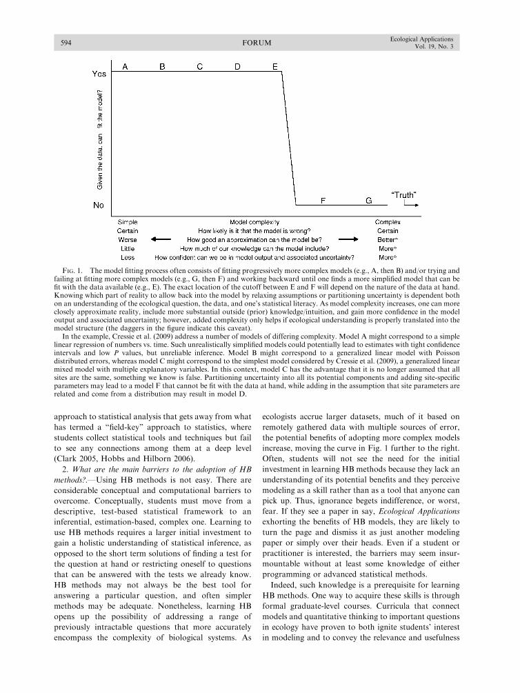
approach to statistical analysis that gets away from what
has termed a ‘‘field-key’’ approach to statistics, where
students collect statistical tools and techniques but fail
to see any connections among them at a deep level
(Clark 2005, Hobbs and Hilborn 2006).
2. What are the main barriers to the adoption of HB
methods?.—Using HB methods is not easy. There are
considerable conceptual and computational barriers to
overcome. Conceptually, students must move from a
descriptive, test-based statistical framework to an
inferential, estimation-based, complex one. Learning to
use HB methods requires a larger initial investment to
gain a holistic understanding of statistical inference, as
opposed to the short term solutions of finding a test for
the question at hand or restricting oneself to questions
that can be answered with the tests we already know.
HB methods may not always be the best tool for
answering a particular question, and often simpler
methods may be adequate. Nonetheless, learning HB
opens up the possibility of addressing a range of
previously intractable questions that more accurately
encompass the complexity of biological systems. As
ecologists accrue larger datasets, much of it based on
remotely gathered data with multiple sources of error,
the potential benefits of adopting more complex models
increase, moving the curve in Fig. 1 further to the right.
Often, students will not see the need for the initial
investment in learning HB methods because they lack an
understanding of its potential benefits and they perceive
modeling as a skill rather than as a tool that anyone can
pick up. Thus, ignorance begets indifference, or worst,
fear. If they see a paper in say, Ecological Applications
exhorting the benefits of HB models, they are likely to
turn the page and dismiss it as just another modeling
paper or simply over their heads. Even if a student or
practitioner is interested, the barriers may seem insur-
mountable without at least some knowledge of either
programming or advanced statistical methods.
Indeed, such knowledge is a prerequisite for learning
HB methods. One way to acquire these skills is through
formal graduate-level courses. Curricula that connect
models and quantitative thinking to important questions
in ecology have proven to both ignite students’ interest
in modeling and to convey the relevance and usefulness
FIG. 1. The model fitting process often consists of fitting progressively more complex models (e.g., A, then B) and/or trying andfailing at fitting more complex models (e.g., G, then F) and working backward until one finds a more simplified model that can befit with the data available (e.g., E). The exact location of the cutoff between E and F will depend on the nature of the data at hand.Knowing which part of reality to allow back into the model by relaxing assumptions or partitioning uncertainty is dependent bothon an understanding of the ecological question, the data, and one’s statistical literacy. As model complexity increases, one can moreclosely approximate reality, include more substantial outside (prior) knowledge/intuition, and gain more confidence in the modeloutput and associated uncertainty; however, added complexity only helps if ecological understanding is properly translated into themodel structure (the daggers in the figure indicate this caveat).
In the example, Cressie et al. (2009) address a number of models of differing complexity. Model A might correspond to a simplelinear regression of numbers vs. time. Such unrealistically simplified models could potentially lead to estimates with tight confidenceintervals and low P values, but unreliable inference. Model B might correspond to a generalized linear model with Poissondistributed errors, whereas model C might correspond to the simplest model considered by Cressie et al. (2009), a generalized linearmixed model with multiple explanatory variables. In this context, model C has the advantage that it is no longer assumed that allsites are the same, something we know is false. Partitioning uncertainty into all its potential components and adding site-specificparameters may lead to a model F that cannot be fit with the data at hand, while adding in the assumption that site parameters arerelated and come from a distribution may result in model D.
FORUM594Ecological Applications
Vol. 19, No. 3

of models. However, many ecology and evolution
programs still rely on statistics departments to train
their students and only a few offer advanced statistical
methods courses within their department. Farming out
ecology students to be trained in statistics departments is
far from ideal because courses are likely to be developed
to address the needs of statistics students rather than
those of other areas of science. If students fail to see the
relevance of the methods to their own discipline,
motivation will decline.
Although there are a number of open, short-term
courses available (Duke University summer course in
ecological forecasting, one-day workshop in Bayesian
methods at the Ecological Society of America annual
meetings), these offerings are limited, unpredictable, and
costly. Moreover, short courses education in HB models
often requires not only some programming skills but a
complete conceptual overhaul of the students’ existing
conceptual statistical framework. Although short
courses may offer an entry into HB models, the tension
between a focus on tools (e.g., WinBUGS) and concepts
is very real when time is limited.
A second way to learn HB is through self-teaching.
Although a few books have appeared in the last couple
of years that make self-teaching possible (Woodworth
2004, Gelman and Hill 2006, Clark 2007, McCarthy
2007), it is still a daunting task to learn these methods on
your own without a support network. Fortunately,
cyber-communities are becoming an increasingly im-
portant form of scientific exchange, and considerable
progress can be made in this way (e.g., contributions and
exchanges around the development and use of R and
WinBUGS Statistical freeware). Auto-didactic ap-
proaches are powerful means to learn but they often
leave behind major lacunas in knowledge because they
tend to focus on the mechanics of carrying out complex
statistical analysis with little attention paid to the
foundations of underlying statistical inference (e.g.,
Taper and Lele 2004).
Another barrier to the adoption of HB is the lack of
consensus in many of the details of implementation. HB
methods are relatively new and there seems to be a lack
of consensus on what are the best non-informative
priors to use, how best to assess convergence, the utility
of deviance information criterion (DIC), etc. This is a
major barrier to biologists who are trying to learn and
implement these methods, since there is often no clear
path to follow. Many ecologists will choose those
methods that they know well despite their shortcomings.
3. What approaches would be most effective in
promoting their use?.—Although there are a small
number of graduate ecology programs that train some
students in modern statistics including HB methods, an
impediment to widespread training teaching in these
methods is the availability of ecology faculty with
statistical background sufficient to offer such courses.
Faculty members need efficient and relevant ways to get
training in modern statistical modeling and the neces-
sary tools and materials to teach them effectively. Given
the time demands placed on faculty, self-education
approaches may be unrealistic. One potential solution
is to offer one-semester sabbatical leaves that interested
faculty could use to attend existing courses at univer-
sities where such courses are offered. Better yet, these
leaves could be structured around the development of
intensive courses that brought together a small group of
expert teachers and student-faculty. The advantages of
this approach are threefold. First, the burden of
teaching could be shared among a small group of
experts. Second, the students would be exposed to a
variety of viewpoints. Third, participating faculty would
gain not only technical and conceptual skills but also a
support network to carry the newly acquired skills back
to their home institutions. This approach would
probably work best with faculty who are already
teaching statistics or use modeling in their research, or
with postdoctoral researchers who have the time and
motivation to learn and use the methods. Costs could be
shared by interested institutions and funding agencies.
In institutions that lack faculty trained in modern
statistical methods, ecology departments could also
work with faculty in the statistics department to develop
advanced courses or at least to discuss statistical issues
and problems as they arise. The advantage of this
approach is that students would be exposed to both the
rigor of statistics and disciplinary applications. The
shortcomings are generating faculty interest and the
considerable investments required to develop a course
with multiple instructors from different disciplines and
departments. Existing or new collaborations between
statisticians and ecologists within the same institution
could be leveraged to this end. Educators in ecology and
other fields that depend on statistics departments for
introductory courses could also initiate a dialog with
their statistical colleagues about restructuring ‘‘service’’
courses to cover basic concepts that are at the heart of
modern statistical methods such as distributional theory.
University administrators could also be approached to
offer faculty incentives for the development of courses
that cross disciplinary boundaries.
Students can also act as catalysts in the adoption of
modern statistics in ecology. Although we caution
against the perils of unabashedly using graduate
students as a means to improve existing programs, both
students and faculty have much to gain from judicious
small-scale efforts. Graduate students are often looking
for teaching opportunities that give them some experi-
ence in curriculum development and allow flexible
didactic approaches. At the same time, faculty members
are also searching for means to increase students’
engagement. One way to address the goals of these
two groups is to allow graduate students to structure
parts of existing course or to have them offer workshops
that provide an introduction to the tools and techniques
that will facilitate self-teaching for other students. For
instance, a short course in R, or structuring labs in
April 2009 595HIERARCHICAL MODELS IN ECOLOGY

existing statistics courses in R software rather than acommercial package, will provide students with some
familiarity with programming and open the door to alarge cyber community with which they can engage. Thisapproach would require some thought on the part of the
faculty and students but could potentially be verypowerful because students readily accept new knowledgeand methods from their peers.
Cyber courses can also be a means to bring statisticalliteracy to ecologists. This approach could make anumber of existing graduate courses in modern statis-
tical methods accessible to ecologists. These coursesinclude among others Ecological Models and Data atthe University of Florida, Ecological Theory and Dataat Duke University, Modeling for Conservation of
Populations at the University of Washington, andSystems Ecology at Colorado State University. Withrelatively minor investments, these courses could be
broadcasted to other graduate program in the UnitedStates and abroad. Although interactions betweenstudents and teaching faculty would be limited, this
approach would provide students with a foundation topursue further education in statistics either through self-teaching or collaboration with statistics faculty at their
home institutions. To encourage use and discussion, thecyber courses could be structured around student–faculty groups at the receiving institutions.Ultimately the widespread adoption of modern
statistical methods will require a mix of approaches.What makes sense for individual institutions will dependon the availability of faculty and on motivations to
develop offerings in this area. Funding agencies can help
by providing incentives to institutions and individual
faculty. To the degree that faculty and students are
interested and willing, statistical literacy can be devel-
oped.
ACKNOWLEDGMENTS
We thank Liza Comita for constructive comments.
LITERATURE CITED
Bolker, B. M. 2008. Ecological models and data in R. PrincetonUniversity Press, Princeton, New Jersey, USA.
Clark, J. S. 2005. Why environmental scientists are becomingBayesians. Ecology Letters 8:2–14.
Clark, J. S. 2007. Models for ecological data: an introduction.Princeton University Press, Princeton, New Jersey, USA.
Clark, J. S., et al. 2001. Ecological forecasts: an emergingimperative. Science 293:657–660.
Cressie, N., C. A. Calder, J. S. Clark, J. M. Ver Hoef, and C. K.Wikle. 2009. Accounting for undertainty in ecologicalanalysis: the strengths and limitations of hierarchicalstatistical analysis. Ecological Applications 19:553–570.
Gelman, A., and J. Hill. 2006. Data analysis using regressionand multilevel/hierarchical models. Cambridge UniversityPress, New York, New York, USA.
Hobbs, N. T., and R. Hilborn. 2006. Alternatives to statisticalhypothesis testing in ecology: a guide to self teaching.Ecology 16:5–19.
McCarthy, M. A. 2007. Bayesian methods for ecology. Cam-bridge University Press, Cambridge, UK.
Pielke, R. A., and R. T. Connant. 2003. Best practices inpredictions for decision-making: lessons from the atmos-pheric and earth sciences. Ecology 84:1351–1358.
Taper, M. L., and S. R. Lele. 2004. The nature of scientificevidence: statistical, philosophical, and empirical consider-ations. University of Chicago Press, Chicago, Illinois, USA.
Woodworth, G. G. 2004. Biostatistics: a Bayesian introduction.Wiley, Hoboken, New Jersey, USA.
FORUM596Ecological Applications
Vol. 19, No. 3
Recommended