Course:
Optimization III
Convex Analysis
Nonlinear Programming Theory
Nonlinear Programming Algorithms
ISyE 6663 Spring 2008
Lecturer: Prof. Arkadi Nemirovski
Lecture Notes, Transparencies, Assignments:
https://t-square.gatech.edu/portal/site/21746.200802
Grading Policy:
Assignments 5%Midterm exam I 20%Midterm exam II 25%Final exam 50%
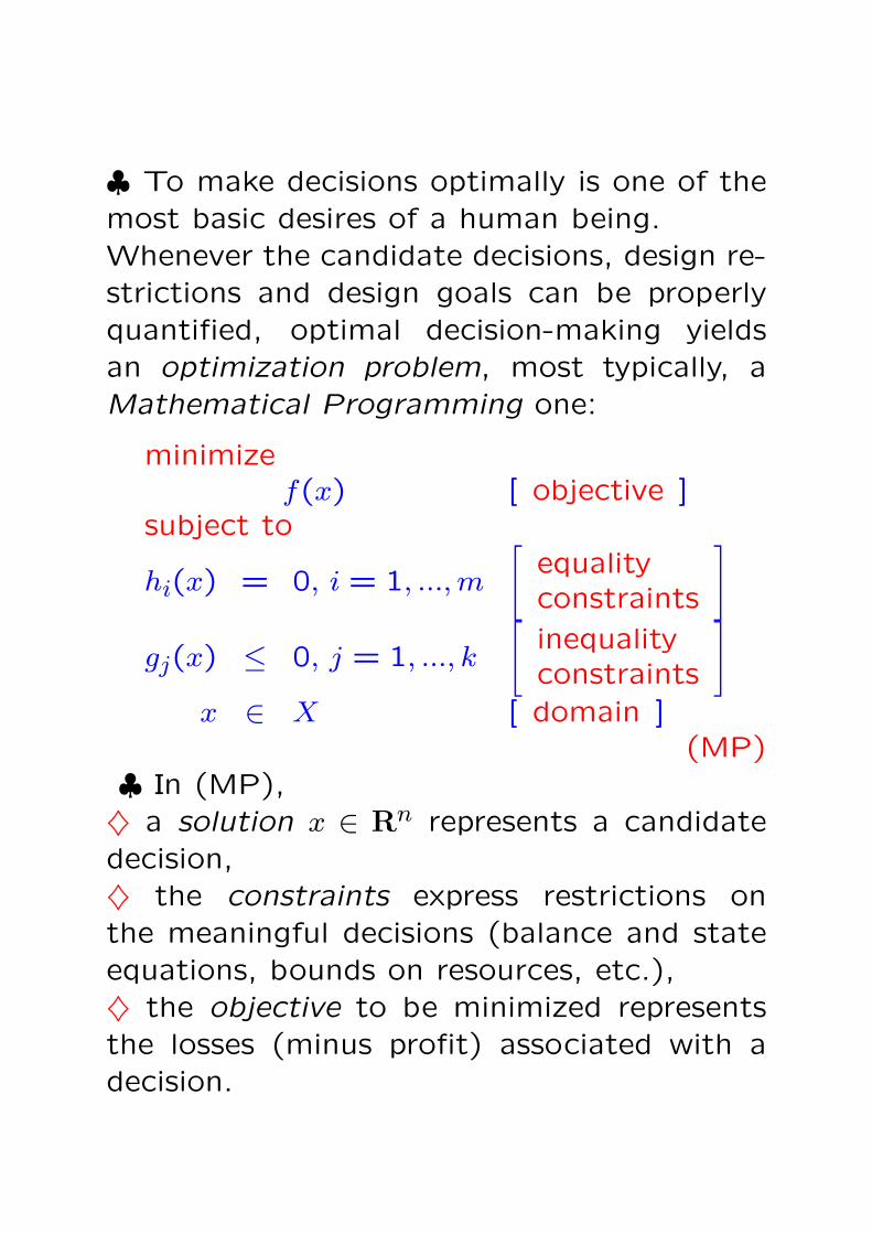
♣ To make decisions optimally is one of themost basic desires of a human being.Whenever the candidate decisions, design re-strictions and design goals can be properlyquantified, optimal decision-making yieldsan optimization problem, most typically, aMathematical Programming one:
minimizef(x) [ objective ]
subject to
hi(x) = 0, i = 1, ..., m
[equalityconstraints
]
gj(x) ≤ 0, j = 1, ..., k
[inequalityconstraints
]
x ∈ X [ domain ](MP)
♣ In (MP),♦ a solution x ∈ Rn represents a candidatedecision,♦ the constraints express restrictions onthe meaningful decisions (balance and stateequations, bounds on resources, etc.),♦ the objective to be minimized representsthe losses (minus profit) associated with adecision.

minimizef(x) [ objective ]
subject to
hi(x) = 0, i = 1, ..., m
[equalityconstraints
]
gj(x) ≤ 0, j = 1, ..., k
[inequalityconstraints
]
x ∈ X [ domain ](MP)
♣ To solve problem (MP) means to find its
optimal solution x∗, that is, a feasible (i.e.,
satisfying the constraints) solution with the
value of the objective ≤ its value at any other
feasible solution:
x∗ :
hi(x∗) = 0∀i & gj(x∗) ≤ 0 ∀j & x∗ ∈ X
hi(x) = 0∀i & gj(x) ≤ 0∀j & x ∈ X
⇒ f(x∗) ≤ f(x)

minx
f(x)
s.t.hi(x) = 0, i = 1, ..., mgj(x) ≤ 0, j = 1, ..., k
x ∈ X
(MP)
♣ In Combinatorial (or Discrete) Optimiza-
tion, the domain X is a discrete set, like the
set of all integral or 0/1 vectors.
In contrast to this, in Continuous Optimiza-
tion we will focus on, X is a “continuum”
set like the entire Rn,a box x : a ≤ x ≤ b,or simplex x ≥ 0 :
∑j
xj = 1, etc., and the
objective and the constraints are (at least)
continuous on X.
♣ In Linear Programming, X = Rn and the
objective and the constraints are linear func-
tions of x.
In contrast to this, in Nonlinear Continuous
Optimization, the objective and/or some of
the constraints are nonlinear.

minx
f(x)
s.t.hi(x) = 0, i = 1, ..., mgj(x) ≤ 0, j = 1, ..., k
x ∈ X
(MP)
♣ The goals of our course is to present
• basic theory of Continuous Optimization,with emphasis on existence and unique-ness of optimal solutions and their char-acterization (i.e., necessary and/or suffi-cient optimality conditions);
• traditional algorithms for building (ap-proximate) optimal solutions to Contin-uous Optimization problems.
♣ Mathematical foundation of OptimizationTheory is given by Convex Analysis – a spe-cific combination of Real Analysis and Geom-etry unified by and focusing on investigatingconvexity-related notions.
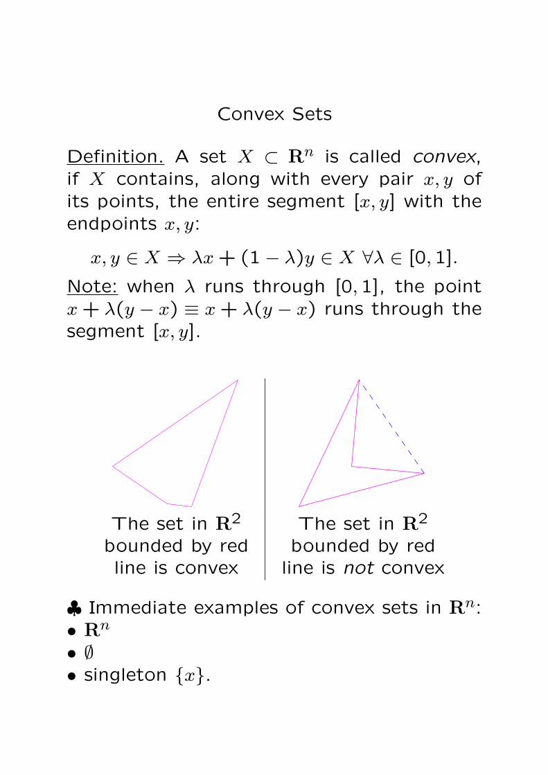
Convex Sets
Definition. A set X ⊂ Rn is called convex,if X contains, along with every pair x, y ofits points, the entire segment [x, y] with theendpoints x, y:
x, y ∈ X ⇒ λx + (1− λ)y ∈ X ∀λ ∈ [0,1].
Note: when λ runs through [0,1], the pointx + λ(y − x) ≡ x + λ(y − x) runs through thesegment [x, y].
The set in R2
bounded by redline is convex
The set in R2
bounded by redline is not convex
♣ Immediate examples of convex sets in Rn:• Rn
• ∅• singleton x.
Examples of convex sets, I: Affine sets
Definition: Affine set M in Rn is a set which
can be obtained as a shift of a linear subspace
L ⊂ Rn by a vector a ∈ Rn:
M = a + L = x = a + y : y ∈ L (1)
Note: I. The linear subspace L is uniquely
defined by affine subspace M and is the set
of differences of vectors from M :
(1) ⇒ L = M −M = y = x′− x′′ : x′, x′′ ∈ M
II. The shift vector a is not uniquely defined
by affine subspace M ; in (1), one can take as
a every vector from M (and only vector from
M):
(1) ⇒ M = a′ + L ∀a′ ∈ M.

III. Generic example of affine subspace: theset of solutions of a solvable system of linearequations:
M is affine subspace in Rn
m∅ 6= M ≡ x ∈ Rn : Ax = b ≡ a︸︷︷︸
Aa=b
+ x : Ax = 0︸ ︷︷ ︸KerA
♣ By III, affine subspace is convex, due toProposition. The solution set of an arbitrary(finite or infinite) system of linear inequalitiesis convex:
X = x ∈ Rn : aTαx ≤ bα, α ∈ A ⇒ X is convex
In particular, every polyhedral set x : Ax ≤ bis convex.Proof:
x, y ∈ X, λ ∈ [0,1]
⇔ aTαx ≤ bα, aT
αy ≤ bα∀α ∈ A, λ ∈ [0,1]
⇒ λaTαx + (1− λ)aT
αy︸ ︷︷ ︸aT
α[λx+(1−λ)y]
≤ λbα + (1− λ)bα︸ ︷︷ ︸bα
∀α ∈ A
⇒ [λx + (1− λ)y] ∈ X ∀λ ∈ [0,1].
Remark: Proposition remains valid when part
of the nonstrict inequalities aTαx ≤ bα are re-
placed with their strict versions aTαx < bα.
Remark: The solution set
X = x : aTαx ≤ bα, α ∈ A
of a system of nonstrict inequalities is not
only convex, it is closed (i.e., contains limits
of all converging sequences xi ∈ X∞i=1 of
points from X).
We shall see in the mean time that
Vice versa, every closed and convex set
X ⊂ Rn is the solution set of an appropriate
countable system of nonstrict linear inequal-
ities:
X is closed and convex⇓
X = x : aTi x ≤ bi, i = 1,2, ...

Examples of convex sets, II: Unit balls ofnorms
Definition: A real-valued function ‖x‖ on Rn
is called a norm, if it possesses the followingthree properties:♦ [positivity] ‖x‖ ≥ 0 for all x and ‖x‖ = 0 iffx = 0;♦ [homogeneity] ‖λx‖ = |λ|‖x‖ for all vectorsx and reals λ;♦ [triangle inequality] ‖x+ y‖ ≤ ‖x‖+ ‖y‖ forall vectors x, y.Proposition: Let ‖ · ‖ be a norm on Rn. Theunit ball of this norm – the set x : ‖x‖ ≤ 1,same as any other ‖ · ‖-ball x : ‖x− a‖ ≤ r,is convex.Proof:
‖x− a‖ ≤ r, ‖y − a‖ ≤ r, λ ∈ [0,1]
⇒ λ‖x− a‖+ (1− λ)‖y − a‖︸ ︷︷ ︸= ‖λ(x− a)‖+ ‖(1− λ)(y − a)‖≥ ‖λ(x− a) + (1− λ)(y − a)‖= ‖[λx + (1− λ)y]− a‖
≤ λr + (1− λ)r︸ ︷︷ ︸r
⇒ ‖[λx + (1− λ)y]− a‖ ≤ r ∀λ ∈ [0,1].

Standard examples of norms on Rn: `p-norms
‖x‖p =
(n∑
i=1|xi|p
)1/p
, 1 ≤ p < ∞max
i|xi|, p = ∞
Note: • ‖x‖2 =√∑
ix2
i is the standard Eu-
clidean norm;
• ‖x‖1 =∑i|xi|;
• ‖x‖∞ = maxi|xi| (uniform norm).
Note: except for the cases p = 1 and p = ∞,
triangle inequality for ‖·‖p requires a nontriv-
ial proof!
Proposition [characterization of ‖ · ‖-balls] A
set U in Rn is the unit ball of a norm iff U is
(a) convex and symmetric w.r.t. 0: V = −V ,
(b) bounded and closed, and
(c) contains a neighbourhood of the origin.
Examples of convex sets, III: Ellipsoid
Definition: An ellipsoid in Rn is a set X givenby♦ positive definite and symmetric n×n matrixQ (that is, Q = QT and uTQu > 0 wheneveru 6= 0),♦ center a ∈ Rn,♦ radius r > 0via the relation
X = x : (x− a)TQ(x− a) ≤ r2.
Proposition: An ellipsoid is convex.
Proof: Since Q is symmetric positive def-inite, by Linear Algebra Q = (Q1/2)2 foruniquely defined symmetric positive definitematrix Q1/2. Setting ‖x‖Q = ‖Q1/2x‖2, weclearly get a norm on Rn (since ‖ · ‖2 is anorm and Q1/2 is nonsingular). We have
(x− a)TQ(x− a) = [(x− a)TQ1/2][Q1/2(x− a)]= ‖Q1/2(x− a)‖22 = ‖x− a‖2Q,
so that X is a ‖ · ‖Q-ball and is therefore aconvex set.

Examples of convex sets, IV:ε-neighbourhood of convex set
Proposition: Let M be a nonempty convexset in Rn, ‖ · ‖ be a norm, and ε ≥ 0. Thenthe set
X = x : dist‖·‖(x, M) ≡ infy∈M
‖x− y‖ ≤ ε
is convex.
Proof: x ∈ X if and only if for every ε′ > ε
there exists y ∈ M such that ‖x− y‖ ≤ ε′. Wenow have
x, y ∈ X, λ ∈ [0,1]
⇒ ∀ε′ > ε∃u, v ∈ M : ‖x− u‖ ≤ ε′, ‖y − v‖ ≤ ε′
⇒ ∀ε′ > ε∃u, v ∈ M :λ‖x− u‖+ (1− λ)‖y − v‖︸ ︷︷ ︸≥‖[λx+(1−λ)y]−[λu+(1−λ)v]‖
≤ ε′ ∀λ ∈ [0,1]
⇒ ∀ε′ > ε ∀λ ∈ [0,1]∃w = λu + (1− λ)v ∈ M :‖[λx + (1− λ)y]− w‖ ≤ ε′
⇒ λx + (1− λ)y ∈ X ∀λ ∈ [0,1]
Convex Combinations and Convex Hulls
Definition: A convex combination of m vec-
tors x1, ..., xm ∈ Rn is their linear combination∑
i
λixi
with nonnegative coefficients and unit sum
of the coefficients:
λi ≥ 0 ∀i,∑
i
λi = 1.

Proposition: A set X ⊂ Rn is convex iff it is
closed w.r.t. taking convex combinations of
its points:
X is convexm
xi ∈ X, λi ≥ 0,∑i
λi = 1 ⇒ ∑i
λixi ∈ X.
Proof, ⇒: Assume that X is convex, and
let us prove by induction in k that every k-
term convex combination of vectors from X
belongs to X. Base k = 1 is evident. Step
k ⇒ k + 1: let x1, ..., xk+1 ∈ X and λi ≥ 0,k∑
i=1λi = 1; we should prove that
k+1∑i=1
λixi ∈ X.
Assume w.l.o.g. that 0 ≤ λk+1 < 1. Then
k+1∑i=1
λixi = (1− λk+1)
( k∑
i=1
λi
1− λk+1xi
︸ ︷︷ ︸∈X
)
+λk+1xk+1 ∈ X.
Proof, ⇐: evident, since the definition of
convexity of X is nothing but the require-
ment for every 2-term convex combination
of points from X to belong to X.

Proposition: The intersection X =⋂
α∈AXα of
an arbitrary family Xαα∈A of convex sub-
sets of Rn is convex.
Proof: evident.
Corollary: Let X ⊂ Rn be an arbitrary set.
Then among convex sets containing X (which
do exist, e.g. Rn) there exists the smallest
one, namely, the intersection of all convex
sets containing X.
Definition: The smallest convex set contain-
ing X is called the convex hull Conv(X) of X.

Proposition [convex hull via convex combina-
tions] For every subset X of Rn, its convex
hull Conv(X) is exactly the set X of all con-
vex combinations of points from X.
Proof. 1) Every convex set which con-
tains X contains every convex combination of
points from X as well. Therefore Conv(X) ⊃X.
2) It remains to prove that Conv(X) ⊂ X. To
this end, by definition of Conv(X), it suffices
to verify that the set X contains X (evident)
and is convex. To see that X is convex, let
x =∑i
νixi, y =∑i
µixi be two points from X
represented as convex combinations of points
from X, and let λ ∈ [0,1]. We have
λx + (1− λ)y =∑
i
[λνi + (1− λ)µi]xi,
i.e., the left hand side vector is a convex com-
bination of vectors from X.
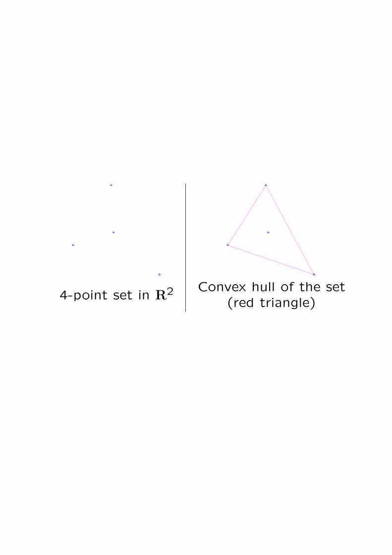
4-point set in R2 Convex hull of the set(red triangle)

Examples of convex sets, V: simplex
Definition: A collection of m+1 points xi, i =
0, ..., m, in Rn is called affine independent, if
no nontrivial combination of the points with
zero sum of the coefficients is zero:
x0, ..., xm are affine independentm
m∑i=0
λixi = 0 &∑i
λi = 0 ⇒ λi = 0,0 ≤ i ≤ m
Motivation: Let X ⊂ Rn be nonempty.
I. For every nonempty set X ∈ Rn, the in-
tersection of all affine subspaces containing
X is an affine subspace. This clearly is the
smallest affine subspace containing X; it is
called the affine hull Aff(X) of X.
II. It is easily seen that Aff(X) is nothing but
the set of all affine combinations of points
from X, that is, linear combinations with unit
sum of coefficients:
Aff(X) = x =∑
i
λixi : xi ∈ X,∑
i
λi = 1.

III. m + 1 points x0, ..., xm are affinely inde-
pendent iff every point x ∈ Aff(x0, ..., xm) of
their affine hull can be uniquely represented
as an affine combination of x0, ..., xm:∑
i
λixi =∑
i
µixi &∑
i
λi =∑
i
µi = 1 ⇒ λi ≡ µi
In this case, the coefficients λi in the repre-
sentation
x =m∑
i=0
λixi [∑i
λi = 1]
of a point x ∈ M = Aff(x0, ..., xm) as an
affine combination of x0, ..., xm are called the
barycentric coordinates of x ∈ M taken w.r.t.
affine basis x0, ..., xm of M .

Definition: m-dimensional simplex ∆ with
vertices x0, ..., xm is the convex hull of m + 1
affine independent points x0, ..., xm:
∆ = ∆(x0, ..., xm) = Conv(x0, ..., xm).Examples: A. 2-dimensional simplex is given
by 3 points not belonging to a line and is the
triangle with vertices at these points.
B. Let e1, ..., en be the standard basic or-
ths in Rn. These n points are affinely in-
dependent, and the corresponding (n − 1)-
dimensional simplex is the standard simplex
∆n = x ∈ Rn : x ≥ 0,∑i
xi = 1.C. Adding to e1, ..., en the vector e0 = 0, we
get n+1 affine independent points. The cor-
responding n-dimensional simplex is
∆+n = x ∈ Rn : x ≥ 0,
∑i
xi ≤ 1.Simplex with vertices x0, ..., xm is convex (as
a convex hull of a set), and every point from
the simplex is a convex combination of the
vertices with the coefficients uniquely defined
by the point.
Examples of convex sets, VI: cone
Definition: A nonempty subset K of Rn is
called conic, if it contains, along with every
point x, the entire ray emanating from the
origin and passing through x:
K is conicm
K 6= ∅ & ∀(x ∈ K, t ≥ 0) : tx ∈ K.
A convex conic set is called a cone.
Examples: A. Nonnegative orthant
Rn+ = x ∈ Rn : x ≥ 0
B. Lorentz cone
Ln = x ∈ Rn : xn ≥√
x21 + ... + x2
n−1C. Semidefinite cone Sn
+. This cone “lives”
in the space Sn of n× n symmetric matrices
and is comprised of all positive semidefinite
symmetric n× n matrices
D. The solution set x : aTαx ≤ 0∀α ∈ A
of an arbitrary (finite or infinite) homoge-neous system of nonstrict linear inequalitiesis a closed cone. In particular, so is a poly-hedral cone x : Ax ≤ 0.Note: Every closed cone in Rn is the solutionset of a countable system of nonstrict linearinequalities.
Proposition: A nonempty subset K of Rn isa cone iff♦ K is conic: x ∈ K, t ≥ 0 ⇒ tx ∈ K, and♦ K is closed w.r.t. addition:
x, y ∈ K ⇒ x + y ∈ K.Proof, ⇒: Let K be convex and x, y ∈ K,Then 1
2(x + y) ∈ K by convexity, and sinceK is conic, we also have x + y ∈ K. Thus, aconvex conic set is closed w.r.t. addition.Proof, ⇐: Let K be conic and closed w.r.t.addition. In this case, a convex combinationλx + (1 − λ)y of vectors x, y from K is thesum of the vectors λx and (1− λ)y and thusbelongs to K, since K is closed w.r.t. addi-tion. Thus, a conic set which is closed w.r.t.addition is convex.
♣ Cones form an extremely important class
of convex sets with properties “parallel” to
those of general convex sets. For example,
♦ Intersection of an arbitrary family of cones
again is a cone. As a result, for every
nonempty set X, among the cones containing
X there exists the smallest cone Cone (X),
called the conic hull of X.
♦ A nonempty set is a cone iff it is closed
w.r.t. taking conic combinations of its ele-
ments (i.e., linear combinations with nonneg-
ative coefficients).
♦ The conic hull of a nonempty set X is
exactly the set of all conic combinations of
elements of X.

“Calculus” of Convex Sets
Proposition. The following operations pre-
serve convexity of sets:
1. Intersection: If Xα ⊂ Rn, α ∈ A, are
convex sets, so is⋂
α∈AXα
2. Direct product: If X` ⊂ Rn` are convex
sets, ` = 1, ..., L, so is the set
X = X1 × ...×XL
≡ x = (x1, ..., xL) : x` ∈ X`,1 ≤ ` ≤ L⊂ Rn1+...+nL
3. Taking weighted sums: Let X1, ..., XL
be nonempty convex subsets in Rn and
λ1, ..., λL be reals. Then the set
λ1X1 + ... + λLXL≡ x = λ1x1 + ... + λLx` : x` ∈ X`,1 ≤ ` ≤ Lis convex.

4. Affine image: Let X ⊂ Rn be convex
and x 7→ A(x) = Ax+ b be an affine mapping
from Rn to Rk. Then the image of X under
the mapping – the set
A(X) = y = Ax + b : x ∈ Xis convex.
5. Inverse affine image: Let X ⊂ Rn be
convex and y 7→ A(y) = Ay + b be an affine
mapping from Rk to Rn. Then the inverse
image of X under the mapping – the set
A−1(X) = y : Ay + b ∈ Xis convex.
Application example: A point x ∈ Rn is
(a) “good”, if it satisfies a given system of
linear constraints Ax ≤ b,
(b) “excellent”, if it dominates a good point:
∃y: y is good and x ≥ y,
(c) “semi-excellent”, if it can be approxi-
mated, within accuracy 0.1 in the coordinate-
wise fashion, by excellent points:
∀(i, ε′ > 0.1)∃y : |yi − xi| ≤ ε′ & y is excellent
Question: Whether the set of semi-excellent
points is convex?
Answer: Yes. Indeed,
• The set Xg of good points is convex (as a
polyhedral set)
• ⇒ The set Xexc of excellent points is con-
vex (as the sum of convex set Xg and the
nonnegative orthant Rn+, which is convex)
• ⇒ For every i, the set Xiexc of i-th coor-
dinates of excellent points is convex (as the
projection of Xexc onto i-th axis; projection
is an affine mapping)
• ⇒ For every i, the set Y i on the axis which
is the 0.1-neighbourhood of Xiexc, is convex
(as 0.1-neighbourhood of a convex set)
• ⇒ The set of semi-excellent points, which
is the direct product of the sets Y 1,..., Y n,
is convex (as direct product of convex sets).
Nice Topological Properties of Convex Sets
♣ Recall that the set X ⊂ Rn is called♦ closed, if X contains limits of all converg-ing sequences of its points:
xi ∈ X & xi → x, i →∞⇒ x ∈ X
♦ open, if it contains, along with every of itspoints x, a ball of a positive radius centeredat x:
x ∈ X ⇒ ∃r > 0 : y : ‖y − x‖2 ≤ r ⊂ X.
E.g., the solution set of an arbitrary systemof nonstrict linear inequalities x : aT
αx ≤ bαis closed; the solution set of finite system ofstrict linear inequalities x : Ax < b is open.
Facts: A. X is closed iff Rn\X is openB. The intersection of an arbitrary family ofclosed sets and the union of a finite family ofclosed sets are closedB′. The union of an arbitrary family of opensets and the intersection of a finite family ofopen sets are open
♦ From B it follows that the intersection of
all closed sets containing a given set X is
closed; this intersection, called the closure
clX of X, is the smallest closed set contain-
ing X. clX is exactly the set of limits of all
converging sequences of points of X:
clX = x : ∃xi ∈ X : x = limi→∞xi.
♦ From B′ it follows that the union of all
open sets contained in a given set X is open;
this union, called the interior intX of X, is
the largest open set contained X. intX is
exactly the set of all interior points of X –
points x belonging to X along with balls of
positive radii centered at the points:
intX = x : ∃r > 0 : y : ‖y − x‖2 ≤ r ⊂ X.♦ Let X ⊂ Rn. Then intX ⊂ X ⊂ clX.
The “difference” ∂X = clX\intX is called the
boundary of X; boundary always is closed (as
the intersection of the closed sets clX and
the complement of intX).

intX ⊂ X ⊂ clX (∗)♣ In general, the discrepancy between intX
and clX can be pretty large.
E.g., let X ⊂ R1 be the set of irrational num-
bers in [0,1]. Then intX = ∅, clX = [0,1],
so that intX and clX differ dramatically.
♣ Fortunately, a convex set is perfectly well
approximated by its closure (and by interior,
if the latter is nonempty).
Proposition: Let X ⊂ Rn be a nonempty con-
vex set. Then
(i) Both intX and clX are convex
(ii) If intX is nonempty, then intX is dense
in clX. Moreover,
x ∈ intX, y ∈ clX ⇒λx + (1− λ)y ∈ intX ∀λ ∈ (0,1]
(!)
• Claim (i): Let X be convex. Then both
intX and clX are convex
Proof. (i) is nearly evident. Indeed, to prove
that intX is convex, note that for every two
points x, y ∈ intX there exists a common
r > 0 such that the balls Bx, By of radius
r centered at x and y belong to X. Since X
is convex, for every λ ∈ [0,1] X contains the
set λBx + (1 − λ)By, which clearly is noth-
ing but the ball of the radius r centered at
λx+(1−λ)y. Thus, λx+(1−λ)y ∈ intX for
all λ ∈ [0,1].
Similarly, to prove that clX is convex, assume
that x, y ∈ clX, so that x = limi→∞ xi and
y = limi→∞ yi for appropriately chosen xi, yi ∈ X.
Then for λ ∈ [0,1] we have
λx + (1− λ)y = limi→∞ [λxi + (1− λ)yi]︸ ︷︷ ︸
∈X
,
so that λx + (1− λ)y ∈ clX for all λ ∈ [0,1].
• Claim (ii): Let X be convex and intX be
nonempty. Then intX is dense in clX; more-
over,
x ∈ intX, y ∈ clX ⇒λx + (1− λ)y ∈ intX ∀λ ∈ (0,1]
(!)
Proof. It suffices to prove (!). Indeed, let
x ∈ intX (the latter set is nonempty). Ev-
ery point x ∈ clX is the limit of the sequence
xi = 1i x +
(1− 1
i
)x. Given (!), all points xi
belong to intX, thus intX is dense in clX.
• Claim (ii): Let X be convex and intX be
nonempty. Then
x ∈ intX, y ∈ clX ⇒λx + (1− λ)y ∈ intX ∀λ ∈ (0,1]
(!)
Proof of (!): Let x ∈ intX, y ∈ clX, λ ∈(0,1]. Let us prove that λx+(1−λ)y ∈ intX.
Since x ∈ intX, there exists r > 0 such that
the ball B of radius r centered at x belongs
to X. Since y ∈ clX, there exists a sequence
yi ∈ X such that y = limi→∞ yi. Now let
Bi = λB + (1− λ)yi= z = [λx + (1− λ)yi]︸ ︷︷ ︸
zi
+λd : ‖d‖2 ≤ r
≡ z = zi + ∆ : ‖δ‖ ≤ r′ = λd.Since B ⊂ X, yi ∈ X and X is convex, the sets
Bi (which are balls of radius r′ > 0 centered
at zi) contain in X. Since zi → z = λx +
(1 − λ)y as i → ∞, all these balls, starting
with certain number, contain the ball B′ of
radius r′/2 centered at z. Thus, B′ ⊂ X, i.e.,
z ∈ intX.
♣ Let X be a convex set. It may happen thatintX = ∅ (e.g., X is a segment in 3D); in thiscase, interior definitely does not approximateX and clX. What to do?The natural way to overcome this difficulty isto pass to relative interior, which is nothingbut the interior of X taken w.r.t. the affinehull Aff(X) of X rather than to Rn. Thisaffine hull, geometrically, is just certain Rm
with m ≤ n; replacing, if necessary, Rn withthis Rm, we arrive at the situation where intXis nonempty.Implementation of the outlined idea goesthrough the followingDefinition: [relative interior and relative bound-ary] Let X be a nonempty convex set and M
be the affine hull of X. The relative interiorrint X is the set of all point x ∈ X such thata ball in M of a positive radius, centered atx, is contained in X:
rint X = x : ∃r > 0 :y ∈ Aff(X), ‖y − x‖2 ≤ r ⊂ X.
The relative boundary of X is, by definition,clX\rint X.

Note: An affine subspace M is given by a
list of linear equations and thus is closed; as
such, it contains the closure of every sub-
set Y ⊂ M ; this closure is nothing but the
closure of Y which we would get when re-
placing the original “universe” Rn with the
affine subspace M (which, geometrically, is
nothing but Rm with certain m ≤ n).
The essence of the matter is in the following
fact:
Proposition: Let X ⊂ Rn be a nonempty con-
vex set. Then rint X 6= ∅.
♣ Thus, replacing, if necessary, the original
“universe” Rn with a smaller geometrically
similar universe, we can reduce investigating
an arbitrary nonempty convex set X to the
case where this set has a nonempty interior
(which is nothing but the relative interior of
X). In particular, our results for the “full-
dimensional” case imply that
For a nonempty convex set X, both rint X
and clX are convex sets such that
∅ 6= rint X ⊂ X ⊂ clX ⊂ Aff(X)
and rint X is dense in clX. Moreover, when-
ever x ∈ rint X, y ∈ clX and λ ∈ (0,1], one
has
λx + (1− λ)y ∈ rint X.
∅ 6= X is convex ?? ⇒ ?? rint X 6= ∅
Proof. 10. Shifting X, we may assume
w.l.o.g. that 0 ∈ X, so that Aff(X) is merely
a linear subspace L in Rn.
20. It may happen that L = 0. Here
X = 0 = L, whence the interior of X taken
w.r.t. L is X and thus is nonempty.

30. Now let L 6= 0. Since 0 ∈ X, L =
Aff(X) (which always is the set of all affine
combinations of vectors from X) is the same
as the set of all linear combinations of vectors
from X, i.e., is the linear span of X. Since
dimL > 0, we can choose in L a linear basis
e1, ..., em with e1, ..., em ∈ X. Setting e0 = 0 ∈X, we get m + 1 affine independent vectors
e0, ..., em in X. Since X is convex, the simplex
∆ with vertices e0 = 0, e1, ..., em is contained
in X. Thus,
X ⊃ ∆ = x =m∑
i=0λiei : λ ≥ 0,
m∑i=0
λi = 1
⊃ x =m∑
i=1λiei : λ1, ..., λm > 0,
m∑i=1
λi < 1.
We see that X contains all vectors from L
for which the coordinates w.r.t. the basis
e1, ..., em are positive and with sum < 1.
This set is open in L. Thus, the interior of
X w.r.t. L is nonempty.

♣ Let X be convex and x ∈ rint X. As we
know,
λ ∈ [0,1], y ∈ clX ⇒ yλ = λx + (1− λ)y ∈ X.
It follows that in order to pass from X to its
closure clX, it suffices to pass to “radial clo-
sure”:
For every direction 0 6= d ∈ Aff(X) − x, let
Td = t ≥ 0 : x + td ∈ X.Note: Td is a convex subset of R+ which con-
tains all small enough positive t’s.
♦ If Td is unbounded or is a bounded seg-
ment: Td = t : 0 ≤ t ≤ t(d) < ∞, the inter-
section of clX with the ray x + td : t ≥ 0is exactly the same as the intersection of X
with the same ray.
♦ If Td is a bounded half-segment: Td = t :
0 ≤ t < t(d) < ∞, the intersection of clX
with the ray x+ td : t ≥ 0 is larger than the
intersection of X with the same ray by ex-
actly one point, namely, x+ t(d)d. Adding to
X these “missing points” for all d, we arrive
at clX.

Main Theorems on Convex Sets, I:
Caratheodory Theorem
Definition: Let M be affine subspace in Rn,
so that M = a + L for a linear subspace L.
The linear dimension of L is called the affine
dimension dimM of M .
Examples: The affine dimension of a single-
ton is 0. The affine dimension of Rn is n.
The affine dimension of an affine subspace
M = x : Ax = b is n−Rank(A).
For a nonempty set X ⊂ Rn, the affine di-
mension dimX of X is exactly the affine di-
mension of the affine hull Aff(X) of X.
Theorem [Caratheodory] Let ∅ 6= X ⊂ Rn.
Then every point x ∈ Conv(X) is a convex
combination of at most dim(X) + 1 points
of X.

Theorem [Caratheodory] Let ∅ 6= X ⊂ Rn.
Then every point x ∈ Conv(X) is a convex
combination of at most dim(X) + 1 points
of X.
Proof. 10. We should prove that if x is a
convex combination of finitely many points
x1, ..., xk of X, then x is a convex combina-
tion of at most m +1 of these points, where
m = dim(X). Replacing, if necessary, Rn
with Aff(X), it suffices to consider the case
of m = n.
20. Consider a representation of x as a con-
vex combination of x1, ..., xk with minimum
possible number of nonzero coefficients; it
suffices to prove that this number is ≤ n+1.
Let, on the contrary, the “minimum repre-
sentation” of x
x =p∑
i=1
λixi [λi ≥ 0,∑i
λi = 1]
has p > nm + 1 terms.

30. Consider the homogeneous system of
linear equations in p variables δi
(a)p∑
i=1δixi = 0 [n linear equations]
(b)∑i
δi = 0 [single linear equation]
Since p > n + 1, this system has a nontrivial
solution δ. Observe that for every t ≥ 0 one
has
x =p∑
i=1
[λi + tδi]︸ ︷︷ ︸λi(t)
xi &∑
i
λi(t) = 1.
δ : δ 6= 0 &∑i
δi = 0
∀t ≥ 0 : x =p∑
i=1[λi + tδi]︸ ︷︷ ︸
λi(t)
xi &∑i
λi(t) = 1.
♦ When t = 0, all coefficients λi(t) are non-negative♦ When t → ∞, some of the coefficientsλi(t) go to −∞ (indeed, otherwise we wouldhave δi ≥ 0 for all i, which is impossible since∑i
δi = 0 and not all δi are zeros).
♦ It follows that the quantity
t∗ = max t : t ≥ 0 & λi(t) ≥ 0∀iis well defined; when t = t∗, all coefficientsin the representation
x =p∑
i=1
λi(t∗)xi
are nonnegative, sum of them equals to 1,and at least one of the coefficients λi(t∗)vanishes. This contradicts the assumptionof minimality of the original representationof x as a convex combination of xi.
Theorem [Caratheodory, Conic Version.] Let
∅ 6= X ⊂ Rn. Then every vector x ∈ Cone (X)
is a conic combination of at most n vectors
from X.
Remark: The bounds given by Caratheodory
Theorems (usual and conic version) are sharp:
♦ for a simplex ∆ with m+1 vertices v0, ..., vm
one has dim∆ = m, and it takes all the ver-
tices to represent the barycenter 1m+1
m∑i=0
vi
as a convex combination of the vertices;
♦ The conic hull of n standard basic orths
in Rn is exactly the nonnegative orthant Rn+,
and it takes all these vectors to get, as their
conic combination, the n-dimensional vector
of ones.

Problem: Supermarkets sell 99 different herbal
teas; every one of them is certain blend of
26 herbs A,...,Z. In spite of such a variety of
marketed blends, John is not satisfied with
any one of them; the only herbal tea he likes
is their mixture, in the proportion
1 : 2 : 3 : ... : 98 : 99
Once it occurred to John that in order to pre-
pare his favorite tea, there is no necessity to
buy all 99 marketed blends; a smaller number
of them will do. With some arithmetics, John
found a combination of 66 marketed blends
which still allows to prepare his tea. Do you
believe John’s result can be improved?
Theorem [Radon] Let x1, ..., xm be m ≥ n+2vectors in Rn. One can split these vec-tors into two nonempty and non-overlappinggroups A, B such that
Conv(A) ∩Conv(B) 6= ∅.Proof. Consider the homogeneous system
of linear equations in m variables δi:
m∑i=1
δixi = 0 [n linear equations]
m∑i=1
δi = 0 [single linear equation]
Since m ≥ n + 2, the system has a nontrivialsolution δ. Setting I = i : δi > 0, J =i : δi ≤ 0, we split the index set 1, ..., minto two nonempty (due to δ 6= 0,
∑i
uδi = 0)
groups such that∑i∈I
δixi =∑
j∈J[−δj]xj
γ =∑i∈I
δi =∑
j∈J−δj > 0
whence∑
i∈I
δi
γxi
︸ ︷︷ ︸∈Conv(xi:i∈A)
=∑
j∈J
−δj
γxj
︸ ︷︷ ︸∈Conv(xj:j∈B)
.

Theorem [Helley] Let A1, ..., AM be convex
sets in Rn. Assume that every n+1 sets from
the family have a point in common. Then all
sets also have point in common.
Proof: induction in M . Base M ≤ n + 1 is
trivially true.
Step: Assume that for certain M ≥ n + 1
our statement hods true for every M-member
family of convex sets, and let us prove that it
holds true for M+1-member family of convex
sets A1, ..., AM+1.
♦ By inductive hypotheses, every one of the
M + 1 sets
B` = A1 ∩A2 ∩ ... ∩A`−1 ∩A`+1 ∩ ... ∩AM+1
is nonempty. Let us choose x` ∈ B`,
` = 1, ..., M + 1. ♦ By Radon’s Theorem,
the collection x1, ..., xM+1 can be split in
two sub-collections with intersecting convex
hulls. W.l.o.g., let the split be x1, ..., xJ−1∪xJ , ..., xM+1, and let
z ∈ Conv(x1, ..., xJ−1)⋂
Conv(xJ , ..., xM+1).
Situation: xj belongs to all sets A` except,
perhaps, for Aj and
z ∈ Conv(x1, ..., xJ−1)⋂
Conv(xJ , ..., xM+1).
Claim: z ∈ A` for all ` ≤ M + 1 (Q.E.D.)
Indeed, for ` ≤ J−1, the points xJ , xJ+1, ..., xM+1
belong to the convex set A`, whence
z ∈ Conv(xJ , ..., xM+1) ⊂ A`.
For ` ≥ J, the points x1, ..., xJ−1 belong to
the convex set A`, whence
z ∈ Conv(x1, ..., xJ−1) ⊂ A`.

Refinement: Assume that A1, ..., AM are con-
vex sets in Rn and that
♦ the union A1 ∪ A2 ∪ ... ∪ AM of the sets
belongs to an affine subspace P of affine di-
mension m
♦ every m + 1 sets from the family have a
point in common
Then all the sets have a point in common.
Proof. We can think of Aj as of sets in P ,
or, which is the same, as sets in Rm and apply
the Helley Theorem!
Exercise: We are given a function f(x) on a7,000,000-point set X ⊂ R. At every 7-pointsubset of X, this function can be approxi-mated, within accuracy 0.001 at every point,by appropriate polynomial of degree 5. Toapproximate the function on the entire X, wewant to use a spline of degree 5 (a piecewisepolynomial function with pieces of degree 5).How many pieces do we need to get accuracy0.001 at every point?Answer: Just one. Indeed, let Ax, x ∈ X, bethe set of coefficients of all polynomials ofdegree 5 which reproduce f(x) within accu-racy 0.001:
Ax =p = (p0, ..., p5) ∈ R6 :
|f(x)−5∑
i=0pix
i| ≤ 0.001.
The set Ax is polyhedral and therefore con-vex, and we know that every 6 + 1 = 7 setsfrom the family Axx∈X have a point in com-mon. By Helley Theorem, all sets Ax, x ∈ X,have a point in common, that is, there existsa single polynomial of degree 5 which ap-proximates f within accuracy 0.001 at everypoint of X.
Exercise: We should design a factory which,
mathematically, is described by the following
Linear Programming model:
Ax ≥ d [d1, ..., d1000: demands]Bx ≤ f [f1, ..., f10: facility capacities]Cx ≤ c [other constraints]
(F )
The data A, B, C, c are given in advance. We
should create in advance facility capacities fi,
i = 1, ...,10, in such a way that the factory
will be capable to satisfy all demand scenar-
ios d from a given finite set D, that is, (F )
should be feasible for every d ∈ D. Creating
capacity fi of i-th facility costs us aifi.
It is known that in order to be able to sat-
isfy every single demand from D, it suffices
to invest $1 in creating the facilities.
How large should be investment in facilities
in the cases when D contains
♦ just one scenario?
♦ 3 scenarios?
♦ 10 scenarios?
♦ 2004 scenarios?
Answer: D = d1 ⇒ $1 is enough
D = d1, d2, d3 ⇒ $3 is enough
D = d1, ..., d10 ⇒ $10 is enough
D = d1, ..., d2004 ⇒ $11 is enough!
Indeed, for d ∈ D let Fd be the set of all
f ∈ R10, f ≥ 0 which cost at most $11 and
result in solvable system
Ax ≥ dBx ≤ fCx ≤ c
(F [d])
in variables x. The set Fd is convex (why?),
and every 11 sets of this type have a common
point. Indeed, given 11 scenarios d1, ..., d11
from D, we can “materialize” di with appro-
priate f i ≥ 0 at the cost of $1; therefore we
can “materialize” every one of the 11 scenar-
ios d1, ..., d11 by a single vector of capacities
f1+...+f11 at the cost of $11, and therefore
this vector belongs to Fd1, ..., Fd11.
Since every 11 of 2004 convex sets Fd ⊂ R10,
d ∈ D, have a point in common, all these sets
have a point f in common; for this f , every
one of the systems (F [d]), d ∈ D, is solvable.
Exercise: Consider an optimization program
c∗ =cTx : gi(x) ≤ 0, i = 1, ...,2004
with 11 variables x1, ..., x11. Assume that the
constraints are convex, that is, every one of
the sets
Xi = x : gi(x) ≤ 0, i = 1, ...,2004
is convex. Assume also that the problem is
solvable with optimal value 0.
Clearly, when dropping one or more con-
straints, the optimal value can only decrease
or remain the same.
♦ Is it possible to find a constraint such that
dropping it, we preserve the optimal value?
Two constraints which can be dropped si-
multaneously with no effect on the optimal
value? Three of them?

Answer: You can drop as many as 2004 −11 = 1993 appropriately chosen constraints
without varying the optimal value!
Assume, on the contrary, that every 11-
constraint relaxation of the original problem
has negative optimal value. Since there are
finitely many such relaxations, there exists
ε < 0 such that every problem of the form
minxcTx : gi1(x) ≤ 0, ..., gi11
(x) ≤ 0has a feasible solution with the value of the
objective < −ε. Since this problem has a fea-
sible solution with the value of the objective
equal to 0 (namely, the optimal solution of
the original problem) and its feasible set is
convex, the problem has a feasible solution x
with cTx = −ε. In other words, every 11 of
the 2004 sets
Yi = x : cTx = −ε, gi(x) ≤ 0, i = 1, ...,2004
have a point in common.
Every 11 of the 2004 sets
Yi = x : cTx = −ε, gi(x) ≤ 0, i = 1, ...,2004
have a point in common!
The sets Yi are convex (as intersections of
convex sets Xi and an affine subspace). If
c 6= 0, then these sets belong to affine sub-
space of affine dimension 10, and since ev-
ery 11 of them intersect, all 2004 intersect;
a point x from their intersection is a feasible
solution of the original problem with cTx < 0,
which is impossible.
When c = 0, the claim is evident: we can
drop all 2004 constraints without varying the
optimal value!

Helley Theorem II: Let Aα, α ∈ A, be a fam-
ily of convex sets in Rn such that every n+1
sets from the family have a point in common.
Assume, in addition, that
♦ the sets Aα are closed
♦ one can find finitely many sets Aα1, ..., AαM
with a bounded intersection.
Then all sets Aα, α ∈ A, have a point in com-
mon.
Proof. By the Helley Theorem, every finite
collection of the sets Aα has a point in com-
mon, and it remains to apply the following
standard fact from Analysis:
Let Bα be a family of closed sets in Rn such
that
♦ every finite collection of the sets has a
nonempty intersection;
♦ in the family, there exists finite collection
with bounded intersection.
Then all sets from the family have a point in
common.
Proof of the Standard Fact is based upon
the following fundamental property of Rn:
Every closed and bounded subset of
Rn is a compact set.
Recall two equivalent definitions of a com-
pact set:
A subset X in a metric space M is called
compact, if from every sequence of points of
X one can extract a sub-sequence converg-
ing to a point from X
A subset X in a metric space M is called
compact, if from every open covering of X
(i.e., from every family of open sets such that
every point of X belongs to at least one of
them) one can extract a finite sub-covering.
Now let Bα be a family of closed sets in Rn
such that every finite sub-family of the setshas a nonempty intersection and at least oneof these intersection, let it be B, is bounded.Let us prove that all sets Bα have a point incommon.• Assume that it is not the case. Then forevery point x ∈ B there exists a set Bα whichdoes not contain x. Since Bα is closed, itdoes not intersect an appropriate open ballVx centered at x. Note that the system Vx :x ∈ B forms an open covering of B.• By its origin, B is closed (as intersectionof closed sets) and bounded and thus is acompact set. Therefore one can find a finitecollection Vx1, ..., VxM which covers B. Forevery i ≤ M , there exists a set Bαi in thefamily which does not intersect Vxi; thereforeM⋂
i=1Bαi does not intersect B. Since B itself is
the intersection of finitely many sets Bα, wesee that the intersection of finitely many setsBα (those participating in the description ofB and the sets Bα1,...,BαM) is empty, whichis a contradiction.
Theory of Systems of Linear Inequalities, I
Homogeneous Farkas Lemma
♣ Question: When a vector a ∈ Rn is a conic
combination of given vectors a1, ..., am ?
Answer: [Homogeneous Farkas Lemma] A
vector a ∈ Rn can be represented as a conic
combinationm∑
i=1λiai, λi ≥ 0, of given vectors
a1, ..., am ∈ Rn iff the homogeneous linear in-
equality
aTx ≥ 0 (I)
is a consequence of the system of homoge-
neous linear inequalities
aTi x ≥ 0, i = 1, ..., m (S)
i.e., iff the following implication is true:
aTi x ≥ 0, i = 1, ..., m ⇒ aTx ≥ 0. (∗)
Proof, ⇒: If a =m∑
i=1λiai with λi ≥ 0, then,
of course, aTx =∑i
λiaTi x for all x, and (∗)
clearly is true.

aTi x ≥ 0, i = 1, ..., m ⇒ aTx ≥ 0. (∗)
Proof, ⇐: Assume that (∗) is true, and let
us prove that a is a conic combination of
a1, ..., am. The case of a = 0 is trivial, thus
assume that a 6= 0.
10. Let
Ai =x : aTx = −1, aT
i x ≥ 0
, i = 1, ..., m.
Note that Ai are convex sets, and their
intersection is empty by (∗). Consider a
minimal, in number of sets, sub-family of
the family A1, ..., Am with empty intersection;
w.l.o.g. we may assume that this sub-family
is A1, ..., Ak. Thus, the k sets A1, ..., Ak do
not intersect, while every k−1 sets from this
family do intersect.
20. Claims: A: Vector a is a linear combina-
tion of vectors a1, ..., ak
B: Vectors a1, ..., ak are linearly independent

Situation: The sets Ai = x : aTx = −1, aTi x ≥
0, i = 1, ..., k, are such that the k sets
A1, ..., Ak do not intersect, while every k − 1
sets from this family do intersect.
Claim A: Vector a is a linear combination of
vectors a1, ..., ak
Proof of A: Assuming that a 6∈ Lin(a1, ..., ak),there exists a vector h with aTh 6= 0 and
aTi h = 0, i = 1, ..., k (you can take as h the
projection of a onto the orthogonal comple-
ment of a1, ..., ak). Setting x = −(aTh)−1h,
we get aTx = −1 and aTi x = 0, i = 1, ..., k, so
that x ∈ Ai, i = 1, ..., k, which is a contradic-
tion.
Situation: The sets Ai = x : aTx = −1, aTi x ≥
0, i = 1, ..., k, are such that the k sets
A1, ..., Ak do not intersect, while every k − 1
sets from this family do intersect.
Claim B: Vectors a1, ..., ak are linearly inde-
pendent
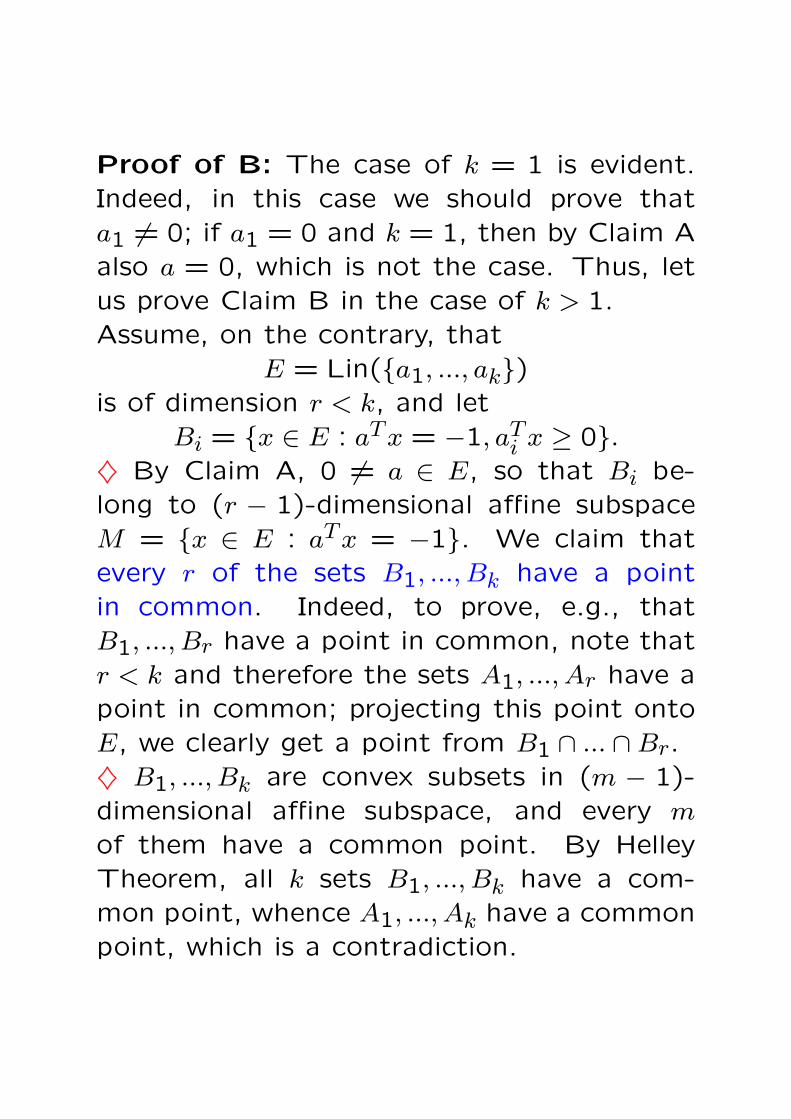
Proof of B: The case of k = 1 is evident.Indeed, in this case we should prove thata1 6= 0; if a1 = 0 and k = 1, then by Claim Aalso a = 0, which is not the case. Thus, letus prove Claim B in the case of k > 1.Assume, on the contrary, that
E = Lin(a1, ..., ak)is of dimension r < k, and let
Bi = x ∈ E : aTx = −1, aTi x ≥ 0.
♦ By Claim A, 0 6= a ∈ E, so that Bi be-long to (r − 1)-dimensional affine subspaceM = x ∈ E : aTx = −1. We claim thatevery r of the sets B1, ..., Bk have a pointin common. Indeed, to prove, e.g., thatB1, ..., Br have a point in common, note thatr < k and therefore the sets A1, ..., Ar have apoint in common; projecting this point ontoE, we clearly get a point from B1 ∩ ... ∩Br.♦ B1, ..., Bk are convex subsets in (m − 1)-dimensional affine subspace, and every m
of them have a common point. By HelleyTheorem, all k sets B1, ..., Bk have a com-mon point, whence A1, ..., Ak have a commonpoint, which is a contradiction.
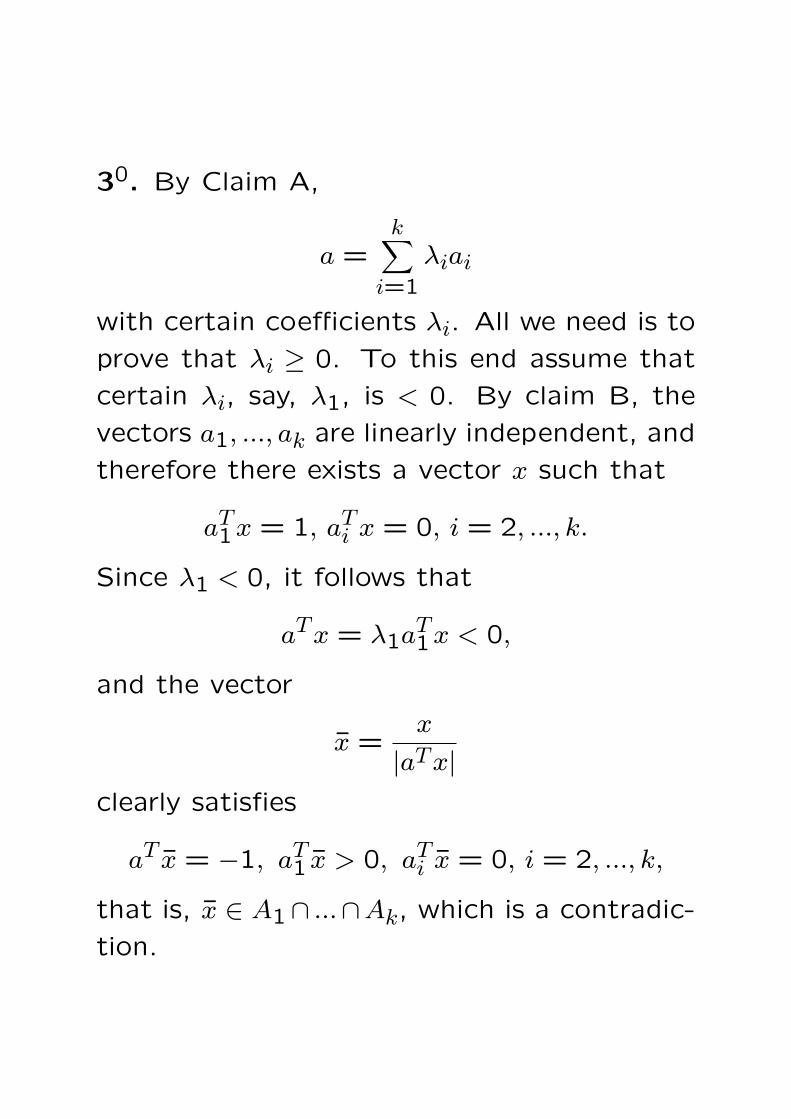
30. By Claim A,
a =k∑
i=1
λiai
with certain coefficients λi. All we need is to
prove that λi ≥ 0. To this end assume that
certain λi, say, λ1, is < 0. By claim B, the
vectors a1, ..., ak are linearly independent, and
therefore there exists a vector x such that
aT1x = 1, aT
i x = 0, i = 2, ..., k.
Since λ1 < 0, it follows that
aTx = λ1aT1x < 0,
and the vector
x =x
|aTx|clearly satisfies
aT x = −1, aT1 x > 0, aT
i x = 0, i = 2, ..., k,
that is, x ∈ A1∩ ...∩Ak, which is a contradic-
tion.

Theory of Systems of Linear Inequalities, II
Theorem on Alternative
♣ A general (finite!) system of linear inequal-
ities with unknowns x ∈ Rn can be written
down as
aTi x > bi, i = 1, ..., ms
aTi x ≥ bi, i = ms + 1, ..., m
(S)
Question: How to certify that (S) is solvable?
Answer: A solution is a certificate of solvabil-
ity!
Question: How to certify that S is not solv-
able?
Answer: ???

aTi x > bi, i = 1, ..., ms
aTi x ≥ bi, i = ms + 1, ..., m
(S)
Question: How to certify that S is not solv-
able?
Conceptual sufficient insolvability condition:
If we can lead the assumption that x solves
(S) to a contradiction, then (S) has no solu-
tions.
“Contradiction by linear aggregation”: Let us
associate with inequalities of (S) nonnegative
weights λi and sum up the inequalities with
these weights. The resulting inequality
m∑
i=1
λiai
T
x
>∑i
λibi,ms∑i=1
λs > 0
≥ ∑i
λibi,ms∑i=1
λs = 0(C)
by its origin is a consequence of (S), that is,
it is satisfied at every solution to (S).
Consequently, if there exist λ ≥ 0 such that
(C) has no solutions at all, then (S) has no
solutions!

Question: When a linear inequality
dTx
>≥ e
has no solutions at all?
Answer: This is the case if and only if d = 0
and
— either the sign is ”>”, and e ≥ 0,
— or the sign is ”≥”, and e > 0.
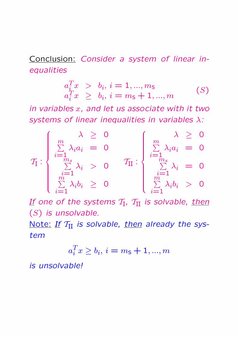
Conclusion: Consider a system of linear in-
equalities
aTi x > bi, i = 1, ..., ms
aTi x ≥ bi, i = ms + 1, ..., m
(S)
in variables x, and let us associate with it two
systems of linear inequalities in variables λ:
TI :
λ ≥ 0m∑
i=1λiai = 0
ms∑i=1
λi > 0
m∑i=1
λibi ≥ 0
TII :
λ ≥ 0m∑
i=1λiai = 0
ms∑i=1
λi = 0
m∑i=1
λibi > 0
If one of the systems TI, TII is solvable, then
(S) is unsolvable.
Note: If TII is solvable, then already the sys-
tem
aTi x ≥ bi, i = ms + 1, ..., m
is unsolvable!

General Theorem on Alternative: A system
of linear inequalities
aTi x > bi, i = 1, ..., ms
aTi x ≥ bi, i = ms + 1, ..., m
(S)
is unsolvable iff one of the systems
TI :
λ ≥ 0m∑
i=1λiai = 0
ms∑i=1
λi > 0
m∑i=1
λibi ≥ 0
TII :
λ ≥ 0m∑
i=1λiai = 0
ms∑i=1
λi = 0
m∑i=1
λibi > 0
is solvable.
Note: The subsystem
aTi x ≥ bi, i = ms + 1, ..., m
of (S) is unsolvable iff TII is solvable!

Proof. We already know that solvability of
one of the systems TI, TII is a sufficient con-
dition for unsolvability of (S). All we need to
prove is that if (S) is unsolvable, then one of
the systems TI, TII is solvable.
Assume that the system
aTi x > bi, i = 1, ..., ms
aTi x ≥ bi, i = ms + 1, ..., m
(S)
in variables x has no solutions. Then every
solution x, τ, ε to the homogeneous system of
inequalities
τ −ε ≥ 0aT
i x −biτ −ε ≥ 0, i = 1, ..., ms
aTi x −biτ ≥ 0, i = ms + 1, ..., m
has ε ≤ 0.
Indeed, in a solution with ε > 0 one would
also have τ > 0, and the vector τ−1x would
solve (S).
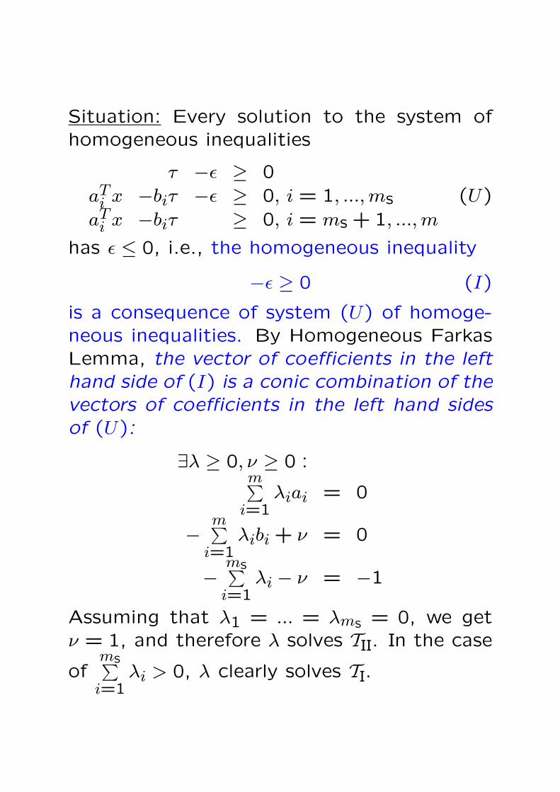
Situation: Every solution to the system ofhomogeneous inequalities
τ −ε ≥ 0aT
i x −biτ −ε ≥ 0, i = 1, ..., ms
aTi x −biτ ≥ 0, i = ms + 1, ..., m
(U)
has ε ≤ 0, i.e., the homogeneous inequality
−ε ≥ 0 (I)
is a consequence of system (U) of homoge-neous inequalities. By Homogeneous FarkasLemma, the vector of coefficients in the lefthand side of (I) is a conic combination of thevectors of coefficients in the left hand sidesof (U):
∃λ ≥ 0, ν ≥ 0 :m∑
i=1λiai = 0
−m∑
i=1λibi + ν = 0
−ms∑i=1
λi − ν = −1
Assuming that λ1 = ... = λms = 0, we getν = 1, and therefore λ solves TII. In the case
ofms∑i=1
λi > 0, λ clearly solves TI.

Corollaries of GTA
♣ Principle A: A finite system of linear in-
equalities has no solutions iff one can lead
it to a contradiction by linear aggregation,
i.e., an appropriate weighted sum of the in-
equalities with “legitimate” weights is either
a contradictory inequality
0Tx > a [a ≥ 0]
or a contradictory inequality
0Tx ≥ a [a > 0]
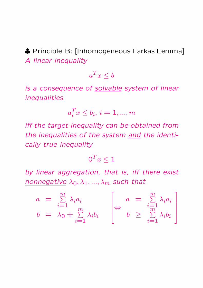
♣ Principle B: [Inhomogeneous Farkas Lemma]
A linear inequality
aTx ≤ b
is a consequence of solvable system of linear
inequalities
aTi x ≤ bi, i = 1, ..., m
iff the target inequality can be obtained from
the inequalities of the system and the identi-
cally true inequality
0Tx ≤ 1
by linear aggregation, that is, iff there exist
nonnegative λ0, λ1, ..., λm such that
a =m∑
i=1λiai
b = λ0 +m∑
i=1λibi
⇔
a =m∑
i=1λiai
b ≥m∑
i=1λibi
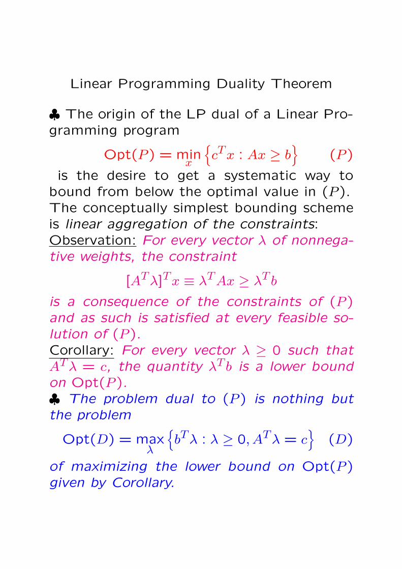
Linear Programming Duality Theorem
♣ The origin of the LP dual of a Linear Pro-gramming program
Opt(P ) = minx
cTx : Ax ≥ b
(P )
is the desire to get a systematic way tobound from below the optimal value in (P ).The conceptually simplest bounding schemeis linear aggregation of the constraints:Observation: For every vector λ of nonnega-tive weights, the constraint
[ATλ]Tx ≡ λTAx ≥ λT b
is a consequence of the constraints of (P )and as such is satisfied at every feasible so-lution of (P ).Corollary: For every vector λ ≥ 0 such thatATλ = c, the quantity λT b is a lower boundon Opt(P ).♣ The problem dual to (P ) is nothing butthe problem
Opt(D) = maxλ
bTλ : λ ≥ 0, ATλ = c
(D)
of maximizing the lower bound on Opt(P )given by Corollary.
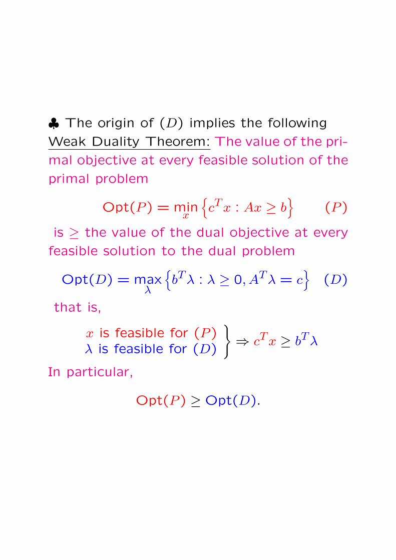
♣ The origin of (D) implies the following
Weak Duality Theorem: The value of the pri-
mal objective at every feasible solution of the
primal problem
Opt(P ) = minx
cTx : Ax ≥ b
(P )
is ≥ the value of the dual objective at every
feasible solution to the dual problem
Opt(D) = maxλ
bTλ : λ ≥ 0, ATλ = c
(D)
that is,
x is feasible for (P )λ is feasible for (D)
⇒ cTx ≥ bTλ
In particular,
Opt(P ) ≥ Opt(D).
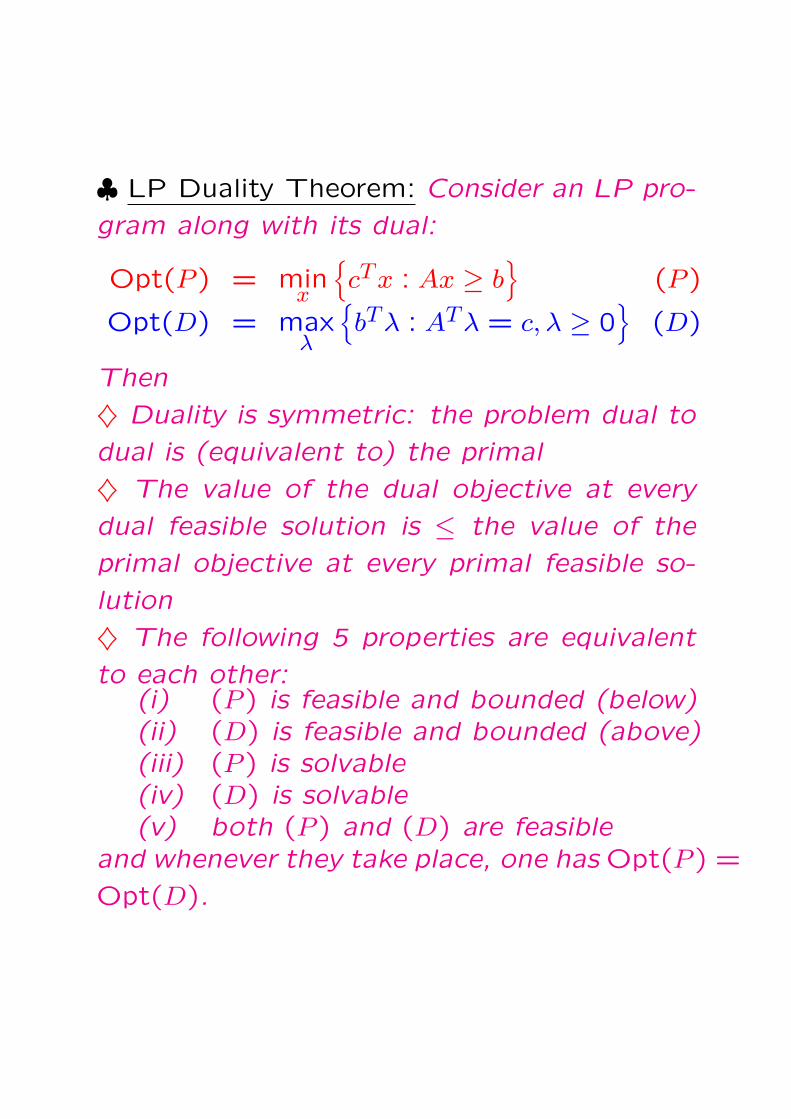
♣ LP Duality Theorem: Consider an LP pro-
gram along with its dual:
Opt(P ) = minx
cTx : Ax ≥ b
(P )
Opt(D) = maxλ
bTλ : ATλ = c, λ ≥ 0
(D)
Then
♦ Duality is symmetric: the problem dual to
dual is (equivalent to) the primal
♦ The value of the dual objective at every
dual feasible solution is ≤ the value of the
primal objective at every primal feasible so-
lution
♦ The following 5 properties are equivalent
to each other:(i) (P ) is feasible and bounded (below)(ii) (D) is feasible and bounded (above)(iii) (P ) is solvable(iv) (D) is solvable(v) both (P ) and (D) are feasible
and whenever they take place, one has Opt(P ) =
Opt(D).
Opt(P ) = minx
cTx : Ax ≥ b
(P )
Opt(D) = maxλ
bTλ : ATλ = c, λ ≥ 0
(D)
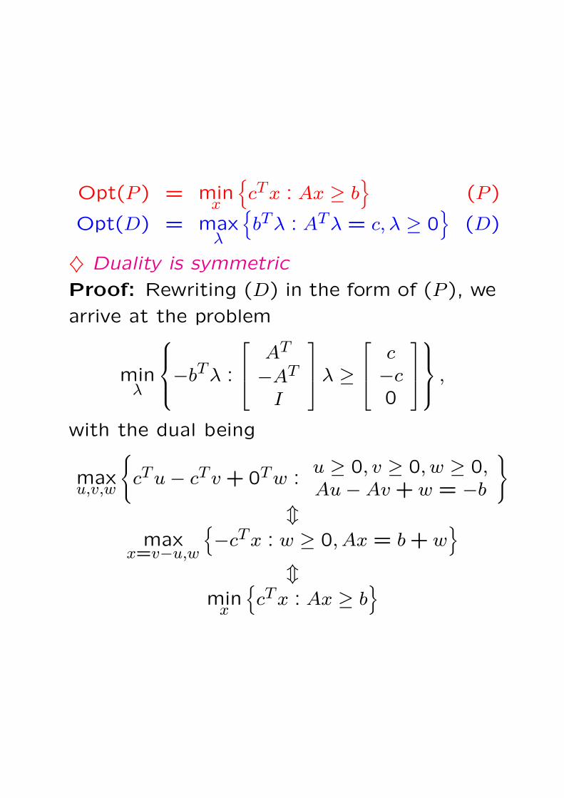
♦ Duality is symmetric
Proof: Rewriting (D) in the form of (P ), we
arrive at the problem
minλ
−bTλ :
AT
−AT
I
λ ≥
c−c0
,
with the dual being
maxu,v,w
cTu− cTv + 0Tw :
u ≥ 0, v ≥ 0, w ≥ 0,Au−Av + w = −b
mmax
x=v−u,w
−cTx : w ≥ 0, Ax = b + w
mmin
x
cTx : Ax ≥ b

♦ The value of the dual objective at every
dual feasible solution is ≤ the value of the
primal objective at every primal feasible so-
lution
This is Weak Duality
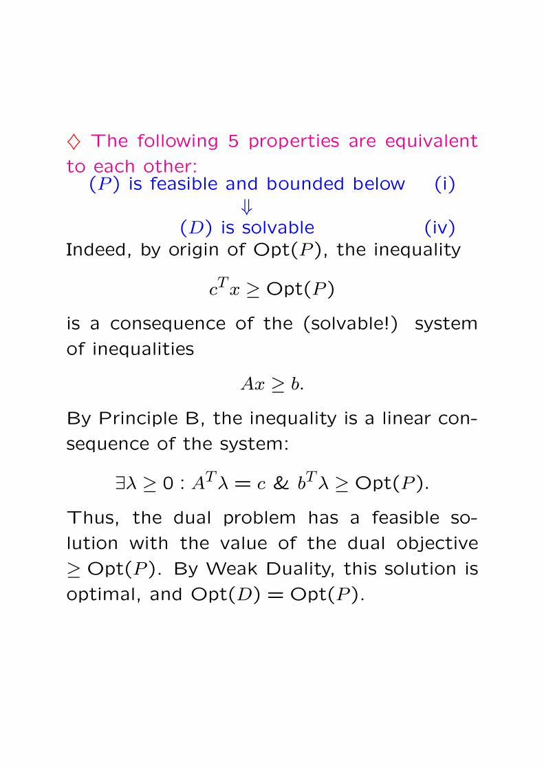
♦ The following 5 properties are equivalent
to each other:(P ) is feasible and bounded below (i)
⇓(D) is solvable (iv)
Indeed, by origin of Opt(P ), the inequality
cTx ≥ Opt(P )
is a consequence of the (solvable!) system
of inequalities
Ax ≥ b.
By Principle B, the inequality is a linear con-
sequence of the system:
∃λ ≥ 0 : ATλ = c & bTλ ≥ Opt(P ).
Thus, the dual problem has a feasible so-
lution with the value of the dual objective
≥ Opt(P ). By Weak Duality, this solution is
optimal, and Opt(D) = Opt(P ).

♦ The following 5 properties are equivalent
to each other:(D) is solvable (iv)
⇓(D) is feasible and bounded above (ii)
Evident
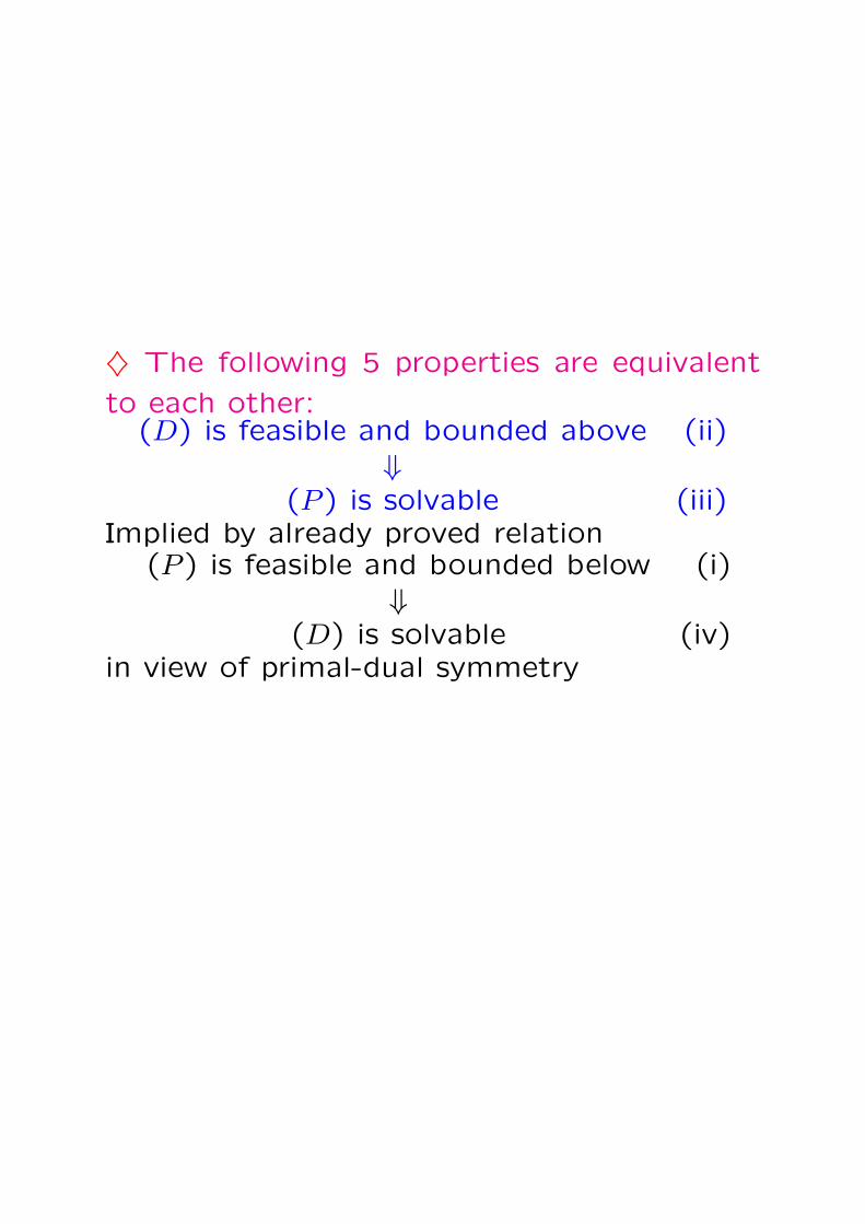
♦ The following 5 properties are equivalent
to each other:(D) is feasible and bounded above (ii)
⇓(P ) is solvable (iii)
Implied by already proved relation(P ) is feasible and bounded below (i)
⇓(D) is solvable (iv)
in view of primal-dual symmetry

♦ The following 5 properties are equivalent
to each other:(P ) is solvable (iii)
⇓(P ) is feasible and bounded below (i)
Evident

We proved that
(i) ⇔ (ii) ⇔ (iii) ⇔ (iv)
and that when these 4 equivalent properties
take place, one has
Opt(P ) = Opt(D)
It remains to prove that properties (i) – (iv)
are equivalent to
both (P ) and (D) are feasible (v)
♦ In the case of (v), (P ) is feasible and below
bounded (Weak Duality), so that (v)⇒(i)
♦ in the case of (i)≡(ii), both (P ) and (D)
are feasible, so that (i)⇒(v)
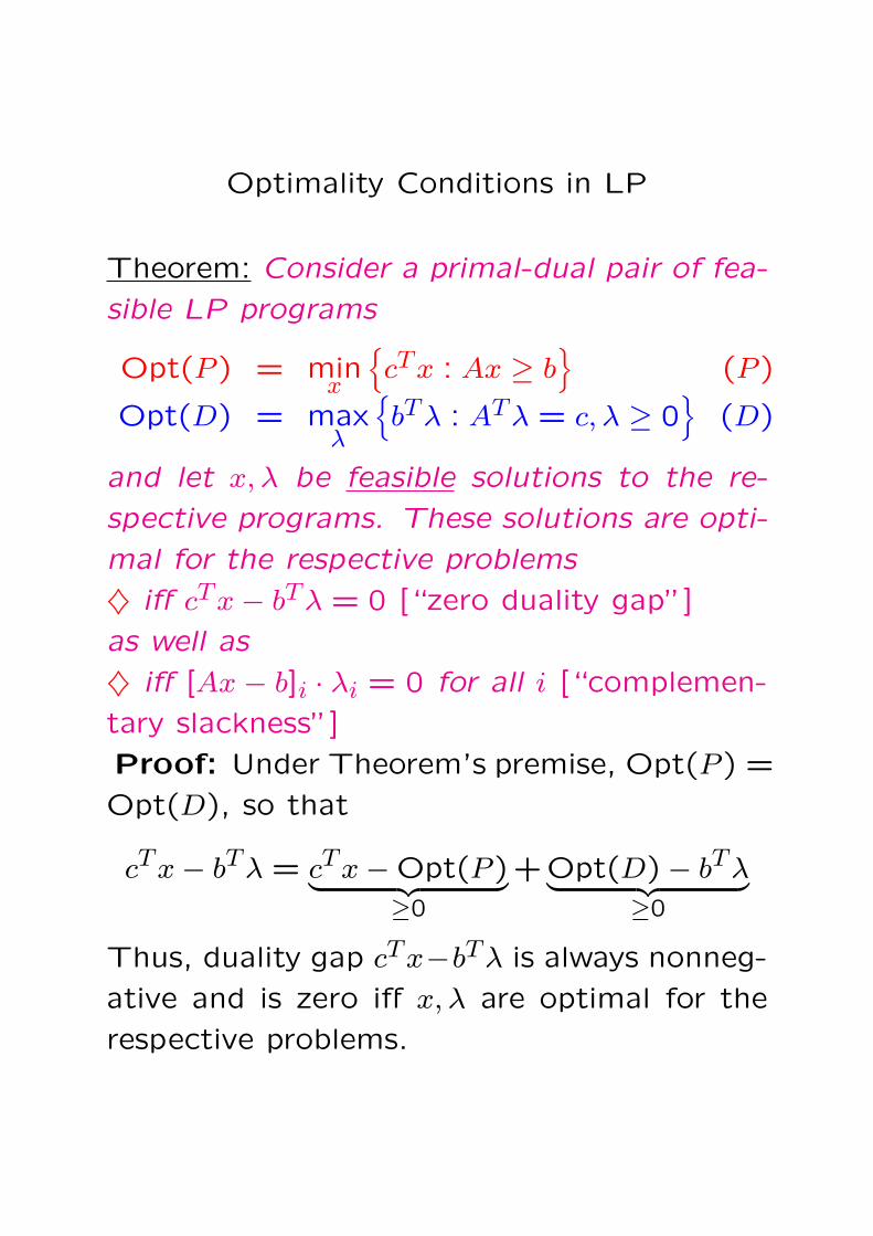
Optimality Conditions in LP
Theorem: Consider a primal-dual pair of fea-
sible LP programs
Opt(P ) = minx
cTx : Ax ≥ b
(P )
Opt(D) = maxλ
bTλ : ATλ = c, λ ≥ 0
(D)
and let x, λ be feasible solutions to the re-
spective programs. These solutions are opti-
mal for the respective problems
♦ iff cTx− bTλ = 0 [“zero duality gap”]
as well as
♦ iff [Ax − b]i · λi = 0 for all i [“complemen-
tary slackness”]
Proof: Under Theorem’s premise, Opt(P ) =
Opt(D), so that
cTx− bTλ = cTx−Opt(P )︸ ︷︷ ︸≥0
+Opt(D)− bTλ︸ ︷︷ ︸≥0
Thus, duality gap cTx−bTλ is always nonneg-
ative and is zero iff x, λ are optimal for the
respective problems.

The complementary slackness condition is
given by the identity
cTx− bTλ = (ATλ)Tx− bTλ = [Ax− b]Tλ
Since both [Ax−b] and λ are nonnegative, du-
ality gap is zero iff the complementary slack-
ness holds true.

Separation Theorem
♣ Every linear form f(x) on Rn is repre-
sentable via inner product:
f(x) = fTx
for appropriate vector f ∈ Rn uniquely defined
by the form. Nontrivial (not identically zero)
forms correspond to nonzero vectors f .
♣ A level set
M =x : fTx = a
(∗)
of a nontrivial linear form on Rn is affine sub-
space of affine dimension n − 1; vice versa,
every affine subspace M of affine dimension
n − 1 in Rn can be represented by (∗) with
appropriately chosen f 6= 0 and a; f and a
are defined by M up to multiplication by a
common nonzero factor.
(n−1)-dimensional affine subspaces in Rn are
called hyperplanes.
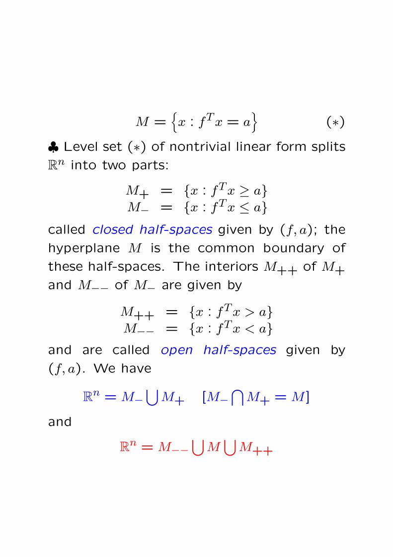
M =x : fTx = a
(∗)
♣ Level set (∗) of nontrivial linear form splits
Rn into two parts:
M+ = x : fTx ≥ aM− = x : fTx ≤ a
called closed half-spaces given by (f, a); the
hyperplane M is the common boundary of
these half-spaces. The interiors M++ of M+
and M−− of M− are given by
M++ = x : fTx > aM−− = x : fTx < a
and are called open half-spaces given by
(f, a). We have
Rn = M−⋃
M+ [M−⋂
M+ = M ]
and
Rn = M−−⋃
M⋃
M++
♣ Definition. Let T, S be two nonempty sets
in Rn.
(i) We say that a hyperplane
M = x : fTx = a (∗)separates S and T , if
♦ S ⊂ M−, T ⊂ M+ (“S does not go above
M , and T does not go below M”)
and
♦ S ∪ T 6⊂ M .
(ii) We say that a nontrivial linear form fTx
separates S and T if, for properly chosen a,
the hyperplane (∗) separates S and T .
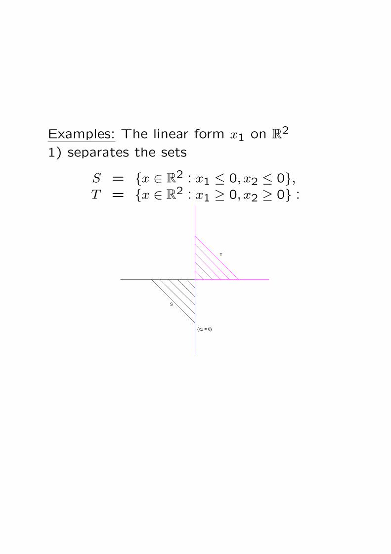
Examples: The linear form x1 on R2
1) separates the sets
S = x ∈ R2 : x1 ≤ 0, x2 ≤ 0,T = x ∈ R2 : x1 ≥ 0, x2 ≥ 0 :
T
S
x1 = 0

2) separates the sets
S = x ∈ R2 : x1 ≤ 0, x2 ≤ 0,T = x ∈ R2 : x1 + x2 ≥ 0, x2 ≤ 0 :
TS
x1 = 0

3) does not separate the sets
S = x ∈ R2 : x1 = 0,1 ≤ x2 ≤ 2,T = x ∈ R2 : x1 = 0,−2 ≤ x2 ≤ −1 :
S
T
x1 = 0
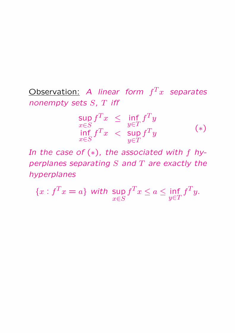
Observation: A linear form fTx separates
nonempty sets S, T iff
supx∈S
fTx ≤ infy∈T
fTy
infx∈S
fTx < supy∈T
fTy(∗)
In the case of (∗), the associated with f hy-
perplanes separating S and T are exactly the
hyperplanes
x : fTx = a with supx∈S
fTx ≤ a ≤ infy∈T
fTy.

♣ Separation Theorem: Two nonempty convex
sets S, T can be separated iff their relative
interiors do not intersect.
Note: In this statement, convexity of both S
and T is crucial!
S T

Proof, ⇒: (!) If nonempty convex sets S, T
can be separated, then rint S⋂
rint T = ∅Lemma. Let X be a convex set, f(x) = fTx
be a linear form and a ∈ rint X. Then
fTa = maxx∈X
fTx ⇔ f(·)∣∣∣∣∣X
= const.
♣ Lemma ⇒ (!): Let a ∈ rint S ∩ rint T . As-sume, on contrary to what should be proved,that fTx separates S, T , so that
supx∈S
fTx ≤ infy∈T
fTy.
♦ Since a ∈ T , we get fTa ≥ supx∈S
fTx, that is,
fTa = maxx∈S
fTx. By Lemma, fTx = fTa for
all x ∈ S.♦ Since a ∈ S, we get fTa ≤ inf
y∈TfTy, that is,
fTa = miny∈T
fTy. By Lemma, fTy = fTa for
all y ∈ T .Thus,
z ∈ S ∪ T ⇒ fT z ≡ fTa,
so that f does not separate S and T , whichis a contradiction.

Lemma. Let X be a convex set, f(x) = fTx
be a linear form and a ∈ rint X. Then
fTa = maxx∈X
fTx ⇔ f(·)∣∣∣∣∣X
= const.
Proof. Shifting X, we may assume a = 0.
Let, on the contrary to what should be
proved, fTx be non-constant on X, so that
there exists y ∈ X with fTy 6= fTa = 0. The
case of fTy > 0 is impossible, since fTa = 0
is the maximum of fTx on X. Thus, fTy < 0.
The line ty : t ∈ R passing through 0 and
through y belongs to Aff(X); since 0 ∈ rint X,
all points z = −εy on this line belong to X,
provided that ε > 0 is small enough. At every
point of this type, fT z > 0, which contradicts
the fact that maxx∈X
fTx = fTa = 0.

Proof, ⇐: Assume that S, T are nonempty
convex sets such that rint S ∩ rint T = ∅, and
let us prove that S, T can be separated.
Step 1: Separating a point and a convex
hull of a finite set. Let S = Conv(b1, ..., bm)and T = b with b 6∈ S, and let us prove that
S and T can be separated.
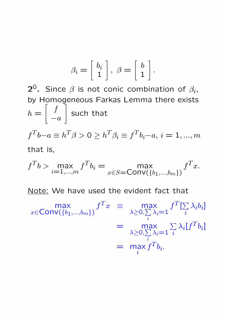
10. Let
βi =
[bi1
], β =
[b1
].
Observe that β is not a conic combination of
β1, ..., βm:[
b1
]=
m∑i=1
λi
[bi1
], λi ≥ 0
⇓b =
∑i
λibi,∑i
λi = 1, λi ≥ 0
⇓b ∈ S – contradiction!
βi =
[bi1
], β =
[b1
].
20. Since β is not conic combination of βi,
by Homogeneous Farkas Lemma there exists
h =
[f−a
]such that
fT b−a ≡ hTβ > 0 ≥ hTβi ≡ fT bi−a, i = 1, ..., m
that is,
fT b > maxi=1,...,m
fT bi = maxx∈S=Conv(b1,...,bm)
fTx.
Note: We have used the evident fact that
maxx∈Conv(b1,...,bm)
fTx ≡ maxλ≥0,
∑i
λi=1fT [
∑i
λibi]
= maxλ≥0,
∑i
λi=1
∑i
λi[fT bi]
= maxi
fT bi.
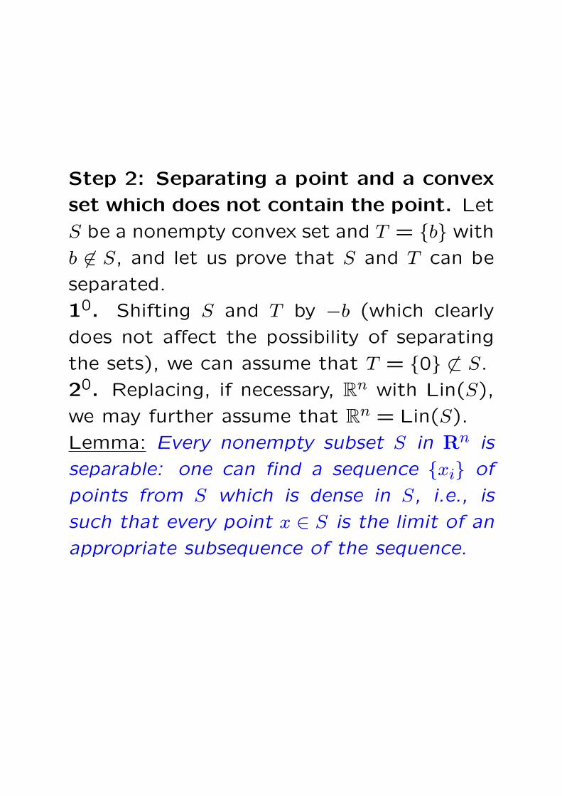
Step 2: Separating a point and a convex
set which does not contain the point. Let
S be a nonempty convex set and T = b with
b 6∈ S, and let us prove that S and T can be
separated.
10. Shifting S and T by −b (which clearly
does not affect the possibility of separating
the sets), we can assume that T = 0 6⊂ S.
20. Replacing, if necessary, Rn with Lin(S),
we may further assume that Rn = Lin(S).
Lemma: Every nonempty subset S in Rn is
separable: one can find a sequence xi of
points from S which is dense in S, i.e., is
such that every point x ∈ S is the limit of an
appropriate subsequence of the sequence.

Lemma ⇒ Separation: Let xi ∈ S be a
sequence which is dense in S. Since S is
convex and does not contain 0, we have
0 6∈ Conv(x1, ..., xi) ∀iwhence
∃fi : 0 = fTi 0 > max
1≤j≤ifTi xj. (∗)
By scaling, we may assume that ‖fi‖2 = 1.
The sequence fi of unit vectors possesses
a converging subsequence fis∞s=1; the limit
f of this subsequence is, of course, a unit
vector. By (∗), for every fixed j and all large
enough s we have fTis
xj < 0, whence
fTxj ≤ 0 ∀j. (∗∗)Since xj is dense in S, (∗∗) implies that
fTx ≤ 0 for all x ∈ S, whence
supx∈S
fTx ≤ 0 = fT0.
Situation: (a) Lin(S) = Rn
(b) T = 0(c) We have built a unit vector f such that
supx∈S
fTx ≤ 0 = fT0. (!)
By (!), all we need to prove that f separates
T = 0 and S is to verify that
infx∈S
fTx < fT0 = 0.
Assuming the opposite, (!) would say that
fTx = 0 for all x ∈ S, which is impossible,
since Lin(S) = Rn and f is nonzero.
Lemma: Every nonempty subset S in Rn is
separable: one can find a sequence xi of
points from S which is dense in S, i.e., is
such that every point x ∈ S is the limit of an
appropriate subsequence of the sequence.
Proof. Let r1, r2, ... be the countable set of
all rational vectors in Rn. For every positive
integer t, let Xt ⊂ S be the countable set
given by the following construction:
We look, one after another, at the
points r1, r2, ... and for every point rs
check whether there is a point z in S
which is at most at the distance 1/t
away from rs. If points z with this
property exist, we take one of them
and add it to Xt and then pass to
rs+1, otherwise directly pass to rs+1.

Is is clear that
(*) Every point x ∈ S is at the dis-
tance at most 2/t from certain point
of Xt.
Indeed, since the rational vectors are dense
in Rn, there exists s such that rs is at the
distance ≤ 1t from x. Therefore, when pro-
cessing rs, we definitely add to Xt a point z
which is at the distance ≤ 1/t from rs and
thus is at the distance ≤ 2/t from x.
By construction, the countable union∞⋃
t=1Xt
of countable sets Xt ⊂ S is a countable set
in S, and by (*) this set is dense in S.

Step 3: Separating two non-intersecting
nonempty convex sets. Let S, T be
nonempty convex sets which do not inter-
sect; let us prove that S, T can be separated.
Let S = S − T and T = 0. The set
S clearly is convex and does not contain 0
(since S ∩ T = ∅). By Step 2, S and 0 = T
can be separated: there exists f such that
supx∈S
fT s− infy∈T
fT y
︷ ︸︸ ︷sup
x∈S,y∈T[fTx− fTy] ≤ 0 = inf
z∈0fTz
infx∈S,y∈T
[fTx− fTy]︸ ︷︷ ︸
infx∈S
fT x−supy∈T
fT y
< 0 = supz∈0
fTz
whence
supx∈S
fTx ≤ infy∈T
fTy
infx∈S
fTx < supy∈T
fTy

Step 4: Completing the proof of Sep-
aration Theorem. Finally, let S, T be
nonempty convex sets with non-intersecting
relative interiors, and let us prove that S, T
can be separated.
As we know, the sets S′ = rint S and T ′ =
rint T are convex and nonempty; we are in
the situation when these sets do not inter-
sect. By Step 3, S′ and T ′ can be separated:
for properly chosen f , one has
supx∈S′
fTx ≤ infy∈T ′
fTy
infx∈S′
fTx < supy∈T ′
fTy(∗)
Since S′ is dense in S and T ′ is dense in T ,
inf’s and sup’s in (∗) remain the same when
replacing S′ with S and T ′ with T . Thus, f
separates S and T .

♣ Alternative proof of Separation Theorem
starts with separating a point T = a and a
closed convex set S, a 6∈ S, and is based on
the following fact:
Let S be a nonempty closed convex
set and let a 6∈ S. There exists a
unique closest to a point in S:
ProjS(a) = argminx∈S
‖a− x‖2
and the vector e = a−ProjS(a) sepa-
rates a and S:
maxx∈S
eTx = eTProjS(a) = eTa−‖e‖22 < eTa.

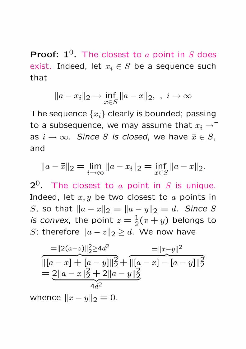
Proof: 10. The closest to a point in S does
exist. Indeed, let xi ∈ S be a sequence such
that
‖a− xi‖2 → infx∈S
‖a− x‖2, , i →∞
The sequence xi clearly is bounded; passing
to a subsequence, we may assume that xi →¯
as i → ∞. Since S is closed, we have x ∈ S,
and
‖a− x‖2 = limi→∞ ‖a− xi‖2 = inf
x∈S‖a− x‖2.
20. The closest to a point in S is unique.
Indeed, let x, y be two closest to a points in
S, so that ‖a − x‖2 = ‖a − y‖2 = d. Since S
is convex, the point z = 12(x + y) belongs to
S; therefore ‖a− z‖2 ≥ d. We now have
=‖2(a−z)‖22≥4d2
︷ ︸︸ ︷‖[a− x] + [a− y]‖22 +
=‖x−y‖2︷ ︸︸ ︷‖[a− x]− [a− y]‖22
= 2‖a− x‖22 + 2‖a− y‖22︸ ︷︷ ︸4d2
whence ‖x− y‖2 = 0.
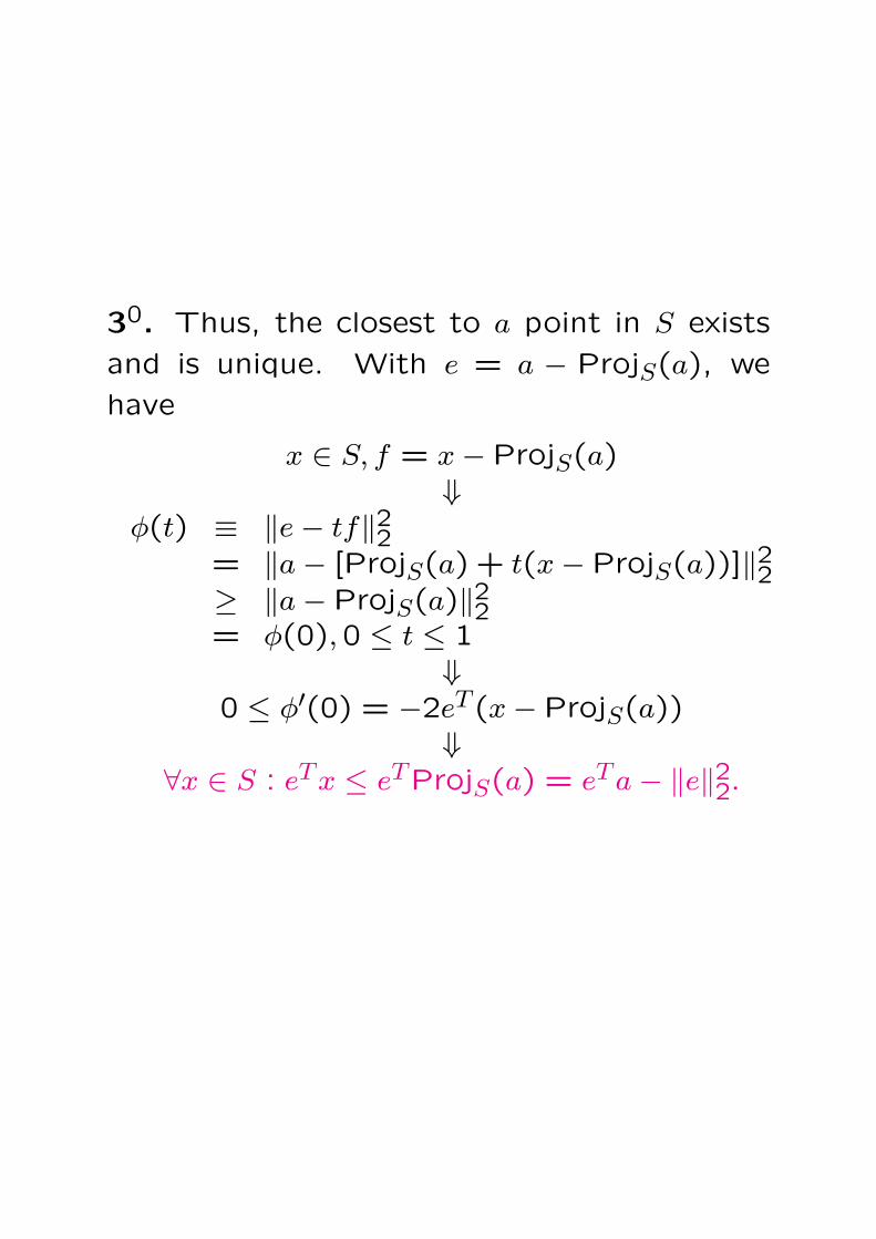
30. Thus, the closest to a point in S exists
and is unique. With e = a − ProjS(a), we
have
x ∈ S, f = x− ProjS(a)⇓
φ(t) ≡ ‖e− tf‖22= ‖a− [ProjS(a) + t(x− ProjS(a))]‖22≥ ‖a− ProjS(a)‖22= φ(0),0 ≤ t ≤ 1
⇓0 ≤ φ′(0) = −2eT (x− ProjS(a))
⇓∀x ∈ S : eTx ≤ eTProjS(a) = eTa− ‖e‖22.
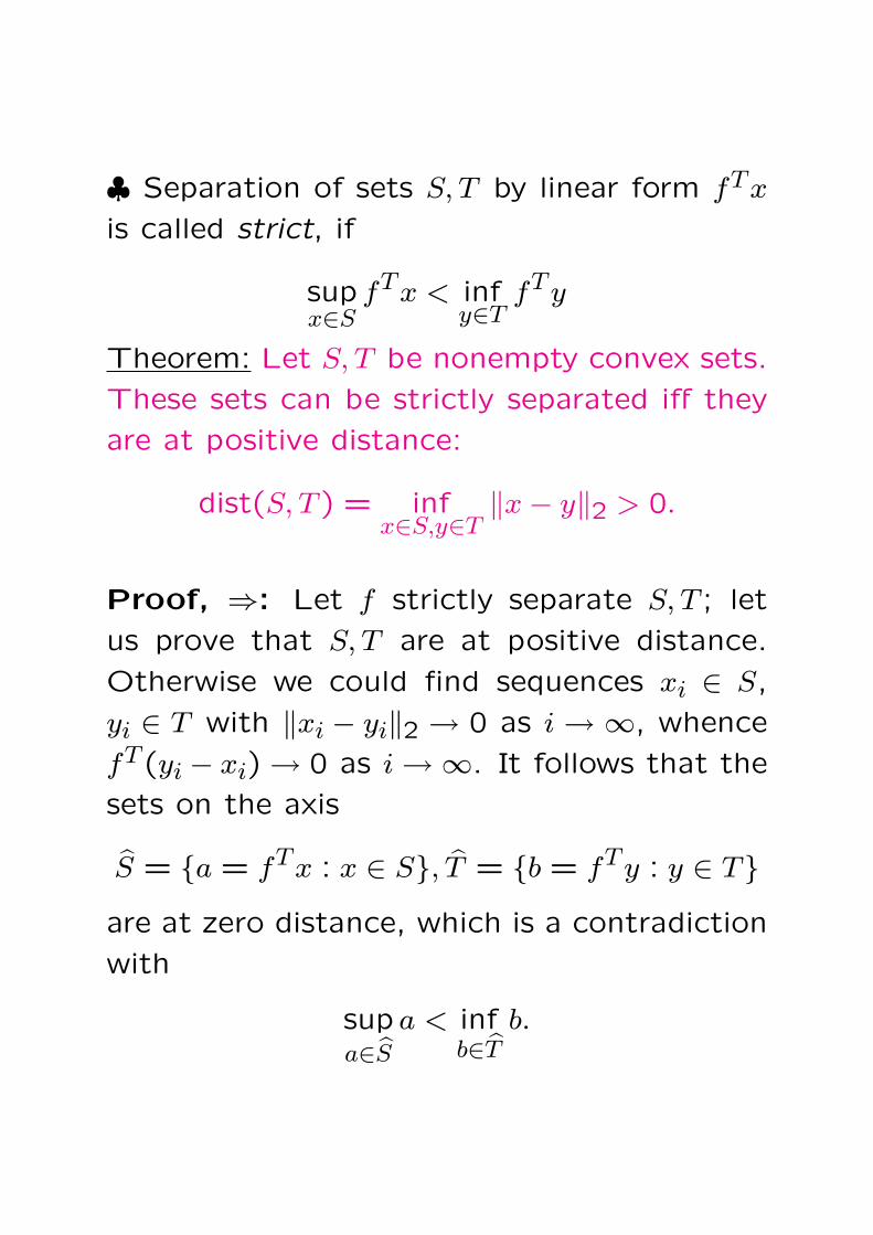
♣ Separation of sets S, T by linear form fTx
is called strict, if
supx∈S
fTx < infy∈T
fTy
Theorem: Let S, T be nonempty convex sets.
These sets can be strictly separated iff they
are at positive distance:
dist(S, T ) = infx∈S,y∈T
‖x− y‖2 > 0.
Proof, ⇒: Let f strictly separate S, T ; let
us prove that S, T are at positive distance.
Otherwise we could find sequences xi ∈ S,
yi ∈ T with ‖xi − yi‖2 → 0 as i → ∞, whence
fT (yi − xi) → 0 as i →∞. It follows that the
sets on the axis
S = a = fTx : x ∈ S, T = b = fTy : y ∈ Tare at zero distance, which is a contradiction
with
supa∈S
a < infb∈T
b.

Proof, ⇐: Let T , S be nonempty convex
sets which are at positive distance 2δ:
2δ = infx∈S,y∈T
‖x− y‖2 > 0.
Let
S+ = S + z : ‖z‖2 ≤ δThe sets S+ and T are convex and do not
intersect, and thus can be separated:
supx+∈S+
fTx+ ≤ infy∈T
fTy [f 6= 0]
Since
supx+∈S+
fTx+ = supx∈S,‖z‖2≤δ
[fTx + fT z]
= [supx∈S
fTx] + δ‖f‖2,
we arrive at
supx∈S
fTx < infy∈T
fTy
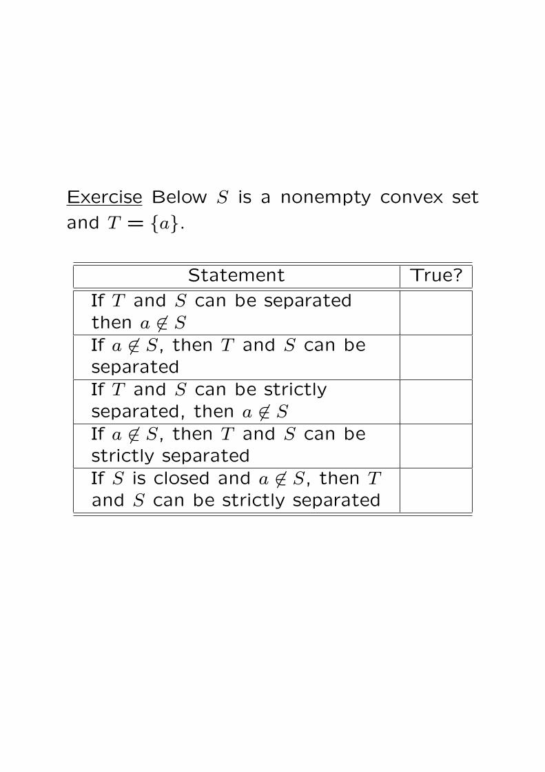
Exercise Below S is a nonempty convex set
and T = a.
Statement True?
If T and S can be separatedthen a 6∈ SIf a 6∈ S, then T and S can beseparatedIf T and S can be strictlyseparated, then a 6∈ SIf a 6∈ S, then T and S can bestrictly separatedIf S is closed and a 6∈ S, then Tand S can be strictly separated
Supporting Planes and Extreme Points
♣ Definition. Let Q be a closed convex set in
Rn and x be a point from the relative bound-
ary of Q. A hyperplane
Π = x : fTx = a [a 6= 0]
is called supporting to Q at the point x, if
the hyperplane separates Q and x:supx∈Q
fTx ≤ fT x
infx∈Q
fTx < f tx
Equivalently: Hyperplane Π = x : fTx = asupports Q at x iff the linear form fTx attains
its maximum on Q, equal to a, at the point
x and the form is non-constant on Q.
Proposition. Let Q be a convex closed set in
Rn and x be a point from the relative bound-
ary of Q. Then
♦ There exist at least one hyperplane Π
which supports Q at x;
♦ For every such hyperplane Π, the set Q∩Π
has dimension less than the one of Q.
Proof: Existence of supporting plane is given
by Separation Theorem. This theorem is ap-
plicable since
x 6∈ rint Q ⇒ x ≡ rint x ∩ rint Q = ∅.Further,
Q * Π ⇒ Aff(Q) * Π ⇒ Aff(Π ∩Q) $ Aff(Q),
and if two distinct affine subspaces are em-
bedded one into another, then the dimension
of the embedded subspace is strictly less than
the dimension of the embedding one.
Extreme Points
♣ Definition. Let Q be a convex set in Rn and
x be a point of X. The point is called ex-
treme, if it is not a convex combination, with
positive weights, of two points of X distinct
from x:
x ∈ Ext(Q)m
x ∈ Q &
u, v ∈ Q, λ ∈ (0,1)x = λu + (1− λ)v
⇒ u = v = x
Equivalently: A point x ∈ Q is extreme iff it
is not the midpoint of a nontrivial segment
in Q:
x± h ∈ Q ⇒ h = 0.
Equivalently: A point x ∈ Q is extreme iff the
set Q\x is convex.

Examples:
1. Extreme points of [x, y] are ...
2. Extreme points of 4ABC are ...
3. Extreme points of the ball x : ‖x‖2 ≤ 1are ...

Theorem [Krein-Milman] Let Q be a closed
convex and nonempty set in Rn. Then
♦ Q possess extreme points iff Q does not
contain lines;
♦ If Q is bounded, then Q is the convex hull
of its extreme points:
Q = Conv(Ext(Q))
so that every point of Q is convex combina-
tion of extreme points of Q.
Note: If Q = Conv(A), then Ext(Q) ⊂ A.
Thus, extreme points of a closed convex
bounded set Q give the minimal representa-
tion of Q as Conv(...).

Proof. 10: If closed convex set Q does not
contain lines, then Ext(Q) 6= ∅Important lemma: Let S be a closed convex
set and Π = x : fTx = a be a hyperplane
which supports S at certain point. Then
Ext(Π ∩ S) ⊂ Ext(S).
Proof of Lemma. Let x ∈ Ext(Π ∩ S);
we should prove that x ∈ Ext(S). Assume,
on the contrary, that x is a midpoint of a
nontrivial segment [u, v] ⊂ S. Then fT x =
a = maxx∈S
fTx, whence fT x = maxx∈[u,v]
fTx. A
linear form can attain its maximum on a
segment at the midpoint of the segment iff
the form is constant on the segment; thus,
a = fT x = fTu = fTv, that is, [u, v] ⊂ Π ∩ S.
But x is an extreme point of Π∩ S – contra-
diction!
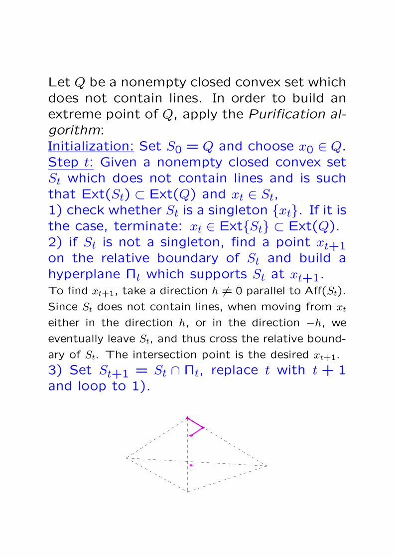
Let Q be a nonempty closed convex set whichdoes not contain lines. In order to build anextreme point of Q, apply the Purification al-gorithm:Initialization: Set S0 = Q and choose x0 ∈ Q.Step t: Given a nonempty closed convex setSt which does not contain lines and is suchthat Ext(St) ⊂ Ext(Q) and xt ∈ St,1) check whether St is a singleton xt. If it isthe case, terminate: xt ∈ ExtSt ⊂ Ext(Q).2) if St is not a singleton, find a point xt+1on the relative boundary of St and build ahyperplane Πt which supports St at xt+1.To find xt+1, take a direction h 6= 0 parallel to Aff(St).
Since St does not contain lines, when moving from xt
either in the direction h, or in the direction −h, we
eventually leave St, and thus cross the relative bound-
ary of St. The intersection point is the desired xt+1.
3) Set St+1 = St ∩ Πt, replace t with t + 1and loop to 1).

Justification: By Important Lemma,
Ext(St+1) ⊂ Ext(St),
so that
Ext(St) ⊂ Ext(Q) ∀t.Besides this, dim (St+1 < dim(St), so that
Purification algorithm does terminate. the
algorithm
Note: Assume you are given a linear form gTx
which is bounded from above on Q. Then
in the Purification algorithm one can easily
ensure that gTxt+1 ≥ gTxt. Thus,
If Q is a nonempty closed set in Rn which
does not contain lines and fTx is a linear form
which is bounded above on Q, then for every
point x0 ∈ Q there exists (and can be found
by Purification) a point x ∈ Ext(Q) such that
gT x ≥ gTx0. In particular, if gTx attains its
maximum on Q, then the maximizer can be
found among extreme points of Q.

Proof, 20 If a closed convex set Q contains
lines, it has no extreme points.
Another Important Lemma: Let S be a closed
convex set such that x + th : t ≥ 0 ⊂ S for
certain x. Then
x + th : t ≥ 0 ⊂ S ∀x ∈ S.
Proof: For every s ≥ 0 and x ∈ S we have
x + sh = limi→∞ [(1− s/i)x + (s/i)[x + th]]︸ ︷︷ ︸
∈S
.
Note: The set of all directions h ∈ Rn such
that x + th : t ≥ 0 ⊂ S for some (and then,
for all) x ∈ S, is called the recessive cone
Rec(S) of closed convex set S. Rec(S) in-
deed is a cone, and
S + Rec(S) = S.
Corollary: If a closed convex set Q contains a
line `, then the parallel lines, passing through
points of Q, also belong to Q. In particular,
Q possesses no extreme points.
Proof, 30: If a nonempty closed convex set
Q is bounded, then Q = Conv(Ext(Q)).
The inclusion Conv(Ext(Q)) ⊂ Q is evident.
Let us prove the opposite inclusion, i.e.,
prove that every point of Q is a convex com-
bination of extreme points of Q.
Induction in k = dimQ. Base k = 0 (Q is a
singleton) is evident.
Step k 7→ k + 1: Given (k + 1)-dimensional
closed and bounded convex set Q and a
point x ∈ Q, we, as in the Purification al-
gorithm, can represent x as a convex com-
bination of two points x+ and x− from the
relative boundary of Q. Let Π+ be a hy-
perplane which supports Q at x+, and let
Q+ = Π+ ∩ Q. As we know, Q+ is a closed
convex set such that
dimQ+ < dimQ, Ext(Q+) ⊂ Ext(Q), x+ ∈ Q+.
Invoking inductive hypothesis,
x+ ∈ Conv(Ext(Q+)) ⊂ Conv(Ext(Q)).
Similarly, x− ∈ Conv(Ext(Q)). Since x ∈[x−, x+], we get x ∈ Conv(Ext(Q)).
Structure of Polyhedral Sets
♣ Definition: A polyhedral set Q in Rn is a
nonempty subset in Rn which is a solution set
of a finite system of nonstrict inequalities:
Q is polyhedral ⇔ Q = x : Ax ≥ b 6= ∅.
♠ Every polyhedral set is convex and closed.
Question: When a polyhedral set Q = x :Ax ≥ b contains lines? What are these lines,if any?Answer: Q contains lines iff A has a nontrivialnullspace:
Null(A) ≡ h : Ah = 0 6= 0.
Indeed, a line ` = x = x + th : t ∈ R, h 6= 0,belongs to Q iff
∀t : A(x + th) ≥ b⇔ ∀t : tAh ≥ b−Ax⇔ Ah = 0 & x ∈ Q.
Fact: A polyhedral set Q = x : Ax ≥ b al-ways can be represented as
Q = Q∗ + L,
where Q∗ is a polyhedral set which does notcontain lines and L is a linear subspace. Inthis representation,♦ L is uniquely defined by Q and coincideswith Null(A),♦ Q∗ can be chosen, e.g., as
Q∗ = Q ∩ L⊥
Structure of polyhedral set which does not
contain lines
♣ Theorem. Let
Q = x : Ax ≥ b 6= ∅be a polyhedral set which does not contain
lines (or, which is the same, Null(A) = 0).Then the set Ext(Q) of extreme points of Q
is nonempty and finite, and
Q = Conv(Ext(Q)) + Cone r1, ..., rS (∗)for properly chosen vectors r1, ..., rS.
Note: Cone r1, ..., rs is exactly the recessive
cone of Q:
Cone r1, ..., rS= r : x + tr ∈ Q ∀(x ∈ Q, t ≥ 0)= r : Ar ≥ 0.
This cone is the trivial cone 0 iff Q is a
bounded polyhedral set (called polytope).

♣ Combining the above theorems, we come
to the following results:
A polyhedral set Q always can be represented
in the form
Q =
x =
I∑
i=1
λivi +J∑
j=1
µjwj :λ ≥ 0, µ ≥ 0∑i
λi = 1
(!)
where I, J are positive integers and v1, ..., vI,
w1, ..., wJ are appropriately chosen points and
directions.
Vice versa, every set Q of the form (!) is a
polyhedral set.
Note: Polytopes (bounded polyhedral sets)
are exactly the sets of form (!) with “trivial
w-part”: w1 = ... = wJ = 0.
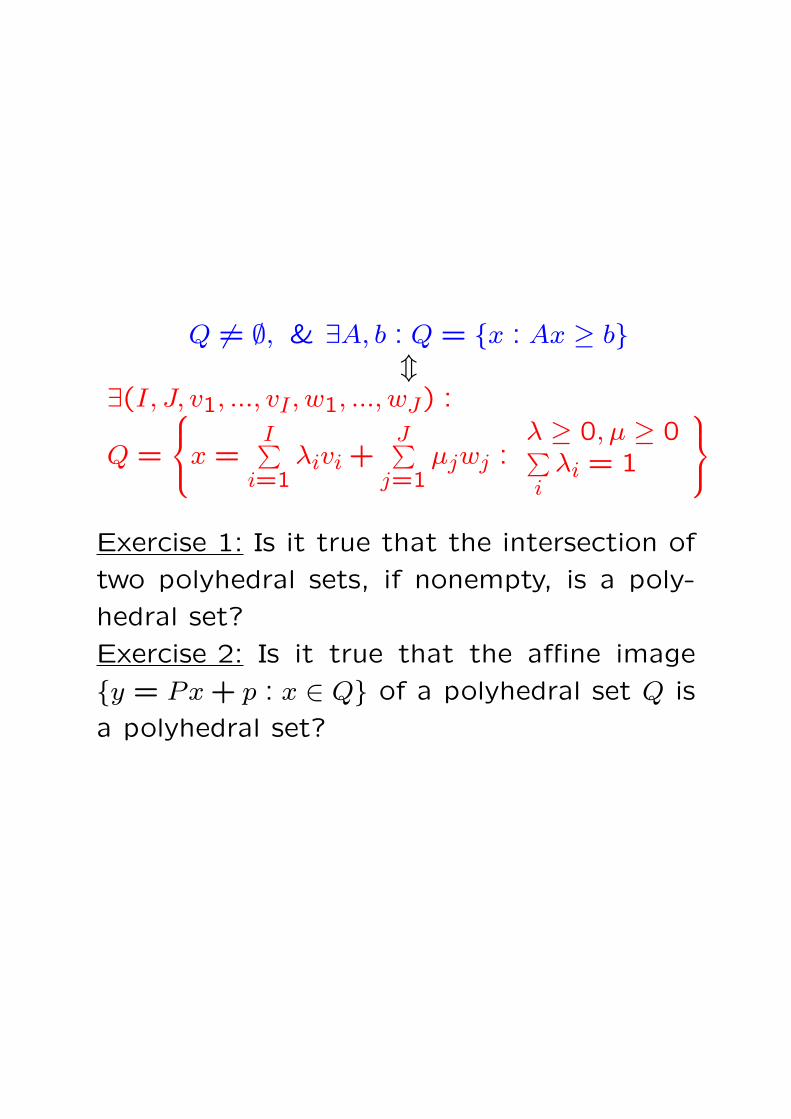
Q 6= ∅, & ∃A, b : Q = x : Ax ≥ bm
∃(I, J, v1, ..., vI , w1, ..., wJ) :
Q =
x =
I∑i=1
λivi +J∑
j=1µjwj :
λ ≥ 0, µ ≥ 0∑i
λi = 1
Exercise 1: Is it true that the intersection of
two polyhedral sets, if nonempty, is a poly-
hedral set?
Exercise 2: Is it true that the affine image
y = Px + p : x ∈ Q of a polyhedral set Q is
a polyhedral set?
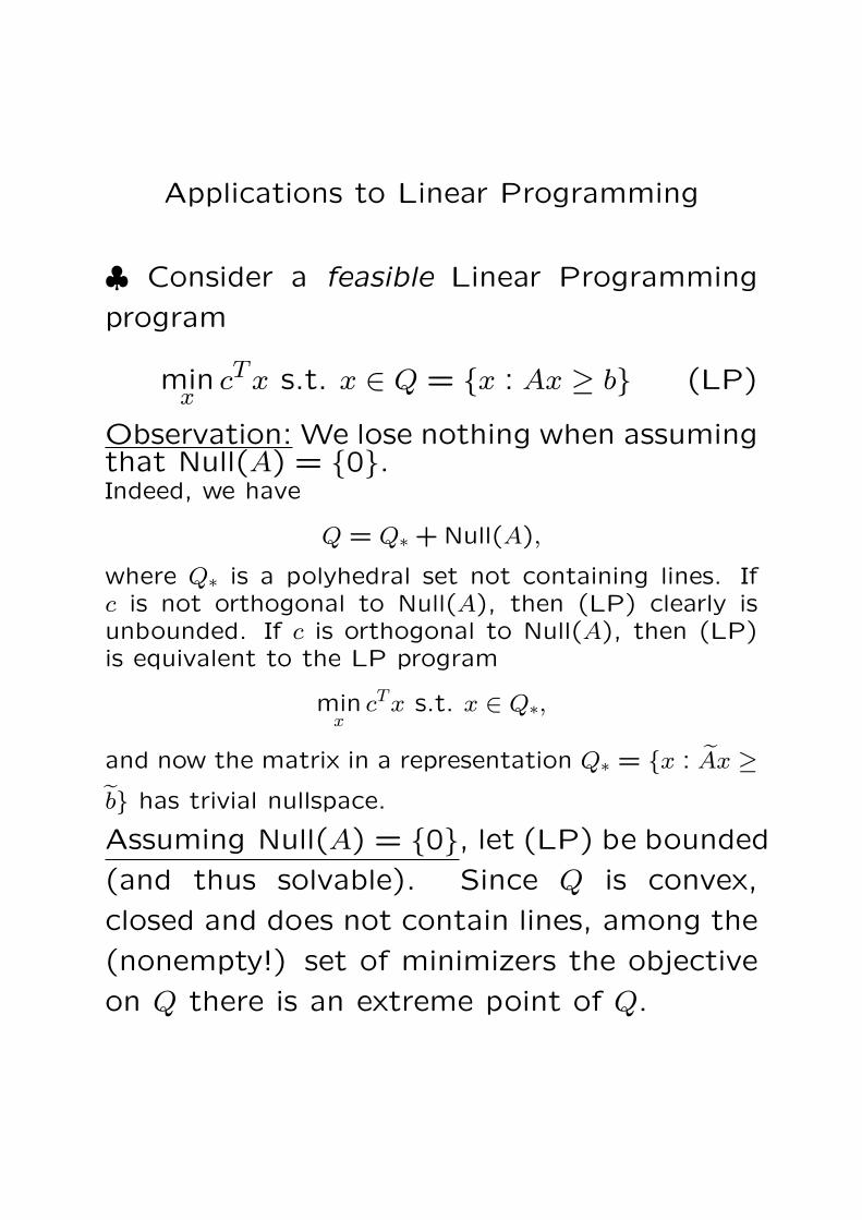
Applications to Linear Programming
♣ Consider a feasible Linear Programming
program
minx
cTx s.t. x ∈ Q = x : Ax ≥ b (LP)
Observation: We lose nothing when assumingthat Null(A) = 0.Indeed, we have
Q = Q∗ + Null(A),
where Q∗ is a polyhedral set not containing lines. Ifc is not orthogonal to Null(A), then (LP) clearly isunbounded. If c is orthogonal to Null(A), then (LP)is equivalent to the LP program
minx
cTx s.t. x ∈ Q∗,
and now the matrix in a representation Q∗ = x : Ax ≥b has trivial nullspace.
Assuming Null(A) = 0, let (LP) be bounded
(and thus solvable). Since Q is convex,
closed and does not contain lines, among the
(nonempty!) set of minimizers the objective
on Q there is an extreme point of Q.
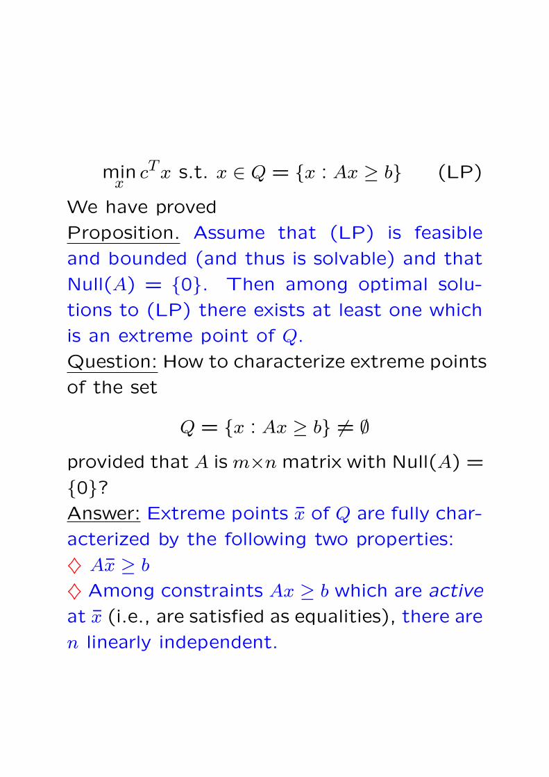
minx
cTx s.t. x ∈ Q = x : Ax ≥ b (LP)
We have proved
Proposition. Assume that (LP) is feasible
and bounded (and thus is solvable) and that
Null(A) = 0. Then among optimal solu-
tions to (LP) there exists at least one which
is an extreme point of Q.
Question: How to characterize extreme points
of the set
Q = x : Ax ≥ b 6= ∅provided that A is m×n matrix with Null(A) =
0?Answer: Extreme points x of Q are fully char-
acterized by the following two properties:
♦ Ax ≥ b
♦ Among constraints Ax ≥ b which are active
at x (i.e., are satisfied as equalities), there are
n linearly independent.
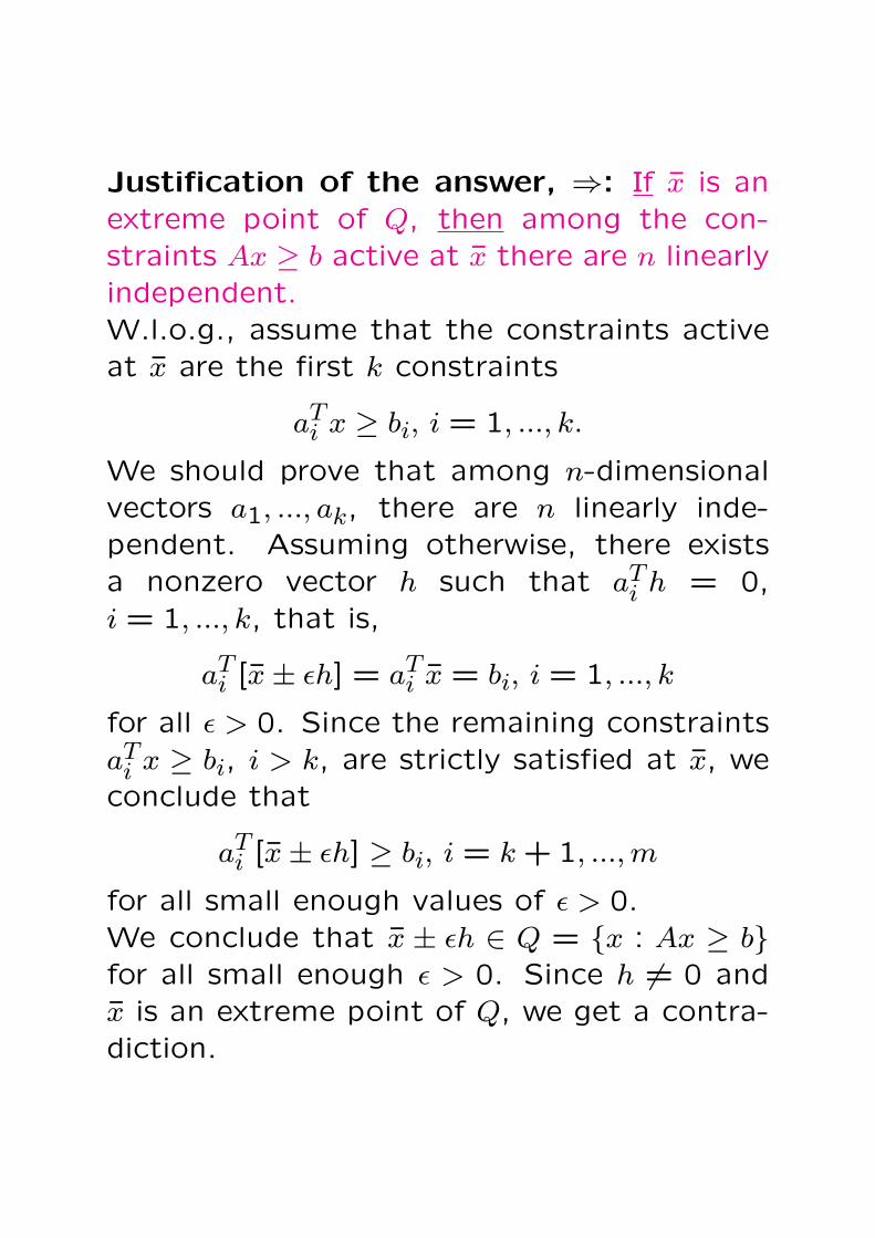
Justification of the answer, ⇒: If x is anextreme point of Q, then among the con-straints Ax ≥ b active at x there are n linearlyindependent.W.l.o.g., assume that the constraints activeat x are the first k constraints
aTi x ≥ bi, i = 1, ..., k.
We should prove that among n-dimensionalvectors a1, ..., ak, there are n linearly inde-pendent. Assuming otherwise, there existsa nonzero vector h such that aT
i h = 0,i = 1, ..., k, that is,
aTi [x± εh] = aT
i x = bi, i = 1, ..., k
for all ε > 0. Since the remaining constraintsaT
i x ≥ bi, i > k, are strictly satisfied at x, weconclude that
aTi [x± εh] ≥ bi, i = k + 1, ..., m
for all small enough values of ε > 0.We conclude that x ± εh ∈ Q = x : Ax ≥ bfor all small enough ε > 0. Since h 6= 0 andx is an extreme point of Q, we get a contra-diction.

Justification of the answer, ⇐: If x ∈ Q
makes equalities n of the constraints aTi x ≥ bi
with linearly independent vectors of coeffi-
cients, then x ∈ Ext(Q).
W.l.o.g., assume that n active at x con-
straints with linearly independent vectors of
coefficients are the first n constraints
aTi x ≥ bi, i = 1, ..., n.
We should prove that if h is such that x±h ∈Q, then h = 0. Indeed, we have
x± h ∈ Q ⇒ aTi [x± h] ≥ bi, i = 1, ..., n;
since aTi x = bi for i ≤ n, we get
aTi x± aT
i h = aTi [x± h] ≥ aT
i x, i = 1, ..., n,
whence
aTi h = 0, i = 1, ..., n. (∗)
Since n-dimensional vectors a1, ..., an are lin-
early independent, (∗) implies that h = 0,
Q.E.D.
Convex Functions
Definition: Let f be a real-valued function
defined on a nonempty subset Domf in Rn.
f is called convex, if
♦Domf is a convex set
♦for all x, y ∈ Domf and λ ∈ [0,1] one has
f(λx + (1− λ)y) ≤ λf(x) + (1− λ)f(y)
Equivalent definition: Let f be a real-valued
function defined on a nonempty subset Domf
in Rn. The function is called convex, if its
epigraph – the set
Epif = (x, t) ∈ Rn+1 : f(x) ≤ tis a convex set in Rn+1.
What does the definition of convexityactually mean?
The inequality
f(λx + (1− λ)y) ≤ λf(x) + (1− λ)f(y) (∗)where x, y ∈ Domf and λ ∈ [0,1] is automat-ically satisfied when x = y or when λ = 0/1.Thus, it says something only when the pointsx, y are distinct from each other and the pointz = λx+(1−λ)y is a (relative) interior pointof the segment [x, y]. What does (∗) say inthis case?♦Observe that z = λx + (1− λ)y = x + (1−λ)(y − x), whence
‖y − x‖ : ‖y − z‖ : ‖z − x‖ = 1 : λ : (1− λ)
Therefore
f(z) ≤ λf(x) + (1− λ)f(y) (∗)m
f(z)− f(x) ≤ (1− λ)︸ ︷︷ ︸‖z−x‖‖y−x‖
(f(y)− f(x))
mf(z)−f(x)‖z−x‖ ≤ f(y)−f(x)
‖y−x‖
Similarly,
f(z) ≤ λf(x) + (1− λ)f(y) (∗)m
λ︸︷︷︸‖y−z‖‖y−x‖
(f(y)− f(x)) ≤ f(y)− f(z)
mf(y)−f(x)‖y−x‖ ≤ f(y)−f(z)
‖y−z‖

Conclusion: f is convex iff for every three
distinct points x, y, z such that x, y ∈ Domf
and z ∈ [x, y], we have z ∈ Domf and
f(z)− f(x)
‖z − x‖ ≤ f(y)− f(x)
‖y − x‖ ≤ f(y)− f(z)
‖y − z‖ (∗)
Note: From 3 inequalities in (∗):f(z)−f(x)‖z−x‖ ≤ f(y)−f(x)
‖y−x‖f(y)−f(x)‖y−x‖ ≤ f(y)−f(z)
‖y−z‖f(z)−f(x)‖z−x‖ ≤ f(y)−f(z)
‖y−z‖every single one implies the other two.
x yz
Jensen’s Inequality: Let f(x) be a convex
function. Then
xi ∈ Domf, λi ≥ 0,∑i
λi = 1 ⇒f(
∑i
λixi) ≤∑i
λif(xi)
Proof: The points (xi, f(xi)) belong to Epif.Since this set is convex, the point
(∑
i
λixi,∑
i
λif(xi)) ∈ Epif.
By definition of the epigraph, it follows that
f(∑
i
λixi) ≤∑
i
λif(xi).
Extension: Let f be convex, Domf be closed
and f be continuous on Domf . Consider
a probability distribution π(dx) supported on
Domf . Then
f(Eπx) ≤ Eπf(x).
Examples:
♦Functions convex on R: • x2, x4, x6,...
• expxNonconvex functions on R: • x3 • sin(x)
♦Functions convex on R+: • xp, p ≥ 1
• −xp, 0 ≤ p ≤ 1 • x lnx
♦Functions convex on Rn: • affine function
f(x) = fT c
♦A norm ‖ · ‖ on Rn is a convex function:
‖λx + (1− λ)y‖ ≤ ‖λx‖+ ‖(1− λ)y‖[Triangle inequality]
= λ‖x‖+ (1− λ)‖y‖[homogeneity]
Application of Jensen’s Inequality: Let p =
pi > 0ni=1, q = qi > 0ni=1 be two discrete
probability distributions.
Claim: The Kullback-Liebler distance∑
i
pi lnpi
qi
between the distributions is ≥ 0.
Indeed, the function f(x) = − lnx, Domf =
x > 0, is convex. Setting xi = qi/pi, λi = pi
we have
0 = − ln
(∑i
qi
)= f(
∑i
pixi)
≤ ∑i
pif(xi) =∑i
pi(− ln qi/pi)
=∑i
pi ln(pi/qi)
What is the value of a convex function
outside its domain?
Convention. To save words, it is convenient
to think that a convex function f is defined
everywhere on Rn and takes real values and
value +∞. With this interpretation, f “re-
members” its domain:
Domf = x : f(x) ∈ Rx 6∈ Domf ⇒ f(x) = +∞
and the definition of convexity becomes
f(λx+(1−λ)y) ≤ λf(x)+(1−λ)f(y) ∀ x, y ∈ Rn
λ ∈ [0,1]
where the arithmetics of +∞ and reals is
given by the rules
a ∈ R⇒ a + (+∞) = (+∞) + (+∞) = +∞0 · (+∞) = +∞λ > 0 ⇒ λ · (+∞) = +∞Note: Operations like (+∞)−(+∞) or (−5) ·(+∞) are undefined!

♣ Convexity-preserving operations:
♦Taking conic combinations: If fi(x) are
convex function on Rn and λi ≥ 0, then the
function∑i
λifi(x) is convex
♦Affine substitution of argument: If f(x) is
convex function on Rn and x = Ay + b is an
affine mapping from Rk to Rn, then the func-
tion g(y) = f(Ax + b) is convex on Rm
♦Taking supremum: If fα(x), α ∈ A, is a
family of convex function on Rn, then the
function supα∈A
fα(x) is convex.
Proof: Episupα
fα(·) =⋂αEpifα(·), and in-
tersections of convex sets are convex.
♦Superposition Theorem: Let fi(x) be con-
vex functions on Rn, i = 1, ..., m, and F (y1, ..., ym)
be a convex and monotone function on Rm.
Then the function
g(x) =
F (f1(x), ..., fm(x)) , x ∈ Domfi, ∀i+∞ ,otherwise
is convex.
♦Partial minimization: Let f(x, y) be a con-vex function of z = (x, y) ∈ Rn, and let
g(x) = infy
f(x, y)
be > −∞ for all x. Then the function g(x) isconvex.Proof: g clearly takes real values and value+∞. Let us check the Convexity Inequality
g(λx′ + (1− λ)x′′) ≤ λg(x′) + (1− λ)g(x′′)[λ ∈ [0,1]]
There is nothing to check when λ = 0 orλ = 1, so let 0 < λ < 1. In this case, thereis nothing to check when g(x′) or g(x′′) is+∞, so let g(x′) < +∞, g(x′′) < +∞. Sinceg(x′) < +∞, for every ε > 0 there exists y′such that f(x′, y′) ≤ g(x′)+ε. Similarly, thereexists y′′ such that f(x′′, y′′) ≤ g(x′′)+ε. Now,
g(λx′ + (1− λ)x′′)≤ f(λx′ + (1− λ)x′′, λy′ + (1− λ)y′′)≤ λf(x′, y′) + (1− λ)f(x′′, y′′)≤ λ(g(x′) + ε) + (1− λ)(g(x′′) + ε)= λg(x′) + (1− λ)g(x′′) + ε
Since ε > 0 is arbitrary, we get
g(λx′ + (1− λ)x′′) ≤ λg(x′) + (1− λ)g(x′′).

How to detect convexity?
Convexity is one-dimensional property: A set
X ⊂ Rn is convex iff the set
t : a + th ∈ Xis, for every (a, h), a convex set on the axis
A function f on Rn is convex iff the function
φ(t) = f(a + th)
is, for every (a, h), a convex function on the
axis.

♣ When a function φ on the axis is convex?
Let φ be convex and finite on (a, b). This is
exactly the same as
φ(z)− φ(x)
z − x≤ φ(y)− φ(x)
y − x≤ φ(y)− φ(z)
y − z
when a < x < z < y < b. Assuming that
φ′(x) and φ′(y) exist and passing to limits as
z → x + 0 and z → y − 0, we get
φ′(x) ≤ φ(y)− φ(x)
y − x≤ φ′(y)
that is, φ′(x) is nondecreasing on the set of
points from (a, b) where it exists.

The following conditions are necessary and
sufficient for convexity of a univariate func-
tion:
♦The domain of the function φ should be an
open interval ∆ = (a, b), possibly with added
endpoint(s) (provided that the corresponding
endpoint(s) is/are finite)
♦φ should be continuous on (a, b) and dif-
ferentiable everywhere, except, perhaps, a
countable set, and the derivative should be
monotonically non-decreasing
♦at endpoint of (a, b) which belongs to
Domφ, φ is allowed to “jump up”, but not
to jump down.

♣ Sufficient condition for convexity of a uni-
variate function φ: Domφ is convex, φ is con-
tinuous on Domφ and is twice differentiable,
with nonnegative φ′′, on intDomφ.
Indeed, we should prove that under the con-
dition, if x < z < y are in Domφ, then
φ(z)− φ(x)
z − x≤ φ(y)− φ(z)
y − z
By Lagrange Theorem, the left ratio is φ′(ξ)for certain ξ ∈ (x, z), and the right ratio is
φ′(η) for certain η ∈ (z, y). Since φ′′(·) ≥ 0
and η > ξ, we have φ′(η) ≥ φ′(ξ), Q.E.D.

♣ Sufficient condition for convexity of a mul-
tivariate function f : Domf is convex, f is
continuous on Domf and is twice differen-
tiable, with positive semidefinite Hessian ma-
trix f ′′, on intDomf .
Instructive example: The function f(x) =
ln(n∑
i=1expxi) is convex on Rn.
Indeed,
hTf ′(x) =
∑i
expxihi∑i
expxi
hTf ′′(x)h = −
(∑i
expxihi
)2
(∑i
expxi)2 +
∑i
expxih2i∑
iexpxi

hTf ′′(x)h = −
∑iexpxihi
∑iexpxi
2
+
∑iexpxih2
i
∑iexpxi
Setting pi = expxi∑j
expxj, we have
hTf ′′(x)h =∑i
pih2i −
(∑i
pihi
)2
=∑i
pih2i −
(∑i
√pi(√
pihi)
)2
≥ ∑i
pih2i −
(∑i(√
pi)2
) (∑i(√
pihi)2
)
=∑i
pih2i −
(∑i
pih2i
)= 0
(note that∑i
pi = 1)
Corollary: When ci > 0, the function
g(y) = ln
∑
i
ci expaTi y
is convex.
Indeed,
g(y) = ln
∑
i
expln ci + aTi y
is obtained from the convex function
ln
∑
i
expxi
by affine substitution of argument.
Gradient Inequality
Proposition: Let f be a function, x be an
interior point of the domain of f and Q, x ∈Q, be a convex set such that f is convex on
Q. Assume that f is differentiable at x. Then
∀y ∈ Q : f(y) ≥ f(x) + (y − x)Tf ′(x). (∗)Proof. Let y ∈ Q. There is nothing to prove
when y = x or f(y) = +∞, thus, assume
that f(y) < ∞ and y 6= x. Let is set zε =
x + ε(y− x), 0 < ε < 1. Then zε is an interior
point of the segment [x, y]. Since f is convex,
we have
f(y)− f(x)
‖y − x‖ ≥ f(zε)− f(x)
‖zε − x‖ =f(x + ε(y − x))− f(x)
ε‖y − x‖Passing to limit as ε → +0, we arrive at
f(y)− f(x)
‖y − x‖ ≥ (y − x)Tf ′(x)‖y − x‖ ,
as required by (∗).

Lipschitz continuity of a convex function
Proposition: Let f be a convex function, andlet K be a closed and bounded set belongingto relative interior of the domain of f . Thenf is Lipschitz continuous on K, that is, thereexists a constant L < ∞ such that
|f(x)− f(y)| ≤ L‖x− y‖2 ∀x, y ∈ K.
Note: All three assumptions on K are essen-tial, as is shown by the following examples:♦f(x) = −√x, Domf = x ≥ 0, K = [0,1].Here K ⊂ Domf is closed and bounded, butis not contained in the relative interior ofDomf , and f is not Lipschitz continuous onK
♦f(x) = x2, Domf = K = R. Here K isclosed and belongs to rint Domf , but is un-bounded, and f is not Lipschitz continuouson K
♦f(x) = 1x, Domf = x > 0, K = (0,1].
Here K is bounded and belongs to rint Domf ,but is not closed, and f is not Lipschitz con-tinuous on K

Maxima and Minima of Convex Functions
(!) Proposition [“unimodality”] Let f be a
convex function and x∗ be a local minimizer
of f :
x∗ ∈ Domf&
∃r > 0 : f(x) ≥ f(x∗) ∀(x : ‖x− x∗‖ ≤ r).
Then x∗ is a global minimizer of f :
f(x) ≥ f(x∗) ∀x.
Proof: All we need to prove is that if x 6= x∗and x ∈ Domf , then f(x) ≥ f(x∗). To this
end let z ∈ (x∗, x). By convexity we have
f(z)− f(x∗)‖z − x∗‖
≤ f(x)− f(x∗)‖x− x∗‖
.
When z ∈ (x∗, x) is close enough to x∗, we
have f(z)−f(x∗)‖z−x∗‖ ≥ 0, whence f(x)−f(x∗)
‖x−x∗‖ ≥ 0,
that is, f(x) ≥ f(x∗).
Proposition Let f be a convex function. The
set of X∗ of global minimizers is convex.
Proof: This is an immediate corollary of im-
portant
Lemma: Let f be a convex function. Then
the level sets of f , that is, the sets
Xa = x : f(x) ≤ awhere a is a real, are convex.
Proof of Lemma: If x, y ∈ Xa and λ ∈ [0,1],
then
f(λx + (1− λ)y) ≤ λf(x) + (1− λ)f(y)≤ λa + (1− λ)a = a.
Thus, [x, y] ⊂ Xa.

♣ When the minimizer of a convex function
is unique?
Definition: A convex function is called strictly
convex, if
f(λx + (1− λ)y) < λf(x) + (1− λ)f(y)
whenever x 6= y and λ ∈ (0,1).
Note: If a convex function f has open do-
main and is twice continuously differentiable
on this domain with
hTf ′′(x)h > 0 ∀(x ∈ Domf, h 6= 0),
then f is strictly convex.
Proposition: For a strictly convex function f
a minimizer, if it exists, is unique.
Proof. Assume that X∗ = Argmin f contains
two distinct points x′, x′′. By strong convex-
ity,
f(1
2x′ + 1
2x′′) <
1
2
[f(x′) + f(x′′)
]= inf
xf,
which is impossible.
Theorem [Optimality conditions in convex
minimization] Let f be a function which is
differentiable at a point x∗ and is convex on
a convex set Q ⊂ Domf which contains x∗.A necessary and sufficient condition for f to
attain its minimum on Q at x∗ is
(x− x∗)Tf ′(x∗) ≥ 0 ∀x ∈ Q. (∗)Proof, ⇐: Assume that (∗) is valid, and let
us verify that f(x) ≥ f(x∗) for every x ∈ Q.
There is nothing to prove when x = x∗, thus,
let f(x) < ∞ and x 6= x∗. For zλ = x∗+λ(x−x∗) we have
f(zλ)− f(x∗)‖zλ − x∗‖
≤ f(x)− f(x∗)‖x− x∗‖
∀λ ∈ (0,1)
or, which is the same,
f(x∗ + λ[x− x∗])− f(x∗)λ‖x− x∗‖
≤ f(x)− f(x∗)‖x− x∗‖
∀λ ∈ (0,1)
As λ → +0, the left ratio converges to
(x−x∗)Tf ′(x∗)/‖x−x∗‖ ≥ 0; thus, f(x)−f(x∗)‖x−x∗‖ ≥
0, whence f(x) ≥ f(x∗).
“Let f be a function which is differen-
tiable at a point x∗ and is convex on
a convex set Q ⊂ Domf which con-
tains x∗. A necessary and sufficient
condition for f to attain its minimum
on Q at x∗ is
(x− x∗)Tf ′(x∗) ≥ 0 ∀x ∈ Q.′′
Proof, ⇒: Given that x∗ ∈ Argminy∈Q f(y),
let x ∈ Q. Then
0 ≤ f(x∗ + λ[x− x∗])− f(x∗)λ
∀λ ∈ (0,1),
whence (x− x∗)Tf ′(x∗) ≥ 0.
♣ Equivalent reformulation: Let f be a func-
tion which is differentiable at a point x∗ and
is convex on a convex set Q ⊂ Domf , x∗ ∈ Q.
Consider the radial cone of Q at x∗:
TQ(x∗) = h : ∃t > 0 : x∗ + th ∈ QNote: TQ(x∗) is indeed a cone which is com-
prised of all vectors of the form s(x − x∗),where x ∈ Q and s ≥ 0.
f attains its minimum on Q at x∗ iff
hTf ′(x∗) ≥ 0 ∀h ∈ TQ(x∗),
or, which is the same, iff
f ′(x∗) ∈ NQ(x∗) = g : gTh ≥ 0∀h ∈ TQ(x∗)︸ ︷︷ ︸normal cone of Q at x∗
.
(∗)
Example I: x∗ ∈ intQ. Here TQ(x∗) = Rn,
whence NQ(x∗) = 0, and (∗) becomes the
Fermat equation
f ′(x∗) = 0
Example II: x∗ ∈ rint Q. Let Aff(Q) = x∗+ L,
where L is a linear subspace in Rn. Here
TQ(x∗) = L, whence NQ(x∗) = L⊥. (∗) be-
comes the condition
f ′(x∗) is orthogonal to L.
Equivalently: Let Aff(Q) = x : Ax = b.Then L = x : Ax = 0, L⊥ = y = ATλ,and the optimality condition becomes
∃λ∗ :
∇∣∣∣x=x∗
[f(x) + (λ∗)T (Ax− b)] = 0
mf ′(x∗) +
∑i
λ∗i∇(aTi x− bi) = 0
[A =
aT1...
aTm
]
Example III: Q = x : Ax− b ≤ 0 is polyhedral.
In this case,
TQ(x∗)=
h : aT
i h ≤ 0 ∀i ∈ I(x∗) = i : aTi x∗ − bi = 0
.
By Homogeneous Farkas Lemma,
NQ(x∗) ≡ y : aTi h ≤ 0, i ∈ I(x∗) ⇒ yTh ≥ 0
= y = − ∑i∈I(x∗)
λiai : λi ≥ 0
and the optimality condition becomes
∃(λ∗i ≥ 0, i ∈ I(x∗)) : f ′(x∗) +∑
i∈I(x∗)λ∗i ai = 0
or, which is the same:
∃λ∗ ≥ 0 :
f ′(x∗) +m∑
i=1λ∗i ai = 0
λ∗i (aTi x∗ − bi) = 0, i = 1, ..., m
The point is that in the convex case these
conditions are necessary and sufficient for x∗to be a minimizer of f on Q.
Example: Let us solve the problem
minx
cTx +
m∑
i=1
xi lnxi : x ≥ 0,∑
i
xi = 1
.
The objective is convex, the domain Q =
x ≥ 0,∑i
xi = 1 is convex (and even poly-
hedral). Assuming that the minimum is
achieved at a point x∗ ∈ rint Q, the optimality
condition becomes
∇[cTx +
∑i
xi lnxi + λ[∑i
xi − 1]
]= 0
mlnxi = −ci − λ− 1 ∀i
mxi = exp1− λ exp−ci
Since∑i
xi should be 1, we arrive at
xi =exp−ci∑
jexp−cj
.
At this point, the optimality condition is sat-
isfied, so that the point indeed is a minimizer.
Maxima of convex functions
Proposition. Let f be a convex function.
Then
♦If f attains its maximum over Domf at a
point x∗ ∈ rint Domf , then f is constant on
Domf
♦If Domf is closed and does not contain lines
and f attains its maximum on Domf , then
among the maximizers there is an extreme
point of Domf
♦If Domf is polyhedral and f is bounded
from above on Domf , then f attains its max-
imum on Domf .
Subgradients of convex functions
♣ Let f be a convex function and x ∈intDomf . If f differentiable at x, then, by
Gradient Inequality, there exists an affine
function, specifically,
h(x) = f(x) + (x− x)Tf ′(x),
such that
f(x) ≥ h(x)∀x & f(x) = h(x) (∗)Affine function with property (∗) may exist
also in the case when f is not differentiable
at x ∈ Domf . (∗) implies that
h(x) = f(x) + (x− x)Tg (∗∗)for certain g. Function (∗∗) indeed satisfies
(∗) if and only if g is such that
f(x) ≥ f(x) + (x− x)Tg ∀x (!)
Definition. Let f be a convex function and
x ∈ Domf . Every vector g satisfying
f(x) ≥ f(x) + (x− x)Tg ∀x (!)
is called a subgradient of f at x. The set
of all subgradients, if any, of f at x is called
subdifferential ∂f(x) of f at x.
Example I: By Gradient Inequality, if con-
vex function f is differentiable at x, then
∇f(x) ∈ ∂f(x). If, in addition, x ∈ intDomf ,
then ∇f(x) is the unique element of ∂f(x).
Example II: Let f(x) = |x| (x ∈ R). When
x 6= 0, f is differentiable at x, whence
∂f(x) = f ′(x). When x = 0, subgradients
g are given by
|x| ≥ 0 + gx = gx ∀x,
that is, ∂f(0) = [−1,1].
Note: In the case in question, f has direc-
tional derivative
Df(x)[h] = limt→+0
f(x + th)− f(x)
t
at every point x ∈ R along every direction
h ∈ R, and this derivative is nothing but
Df(x)[h] = maxg∈∂f(x)
gTh
Proposition: Let f be convex. Then
♦For every x ∈ Domf , the subdifferential
∂f(x) is closed convex set
♦If x ∈ rint Domf , then ∂f(x) is nonempty.
♦If x ∈ rint Domf , then, for every h ∈ Rn,
∃Df(x)[h] ≡ limt→+0
f(x + th)− f(x)
t= max
g∈∂f(x)gTh.
♦Assume that x ∈ Domf is represented as
limi→∞xi with xi ∈ Domf and that
f(x) ≤ lim infi→∞ f(xi)
If a sequence gi ∈ ∂f(xi) converges to certain
vector g, then g ∈ ∂f(x).
♦The multi-valued mapping x 7→ ∂f(x) is lo-
cally bounded at every point x ∈ intDomf ,
that is, whenever x ∈ intDomf , there exist
r > 0 and R < ∞ such that
‖x− x‖2 ≤ r, g ∈ ∂f(x) ⇒ ‖g‖2 ≤ R.
Selected proof: “If x ∈ rint Domf , then∂f(x) is nonempty.”W.l.o.g. let Domf be full-dimensional, sothat x ∈ intDomf . Consider the convex set
T = Epif = (x, t) : t ≥ f(x).Since f is convex, it is continuous on intDomf ,whence T has a nonempty interior. The point(x, f(x)) clearly does not belong to this inte-rior, whence S = (x, f(x)) can be separatedfrom T : there exists (α, β) 6= 0 such that
αT x + βf(x) ≤ αTx + βt ∀(x, t ≥ f(x)) (∗)Clearly β ≥ 0 (otherwise (∗) will be impossi-ble when x = x and t > f(x) is large).Claim: β > 0. Indeed, with β = 0, (*) implies
αT x ≤ αTx ∀x ∈ Domf (∗∗)Since (α, β) 6= 0 and β = 0, we have α 6= 0;but then (∗∗) contradicts x ∈ intDomf .♦Since β > 0, (∗) implies that if g = β−1α,then
gT x + f(x) ≤ gTx + f(x) ∀x ∈ Domf,
that is,
f(x) ≥ f(x) + (x− x)Tg ∀x.
Elementary Calculus of Subgradients
♦If gi ∈ ∂fi(x) and λi ≥ 0, then∑
i
λigi ∈ ∂(∑
i
λifi)(x)
♦If gα ∈ ∂fα(x), α ∈ A,
f(·) = supα∈A
fα(·)
and
f(x) = fα(x), α ∈ A∗(x) 6= ∅,then every convex combination of vectors gα,
α ∈ A∗(x), is a subgradient of f at x
♦If gi ∈ domfi(x), i = 1, ..., m, and F (y1, ..., ym)
is convex and monotone and 0 ≤ d ∈∂F (f1(x), ..., fm(x)), then the vector
∑
i
digi
is a subgradient of F (f1(·), ..., fm(·)) at x.
Convex Programming
Lagrange Duality
Saddle Points
♣ Mathematical Programming program is
f∗ = minx
f(x) :g(x) ≡ (g1(x), ..., gm(x))T ≤ 0h(x) = (h1(x), ..., hk(x))
T = 0x ∈ X
(P )
♦x is the design vector. Values of x are called
solutions to (P )
♦f(x) is the objective
♦g(x) ≡ (g1(x), ..., gm(x))T ≤ 0 – inequality con-
straints
♦h(x) = (h1(x), ..., hk(x))T = 0 – equality con-
straints
♦X ⊂ Rn – domain. We always assume that
the objective and the constraints are well-
defined on X.
f∗ = minx
f(x) :g(x) ≡ (g1(x), ..., gm(x))T ≤ 0h(x) = (h1(x), ..., hk(x))
T = 0x ∈ X
(P )
♣ Solution x is called feasible, if it satisfies all
the constraints. Problem which has feasible
solutions is called feasible.
♣ If the objective is (below) bounded on
the set of feasible solutions, (P ) is called
bounded.
♣ The optimal value f∗ is
f∗ =
infxf(x) : x is feasible , (P ) is feasible
+∞, otherwise
f∗ is a real for feasible and bounded problem,
is −∞ for feasible unbounded problem, and
is +∞ for infeasible problem.
♣ Optimal solution of (P ) is a feasible solu-
tion x∗ such that f(x∗) = f∗. Problem which
has optimal solutions is called solvable.
f∗ = minx
f(x) :g(x) ≡ (g1(x), ..., gm(x))T ≤ 0h(x) = (h1(x), ..., hk(x))
T = 0x ∈ X
(P )
♣ Problem (P ) is called convex, if
♦X is a convex subset of Rn
♦f(·), g1(·),...,gm(·) are convex real-valued
functions on X
♦There are no equality constraints
[we could allow linear equality constraints,
but this does not add generality]
Preparing tools for Lagrange Duality:
Convex Theorem on Alternative
♣ Question: How to certify insolvability of
the system
f(x) < cgj(x) ≤ 0, j = 1, ..., m
x ∈ X(I)
♣ Answer: Assume that there exist nonnegative
weights λj, j = 1, ..., m, such that the in-
equality
f(x) +m∑
j=1
λjgj(x) < c
has no solutions in X:
∃λj ≥ 0 : infx∈X
[f(x) +m∑
j=1
λjgj(x)] ≥ c.
Then (I) is insolvable.

♣ Convex Theorem on Alternative: Consider
a system of constraints on x
f(x) < cgj(x) ≤ 0, j = 1, ..., m
x ∈ X(I)
along with system of constraints on λ:
infx∈X
[f(x) +m∑
j=1λjgj(x)] ≥ c
λj ≥ 0, j = 1, ..., m(II)
♦[Trivial part] If (II) is solvable, then (I) is
insolvable
♦[Nontrivial part] If (I) is insolvable and sys-
tem (I) is convex:
— X is convex set
— f , g1, ..., gm are real-valued convex func-
tions on X
and the subsystem
gj(x) < 0, j = 1, ..., m,x ∈ X
is solvable [Slater condition], then (II) is
solvable.

f(x) < cgj(x) ≤ 0, j = 1, ..., m
x ∈ X(I)
Proof of Nontrivial part: Assume that (I)
has no solutions. Consider two sets in Rm+1:
T︷ ︸︸ ︷
u ∈ Rm+1 : ∃x ∈ X :
f(x) ≤ u0g1(x) ≤ u1
..........gm(x) ≤ um
u ∈ Rm+1 : u0 < c, u1 ≤ 0, ..., um ≤ 0
︸ ︷︷ ︸
S
Observations: ♦S, T are convex and nonempty
♦S, T do not intersect (otherwise (I) would
have a solution)
Conclusion: S and T can be separated:
∃(a0, ..., am) 6= 0 : infu∈T
aTu ≥ supu∈S
aTu

T︷ ︸︸ ︷
u ∈ Rm+1 : ∃x ∈ X :
f(x) ≤ u0g1(x) ≤ u1
..........gm(x) ≤ um
u ∈ Rm+1 : u0 < c, u1 ≤ 0, ..., um ≤ 0
︸ ︷︷ ︸
S
∃(a0, ..., am) 6= 0 :infx∈X
infu0 ≥ f(x)u1 ≥ g1(x)
...um ≥ gm(x)
[a0u0 + a1u1 + ... + amum]
≥ supu0 < cu1 ≤ 0
...um ≤ 0
[a0u0 + a1u1 + ... + amum]
Conclusion: a ≥ 0, whence
infx∈X
[a0f(x) + a1g1(x) + ... + amgm(x)] ≥ a0c.
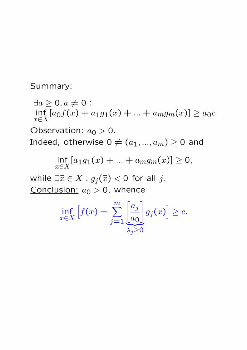
Summary:
∃a ≥ 0, a 6= 0 :infx∈X
[a0f(x) + a1g1(x) + ... + amgm(x)] ≥ a0c
Observation: a0 > 0.
Indeed, otherwise 0 6= (a1, ..., am) ≥ 0 and
infx∈X
[a1g1(x) + ... + amgm(x)] ≥ 0,
while ∃x ∈ X : gj(x) < 0 for all j.
Conclusion: a0 > 0, whence
infx∈X
[f(x) +
m∑
j=1
[aj
a0
]
︸ ︷︷ ︸λj≥0
gj(x)]≥ c.
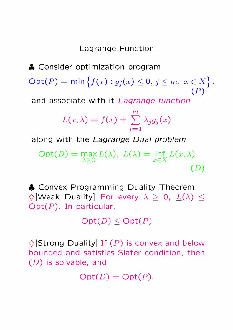
Lagrange Function
♣ Consider optimization program
Opt(P ) = minf(x) : gj(x) ≤ 0, j ≤ m, x ∈ X
.
(P )and associate with it Lagrange function
L(x, λ) = f(x) +m∑
j=1
λjgj(x)
along with the Lagrange Dual problem
Opt(D) = maxλ≥0
L(λ), L(λ) = infx∈X
L(x, λ)
(D)
♣ Convex Programming Duality Theorem:♦[Weak Duality] For every λ ≥ 0, L(λ) ≤Opt(P ). In particular,
Opt(D) ≤ Opt(P )
♦[Strong Duality] If (P ) is convex and belowbounded and satisfies Slater condition, then(D) is solvable, and
Opt(D) = Opt(P ).

Opt(P ) = min f(x) : gj(x) ≤ 0, j ≤ m, x ∈ X (P )⇓
L(x, λ) = f(x) +∑j
λjgj(x)
⇓Opt(D) = max
λ≥0
[infx∈X
L(x, λ)
]
︸ ︷︷ ︸L(λ)
(D)
Weak Duality: “Opt(D) ≤ Opt(P )”: There
is nothing to prove when (P ) is infeasible,
that is, when Opt(P ) = ∞. If x is feasible for
(P ) and λ ≥ 0, then L(x, λ) ≤ f(x), whence
λ ≥ 0 ⇒ L(λ) ≡ infx∈X
L(x, λ)
≤ infx∈X is feasible
L(x, λ)
≤ infx∈X is feasible
f(x)
= Opt(P )⇒ Opt(D) = sup
λ≥0L(λ) ≤ Opt(D).

Opt(P ) = min f(x) : gj(x) ≤ 0, j ≤ m, x ∈ X (P )⇓
L(x, λ) = f(x) +∑j
λjgj(x)
⇓Opt(D) = max
λ≥0
[infx∈X
L(x, λ)
]
︸ ︷︷ ︸L(λ)
(D)
Strong Duality: “If (P ) is convex and belowbounded and satisfies Slater condition, then(D) is solvable and Opt(D) = Opt(P )”:The system
f(x) < Opt(P ), gj(x) ≤ 0, j = 1, ..., m, x ∈ X
has no solutions, while the system
gj(x) < 0, j = 1, ..., m, x ∈ X
has a solution. By CTA,
∃λ∗ ≥ 0 : f(x) +∑
j
λ∗jgj(x) ≥ Opt(P ) ∀x ∈ X,
whence
L(λ∗) ≥ Opt(P ). (∗)Combined with Weak Duality, (∗) says that
Opt(D) = L(λ∗) = Opt(P ).

Opt(P ) = min f(x) : gj(x) ≤ 0, j ≤ m, x ∈ X (P )⇓
L(x, λ) = f(x) +∑j
λjgj(x)
⇓Opt(D) = max
λ≥0
[infx∈X
L(x, λ)
]
︸ ︷︷ ︸L(λ)
(D)
Note: The Lagrange function “remembers”,
up to equivalence, both (P ) and (D).
Indeed,
Opt(D) = supλ≥0
infx∈X
L(x, λ)
is given by the Lagrange function. Now con-
sider the function
L(x) = supλ≥0
L(x, λ) =
f(x), gj(x) ≤ 0, j ≤ m+∞, otherwise
(P ) clearly is equivalent to the problem of
minimizing L(x) over x ∈ X:
Opt(P ) = infx∈X
supλ≥0
L(x, λ)

Saddle Points
♣ Let X ⊂ Rn, Λ ⊂ Rm be nonempty sets, and
let F (x, λ) be a real-valued function on X×Λ.
This function gives rise to two optimization
problems
Opt(P ) = infx∈X
F (x)︷ ︸︸ ︷supλ∈Λ
F (x, λ) (P )
Opt(D) = supλ∈Λ
infx∈X
F (x, λ)︸ ︷︷ ︸
F (λ)
(D)

Opt(P ) = infx∈X
F (x)︷ ︸︸ ︷supλ∈Λ
F (x, λ) (P )
Opt(D) = supλ∈Λ
infx∈X
F (x, λ)︸ ︷︷ ︸
F (λ)
(D)
Game interpretation: Player I chooses x ∈ X,player II chooses λ ∈ Λ. With choices of theplayers x, λ, player I pays to player II the sumof F (x, λ). What should the players do tooptimize their wealth?♦If Player I chooses x first, and Player IIknows this choice when choosing λ, II willmaximize his profit, and the loss of I will beF (x). To minimize his loss, I should solve(P ), thus ensuring himself loss Opt(P ) orless.♦If Player II chooses λ first, and Player Iknows this choice when choosing x, I willminimize his loss, and the profit of II will beF (λ). To maximize his profit, II should solve(D), thus ensuring himself profit Opt(D) ormore.
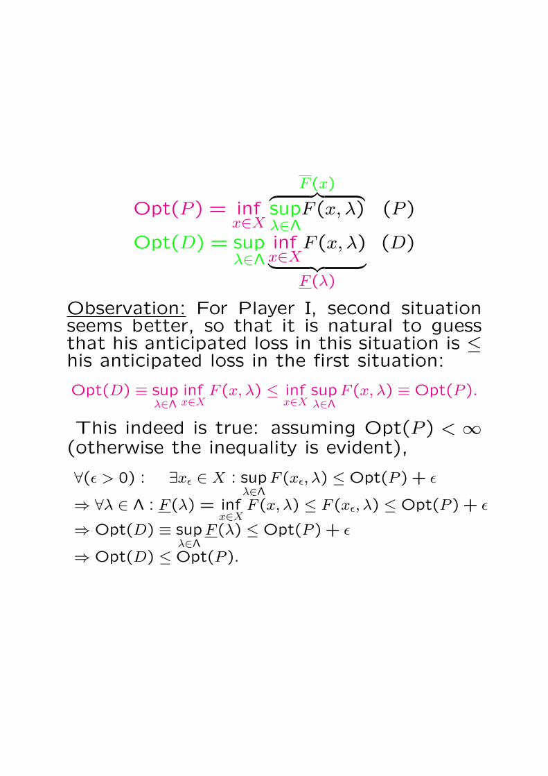
Opt(P ) = infx∈X
F (x)︷ ︸︸ ︷supλ∈Λ
F (x, λ) (P )
Opt(D) = supλ∈Λ
infx∈X
F (x, λ)︸ ︷︷ ︸
F (λ)
(D)
Observation: For Player I, second situationseems better, so that it is natural to guessthat his anticipated loss in this situation is ≤his anticipated loss in the first situation:
Opt(D) ≡ supλ∈Λ
infx∈X
F (x, λ) ≤ infx∈X
supλ∈Λ
F (x, λ) ≡ Opt(P ).
This indeed is true: assuming Opt(P ) < ∞(otherwise the inequality is evident),
∀(ε > 0) : ∃xε ∈ X : supλ∈Λ
F (xε, λ) ≤ Opt(P ) + ε
⇒ ∀λ ∈ Λ : F (λ) = infx∈X
F (x, λ) ≤ F (xε, λ) ≤ Opt(P ) + ε
⇒ Opt(D) ≡ supλ∈Λ
F (λ) ≤ Opt(P ) + ε
⇒ Opt(D) ≤ Opt(P ).

Opt(P ) = infx∈X
F (x)︷ ︸︸ ︷supλ∈Λ
F (x, λ) (P )
Opt(D) = supλ∈Λ
infx∈X
F (x, λ)︸ ︷︷ ︸
F (λ)
(D)
♣ What should the players do when making
their choices simultaneously?
A “good case” when we can answer this
question – F has a saddle point.
Definition: We call a point (x∗, λ∗) ∈ X ×Λ a
saddle point of F , if
F (x, λ∗) ≥ F (x∗, λ∗) ≥ F (x∗, λ) ∀(x ∈ X, λ ∈ Λ).
In game terms, a saddle point is an equi-
librium – no one of the players can improve
his wealth, provided the adversary keeps his
choice unchanged.
Proposition: F has a saddle point if and only
if both (P ) and (D) are solvable with equal
optimal values. In this case, the saddle points
of F are exactly the pairs (x∗, λ∗), where x∗is an optimal solution to (P ), and λ∗ is an
optimal solution to (D).

Opt(P ) = infx∈X
F (x)︷ ︸︸ ︷supλ∈Λ
F (x, λ) (P )
Opt(D) = supλ∈Λ
infx∈X
F (x, λ)︸ ︷︷ ︸
F (λ)
(D)
Proof, ⇒: Assume that (x∗, λ∗) is a saddle
point of F , and let us prove that x∗ solves
(P ), λ∗ solves (D), and Opt(P ) = Opt(D).
Indeed, we have
F (x, λ∗) ≥ F (x∗, λ∗) ≥ F (x∗, λ) ∀(x ∈ X, λ ∈ Λ)
whence
Opt(P ) ≤ F (x∗) = supλ∈Λ
F (x∗, λ) = F (x∗, λ∗)
Opt(D) ≥ F (λ∗) = infx∈X
F (x, λ∗) = F (x∗, λ∗)
Since Opt(P ) ≥ Opt(D), we see that all in-
equalities in the chain
Opt(P ) ≤ F (x∗) = F (x∗, λ∗) = F (λ∗) ≤ Opt(D)
are equalities. Thus, x∗ solves (P ), λ∗ solves
(D) and Opt(P ) = Opt(D).

Opt(P ) = infx∈X
F (x)︷ ︸︸ ︷supλ∈Λ
F (x, λ) (P )
Opt(D) = supλ∈Λ
infx∈X
F (x, λ)︸ ︷︷ ︸
F (λ)
(D)
Proof, ⇐. Assume that (P ), (D) have op-
timal solutions x∗, λ∗ and Opt(P ) = Opt(D),
and let us prove that (x∗, λ∗) is a saddle point.
We have
Opt(P ) = F (x∗) = supλ∈Λ
F (x∗, λ) ≥ F (x∗, λ∗)
Opt(D) = F (λ∗) = infx∈X
F (x, λ∗) ≤ F (x∗, λ∗)(∗)
Since Opt(P ) = Opt(D), all inequalities in
(∗) are equalities, so that
supλ∈Λ
F (x∗, λ) = F (x∗λ∗) = infx∈X
F (x, λ∗).
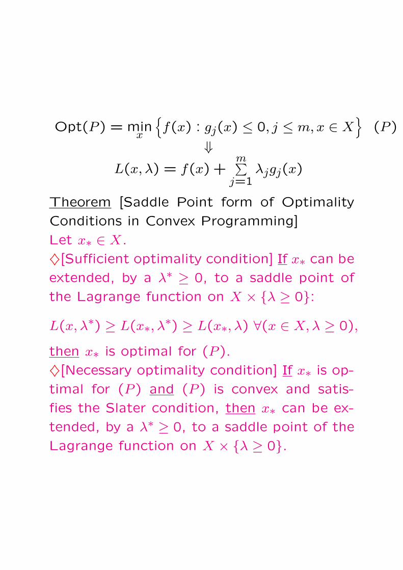
Opt(P ) = minx
f(x) : gj(x) ≤ 0, j ≤ m, x ∈ X
(P )
⇓L(x, λ) = f(x) +
m∑j=1
λjgj(x)
Theorem [Saddle Point form of Optimality
Conditions in Convex Programming]
Let x∗ ∈ X.
♦[Sufficient optimality condition] If x∗ can be
extended, by a λ∗ ≥ 0, to a saddle point of
the Lagrange function on X × λ ≥ 0:
L(x, λ∗) ≥ L(x∗, λ∗) ≥ L(x∗, λ) ∀(x ∈ X, λ ≥ 0),
then x∗ is optimal for (P ).
♦[Necessary optimality condition] If x∗ is op-
timal for (P ) and (P ) is convex and satis-
fies the Slater condition, then x∗ can be ex-
tended, by a λ∗ ≥ 0, to a saddle point of the
Lagrange function on X × λ ≥ 0.
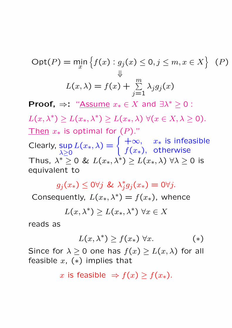
Opt(P ) = minx
f(x) : gj(x) ≤ 0, j ≤ m, x ∈ X
(P )
⇓L(x, λ) = f(x) +
m∑j=1
λjgj(x)
Proof, ⇒: “Assume x∗ ∈ X and ∃λ∗ ≥ 0 :
L(x, λ∗) ≥ L(x∗, λ∗) ≥ L(x∗, λ) ∀(x ∈ X, λ ≥ 0).
Then x∗ is optimal for (P ).”
Clearly, supλ≥0
L(x∗, λ) =
+∞, x∗ is infeasiblef(x∗), otherwise
Thus, λ∗ ≥ 0 & L(x∗, λ∗) ≥ L(x∗, λ) ∀λ ≥ 0 isequivalent to
gj(x∗) ≤ 0∀j & λ∗jgj(x∗) = 0∀j.Consequently, L(x∗, λ∗) = f(x∗), whence
L(x, λ∗) ≥ L(x∗, λ∗) ∀x ∈ X
reads as
L(x, λ∗) ≥ f(x∗) ∀x. (∗)Since for λ ≥ 0 one has f(x) ≥ L(x, λ) for allfeasible x, (∗) implies that
x is feasible ⇒ f(x) ≥ f(x∗).
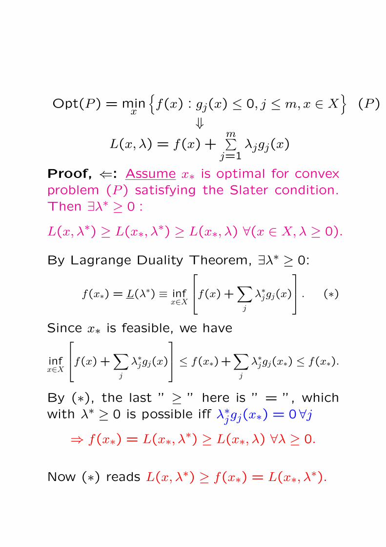
Opt(P ) = minx
f(x) : gj(x) ≤ 0, j ≤ m, x ∈ X
(P )
⇓L(x, λ) = f(x) +
m∑j=1
λjgj(x)
Proof, ⇐: Assume x∗ is optimal for convexproblem (P ) satisfying the Slater condition.Then ∃λ∗ ≥ 0 :
L(x, λ∗) ≥ L(x∗, λ∗) ≥ L(x∗, λ) ∀(x ∈ X, λ ≥ 0).
By Lagrange Duality Theorem, ∃λ∗ ≥ 0:
f(x∗) = L(λ∗) ≡ infx∈X
f(x) +
∑
j
λ∗jgj(x)
. (∗)
Since x∗ is feasible, we have
infx∈X
f(x) +
∑
j
λ∗jgj(x)
≤ f(x∗)+
∑
j
λ∗jgj(x∗) ≤ f(x∗).
By (∗), the last ” ≥ ” here is ” = ”, whichwith λ∗ ≥ 0 is possible iff λ∗jgj(x∗) = 0∀j
⇒ f(x∗) = L(x∗, λ∗) ≥ L(x∗, λ) ∀λ ≥ 0.
Now (∗) reads L(x, λ∗) ≥ f(x∗) = L(x∗, λ∗).

Opt(P ) = minx
f(x) : gj(x) ≤ 0, j ≤ m, x ∈ X
(P )
⇓L(x, λ) = f(x) +
m∑j=1
λjgj(x)
Theorem [Karush-Kuhn-Tucker Optimality Con-
ditions in Convex Programming] Let (P ) be
a convex program, let x∗ be its feasible so-
lution, and let the functions f , g1,...,gm be
differentiable at x∗. Then
♦The Karush-Kuhn-Tucker condition:
Exist Lagrange multipliers λ∗ ≥ 0 such that
∇f(x∗) +m∑
j=1λ∗j∇gj(x∗) ∈ N∗
X(x∗)
λ∗jgj(x∗) = 0, j ≤ m [complementary slackness]
is sufficient for x∗ to be optimal.
♦If (P ) satisfies restricted Slater condition:
∃x ∈ rint X : gj(x) ≤ 0 for all constraints and
gj(x) < 0 for all nonlinear constraints,
then the KKT is necessary and sufficient for
x∗ to be optimal.

Opt(P ) = minx
f(x) : gj(x) ≤ 0, j ≤ m, x ∈ X
(P )
⇓L(x, λ) = f(x) +
m∑j=1
λjgj(x)
Proof, ⇒: Let (P ) be convex, x∗ be feasible,and f , gj be differentiable at x∗. Assume alsothat the KKT holds:Exist Lagrange multipliers λ∗ ≥ 0 such that
(a) ∇f(x∗) +m∑
j=1λ∗j∇gj(x∗) ∈ N∗
X(x∗)
(b) λ∗jgj(x∗) = 0, j ≤ m [complementary slackness]
Then x∗ is optimal.Indeed, complementary slackness plus λ∗ ≥ 0ensure that
L(x∗, λ∗) ≥ L(x∗, λ) ∀λ ≥ 0.
Further, L(x, λ∗) is convex in x ∈ X and dif-ferentiable at x∗ ∈ X, so that (a) implies that
L(x, λ∗) ≥ L(x∗, λ∗) ∀x ∈ X.
Thus, x∗ can be extended to a saddle pointof the Lagrange function and therefore is op-timal for (P ).

Opt(P ) = minx
f(x) : gj(x) ≤ 0, j ≤ m, x ∈ X
(P )
⇓L(x, λ) = f(x) +
m∑j=1
λjgj(x)
Proof, ⇐ [under Slater condition] Let (P )be convex and satisfy the Slater condition, letx∗ be optimal and f , gj be differentiable atx∗. ThenExist Lagrange multipliers λ∗ ≥ 0 such that
(a) ∇f(x∗) +m∑
j=1λ∗j∇gj(x∗) ∈ N∗
X(x∗)
(b) λ∗jgj(x∗) = 0, j ≤ m [complementary slackness]
By Saddle Point Optimality condition, fromoptimality of x∗ it follows that ∃λ∗ ≥ 0 suchthat (x∗, λ∗) is a saddle point of L(x, λ) onX × λ ≥ 0. This is equivalent to
λ∗jgj(x∗) = 0 ∀j & minx∈X
L(x, λ∗) = L(x∗, λ∗)︸ ︷︷ ︸
(∗)Since the function L(x, λ∗) is convex in x ∈X and differentiable at x∗ ∈ X, relation (∗)implies (a).
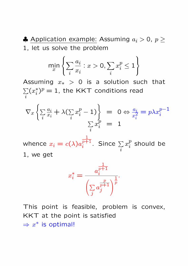
♣ Application example: Assuming ai > 0, p ≥1, let us solve the problem
minx
∑
i
ai
xi: x > 0,
∑
i
xpi ≤ 1
Assuming x∗ > 0 is a solution such that∑i(x∗i )p = 1, the KKT conditions read
∇x
∑i
aixi
+ λ(∑i
xpi − 1)
= 0 ⇔ ai
x2i= pλx
p−1i
∑i
xpi = 1
whence xi = c(λ)a1
p+1i . Since
∑i
xpi should be
1, we get
x∗i =a
1p+1i
(∑j
ap
p+1j
)1p
.
This point is feasible, problem is convex,
KKT at the point is satisfied
⇒ x∗ is optimal!

Existence of Saddle Points
♣ Theorem [Sion-Kakutani] Let X ⊂ Rn,Λ ⊂ Rm be nonempty convex closed sets andF (x, λ) : X × Λ → R be a continuous func-tion which is convex in x ∈ X and concave inλ ∈ Λ.Assume that X is compact, and that thereexists x ∈ X such that all the sets
Λa : λ ∈ Λ : F (x, λ) ≥ aare bounded (e.g., Λ is bounded).Then F possesses a saddle point on X → Λ.Proof:MiniMax Lemma: Let fi(x), i = 1, ..., m, beconvex continuous functions on a convexcompact set X ⊂ Rn. Then there existsµ∗ ≥ 0 with
∑i
µ∗i = 1 such that
minx∈X
max1≤i≤m
fi(x) = minx∈X
∑
i
µ∗i fi(x)
Note: When µ ≥ 0,∑i
µi = 1, one has
max1≤i≤m
fi(x) ≥∑i
µifi(x)
⇒ minx∈X
maxi
fi(x) ≥ minx∈X
∑i
µifi(x)
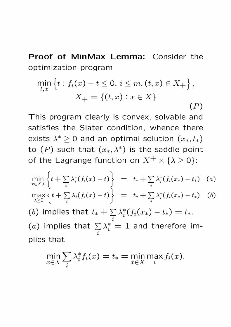
Proof of MinMax Lemma: Consider the
optimization program
mint,x
t : fi(x)− t ≤ 0, i ≤ m, (t, x) ∈ X+
,
X+ = (t, x) : x ∈ X(P )
This program clearly is convex, solvable and
satisfies the Slater condition, whence there
exists λ∗ ≥ 0 and an optimal solution (x∗, t∗)to (P ) such that (x∗, λ∗) is the saddle point
of the Lagrange function on X+ × λ ≥ 0:
minx∈X,t
t +
∑i
λ∗i (fi(x)− t)
= t∗ +
∑i
λ∗i (fi(x∗)− t∗) (a)
maxλ≥0
t +
∑i
λi(fi(x)− t)
= t∗ +
∑i
λ∗i (fi(x∗)− t∗) (b)
(b) implies that t∗ +∑i
λ∗i (fi(x∗)− t∗) = t∗.
(a) implies that∑i
λ∗i = 1 and therefore im-
plies that
minx∈X
∑
i
λ∗i fi(x) = t∗ = minx∈X
maxi
fi(x).

Proof of Sion-Kakutani Theorem: We
should prove that problems
Opt(P ) = infx∈X
F (x)︷ ︸︸ ︷supλ∈Λ
F (x, λ) (P )
Opt(D) = supλ∈Λ
infx∈X
F (x, λ)︸ ︷︷ ︸
F (λ)
(D)
are solvable with equal optimal values.
10. Since X is compact and F (x, λ) is con-
tinuous on X × λ, the function F (λ) is con-
tinuous on Λ. Besides this, the sets
Λa = λ ∈ Λ : F (λ) ≥ aare contained in the sets
Λa = λ ∈ Λ : F (x, λ) ≥ aand therefore are bounded. Finally, Λ is
closed, so that the continuous function F (·)with bounded level sets Λa attains it maxi-
mum on a closed set Λ. Thus, (D) is solv-
able; let λ∗ be an optimal solution to (D).
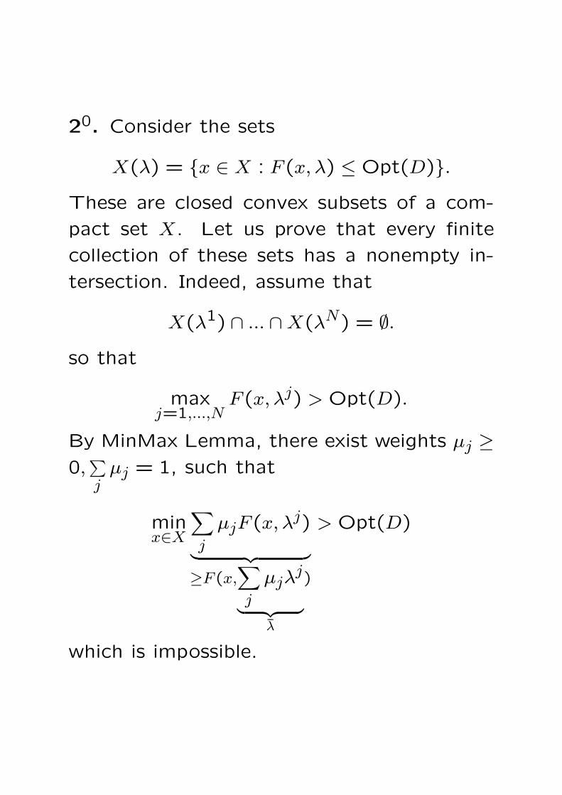
20. Consider the sets
X(λ) = x ∈ X : F (x, λ) ≤ Opt(D).These are closed convex subsets of a com-
pact set X. Let us prove that every finite
collection of these sets has a nonempty in-
tersection. Indeed, assume that
X(λ1) ∩ ... ∩X(λN) = ∅.so that
maxj=1,...,N
F (x, λj) > Opt(D).
By MinMax Lemma, there exist weights µj ≥0,
∑j
µj = 1, such that
minx∈X
∑
j
µjF (x, λj)
︸ ︷︷ ︸≥F (x,
∑
j
µjλj
︸ ︷︷ ︸λ
)
> Opt(D)
which is impossible.
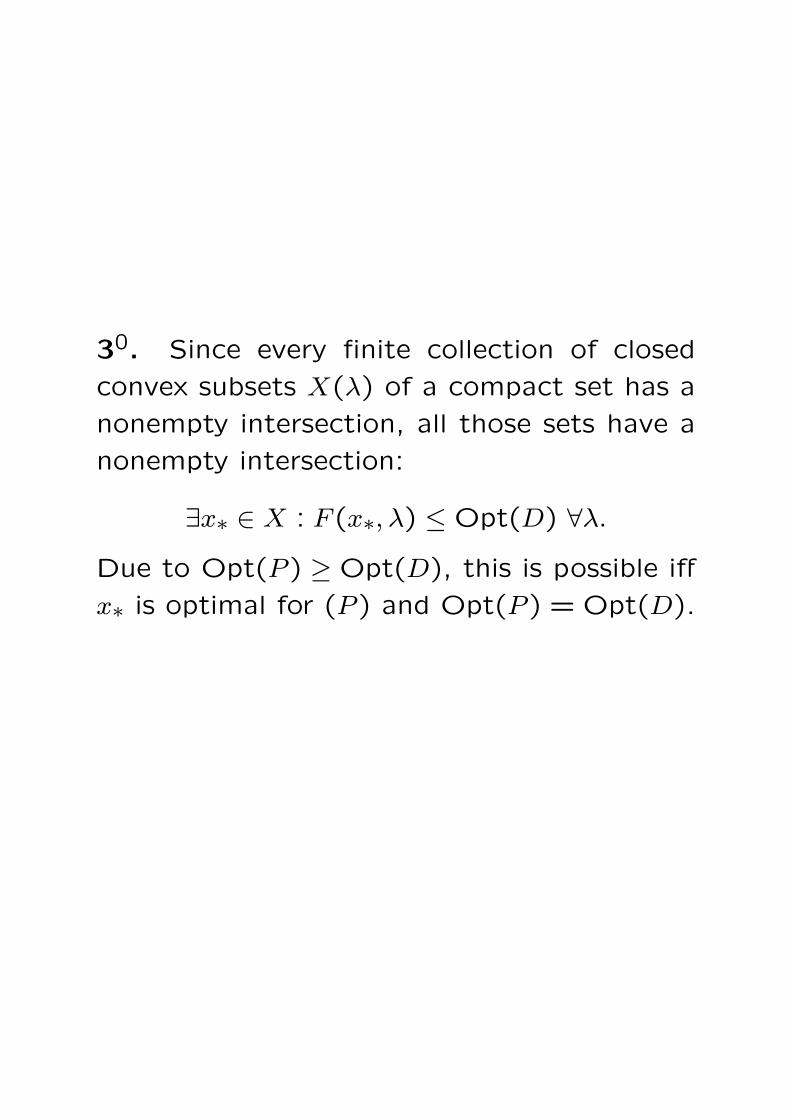
30. Since every finite collection of closed
convex subsets X(λ) of a compact set has a
nonempty intersection, all those sets have a
nonempty intersection:
∃x∗ ∈ X : F (x∗, λ) ≤ Opt(D) ∀λ.
Due to Opt(P ) ≥ Opt(D), this is possible iff
x∗ is optimal for (P ) and Opt(P ) = Opt(D).

Optimality Conditions in MathematicalProgramming
♣ Situation: We are given a MathematicalProgramming problem
minx
f(x) :(g1(x), g2(x), ..., gm(x)) ≤ 0
(h1(x), ..., hk(x)) = 0x ∈ X
.
(P )
Question of interest: Assume that we aregiven a feasible solution x∗ to (P ). Whatare the conditions (necessary, sufficient, nec-essary and sufficient) for x∗ to be optimal?Fact: Except for convex programs, there areno verifiable local sufficient conditions forglobal optimality. There exist, however,♦verifiable local necessary conditions for lo-cal (and thus – for global) optimality♦verifiable local sufficient conditions for lo-cal optimalityFact: Existing conditions for local optimalityassume that x∗ ∈ intX, which, from the view-point of local optimality of x∗, is exactly thesame as to say that X = Rn.

♣ Situation: We are given a Mathematical
Programming problem
minx
f(x) :
(g1(x), g2(x), ..., gm(x)) ≤ 0(h1(x), ..., hk(x)) = 0
.
(P )
and a feasible solution x∗ to the problem, and
are interested in necessary/sufficient condi-
tions for local optimality of x∗:There exists r > 0 such that for every feasible
x with ‖x− x∗‖ ≤ r one has
f(x) ≥ f(x∗).
Default assumption: The objective and all
the constraints are continuously differen-
tiable in a neighbourhood of x∗.

minx
f(x) :
(g1(x), g2(x), ..., gm(x)) ≤ 0(h1(x), ..., hk(x)) = 0
.
(P )
♣ First Order Optimality Conditions are ex-
pressed via values and gradients of the ob-
jective and the constraints at x∗. Except for
convex case, only necessary First Order con-
ditions are known.

minx
f(x) :
(g1(x), g2(x), ..., gm(x)) ≤ 0(h1(x), ..., hk(x)) = 0
.
(P )
The idea:
♦Assume that x∗ is locally optimal for (P ).
Let us approximate (P ) around x∗ by a Linear
Programming program
minx
f(x∗) + (x− x∗)Tf ′(x∗)s.t.
0︷ ︸︸ ︷gj(x∗)+(x− x∗)Tg′j(x∗) ≤ 0, j ∈ J(x∗)hi(x∗)︸ ︷︷ ︸
0
+(x− x∗)Th′i(x∗) = 0, 1 ≤ i ≤ k
[J(x∗) = j : gj(x∗) = 0
]
(LP )
Note: Since all gj(·) are continuous at x∗, the
non-active at x∗ inequality constraints (those
with gj(x∗) < 0) do not affect (LP ).
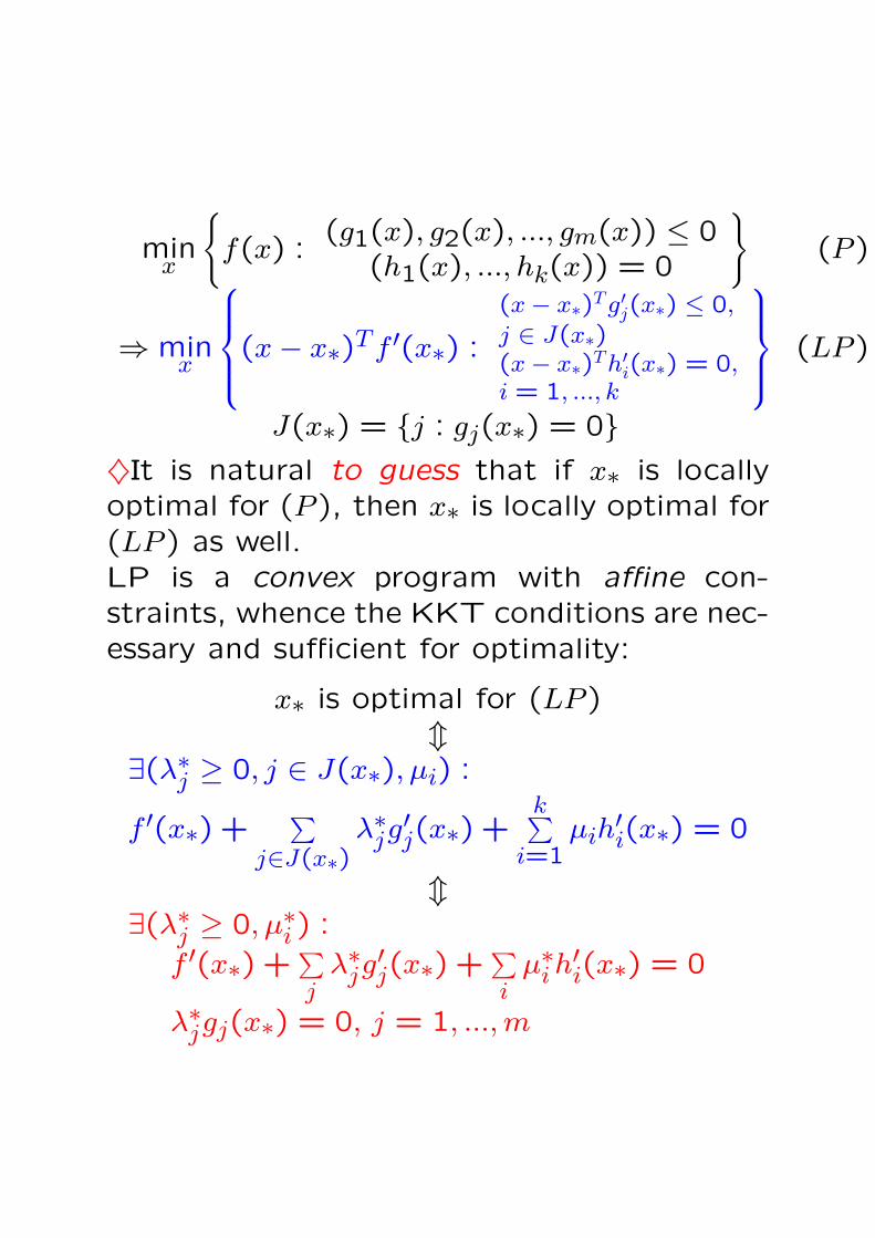
minx
f(x) :
(g1(x), g2(x), ..., gm(x)) ≤ 0(h1(x), ..., hk(x)) = 0
(P )
⇒ minx
(x− x∗)Tf ′(x∗) :
(x− x∗)Tg′j(x∗) ≤ 0,j ∈ J(x∗)(x− x∗)Th′i(x∗) = 0,i = 1, ..., k
(LP )
J(x∗) = j : gj(x∗) = 0♦It is natural to guess that if x∗ is locallyoptimal for (P ), then x∗ is locally optimal for(LP ) as well.LP is a convex program with affine con-straints, whence the KKT conditions are nec-essary and sufficient for optimality:
x∗ is optimal for (LP )m
∃(λ∗j ≥ 0, j ∈ J(x∗), µi) :
f ′(x∗) +∑
j∈J(x∗)λ∗jg′j(x∗) +
k∑i=1
µih′i(x∗) = 0
m∃(λ∗j ≥ 0, µ∗i ) :
f ′(x∗) +∑j
λ∗jg′j(x∗) +∑i
µ∗i h′i(x∗) = 0
λ∗jgj(x∗) = 0, j = 1, ..., m

minx
f(x) :
(g1(x), g2(x), ..., gm(x)) ≤ 0(h1(x), ..., hk(x)) = 0
(P )
Proposition. Let x∗ be a locally optimal so-
lution of (P ).
Assume that x∗ remains locally optimal when
passing from (P ) to the linearized problem
minx
(x− x∗)Tf ′(x∗) :
(x− x∗)Tg′j(x∗) ≤ 0,j ∈ J(x∗)(x− x∗)Th′i(x∗) = 0,i = 1, ..., k
(LP )
Then at x∗ the KKT condition holds:
∃(λ∗j ≥ 0, µ∗i ) :
f ′(x∗) +∑j
λ∗jg′j(x∗) +∑i
µ∗i h′i(x∗) = 0
λ∗jgj(x∗) = 0, j = 1, ..., m

minx
f(x) :
(g1(x), g2(x), ..., gm(x)) ≤ 0(h1(x), ..., hk(x)) = 0
(P )
minx
(x− x∗)Tf ′(x∗) :
(x− x∗)Tg′j(x∗) ≤ 0,j ∈ J(x∗)(x− x∗)Th′i(x∗) = 0,i = 1, ..., k
(LP )
To make Proposition useful, we need a ver-
ifiable sufficient condition for “x∗ remains
locally optimal when passing from (P ) to
(LP )”.
The most natural form of such a condition is
regularity:
Gradients, taken at x∗, of all constraints ac-
tive at x∗ are linearly independent.
Of course, all equality constraints by defini-
tion are active at every feasible solution.
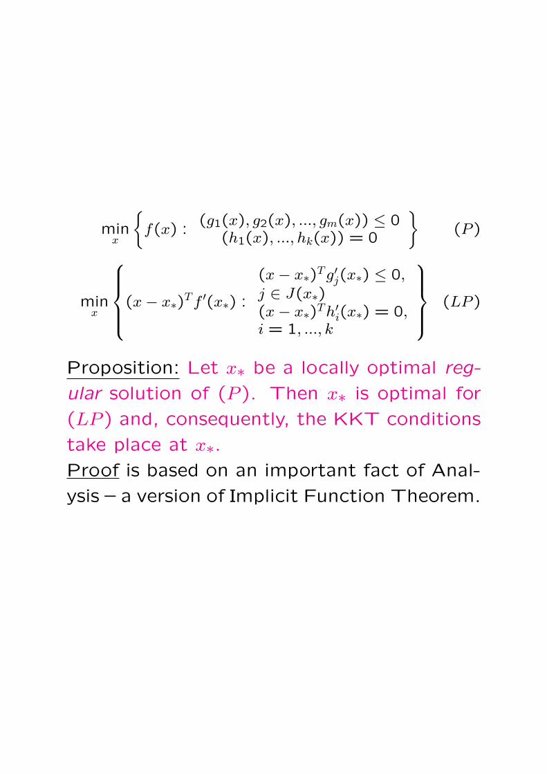
minx
f(x) :
(g1(x), g2(x), ..., gm(x)) ≤ 0(h1(x), ..., hk(x)) = 0
(P )
minx
(x− x∗)Tf ′(x∗) :
(x− x∗)Tg′j(x∗) ≤ 0,j ∈ J(x∗)(x− x∗)Th′i(x∗) = 0,i = 1, ..., k
(LP )
Proposition: Let x∗ be a locally optimal reg-
ular solution of (P ). Then x∗ is optimal for
(LP ) and, consequently, the KKT conditions
take place at x∗.Proof is based on an important fact of Anal-
ysis – a version of Implicit Function Theorem.

Theorem: Let x∗ ∈ Rn and let p`(x), ` =
1, ..., L, be real-valued functions such that
♦p` are κ ≥ 1 times continuously differen-
tiable in a neighbourhood of x∗♦p`(x∗) = 0
♦vectors ∇p`(x∗), ` = 1, ..., L, are linearly in-
dependent.
Then there exists substitution of variables
y 7→ x = Φ(y)
defined in a neighbourhood V of the origin
and mapping V , in a one-to-one manner,
onto a neighbourhood B of x∗, such that
♦x∗ = Φ(0
♦both Φ : V → B and its inverse mapping
Φ−1 : B → V are κ times continuously differ-
entiable
♦in coordinates y, the functions p` become
just the coordinates:
y ∈ V ⇒ p`(Φ(y)) ≡ y`, ` = 1, ..., L.
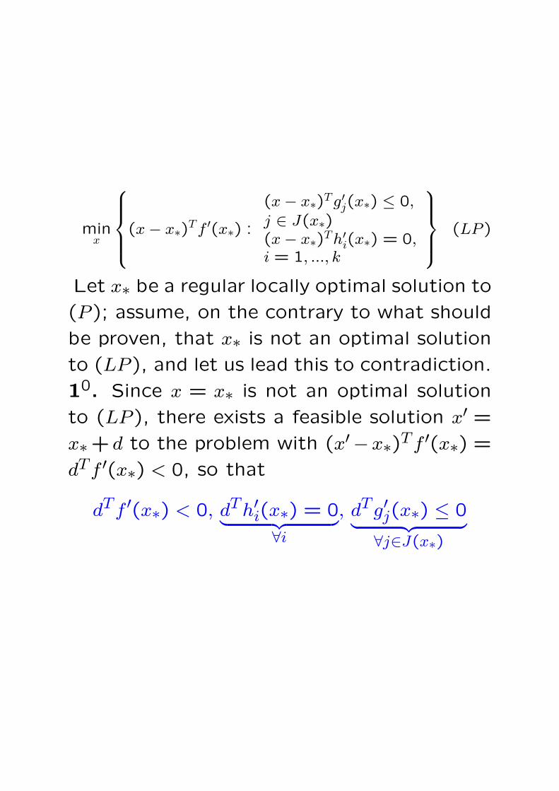
minx
(x− x∗)Tf ′(x∗) :
(x− x∗)Tg′j(x∗) ≤ 0,j ∈ J(x∗)(x− x∗)Th′i(x∗) = 0,i = 1, ..., k
(LP )
Let x∗ be a regular locally optimal solution to
(P ); assume, on the contrary to what should
be proven, that x∗ is not an optimal solution
to (LP ), and let us lead this to contradiction.
10. Since x = x∗ is not an optimal solution
to (LP ), there exists a feasible solution x′ =x∗+ d to the problem with (x′−x∗)Tf ′(x∗) =
dTf ′(x∗) < 0, so that
dTf ′(x∗) < 0, dTh′i(x∗) = 0︸ ︷︷ ︸∀i
, dTg′j(x∗) ≤ 0︸ ︷︷ ︸∀j∈J(x∗)
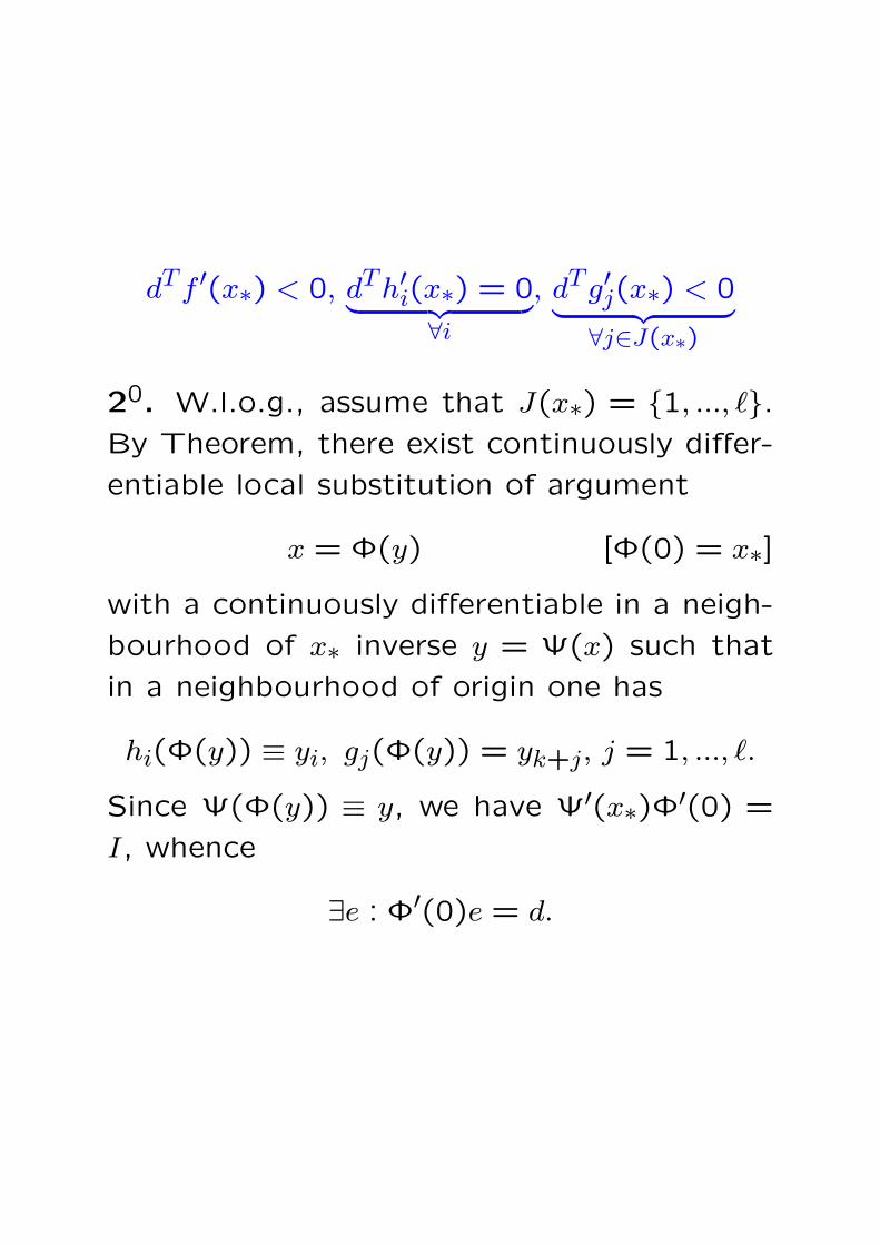
dTf ′(x∗) < 0, dTh′i(x∗) = 0︸ ︷︷ ︸∀i
, dTg′j(x∗) < 0︸ ︷︷ ︸∀j∈J(x∗)
20. W.l.o.g., assume that J(x∗) = 1, ..., `.By Theorem, there exist continuously differ-
entiable local substitution of argument
x = Φ(y) [Φ(0) = x∗]
with a continuously differentiable in a neigh-
bourhood of x∗ inverse y = Ψ(x) such that
in a neighbourhood of origin one has
hi(Φ(y)) ≡ yi, gj(Φ(y)) = yk+j, j = 1, ..., `.
Since Ψ(Φ(y)) ≡ y, we have Ψ′(x∗)Φ′(0) =
I, whence
∃e : Φ′(0)e = d.

Situation: We have found a smooth local sub-stitution of argument x = Φ(y) (y = 0 cor-responds to x = x∗) and a direction e suchthat in a neighbourhood of y = 0 one has
(a) hi(Φ(y)) ≡ yi, i ≤ k(b) gj(Φ(y)) ≡ yk+j, j ≤ `
[J(x∗) = 1, ..., `](c) [Φ′(0)e]Th′i(x∗) = 0, i ≤ k
(d) [Φ′(0)e]Tg′j(x∗) < 0, j ≤ `
(e) [Φ′(0)e]Tf ′(x∗) < 0
Consider the differentiable curve
x(t) = Φ(te).
We have
tei ≡ hi(Φ(te)) ⇒ ei = [Φ′(0)e]Th′i(x∗) = 0tek+j ≡ gj(Φ(te)) ⇒ ek+j = [Φ′(0)e]Tg′j(x∗) < 0
⇒ hi(x(t)) = tei = 0︸ ︷︷ ︸∀i
, gj(x(t)) = tek+j ≤ 0︸ ︷︷ ︸∀j∈J(x∗)
Thus, x(t) is feasible for all small t ≥ 0. But:
d
dt
∣∣∣t=0
f(x(t)) = [Φ′(0)e]Tf ′(x∗) < 0,
whence f(x(t)) < f(x(0)) = f(x∗) for allsmall enough t > 0, which is a contradictionwith local optimality of x∗.
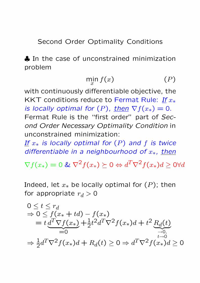
Second Order Optimality Conditions
♣ In the case of unconstrained minimizationproblem
minx
f(x) (P )
with continuously differentiable objective, theKKT conditions reduce to Fermat Rule: If x∗is locally optimal for (P ), then ∇f(x∗) = 0.
Fermat Rule is the “first order” part of Sec-ond Order Necessary Optimality Condition inunconstrained minimization:If x∗ is locally optimal for (P ) and f is twicedifferentiable in a neighbourhood of x∗, then
∇f(x∗) = 0 & ∇2f(x∗) º 0 ⇔ dT∇2f(x∗)d ≥ 0∀d
Indeed, let x∗ be locally optimal for (P ); thenfor appropriate rd > 0
0 ≤ t ≤ rd⇒ 0 ≤ f(x∗ + td)− f(x∗)
= t dT∇f(x∗)︸ ︷︷ ︸=0
+12t2dT∇2f(x∗)d + t2 Rd(t)︸ ︷︷ ︸
→0,t→0
⇒ 12dT∇2f(x∗)d + Rd(t) ≥ 0 ⇒ dT∇2f(x∗)d ≥ 0

minx
f(x) (P )
The necessary Second Order Optimality con-dition in unconstrained minimization can bestrengthened toSecond Order Sufficient Optimality Conditionin unconstrained minimization: Let f betwice differentiable in a neighbourhood of x∗.If
∇f(x∗) = 0,∇2f(x∗) Â 0 ⇔ dT∇2f(x∗)d > 0∀d 6= 0
then x∗ is locally optimal for (P ).Proof: Since dT∇2f(x∗)d > 0 for all d > 0,then there exists α > 0 such that dT∇2f(x∗)d ≥αdTd for all d.By differentiability, for every ε > 0 there ex-ists rε > 0 such that
‖d‖2 ≤ rε
⇒ f(x∗ + d)− f(x∗) ≥ dT∇f(x∗)︸ ︷︷ ︸=0
+12 dT∇2f(x∗)d︸ ︷︷ ︸
≥αdT d
− ε2dTd
⇒ f(x∗ + d)− f(x∗) ≥ 12(α− ε)dTd
Setting ε = α2, we see that x∗ is a local mini-
mizer of f .

We are given a Mathematical Programmingproblem
minx
f(x) :
(g1(x), g2(x), ..., gm(x)) ≤ 0(h1(x), ..., hk(x)) = 0
(P )
⇓L(x;λ, µ) = f(x) +
∑j
λjgj(x) +∑i
µihi(x)
♣ In Optimality Conditions for a constrainedproblem (P ), the role of ∇2f(x∗) is played bythe Hessian of the Lagrange function:Second Order Necessary Optimality Condition:Let x∗ be a regular feasible solution of (P )such that the functions f, gj, hi are twice con-tinuously differentiable in a neighbourhood ofx∗. If x∗ is locally optimal, then♦There exist uniquely defined Lagrange mul-tipliers λ∗j ≥ 0, µ∗i such that the KKT condi-tions hold:
∇xL(x∗;λ∗, µ∗) = 0λ∗jgj(x∗) = 0, j = 1, ..., m
♦For every d orthogonal to the gradients,taken at x∗, of all active at x∗ equality andinequality constraints, one has
dT∇2xL(x∗;λ∗, µ∗)d ≥ 0.


Proof. 10. Constraints which are non-active
at x∗ clearly do not affect neither local opti-
mality of x∗, nor the conclusion to be proven.
Removing these constraints, we reduce the
situation to one where all constraints in the
problem
minx
f(x) :
(g1(x), g2(x), ..., gm(x)) ≤ 0(h1(x), ..., hk(x)) = 0
(P )
are active at x∗.20. Applying Implicit Function Theorem, we
can find a local change of variables
x = Φ(y) ⇔ y = Ψ(x)
[Φ(0) = x∗,Ψ(x∗) = 0]
with locally twice continuously differentiable
Φ,Ψ such that
gj(Φ(y)) ≡ yj, j ≤ m, hi(Φ(y)) ≡ ym+i, i ≤ k.
In variables y, problem (P ) becomes
miny
f(Φ(y))︸ ︷︷ ︸
φ(y)
: yj ≤ 0, j ≤ m, yk+i = 0, i ≤ k
.
(P ′)

minx
f(x) :
(g1(x), g2(x), ..., gm(x)) ≤ 0(h1(x), ..., hk(x)) = 0
(P )
m [x = Φ(y)]
miny
f(Φ(y))︸ ︷︷ ︸
φ(y)
: yj ≤ 0, j ≤ m, yk+i = 0, i ≤ k
(P ′)
⇓M(y;λ, µ) = φ(y) +
∑j
λjyj +∑i
µiym+i
Our plan is as follows:
♦Since Φ is a smooth one-to-one mapping
of a neighbourhood of x∗ onto a neighbour-
hood of y∗ = 0, x∗ is locally optimal for (P )
iff y∗ = 0 is locally optimal for (P ′).♦We intend to build necessary/sufficient con-
ditions for y∗ = 0 to be locally optimal for
(P ′); “translated” to x-variables, these con-
ditions will imply necessary/sufficient condi-
tions for local optimality of x∗ for (P ).
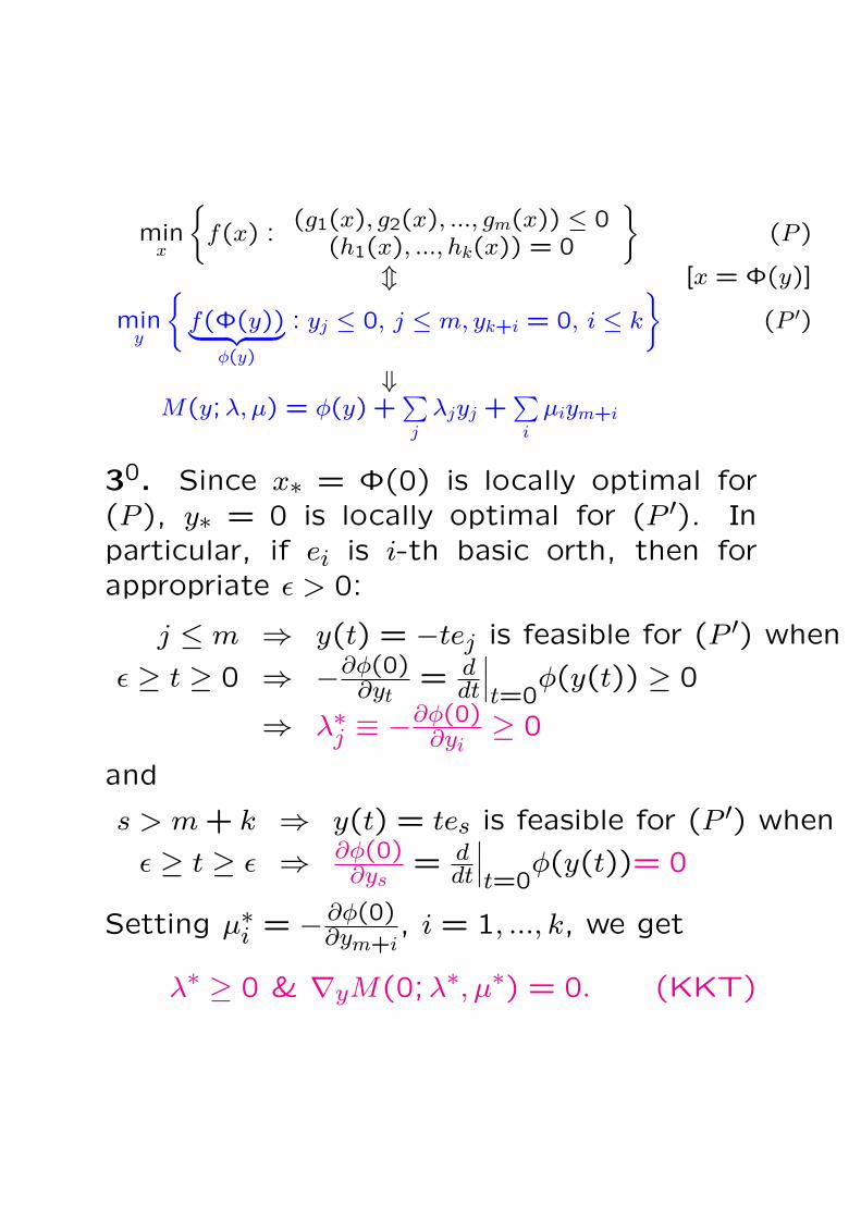
minx
f(x) :
(g1(x), g2(x), ..., gm(x)) ≤ 0(h1(x), ..., hk(x)) = 0
(P )
m [x = Φ(y)]
miny
f(Φ(y))︸ ︷︷ ︸
φ(y)
: yj ≤ 0, j ≤ m, yk+i = 0, i ≤ k
(P ′)
⇓M(y;λ, µ) = φ(y) +
∑j
λjyj +∑i
µiym+i
30. Since x∗ = Φ(0) is locally optimal for(P ), y∗ = 0 is locally optimal for (P ′). Inparticular, if ei is i-th basic orth, then forappropriate ε > 0:
j ≤ m ⇒ y(t) = −tej is feasible for (P ′) when
ε ≥ t ≥ 0 ⇒ −∂φ(0)∂yt
= ddt
∣∣∣t=0
φ(y(t)) ≥ 0
⇒ λ∗j ≡ −∂φ(0)∂yi
≥ 0
and
s > m + k ⇒ y(t) = tes is feasible for (P ′) when
ε ≥ t ≥ ε ⇒ ∂φ(0)∂ys
= ddt
∣∣∣t=0
φ(y(t))= 0
Setting µ∗i = − ∂φ(0)∂ym+i
, i = 1, ..., k, we get
λ∗ ≥ 0 & ∇yM(0;λ∗, µ∗) = 0. (KKT)
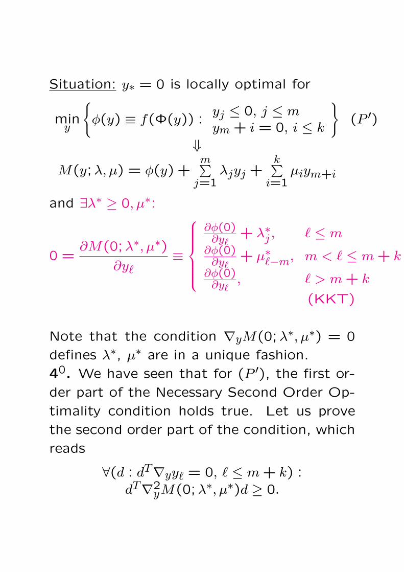
Situation: y∗ = 0 is locally optimal for
miny
φ(y) ≡ f(Φ(y)) :
yj ≤ 0, j ≤ mym + i = 0, i ≤ k
(P ′)
⇓M(y;λ, µ) = φ(y) +
m∑j=1
λjyj +k∑
i=1µiym+i
and ∃λ∗ ≥ 0, µ∗:
0 =∂M(0;λ∗, µ∗)
∂y`≡
∂φ(0)∂y`
+ λ∗j , ` ≤ m∂φ(0)∂y`
+ µ∗`−m, m < ` ≤ m + k∂φ(0)∂y`
, ` > m + k
(KKT)
Note that the condition ∇yM(0;λ∗, µ∗) = 0
defines λ∗, µ∗ are in a unique fashion.
40. We have seen that for (P ′), the first or-
der part of the Necessary Second Order Op-
timality condition holds true. Let us prove
the second order part of the condition, which
reads
∀(d : dT∇yy` = 0, ` ≤ m + k) :dT∇2
yM(0;λ∗, µ∗)d ≥ 0.

Situation: y∗ = 0 is locally optimal solutionto the problem
miny
φ(y) ≡ f(Φ(y)) :
yj ≤ 0, j ≤ mym + i = 0, i ≤ k
(P ′)Claim:
∀(d : dT∇yy` = 0, ` ≤ m + k) :dT∇2
yM(0;λ∗, µ∗)d ≥ 0.
This is evident: since M(y;λ∗, µ∗) = φ(y) +m∑
j=1λ∗jyj +
k∑i=1
µ∗i ym+i, we have
∇2yM(0;λ∗, µ∗) = ∇2φ(0).
Claim therefore states that dT∇2φ(0)d ≥ 0for every vector d from the linear subspaceL = d : d1 = ... = dm+k = 0. But thissubspace is feasible for (P ′), so that φ, re-stricted onto L, should attain unconstrainedlocal minimum at the origin. By NecessarySecond Order Optimality condition for un-constrained minimization,
dT∇2φ(0)d ≥ 0 ∀d ∈ L.
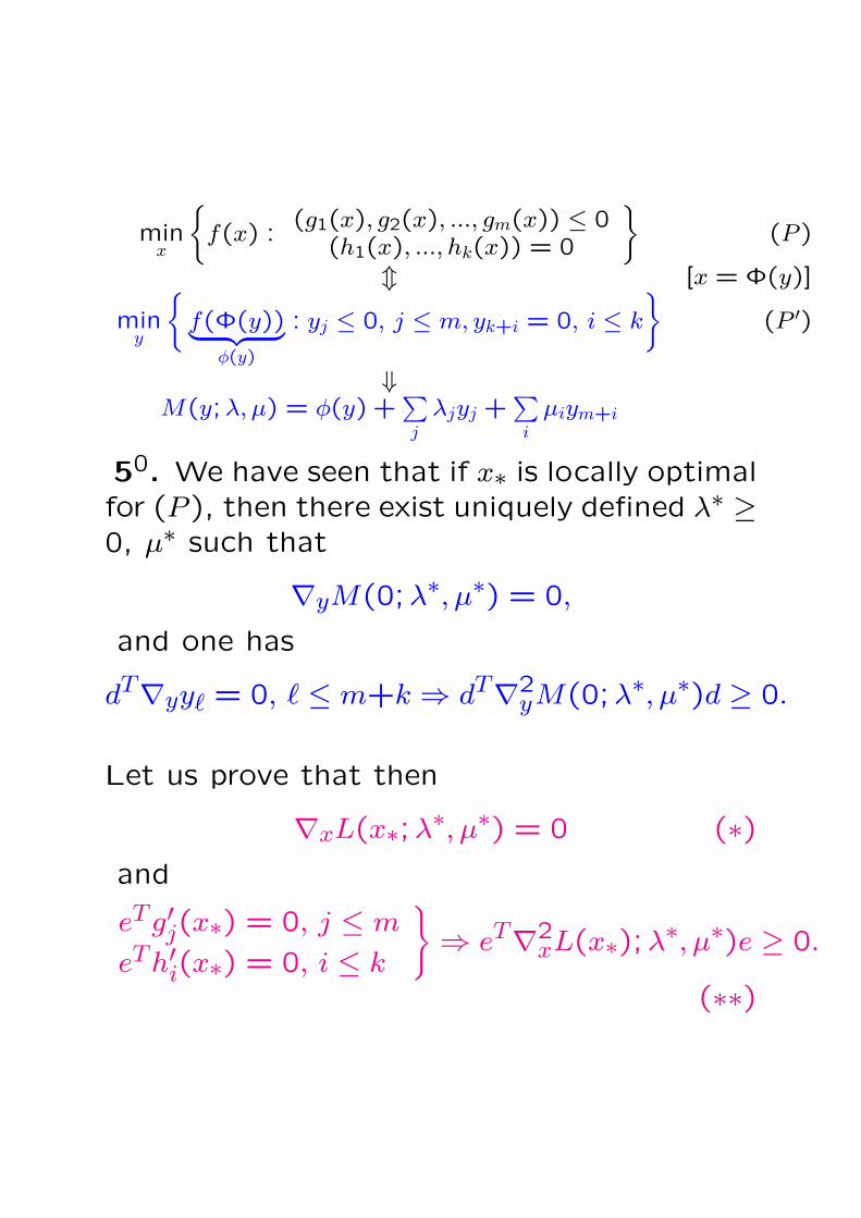
minx
f(x) :
(g1(x), g2(x), ..., gm(x)) ≤ 0(h1(x), ..., hk(x)) = 0
(P )
m [x = Φ(y)]
miny
f(Φ(y))︸ ︷︷ ︸
φ(y)
: yj ≤ 0, j ≤ m, yk+i = 0, i ≤ k
(P ′)
⇓M(y;λ, µ) = φ(y) +
∑j
λjyj +∑i
µiym+i
50. We have seen that if x∗ is locally optimalfor (P ), then there exist uniquely defined λ∗ ≥0, µ∗ such that
∇yM(0;λ∗, µ∗) = 0,
and one has
dT∇yy` = 0, ` ≤ m+k ⇒ dT∇2yM(0;λ∗, µ∗)d ≥ 0.
Let us prove that then
∇xL(x∗;λ∗, µ∗) = 0 (∗)and
eTg′j(x∗) = 0, j ≤ m
eTh′i(x∗) = 0, i ≤ k
⇒ eT∇2
xL(x∗);λ∗, µ∗)e ≥ 0.
(∗∗)

Given:
∇yM(0;λ∗, µ∗) = 0dT∇yy` = 0, ` ≤ m + k ⇒ dT∇2
yM(0;λ∗, µ∗)d ≥ 0.
Should prove:
∇xL(x∗;λ∗, µ∗) = 0 (∗)eTg′j(x∗) = 0, j ≤ m
eTh′i(x∗) = 0, i ≤ k
⇒ eT∇2
xL(x∗);λ∗, µ∗)e ≥ 0 (∗∗)
♦Setting L(x) = L(x;λ∗, µ∗), M(y) = M(y;λ∗, µ∗),we have
L(x) = M(Ψ(x))⇒ ∇xL(x∗) = [Ψ′(x∗)]T∇yM(y∗) = 0,
as required in (∗).♦Let e satisfy the premise in (∗∗), and letd = [Φ′(0)]−1e. Then
ddt
∣∣∣t=0
tdj︷ ︸︸ ︷d
dt
∣∣∣∣∣t=0
gj(Φ(td)) = [g′j(x∗)]Te︷ ︸︸ ︷
[Φ′(0)]d
⇒ dj = eTg′j(x∗) = 0, j ≤ m
d
dt
∣∣∣∣∣t=0
hi(Φ(td))
︸ ︷︷ ︸ddt
∣∣∣t=0
tdm+i
= [h′i(x∗)]T [Φ′(0)]d︸ ︷︷ ︸e
⇒ dm+i = eTh′i(x∗) = 0, i ≤ k
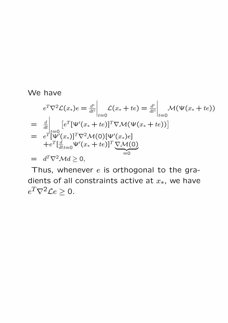
We have
eT∇2L(x∗)e = d2
dt2
∣∣∣∣t=0
L(x∗ + te) = d2
dt2
∣∣∣∣t=0
M(Ψ(x∗ + te))
= ddt
∣∣∣∣t=0
[eT [Ψ′(x∗ + te)]T∇M(Ψ(x∗ + te))
]
= eT [Ψ′(x∗)]T∇2M(0)[Ψ′(x∗)e]+eT [ d
dtt=0Ψ′(x∗ + te)]T ∇M(0)︸ ︷︷ ︸
=0= dT∇2Md ≥ 0,
Thus, whenever e is orthogonal to the gra-
dients of all constraints active at x∗, we have
eT∇2Le ≥ 0.

Second Order Sufficient Condition for LocalOptimality
minx
f(x) :
(g1(x), g2(x), ..., gm(x)) ≤ 0(h1(x), ..., hk(x)) = 0
(P )
⇓L(x;λ, µ) = f(x) +
∑j
λjgj(x) +∑i
µihi(x)
Second Order Sufficient Optimality Condition:Let x∗ be a regular feasible solution of (P )such that the functions f, gj, hi are twice con-tinuously differentiable in a neighbourhood ofx∗. If there exist Lagrange multipliers λ∗j ≥ 0,µ∗i such that♦the KKT conditions hold:
∇xL(x∗;λ∗, µ∗) = 0λ∗jgj(x∗) = 0, j = 1, ..., m
♦For every d 6= 0 orthogonal to the gradi-ents, taken at x∗, of all active at x∗ equalityconstraints and those active at x∗ inequalityconstraints for which λ∗j > 0, one has
dT∇2xL(x∗;λ∗, µ∗)d > 0
then x∗ is locally optimal for (P ).
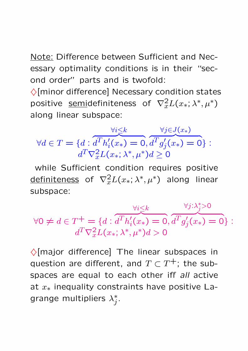
Note: Difference between Sufficient and Nec-
essary optimality conditions is in their “sec-
ond order” parts and is twofold:
♦[minor difference] Necessary condition states
positive semidefiniteness of ∇2xL(x∗;λ∗, µ∗)
along linear subspace:
∀d ∈ T = d :
∀i≤k︷ ︸︸ ︷dTh′i(x∗) = 0,
∀j∈J(x∗)︷ ︸︸ ︷dTg′j(x∗) = 0 :
dT∇2xL(x∗;λ∗, µ∗)d ≥ 0
while Sufficient condition requires positive
definiteness of ∇2xL(x∗;λ∗, µ∗) along linear
subspace:
∀0 6= d ∈ T+ = d :
∀i≤k︷ ︸︸ ︷dTh′i(x∗) = 0,
∀j:λ∗j>0︷ ︸︸ ︷dTg′j(x∗) = 0 :
dT∇2xL(x∗;λ∗, µ∗)d > 0
♦[major difference] The linear subspaces in
question are different, and T ⊂ T+; the sub-
spaces are equal to each other iff all active
at x∗ inequality constraints have positive La-
grange multipliers λ∗j .
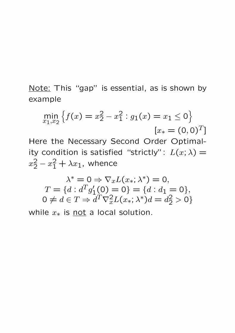
Note: This “gap” is essential, as is shown by
example
minx1,x2
f(x) = x2
2 − x21 : g1(x) = x1 ≤ 0
[x∗ = (0,0)T ]
Here the Necessary Second Order Optimal-
ity condition is satisfied “strictly”: L(x;λ) =
x22 − x2
1 + λx1, whence
λ∗ = 0 ⇒ ∇xL(x∗;λ∗) = 0,
T = d : dTg′1(0) = 0 = d : d1 = 0,0 6= d ∈ T ⇒ dT∇2
xL(x∗;λ∗)d = d22 > 0
while x∗ is not a local solution.

Proof of Sufficient Second Order Opti-
mality Condition. 10. As in the case of Sec-
ond Order Necessary Optimality Condition,
we can reduce the situation to one where
♦All inequality constraints are active at x∗♦The problem is of the special form
miny
φ(y) :
yj ≤ 0, j ≤ mym+i = 0, i ≤ k
(P ′)
20. In the case of (P ′), Sufficient conditionreads: ∃λ∗ ≥ 0, µ∗:
∇y
∣∣y=0
φ(y) +
m∑j=1
λ∗jyj +k∑
i=1µ∗i ym+i
dj = 0, j ∈ J, d 6= 0 ⇒ dT∇2φ(0)d > 0[J = j ≤ m : λ∗j > 0 ∪ m + 1, ..., m + k]
(∗)
Assuming w.l.o.g. j : λ∗j > 0 = 1, ..., q, (∗) reads:
∂φ(0)∂y`
< 0, ` = 1, ..., q∂φ(0)
∂y`= 0, ` = q + 1, ..., m
∂φ(0)∂y`
= 0, ` = m + k + 1, ..., n
0 6= d ∈ T+ = d : d` = 0, ` ∈ 1, ..., q, m + 1, ..., m + k :⇒ dT∇2φ(0)d > 0
Our goal is to derive from this assumption local opti-mality of y∗ = 0 for (P ′).

20. The feasible set of (P ′) is the closedcone
K = d : d` ≤ 0, ` = 1, ..., m, d` = 0, ` = m+1, ..., m+k
Lemma: For 0 6= d ∈ K one has dT∇φ(0) ≥ 0
and
dT∇φ(0) = 0 ⇒ dT∇2φ(0)d > 0.
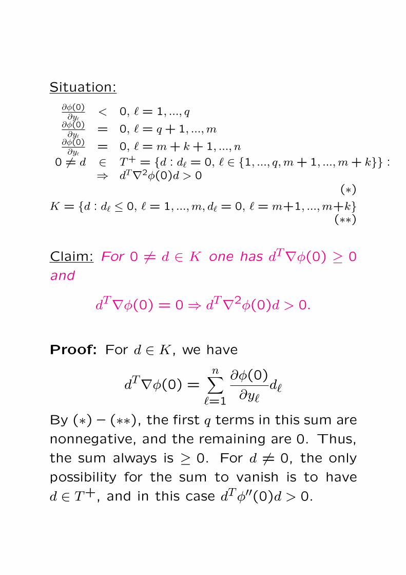
Situation:
∂φ(0)∂y`
< 0, ` = 1, ..., q∂φ(0)
∂y`= 0, ` = q + 1, ..., m
∂φ(0)∂y`
= 0, ` = m + k + 1, ..., n
0 6= d ∈ T+ = d : d` = 0, ` ∈ 1, ..., q, m + 1, ..., m + k :⇒ dT∇2φ(0)d > 0
(∗)K = d : d` ≤ 0, ` = 1, ..., m, d` = 0, ` = m+1, ..., m+k
(∗∗)
Claim: For 0 6= d ∈ K one has dT∇φ(0) ≥ 0
and
dT∇φ(0) = 0 ⇒ dT∇2φ(0)d > 0.
Proof: For d ∈ K, we have
dT∇φ(0) =n∑
`=1
∂φ(0)
∂y`d`
By (∗) – (∗∗), the first q terms in this sum are
nonnegative, and the remaining are 0. Thus,
the sum always is ≥ 0. For d 6= 0, the only
possibility for the sum to vanish is to have
d ∈ T+, and in this case dTφ′′(0)d > 0.
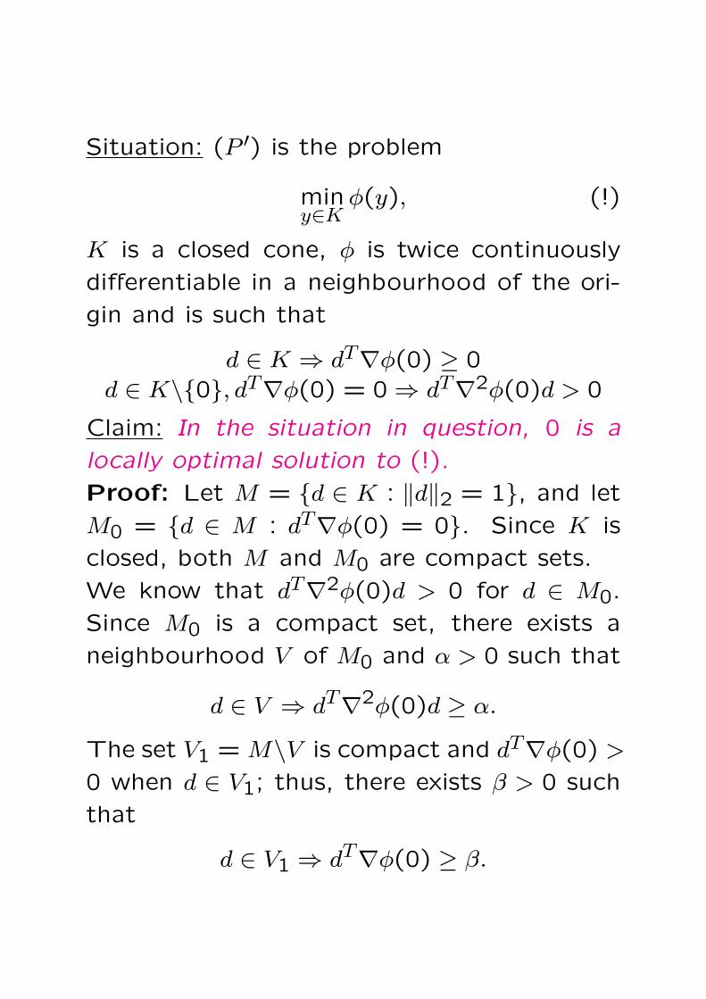
Situation: (P ′) is the problem
miny∈K
φ(y), (!)
K is a closed cone, φ is twice continuously
differentiable in a neighbourhood of the ori-
gin and is such that
d ∈ K ⇒ dT∇φ(0) ≥ 0d ∈ K\0, dT∇φ(0) = 0 ⇒ dT∇2φ(0)d > 0
Claim: In the situation in question, 0 is a
locally optimal solution to (!).
Proof: Let M = d ∈ K : ‖d‖2 = 1, and let
M0 = d ∈ M : dT∇φ(0) = 0. Since K is
closed, both M and M0 are compact sets.
We know that dT∇2φ(0)d > 0 for d ∈ M0.
Since M0 is a compact set, there exists a
neighbourhood V of M0 and α > 0 such that
d ∈ V ⇒ dT∇2φ(0)d ≥ α.
The set V1 = M\V is compact and dT∇φ(0) >
0 when d ∈ V1; thus, there exists β > 0 such
that
d ∈ V1 ⇒ dT∇φ(0) ≥ β.

Situation: K is a cone, and the set M = d ∈K : ‖d‖2 = 1 is partitioned into two subsets
V0 = V ∩M and V1 in such a way that
d ∈ V0 ⇒ dT∇φ(0) ≥ 0, dT∇2φ(0)d ≥ α > 0d ∈ V1 → dT∇φ(0) ≥ β > 0
Goal: To prove that 0 is local minimizer of φ
on K, or, which is the same, that
∃r > 0 :φ(0) ≤ φ(td) ∀(d ∈ M,0 ≤ t ≤ r).
Proof: Let d ∈ M , t ≥ 0. When d ∈ V0, wehave
φ(td)− φ(0) ≥ tdT∇φ(0) + 12t2dT∇2φ(0)d− t2 R(t)︸ ︷︷ ︸
→0,
t→+0
≥ 12t2(α− 2R(t))
⇒ ∃r0 > 0 : φ(td)− φ(0) ≥ 14t2α ≥ 0 ∀t ≤ r0
When d ∈ V1, we have
φ(td)− φ(0) ≥ tdT∇φ(0) + 12t2dT∇2φ(0)d− t2 R(t)︸ ︷︷ ︸
→0,
t→+0
≥ βt− Ct2 − t2R(t)⇒ ∃r1 > 0 : φ(td)− φ(0) ≥ β
2t ≥ 0∀t ≤ r1
Thus, φ(td)−φ(0) ≥ 0 for all t ≤ min[r0, r1],
d ∈ M .
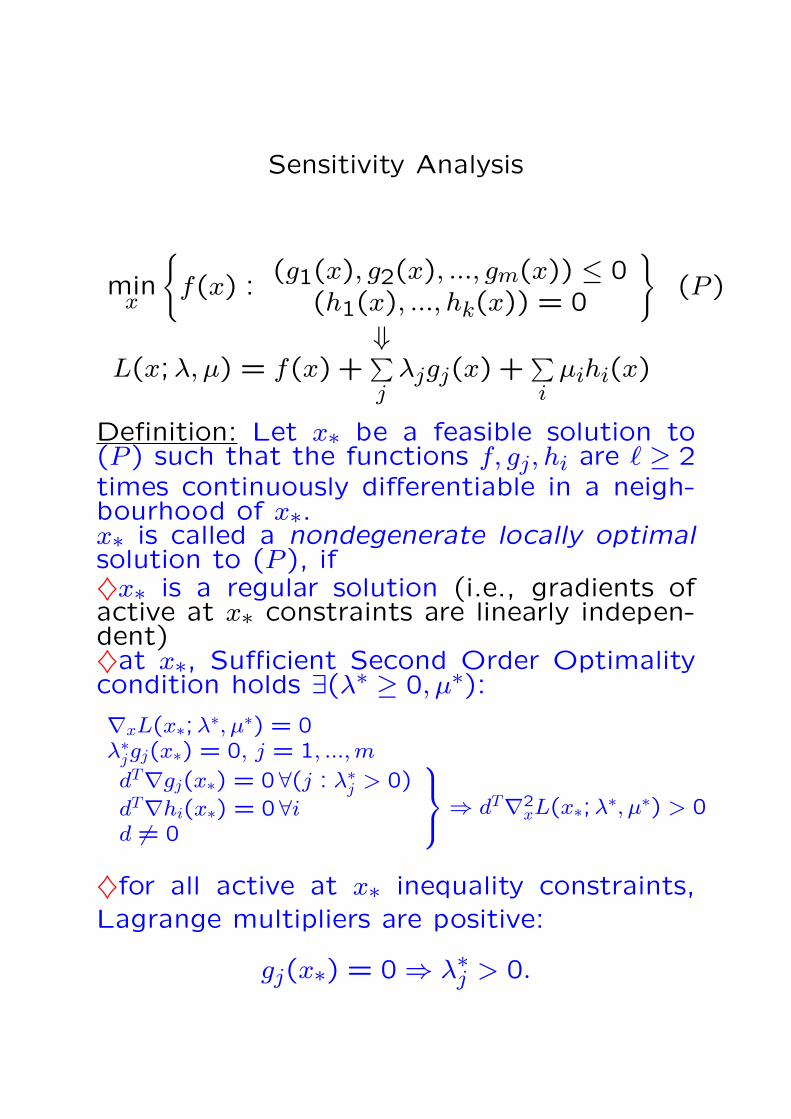
Sensitivity Analysis
minx
f(x) :
(g1(x), g2(x), ..., gm(x)) ≤ 0(h1(x), ..., hk(x)) = 0
(P )
⇓L(x;λ, µ) = f(x) +
∑j
λjgj(x) +∑i
µihi(x)
Definition: Let x∗ be a feasible solution to(P ) such that the functions f, gj, hi are ` ≥ 2times continuously differentiable in a neigh-bourhood of x∗.x∗ is called a nondegenerate locally optimalsolution to (P ), if♦x∗ is a regular solution (i.e., gradients ofactive at x∗ constraints are linearly indepen-dent)♦at x∗, Sufficient Second Order Optimalitycondition holds ∃(λ∗ ≥ 0, µ∗):∇xL(x∗;λ∗, µ∗) = 0λ∗jgj(x∗) = 0, j = 1, ..., m
dT∇gj(x∗) = 0 ∀(j : λ∗j > 0)dT∇hi(x∗) = 0 ∀id 6= 0
⇒ dT∇2
xL(x∗;λ∗, µ∗) > 0
♦for all active at x∗ inequality constraints,Lagrange multipliers are positive:
gj(x∗) = 0 ⇒ λ∗j > 0.


minx
f(x) :
(g1(x), g2(x), ..., gm(x)) ≤ 0(h1(x), ..., hk(x)) = 0
(P )
Theorem: Let x∗ be a nondegenerate locallyoptimal solution to (P ). Let us embed (P )into the parametric family of problems
minx
f(x) :
g1(x) ≤ a1, ..., gm(x) ≤ am
h1(x) = b1, ..., hk(x) = bk
(P [a, b])
so that (P ) is (P [0,0]).There exists a neighbourhood Vx of x∗ and aneighbourhood Va,b of the point a = 0, b = 0in the space of parameters a, b such that♦∀(a, b) ∈ Va,b, in Vv there exists a uniqueKKT point x∗(a, b) of (P [a, b]), and this pointis a nondegenerate locally optimal solutionto (P [a, b]); moreover, x∗(a, b) is optimal so-lution for the optimization problem
Optloc(a, b) = minx
f(x) :
g1(x) ≤ a1, ..., gm(x) ≤ am
h1(x) = b1, ..., hk(x) = bk
x ∈ Vx
(Ploc[a, b])

♦both x∗(a, b) and the corresponding La-
grange multipliers λ∗(a, b), µ∗(a, b) are ` − 1
times continuously differentiable functions of
(a, b) ∈ Va,b, and
∂Optloc(a,b)∂aj
= ∂f(x∗(a,b))∂aj
= −λ∗j(a, b)
∂Optloc(a,b)∂bi
= ∂f(x∗(a,b))∂bi
= −µ∗i (a, b)
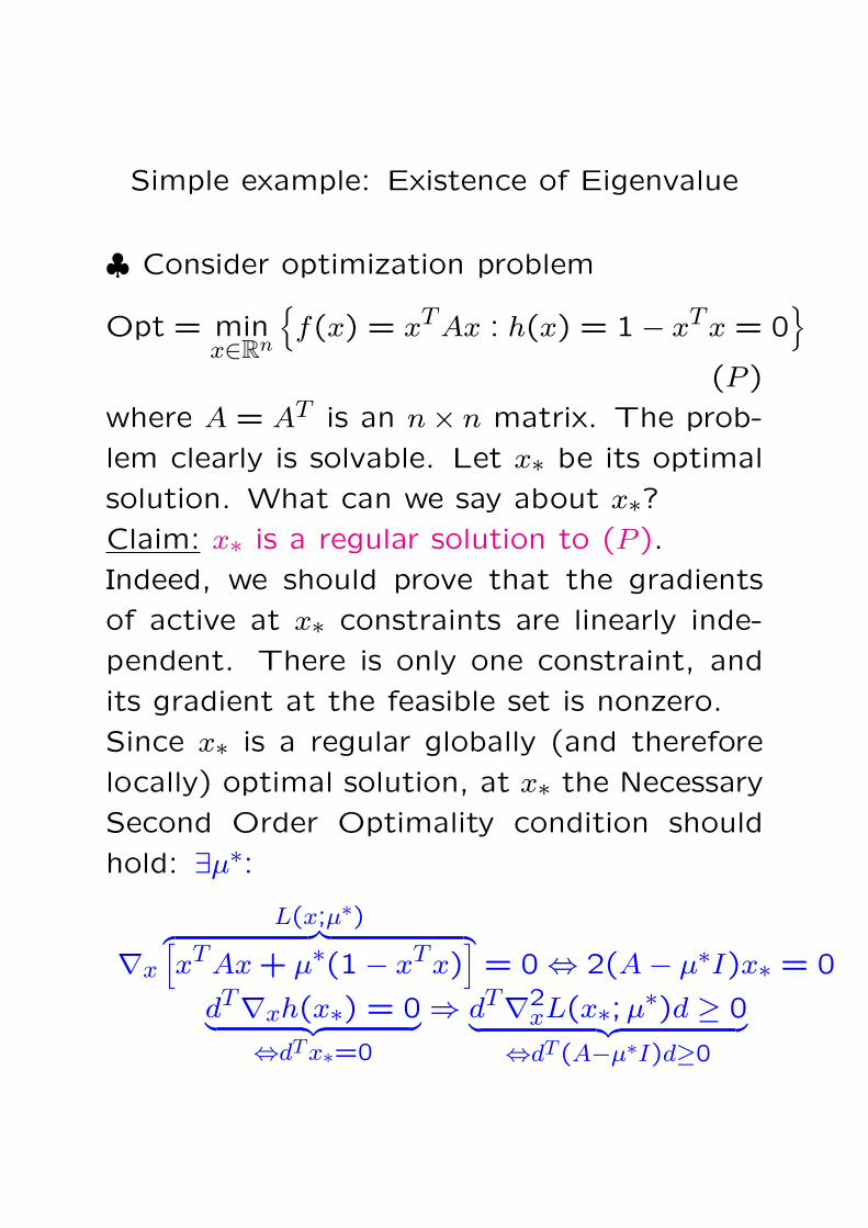
Simple example: Existence of Eigenvalue
♣ Consider optimization problem
Opt = minx∈Rn
f(x) = xTAx : h(x) = 1− xTx = 0
(P )
where A = AT is an n× n matrix. The prob-
lem clearly is solvable. Let x∗ be its optimal
solution. What can we say about x∗?Claim: x∗ is a regular solution to (P ).
Indeed, we should prove that the gradients
of active at x∗ constraints are linearly inde-
pendent. There is only one constraint, and
its gradient at the feasible set is nonzero.
Since x∗ is a regular globally (and therefore
locally) optimal solution, at x∗ the Necessary
Second Order Optimality condition should
hold: ∃µ∗:
∇x
L(x;µ∗)︷ ︸︸ ︷[xTAx + µ∗(1− xTx)
]= 0 ⇔ 2(A− µ∗I)x∗ = 0
dT∇xh(x∗) = 0︸ ︷︷ ︸⇔dT x∗=0
⇒ dT∇2xL(x∗;µ∗)d ≥ 0︸ ︷︷ ︸
⇔dT (A−µ∗I)d≥0
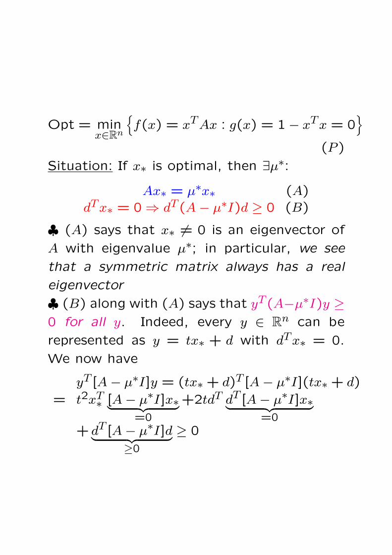
Opt = minx∈Rn
f(x) = xTAx : g(x) = 1− xTx = 0
(P )
Situation: If x∗ is optimal, then ∃µ∗:Ax∗ = µ∗x∗ (A)
dTx∗ = 0 ⇒ dT (A− µ∗I)d ≥ 0 (B)
♣ (A) says that x∗ 6= 0 is an eigenvector of
A with eigenvalue µ∗; in particular, we see
that a symmetric matrix always has a real
eigenvector
♣ (B) along with (A) says that yT (A−µ∗I)y ≥0 for all y. Indeed, every y ∈ Rn can be
represented as y = tx∗ + d with dTx∗ = 0.
We now have
yT [A− µ∗I]y = (tx∗ + d)T [A− µ∗I](tx∗ + d)
= t2xT∗ [A− µ∗I]x∗︸ ︷︷ ︸=0
+2tdT dT [A− µ∗I]x∗︸ ︷︷ ︸=0
+ dT [A− µ∗I]d︸ ︷︷ ︸≥0
≥ 0

Opt = minx∈Rn
f(x) = xTAx : g(x) = 1− xTx = 0
(P )
Note: In the case in question, Necessary
Second Order Optimality conditions can be
rewritten equivalently as ∃µ∗:[A− µ∗I]x∗ = 0
yT [A− µ∗I]y ≥ 0 ∀y (∗)
and are not only necessary, but also sufficient
for feasible solution x∗ to be globally optimal.
To prove sufficiency, let x∗ be feasible, and
µ∗ be such that (∗) holds true. For every
feasible solution x, one has
0 ≤ xT [A−µ∗I]x = xTAx−µ∗xTx = xTAx−µ∗,
whence xTAx ≥ µ∗. For x = x∗, we have
0 = xT∗ [A−µ∗I]x∗ = xT∗Ax∗−µ∗xT∗ x∗ = xT∗Ax∗−µ∗,
whence xT∗Ax∗ = µ∗. Thus, x∗ is globally
optimal for (P ), and µ∗ is the optimal value
in (P ).
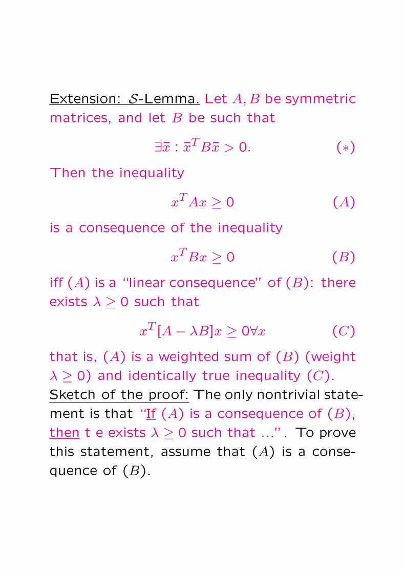
Extension: S-Lemma. Let A, B be symmetric
matrices, and let B be such that
∃x : xTBx > 0. (∗)Then the inequality
xTAx ≥ 0 (A)
is a consequence of the inequality
xTBx ≥ 0 (B)
iff (A) is a “linear consequence” of (B): there
exists λ ≥ 0 such that
xT [A− λB]x ≥ 0∀x (C)
that is, (A) is a weighted sum of (B) (weight
λ ≥ 0) and identically true inequality (C).
Sketch of the proof: The only nontrivial state-
ment is that “If (A) is a consequence of (B),
then t e exists λ ≥ 0 such that ...”. To prove
this statement, assume that (A) is a conse-
quence of (B).
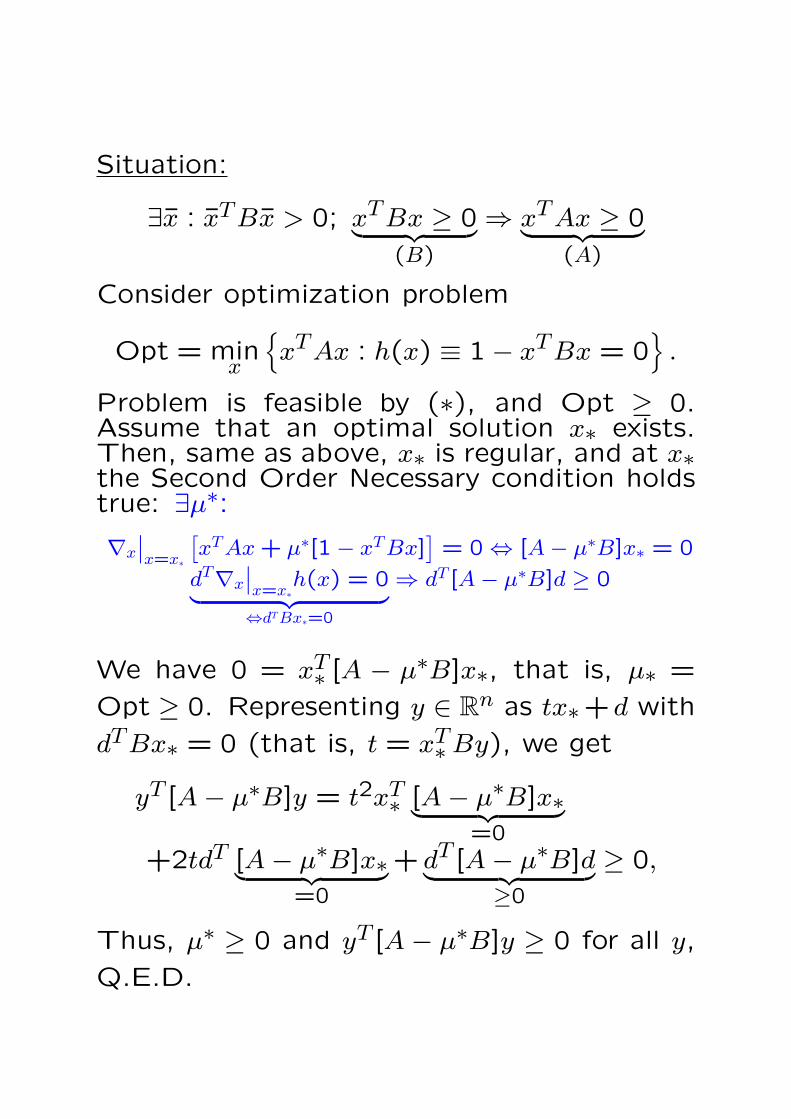
Situation:
∃x : xTBx > 0; xTBx ≥ 0︸ ︷︷ ︸(B)
⇒ xTAx ≥ 0︸ ︷︷ ︸(A)
Consider optimization problem
Opt = minx
xTAx : h(x) ≡ 1− xTBx = 0
.
Problem is feasible by (∗), and Opt ≥ 0.Assume that an optimal solution x∗ exists.Then, same as above, x∗ is regular, and at x∗the Second Order Necessary condition holdstrue: ∃µ∗:∇x
∣∣x=x∗
[xTAx + µ∗[1− xTBx]
]= 0 ⇔ [A− µ∗B]x∗ = 0
dT∇x
∣∣x=x∗
h(x) = 0︸ ︷︷ ︸⇔dTBx∗=0
⇒ dT [A− µ∗B]d ≥ 0
We have 0 = xT∗ [A − µ∗B]x∗, that is, µ∗ =
Opt ≥ 0. Representing y ∈ Rn as tx∗+d with
dTBx∗ = 0 (that is, t = xT∗By), we get
yT [A− µ∗B]y = t2xT∗ [A− µ∗B]x∗︸ ︷︷ ︸=0
+2tdT [A− µ∗B]x∗︸ ︷︷ ︸=0
+ dT [A− µ∗B]d︸ ︷︷ ︸≥0
≥ 0,
Thus, µ∗ ≥ 0 and yT [A− µ∗B]y ≥ 0 for all y,
Q.E.D.

Introduction to Optimization Algorithms
♣ Goal: Approximate numerically solutions to
Mathematical Programming problems
minx
f(x) :
gj(x) ≤ 0, j = 1, ..., mhi(x) = 0, i = 1, ..., k
(P )
♣ Traditional MP algorithms to be consid-
ered in the Course do not assume the analytic
structure of (P ) to be known in advance (and
do not know how to use the structure when it
is known). These algorithms are black-box-
oriented: when solving (P ), method gener-
ates a sequence of iterates x1, x2,... in such
a way that xt+1 depends solely on local infor-
mation of (P ) gathered along the preceding
iterates x1, ..., xt.
Information on (P ) obtained at xt usually is
comprised of the values and the first and the
second derivatives of the objective and the
constraints at xt.
♠ Note: In optimization, there exist algo-
rithms which do exploit problem’s structure.
Traditional methods of this type – Simplex
method and its variations – do not go be-
yond Linear Programming and Linearly Con-
strained Quadratic Programming.
Recently, new efficient ways to exploit prob-
lem’s structure were discovered (Interior Point
methods). The resulting algorithms, how-
ever, do not go beyond Convex Program-
ming.

♣ Except for very specific and relatively sim-
ple problem classes, like Linear Programming
or Linearly Constrained Quadratic Program-
ming, optimization algorithms cannot guar-
antee finding exact solution – local or global
– in finite time. The best we can expect
from these algorithms is convergence of ap-
proximate solutions generated by algorithms
to the exact solutions.
♠ Even in the case when “finite” solution
methods do exist (Simplex method in Lin-
ear Programming), no reasonable complexity
bounds for these methods are known, there-
fore in reality the ability of a method to gen-
erate the exact solution in finitely many steps
is neither necessary, nor sufficient to justify
the method.

♣ Aside of Convex Programming, traditionaloptimization methods are unable to guaran-tee convergence to a globally optimal solu-tion. Indeed, in the non-convex case thereis no way to conclude from local informationwhether a given point is/is not globally opti-mal:
x’ x’’
“looking” at problem around x′, we get ab-solutely no hint that the trues global optimalsolution is x′′.♠ In order to guarantee approximating globalsolution, it seems unavoidable to “scan” adense set of the values of x in order to besure that the globally optimal solution is notmissed. Theoretically, such a possibility ex-ists; however, the complexity of “exhaustivesearch” methods blows up exponentially withthe dimension of the decision vector, whichmakes these methods completely impractical.
♣ Traditional optimization methods do notincorporate exhaustive search and, as a re-sult, cannot guarantee convergence to aglobal solution.♠ A typical theoretical result on a traditionalthe optimization method as applied to a gen-eral (not necessary convex) problem soundslike:
Assume that problem (P ) possessesthe following properties:......Then the sequence of approximatesolutions generated by method X isbounded, and all its limiting pointsare KKT points of the problem.
or
Assume that x∗ is a nondegenerate lo-cal solution to (P ). Then method X,started close enough to x∗, convergesto x∗.
Classification of MP Algorithms
♣ There are two major traditional classifica-
tions of MP algorithms:
♦Classification by application fields, primar-
ily into
• algorithms for unconstrained optimization
• algorithms for constrained optimization
♦Classification by information used by the
algorithms, primarily into
• zero order methods which use only the val-
ues of the objective and the constraints
• first order methods (use both values and
first order derivatives)
• second order methods (use values, first-
and second order derivatives).
Rate of Convergence of MP Algorithms
♣ There is a necessity to quantify the con-vergence properties of MP algorithms. Tra-ditionally, this is done via asymptotical rateof convergence defined as follows:Step 1. We introduce an appropriate errormeasure – a nonnegative function ErrorP (x)of approximate solution and of the problemwe are solving which is zero exactly at theset X∗ of solutions to (P ) we intend to ap-proximate.Examples: (i) Distance to the set X∗:
ErrorP (x) = infx∗∈X∗
‖x− x∗‖2
(ii) Residual in terms of the objective and theconstraints
ErrorP (x) = max
[f(x)−Opt(P ),
[g1(x)]+, ..., [gm(x)]+,
|h1(x)|, ..., |hk(x)|]

Step 2. Assume that we have establishedconvergence of our method, that is, we knowthat if x∗t are approximate solutions gener-ated by method as applied to a problem (P )from a given family, then
ErrorP (t) ≡ ErrorP (x∗t ) → 0, t →∞We then roughly quantify the rate at whichthe sequence ErrorP (t) of nonnegative realsconverges to 0. Specifically, we say that♦the method converges sublinearly, if the er-ror goes to zero less rapidly than a geometricprogression, e.g., as 1/t or 1/t2;♦the method converges linearly, if there existC < ∞ and q ∈ (0,1) such that
Error(P )(t) ≤ Cqt
q is called the convergence ratio. E.g.,
ErrorP (t) ³ e−at
exhibits linear convergence with ratio e−a.Sufficient condition for linear convergencewith ratio q ∈ (0,1) is that
limt→∞
ErrorP (t + 1)
ErrorP (t)< q
♦the method converges superlinearly, if the
sequence of errors converges to 0 faster than
every geometric progression:
∀q ∈ (0,1)∃C : ErrorP (t) ≤ Cqt
For example,
ErrorP (t) ³ e−at2
corresponds to superlinear convergence.
Sufficient condition for superlinear conver-
gence is
limt→∞
ErrorP (t + 1)
ErrorP (t)= 0
♦the method exhibits convergence of order
p > 1, if
∃C : ErrorP (t + 1) ≤ C (ErrorP (t))p
Convergence of order 2 is called quadratic.
For example,
ErrorP (t) = e−apt
converges to 0 with order p.

Informal explanation: When the method con-
verges, ErrorP (t) goes to 0 as t → ∞, that
is, eventually the decimal representation of
ErrorP (t) has zero before the decimal dot
and more and more zeros after the dot; the
number of zeros following the decimal dot is
called the number of accuracy digits in the
corresponding approximate solution. Tradi-
tional classification of rates of convergence
is based on how many steps, asymptotically,
is required to add a new accuracy digit to the
existing ones.
♦With sublinear convergence, the “price” of
accuracy digit grows with the position of the
digit. For example, with rate of convergence
O(1/t) every new accuracy digit is 10 times
more expensive, in terms of # of steps, than
its predecessor.

♦With linear convergence, every accuracy
digit has the same price, proportional to1
ln
(1
convergence ratio
). Equivalently: every
step of the method adds a fixed number r
of accuracy digits (for q not too close to 0,
r ≈ 1− q);
♦With superlinear convergence, every sub-
sequent accuracy digit eventually becomes
cheaper than its predecessor – the price of
accuracy digit goes to 0 as the position of the
digit grows. Equivalently, every additional
step adds more and more accuracy digits.
♦With convergence of order p > 1, the price
of accuracy digit not only goes to 0 as the po-
sition k of the digit grows, but does it rapidly
enough – in a geometric progression. Equiva-
lently, eventually every additional step of the
method multiplies by p the number of accu-
racy digits.
♣ With the traditional approach, the conver-
gence properties of a method are the better
the higher is the “rank” of the method in the
above classification. Given a family of prob-
lems, traditionally it is thought that linearly
converging on every problem of the family
method is faster than a sublinearly converg-
ing, superlinearly converging method is faster
than a linearly converging one, etc.
♣ Note: Usually we are able to prove exis-
tence of parameters C and q quantifying lin-
ear convergence:
ErrorP (t) ≤ Cqt
or convergence of order p > 1:
ErrorP (t + 1) ≤ C(ErrorP (t))p,
but are unable to find numerical values of
these parameters – they may depend on
“unobservable” characteristics of a particular
problem we are solving. As a result, tradi-
tional “quantification” of convergence prop-
erties is qualitative and asymptotical.

Solvable Case of MP – ConvexProgramming
♣ We have seen that as applied to generalMP programs, optimization methods have anumber of severe theoretical limitations, in-cluding the following major ones:♦Unless exhaustive search (completely un-realistic in high-dimensional optimization) isused, there are no guarantees of approachingglobal solution♦Quantification of convergence properties isof asymptotical and qualitative character. Asa result, the most natural questions like:
We should solve problems of such andsuch structure with such and suchsizes and the data varying in suchand such ranges. How many stepsof method X are sufficient to solveproblems within such and such accu-racy?
usually do not admit theoretically valid an-swers.
♣ In spite of their theoretical limitations,
in reality traditional MP algorithms allow to
solve many, if not all, MP problems of real-
world origin, including those with many thou-
sands variables and constraints.
♣ Moreover, there exists a “solvable case”
when practical efficiency admits solid theo-
retical guarantees – the case of Convex Pro-
gramming.

• Here is a typical “Convex Programming”
result:
Assume we are solving a Convex Program-
ming program
Opt = minx
f(x) : gj(x) ≤ 0, j ≤ m, |xi| ≤ 1, i ≤ n
.
where the objective and the constraints are
normalized by the requirement
|xi| ≤ 1, i ≤ n ⇒ |f(x)| ≤ 1, |gj(x)| ≤ 1, j ≤ m
Given ε ∈ (0,1), one can find an ε-solution xε
to the problem:
|xεi| ≤ 1︸ ︷︷ ︸∀i≤n
& gj(xε) ≤ ε︸ ︷︷ ︸
∀j≤m
& f(xε)−Opt < ε
in no more than
2n2 ln(2n
ε
)
steps, with a single computation of the values
and the first order derivatives of f, g1, ..., gm at
a point and 100(m+n)n additional arithmetic
operations per step.

Line Search
♣ Line Search is a common name for tech-
niques for one-dimensional “simply constrained”
optimization, specifically, for problems
minxf(x) : a ≤ x ≤ b ,
where [a, b] is a given segment on the axis
(sometimes, we shall allow for b = +∞), and
f is a function which is at least once contin-
uously differentiable on (a, b) and is continu-
ous at the segment [a, b] (on the ray [a,∞),
if b = ∞).
♣ Line search is used, as a subroutine, in
many algorithms for multi-dimensional opti-
mization.
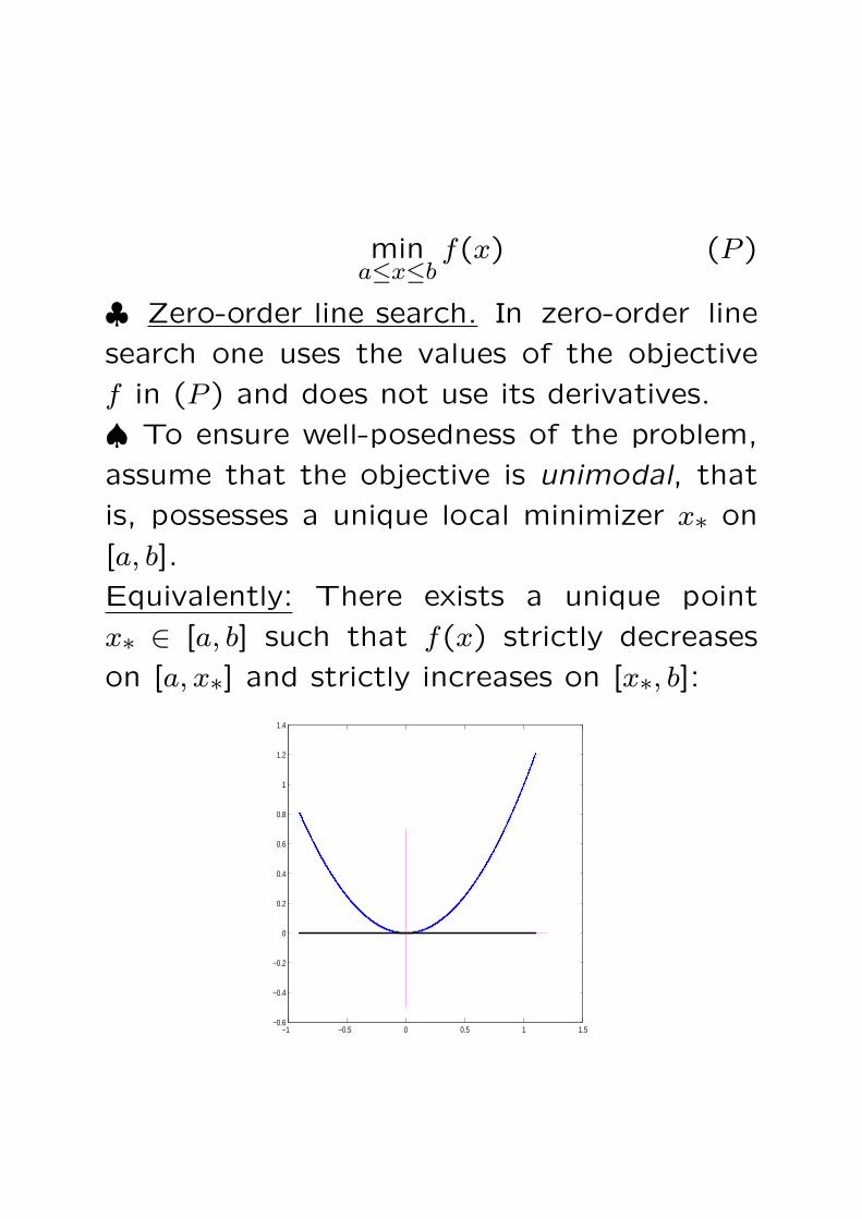
mina≤x≤b
f(x) (P )
♣ Zero-order line search. In zero-order line
search one uses the values of the objective
f in (P ) and does not use its derivatives.
♠ To ensure well-posedness of the problem,
assume that the objective is unimodal, that
is, possesses a unique local minimizer x∗ on
[a, b].
Equivalently: There exists a unique point
x∗ ∈ [a, b] such that f(x) strictly decreases
on [a, x∗] and strictly increases on [x∗, b]:
−1 −0.5 0 0.5 1 1.5−0.6
−0.4
−0.2
0
0.2
0.4
0.6
0.8
1
1.2
1.4

Main observation: Let f be unimodal on
[a, b], and assume we know f(x′), f(x′′) for
certain x′, x′′ with
a < x′ < x′′ < b.
♦If f(x′′) ≥ f(x′), then f(x) > f(x′′) for x >
x′′, so that the minimizer belongs to [a, x′′]:
−1 −0.5 0 0.5 1 1.5−0.6
−0.4
−0.2
0
0.2
0.4
0.6
0.8
1
1.2
1.4
♦Similarly, if f(x′′) < f(x′), then f(x > f(x′)when x < x′, so that the minimizer belongs
to [x′, b].♠ In both cases, two computations of f at x′,x′′ allow to reduce the initial “search domain”
with a smaller one ([a, x′′] or [x′, b]).

♣ Choosing x′, x′′ so that they split [a0, b0] =
[a, b] into three equal segments, computing
f(x′), f(x′′) and comparing them to each
other, we can build a new segment [a1, b1] ⊂[a0, b0] such that
♦the new segment is a localizer – it contains
the solution x∗♦the length of the new localizer is 2/3 of the
length of the initial localizer [a0, b0] = [a, b].
♠ On the new localizer, same as on the orig-
inal one, the objective is unimodal, and we
can iterate our construction.
♠ In N ≥ 1 steps (2N computations of f),
we shall reduce the size of localizer by factor
(2/3)N , that is, we get linearly converging,
in terms of the argument, algorithm with the
convergence ratio
q =√
2/3 = 0.8165...
Can we do better ? - YES!
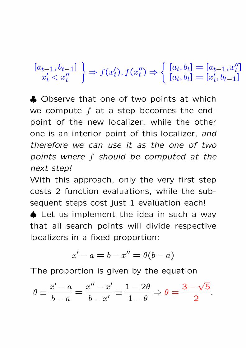
[at−1, bt−1]x′t < x′′t
⇒ f(x′t), f(x′′t ) ⇒
[at, bt] = [at−1, x′′t ][at, bt] = [x′t, bt−1]
♣ Observe that one of two points at which
we compute f at a step becomes the end-
point of the new localizer, while the other
one is an interior point of this localizer, and
therefore we can use it as the one of two
points where f should be computed at the
next step!
With this approach, only the very first step
costs 2 function evaluations, while the sub-
sequent steps cost just 1 evaluation each!
♠ Let us implement the idea in such a way
that all search points will divide respective
localizers in a fixed proportion:
x′ − a = b− x′′ = θ(b− a)
The proportion is given by the equation
θ ≡ x′ − a
b− a=
x′′ − x′
b− x′≡ 1− 2θ
1− θ⇒ θ =
3−√5
2.
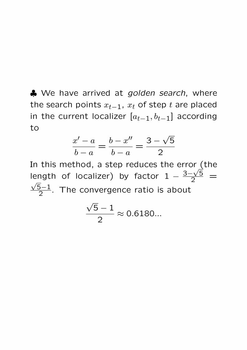
♣ We have arrived at golden search, where
the search points xt−1, xt of step t are placed
in the current localizer [at−1, bt−1] according
to
x′ − a
b− a=
b− x′′
b− a=
3−√5
2
In this method, a step reduces the error (the
length of localizer) by factor 1 − 3−√52 =√
5−12 . The convergence ratio is about
√5− 1
2≈ 0.6180...

minxf(x) : a ≤ x ≤ b ,
♣ First order line search: Bisection. Assume
that f is differentiable on (a, b) and strictly
unimodal, that is, it is unimodal, x∗ ∈ (a, b)
and f ′(x) < 0 for a < x < x∗, f ′(x) > 0 for
x∗ < x < b.
Let both f and f ′ be available. In this case
the method of choice in Bisection.
♠ Main observation: Given x1 ∈ [a, b] ≡[a0, b0], let us compute f ′(x1).
♦If f ′(x1) > 0, then, from strict unimodal-
ity, f(x) > f(x1) to the right of x1, thus, x∗belongs to [a, x1]:
−1 −0.5 0 0.5 1 1.5−0.6
−0.4
−0.2
0
0.2
0.4
0.6
0.8
1
1.2
1.4
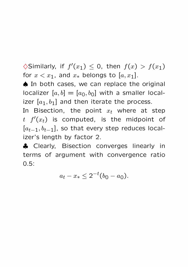
♦Similarly, if f ′(x1) ≤ 0, then f(x) > f(x1)
for x < x1, and x∗ belongs to [a, x1].
♠ In both cases, we can replace the original
localizer [a, b] = [a0, b0] with a smaller local-
izer [a1, b1] and then iterate the process.
In Bisection, the point xt where at step
t f ′(xt) is computed, is the midpoint of
[at−1, bt−1], so that every step reduces local-
izer’s length by factor 2.
♣ Clearly, Bisection converges linearly in
terms of argument with convergence ratio
0.5:
at − x∗ ≤ 2−t(b0 − a0).

Inexact Line Search
♣ Many algorithms for multi-dimensional
minimization which use Line Search as a sub-
routine, in the following way:
♦given current iterate xt ∈ Rn, the algorithm
defines a search direction dt ∈ Rn which is a
direction of decrease of f :
dTt ∇f(xt) < 0.
Then Line Search is invoked to minimize the
one-dimensional function
φ(s) = f(xt + γdt)
over γ ≥ 0; the resulting γ = γt defines the
stepsize along the direction dt, so that the
new iterate of the outer algorithm is
xt+1 = xt + γtdt.
♠ In many situations of this type, there is
no necessity in exact minimization in γ; an
“essential” reduction in φ is sufficient.
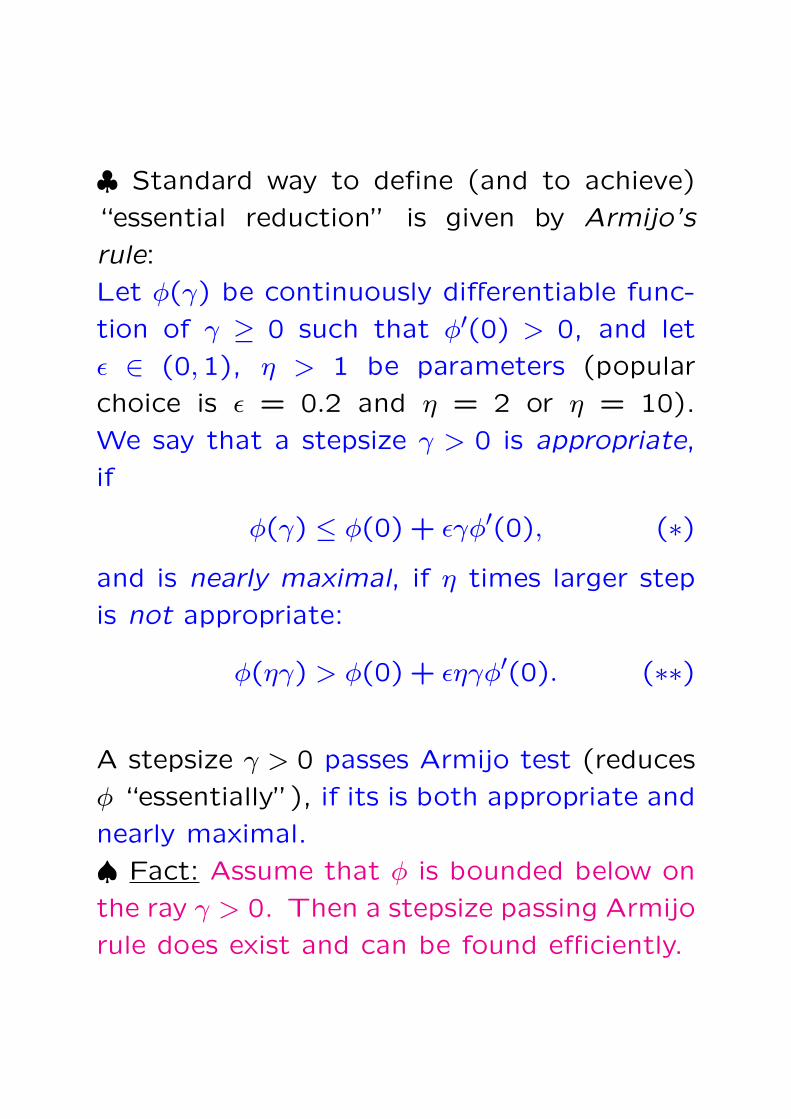
♣ Standard way to define (and to achieve)
“essential reduction” is given by Armijo’s
rule:
Let φ(γ) be continuously differentiable func-
tion of γ ≥ 0 such that φ′(0) > 0, and let
ε ∈ (0,1), η > 1 be parameters (popular
choice is ε = 0.2 and η = 2 or η = 10).
We say that a stepsize γ > 0 is appropriate,
if
φ(γ) ≤ φ(0) + εγφ′(0), (∗)and is nearly maximal, if η times larger step
is not appropriate:
φ(ηγ) > φ(0) + εηγφ′(0). (∗∗)
A stepsize γ > 0 passes Armijo test (reduces
φ “essentially”), if its is both appropriate and
nearly maximal.
♠ Fact: Assume that φ is bounded below on
the ray γ > 0. Then a stepsize passing Armijo
rule does exist and can be found efficiently.
♣ Armijo-acceptable step γ > 0:
φ(γ) ≤ φ(0) + εγφ′(0) (∗)φ(ηγ) > φ(0) + εηγφ′(0) (∗∗)
♣ Algorithm for finding Armijo-acceptable step:
Start: Choose γ0 > 0 and check whether it
passes (*). If YES, go to Branch A, other-
wise go to Branch B.
Branch A: γ0 satisfies (∗). Testing subse-
quently the values ηγ0, η2γ0, η3γ0,... of γ,
stop when the current value for the first time
violates (∗); the preceding value of γ passes
the Armijo test.
Branch B: γ0 does not satisfy (∗). Test-
ing subsequently the values η−1γ0, η−2γ0,
η−3γ0,... of γ, stop when the current value
for the first time satisfies (∗); this value of γ
passes the Armijo test.
♣ Validation of the algorithm: It is clear thatif the algorithm terminates, then the resultindeed passes the Armijo test. Thus, all weneed to verify is that the algorithm eventuallyterminates.♦Branch A clearly is finite: here we test theinequality
φ(γ) > φ(0) + εγφ′(0)
along the sequence γi = ηiγ0 → ∞, and ter-minate when this inequality is satisfied forthe first time. Since φ′(0) < 0 and φ is belowbounded, this indeed will eventually happen.♦Branch B clearly is finite: here we test theinequality
φ(γ) ≤ φ(0) + εγφ′(0) (∗)along a sequence γi = η−iγ0 → +0 of valuesof γ and terminate when this inequality issatisfied for the first time. Since ε ∈ (0,1)and φ′(0) < 0, this inequality is satisfied forall small enough positive values of γ, since
φ(γ) = φ(0) + γ[φ′(0) + R(γ)︸ ︷︷ ︸
→0,γ→+0
].
For large i, γi definitely will be “small enough”,thus, Branch B is finite.

Methods for Unconstrained Minimization
♣ Unconstrained minimization problem is
f∗ = minx
f(x),
where f well-defined and continuously differ-
entiable on the entire Rn.
Note: Most of the constructions to be pre-
sented can be straightforwardly extended
onto “essentially unconstrained case” where
f is continuously differentiable on an open
domain D in Rn and is such that the level
sets x ∈ U : f(x) ≤ a are closed.
f∗ = minx
f(x) (P )
Gradient Descent
♣ Gradient Descent is the simplest first ordermethod for unconstrained minimization.The idea: Let x be a current iterate which isnot a critical point of f : f ′(x) 6= 0. We have
f(x + th) = f(x) + thTf ′(x) + t‖h‖2Rx(th)[Rx(s) → 0 as s → 0]
Since f ′(x) 6= 0, the unit antigradient direc-tion g = −f ′(x)/‖f ′(x)‖2 is a direction of de-crease of f :
d
dt
∣∣∣t=0
f(x + tg) = gTf ′(x) = −‖f ′(x)‖2
so that shift x 7→ x + tg along the direction glocally decreases f “at the rate” ‖f ′(x)‖2.♠ Note: As far as local rate of decrease isconcerned, g is the best possible direction ofdecrease: for any other unit direction h, wehave
d
dt
∣∣∣t=0
f(x + th) = hTf ′(x) > −‖f ′(x)‖2.

♣ In generic Gradient Descent, we update
the current iterate x by a step from x in the
antigradient direction which reduces the ob-
jective:
xt = xt−1 − γtf′(xt−1),
where γt are positive stepsizes such that
f ′(xt−1) 6= 0 ⇒ f(xt) < f(xt−1).
♠ Standard implementations:
♦Steepest GD:
γt = argminγ≥0
f(xt−1 − γf ′(xt−1))
(slight idealization, except for the case of
quadratic f)
♦Armijo GD: γt > 0 is such that
f(xt−1 − γtf′(xt−1) ≤ f(xt−1)− εγt‖f ′(xt−1)‖22
f(xt−1 − ηγtf′(xt−1) > f(xt−1)− εηγt‖f ′(xt−1)‖22
(implementable, provided that f ′(xt−1) 6= 0
and f(xt−1 − γf ′(xt−1)) is below bounded
when γ ≥ 0)

Note: By construction, GD is unable to leave
a critical point:
f ′(xt−1) = 0 ⇒ xt = xt−1.
♣ Global Convergence Theorem: Assume that
the level set of f corresponding to the start-
ing point x0:
G = x : f(x) ≤ f(x0)is compact, and f is continuously differen-
tiable in a neighbourhood of G. Then for
both SGD and AGD:
♦the trajectory x0, x1, ... of the method, started
at x0, is well-defined and never leaves G (and
thus is bounded);
♦the method is monotone:
f(x0) ≥ f(x1) ≥ ...
and inequalities are strict, unless method
reaches a critical point xt, so that xt =
xt+1 = xt+2 = ...
♦Every limiting point of the trajectory is a
critical point of f .
Sketch of the proof: 10. If f ′(x0) = 0, the
method never leaves x0, and the statements
are evident. Now assume that f ′(x0) 6= 0.
Then the function φ0(γ) = f(x0− γf ′(x0)) is
below bounded, and the set γ ≥ 0 : φ0(γ) ≤φ0(0) is compact along with G, so that
φ0(γ) achieves its minimum on the ray γ ≥ 0,
and φ′0(0) < 0. It follows that the first step
of GD is well-defined and f(x1) < f(x0). The
set x : f(x) ≤ f(x1) is a closed subset of G
and thus is compact, and we can repeat our
reasoning with x1 in the role of x0, etc. We
conclude that the trajectory is well-defined,
never leaves G and the objective is strictly
decreased, unless a critical point is reached.
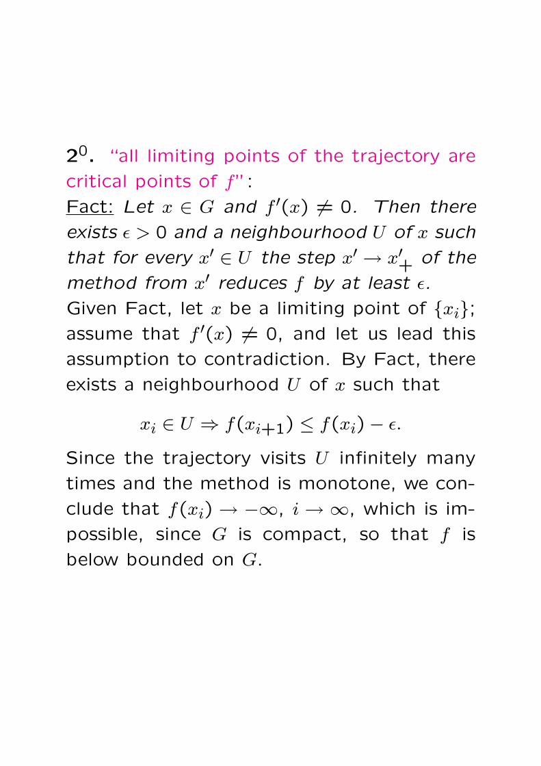
20. “all limiting points of the trajectory are
critical points of f”:
Fact: Let x ∈ G and f ′(x) 6= 0. Then there
exists ε > 0 and a neighbourhood U of x such
that for every x′ ∈ U the step x′ → x′+ of the
method from x′ reduces f by at least ε.
Given Fact, let x be a limiting point of xi;assume that f ′(x) 6= 0, and let us lead this
assumption to contradiction. By Fact, there
exists a neighbourhood U of x such that
xi ∈ U ⇒ f(xi+1) ≤ f(xi)− ε.
Since the trajectory visits U infinitely many
times and the method is monotone, we con-
clude that f(xi) → −∞, i → ∞, which is im-
possible, since G is compact, so that f is
below bounded on G.

Limiting points of Gradient Descent
♣ Under assumptions of Global Convergence
Theorem, limiting points of GD exist, and all
of them are critical points of f . What kind
of limiting points could they be?
♦A nondegenerate maximizer of f cannot be
a limiting point of GD, unless the method is
started at this maximizer.
♦A saddle point of f is “highly unlikely”
candidate to the role of a limiting point.
Practical experience says that limiting points
are local minimizers of f .
♦A nondegenerate global minimizer x∗ of f ,
if any, as an “attraction point” of GD: when
starting close enough to this minimizer, the
method converges to x∗.

Rates of convergence
♣ In general, we cannot guarantee more thanconvergence to the set of critical points of f .A natural error measure associated with thisset is
δ2(x) = ‖f ′(x)‖22.
♠ Definition: Let U be an open subset of Rn,L ≥ 0 and f be a function defined on U . Wesay that f is C1,1(L) on U , if f is continu-ously differentiable in U with locally Lipschitzcontinuous, with constant L, gradient:
[x, y] ∈ U ⇒ ‖f ′(x)− f ′(y)‖2 ≤ L‖x− y‖2.
We say that f is C1,1(L) on a set Q ⊂ Rn, ifthere exists an open set U ⊃ Q such that f
is C1,1(L) on U .Note: Assume that f is twice continuouslydifferentiable on U . Then f is C1,1(L) onU iff the norm of the Hessian of f does notexceed L:
∀(x ∈ U, d ∈ Rn) : |dTf ′′(x)d| ≤ L‖d‖22.
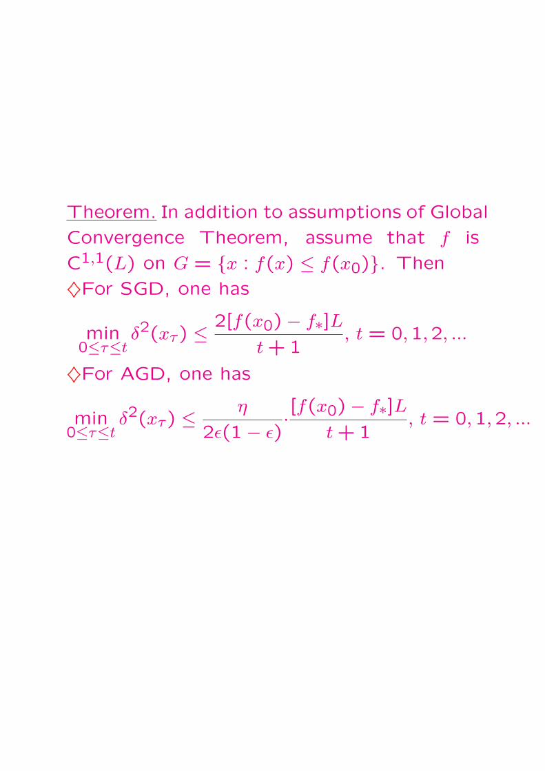
Theorem. In addition to assumptions of Global
Convergence Theorem, assume that f is
C1,1(L) on G = x : f(x) ≤ f(x0). Then
♦For SGD, one has
min0≤τ≤t
δ2(xτ) ≤ 2[f(x0)− f∗]Lt + 1
, t = 0,1,2, ...
♦For AGD, one has
min0≤τ≤t
δ2(xτ) ≤ η
2ε(1− ε)·[f(x0)− f∗]L
t + 1, t = 0,1,2, ...
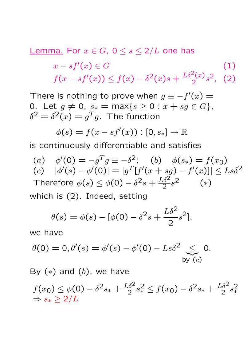
Lemma. For x ∈ G, 0 ≤ s ≤ 2/L one has
x− sf ′(x) ∈ G (1)
f(x− sf ′(x)) ≤ f(x)− δ2(x)s + Lδ2(x)2 s2, (2)
There is nothing to prove when g ≡ −f ′(x) =0. Let g 6= 0, s∗ = maxs ≥ 0 : x + sg ∈ G,δ2 = δ2(x) = gTg. The function
φ(s) = f(x− sf ′(x)) : [0, s∗] → Ris continuously differentiable and satisfies
(a) φ′(0) = −gTg ≡ −δ2; (b) φ(s∗) = f(x0)(c) |φ′(s)− φ′(0)| = |gT [f ′(x + sg)− f ′(x)]| ≤ Lsδ2
Therefore φ(s) ≤ φ(0)− δ2s + Lδ2
2 s2 (∗)which is (2). Indeed, setting
θ(s) = φ(s)− [φ(0)− δ2s +Lδ2
2s2],
we have
θ(0) = 0, θ′(s) = φ′(s)− φ′(0)− Lsδ2 ≤︸︷︷︸by (c)
0.
By (∗) and (b), we have
f(x0) ≤ φ(0)− δ2s∗ + Lδ2
2 s2∗ ≤ f(x0)− δ2s∗ + Lδ2
2 s2∗⇒ s∗ ≥ 2/L

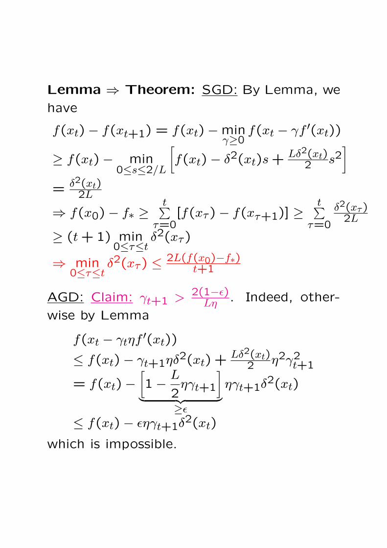
Lemma ⇒ Theorem: SGD: By Lemma, we
have
f(xt)− f(xt+1) = f(xt)−minγ≥0
f(xt − γf ′(xt))
≥ f(xt)− min0≤s≤2/L
[f(xt)− δ2(xt)s + Lδ2(xt)
2 s2]
= δ2(xt)2L
⇒ f(x0)− f∗ ≥t∑
τ=0[f(xτ)− f(xτ+1)] ≥
t∑τ=0
δ2(xτ)2L
≥ (t + 1) min0≤τ≤t
δ2(xτ)
⇒ min0≤τ≤t
δ2(xτ) ≤ 2L(f(x0)−f∗)t+1
AGD: Claim: γt+1 > 2(1−ε)Lη . Indeed, other-
wise by Lemma
f(xt − γtηf ′(xt))
≤ f(xt)− γt+1ηδ2(xt) + Lδ2(xt)2 η2γ2
t+1
= f(xt)−[1− L
2ηγt+1
]
︸ ︷︷ ︸≥ε
ηγt+1δ2(xt)
≤ f(xt)− εηγt+1δ2(xt)
which is impossible.
We have seen that γt+1 > 2(1−ε)Lη . By Armijo
rule,
f(xt)−f(xt+1) ≥ εγt+1δ2(xt) ≥2ε(1− ε)
Lηδ2(xt);
the rest of the proof is as for SGD.
♣ Convex case. In addition to assumptions of
Global Convergence Theorem, assume that f
is convex.
♠ All critical points of a convex function are
its global minimizers
⇒ In Convex case, SGD and AGD converge
to the set of global minimizers of f : f(xt) →f∗ as t → ∞, and all limiting points of the
trajectory are global minimizers of f .
♠ In Convex C1,1(L) case, one can quantify
the global rate of convergence in terms of
the residual f(xt)− f∗:Theorem. Assume that the set G = x :
f(x) ≤ f(x0) is convex compact, f is convex
on G and C1,1(L) on this set. Consider AGD,
and let ε ≥ 0.5. Then the trajectory of the
method converges to a global minimizer x∗of f , and
f(xt)− f∗ ≤ ηL‖x0 − x∗‖224(1− ε)t
, t = 1,2, ...

♣ Definition: Let M be a convex set in Rn
and 0 < ` ≤ L < ∞. A function f is calledstrongly convex, with parameters `, L, on M ,if♦f is C1,1(L) on M♦for x, y ∈ M , one has
[x− y]T [f ′(x)− f ′(y)] ≥ `‖x− y‖22. (∗)The ratio Qf = L/` is called condition numberof f .♠ Comment: If f is C1,1(L) on a convex setM , then
x, y ∈ M ⇒ |f(y)−[f(x)+(y−x)Tf ′(x)]| ≤ L
2‖x−y‖22.
If f satisfies (∗) on a convex set M , then
∀x, y ∈ M : f(y) ≥ f(x)+(y−x)Tf ′(x)+ `
2‖y−x‖22.
In particular, f is convex on M .⇒ A strongly convex, with parameters `, L,function f on a convex set M satisfies therelation
∀x, y ∈ M : f(x) + (y − x)Tf ′(x) + `2‖y − x‖22
≤ f(y) ≤ f(x) + (y − x)Tf ′(x) + L2‖y − x‖22
Note: Assume that f is twice continuously
differentiable in a neighbourhood of a convex
set M . Then f is (`, L)-strongly convex on
M iff for all x ∈ M and all d ∈ Rn one has
`‖d‖22 ≤ dTf ′′(x)d ≤ L‖d‖22m
λmin(f′′(x)) ≥ `, λmax(f ′′(x)) ≤ L.
In particular,
♠ A quadratic function
f(x) =1
2xTAx− bTx + c
with positive definite symmetric matrix A
is strongly convex with the parameters ` =
λmin(A), L = λmax(A) on the entire space.

♣ GD in strongly convex case.
Theorem. In the strongly convex case, AGD
exhibits linear global rate of convergence.
Specifically, let the set G = x : f(x) ≤f(x0) be closed and convex and f be strongly
convex, with parameters `, L, on Q. Then
x ♦G is compact, and the global minimizer
x∗ of f exists and is unique;
♦AGD with ε ≥ 1/2 converges linearly to x∗:
‖xt − x∗‖2 ≤ θt‖x0 − x∗‖2
θ =
√Qf−(2−ε−1)(1−ε)η−1
Qf+(ε−1−1)η−1 = 1−O(Q−1f ).
Besides this,
f(xt)− f∗ ≤ θ2tQf [f(x0)− f∗].
♣ SGD in Strongly convex quadratic case.
Assume that f(x) = 12xTAx − bTx + c is a
strongly convex quadratic function: A =
AT Â 0. In this case, SGD becomes imple-
mentable and is given by the recurrence
gt = f ′(xt) = Axt − b
γt+1 =gTt gt
gTt Agt
xt+1 = xt − γt+1gt
and guarantees that
f(xt+1)− f∗︸ ︷︷ ︸Et+1
≤[1− (gT
t gt)2
[gTt Agt][gT
t A−1gt]
]Et ≤
(Qf−1Qf+1
)2Et
whence
f(xt)−f∗ ≤(
Qf − 1
Qf + 1
)2t
[f(x0)−f∗], t = 1,2, ...

Note: If we know that SGD converges to
a nondegenerate local minimizer x∗ of f ,
then, under mild regularity assumptions, the
asymptotical behaviour of the method will be
as if f were the strongly convex quadratic
form
f(x) = const +1
2(x− x∗)Tf ′′(x∗)(x− x∗).


0 100 200 300 400 500 600 700 800 900 100010
−4
10−3
10−2
10−1
100
Plot of f(xt)−f∗
(f(x0)−f∗)(
Qf−1
Qf+1
)2t
SGD as applied to quadratic form with Qf = 1000
♦f(x0) = 2069.4, f(x999) = 0.0232
♣ Summary on Gradient Descent:
♦Under mild regularity and boundedness as-
sumptions, both SGD and AGD converge the
set of critical points of the objective.
In the case of C1,1(L)-smooth objective, the
methods exhibit non-asymptotical O(1/t)-
rate of convergence in terms of the error
measure δ2(x) = ‖f ′(x)‖22.♦Under the same regularity assumptions, in
Convex case the methods converge to the set
of glomal minimizers of the objective.
In convex C1,1(L)-case, AGD exhibits non-
asymptotical O(1/t) rate of convergence in
terms of the residual in the objective f(x)−f∗♦In Strongly convex case, AGD exhibits non-
asymptotical linear convergence in both the
residual in terms of the objective f(x) − f∗and the distance in the argument ‖x− x∗‖2.The convergence ratio is 1−O(1/Qf), where
Qf is the all condition number of the objec-
tive. In other words, to get extra accuracy
digit, it takes O(Qf) steps.

♣ Good news on GD:
♠ Simplicity
♠ Reasonable global convergence properties
under mild assumptions on the function to
be minimized.

♣ Drawbacks of GD:
♠ “Frame-dependence”: The method is not
affine invariant!
♦You are solving the problem minx
f(x) by
GD, starting with x0 = 0, Your first search
point will be
x1 = −γ1f ′(0).
♦I solve the same problem, but in new vari-
ables y: x = Ay. My problem is miny
g(y),
g(y) = f(Ax), and start with y0 = 0. My
first search point will be
y1 = −γ1g′(0) = −γ1ATf ′(0).
In x-variables, my search point will be
x1 = Ay1 = −γ1AATf ′(0)
If AAT is not proportional to the unit matrix,
my search point will, in general, be different
from yours!

♠ “Frame-dependence” is common draw-
back of nearly all first order optimization
methods, and this is what makes their rate of
convergence, even under the most favourable
case of strongly convex objective, sensitive
to the condition number of the problem. GD
is “hyper-sensitive” to the condition number:
When minimizing strongly convex function f ,
the convergence ratio of GD is 1−O(1/Qf),
while for better methods it is 1−O(1/Q1/2f ).
The Newton Method
♣ Consider unconstrained problem
minx
f(x)
with twice continuously differentiable objec-tive. Assuming second order informationavailable, we approximate f around a currentiterate x by the second order Taylor expan-sion:
f(y) ≈ f(x)+(y−x)Tf ′(x)+(y − x)Tf ′′(x)(y − x)
2In the Newton method, the new iterate is theminimizer of this quadratic approximation. Ifexists, the minimizer is given by
∇y[f(x) + (y − x)Tf ′(x) + (y−x)T f ′′(x)(y−x)2 ] = 0
⇔ f ′′(x)(y − x) = −f ′(x)⇔ y = x− [f ′′(x)]−1f ′(x)
We have arrived at the Basic Newton method
xt+1 = xt − [f ′′(xt)]−1f ′(xt)
(step t is undefined when the matrix f ′′(xt)is singular).

xt+1 = xt − [f ′′(xt)]−1f ′(xt)
♠ Alternative motivation: We seek for a so-
lution to the Fermat equation
f ′(x) = 0;
given current approximate xt to the solution,
we linearize the left hand side around xt, thus
arriving at the linearized Fermat equation
f ′(xt) + f ′′(xt)[x− xt] = 0
and take the solution to this equation, that
is, xt − [f ′′(xt)]−1f ′(xt), as our new iterate.
xt+1 = xt − [f ′′(xt)]−1f ′(xt) (Nwt)
Theorem on Local Quadratic Convergence: Let
x∗ be a nondegenerate local minimizer of
f , so that f ′′(x∗) Â 0, and let f be three
times continuously differentiable in a neigh-
bourhood of x∗. Then the recurrence (Nwt),
started close enough to x∗, is well-defined
and converges to x∗ quadratically.
Proof: 10. Let U be a ball centered at x∗where the third derivatives of f are bounded.
For y ∈ U one has
‖∇f(y)−∇2f(y)(x∗ − y)‖2≡ ‖∇f(x∗)−∇f(y)−∇2f(y)(x∗ − y)‖2≤ β1‖y − x∗‖22
(1)
20. Since f ′′(x) is continuous at x = x∗ and
f ′′(x∗) is nonsingular, there exists a ball U ′ ⊂U centered at x∗ such that
y ∈ U ′ ⇒ ‖[f ′′(y)]−1‖ ≤ β2. (2)

Situation: There exists a r > 0 and positive
constants β1, β2 such that
‖y − x∗‖ < r ⇒(a) ‖∇f(y)−∇2f(y)(x∗ − y)‖2 ≤ β1‖y − x∗‖22(b) ‖[f ′′(y)]−1‖ ≤ β2
30. Let an iterate xt of the method be close
to x∗:
xt ∈ V = x : ‖x− x∗‖@ ≤ ρ ≡ min[1
2β1β2, r].
We have
‖xt+1 − x∗‖ = ‖xt − x∗ − [f ′′(xt)]−1f ′(xt)‖2= ‖
[[f ′′(xt)]−1[f ′′(xt)(xt − x∗)− f ′(xt)]
]‖2
≤ β1β2‖xt − x∗‖22 ≤ 0.5‖xt − x∗‖2We conclude that the method remains well-
defined after step t, and converges to x∗quadratically.
♣ A remarkable property of Newton method
is affine invariance (”frame independence”):
Let x = Ay + b be invertible affine change of
variables. Then
f(x) ⇔ g(y) = f(Ay + b)x = Ay + b ⇔ y
y+ = y − [g′′(y)]−1g′(y)= y − [ATf ′′(x)A]−1[ATf ′(x)]= y −A−1[f ′′(x)]−1f ′(x)⇒ Ay+ + b = [Ay + b]−[f ′′(x)]−1f ′(x)= x− [f ′′(x)]−1f ′(x)
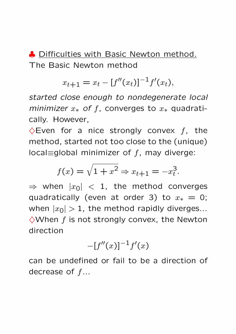
♣ Difficulties with Basic Newton method.
The Basic Newton method
xt+1 = xt − [f ′′(xt)]−1f ′(xt),
started close enough to nondegenerate local
minimizer x∗ of f , converges to x∗ quadrati-
cally. However,
♦Even for a nice strongly convex f , the
method, started not too close to the (unique)
local≡global minimizer of f , may diverge:
f(x) =√
1 + x2 ⇒ xt+1 = −x3t .
⇒ when |x0| < 1, the method converges
quadratically (even at order 3) to x∗ = 0;
when |x0| > 1, the method rapidly diverges...
♦When f is not strongly convex, the Newton
direction
−[f ′′(x)]−1f ′(x)
can be undefined or fail to be a direction of
decrease of f ...

♣ As a result of these drawbacks, one needs
to modify the Basic Newton method in order
to ensure global convergence. Modifications
include:
♦Incorporating line search
♦Correcting Newton direction when it is un-
defined or is not a direction of decrease of f .
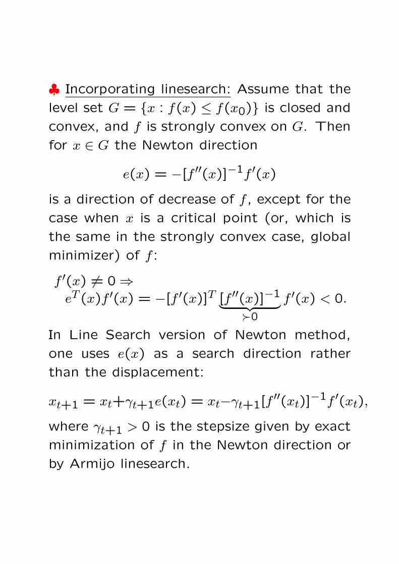
♣ Incorporating linesearch: Assume that the
level set G = x : f(x) ≤ f(x0) is closed and
convex, and f is strongly convex on G. Then
for x ∈ G the Newton direction
e(x) = −[f ′′(x)]−1f ′(x)
is a direction of decrease of f , except for the
case when x is a critical point (or, which is
the same in the strongly convex case, global
minimizer) of f :
f ′(x) 6= 0 ⇒eT (x)f ′(x) = −[f ′(x)]T [f ′′(x)]−1
︸ ︷︷ ︸Â0
f ′(x) < 0.
In Line Search version of Newton method,
one uses e(x) as a search direction rather
than the displacement:
xt+1 = xt+γt+1e(xt) = xt−γt+1[f′′(xt)]
−1f ′(xt),
where γt+1 > 0 is the stepsize given by exact
minimization of f in the Newton direction or
by Armijo linesearch.

Theorem: Let the Level set G = x : f(x) ≤f(x0) be convex and compact, and f be
strongly convex on G. Then Newton method
with the Steepest Descent or with the Armijo
linesearch converges to the unique global
minimizer of f .
With proper implementation of the line-
search, convergence is quadratic.

♣ Newton method: Summary
♦Good news: Quadratic asymptotical con-
vergence, provided we manage to bring the
trajectory close to a nondegenerate local
minimizer
♦Bad news:
— relatively high computational cost, com-
ing from the necessity to compute and to
invert the Hessian matrix
— necessity to “cure” the method in the
non-strongly-convex case, where the Newton
direction can be undefined or fail to be a di-
rection of decrease...
Modifications of the Newton method
♣ Modifications of the Newton method are
aimed at overcoming its shortcomings (diffi-
culties with nonconvex objectives, relatively
high computational cost) while preserving its
major advantage – rapid asymptotical con-
vergence. There are three major groups of
modifications:
♦Modified Newton methods based on second-
order information
♦Modifications based on first order informa-
tion:
— conjugate gradient methods
— quasi-Newton methods
♠ All modifications of Newton method ex-
ploit a natural Variable Metric idea.
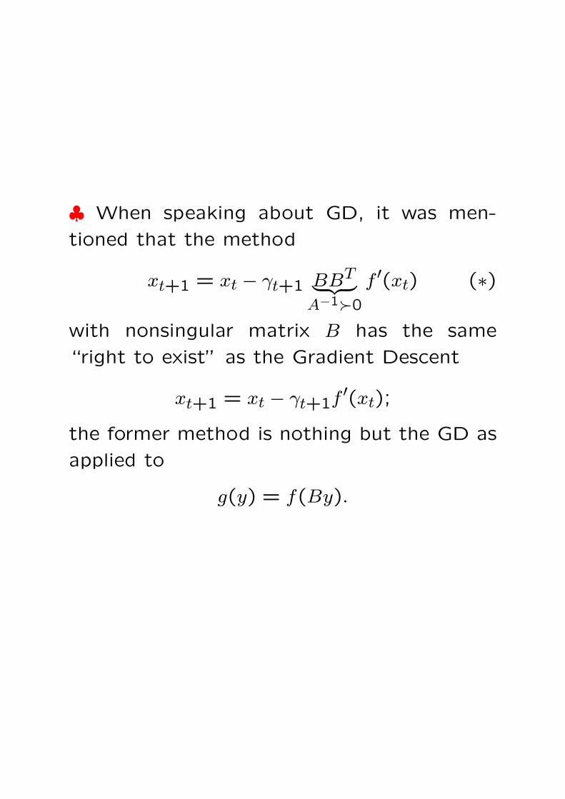
♣ When speaking about GD, it was men-
tioned that the method
xt+1 = xt − γt+1 BBT︸ ︷︷ ︸A−1Â0
f ′(xt) (∗)
with nonsingular matrix B has the same
“right to exist” as the Gradient Descent
xt+1 = xt − γt+1f ′(xt);
the former method is nothing but the GD as
applied to
g(y) = f(By).
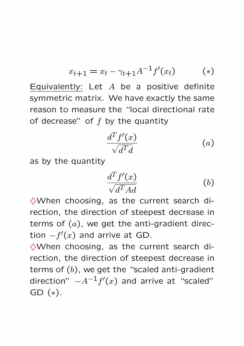
xt+1 = xt − γt+1A−1f ′(xt) (∗)Equivalently: Let A be a positive definite
symmetric matrix. We have exactly the same
reason to measure the “local directional rate
of decrease” of f by the quantity
dTf ′(x)√dTd
(a)
as by the quantity
dTf ′(x)√dTAd
(b)
♦When choosing, as the current search di-
rection, the direction of steepest decrease in
terms of (a), we get the anti-gradient direc-
tion −f ′(x) and arrive at GD.
♦When choosing, as the current search di-
rection, the direction of steepest decrease in
terms of (b), we get the “scaled anti-gradient
direction” −A−1f ′(x) and arrive at “scaled”
GD (∗).

♣ We have motivated the scaled GD
xt+1 = xt − γt+1A−1f ′(xt) (∗)Why not to take one step ahead by consider
a generic Variable Metric algorithm
xt+1 = xt − γt+1A−1t+1f ′(xt) (VM)
with “scaling matrix” At+1 Â 0 varying from
step to step?
♠ Note: When At+1 ≡ I, (VM) becomes the
generic Gradient Descent;
When f is strongly convex and At+1 =
f ′′(xt), (VM) becomes the generic Newton
method...
♠ Note: When xt is not a critical point of f ,
the search direction dt+1 = −A−1t+1f ′(xt) is a
direction of decrease of f :
dTt+1f ′(xt) = −[f ′(xt)]
TA−1t+1f ′(xt) < 0.
Thus, we have no conceptual difficulties with
monotone linesearch versions of (VM)...

xt+1 = xt − γt+1A−1t+1f ′(xt) (VM)
♣ It turns out that Variable Metric methods
possess good global convergence properties:
Theorem: Let the level set G = x : f(x) ≤f(x0) be closed and bounded, and let f be
twice continuously differentiable in a neigh-
bourhood of G.
Assume, further, that the policy of updating
the matrices At ensures their uniform positive
definiteness and boundedness:
∃0 < ` ≤ L < ∞ : `I ¹ At ¹ LI ∀t.Then for both the Steepest Descent and the
Armijo versions of (VM) started at x0, the
trajectory is well-defined, belongs to G (and
thus is bounded), and f strictly decreases
along the trajectory unless a critical point of
f is reached. Moreover, all limiting points of
the trajectory are critical points of f .

♣ Implementation via Spectral Decomposition:
♦Given xt, compute Ht = f ′′(xt) and then
find spectral decomposition of Ht:
Ht = VtDiagλ1, ..., λnV Tt
♦Given once for ever chosen tolerance δ > 0,
set
λi = max[λi, δ]
and
At+1 = VtDiagλ1, ..., λnV Tt
Note: The construction ensures uniform pos-
itive definiteness and boundedness of Att,provided the level set G = x : f(x) ≤ f(x0)is compact and f is twice continuously dif-
ferentiable in a neighbourhood of G.
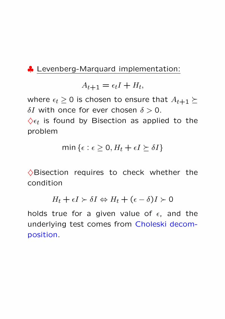
♣ Levenberg-Marquard implementation:
At+1 = εtI + Ht,
where εt ≥ 0 is chosen to ensure that At+1 ºδI with once for ever chosen δ > 0.
♦εt is found by Bisection as applied to the
problem
min ε : ε ≥ 0, Ht + εI º δI
♦Bisection requires to check whether the
condition
Ht + εI Â δI ⇔ Ht + (ε− δ)I Â 0
holds true for a given value of ε, and the
underlying test comes from Choleski decom-
position.

♣ Choleski Decomposition. By Linear Alge-bra, a symmetric matrix P is  0 iff
P = DDT (∗)with lower triangular nonsingular matrix D.When Choleski Decomposition (∗) exists, itcan be found by a simple algorithm as fol-lows:♦Representation (∗) means that
pij = didTj ,
where
di = (di1, di2, ..., dii,0,0,0,0, ...,0)dj = (dj1, dj2, ..., dji, ..., djj,0, ...,0)
are the rows of D.♦In particular, pi1 = d11di1, and we can setd11 =
√p11, di1 = pi1/d11, thus specifying
the first column of D.♦Further, p22 = d2
21 + d222, whence d22 =√
p22 − d221. After we know d22, we can find
all remaining entries in the second column ofD from the relations
pi2 = di1d21+di2d22 ⇒ di2 =pi2 − di1d21
d22, i > 2.
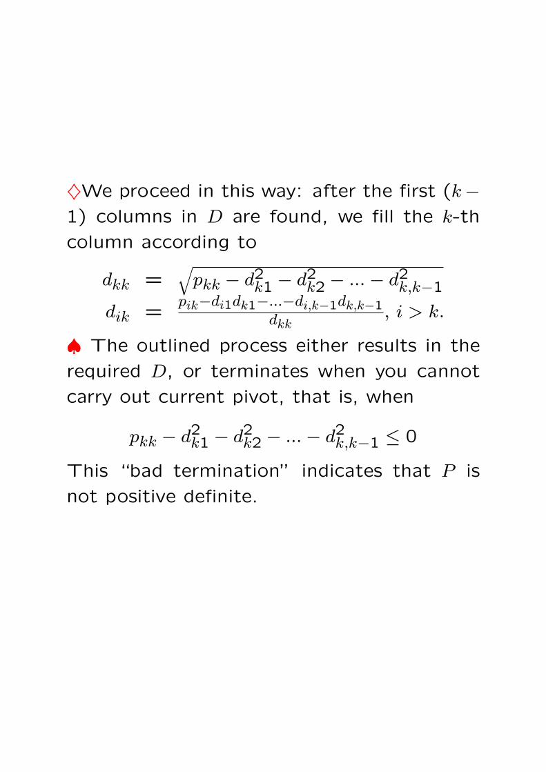
♦We proceed in this way: after the first (k−1) columns in D are found, we fill the k-th
column according to
dkk =√
pkk − d2k1 − d2
k2 − ...− d2k,k−1
dik =pik−di1dk1−...−di,k−1dk,k−1
dkk, i > k.
♠ The outlined process either results in the
required D, or terminates when you cannot
carry out current pivot, that is, when
pkk − d2k1 − d2
k2 − ...− d2k,k−1 ≤ 0
This “bad termination” indicates that P is
not positive definite.

The outlined Choleski Algorithm allows to
find the Choleski decomposition, if any, in
≈ n3
6 a.o. It is used routinely to solve linear
systems
Px = p (S)
with P Â 0. To solve the system, one first
computes the Choleski decomposition
P = DDT
and then solves (S) by two back-substitutions
b 7→ y : Dy = b, y 7→ x : DTx = y,
that is, by solving two triangular systems of
equations (which takes just O(n2) a.o.
Another application of the algorithm (e.g.,
in Levenberg-Marquardt method) is to check
positive definiteness of a symmetric matrix.
Note: The Levenberg-Marquardt method pro-
duces uniformly positive definite bounded se-
quence At, provided that the set G = x :
f(x) ≤ f(x0) is compact and f is twice con-
tinuously differentiable in a neighbourhood of
G.

♣ The “most practical” implementation of
Modified Newton Method is based on run-
ning the Choleski decomposition as applied
to Ht = f ′′(xt). When in course of this pro-
cess the current pivot (that is, specifying dkk)
becomes impossible or results in dkk < δ, one
increases the corresponding diagonal entry in
Ht until the condition dkk = δ is met.
With this approach, one finds a diagonal cor-
rection of Ht which makes the matrix “well
positive definite” and ensures uniform posi-
tive definiteness and boundedness of the re-
sulting sequence At, provided that the set
G = x : f(x) ≤ f(x0) is compact and f is
twice continuously differentiable in a neigh-
bourhood of G.
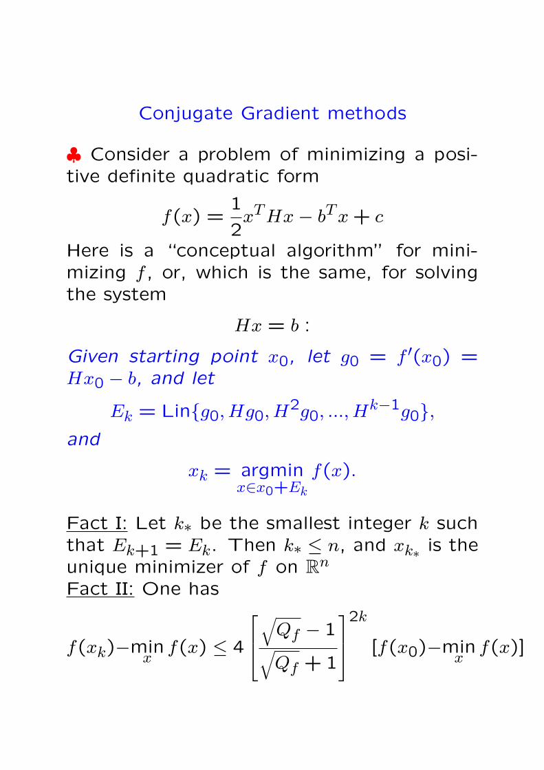
Conjugate Gradient methods
♣ Consider a problem of minimizing a posi-tive definite quadratic form
f(x) =1
2xTHx− bTx + c
Here is a “conceptual algorithm” for mini-mizing f , or, which is the same, for solvingthe system
Hx = b :
Given starting point x0, let g0 = f ′(x0) =Hx0 − b, and let
Ek = Ling0, Hg0, H2g0, ..., Hk−1g0,and
xk = argminx∈x0+Ek
f(x).
Fact I: Let k∗ be the smallest integer k suchthat Ek+1 = Ek. Then k∗ ≤ n, and xk∗ is theunique minimizer of f on Rn
Fact II: One has
f(xk)−minx
f(x) ≤ 4
√Qf − 1
√Qf + 1
2k
[f(x0)−minx
f(x)]
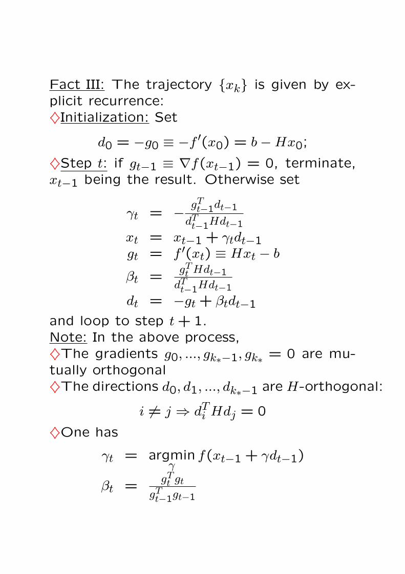
Fact III: The trajectory xk is given by ex-plicit recurrence:♦Initialization: Set
d0 = −g0 ≡ −f ′(x0) = b−Hx0;
♦Step t: if gt−1 ≡ ∇f(xt−1) = 0, terminate,xt−1 being the result. Otherwise set
γt = − gTt−1dt−1
dTt−1Hdt−1
xt = xt−1 + γtdt−1gt = f ′(xt) ≡ Hxt − b
βt =gTt Hdt−1
dTt−1Hdt−1
dt = −gt + βtdt−1
and loop to step t + 1.Note: In the above process,♦The gradients g0, ..., gk∗−1, gk∗ = 0 are mu-tually orthogonal♦The directions d0, d1, ..., dk∗−1 are H-orthogonal:
i 6= j ⇒ dTi Hdj = 0
♦One has
γt = argminγ
f(xt−1 + γdt−1)
βt =gTt gt
gTt−1gt−1
♣ Conjugate Gradient method as applied to
a strongly convex quadratic form f can be
viewed as an iterative algorithm for solving
the linear system
Hx = b.
As compared to “direct solvers”, like Choleski
Decomposition or Gauss elimination, the ad-
vantages of CG are:
♦Ability, in the case of exact arithmetic, to
find solution in at most n steps, with a single
matrix-vector multiplication and O(n) addi-
tional operations per step.
⇒ The cost of finding the solution is at most
O(n)L, where L is the arithmetic price of
matrix-vector multiplication.
Note: When H is sparse, L << n2, and the
price of the solution becomes much smaller
than the price O(n3) for the direct LA meth-
ods.
♦In principle, there is no necessity to assem-
ble H – all we need is the possibility to mul-
tiply by H

♦The non-asymptotic error bound
f(xk)−minx
f(x) ≤ 4
√Qf − 1
√Qf + 1
2k
[f(x0)−minx
f(x)]
indicates rate of convergence completely in-
dependent of the dimension and depending
only on the condition number of H.
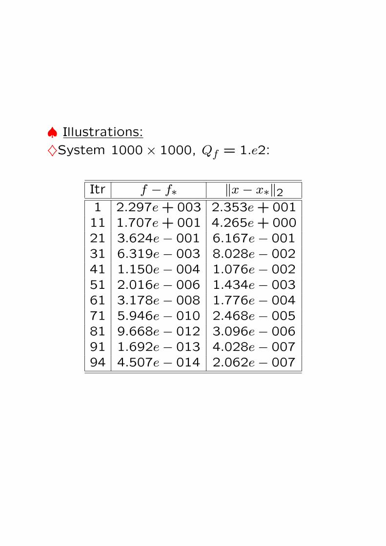
♠ Illustrations:
♦System 1000× 1000, Qf = 1.e2:
Itr f − f∗ ‖x− x∗‖21 2.297e + 003 2.353e + 00111 1.707e + 001 4.265e + 00021 3.624e− 001 6.167e− 00131 6.319e− 003 8.028e− 00241 1.150e− 004 1.076e− 00251 2.016e− 006 1.434e− 00361 3.178e− 008 1.776e− 00471 5.946e− 010 2.468e− 00581 9.668e− 012 3.096e− 00691 1.692e− 013 4.028e− 00794 4.507e− 014 2.062e− 007
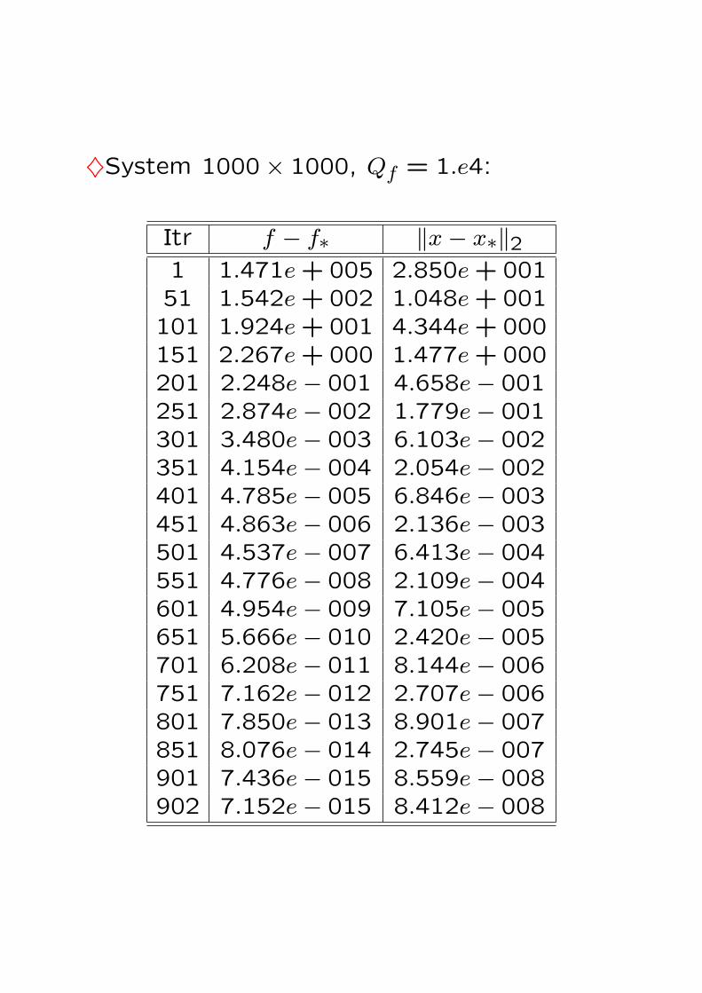
♦System 1000× 1000, Qf = 1.e4:
Itr f − f∗ ‖x− x∗‖21 1.471e + 005 2.850e + 00151 1.542e + 002 1.048e + 001101 1.924e + 001 4.344e + 000151 2.267e + 000 1.477e + 000201 2.248e− 001 4.658e− 001251 2.874e− 002 1.779e− 001301 3.480e− 003 6.103e− 002351 4.154e− 004 2.054e− 002401 4.785e− 005 6.846e− 003451 4.863e− 006 2.136e− 003501 4.537e− 007 6.413e− 004551 4.776e− 008 2.109e− 004601 4.954e− 009 7.105e− 005651 5.666e− 010 2.420e− 005701 6.208e− 011 8.144e− 006751 7.162e− 012 2.707e− 006801 7.850e− 013 8.901e− 007851 8.076e− 014 2.745e− 007901 7.436e− 015 8.559e− 008902 7.152e− 015 8.412e− 008
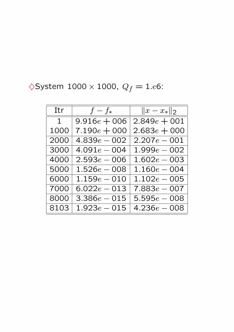
♦System 1000× 1000, Qf = 1.e6:
Itr f − f∗ ‖x− x∗‖21 9.916e + 006 2.849e + 001
1000 7.190e + 000 2.683e + 0002000 4.839e− 002 2.207e− 0013000 4.091e− 004 1.999e− 0024000 2.593e− 006 1.602e− 0035000 1.526e− 008 1.160e− 0046000 1.159e− 010 1.102e− 0057000 6.022e− 013 7.883e− 0078000 3.386e− 015 5.595e− 0088103 1.923e− 015 4.236e− 008
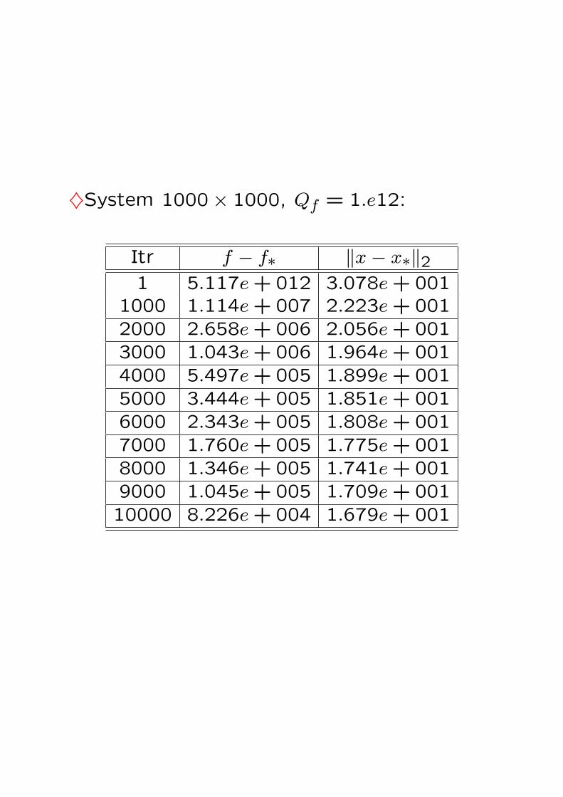
♦System 1000× 1000, Qf = 1.e12:
Itr f − f∗ ‖x− x∗‖21 5.117e + 012 3.078e + 001
1000 1.114e + 007 2.223e + 0012000 2.658e + 006 2.056e + 0013000 1.043e + 006 1.964e + 0014000 5.497e + 005 1.899e + 0015000 3.444e + 005 1.851e + 0016000 2.343e + 005 1.808e + 0017000 1.760e + 005 1.775e + 0018000 1.346e + 005 1.741e + 0019000 1.045e + 005 1.709e + 00110000 8.226e + 004 1.679e + 001

♣ Non-Quadratic Extensions: CG in the form
d0 = −g0 = −f ′(x0)γt = argmin
γf(xt−1 + γdt−1)
xt = xt−1 + γtdt−1gt = f ′(xt)
βt =gTt gt
gTt−1gt−1
dt = −gt + βtdt−1
can be applied to whatever function f , notnecessarily quadratic one (Fletcher-Reevs CG),and similarly for another equivalent in thequadratic case form:
d0 = −g0 = −f ′(x0)γt = argmin
γf(xt−1 + γdt−1)
xt = xt−1 + γtdt−1gt = f ′(xt)
βt =(gt−gt−1)
T gt
gTt−1gt−1
dt = −gt + βtdt−1
(Polak-Ribiere CG).♠ Being equivalent in the quadratic case,these (and other) forms of CG become dif-ferent in the non-quadratic case!
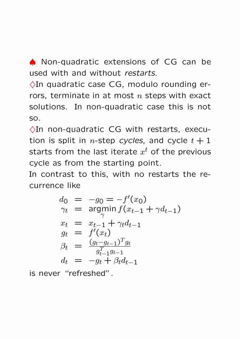
♠ Non-quadratic extensions of CG can be
used with and without restarts.
♦In quadratic case CG, modulo rounding er-
rors, terminate in at most n steps with exact
solutions. In non-quadratic case this is not
so.
♦In non-quadratic CG with restarts, execu-
tion is split in n-step cycles, and cycle t + 1
starts from the last iterate xt of the previous
cycle as from the starting point.
In contrast to this, with no restarts the re-
currence like
d0 = −g0 = −f ′(x0)γt = argmin
γf(xt−1 + γdt−1)
xt = xt−1 + γtdt−1gt = f ′(xt)
βt =(gt−gt−1)
T gt
gTt−1gt−1
dt = −gt + βtdt−1
is never “refreshed”.
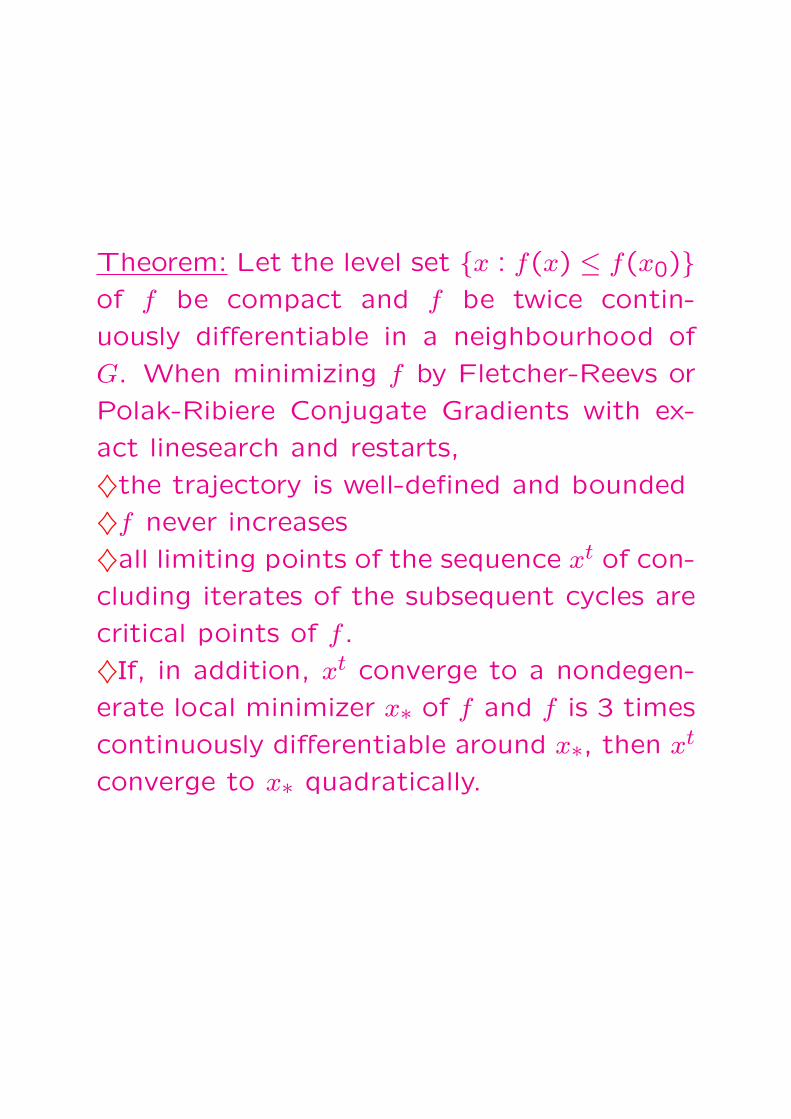
Theorem: Let the level set x : f(x) ≤ f(x0)of f be compact and f be twice contin-
uously differentiable in a neighbourhood of
G. When minimizing f by Fletcher-Reevs or
Polak-Ribiere Conjugate Gradients with ex-
act linesearch and restarts,
♦the trajectory is well-defined and bounded
♦f never increases
♦all limiting points of the sequence xt of con-
cluding iterates of the subsequent cycles are
critical points of f .
♦If, in addition, xt converge to a nondegen-
erate local minimizer x∗ of f and f is 3 times
continuously differentiable around x∗, then xt
converge to x∗ quadratically.
Quasi-Newton Methods
♣ Quasi-Newton methods are variable metric
methods of the generic form
xt+1 = xt − γt+1 St+1︸ ︷︷ ︸=A−1
t+1
f ′(xt)
where St+1 Â 0 and γt+1 is given by line-
search.
♠ In contrast to Modified Newton methods,
in Quasi-Newton algorithms one operates di-
rectly on matrix St+1, with the ultimate goal
to ensure, under favourable circumstances,
that
St+1 − [f ′′(xt)]−1 → 0, t →∞. (∗)
♠ In order to achieve (∗), in Quasi-Newton
methods one updates St into St+1 in a way
which ensures that
♦St+1 is  0
♦St+1(gt − gt−1) = xt − xt−1, where gτ =
f ′(xτ).

♣ Generic Quasi-Newton method:
Initialization: Choose somehow starting point
x0, matrix S1 Â 0, compute g0 = f ′(x0).
Step t: given xt−1, gt−1 = f ′(xt−1) and St Â0, terminate when gt−1 = 0, otherwise
♦Set dt = −Stgt−1 and perform exact line
search from xt−1 in the direction dt, thus get-
ting new iterate
xt = xt−1 + γtdt;
♦compute gt = f ′(xt) and set
pt = xt − xt−1, qt = gt − gt−1;
♦update St into positive definite symmetric
matrix St+1 in such a way that
St+1qt = pt
and loop.
♠ Requirements on the updating rule St 7→St+1:
♦In order for dt+1 to be direction of decrease
of f , the rule should ensure St+1 º 0
♦In the case of strongly convex quadratic f ,
the rule should ensure that St− [f ′′(·)]−1 → 0
as t →∞.

♠ Davidon-Fletcher-Powell method:
St+1 = St +1
pTt qt
ptpTt −
1
qTt Stqt
StqtqTt St.
♠ The Davidon-Fletcher-Powell method, as
applied to a strongly convex quadratic form,
finds exact solution in no more than n steps.
The trajectory generated by the method ini-
tialized with S1 = I is exactly the one of
the Conjugate Gradient method, so that
the DFP (Davidon-Fletcher-Powell) method
with the indicated initialization is a Conju-
gate Gradient method.
♣ The Broyden family.
Broyden-Fletcher-Goldfarb-Shanno updating
formula:
SBFGSt+1 = St+
1 + qTt Stqt
(pTt qt)2
ptpTt −
1
pTt qt
[ptq
Tt St + Stqtp
Tt
]
can be combined with the Davidon-Fletcher-
Powell formula
SDFPt+1 = St +
1
qTt pt
ptpTt −
1
qTt Stqt
StqtqTt St.
to yield a single-parametric Broyden family
of updating formulas
Sφt+1 = (1− φ)SDFP
t+1 + φSBFGSt+1
where φ ∈ [0,1] is parameter.

♣ Facts:
♦As applied to a strongly convex quadratic
form f , the Broyden method minimizes the
form exactly in no more than n steps, n be-
ing the dimension of the design vector. If S0
is proportional to the unit matrix, then the
trajectory of the method on f is exactly the
one of the Conjugate Gradient method.
♦all Broyden methods, independently of the
choice of the parameter φ, being started from
the same pair (x0, S1) and equipped with the
same exact line search and applied to the
same problem, generate the same sequence
of iterates (although not the same sequence
of matrices St!).
♣ Broyden methods are thought to be the
most efficient in practice versions of the Con-
jugate Gradient and quasi-Newton methods,
with the pure BFGS method (φ = 1) seem-
ingly being the best.

Convergence of Quasi-Newton methods
♣ Global convergence of Quasi-Newton meth-
ods without restarts is proved only for cer-
tain versions of the methods and only under
strong assumptions on f .
• For methods with restarts, where the
updating formulas are “refreshed” every m
steps by setting S = S0, one can easily prove
that under our standard assumption that the
level set G = x : f(x) ≤ f(x0) is com-
pact and f is continuously differentiable in a
neighbourhood of G, the trajectory of start-
ing points of the cycles is bounded, and all
its limiting points are critical points of f .
♣ Local convergence:
♦For scheme with restarts, one can prove
that if m = n and S0 = I, then the trajectory
of starting points xt of cycles, if it converges
to a nondegenerate local minimizer x∗ of f
such that f is 3 times continuously differen-
tiable around x∗, converges to x∗ quadrati-
cally.
♦Theorem [Powell, 1976]. Consider the
BFGS method without restarts and assume
that the method converges to a nondegener-
ate local minimizer x∗ of a three times con-
tinuously differentiable function f . Then the
method converges to x∗ superlinearly.
Convex Programming
♣ A Convex Programming program is an op-
timization program of the form
minX
f(x) (P)
where
• X ⊂ Rn is a convex compact set, intX 6= ∅;• f is a continuous convex function on Rn.

♠ Convexity of a set X ⊂ Rn means that
whenever X contains a pair of points x, y, it
contains the entire segment linking x and y:
x, y ∈ X ⇒ λx + (1− λ)y ∈ X ∀λ ∈ [0,1].
♠ Convexity of a function f : X → R de-
fined on a convex set X means that on every
segment in X, the function is below the cor-
responding secant:
x, y ∈ X, λ ∈ [0,1] ⇒f(λx + (1− λ)y) ≤ λf(x) + (1− λ)f(y).
Equivalently: The epigraph of f – the set
Epif = (x, t) : x ∈ X, t ≥ f(x) ⊂ Rn+1
– is convex.
minX
f(x) (P)
♣ Assume that our “environment” when
solving convex program (P) is as follows:
1. We have access to a Separation Oracle
Sep(X) for X – a routine which, given on
input a point x ∈ Rn, reports whether x ∈ X,
and in the case of x 6∈ X, returns a separator
– a vector e 6= 0 such that
eTx ≥ supy∈X
eTy
• Note: When X is convex and x 6∈ intX, a
separator does exist.

minX
f(x) (P)
2. We have access to a First Order oraclewhich, given on input a point x ∈ X, returnsthe value f(x) and a subgradient f ′(x) of f
at x.• A subgradient of f at x ∈ X is a vector g
such that
f(y) ≥ f(x) + gT (y − x) ∀y ∈ X.
Assuming f : X → R convex,• a subgradient exists at every pointx ∈ intX;• if f is differentiable at x ∈ X, thegradient ∇f(x) is a subgradient of f
at x (and this is the only subgradientof f at x, provided x ∈ intX);• if f is Lipschitz continuous on X,subgradient of f exists at every pointx ∈ X.

minX
f(x) (P)
3. We are given two positive reals R, r such
that for some (unknown) c one has
x : ‖x− c‖ ≤ r ⊂ X ⊂ x : ‖x‖2 ≤ R.
♠ Example: Consider an optimization pro-gram
minx∈X
f(x) ≡ max1≤`≤L
f`(x)
X = x ∈⊂ Rn : g(x) = max`=1,...,L
g`(x) ≤ 0where all f`, g` are convex differentiable func-tions on Rn.In this case
To build Separation and First Orderoracles is the same as to build a rou-tine which is capable to compute, ata given x, all f`(x), ∇f`(x), g`(x),∇g`(x).
Indeed, for a differentiable convex functionh, its gradient is a subgradient as well:
h(y) ≥ h(x) + (y − x)T∇h(x) ∀x, y,
and for the maximum h = max`=1,...,L
of convex
differentiable functions a subgradient at x isgiven by
∇h`(x)(x), `(x) : max`=1,...,L
h`(x) = h`(x)(x).

Thus,
• If we know how to compute f`, ∇f`, we
have in our disposal the First Order oracle
for f : we can take, as a subgradient of f at
x, the gradient of (any) function f` which is
the largest at x.
• If we know how to compute g`, ∇g`, we au-
tomatically have in our disposal a Separation
oracle for X.
Indeed, x ∈ X iff g(x) = max`=1,...,L
g`(x) ≤ 0.
Therefore
• In order to check whether x ∈ X, it
suffices to compute g(x) and to check
whether g(x) ≤ 0;
• In order to separate x from X when
x 6∈ X, it suffices
a) to find ` = `∗ such that g`(x) > 0
b) to set e = ∇g`∗(x).Indeed, we have
y ∈ X ⇒ [g`∗(x) + (y − x)T e ≤] g`∗(y) ≤ 0
⇒ eTy ≤ eTx− g`∗(x)≤ eTx.
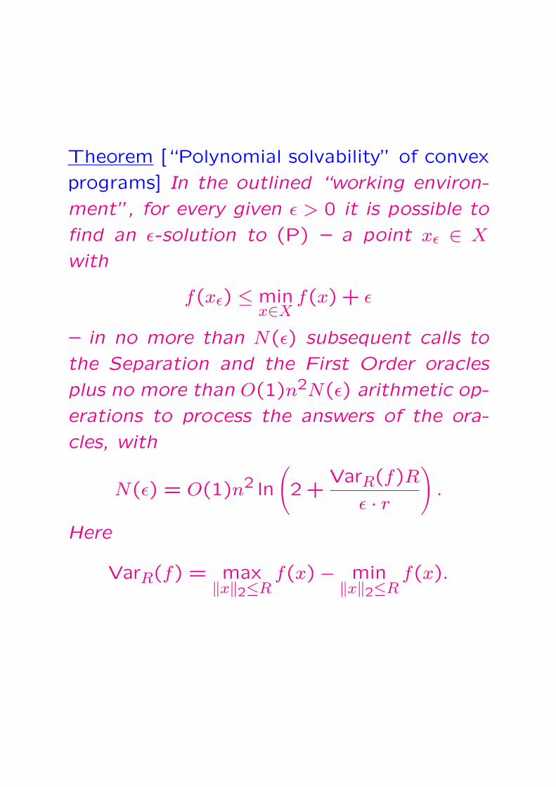
Theorem [“Polynomial solvability” of convex
programs] In the outlined “working environ-
ment”, for every given ε > 0 it is possible to
find an ε-solution to (P) – a point xε ∈ X
with
f(xε) ≤ minx∈X
f(x) + ε
– in no more than N(ε) subsequent calls to
the Separation and the First Order oracles
plus no more than O(1)n2N(ε) arithmetic op-
erations to process the answers of the ora-
cles, with
N(ε) = O(1)n2 ln
(2 +
VarR(f)R
ε · r
).
Here
VarR(f) = max‖x‖2≤R
f(x)− min‖x‖2≤R
f(x).
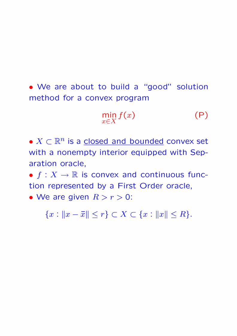
• We are about to build a “good” solution
method for a convex program
minx∈X
f(x) (P)
• X ⊂ Rn is a closed and bounded convex set
with a nonempty interior equipped with Sep-
aration oracle,
• f : X → R is convex and continuous func-
tion represented by a First Order oracle,
• We are given R > r > 0:
x : ‖x− x‖ ≤ r ⊂ X ⊂ x : ‖x‖ ≤ R.
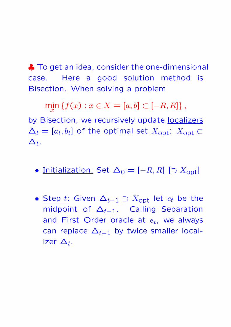
♣ To get an idea, consider the one-dimensional
case. Here a good solution method is
Bisection. When solving a problem
minxf(x) : x ∈ X = [a, b] ⊂ [−R, R] ,
by Bisection, we recursively update localizers
∆t = [at, bt] of the optimal set Xopt: Xopt ⊂∆t.
• Initialization: Set ∆0 = [−R, R] [⊃ Xopt]
• Step t: Given ∆t−1 ⊃ Xopt let ct be the
midpoint of ∆t−1. Calling Separation
and First Order oracle at et, we always
can replace ∆t−1 by twice smaller local-
izer ∆t.

“Given ∆t−1 ⊃ Xopt let ct be the midpoint
of ∆t−1. Calling Separation and First Order
oracle at et, we always can replace ∆t−1 by
twice smaller localizer ∆t:”
a b ct
1.a)
at−1
bt−1
f
a bct
1.b)
at−1
bt−1
f
ct
2.a)
at−1
bt−1
f
ct
2.b)
at−1
bt−1
f
ct
2.c)
at−1
bt−1
f
Bisection1) Sep(X) says that ct 6∈ X and says, via
separator e, on which side of ct X is.1.a): ∆t = [at−1, ct]; 1.b): ∆t = [ct, bt−1]
2) Sep(X) says that ct ∈ X, and O(f) says,via signf ′(ct), on which side of ct Xopt is.2.a): ∆t = [at−1, ct]; 2.b): ∆t = [ct, bt−1];2.c): ct ∈ Xopt

minx∈X
f(x) (P)
♣ In the multi-dimensional case, one can use
the Ellipsoid method – a simple generaliza-
tion of Bisection with ellipsoids playing the
role of segments.
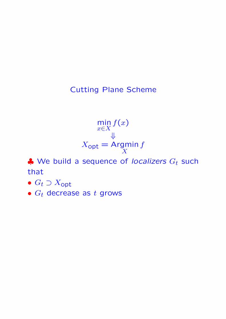
Cutting Plane Scheme
minx∈X
f(x)
⇓Xopt = Argmin
Xf
♣ We build a sequence of localizers Gt such
that
• Gt ⊃ Xopt
• Gt decrease as t grows
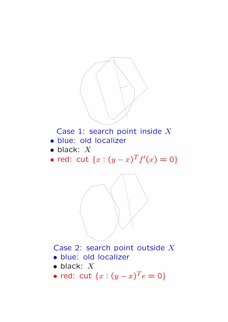
Case 1: search point inside X• blue: old localizer• black: X
• red: cut x : (y − x)Tf ′(x) = 0
Case 2: search point outside X• blue: old localizer• black: X
• red: cut x : (y − x)Te = 0

Straightforward implementation: Centers of
Gravity Method
• G0 = X
• xt =1
Vol(Gt−1)
∫
Gt−1
xdx
Theorem: For the Center of Gravity method,
one has
Vol(Gt) ≤(1−
(n
n+1
)n)Vol(Gt−1)
≤(1− 1
e
)Vol(Gt−1)
< 0.6322Vol(Gt−1).
(∗)
As a result,
mint≤T
f(xt)− f∗ ≤ (1− 1/e)T/nVarX(f)
Vol(Gt) ≤(1−
(n
n+1
)n)Vol(Gt−1)
≤(1− 1
e
)Vol(Gt−1)
< 0.6322Vol(Gt−1).
(∗)
♣ Reason for (*): Brunn-MinkowskiSymmeterization Principle:
Let Y be a convex compact set in Rn, ebe a unit direction and Z be “equi-cross-sectional” to X body symmetric w.r.t. e, sothat
• Z is symmetric w.r.t. the axis e
• for every hyperplane H = x : eTx =const, one has
Voln−1(X ∩H) = Voln−1(Z ∩H)
Then Z is a convex compact set.Equivalently: Let U, V be convex compactnonempty sets in Rn. Then
Vol1/n(U + V ) ≥ Vol1/n(U) + Vol1/n(V ).
In fact, convexity of U , V is redundant!

Why progress in volumes ensures progress in
accuracy?
♣ Let Vol(Gt) ≤ κVol(Gt−1) with κ < 1. We
claim that
mint≤T
f(xt)− f∗ ≤ κT/nVarX(f).
Indeed, let ν ∈ (κT/n,1), let x∗ = argminX
f
and let Xν = x∗ + ν(X − x∗).Then Vol(Xν) = νnVol(X) > κTVol(X) >
Vol(GT ), whence
Xν\GT 6= ∅.
We see that there exists z ∈ X such that
y ≡ x∗ + ν(z − x∗) 6∈ GT .
Thus, y ∈ Gt∗−1\Gt∗ for certain t∗ ≤ T , that
is,
(y − xt∗)Tf ′(xt∗) > 0 ⇒ f(xt∗) < f(y).
On the other hand,
f(y) = f(x∗ + ν(z − x∗))≤ f(x∗) + ν(f(z)− f(x∗))≤ f(x∗) + νVarX(f).
We see that
mint≤T
f(xt) ≤ f(xt∗) < f(y) ≤ f(x∗)+νVarX(f).
Passing to limits as ν → κT/n + 0, we arrive
at
mint≤T
f(xt) ≤ f(x∗) + κT/nVarX(f).
minx∈X
f(x) (P)
♣ Ellipsoid method – the idea. Assume we
already have an n-dimensional ellipsoid
E = x = c + Bu : uTu ≤ 1[B ∈ Rn×n,Det(B) 6= 0]
which covers the optimal set Xopt.
In order to replace E with a smaller ellipsoid
containing Xopt, we
1) Call Sep(X) to check whether c ∈ X
1.a) If Sep(X) says that c 6∈ X and returns a
separator e:
e 6= 0, eT c ≥ supy∈X
eTy.
we may be sure that
Xopt = Xopt⋂
E ⊂ E = x ∈ E : eT (x−c) ≤ 0.

1.b) If Sep(X) says that c ∈ X, we call O(f)
to compute f(c) and f ′(c), so that
f(y) ≥ f(c) + (y − c)Tf ′(c) ∀y (∗)
If f ′(c) = 0, c is optimal for (P) by (*), oth-
erwise (*) says that
Xopt = Xopt⋂
E ⊂ E = x ∈ E : [f ′(c)]︸ ︷︷ ︸e
T(x−c) ≤ 0
• Thus, we either terminate with optimal so-
lution, or get a “half-ellipsoid”
E = x ∈ E : eTx ≤ eT c [e 6= 0]
containing Xopt.

1) Given an ellipsoid
E = x = c + Bu : uTu ≤ 1[B ∈ Rn×n,Det(B) 6= 0]
containing the optimal set of (P) and callingthe Separation and the First Order oracles atthe center c of the ellipsoid, we pass from Eto the half-ellipsoid
E = x ∈ E : eTx ≤ eT c [e 6= 0]
containing Xopt.
2) It turns out that the half-ellipsoid E canbe included into a new ellipsoid E+ of n-dimensional volume less than the one of E:
E+ = x = c+ + B+u : uTu ≤ 1,c+ = c− 1
n+1Bp,
B+ = B
(n√
n2−1(In − ppT ) + n
n+1ppT)
= n√n2−1
B +(
nn+1 − n√
n2−1
)(Bp)pT ,
p = BT e√eT BBT e
Vol(E+) =(
n√n2−1
)n−1n
n+1Vol(E)
≤ exp−1/(2n)Vol(E)
♠ In the Ellipsoid method, we iterate the
above construction, starting with E0 = x :
‖x‖2 ≤ R ⊃ X, thus getting a sequence of el-
lipsoids Et+1 = (Et)+ with volumes “rapidly”
converging to 0, all of them containing Xopt.

♣ Verification of the fact that
E = x = c + Bu : uTu ≤ 1E = x ∈ E : eTx ≤ eT c
[e 6= 0]
⇓E ⊂ E+ = x = c+ + B+u : uTu ≤ 1
c+ = c− 1n+1Bp,
B+ = B
(n√
n2−1(In − ppT ) + n
n+1ppT)
= n√n2−1
B +(
nn+1 − n√
n2−1
)(Bp)pT ,
p = BT e√eT BBT e
is easy:
• E is the image of the unit ball under a one-
to-one affine mapping
• therefore E is the image of a half-ball W =
u : uTu ≤ 1, pTu ≤ 0 – under the same
mapping
• Ratio of volumes remains invariant under
affine mappings, and therefore all we need is
to find a “small” ellipsoid containing half-ball
W .
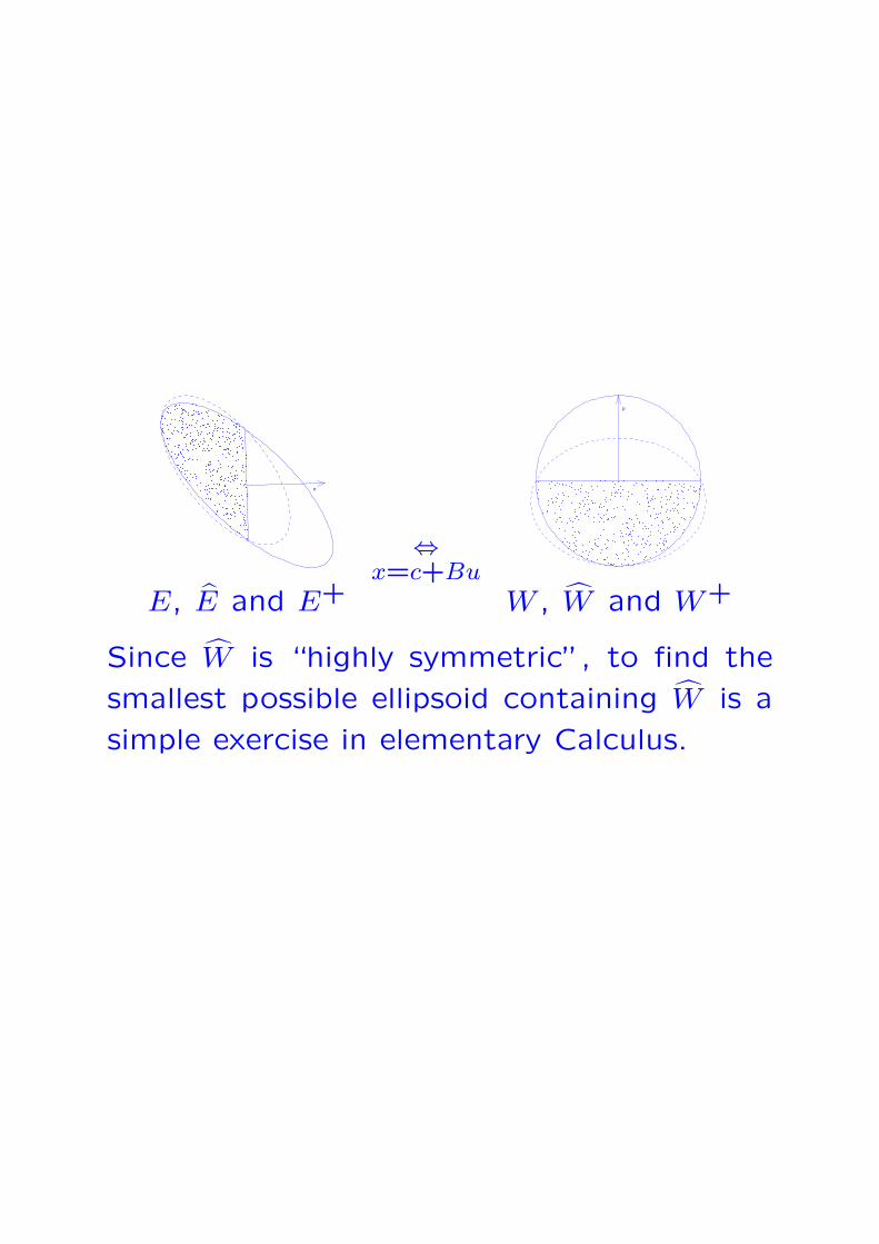
e
⇔x=c+Bu
p
E, E and E+ W , W and W+
Since W is “highly symmetric”, to find the
smallest possible ellipsoid containing W is a
simple exercise in elementary Calculus.
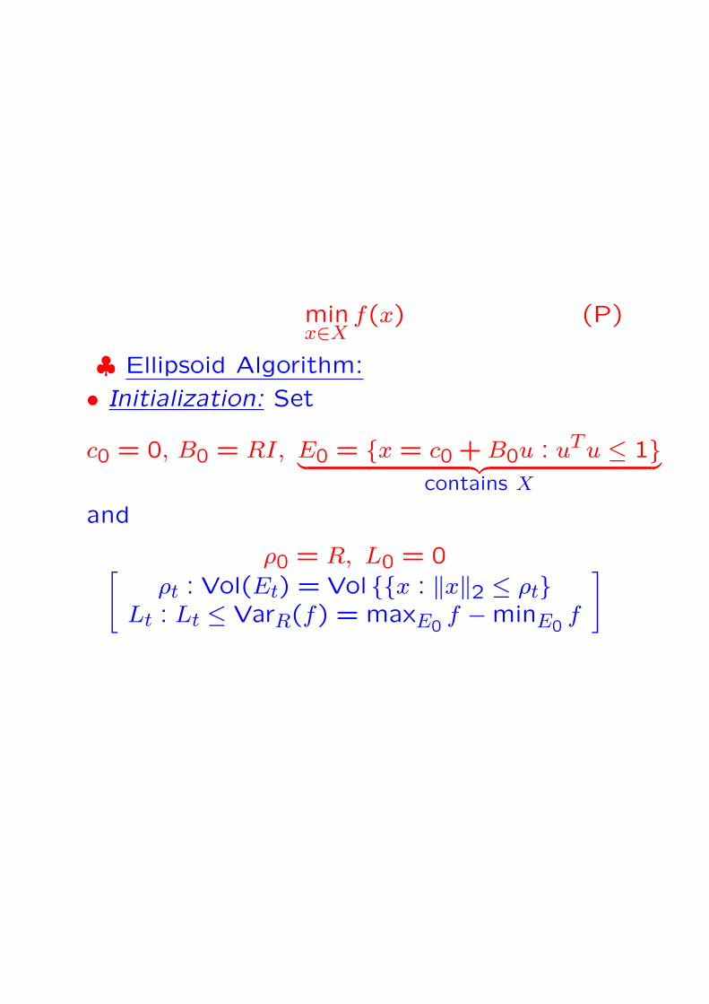
minx∈X
f(x) (P)
♣ Ellipsoid Algorithm:
• Initialization: Set
c0 = 0, B0 = RI, E0 = x = c0 + B0u : uTu ≤ 1︸ ︷︷ ︸contains X
and
ρ0 = R, L0 = 0[ρt : Vol(Et) = Vol x : ‖x‖2 ≤ ρt
Lt : Lt ≤ VarR(f) = maxE0f −minE0
f
]

Step t, t = 1,2, .... At the beginning of step
t, we have the data ct−1, Bt−1 of the previous
ellipsoid
Et−1 = x = ct−1 + Bt−1u : uTu ≤ 1[ct−1 ∈ Rn, Bt−1 ∈ Rn×n,DetBt−1 6= 0]
along with the quantities Lt−1 ≥ 0 and ρt−1.
• At step t,
1) We call Sep(X), ct−1 being the input. If
xt−1 6∈ X (“non-productive step”), Sep(X)
returns a separator
e 6= 0 : eT ct−1 ≥ supy∈X
eTy.
In this case, we set
et = e, Lt = Lt−1
and go to 3). If ct−1 ∈ X (“productive
step”), we go to 2).

2) We call O(f), ct−1 being the input, to get
f(ct−1), e = f ′(ct−1). If e = 0, we terminate
and claim that ct−1 is an optimal solution to
(P).
If e 6= 0, we set
et = e,
compute the quantity
`t = maxy∈E0
[eTt y − eT
t ct−1] = R‖et‖2 − eTt ct−1,
update L by setting
Lt = maxLt−1, `tand go to 3).
Note: Since f(y)−f(ct−1) ≥ eTt (y−ct−1), and
ct−1 ∈ X ⊂ E0, we have `t ≤ maxE0f(y) −
f(ct−1) ≤ VarR(f), whence Lt ≤ VarR(f).
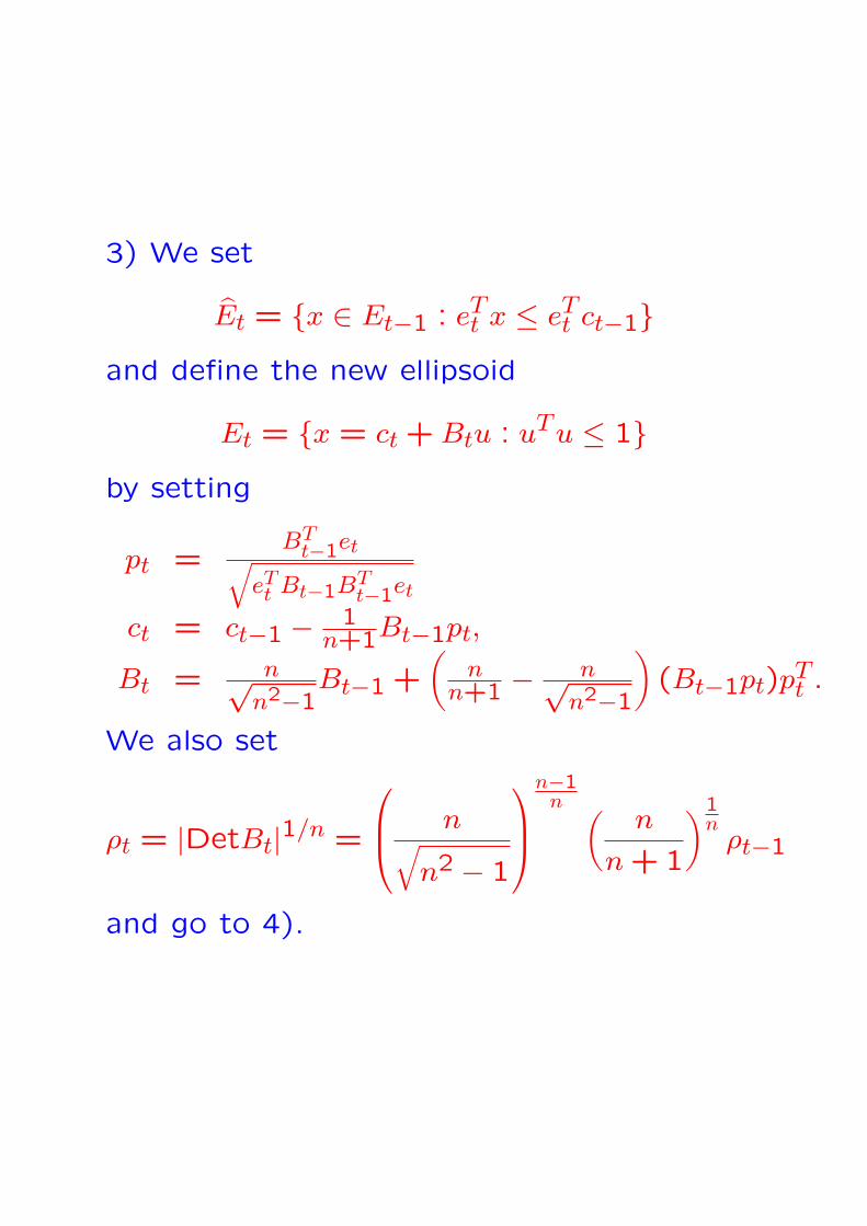
3) We set
Et = x ∈ Et−1 : eTt x ≤ eT
t ct−1and define the new ellipsoid
Et = x = ct + Btu : uTu ≤ 1by setting
pt =BT
t−1et√eTt Bt−1BT
t−1et
ct = ct−1 − 1n+1Bt−1pt,
Bt = n√n2−1
Bt−1 +(
nn+1 − n√
n2−1
)(Bt−1pt)pT
t .
We also set
ρt = |DetBt|1/n =
n√n2 − 1
n−1n (
n
n + 1
)1n
ρt−1
and go to 4).

4) [Termination test]. We check whether the
inequalityρt
r<
ε
Lt + ε(∗)
(r > 0 is a given in advance radius of Euclid-
ean ball contained in X).
• If (*) holds, we terminate and output the
best (with the smallest value of f) of the
“search points” cτ−1 associated with produc-
tive steps τ ≤ t.
• If (*) does not hold, we pass to step t +1.

Numerical example:
min f(x),f(x) = 1
2(1.4435x1 + 0.6232x2 − 7.9574)2
+5(−0.3509x1 + 0.7990x2 + 2.8778)4
−1 ≤ x1, x2 ≤ 1,
• Xopt = (1,−1), Opt = 70.030152768...
Here are the best objective values of feasible
solutions found in course of the first t steps,
t = 1, ...,256:
t best value t best value1 374.61091739 16 76.8382534512 216.53084103 ... ...3 146.74723394 32 70.9013448154 112.42945457 ... ...5 93.84206347 64 70.0316334836 82.90928589 ... ...7 82.90928589 128 70.0301541928 82.90928589 ... ...... ... 256 70.030152768
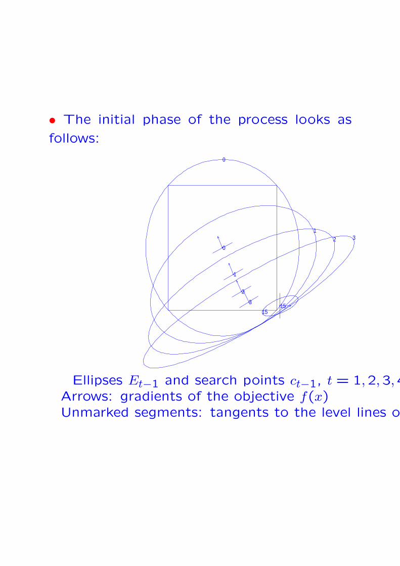
• The initial phase of the process looks as
follows:
0
0
1
1
2
2
3
3
1515
Ellipses Et−1 and search points ct−1, t = 1,2,3,4,16Arrows: gradients of the objective f(x)Unmarked segments: tangents to the level lines of f(x)
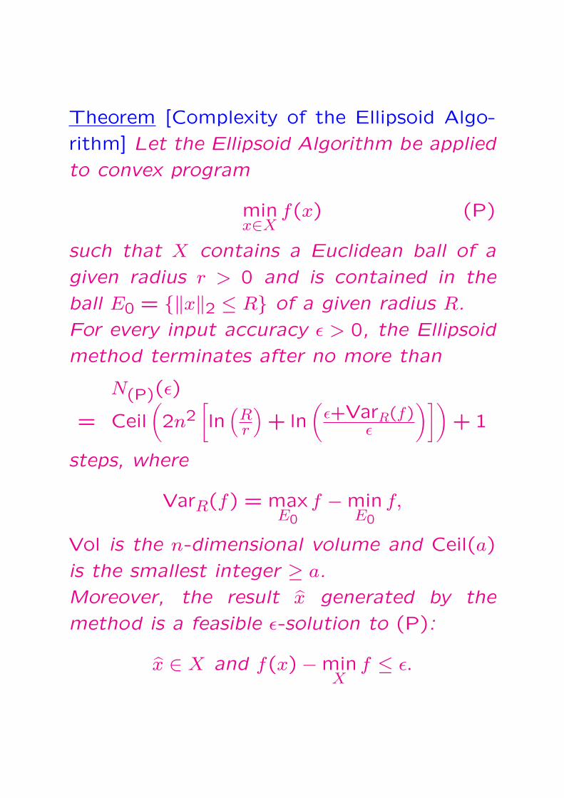
Theorem [Complexity of the Ellipsoid Algo-
rithm] Let the Ellipsoid Algorithm be applied
to convex program
minx∈X
f(x) (P)
such that X contains a Euclidean ball of a
given radius r > 0 and is contained in the
ball E0 = ‖x‖2 ≤ R of a given radius R.
For every input accuracy ε > 0, the Ellipsoid
method terminates after no more than
N(P)(ε)
= Ceil(2n2
[ln
(Rr
)+ ln
(ε+VarR(f)
ε
)])+ 1
steps, where
VarR(f) = maxE0
f −minE0
f,
Vol is the n-dimensional volume and Ceil(a)
is the smallest integer ≥ a.
Moreover, the result x generated by the
method is a feasible ε-solution to (P):
x ∈ X and f(x)−minX
f ≤ ε.
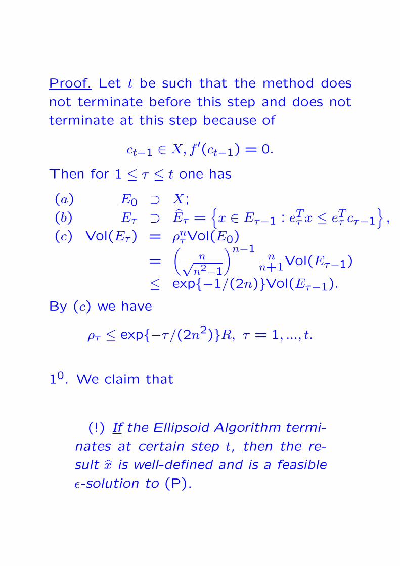
Proof. Let t be such that the method does
not terminate before this step and does not
terminate at this step because of
ct−1 ∈ X, f ′(ct−1) = 0.
Then for 1 ≤ τ ≤ t one has
(a) E0 ⊃ X;
(b) Eτ ⊃ Eτ =x ∈ Eτ−1 : eT
τ x ≤ eTτ cτ−1
,
(c) Vol(Eτ) = ρnτVol(E0)
=(
n√n2−1
)n−1n
n+1Vol(Eτ−1)
≤ exp−1/(2n)Vol(Eτ−1).
By (c) we have
ρτ ≤ exp−τ/(2n2)R, τ = 1, ..., t.
10. We claim that
(!) If the Ellipsoid Algorithm termi-
nates at certain step t, then the re-
sult x is well-defined and is a feasible
ε-solution to (P).

(!) “If the Ellipsoids method terminates at
certain step t, then the result x is well-defined
and is a feasible ε-solution to (P).”
Indeed, there are two possible reasons for ter-
mination at step t:
• We arrive at the situation where
ct−1 ∈ X and f ′(ct−1) = 0. (A)
In this case
∀y : f(y) ≥ f(ct−1)+(y−ct−1)Tf ′(ct−1) = f(ct−1),
and since ct−1 ∈ X, ct−1 is optimal solution
to minX
f .
• We arrive at the situation where
ρt
r<
ε
Lt + ε(B)
Let us prove that (!) is valid in the case of
(B).
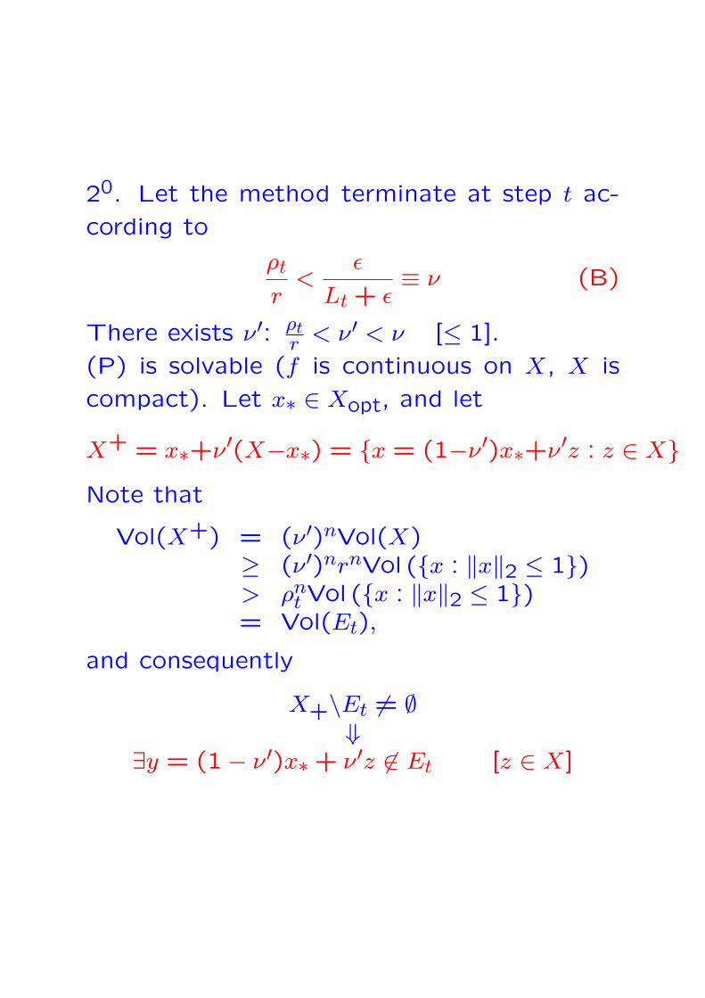
20. Let the method terminate at step t ac-
cording to
ρt
r<
ε
Lt + ε≡ ν (B)
There exists ν′: ρtr < ν′ < ν [≤ 1].
(P) is solvable (f is continuous on X, X is
compact). Let x∗ ∈ Xopt, and let
X+ = x∗+ν′(X−x∗) = x = (1−ν′)x∗+ν′z : z ∈ XNote that
Vol(X+) = (ν′)nVol(X)≥ (ν′)nrnVol (x : ‖x‖2 ≤ 1)> ρn
t Vol (x : ‖x‖2 ≤ 1)= Vol(Et),
and consequently
X+\Et 6= ∅⇓
∃y = (1− ν′)x∗ + ν′z 6∈ Et [z ∈ X]
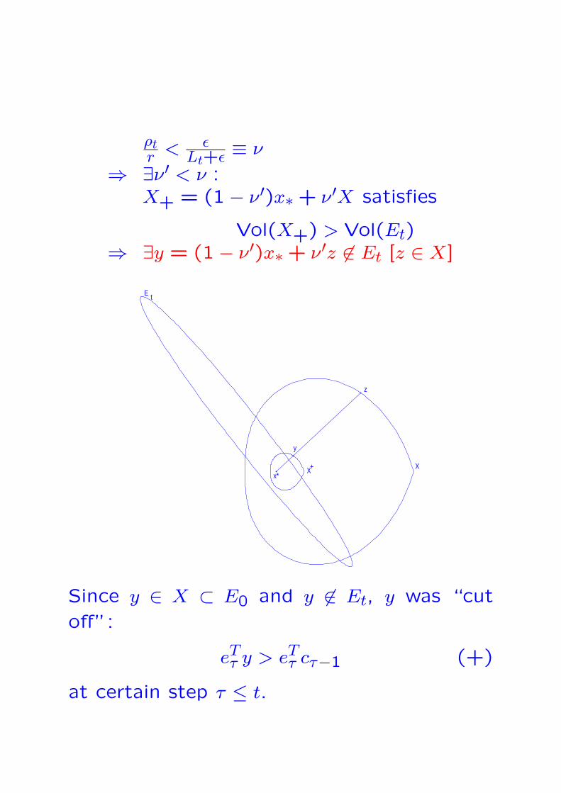
ρtr < ε
Lt+ε ≡ ν
⇒ ∃ν′ < ν :X+ = (1− ν′)x∗ + ν′X satisfies
Vol(X+) > Vol(Et)⇒ ∃y = (1− ν′)x∗ + ν′z 6∈ Et [z ∈ X]
x*XX+
z
y
E t
Since y ∈ X ⊂ E0 and y 6∈ Et, y was “cut
off”:
eTτ y > eT
τ cτ−1 (+)
at certain step τ ≤ t.
• Exists τ ≤ t:
eTτ y > eT
τ cτ−1 (+)
Observe that the step τ is productive, since
otherwise eτ separates cτ−1 and X, while y ∈X. Consequently, eτ = f ′(cτ−1).

• Situation: We are solving problem
minx∈X
f(x) (P)
and the Ellipsoid Algorithm terminates at
step t.
• Target: To prove that the result is an ε-
solution to (P)
• Current state of the proof: We are explor-
ing the case
∃y = (1−ν′)x∗+ν′z[x∗ ∈ Xopt, z ∈ X, ν′ < ε
Lt + ε
]
and a productive step τ ≤ t such that
(y − cτ−1)Tf ′(cτ−1) > 0 (+)
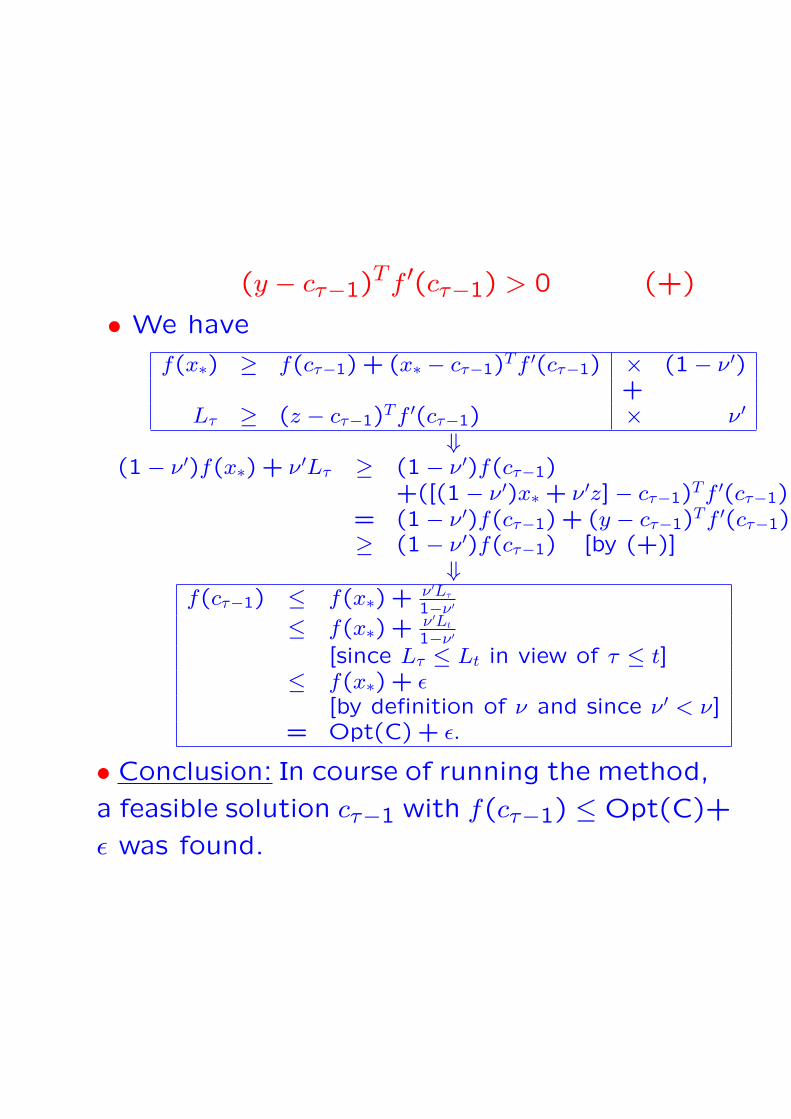
(y − cτ−1)Tf ′(cτ−1) > 0 (+)
• We have
f(x∗) ≥ f(cτ−1) + (x∗ − cτ−1)Tf ′(cτ−1) × (1− ν ′)+
Lτ ≥ (z − cτ−1)Tf ′(cτ−1) × ν ′
⇓(1− ν ′)f(x∗) + ν ′Lτ ≥ (1− ν ′)f(cτ−1)
+([(1− ν ′)x∗ + ν ′z]− cτ−1)Tf ′(cτ−1)= (1− ν ′)f(cτ−1) + (y − cτ−1)Tf ′(cτ−1)≥ (1− ν ′)f(cτ−1) [by (+)]
⇓f(cτ−1) ≤ f(x∗) + ν ′Lτ
1−ν ′
≤ f(x∗) + ν ′Lt
1−ν ′
[since Lτ ≤ Lt in view of τ ≤ t]≤ f(x∗) + ε
[by definition of ν and since ν ′ < ν]= Opt(C) + ε.
• Conclusion: In course of running the method,
a feasible solution cτ−1 with f(cτ−1) ≤ Opt(C)+
ε was found.
• Situation: We are solving problem
minx∈X
f(x) (P)
and the Ellipsoid Algorithm terminates at
step t.
• Target: To prove that the result is an ε-
solution to (P)
• Current state of the proof: It was shown
that in course of running the method, a fea-
sible solution cτ−1 with f(cτ−1) ≤ Opt(C)+ ε
was found.
• By construction, the result of the Ellip-
soid Algorithm is the best – with the smallest
value of f – of feasible solutions cs−1 gen-
erated in course of t steps, so that if the
method terminates at a step t, then the re-
sult is an ε-solution to (P).
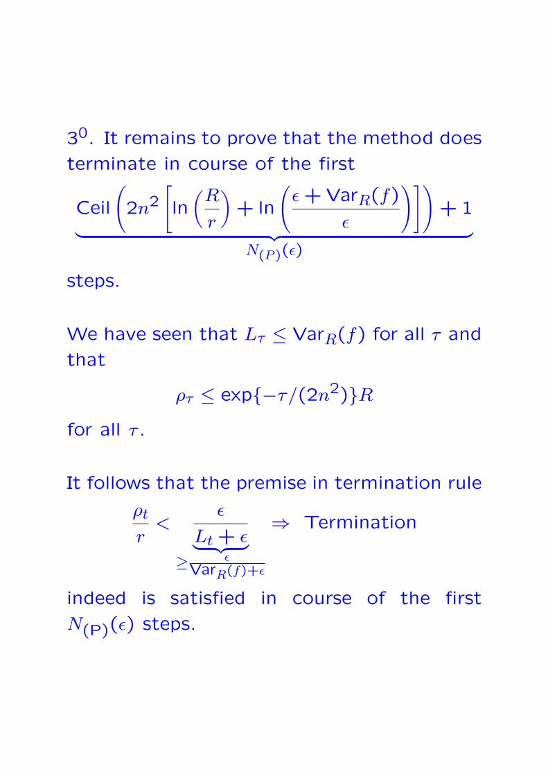
30. It remains to prove that the method does
terminate in course of the first
Ceil
(2n2
[ln
(R
r
)+ ln
(ε + VarR(f)
ε
)])+ 1
︸ ︷︷ ︸N(P )(ε)
steps.
We have seen that Lτ ≤ VarR(f) for all τ and
that
ρτ ≤ exp−τ/(2n2)Rfor all τ .
It follows that the premise in termination rule
ρt
r<
ε
Lt + ε︸ ︷︷ ︸≥ ε
VarR(f)+ε
⇒ Termination
indeed is satisfied in course of the first
N(P)(ε) steps.
♣ Traditional methods for general constrained
problems
minx
f(x) :
gj(x) ≤ 0, j = 1, ..., mhi(x) = 0, i = 1, ..., k
(P )
can be partitioned into
♦Primal methods, where one mimics uncon-
strained approach, travelling along the fea-
sible set in a way which ensures progress in
objective at every step
♦Penalty/Barrier methods, which reduce con-
strained minimization to solving a sequence
of essentially unconstrained problems
♦Lagrange Multiplier methods, where one
focuses on dual problem associated with (P ).
A posteriori the Lagrange multiplier meth-
ods, similarly to the penalty/barrier ones,
reduce (P ) to a sequence of unconstrained
problems, but in a “smart” manner different
from the penalty/barrier scheme
♦Sequential Quadratic Programming meth-
ods, where one directly solves the KKT sys-
tem associated with (P ) by a kind of Newton
method.
Penalty/Barrier Methods
♣ Penalty Scheme, Equality Constrainsts. Con-
sider equality constrained problem
minxf(x) : hi(x) = 0, i = 1, ..., k (P )
and let us “approximate” it by unconstrained
problem
minx
fρ(x) = f(x) +ρ
2
k∑
i=1
h2i (x)
︸ ︷︷ ︸penaltyterm
(P [ρ])
ρ > 0 is penalty parameter.
Note: (A) On the feasible set, the penalty
term vanishes, thus fρ ≡ f ;
(B) When ρ is large and x is infeasible, fρ(x)
is large:
limρ→∞ fρ(x) =
f(x), x is feasible+∞, otherwise
⇒ It is natural to expect that solution of
(P [ρ]) approaches, as ρ → ∞, the optimal
set of (P ).

♣ Penalty Scheme, General Constraints. In
the case of general constrained problem
minx
f(x) :
hi(x) = 0, i = 1, ..., kgj ≤ 0, j = 1, ..., m
, (P )
the same idea of penalizing the constraint vi-
olations results in approximating (P ) by un-
constrained problem
minx
fρ(x) = f(x)+ρ
2
k∑
i=1
h2i (x) +
m∑
j=1
[gj(x)+]2
︸ ︷︷ ︸penaltyterm
(P [ρ])
where
g+j (x) = max[gj(x),0]
and ρ > 0 is penalty parameter. Here again
limρ→∞ fρ(x) =
f(x), x is feasible+∞, otherwise
and we again may expect that the solutions
of (P [ρ]) approach, as ρ → ∞, the optimal
set of (P ).

♣ Barrier scheme normally is used for in-
equality constrained problems
minx
f(x) : gj(x) ≤ 0, j = 1, ..., m
(P )
satisfying “Slater condition”: the feasible set
G =x : gj(x) ≤ 0, j ≤ m
of (P ) possesses a nonempty interior intG
which is dense in G, and gj(x) < 0 for x ∈intG.
♠ Given (P ), one builds a barrier (≡interior
penalty) for G – a function F which is well-
defined and smooth on intG and blows up to
+∞ along every sequence of points xi ∈ intG
converging to a boundary point of G:
xi ∈ intG, limi→∞xi = x 6∈ intG ⇒ F (xi) →∞, i →∞.
Examples:
♦Log-barrier F (x) = −∑j
ln(−gj(x))
♦Carrol Barrier F (x) = −∑j
1gj(x)
minx
f(x) : gj(x) ≤ 0, j = 1, ..., m
(P )
♠ After interior penalty F for the feasible do-
main of (P ) is chosen, the problem is approx-
imated by the “essentially unconstrained”
problem
minx∈intG
Fρ(x) = f(x) +1
ρF (x) (P [ρ])
When penalty parameter ρ is large, the func-
tion Fρ is close to f everywhere in G, except
for a thin stripe around the boundary.
⇒ It is natural to expect that solutions of
(P [ρ]) approach the optimal set of (P ) as
ρ →∞,

Investigating Penalty Scheme
♣ Let us focus on equality constrained prob-
lem
minxf(x) : hi(x) = 0, i = 1, ..., k (P )
and associated penalized problems
minx
fρ(x) = f(x) +ρ
2‖h(x)‖22 (P [ρ])
(results for general case are similar).
♠ Questions of interest:
♦Whether indeed unconstrained minimizers
of the penalized objective fρ converge, as
ρ →∞, to the optimal set of (P )?
♦What are our possibilities to minimize the
penalized objective?

minxf(x) : hi(x) = 0, i = 1, ..., k (P )
⇓min
xfρ(x) = f(x) + ρ
2‖h(x)‖22 (P [ρ])
Simple fact: Let (P ) be feasible, the objec-
tive and the constraints in (P ) be contin-
uous and let f possess bounded level sets
x : f(x) ≤ a. Let, further X∗ be the
set of global solutions to (P ). Then X∗is nonempty, approximations problems (P [ρ])
are solvable, and their global solutions ap-
proach X∗ as ρ →∞:
∀ε > 0∃ρ(ε) : ρ ≥ ρ(ε), x∗(ρ) solves (P [ρ])⇒ dist(x∗(ρ), X∗) ≡ min
x∗∈X∗‖x∗(ρ)− x∗‖2 ≤ ε
Proof. 10. By assumption, the feasible set
of (P ) is nonempty and closed, f is contin-
uous and f(x) → ∞ as ‖x‖2 → ∞. It follows
that f attains its minimum on the feasible
set, and the set X∗ of global minimizers of f
on the feasible set is bounded and closed.

minxf(x) : hi(x) = 0, i = 1, ..., k (P )
⇓min
xfρ(x) = f(x) + ρ
2‖h(x)‖22 (P [ρ])
20. The objective in (P [ρ]) is continuous
and goes to +∞ as ‖x‖2 →∞; consequently,
(P [ρ]) is solvable.
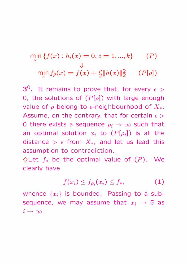
minxf(x) : hi(x) = 0, i = 1, ..., k (P )
⇓min
xfρ(x) = f(x) + ρ
2‖h(x)‖22 (P [ρ])
30. It remains to prove that, for every ε >
0, the solutions of (P [ρ]) with large enough
value of ρ belong to ε-neighbourhood of X∗.Assume, on the contrary, that for certain ε >
0 there exists a sequence ρi → ∞ such that
an optimal solution xi to (P [ρi]) is at the
distance > ε from X∗, and let us lead this
assumption to contradiction.
♦Let f∗ be the optimal value of (P ). We
clearly have
f(xi) ≤ fρi(xi) ≤ f∗, (1)
whence xi is bounded. Passing to a sub-
sequence, we may assume that xi → x as
i →∞.
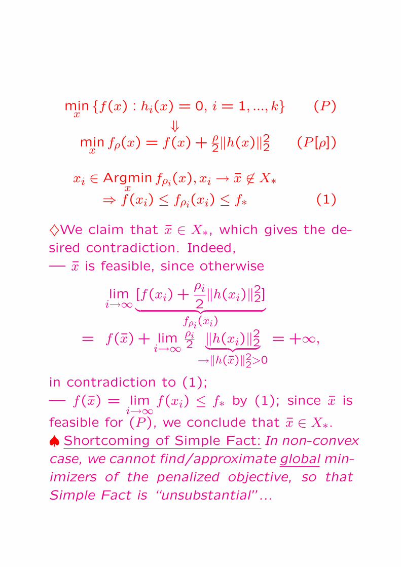
minxf(x) : hi(x) = 0, i = 1, ..., k (P )
⇓min
xfρ(x) = f(x) + ρ
2‖h(x)‖22 (P [ρ])
xi ∈ Argminx
fρi(x), xi → x 6∈ X∗⇒ f(xi) ≤ fρi(xi) ≤ f∗ (1)
♦We claim that x ∈ X∗, which gives the de-
sired contradiction. Indeed,
— x is feasible, since otherwise
limi→∞ [f(xi) +
ρi
2‖h(xi)‖22]︸ ︷︷ ︸
fρi(xi)
= f(x) + limi→∞
ρi2 ‖h(xi)‖22︸ ︷︷ ︸→‖h(x)‖22>0
= +∞,
in contradiction to (1);
— f(x) = limi→∞ f(xi) ≤ f∗ by (1); since x is
feasible for (P ), we conclude that x ∈ X∗.♠ Shortcoming of Simple Fact: In non-convex
case, we cannot find/approximate global min-
imizers of the penalized objective, so that
Simple Fact is “unsubstantial”...
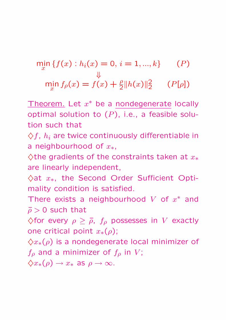
minxf(x) : hi(x) = 0, i = 1, ..., k (P )
⇓min
xfρ(x) = f(x) + ρ
2‖h(x)‖22 (P [ρ])
Theorem. Let x∗ be a nondegenerate locally
optimal solution to (P ), i.e., a feasible solu-
tion such that
♦f , hi are twice continuously differentiable in
a neighbourhood of x∗,♦the gradients of the constraints taken at x∗are linearly independent,
♦at x∗, the Second Order Sufficient Opti-
mality condition is satisfied.
There exists a neighbourhood V of x∗ and
ρ > 0 such that
♦for every ρ ≥ ρ, fρ possesses in V exactly
one critical point x∗(ρ);♦x∗(ρ) is a nondegenerate local minimizer of
fρ and a minimizer of fρ in V ;
♦x∗(ρ) → x∗ as ρ →∞.
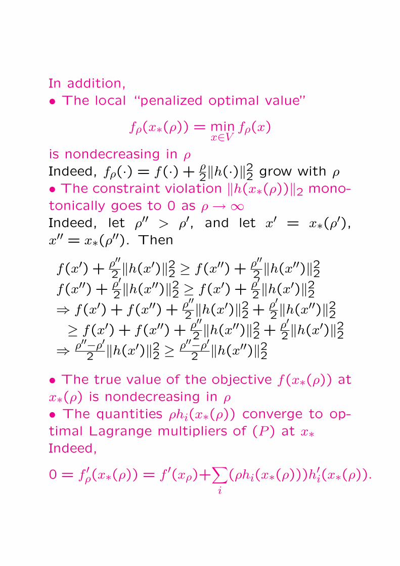
In addition,• The local “penalized optimal value”
fρ(x∗(ρ)) = minx∈V
fρ(x)
is nondecreasing in ρ
Indeed, fρ(·) = f(·) + ρ2‖h(·)‖22 grow with ρ
• The constraint violation ‖h(x∗(ρ))‖2 mono-tonically goes to 0 as ρ →∞Indeed, let ρ′′ > ρ′, and let x′ = x∗(ρ′),x′′ = x∗(ρ′′). Then
f(x′) + ρ′′2 ‖h(x′)‖22 ≥ f(x′′) + ρ′′
2 ‖h(x′′)‖22f(x′′) + ρ′
2‖h(x′′)‖22 ≥ f(x′) + ρ′2‖h(x′)‖22
⇒ f(x′) + f(x′′) + ρ′′2 ‖h(x′)‖22 + ρ′
2‖h(x′′)‖22≥ f(x′) + f(x′′) + ρ′′
2 ‖h(x′′)‖22 + ρ′2‖h(x′)‖22
⇒ ρ′′−ρ′2 ‖h(x′)‖22 ≥ ρ′′−ρ′
2 ‖h(x′′)‖22• The true value of the objective f(x∗(ρ)) atx∗(ρ) is nondecreasing in ρ
• The quantities ρhi(x∗(ρ)) converge to op-timal Lagrange multipliers of (P ) at x∗Indeed,
0 = f ′ρ(x∗(ρ)) = f ′(xρ)+∑
i
(ρhi(x∗(ρ)))h′i(x∗(ρ)).
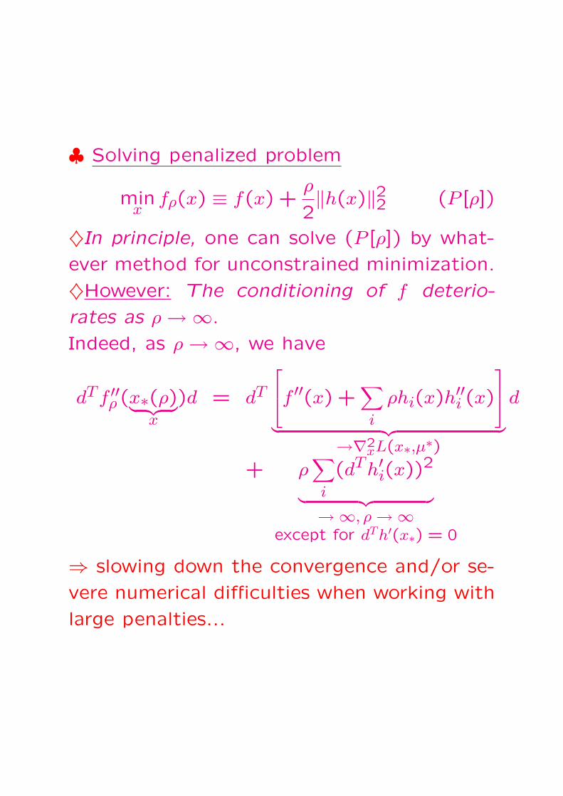
♣ Solving penalized problem
minx
fρ(x) ≡ f(x) +ρ
2‖h(x)‖22 (P [ρ])
♦In principle, one can solve (P [ρ]) by what-
ever method for unconstrained minimization.
♦However: The conditioning of f deterio-
rates as ρ →∞.
Indeed, as ρ →∞, we have
dTf ′′ρ (x∗(ρ)︸ ︷︷ ︸x
)d = dT
f ′′(x) +
∑
i
ρhi(x)h′′i (x)
︸ ︷︷ ︸→∇2
xL(x∗,µ∗)
d
+ ρ∑
i
(dTh′i(x))2
︸ ︷︷ ︸→∞, ρ →∞
except for dTh′(x∗) = 0
⇒ slowing down the convergence and/or se-
vere numerical difficulties when working with
large penalties...
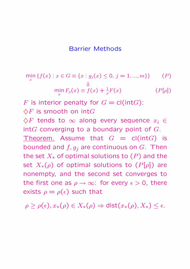
Barrier Methods
minxf(x) : x ∈ G ≡ x : gj(x) ≤ 0, j = 1, ..., m (P )
⇓min
xFρ(x) ≡ f(x) + 1
ρF (x) (P [ρ])
F is interior penalty for G = cl(intG):
♦F is smooth on intG
♦F tends to ∞ along every sequence xi ∈intG converging to a boundary point of G.
Theorem. Assume that G = cl(intG) is
bounded and f, gj are continuous on G. Then
the set X∗ of optimal solutions to (P ) and the
set X∗(ρ) of optimal solutions to (P [ρ]) are
nonempty, and the second set converges to
the first one as ρ →∞: for every ε > 0, there
exists ρ = ρ(ε) such that
ρ ≥ ρ(ε), x∗(ρ) ∈ X∗(ρ) ⇒ dist(x∗(ρ), X∗) ≤ ε.

♣ In the case of convex program
minx∈G
f(x) (P )
with closed and bounded convex G and con-
vex objective f , the domain G can be in many
ways equipped with a twice continuously dif-
ferentiable strongly convex penalty F (x).
♠ Assuming f twice continuously differen-
tiable on intG, the aggregate
Fρ(x) = ρf(x) + F (x)
is strongly convex on intG and therefore at-
tains its minimum at a single point
x∗(ρ) = argminx∈intG
Fρ(x).
♠ It is easily seen that the path x∗(ρ) is
continuously differentiable and converges, as
ρ →∞, to the optimal set of (P ).
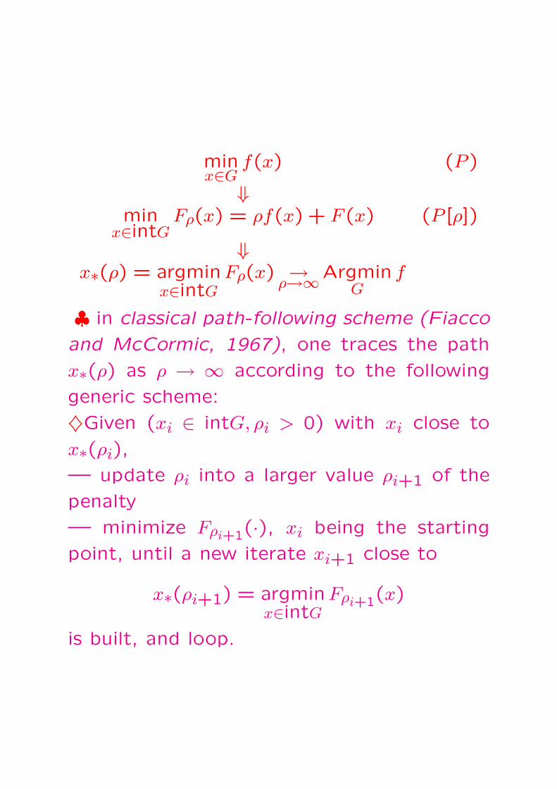
minx∈G
f(x) (P )
⇓min
x∈intGFρ(x) = ρf(x) + F (x) (P [ρ])
⇓x∗(ρ) = argmin
x∈intGFρ(x) →
ρ→∞ArgminG
f
♣ in classical path-following scheme (Fiacco
and McCormic, 1967), one traces the path
x∗(ρ) as ρ → ∞ according to the following
generic scheme:
♦Given (xi ∈ intG, ρi > 0) with xi close to
x∗(ρi),
— update ρi into a larger value ρi+1 of the
penalty
— minimize Fρi+1(·), xi being the starting
point, until a new iterate xi+1 close to
x∗(ρi+1) = argminx∈intG
Fρi+1(x)
is built, and loop.
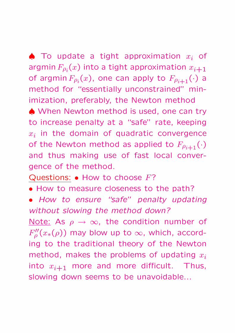
♠ To update a tight approximation xi of
argminFρi(x) into a tight approximation xi+1
of argminFρi(x), one can apply to Fρi+1(·) a
method for “essentially unconstrained” min-
imization, preferably, the Newton method
♠ When Newton method is used, one can try
to increase penalty at a “safe” rate, keeping
xi in the domain of quadratic convergence
of the Newton method as applied to Fρi+1(·)and thus making use of fast local conver-
gence of the method.
Questions: • How to choose F?
• How to measure closeness to the path?
• How to ensure “safe” penalty updating
without slowing the method down?
Note: As ρ → ∞, the condition number of
F ′′ρ (x∗(ρ)) may blow up to ∞, which, accord-
ing to the traditional theory of the Newton
method, makes the problems of updating xi
into xi+1 more and more difficult. Thus,
slowing down seems to be unavoidable...

♣ In late 80’s, it was discovered that the clas-
sical path-following scheme, associated with
properly chosen barriers, admits “safe” im-
plementation without slowing down. This
discovery led to invention of Polynomial
Time Interior Point methods for convex pro-
grams.
♣ Majority of Polynomial Time Interior Point
methods heavily exploit the classical path-
following scheme; the novelty is in what
are the underlying barriers – these are spe-
cific self-concordant functions especially well
suited for Newton minimization.
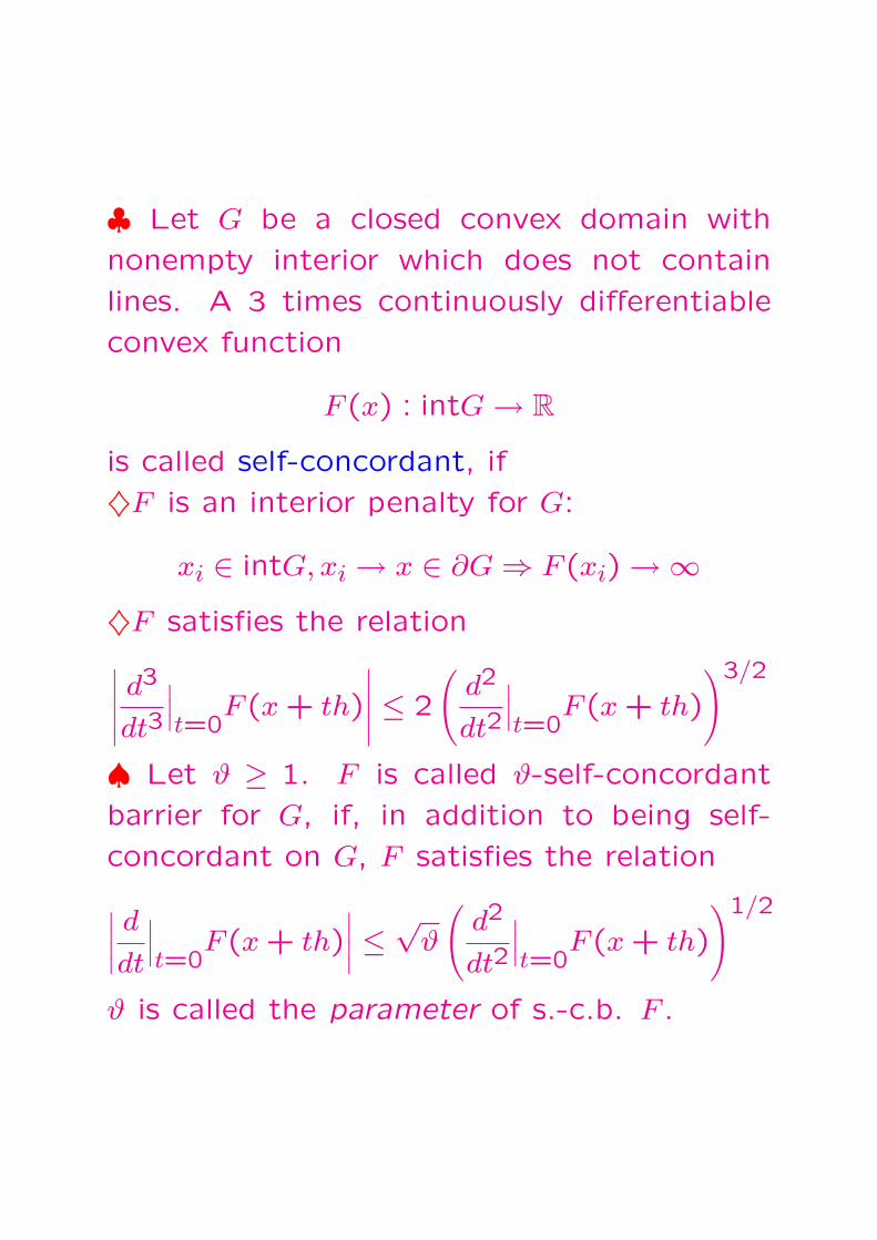
♣ Let G be a closed convex domain with
nonempty interior which does not contain
lines. A 3 times continuously differentiable
convex function
F (x) : intG → R
is called self-concordant, if
♦F is an interior penalty for G:
xi ∈ intG, xi → x ∈ ∂G ⇒ F (xi) →∞♦F satisfies the relation∣∣∣∣∣d3
dt3
∣∣∣t=0
F (x + th)
∣∣∣∣∣ ≤ 2
(d2
dt2
∣∣∣t=0
F (x + th)
)3/2
♠ Let ϑ ≥ 1. F is called ϑ-self-concordant
barrier for G, if, in addition to being self-
concordant on G, F satisfies the relation
∣∣∣∣d
dt
∣∣∣t=0
F (x + th)∣∣∣∣ ≤
√ϑ
(d2
dt2
∣∣∣t=0
F (x + th)
)1/2
ϑ is called the parameter of s.-c.b. F .

♣ Every convex program
minx∈G
f(x)
can be converted into a convex program with
linear objective, namely,
mint,x
t : x ∈ G, f(x) ≤ t .
Assuming that this transformation has been
done at the very beginning, we can w.l.o.g.
focus on convex program with linear objec-
tive
minx∈G
cTx (P )
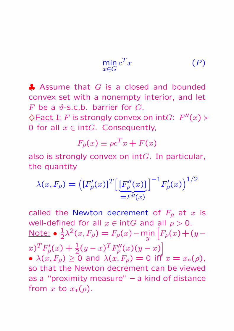
minx∈G
cTx (P )
♣ Assume that G is a closed and boundedconvex set with a nonempty interior, and letF be a ϑ-s.c.b. barrier for G.♦Fact I: F is strongly convex on intG: F ′′(x) Â0 for all x ∈ intG. Consequently,
Fρ(x) ≡ ρcTx + F (x)
also is strongly convex on intG. In particular,the quantity
λ(x, Fρ) =([F ′ρ(x)]T
[[F ′′ρ (x)]︸ ︷︷ ︸=F ′′(x)
]−1F ′ρ(x)
)1/2
called the Newton decrement of Fρ at x iswell-defined for all x ∈ intG and all ρ > 0.Note: • 1
2λ2(x, Fρ) = Fρ(x)−miny
[Fρ(x)+(y−
x)TF ′ρ(x) + 12(y − x)TF ′′ρ (x)(y − x)
]
• λ(x, Fρ) ≥ 0 and λ(x, Fρ) = 0 iff x = x∗(ρ),so that the Newton decrement can be viewedas a “proximity measure” – a kind of distancefrom x to x∗(ρ).

c∗ = minx∈G
cTx (P )
♣ Fact II: Let (P ) be solved via the classicalpenalty scheme implemented as follows:♦The barrier underlying the scheme is a ϑ-s.-c.b. F for G;♦“Closeness” of x and x∗(ρ) is specified bythe relation λ(x, Fρ) ≤ 0.1;
♦The penalty update is ρi+1 =(1 + γ√
ϑ
)ρi,
where γ > 0 is a parameter;♦To update xi into xi+1, we apply to Fρi+1
the Damped Newton method started as xi:
x 7→ x− 1
1 + λ(x, Fρi+1)[F ′′ρi+1
(x)]−1F ′ρi+1(x)
• The method is well-defined, and the num-ber of damped Newton steps in updatingxi 7→ xi+1 depends solely on γ (and is as smallas 1 for γ = 0.1)• One has cTxi − c∗ ≤ 2ϑ
ρi
⇒ With the outlined method, it takes O(√
ϑ)Newton steps to reduce inaccuracy cTx − c∗by absolute constant factor!

♣ Fact III: • Every convex domain G ⊂ Rn
admits O(n)-s.-c.b.• For typical feasible domains arising in Con-vex Programming, one can point out explicit“computable” s.-c.b.’s. For example,♠ Let G be given by m convex quadratic con-straints:
G = x : xTATj Ajx + 2bT
j x + cj︸ ︷︷ ︸gj(x)
≤ 0, 1 ≤ j ≤ m
satisfying the Slater condition. Then the log-arithmic barrier
F (x) = −m∑
j=1
ln(−gj(x))
is m-s.-c.b. for G.♠ Let G be given by Linear Matrix Inequality
G = x : A0 + x1A1 + ... + xnAn︸ ︷︷ ︸A(x):m×m
º 0
satisfying the Slater condition: A(x) Â 0 forsome x. Then the log-det barrier
F (x) = − lnDet(A(x))
is m-s.-c.b. for G.

♣ Consider an LP
minz
cT z : Az − b ≥ 0
(P )
with m × n matrix A, Null(A) = 0, along
with the dual problem
maxy
bTy : ATy = c, y ≥ 0
(D)
and assume that both problems are strictly
feasible:
∃z : Az − b > 0 & ∃y > 0 : ATy = c
Note: Passing from z to “primal slack” x =
Az − b, we can rewrite (P ) as
minx
eTx : x ≥ 0, x ∈ L = ImA− b
(P ′)
where e is a vector satisfying AT e = c, so
that
eTx = eT (Az−b) = (AT e)Tz−const = cT z−const
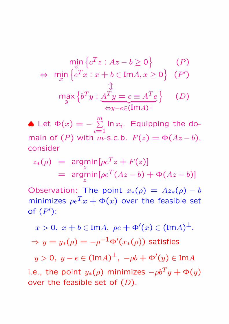
minz
cTz : Az − b ≥ 0
(P )
⇔ minx
eTx : x + b ∈ ImA, x ≥ 0
(P ′)
mmax
y
bTy : ATy = c ≡ AT e︸ ︷︷ ︸
⇔y−e∈(ImA)⊥
(D)
♠ Let Φ(x) = −m∑
i=1lnxi. Equipping the do-
main of (P ) with m-s.c.b. F (z) = Φ(Az− b),
consider
z∗(ρ) = argminz
[ρcT z + F (z)]
= argminz
[ρeT (Az − b) + Φ(Az − b)]
Observation: The point x∗(ρ) = Az∗(ρ) − b
minimizes ρeTx + Φ(x) over the feasible set
of (P ′):
x > 0, x + b ∈ ImA, ρe + Φ′(x) ∈ (ImA)⊥.
⇒ y = y∗(ρ) = −ρ−1Φ′(x∗(ρ)) satisfies
y > 0, y − e ∈ (ImA)⊥, −ρb + Φ′(y) ∈ ImA
i.e., the point y∗(ρ) minimizes −ρbTy + Φ(y)
over the feasible set of (D).

♣ We arrive at a nice symmetric picture:♣ The primal central path x ≡ x∗(ρ) whichminimizes the primal aggregate
ρcTx + Φ(x) [Φ(x) = −∑ilnxi]
over the primal feasible set is given by
x > 0, x + b ∈ ImA, ρc + Φ′(x) ∈ (ImA)⊥
♣ The dual central path y ≡ y∗(ρ) which min-imizes the dual aggregate
−ρbTy + Φ(y) [Φ(y) = −∑iln yi]
over the dual feasible set is given by
y > 0, y − e ∈ (ImA)⊥,−ρb + Φ′(y) ∈ ImA
♣ The paths are linked by
y = −ρ−1Φ′(x) ⇔ x = −Φ′(y∗(ρ)) ⇔ xiyi =1
ρ∀i.
⇒ DualityGap(x, y) = xTy = [cTx−Opt(P )]+[Opt(D)− bTy]
on the path is equal to mρ−1.
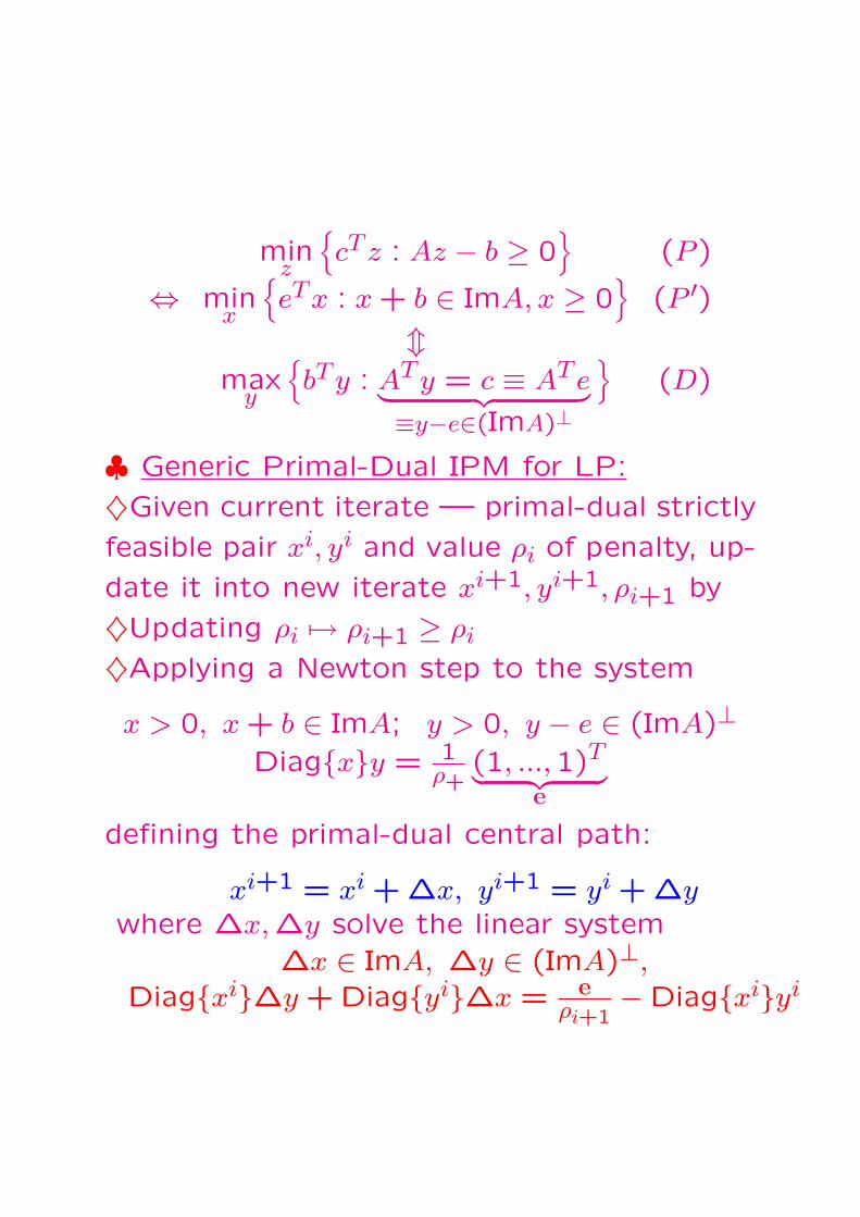
minz
cTz : Az − b ≥ 0
(P )
⇔ minx
eTx : x + b ∈ ImA, x ≥ 0
(P ′)
mmax
y
bTy : ATy = c ≡ AT e︸ ︷︷ ︸
≡y−e∈(ImA)⊥
(D)
♣ Generic Primal-Dual IPM for LP:
♦Given current iterate — primal-dual strictly
feasible pair xi, yi and value ρi of penalty, up-
date it into new iterate xi+1, yi+1, ρi+1 by
♦Updating ρi 7→ ρi+1 ≥ ρi
♦Applying a Newton step to the system
x > 0, x + b ∈ ImA; y > 0, y − e ∈ (ImA)⊥Diagxy = 1
ρ+(1, ...,1)T︸ ︷︷ ︸
e
defining the primal-dual central path:
xi+1 = xi + ∆x, yi+1 = yi + ∆ywhere ∆x,∆y solve the linear system
∆x ∈ ImA, ∆y ∈ (ImA)⊥,
Diagxi∆y + Diagyi∆x = eρi+1
−Diagxiyi
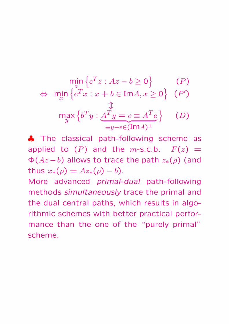
minz
cTz : Az − b ≥ 0
(P )
⇔ minx
eTx : x + b ∈ ImA, x ≥ 0
(P ′)
mmax
y
bTy : ATy = c ≡ AT e︸ ︷︷ ︸
≡y−e∈(ImA)⊥
(D)
♣ The classical path-following scheme as
applied to (P ) and the m-s.c.b. F (z) =
Φ(Az− b) allows to trace the path z∗(ρ) (and
thus x∗(ρ) = Az∗(ρ)− b).
More advanced primal-dual path-following
methods simultaneously trace the primal and
the dual central paths, which results in algo-
rithmic schemes with better practical perfor-
mance than the one of the “purely primal”
scheme.
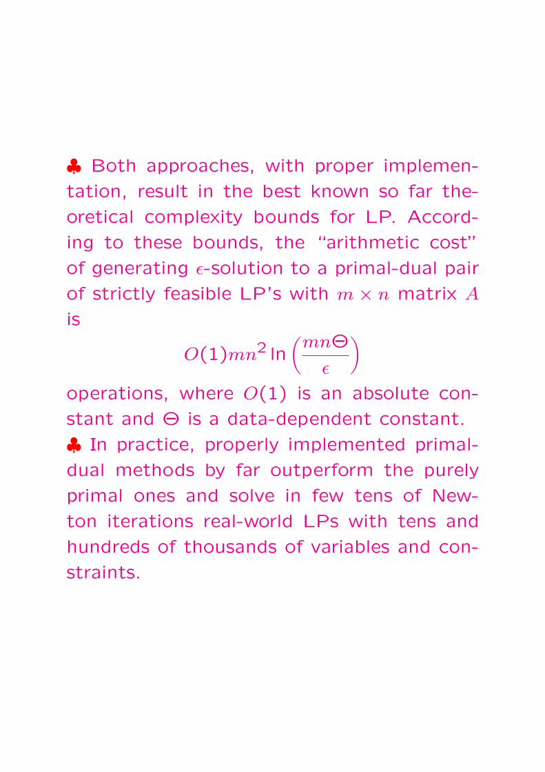
♣ Both approaches, with proper implemen-
tation, result in the best known so far the-
oretical complexity bounds for LP. Accord-
ing to these bounds, the “arithmetic cost”
of generating ε-solution to a primal-dual pair
of strictly feasible LP’s with m× n matrix A
is
O(1)mn2 ln(
mnΘ
ε
)
operations, where O(1) is an absolute con-
stant and Θ is a data-dependent constant.
♣ In practice, properly implemented primal-
dual methods by far outperform the purely
primal ones and solve in few tens of New-
ton iterations real-world LPs with tens and
hundreds of thousands of variables and con-
straints.
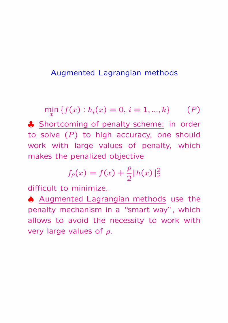
Augmented Lagrangian methods
minxf(x) : hi(x) = 0, i = 1, ..., k (P )
♣ Shortcoming of penalty scheme: in order
to solve (P ) to high accuracy, one should
work with large values of penalty, which
makes the penalized objective
fρ(x) = f(x) +ρ
2‖h(x)‖22
difficult to minimize.
♠ Augmented Lagrangian methods use the
penalty mechanism in a “smart way”, which
allows to avoid the necessity to work with
very large values of ρ.
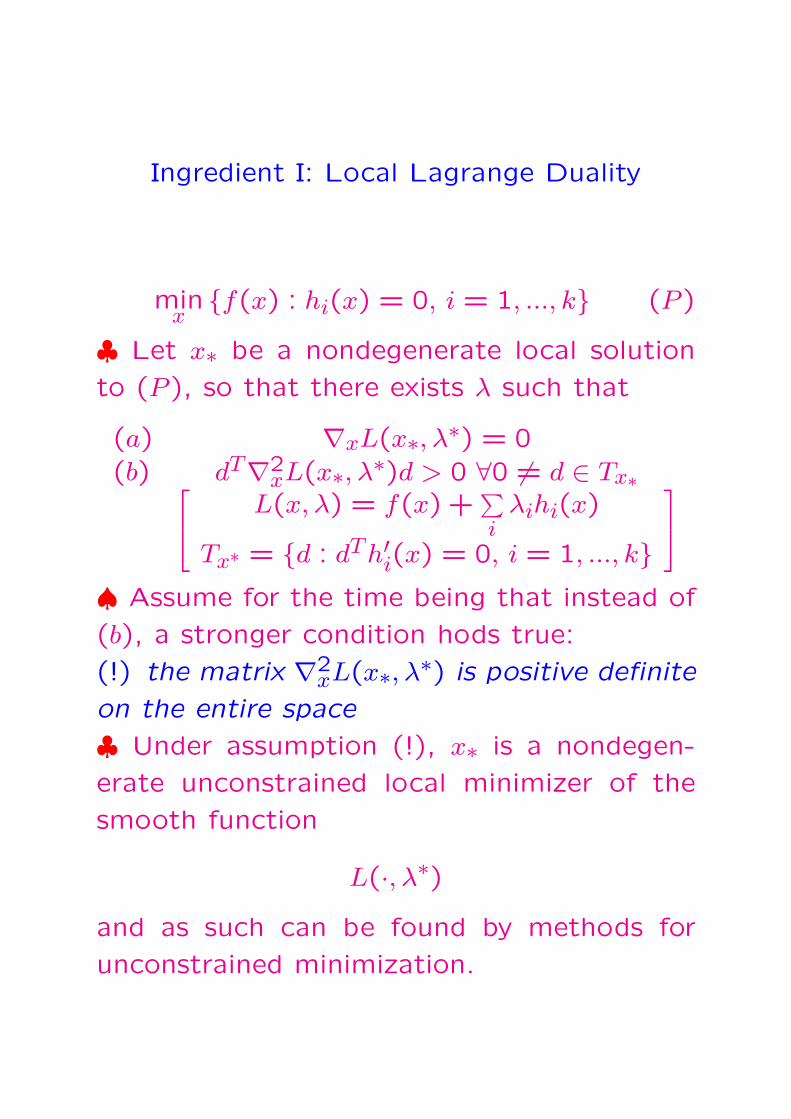
Ingredient I: Local Lagrange Duality
minxf(x) : hi(x) = 0, i = 1, ..., k (P )
♣ Let x∗ be a nondegenerate local solution
to (P ), so that there exists λ such that
(a) ∇xL(x∗, λ∗) = 0(b) dT∇2
xL(x∗, λ∗)d > 0 ∀0 6= d ∈ Tx∗ L(x, λ) = f(x) +
∑i
λihi(x)
Tx∗ = d : dTh′i(x) = 0, i = 1, ..., k
♠ Assume for the time being that instead of
(b), a stronger condition hods true:
(!) the matrix ∇2xL(x∗, λ∗) is positive definite
on the entire space
♣ Under assumption (!), x∗ is a nondegen-
erate unconstrained local minimizer of the
smooth function
L(·, λ∗)and as such can be found by methods for
unconstrained minimization.
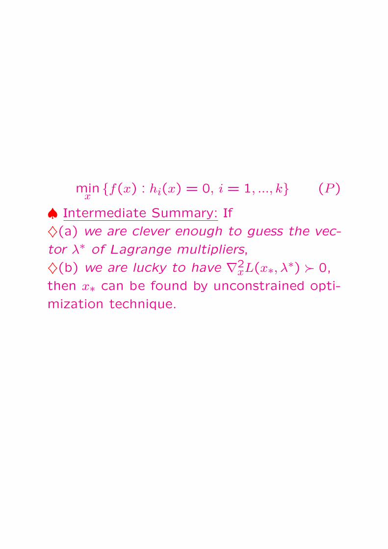
minxf(x) : hi(x) = 0, i = 1, ..., k (P )
♠ Intermediate Summary: If
♦(a) we are clever enough to guess the vec-
tor λ∗ of Lagrange multipliers,
♦(b) we are lucky to have ∇2xL(x∗, λ∗) Â 0,
then x∗ can be found by unconstrained opti-
mization technique.

♠ How to become smart when being lucky: Lo-cal Lagrange Duality.Situation: x∗ is a nondegenerate local solu-tion to
minxf(x) : hi(x) = 0, i = 1, ..., k (P )
and we are lucky:
∃λ∗ : ∇xL(x∗, λ∗) = 0, ∇2xL(x∗, λ∗) Â 0 (!)
Fact: Under assumption (!), there exist con-vex neighbourhood V of x∗ and convex neigh-bourhood Λ of λ∗ such that(i) For every λ ∈ Λ, function L(x, λ) isstrongly convex in x ∈ V and possessesuniquely defined critical point x∗(λ) in V
which is continuously differentiable in λ ∈ Λ.x∗(λ) is a nondegenerate local minimizer ofL(·, λ);(ii) The function
L(λ) = L(x∗(λ), λ) = minx∈V
L(x, λ)
is C2-smooth and concave in Λ,
L′(λ) = h(x∗(λ)),
and λ∗ is a nondegenerate maximizer of L(λ)on Λ.
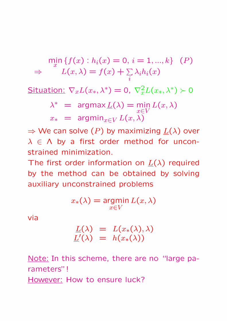
minxf(x) : hi(x) = 0, i = 1, ..., k (P )
⇒ L(x, λ) = f(x) +∑i
λihi(x)
Situation: ∇xL(x∗, λ∗) = 0, ∇2xL(x∗, λ∗) Â 0
λ∗ = argmaxL(λ) = minx∈V
L(x, λ)
x∗ = argminx∈V L(x, λ)
⇒ We can solve (P ) by maximizing L(λ) over
λ ∈ Λ by a first order method for uncon-
strained minimization.
The first order information on L(λ) required
by the method can be obtained by solving
auxiliary unconstrained problems
x∗(λ) = argminx∈V
L(x, λ)
via
L(λ) = L(x∗(λ), λ)L′(λ) = h(x∗(λ))
Note: In this scheme, there are no “large pa-
rameters”!
However: How to ensure luck?
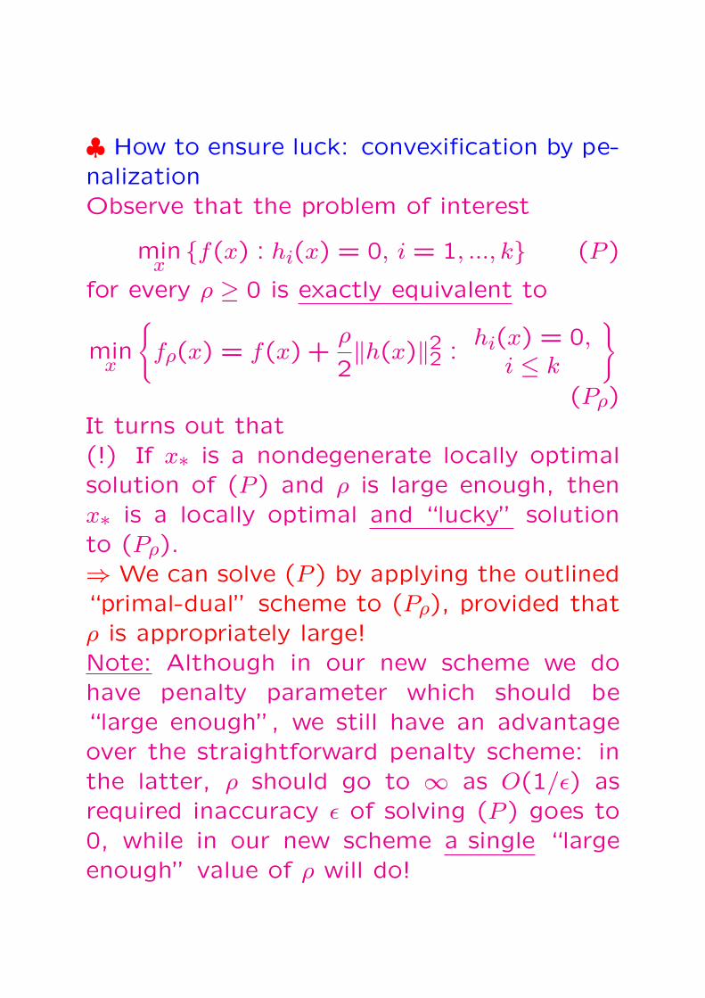
♣ How to ensure luck: convexification by pe-nalizationObserve that the problem of interest
minxf(x) : hi(x) = 0, i = 1, ..., k (P )
for every ρ ≥ 0 is exactly equivalent to
minx
fρ(x) = f(x) +
ρ
2‖h(x)‖22 :
hi(x) = 0,i ≤ k
(Pρ)It turns out that(!) If x∗ is a nondegenerate locally optimalsolution of (P ) and ρ is large enough, thenx∗ is a locally optimal and “lucky” solutionto (Pρ).⇒ We can solve (P ) by applying the outlined“primal-dual” scheme to (Pρ), provided thatρ is appropriately large!Note: Although in our new scheme we dohave penalty parameter which should be“large enough”, we still have an advantageover the straightforward penalty scheme: inthe latter, ρ should go to ∞ as O(1/ε) asrequired inaccuracy ε of solving (P ) goes to0, while in our new scheme a single “largeenough” value of ρ will do!

minxf(x) : hi(x) = 0, i = 1, ..., k (P )
mmin
x
fρ(x) = f(x) + ρ
2‖h(x)‖22 :hi(x) = 0,
i ≤ k
(Pρ)
Justifying the claim: Let
Lρ(x, λ) = f(x) +ρ
2‖h(x)‖22 +
∑
i
λihi(x)
be the Lagrange function of (Pρ); the La-
grange function of (P ) is then Lo(x, λ). Given
nondegenerate locally optimal solution x∗ to
(P ), let λ∗ be the corresponding Lagrange
multipliers. We have
∇xLρ(x∗, λ∗) = ∇xL0(x∗, λ∗) + ρ∑i
hi(x∗)h′i(x∗)
= ∇xL0(x∗, λ∗)= 0∇2
xLρ(x∗λ∗) = ∇2xL(x∗, λ∗) + ρ
∑i
hi(x∗)h′′i (x∗)
+ρ∑i
h′i(x∗)[h′i(x∗)]T
= ∇2xL0(x∗, ρ∗) + ρHTH,
H =
[h′1(x∗)]T· · ·
[h′k(x∗)]T
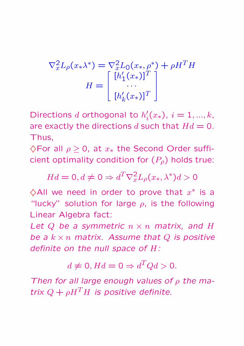
∇2xLρ(x∗λ∗) = ∇2
xL0(x∗, ρ∗) + ρHTH
H =
[h′1(x∗)]T· · ·
[h′k(x∗)]T
Directions d orthogonal to h′i(x∗), i = 1, ..., k,
are exactly the directions d such that Hd = 0.
Thus,
♦For all ρ ≥ 0, at x∗ the Second Order suffi-
cient optimality condition for (Pρ) holds true:
Hd = 0, d 6= 0 ⇒ dT∇2xLρ(x∗, λ∗)d > 0
♦All we need in order to prove that x∗ is a
“lucky” solution for large ρ, is the following
Linear Algebra fact:
Let Q be a symmetric n × n matrix, and H
be a k× n matrix. Assume that Q is positive
definite on the null space of H:
d 6= 0, Hd = 0 ⇒ dTQd > 0.
Then for all large enough values of ρ the ma-
trix Q + ρHTH is positive definite.

Let Q be a symmetric n × n matrix, and Hbe a k× n matrix. Assume that Q is positivedefinite on the null space of H:
d 6= 0, Hd = 0 ⇒ dTQd > 0.
Then for all large enough values of ρ the ma-trix Q + ρHTH is positive definite.Proof: Assume, on the contrary, that thereexists a sequence ρi →∞ and di, ‖di‖2 = 1:
dTi [Q + ρiH
TH]di ≤ 0 ∀i.Passing to a subsequence, we may assumethat di → d, i → ∞. Let di = hi + h⊥i bethe decomposition of di into the sum of itsprojections onto Null(H) and [Null(H)]⊥, andsimilarly d = h + h⊥. Then
dTi HTHdi = ‖Hdi‖22 = ‖Hh⊥i ‖22 → ‖Hh⊥‖22 ⇒
0 ≥ dTi [Q + ρiH
TH]di = dTi Qdi︸ ︷︷ ︸→dT Qd
+ρi ‖Hh⊥i ‖22︸ ︷︷ ︸→‖Hh⊥‖22
(∗)
If h⊥ 6= 0, then ‖Hh⊥‖2 > 0, and the righthand side in (∗) tends to +∞ as i → ∞,which is impossible. Thus, h⊥ = 0. But then0 6= d ∈ Null(H) and therefore dTQd > 0, sothat the right hand side in (∗) is positive forlarge i, which again is impossible.
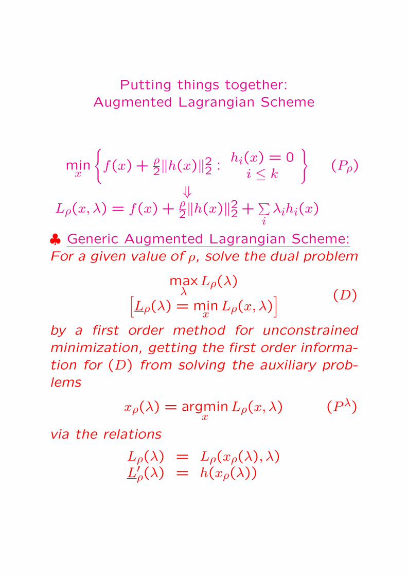
Putting things together:Augmented Lagrangian Scheme
minx
f(x) + ρ
2‖h(x)‖22 :hi(x) = 0
i ≤ k
(Pρ)
⇓Lρ(x, λ) = f(x) + ρ
2‖h(x)‖22 +∑i
λihi(x)
♣ Generic Augmented Lagrangian Scheme:For a given value of ρ, solve the dual problem
maxλ
Lρ(λ)[Lρ(λ) = min
xLρ(x, λ)
] (D)
by a first order method for unconstrainedminimization, getting the first order informa-tion for (D) from solving the auxiliary prob-lems
xρ(λ) = argminx
Lρ(x, λ) (Pλ)
via the relations
Lρ(λ) = Lρ(xρ(λ), λ)L′ρ(λ) = h(xρ(λ))
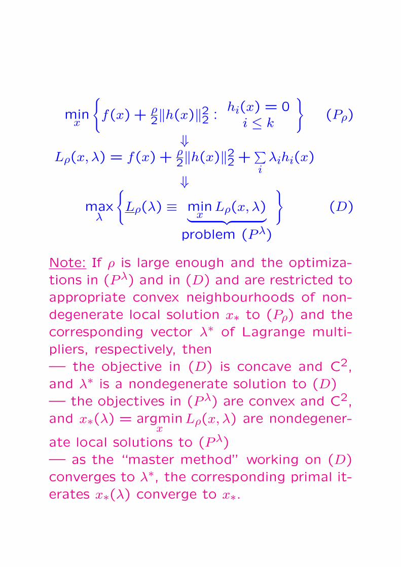
minx
f(x) + ρ
2‖h(x)‖22 :hi(x) = 0
i ≤ k
(Pρ)
⇓Lρ(x, λ) = f(x) + ρ
2‖h(x)‖22 +∑i
λihi(x)
⇓max
λ
Lρ(λ) ≡ min
xLρ(x, λ)
︸ ︷︷ ︸problem (Pλ)
(D)
Note: If ρ is large enough and the optimiza-tions in (Pλ) and in (D) and are restricted toappropriate convex neighbourhoods of non-degenerate local solution x∗ to (Pρ) and thecorresponding vector λ∗ of Lagrange multi-pliers, respectively, then— the objective in (D) is concave and C2,and λ∗ is a nondegenerate solution to (D)— the objectives in (Pλ) are convex and C2,and x∗(λ) = argmin
xLρ(x, λ) are nondegener-
ate local solutions to (Pλ)— as the “master method” working on (D)converges to λ∗, the corresponding primal it-erates x∗(λ) converge to x∗.
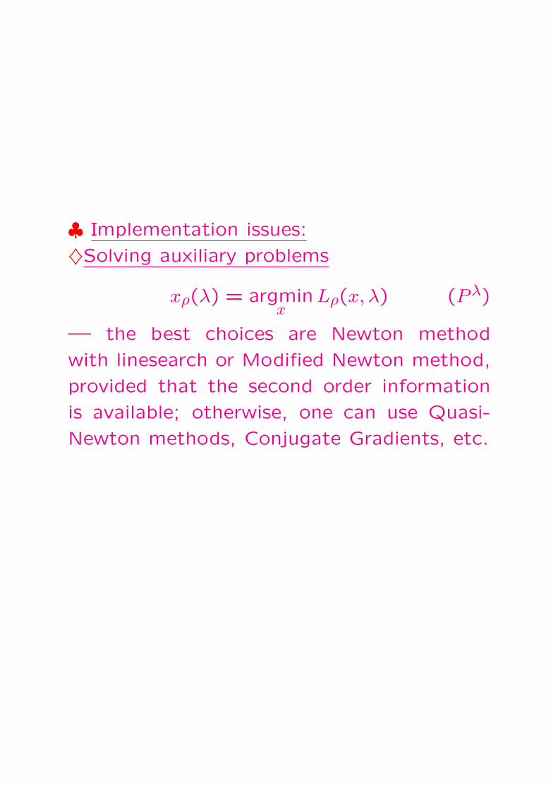
♣ Implementation issues:
♦Solving auxiliary problems
xρ(λ) = argminx
Lρ(x, λ) (Pλ)
— the best choices are Newton method
with linesearch or Modified Newton method,
provided that the second order information
is available; otherwise, one can use Quasi-
Newton methods, Conjugate Gradients, etc.
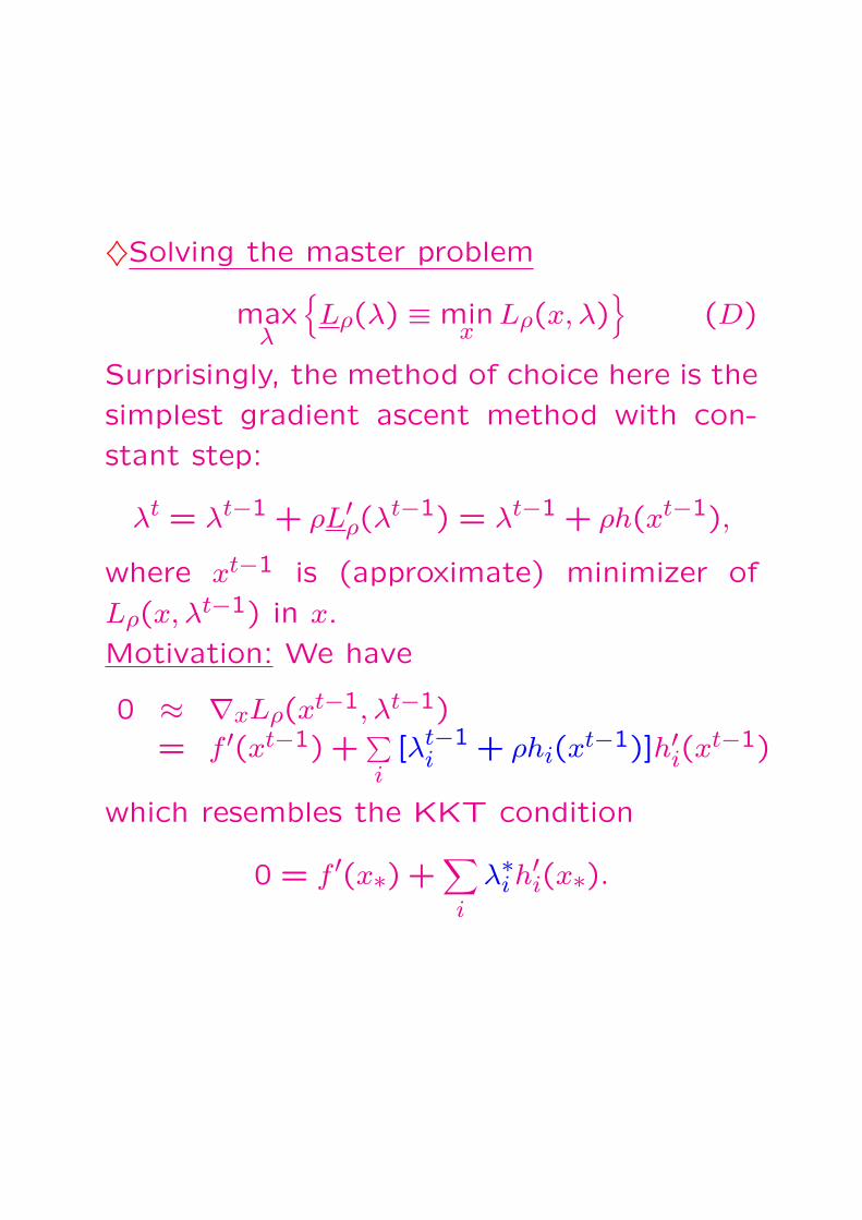
♦Solving the master problem
maxλ
Lρ(λ) ≡ min
xLρ(x, λ)
(D)
Surprisingly, the method of choice here is the
simplest gradient ascent method with con-
stant step:
λt = λt−1 + ρL′ρ(λt−1) = λt−1 + ρh(xt−1),
where xt−1 is (approximate) minimizer of
Lρ(x, λt−1) in x.
Motivation: We have
0 ≈ ∇xLρ(xt−1, λt−1)
= f ′(xt−1) +∑i[λt−1
i + ρhi(xt−1)]h′i(xt−1)
which resembles the KKT condition
0 = f ′(x∗) +∑
i
λ∗i h′i(x∗).
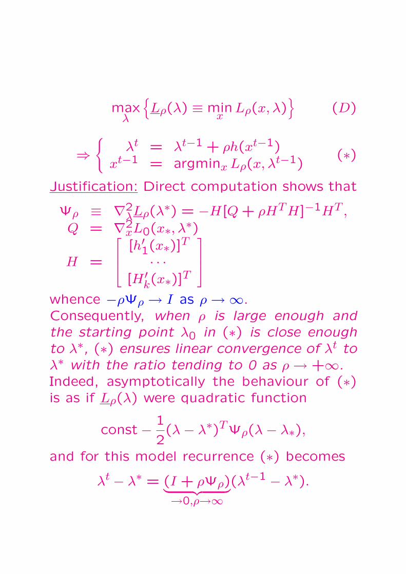
maxλ
Lρ(λ) ≡ min
xLρ(x, λ)
(D)
⇒
λt = λt−1 + ρh(xt−1)xt−1 = argminx Lρ(x, λt−1)
(∗)
Justification: Direct computation shows that
Ψρ ≡ ∇2λLρ(λ∗) = −H[Q + ρHTH]−1HT ,
Q = ∇2xL0(x∗, λ∗)
H =
[h′1(x∗)]T· · ·
[H ′k(x∗)]
T
whence −ρΨρ → I as ρ →∞.Consequently, when ρ is large enough andthe starting point λ0 in (∗) is close enoughto λ∗, (∗) ensures linear convergence of λt toλ∗ with the ratio tending to 0 as ρ → +∞.Indeed, asymptotically the behaviour of (∗)is as if Lρ(λ) were quadratic function
const− 1
2(λ− λ∗)TΨρ(λ− λ∗),
and for this model recurrence (∗) becomes
λt − λ∗ = (I + ρΨρ)︸ ︷︷ ︸→0,ρ→∞
(λt−1 − λ∗).

♣ Adjusting penalty parameter:
⇒
λt = λt−1 + ρh(xt−1)xt−1 = argminx Lρ(x, λt−1)
(∗)
When ρ is “large enough”, so that (∗) con-
verges linearly with reasonable convergence
ratio, ‖L′ρ(λt)‖2 = ‖h(xt)‖2 should go to 0
linearly with essentially the same ratio.
⇒ We can use progress in ‖h(·)‖2 to con-
trol ρ, e.g., as follows: when ‖h(xt)‖2 ≤0.25‖h(xt−1)‖2, we keep the current value
of ρ intact, otherwise we increase penalty
by factor 10 and recompute xt with the new
value of ρ.
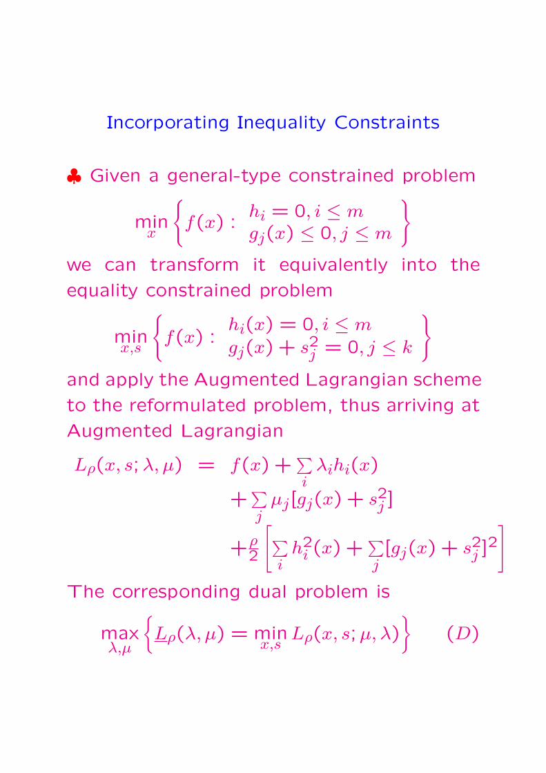
Incorporating Inequality Constraints
♣ Given a general-type constrained problem
minx
f(x) :
hi = 0, i ≤ mgj(x) ≤ 0, j ≤ m
we can transform it equivalently into the
equality constrained problem
minx,s
f(x) :
hi(x) = 0, i ≤ m
gj(x) + s2j = 0, j ≤ k
and apply the Augmented Lagrangian scheme
to the reformulated problem, thus arriving at
Augmented Lagrangian
Lρ(x, s;λ, µ) = f(x) +∑i
λihi(x)
+∑j
µj[gj(x) + s2j ]
+ρ2
[∑i
h2i (x) +
∑j[gj(x) + s2j ]
2
]
The corresponding dual problem is
maxλ,µ
Lρ(λ, µ) = min
x,sLρ(x, s;µ, λ)
(D)

Lρ(x, s;λ, µ) = f(x) +∑i
λihi(x)
+∑j
µj[gj(x) + s2j ]
+ρ2
[∑i
h2i (x) +
∑j[gj(x) + s2j ]
2
]
⇓maxλ,µ
Lρ(λ, µ) ≡ min
x,sLρ(x, s;µ, λ)
We can carry out the minimization in s ana-
lytically, arriving at
Lρ(λ, µ) = minx
f(x) + ρ
2
k∑j=1
(gj(x) +
µjρ
)2
+
+m∑
i=1λihi(x) + ρ
2
m∑i=1
hi(x)2
−k∑
j=1
µ2j
2ρ
where a+ = max[0, a].
⇒ The auxiliary problems arising in the Aug-
mented Lagrangian Scheme are problems in
the initial design variables!

minx
f(x) :
hi(x) = 0, i ≤ kgj(x) ≤ 0, j ≤ m
(P )
⇓minx,s
f(x) :
hi(x) = 0, i ≤ k
gj(x) + s2j = 0, j ≤ m
(P ′)
♣ Theoretical analysis of Augmented La-
grangian scheme for problems with equality
constraints was based on assumption that we
are trying to approximate nondegenerate lo-
cal solution. Is it true that when applying
reducing the inequality constrained problem
to an equality constrained one, we preserve
nondegeneracy of the local solution?
Yes!
Theorem. Let x∗ be a nondegenerate local
solution to (P ). Then the point
(x∗, s∗) : s∗j =√−gj(x∗), j = 1, ..., m
is a nondegenerate local solution to (P ′).
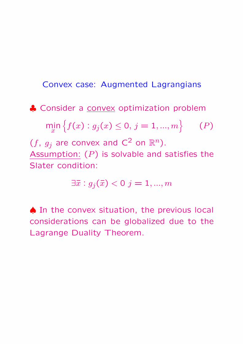
Convex case: Augmented Lagrangians
♣ Consider a convex optimization problem
minx
f(x) : gj(x) ≤ 0, j = 1, ..., m
(P )
(f , gj are convex and C2 on Rn).
Assumption: (P ) is solvable and satisfies the
Slater condition:
∃x : gj(x) < 0 j = 1, ..., m
♠ In the convex situation, the previous local
considerations can be globalized due to the
Lagrange Duality Theorem.
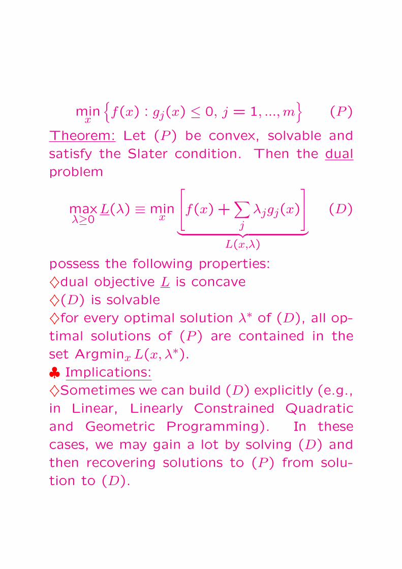
minx
f(x) : gj(x) ≤ 0, j = 1, ..., m
(P )
Theorem: Let (P ) be convex, solvable and
satisfy the Slater condition. Then the dual
problem
maxλ≥0
L(λ) ≡ minx
f(x) +
∑
j
λjgj(x)
︸ ︷︷ ︸L(x,λ)
(D)
possess the following properties:
♦dual objective L is concave
♦(D) is solvable
♦for every optimal solution λ∗ of (D), all op-
timal solutions of (P ) are contained in the
set Argminx L(x, λ∗).♣ Implications:
♦Sometimes we can build (D) explicitly (e.g.,
in Linear, Linearly Constrained Quadratic
and Geometric Programming). In these
cases, we may gain a lot by solving (D) and
then recovering solutions to (P ) from solu-
tion to (D).

minx
f(x) : gj(x) ≤ 0, j = 1, ..., m
(P )
⇓
maxλ≥0
L(λ) ≡ minx
f(x) +
∑
j
λjgj(x)
︸ ︷︷ ︸L(x,λ)
(D)
♦In the general case one can solve (D) nu-merically by a first order method, thus re-ducing a problem with general convex con-straints to one with simple linear constraints.To solve (D) numerically, we should be ableto compute the first order information for L.This can be done via solving the auxiliaryproblems
x∗ = x∗(λ) = minx
L(x, λ) (Pλ)
due to
L(λ) = L(x∗(λ), λ)L′(λ) = g(x∗(λ))
Note: (Pλ) is a convex unconstrained pro-gram with smooth objective!
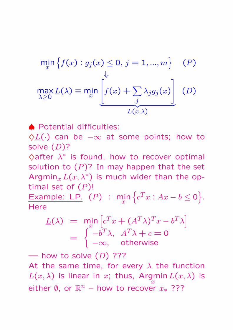
minx
f(x) : gj(x) ≤ 0, j = 1, ..., m
(P )
⇓
maxλ≥0
L(λ) ≡ minx
f(x) +
∑
j
λjgj(x)
︸ ︷︷ ︸L(x,λ)
(D)
♠ Potential difficulties:♦L(·) can be −∞ at some points; how tosolve (D)?♦after λ∗ is found, how to recover optimalsolution to (P )? In may happen that the setArgminx L(x, λ∗) is much wider than the op-timal set of (P )!Example: LP. (P ) : min
x
cTx : Ax− b ≤ 0
.
Here
L(λ) = minx
[cTx + (ATλ)Tx− bTλ
]
=
−bTλ, ATλ + c = 0−∞, otherwise
— how to solve (D) ???At the same time, for every λ the functionL(x, λ) is linear in x; thus, Argmin
xL(x, λ) is
either ∅, or Rn – how to recover x∗ ???

♠Observation: Both outlined difficulties comefrom possible non-existence/non-uniquenessof solutions to the auxiliary problems
minx
L(x, λ) ≡ minx
[f(x) +∑
j
λjgj(x)] (Pλ)
Indeed, if solution x∗(λ) to (Pλ) exists and isunique and continuous in λ on certain set Λ,then L(λ) is finite and continuously differen-tiable on Λ due to
L(λ) = L(x∗(λ), λ)L′(λ) = g(x∗(λ))
Besides this, if λ∗ ∈ Λ, then there is no prob-lem with recovering optimal solution to (P )from λ∗.Example: Assume that the function
r(x) = f(x) +k∑
j=1
gj(x)
is locally strongly convex (r′′(x) Â 0 ∀x) andis such that
r(x)/‖x‖2 →∞, ‖x‖2 →∞.
Then x∗(λ) exists, is unique and is continuousin λ on the set Λ = λ > 0.

♣ In Augmented Lagrangian scheme, we en-
sure local strong convexity of
r(·) = f(x) + sum of constraints
by passing from the original problem
minx
f(x) : gj(x) ≤ 0, j = 1, ..., m
(P )
to the equivalent problem
minx
f(x) : θj(gj(x)) ≤ 0, j = 1, ..., m
(P ′)
where θj(·) are increasing strongly convex
smooth functions satisfying the normaliza-
tion
θj(0) = 0, θ′j(0) = 1.
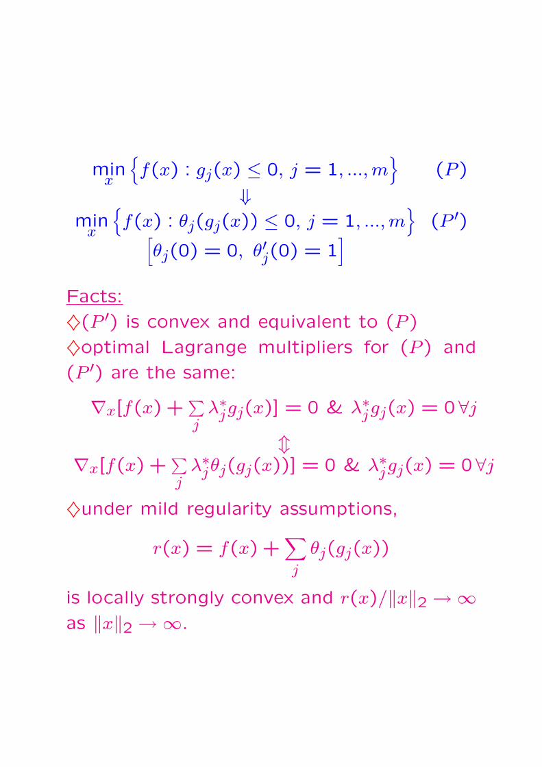
minx
f(x) : gj(x) ≤ 0, j = 1, ..., m
(P )
⇓min
x
f(x) : θj(gj(x)) ≤ 0, j = 1, ..., m
(P ′)[
θj(0) = 0, θ′j(0) = 1]
Facts:
♦(P ′) is convex and equivalent to (P )
♦optimal Lagrange multipliers for (P ) and
(P ′) are the same:
∇x[f(x) +∑j
λ∗jgj(x)] = 0 & λ∗jgj(x) = 0∀jm
∇x[f(x) +∑j
λ∗jθj(gj(x))] = 0 & λ∗jgj(x) = 0∀j
♦under mild regularity assumptions,
r(x) = f(x) +∑
j
θj(gj(x))
is locally strongly convex and r(x)/‖x‖2 →∞as ‖x‖2 →∞.
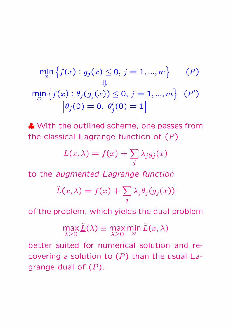
minx
f(x) : gj(x) ≤ 0, j = 1, ..., m
(P )
⇓min
x
f(x) : θj(gj(x)) ≤ 0, j = 1, ..., m
(P ′)[
θj(0) = 0, θ′j(0) = 1]
♣ With the outlined scheme, one passes from
the classical Lagrange function of (P )
L(x, λ) = f(x) +∑
j
λjgj(x)
to the augmented Lagrange function
L(x, λ) = f(x) +∑
j
λjθj(gj(x))
of the problem, which yields the dual problem
maxλ≥0
L(λ) ≡ maxλ≥0
minx
L(x, λ)
better suited for numerical solution and re-
covering a solution to (P ) than the usual La-
grange dual of (P ).
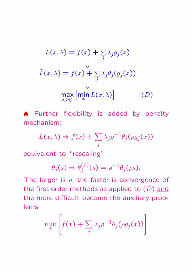
L(x, λ) = f(x) +∑j
λjgj(x)
⇓L(x, λ) = f(x) +
∑j
λjθj(gj(x))
⇓maxλ≥0
[min
xL(x, λ)
](D)
♠ Further flexibility is added by penalty
mechanism:
L(x, λ) ⇒ f(x) +∑
j
λjρ−1θj(ρgj(x))
equivalent to “rescaling”
θj(s) ⇒ θ(ρ)j (s) = ρ−1θj(ρs).
The larger is ρ, the faster is convergence of
the first order methods as applied to (D) and
the more difficult become the auxiliary prob-
lems
minx
f(x) +
∑
j
λjρ−1θj(ρgj(x))
Sequential Quadratic Programming
♣ SQP is thought of to be the most effi-
cient technique for solving general-type opti-
mization problems with smooth objective and
constraints.
♣ SQP methods directly solve the KKT sys-
tem of the problem by a Newton-type itera-
tive process.
♣ Consider an equality constrained problem
minx
f(x) : h(x) = (h1(x), ..., hk(x))
T = 0
(P )
⇒ L(x, λ) = f(x) + hT (x)λ
The KKT system of the problem is
∇xL(x, λ) ≡ f ′(x) + [h′(x)]Tλ = 0∇λL(x, λ) ≡ h(x) = 0
(KKT)
Every locally optimal solution x∗ of (P ) which
is regular (that is, the gradients h′i(x∗)ki=1are linearly independent) can be extended
by properly chosen λ = λ∗ to a solution of
(KKT).
♠ (KKT) is a system of nonlinear equations
with n + k equations and n + k unknowns.
We can try to solve this system by Newton
method.
Newton method for solving nonlinear
systems of equations
♣ To solve a system of N nonlinear equations
with N unknowns
P (u) ≡ (p1(u), ..., pN(u))T = 0,
with C1 real-valued functions pi, we act as
follows:
Given current iterate u, we linearize the sys-
tem at the iterate, thus arriving at the lin-
earized system
P (u) + P ′(u)(u− u)
≡
p1(u) + [p′1(u)]T (u− u)...
pN(u) + [p′N(u)]T (u− u)
= 0.
Assuming the N×N matrix P ′(u) nonsingular,
we solve the linearized system, thus getting
the new iterate
u+ = u−[P ′(u)]−1P (u)︸ ︷︷ ︸Newton
displacement
;

u 7→ u+ = u− [P ′(u)]−1P (u) (N)
Note: The Basic Newton method for uncon-
strained minimization is nothing but the out-
lined process as applied to the Fermat equa-
tion
P (x) ≡ ∇f(x) = 0.
♣ Same as in the optimization case, the New-
ton method possesses fast local convergence:
Theorem. Let u∗ ∈ RN be a solution to the
square system of nonlinear equations
P (u) = 0
with components of P being C1 in a neigh-
bourhood of u∗. Assuming that u∗ is nonde-
generate (i.e., Det(P ′(u∗)) 6= 0), the Newton
method (N), started close enough to u∗, con-
verges to u∗ superlinearly.
If, in addition, the components of P are C2
in a neighbourhood of u∗, then the above
convergence is quadratic.
♣ Applying the outlined scheme to the KKT
system
∇xL(x, λ) ≡ f ′(x) + [h′(x)]Tλ = 0∇λL(x, λ) ≡ h(x) = 0
(KKT)
we should answer first of all the following
crucial question:
(?) When a KKT point (x∗, λ∗) is a nonde-
generate solution to (KKT)?
Let us set
P (x, λ) = ∇x,λL(x, λ)
=
[∇xL(x, λ) ≡ f ′(x) + [h′(x)]Tλ
∇λL(x, λ) ≡ h(x)
]
Note that
P ′(x, λ) =
[∇2
xL(x, λ) [h′(x)]Th′(x) 0
]
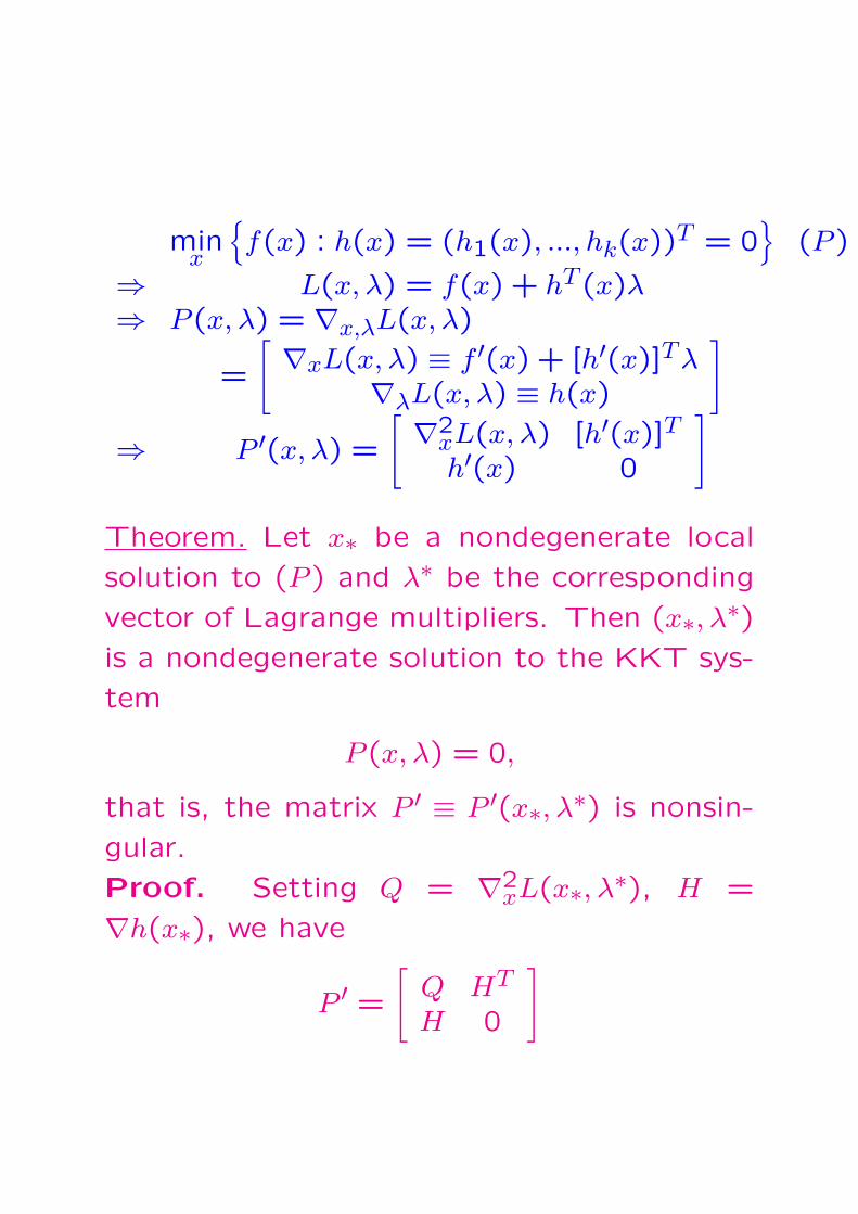
minx
f(x) : h(x) = (h1(x), ..., hk(x))
T = 0
(P )
⇒ L(x, λ) = f(x) + hT (x)λ⇒ P (x, λ) = ∇x,λL(x, λ)
=
[∇xL(x, λ) ≡ f ′(x) + [h′(x)]Tλ
∇λL(x, λ) ≡ h(x)
]
⇒ P ′(x, λ) =
[∇2
xL(x, λ) [h′(x)]Th′(x) 0
]
Theorem. Let x∗ be a nondegenerate local
solution to (P ) and λ∗ be the corresponding
vector of Lagrange multipliers. Then (x∗, λ∗)is a nondegenerate solution to the KKT sys-
tem
P (x, λ) = 0,
that is, the matrix P ′ ≡ P ′(x∗, λ∗) is nonsin-
gular.
Proof. Setting Q = ∇2xL(x∗, λ∗), H =
∇h(x∗), we have
P ′ =[
Q HT
H 0
]

Q = ∇2xL(x∗, λ∗), H = ∇h(x∗),
P ′ =[
Q HT
H 0
]
We know that d 6= 0, Hd = 0 ⇒ dTQd > 0 and
that the rows of H are linearly independent.
We should prove that if
0 = P ′[
dg
]≡
[Qd + HTg
Hd
],
then d = 0, g = 0. We have Hd = 0 and
0 = Qd + HTg ⇒ dTQd + (Hd)Tg = dTQd,
which, as we know, is possible iff d = 0. We
now have HTg = Qd + HTg = 0; since the
rows of H are linearly independent, it follows
that g = 0.
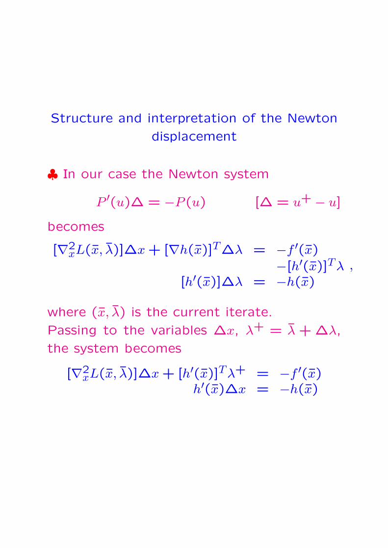
Structure and interpretation of the Newton
displacement
♣ In our case the Newton system
P ′(u)∆ = −P (u) [∆ = u+ − u]
becomes
[∇2xL(x, λ)]∆x + [∇h(x)]T∆λ = −f ′(x)
−[h′(x)]Tλ[h′(x)]∆λ = −h(x)
,
where (x, λ) is the current iterate.
Passing to the variables ∆x, λ+ = λ + ∆λ,
the system becomes
[∇2xL(x, λ)]∆x + [h′(x)]Tλ+ = −f ′(x)
h′(x)∆x = −h(x)
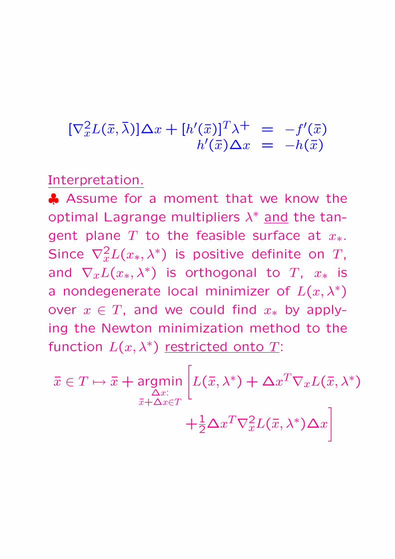
[∇2xL(x, λ)]∆x + [h′(x)]Tλ+ = −f ′(x)
h′(x)∆x = −h(x)
Interpretation.
♣ Assume for a moment that we know the
optimal Lagrange multipliers λ∗ and the tan-
gent plane T to the feasible surface at x∗.Since ∇2
xL(x∗, λ∗) is positive definite on T ,
and ∇xL(x∗, λ∗) is orthogonal to T , x∗ is
a nondegenerate local minimizer of L(x, λ∗)over x ∈ T , and we could find x∗ by apply-
ing the Newton minimization method to the
function L(x, λ∗) restricted onto T :
x ∈ T 7→ x + argmin∆x:
x+∆x∈T
[L(x, λ∗) + ∆xT∇xL(x, λ∗)
+12∆xT∇2
xL(x, λ∗)∆x
]
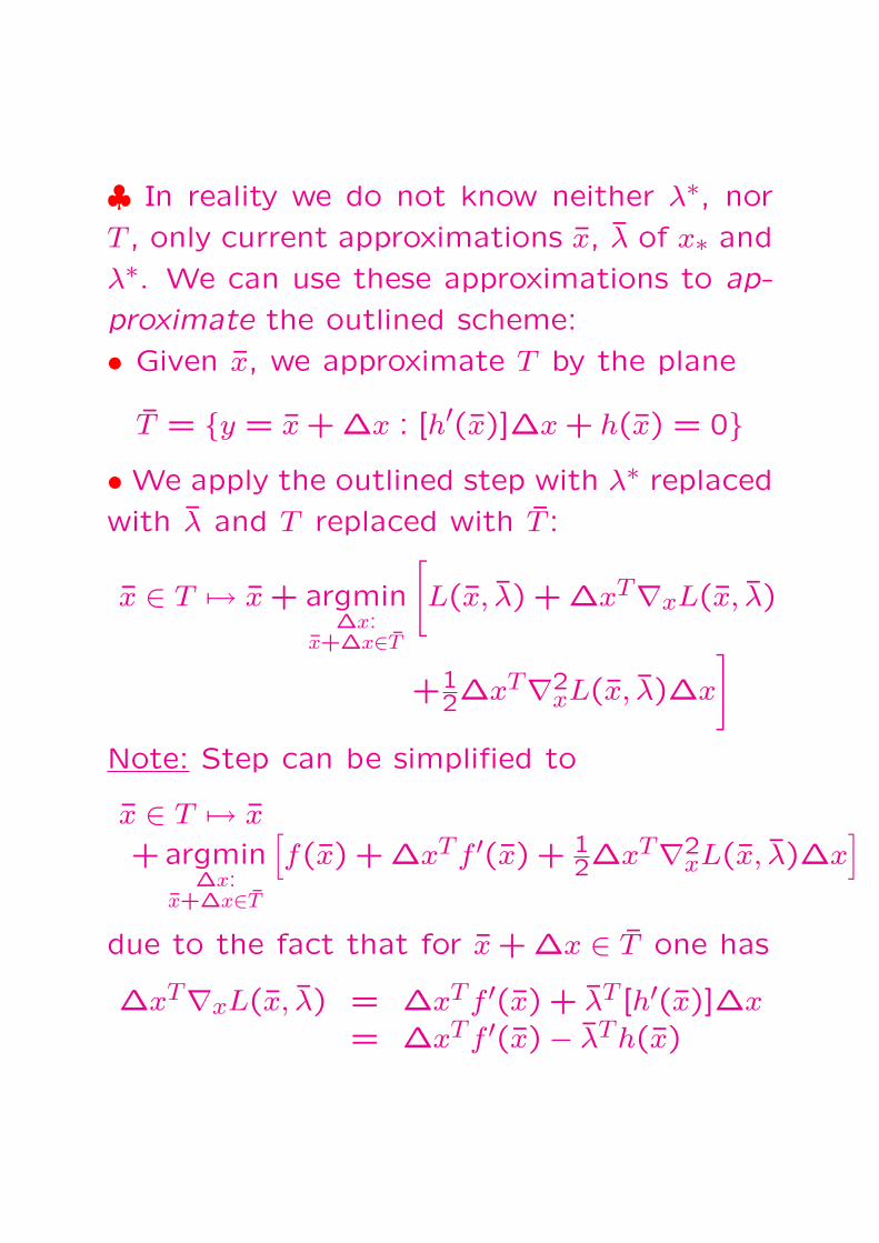
♣ In reality we do not know neither λ∗, nor
T , only current approximations x, λ of x∗ and
λ∗. We can use these approximations to ap-
proximate the outlined scheme:
• Given x, we approximate T by the plane
T = y = x + ∆x : [h′(x)]∆x + h(x) = 0• We apply the outlined step with λ∗ replaced
with λ and T replaced with T :
x ∈ T 7→ x + argmin∆x:
x+∆x∈T
[L(x, λ) + ∆xT∇xL(x, λ)
+12∆xT∇2
xL(x, λ)∆x
]
Note: Step can be simplified to
x ∈ T 7→ x
+argmin∆x:
x+∆x∈T
[f(x) + ∆xTf ′(x) + 1
2∆xT∇2xL(x, λ)∆x
]
due to the fact that for x + ∆x ∈ T one has
∆xT∇xL(x, λ) = ∆xTf ′(x) + λT [h′(x)]∆x
= ∆xTf ′(x)− λTh(x)
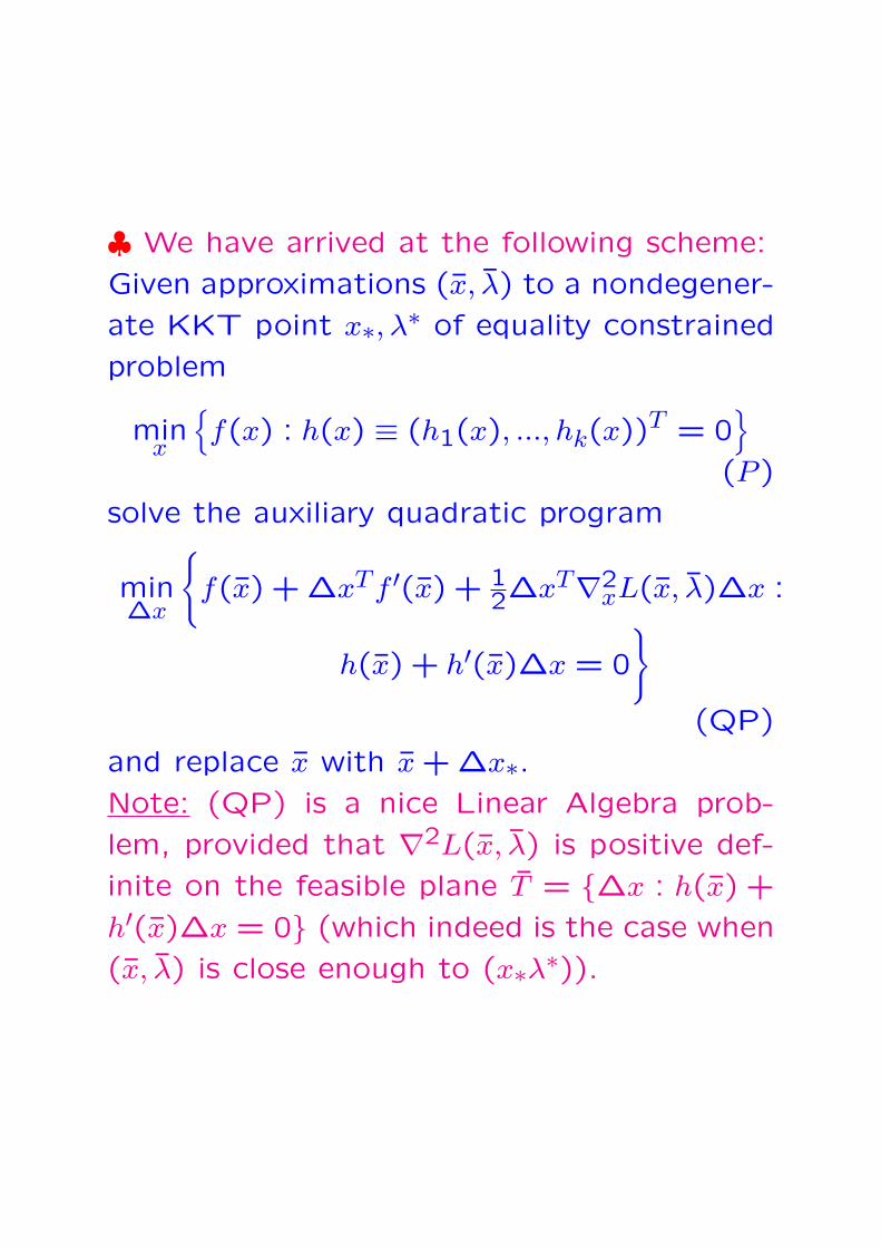
♣ We have arrived at the following scheme:
Given approximations (x, λ) to a nondegener-
ate KKT point x∗, λ∗ of equality constrained
problem
minx
f(x) : h(x) ≡ (h1(x), ..., hk(x))
T = 0
(P )
solve the auxiliary quadratic program
min∆x
f(x) + ∆xTf ′(x) + 1
2∆xT∇2xL(x, λ)∆x :
h(x) + h′(x)∆x = 0
(QP)
and replace x with x + ∆x∗.Note: (QP) is a nice Linear Algebra prob-
lem, provided that ∇2L(x, λ) is positive def-
inite on the feasible plane T = ∆x : h(x) +
h′(x)∆x = 0 (which indeed is the case when
(x, λ) is close enough to (x∗λ∗)).
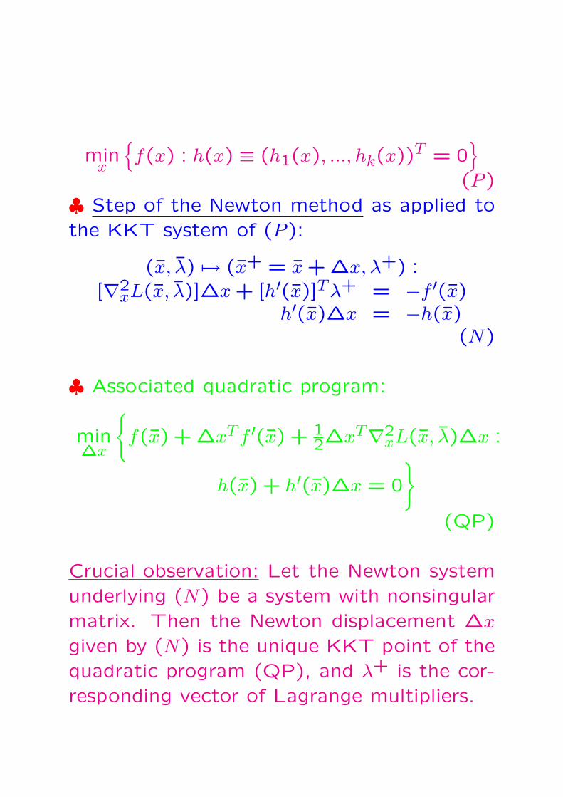
minx
f(x) : h(x) ≡ (h1(x), ..., hk(x))
T = 0
(P )♣ Step of the Newton method as applied tothe KKT system of (P ):
(x, λ) 7→ (x+ = x + ∆x, λ+) :[∇2
xL(x, λ)]∆x + [h′(x)]Tλ+ = −f ′(x)h′(x)∆x = −h(x)
(N)
♣ Associated quadratic program:
min∆x
f(x) + ∆xTf ′(x) + 1
2∆xT∇2xL(x, λ)∆x :
h(x) + h′(x)∆x = 0
(QP)
Crucial observation: Let the Newton systemunderlying (N) be a system with nonsingularmatrix. Then the Newton displacement ∆x
given by (N) is the unique KKT point of thequadratic program (QP), and λ+ is the cor-responding vector of Lagrange multipliers.
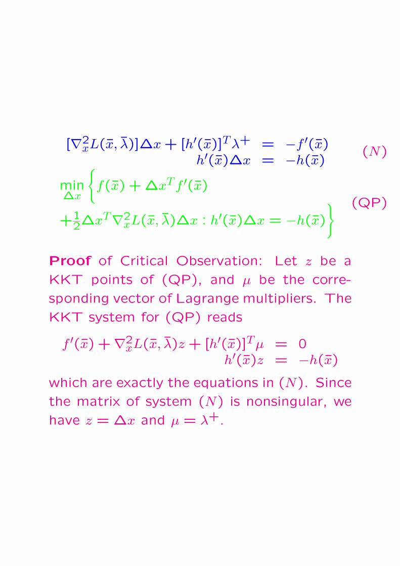
[∇2xL(x, λ)]∆x + [h′(x)]Tλ+ = −f ′(x)
h′(x)∆x = −h(x)(N)
min∆x
f(x) + ∆xTf ′(x)
+12∆xT∇2
xL(x, λ)∆x : h′(x)∆x = −h(x)
(QP)
Proof of Critical Observation: Let z be a
KKT points of (QP), and µ be the corre-
sponding vector of Lagrange multipliers. The
KKT system for (QP) reads
f ′(x) +∇2xL(x, λ)z + [h′(x)]Tµ = 0
h′(x)z = −h(x)
which are exactly the equations in (N). Since
the matrix of system (N) is nonsingular, we
have z = ∆x and µ = λ+.
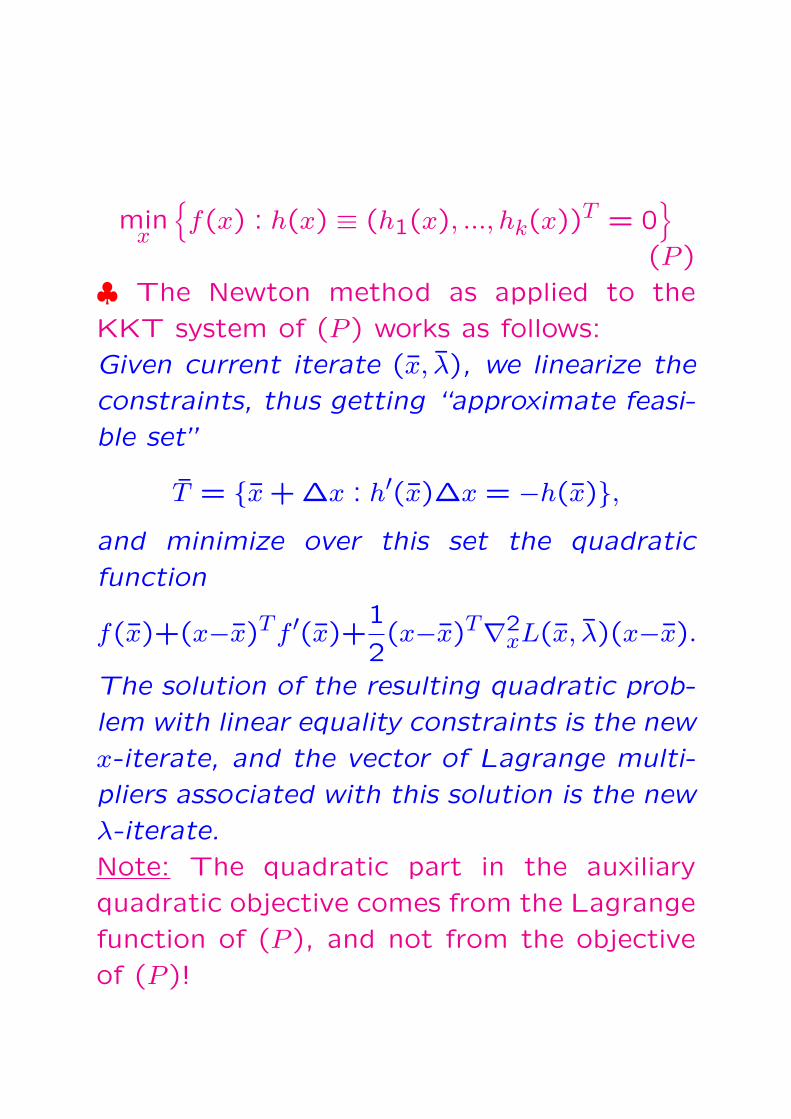
minx
f(x) : h(x) ≡ (h1(x), ..., hk(x))
T = 0
(P )
♣ The Newton method as applied to the
KKT system of (P ) works as follows:
Given current iterate (x, λ), we linearize the
constraints, thus getting “approximate feasi-
ble set”
T = x + ∆x : h′(x)∆x = −h(x),and minimize over this set the quadratic
function
f(x)+(x−x)Tf ′(x)+1
2(x−x)T∇2
xL(x, λ)(x−x).
The solution of the resulting quadratic prob-
lem with linear equality constraints is the new
x-iterate, and the vector of Lagrange multi-
pliers associated with this solution is the new
λ-iterate.
Note: The quadratic part in the auxiliary
quadratic objective comes from the Lagrange
function of (P ), and not from the objective
of (P )!
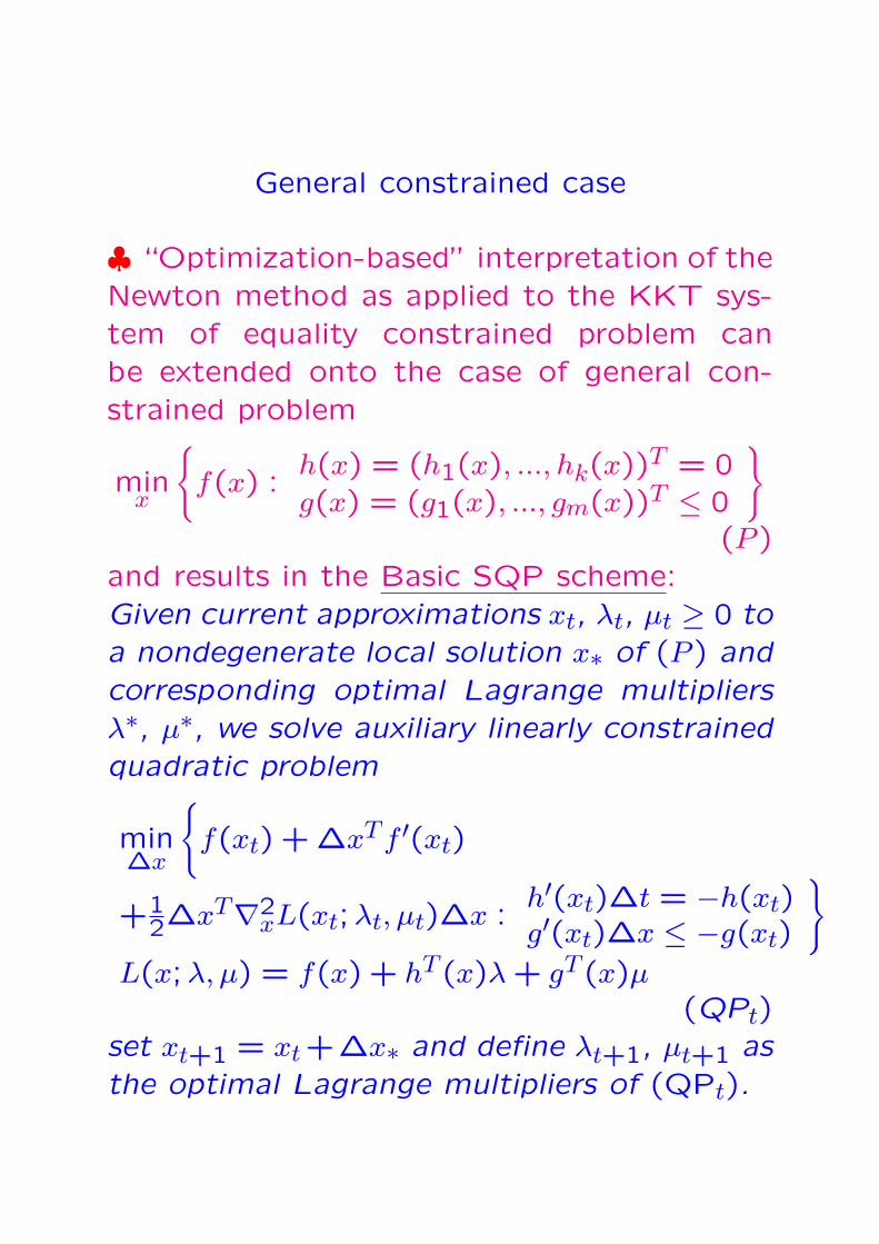
General constrained case
♣ “Optimization-based” interpretation of theNewton method as applied to the KKT sys-tem of equality constrained problem canbe extended onto the case of general con-strained problem
minx
f(x) :
h(x) = (h1(x), ..., hk(x))T = 0
g(x) = (g1(x), ..., gm(x))T ≤ 0
(P )and results in the Basic SQP scheme:Given current approximations xt, λt, µt ≥ 0 toa nondegenerate local solution x∗ of (P ) andcorresponding optimal Lagrange multipliersλ∗, µ∗, we solve auxiliary linearly constrainedquadratic problem
min∆x
f(xt) + ∆xTf ′(xt)
+12∆xT∇2
xL(xt;λt, µt)∆x :h′(xt)∆t = −h(xt)g′(xt)∆x ≤ −g(xt)
L(x;λ, µ) = f(x) + hT (x)λ + gT (x)µ(QPt)
set xt+1 = xt+∆x∗ and define λt+1, µt+1 asthe optimal Lagrange multipliers of (QPt).

minx
f(x) :
h(x) = (h1(x), ..., hk(x))T = 0
g(x) = (g1(x), ..., gm(x))T ≤ 0
(P )
Theorem. Let (x∗;λ∗, µ∗) be a nondegenerate
locally optimal solution to (P ) and the corre-
sponding optimal Lagrange multipliers. The
Basic SQP method, started close enough to
(x∗;λ∗, µ∗), and restricted to work with ap-
propriately small ∆x, is well defined and con-
verges to (x∗;λ∗, µ∗) quadratically.
♣ Difficulty: From the “global” viewpoint,
the auxiliary quadratic problem to be solved
may be bad (e.g., infeasible or below un-
bounded). In the equality constrained case,
this never happens when we are close to the
nondegenerate local solution; in the general
case, bad things may happen even close to a
nondegenerate local solution.
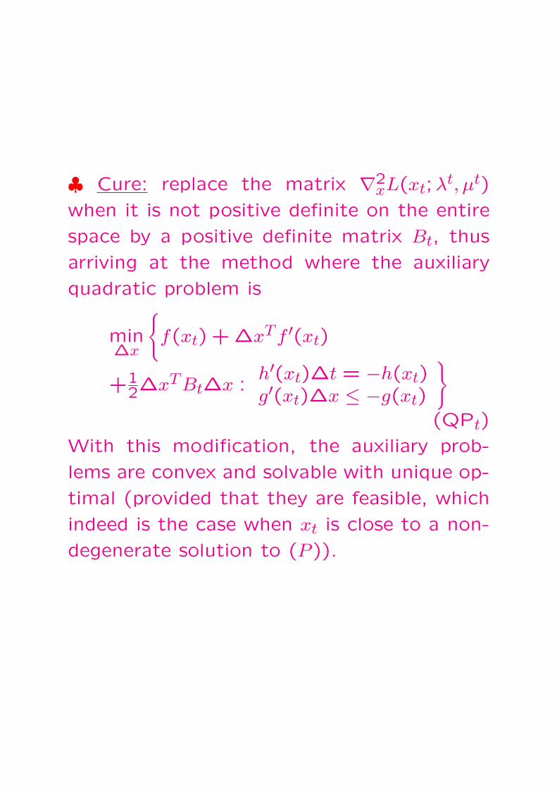
♣ Cure: replace the matrix ∇2xL(xt;λt, µt)
when it is not positive definite on the entire
space by a positive definite matrix Bt, thus
arriving at the method where the auxiliary
quadratic problem is
min∆x
f(xt) + ∆xTf ′(xt)
+12∆xTBt∆x :
h′(xt)∆t = −h(xt)g′(xt)∆x ≤ −g(xt)
(QPt)
With this modification, the auxiliary prob-
lems are convex and solvable with unique op-
timal (provided that they are feasible, which
indeed is the case when xt is close to a non-
degenerate solution to (P )).

Ensuring global convergence
♣ “Cured” Basic SQP scheme possesses nice
local convergence properties; however, it in
general is not globally converging.
Indeed, in the simplest unconstrained case
SQP becomes the basic/modified Newton
method, which is not necessarily globally
converging, unless linesearch is incorporated.

♠ To ensure global convergence of SQP, we
incorporate linesearch. In the scheme with
linesearch, the solution (∆x, λ+, µ+) to the
auxiliary quadratic problem
min∆x
f(xt) + ∆xTf ′(xt)
+12∆xTBt∆x :
h′(xt)∆t = −h(xt)g′(xt)∆x ≤ −g(xt)
(QPt)
is used as search direction rather than as a
new iterate. The new iterate is
xt+1 = xt + γt+1∆x
λt+1 = λt + γt+1(λ+ − λt)
µt+1 = µt + γt+1(µ+ − µt)
where γt+1 > 0 is the stepsize given by line-
search.
Question: What should be minimized by the
linesearch?
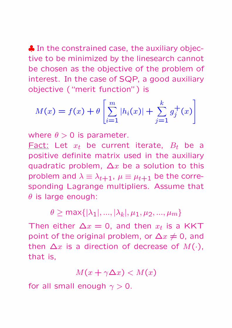
♣ In the constrained case, the auxiliary objec-tive to be minimized by the linesearch cannotbe chosen as the objective of the problem ofinterest. In the case of SQP, a good auxiliaryobjective (“merit function”) is
M(x) = f(x) + θ
m∑
i=1
|hi(x)|+k∑
j=1
g+j (x)
where θ > 0 is parameter.Fact: Let xt be current iterate, Bt be apositive definite matrix used in the auxiliaryquadratic problem, ∆x be a solution to thisproblem and λ ≡ λt+1, µ ≡ µt+1 be the corre-sponding Lagrange multipliers. Assume thatθ is large enough:
θ ≥ max|λ1|, ..., |λk|, µ1, µ2, ..., µmThen either ∆x = 0, and then xt is a KKTpoint of the original problem, or ∆x 6= 0, andthen ∆x is a direction of decrease of M(·),that is,
M(x + γ∆x) < M(x)
for all small enough γ > 0.
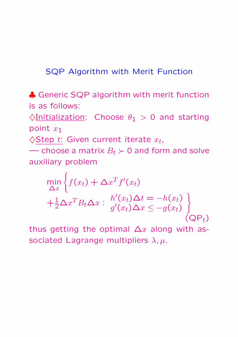
SQP Algorithm with Merit Function
♣ Generic SQP algorithm with merit function
is as follows:
♦Initialization: Choose θ1 > 0 and starting
point x1
♦Step t: Given current iterate xt,
— choose a matrix Bt  0 and form and solve
auxiliary problem
min∆x
f(xt) + ∆xTf ′(xt)
+12∆xTBt∆x :
h′(xt)∆t = −h(xt)g′(xt)∆x ≤ −g(xt)
(QPt)
thus getting the optimal ∆x along with as-
sociated Lagrange multipliers λ, µ.
— if ∆x = 0, terminate: xt is a KKT point
of the original problem, otherwise proceed as
follows:
— check whether
θt ≥ θt ≡ max|λ1|, ..., |λk|, µ1, ..., µm.if it is the case, set θt+1 = θt, otherwise set
θt+1 = max[θt,2θt];
— Find the new iterate
xt+1 = xt + γt+1∆x
by linesearch aimed to minimize the merit
function
Mt+1(x) = f(x)+θt+1
m∑
i=1
|hi(x)|+k∑
j=1
g+j (x)
on the search ray xt+γ∆x | γ ≥ 0. Replace
t with t + 1 and loop.
minx
f(x) :
h(x) = (h1(x), ..., hk(x))T = 0
g(x) = (g1(x), ..., gm(x))T ≤ 0
(P )
Theorem: Let general constrained problem
be solved by SQP algorithm with merit func-
tion. Assume that
• there exists a compact Ω ⊂ Rn such that
for x ∈ Ω the solution set D(x) of the system
of linear inequality constraints
S(x) : h′(x)∆x = −h(x), g′(x)∆x ≤ −g(x)
with unknowns ∆x is nonempty, and each
vector ∆x ∈ D(x) is a regular solution of sys-
tem S(x);
• the trajectory xt of the algorithm belongs
to Ω and is infinite (i.e., the method does not
terminate with exact KKT point);
• the matrices Bt used in the method are uni-
formly bounded and uniformly positive def-
inite: cI ¹ Bt ¹ CI for all t, with some
0 < c ≤ C < ∞.
Then all accumulation points of the trajec-
tory of the method are KKT points of (P ).
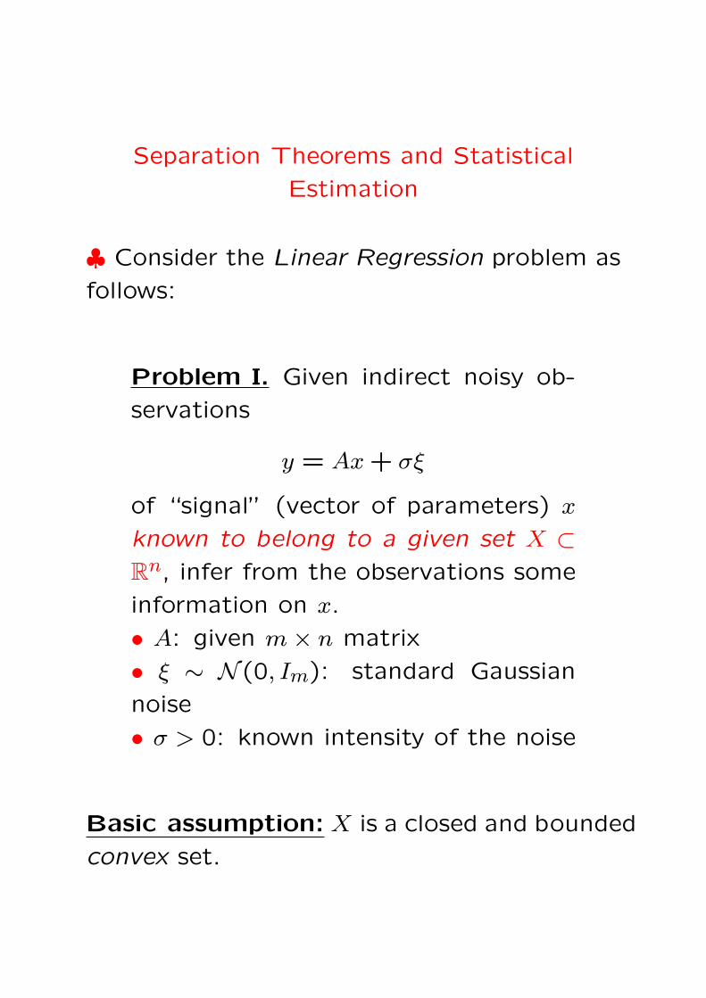
Separation Theorems and Statistical
Estimation
♣ Consider the Linear Regression problem as
follows:
Problem I. Given indirect noisy ob-
servations
y = Ax + σξ
of “signal” (vector of parameters) x
known to belong to a given set X ⊂Rn, infer from the observations some
information on x.
• A: given m× n matrix
• ξ ∼ N (0, Im): standard Gaussian
noise
• σ > 0: known intensity of the noise
Basic assumption: X is a closed and bounded
convex set.

♠ Example: Imaging
• A (discretized) 1D/2D/3D image is a func-
tion on a n-element grid of “pixels” – small
1D/2D/3D boxes. The value of this func-
tion at a pixel j is the intensity (brightness,
“blackness”, etc.) of the image in the pixel.
⇒An image is a vector x ∈ Rn, where xj is
the intensity of the “physical image’ in j-th
pixel.
• With no noise, the output of a typical scan-
ner depends linearly on the input image x,
and in many cases the noise η enters the ob-
servations z additively: z = Bx + η.
• When, as it often is the case, the noise
is Gaussian, we can pass from the obser-
vations z = Bx + η to the observations
y ≡ Cz = CBx + Cη ≡ Ax + ξ in such a way
that the Gaussian noise ξ is white: ξ ∼N (0, I).
• In many cases, a priori information, like
0 ≤ xj ≤ L, or 0 ≤ xj,∑
j xj ≤ L, allows
to localize the image in a known in advance
convex compact set X.
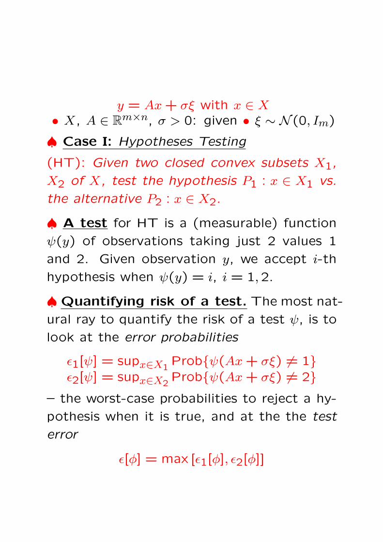
y = Ax + σξ with x ∈ X• X, A ∈ Rm×n, σ > 0: given • ξ ∼ N (0, Im)
♠ Case I: Hypotheses Testing
(HT): Given two closed convex subsets X1,
X2 of X, test the hypothesis P1 : x ∈ X1 vs.
the alternative P2 : x ∈ X2.
♠ A test for HT is a (measurable) function
ψ(y) of observations taking just 2 values 1
and 2. Given observation y, we accept i-th
hypothesis when ψ(y) = i, i = 1,2.
♠Quantifying risk of a test. The most nat-
ural ray to quantify the risk of a test ψ, is to
look at the error probabilities
ε1[ψ] = supx∈X1Probψ(Ax + σξ) 6= 1
ε2[ψ] = supx∈X2Probψ(Ax + σξ) 6= 2
– the worst-case probabilities to reject a hy-
pothesis when it is true, and at the the test
error
ε[φ] = max [ε1[φ], ε2[φ]]
y = Ax + σξ with x ∈ X• X, A ∈ Rm×n, σ > 0: given • ξ ∼ N (0, Im)
♣ Solving HT. Let Yi = AXi, i = 1,2. Yi
are closed convex compact sets along with
X1 and X2. We can separate them by the
widest possible stripe by solving the opti-
mization problem
Opt = minu,v
12‖u− v‖2 : u ∈ Y1, v ∈ Y2
= 12‖u∗ − v∗‖2
[u∗ ∈ Y1, v∗ ∈ Y2]
• when Opt = 0 (⇔ u∗ = v∗), the sets Y1 and
Y2 cannot be strictly separated
• when Opt > 0, setting f = u∗−v∗‖u−v‖2, e = u∗+v∗
2 ,
we have
fT [y − e]
≥ Opt, y ∈ Y1≤ −Opt, y ∈ Y2

Theorem (i) [lower bounds] The test error
of every test satisfies the inequality
ε[φ] ≥ Erf(Opt/σ),
where Erf(s) =
∞∫
s
1√2π
exp−t2/2dt is the er-
ror function.
(ii) [optimal test] Assuming Y1∩Y2 = ∅, con-
sider the test
ψ∗(y) =
1, fT (y − e) > 02, fT (y − e) < 0
Then
ε1[ψ∗] = ε2[ψ∗] = ε[ψ∗] = Erf(Opt/σ).
X1
X2
Y1
Y2
accept P1 accept P2
Proof of lower bound: We have Opt =12‖u∗ − v∗‖2 = 1
2‖A[x1 − x2]‖2, where xi ∈ Xi,
i = 1,2. Let us replace the “complex” hy-
potheses Pi : x ∈ Xi, i = 1,2, with simple hy-
potheses Πi : x = xi, i = 1,2. Every test ca-
pable to distinguish between Π1 and Π2 with
certain test error and error probabilities, dis-
tinguishes between Π1 and Π2 with the same
or smaller test error and error probabilities.
Now let us use the following simple result:
Lemma Let ψ be a test for distinguishing be-
tween two simple hypotheses Π1, Π2 on the
distribution of observation y ∈ Rm, Πi stating
that the density of the distribution is pi(y),
i = 1,2. Then
2ε[φ] ≥∫
min[p1(y), p2(y)]dy

Proof of Lemma. Consider a randomizedtest ψ which, given an observation y, acceptsΠ1 with probability p(y), and Π2 with proba-bility q(y) = 1− p(y). Then
ε1[φ] =∫
q(y)p1(y)dy
ε2[φ] =∫
p(y)p2(y)dy
⇒ 2ε[φ] ≥ ε1[φ] + ε2[φ]
=∫
[p(y)p2(y) + (1− p(y))p1(y)]dy
≥∫
min[p1(y), p2(y)]dy.
Lemma ⇒ lower bound: We are in the sit-
uation of pi(y) =[
1√2πσ
]mexp−‖y−Axi‖22
2σ2 ,i = 1,2, whence
2ε[φ] ≥∫ [
1√2πσ
]mexpmin
[−‖y−u∗‖22
2σ2 ,−‖y−v∗‖222σ2
]dy
[setting y − u∗+v∗2 = σz, h = u∗−v∗
2Opt , ρ = Opt/σ]
=∫ [
1√2π
]mexp−max[‖u−ρh‖22,‖u+ρh‖22]
2 du
= 2∫
uT h≥0
[1√2π
]mexp−‖u+ρh‖22
2 du
= 2
∞∫
0
1√2π
exp−[s+ρ]2
2 ds = 2Erf(ρ).
Upper bound: Let x ∈ X2. Then
Probψ∗(Ax + σξ) = 1≤
∫
u:fT [u−e]≥0
[1√2πσ
]mexp−‖u−Ax‖22
2σ2 du
[setting u−Ax = σz]∫
fT z≥1σfT [e−Ax]
[1√2π
]mexp−‖z‖
22
2 dz
≤∫
fT z≥Optσ
[1√2π
]mexp−‖z‖
22
2 dz
=∫
s≥Opt/σ
1√2π
exp−s2/2 = Erf(Opt/σ)
and similarly for x ∈ X1 it holds
Probψ∗(Ax + σξ) = 2≤
∫
u:fT [u−e]≤0
[1√2πσ
]mexp−‖u−Ax‖22
2σ2 du
=∫
fT z≤1σfT [e−Ax]
[1√2π
]mexp−‖z‖
22
2 dz
≤∫
fT z≤−Optσ
[1√2π
]mexp−‖z‖
22
2 dz = Erf(Opt/σ)

y = Ax + σξ with x ∈ X• X, A ∈ Rm×n, σ > 0: given • ξ ∼ N (0, Im)
♠ Case II: Estimating Linear Form
(ELF): Given a linear form gT z of z ∈ Rn,
estimate gTx.
♠ An estimate for ELF is a (measurable)
function g(y) of observations taking real val-
ues; g(y) is the estimate of gTx associated
with observation y.
♠ Quantifying risk of an estimate. Most
natural ray to quantify the risk of an estimate
g(·) at a given x ∈ X is via the mean squared
estimation error E[g(Ax + σξ)− gTx]2.• Estimate g(·) on the entire X is quantified
by its worst-case, over x ∈ X, risk
Risk[g] = supx∈X
E[g(Ax + σξ)− gTx]2
• It makes sense to compare this risk with
the minimax optimal risk
Risk∗ = infg(·)
Risk[g].

♠ An estimate g(·) is called affine, if it is anaffine function of observations:
g(y) = hTy + c.
For an affine estimate, its risk at a point is
E[hT (Ax + σξ) + c− gTx]2= E
[[hTAx + c− fTx]︸ ︷︷ ︸
bias
+ σhT ξ︸ ︷︷ ︸stochastic
term
]2
=[hTAx + c− fTx
]2+ σ2‖h‖22
whence
Risk[g] =[maxx∈X
|hTAx + c− fTx|]2
+ σ2‖h‖22.
(∗)Note: When X is “computationally tractable”(e.g., is a polytope), the right hand side in(∗) can be efficiently minimized in h, c. Thus,we can “reach efficiently” the optimal esti-mation risk RiskAff∗ achievable with affineestimates.In contrast, in general it is completely un-clear how to reach the minimax optimal riskRisk∗ – the underlying estimate “exists in thenature”, but we have no idea what is it.
Theorem [D. Donoho, 1994] RiskAff∗ is
within absolute constant factor (in fact, 5/4)
of Risk∗.Note: When estimating the signal itself rather
than an affine form of the signal, the risks of
affine estimates can be incomparably worse
than the risks of non-affine ones...
Proof of Donoho’s Theorem. 1. It is eas-
ily seen that we can normalize the situation
by assuming σ = 1 and that RiskAff∗ > 1;
all we need to prove that in this normalized
situation Risk∗ ≥ O(1).
2. Replacing Rn with Aff(X), we may as-
sume that intX 6= ∅. Let X∗ = X − X, so
that X∗ is a convex compact set symmetric
w.r.t. 0 ∈ intX. Thus, X∗ is the unit ball of
a norm p(·) on Rn. Let
p∗(u) = maxz
uT z : p(z) ≤ 1
≡ maxz
uTx : z ∈ X∗
≡ maxx,x′uT [x− x′] : x, x′ ∈ X
be the conjugate norm.

General fact: For every norm p(·) on Rn, itstwice conjugate norm (p∗)∗(·) is p(·) itself.Proof. From definition of the conjugatenorm it follows that
∀(u, v) : |uTv| ≤ p(u)p∗(v).Therefore
(p∗)∗(u) = maxv:p∗(v)≤1
vTu ≤ maxv:p∗(v)≤1
p(u)p∗(v)
≤ p(u).
It remains to lead to a contradiction the as-sumption that (p∗)∗(u) < p(u) for certain u.Indeed, assume that it is the case. By ho-mogeneity, we may assume that p(u) > 1,while (p∗)∗(u) < 1. Since p(u) > 1, we canstrongly separate u and the unit ball of p(·):there exists v such that
vT u > maxu:p(u)≤1
vTu = p∗(v).
But then
p∗(v) < vT u ≤ p∗(v)(p∗)∗(u),
whence
(p∗)∗(u) ≥ 1,
which is a desired contradiction.
3. Let us verify that when α ≥ 0, β ≥ 0 are
such that α2 + β2 ≤ 1, no h ∈ Rm satisfies
p∗(ATh− g) ≤ 2α and ‖h‖2 ≤ β.
Indeed, assume such an h exists. Then
2α
≥ p∗(ATh− g) = maxx,x′∈X
[ATh− g]T [x− x′]
= maxx∈X
[ATh− g]Tx−minx∈X
[ATh− g]Tx.
Setting
c = −1
2
[maxx∈X
[ATh− g]Tx + minx∈X
[ATh− g]Tx
],
we conclude that
maxx∈X
|[hTAx + c]− gTx| ≤ α,
whence for the affine estimate g(y) = hTy+c
one has
Risk[g] ≤ α2 + β2 = 1,
which is impossible, since RiskAff∗ > 1.
4. We have seen that when α2 + β2 = 1 andα, β ≥ 0, no h satisfies the relations
p∗(ATh− g) ≤ 2α and ‖h‖2 ≤ β,
meaning that the compact convex sets
u : p∗(u− g) ≤ 2α, ATh : ‖h‖2 ≤ βcan be strongly separated:
∃z : minu:p∗(u−g)≤2α
uT z > max‖h‖2≤β
(ATh)T z
We have
max‖h‖2≤β
(ATh)T z = max‖h‖2≤β
hT (Az) = β‖Az‖2and
minu:p∗(u−g)≤2α
uTz = mind:p∗(d)≤2α
[gT z + dT z]
= gT z − 2α(p∗)∗(z) = gT z − 2αp(z).
Thus, gT z − 2αp(z) > β‖Az‖2. This inequalityremains valid when z is replaced with θz, θ >
0; thus, we may assume that p(z) = 1, i.e.,z = r − s with r, s ∈ X. The bottom line is:
∀(α ≥ 0, β ≥ 0, α2 + β2 = 1) :∃r, s ∈ X : gT [r − s] ≥ 2α + β‖A[r − s]‖2.

5. Setting α = β =√
1/2, we get
∃r, s ∈ X : gT [r − s] >√
2 +1√2‖A[r − s]‖2.
(!)
We claim that then
∃u, v ∈ X : gT [u− v] ≥√
2 and ‖A[u− v]‖2 ≤ 2.
Indeed, when ‖A[r − s]‖2 ≤ 2, we can take
u = r, v = s. When ‖A[r − s]‖2 > 2, we can
set u = s + 2‖A[r−s]‖2[r − s], v = s, so that
‖A[u− v]‖2 = 2‖A[r−s]‖2‖A[r − s]‖2 = 2 and
gT [u− v] = 2‖A[r−s]‖2gT [r − s]
≥ 2‖A[r−s]‖2
1√2‖A[r − s]‖2 =
√2.
6. Since ‖A[u− v]‖2 ≤ 2, for every test ψ for
distinguishing between the hypotheses P1 :
x = u and P2 : x = v we have ε[ψ] ≥ Erf(1).
Now let g(·) be an estimate of gTx, and let
ψ(y) =
1, g(y) ≥ gT e,
2, g(y) < gT e, e =
u + v
2.
When x = u and the test accepts P2, we have
g(y) ≤ gT e, while
gTx = gT r = gT e +1
2gT [u− v] ≥ gT e +
1√2
,
that is, the squared estimation error is ≥ 1/2,
whence
ε1[ψ] ≤ Risk[g]
1/2= 2Risk[g].
Similarly, when x = v and the test accepts
P1, we have g(y) ≥ gT e and gTx = gTv =
gT e− 12gT [u− v] ≤ gT e− 1√
2, whence
ε2[ψ] ≤ Risk[g]
1/2= 2Risk[g].
Thus,
2Risk[g] ≥ ε[ψ] ≥ Erf(1) ⇒ Risk[g] ≥ Erf(1)/2.
Since g is an arbitrary estimate, we get
Risk∗ ≥ O(1).

♣ Illustration: Participles detection
Situation: A stream of participles contami-nated by “background signal” inputs a de-tector. The output of the detector with nooutput noise is
z(t) =∫ ∆
0D(t− s)
∑
j
µjδ(s− sj) + w(s)
ds
where• µj is the energy of j-th participle, sj is themoment when it arrives and δ(·) is the Diracδ-function• w(·) is the “background signal”• D(·) is the “impulse response” of the de-tector – its output when the input is δ(·). Weassume D(t) to be supported on [0,∆].♠ After discretization in time with resolutionδt = ∆/N , the model becomes
yτ =∑
` [µ` + w`δt]Dτ−` + σξτ
µ` : energy of participle arriving at time ` · δt
ξτ ∼ N (0,1)∞τ=−∞ : independent output noises
w` = w(` · δt), Dr = D(r · δt), σ > 0 : noise level
The goal: To infer from observations infor-mation on µτ∞τ=−∞.

yτ =∑
` [µ` + w`δt]Dτ−` + σξτ
♠ Strategy:
• We fix a number K of consecutive “kernel
widths” to be considered, thus focusing on
recovering µτ ’s for 0 ≤ τ ≤ KN − 1. Obser-
vations at these instants are defined, up to
observation noise, by two vectors
µ = [µ−N+1;µ−N+2; ...;µKN−1]w = [w−N+1;w−N+2; ...;wKN−1]
according to
[y0; ...; yKN−1] ≡ y = A[µ;w] + σξ
[ξ ∼ N (0, IKN)]
• Assume we know an upper bound µ on par-
ticiple’s energy and an upper bound n on the
number of participles which can arrive at in-
stants −N + 1,−N + 2, ..., KN − 1. Then µ
belongs to the convex compact set
M =
µ ∈ R(K+1)N−1 :
µ ≥ 0, µτ ≤ µ,∑τ µτ ≤ nµ

• We model the background signal w(t) as
smooth with given parameters of smooth-
ness, say, twice differentiable with |w(·)| ≤ C0
and |w′′(·)| ≤ C2, which translates into the
restriction
w ∈ W =
w :|wτ | ≤ C0, −N + 1 ≤ τ < KN
|wτ − 2wτ+1 + wτ+2| ≤ C2δt2,−N + 1 ≤ τ < KN − 2
.
• Thus, we arrive at the situation where we
are given noisy indirect observations
y = Ax + σξ [x = [µ;w]]
of a signal x ∈ X = M×W and are interested
to recover linear forms
gTτ [µ;w] = µτ
of the signal.
Note: In fact, it suffices to find a single
τ = τ∗ for which µτ can be well estimated via
our observations y−N+1, ..., yKN−1. Given the
corresponding estimate g, we can estimate µτ
for every τ by the quantity
g(yτ−τ∗−N+1, ..., yτ−τ∗+KN−1).

♠ Numerical illustration:
Setup:
• Impulse response D(s) = c [expas − expbs],0 ≤ s ≤ 1.
• Discretization: N = 40 grid points per 1
sec (δt = 1/40)
0 5 10 15 20 25 30 35 400
0.1
0.2
0.3
0.4
0.5
0.6
0.7
0.8
0.9
1
Impulse response
• K = 2, i.e., 80 observations and dimµ =
dimw = 119
• Participles: µτ ∈ [0, µ = 0.2], with at most
n = 5 participles per 119 consecutive discrete
time instants
• Background signal: |w(·)| ≤ 1, |w′′(·)| ≤ 1
• Noise intensity: σ = 4.33e-4

Results:• The best position for estimating µτ : τ =41. The estimate of µτ :
µτ = 0.0068 +79∑
i=0hiyτ−41−i
0 10 20 30 40 50 60 70 80−4
−3
−2
−1
0
1
2
3
Estimation weights hi
• Risk of the estimate:
0.01062 = 0.01042 + σ2 · 4.65752
• Sample recovery:
40 60 80 100 120 140 160 180 200 220−0.2
−0.15
−0.1
−0.05
0
0.05
0.1
0.15
0.2
0.25
0.3
• *: input • -·-: output • o: recovery
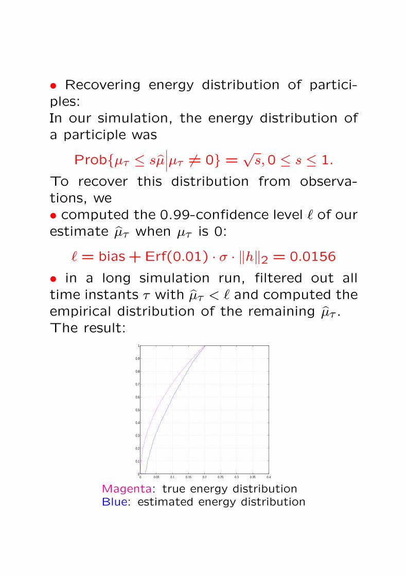
• Recovering energy distribution of partici-ples:In our simulation, the energy distribution ofa participle was
Probµτ ≤ sµ∣∣∣µτ 6= 0 =
√s,0 ≤ s ≤ 1.
To recover this distribution from observa-tions, we• computed the 0.99-confidence level ` of ourestimate µτ when µτ is 0:
` = bias + Erf(0.01) · σ · ‖h‖2 = 0.0156
• in a long simulation run, filtered out alltime instants τ with µτ < ` and computed theempirical distribution of the remaining µτ .The result:
0 0.05 0.1 0.15 0.2 0.25 0.3 0.35 0.40
0.1
0.2
0.3
0.4
0.5
0.6
0.7
0.8
0.9
1
Magenta: true energy distributionBlue: estimated energy distribution
Recommended