On the Welfare Implications of Automation
November 13, 2017
Abstract: We document that the decline in the labor income share since the 1950s has been countered by
a rise in the income share of capital goods that embody information and communication technology (ICT).
In parallel, there has been substantial reallocation of labor income from occupations relatively substitutable
with ICT (routine) to ones relatively complementary (non-routine). These trends are consistent with the
view that ICT allows for the mechanization of tasks that traditionally required labor, a process known as
automation. Our calibration suggests that automation can account for half of the decline in the labor share,
but that it is unlikely to be the sole driver of the decline in the routine labor income share. A representative
agent framework suggests welfare gains of 4%.
JEL: E25, E22, J24, J31, O33
Keywords: job polarization, elasticity of substitution between capital and labor, elasticity of substitution
between different types of labor, growth accounting
Maya Eden1
Brandeis Univeristy
Department of Economics
415 South Street
Waltham, MA 02453
Email: [email protected]
Paul Gaggl1
University of North Carolina at Charlotte
Belk College of Business
Department of Economics
9201 University City Blvd
Charlotte, NC 28223-0001
Email: [email protected]
1We would like to thank two anonymous referees as well as Greg Kaplan (the editor) for their extremely helpful comments.We are further grateful to Eric Bartelsman, Paul Beaudry, David Berger, Ben Bridgman, Aspen Gorry, Bart Hobijn, Roberto FattalJaef, Nir Jaimovich, Aart Kraay, Aitor Lacuesta, Juan Rubio-Ramirez, Aysegul Sahin, Henry Siu, Michael Sposi, Nancy Stokey,Alan Taylor as well as seminar participants at the World Bank, Vanderbilt University, Duke University, the Stockholm School ofEconomics (SITE), American University, the U.S. Bureau of Economic Analysis, the ABCDE Conference on the Role of Theory inDevelopment Economics, the 2014 NBER Summer Institute (CRIW), the 2014 SEA Meetings, the 2016 LAEF Macroeconomicsand Business CYCLE conference (UCSB), the 4th WB-BE Research Conference on “Labor markets: Growth, Productivity andInequality”, the 2016 Econometric Society NASM, and the 2016 Vienna Macro Cafe for extremely helpful comments and sugges-tions.
1

1. Introduction
The advent of information and communication technology (ICT) is widely viewed to have had trans-
formational effects on the distribution of income across factors of production. The discussion has centered
around two mechanisms: first, ICT may have lowered the demand for tasks that can easily be automated
relative to those that cannot, thus leading to a reallocation of labor income across occupations (e.g., Autor
and Dorn, 2013).1 Second, automation—the process of mechanizing certain tasks that traditionally required
labor—may have led to the reallocation of income from labor to capital, thus lowering the labor income
share (e.g., Karabarbounis and Neiman, 2014).2 While these distributional implications are broadly consid-
ered adverse, ICT has also been celebrated as an important engine of growth over the last few decades. Thus,
the policy discussion surrounding automation has often focused on striking a balance between the growth
gains from ICT and its potential distributional implications.
In this paper, we hope to further this discussion by providing some measurements of the potential distri-
butional implications of ICT and of its potential growth benefits. We begin by documenting the evolution of
income shares for different capital and labor inputs, disaggregated based on their relationship with ICT (see
Figure 1 and Table 1). We find a substantial reallocation of income from routine labor, which is relatively
more substitutable with ICT, to non-routine labor, which is relatively less substitutable with ICT, driven both
by changes in employment and by changes in average wages. In addition, we document a steep increase in
the income share of ICT capital, while the income shares of other capital types have remained trendless.
We then offer a structural interpretation of the observed trends, which allows us to comment on the
effects of automation. In particular, our quantitative analysis suggests that, in recent decades, ICT has been
responsible for about a third of output growth and about half of the decline in the labor income share. These
findings inform the policy debate on the welfare effects of automation by providing some estimates both of
the growth gains from ICT and of its implications for the distribution of income between capital and labor.
Our analysis further suggests that it is unlikely that automation is the sole driver of the decline in the
routine labor income share. We illustrate this by considering a model in which changes in the income share
1While many older contributions provide mostly conditional correlations, Akerman, Gaarder and Mogstad (2015) as well asGaggl and Wright (2017) are two recent examples providing estimates for the causal effects of ICT investments on the employmentand wage distribution. Their estimates confirm many of the earlier results (based mostly on conditional correlations) surveyed byAcemoglu and Autor (2011).
2Further examples are Elsby, Hobijn and Sahin (2013) as well as Bridgman (2014).
2

Figure 1: The Division of Income in the US(A) Labor’s Income Share (B) Capital’s Income Share
20
30
40
50
60
70
Inco
me
Sh
are
(%
of
GD
P)
1970 1980 1990 2000 2010 2020
Year
Routine Occupations
Non−Routine Occupations
Labor Share
01
02
03
04
0In
co
me
Sh
are
(%
of
GD
P)
1950 1960 1970 1980 1990 2000 2010Year
ICT Share
Non−ICT Share
Capital Share
Notes: Occupation specific income shares are based on CPS earnings data from the annual march supplement (1968 and after) andrescaled to match the aggregate income share in the Non-Farm Business Sector (BLS). Non-routine workers are those employedin “management, business, and financial operations occupations”, “professional, technical, and related occupations”, and “serviceoccupations”. Routine workers are those in “sales and related occupations”, “office and administrative support occupations”, “pro-duction occupations”, “transportation and material moving occupations”, “construction and extraction occupations”, and “installation,maintenance, and repair occupations” (Acemoglu and Autor, 2011). For details see Section 3. The construction of capital-type spe-cific income shares is described in Section 2. The underlying data are nominal gross capital stocks and depreciation rates, drawnfrom the BEA’s detailed fixed asset accounts.
Table 1: The Division of Income in the US
Labor Share Capital ShareLabor Share (%) Capital Share (%) Routine (%) Non-Routine (%) ICT (%) Non-ICT (%)
A. Raw Data1950 63.56 36.44 0.63 35.801967 63.04 36.96 37.25 25.78 1.20 35.772013 57.05 42.95 20.68 36.37 4.10 38.85
Percentage Point Change1967-2013 -5.99 5.99 -16.57 10.58 2.90 3.081950-2013 -6.52 6.52 3.47 3.05
B. Hodrick-Prescott Trend1950 64.80 35.19 0.51 35.031967 63.85 36.13 37.93 26.07 1.18 34.892013 58.04 41.95 20.82 37.15 4.04 38.24
Percentage Point Change1967-2013 -5.81 5.82 -17.11 11.08 2.86 3.361950-2013 -6.76 6.76 3.53 3.21
Notes: The table summarizes the long run trends in labor and cpaital shares as depicted in Figure 1. See the notes to Figure1 for details on the data construction. Since our earnings data based on the CPS start in 1967 we report the disaggregatedlabor shares only for the period 1967-2013. Panel A is based on raw data values while panel B uses a Hodrick-Prescott trendto remove cylicality.
3

of routine labor are driven solely by changes in relative factor supplies, in particular the increase in the ICT
capital stock. We find that this model is difficult to reconcile with the data given a standard nested CES
production framework. While, under some measurement assumptions, it is possible to match the observed
trends, doing so requires a very high elasticity of substitution between routine and non-routine labor, which
is arguably unrealistic. This suggests that other sources may be contributing to the trend in routine labor
income. For example, Autor, Dorn and Hanson (2013) emphasize the potential roles of offshoring and
international trade.
This paper is most closely related to the literature on the general equilibrium effects of declining capital
prices (e.g., Krusell, Ohanian, Rıos-Rull and Violante, 2000; Autor and Dorn, 2013; Karabarbounis and
Neiman, 2014). Our main departure from this literature is an explicit focus on the distinction between ICT
and non-ICT (NICT) capital. Karabarbounis and Neiman (2014) and Autor and Dorn (2013) consider an
aggregate capital input. Closer to our decomposition, Krusell et al. (2000) and vom Lehn (2015) distinguish
between equipment and structures. The ICT capital class considered in this paper is a subset of the broader
class of equipment. Our focus on this narrower category is motivated by the rich literature emphasizing that
ICT features unique interactions with different types of labor (Acemoglu and Autor, 2011; Akerman et al.,
2015; Gaggl and Wright, 2017). While the analysis in Krusell et al. (2000) does not find an effect on the
labor income share, our model suggests that ICT changes the distribution of income between capital and
labor, consistent with Karabarbounis and Neiman (2014).
2. Decomposing The Capital Income Share
Our approach for disaggregating the capital income share follows Hall and Jorgenson (1967) and Chris-
tensen and Jorgenson (1969).3 Suppose that there are several types of capital, denoted Ki, with i = 1, ..., I .
If aggregate income is divided between capital and labor, then the share of payments to capital must satisfy
the following relation:
sK,t =
I∑i
Ri,tKi,t
PtYt= 1− sL,t, (1)
3For a few more recent contributions that use the same basic strategy to compute the return to specific types of captial in variouscontexts see for example Jorgenson (1995), O’Mahony and Van Ark (2003), and Caselli and Feyrer (2007). We outline the basicidea of our implementation to measure capital type specific income shares here and provide detailed derivations in Appendix B.
4

where sK,t and sL,t denote the aggregate capital and labor income shares, respectively, PtYt denotes nominal
output, and Ri,t denotes the nominal rental rate of capital type i.
A no-arbitrage condition between different assets implies that, for every capital type i,
Ri,t + Pi,t+1(1− δi,t)Pi,t
= 1 + rt, (2)
where rt is the market interest rate, δi,t is the depreciation rate and Pi,t is its nominal price of a unit of
capital. The left hand side is the rate of return on a unit of capital of type i, which is purchased at the price
Pi,t, rented out for a period and resold. The right hand side is the market return on investment. We show in
Appendix B how equations (1) and (2) allow us to compute an income share for each type of capital, defined
as si,t = Ri,tKi,t/(PtYt), using the labor income share, nominal current cost values for each type of capital,
capital-specific depreciation rates, and capital-specific price indexes.
To measure the current cost values of different types of assets, we use the BEA’s detailed fixed asset
accounts.4 We aggregate the BEA’s detailed industry-level estimates into three types of capital, classified ac-
cording to the BEA’s definition: residential assets, consumer durables and non-residential assets. Within the
non-residential and consumer durables categories, we distinguish between ICT and non-ICT (NICT) assets.
Within non-residential assets, we consider an asset to be ICT if the BEA classifies it as software (classifica-
tion codes starting with RD2 and RD4) or as equipment related to computers (classifications codes starting
with EP and EN). See Tables A.7 and A.8 in Appendix A for complete lists of the detailed assets grouped
into the two types of non-residential capital. Within consumer durables, we classify the following assets
as ICT: PCs and peripherals (1RGPC); software and accessories (1RGCS); calculators, typewriters, other
information equipment (1RGCA); telephone and fax machines (1OD50).5 Our definition of ICT capital is
4Official documenation for the BEA’s methodology to construct these estimates is available athttp://www.bea.gov/national/pdf/Fixed Assets 1925 97.pdf. Most macroeconomic studies using capital stocks utilize a sim-pler version of the perpetual inventory method than the BEA’s estimates, usually based on linear constant depreciation andaggregate real investment rates. We prefer the BEA’s estimates for several reasons: first, they are provided at the detailed assetlevel; second, they allow for time varying non-linear depreciation patterns; finally, these estimates allow us to directly use nominalstocks at current cost, rather than chain-weighted quantity indexes.
5We note that it is difficult to identify robots in the BEA classification. Industrial robots are perhaps the most relevant typeof robot within our context, especially in the earlier part of our sample. The International Robot Association defines this type ofcapital as “automatically controlled reprogrammable, multifunctional manipulator with at least three programmable axes whichmay be either fixed in place or mobile for use in industrial automation applications” (as defined in the standard ISO 8373: 1994).Given the BEA’s asset classification these robots are most likely classified as “industrial machinery”, which we calssify as NICT.However, the software components of the robots are classified in the software category, which we identify as ICT. Thus, within our
5

Figure 2: Relative Prices & Depreciation(A) Relative Capital Prices (B) Depreciation Rates
0.5
11.5
2P
rice Index R
ela
tive to G
DP
Deflato
r
1950 1960 1970 1980 1990 2000 2010Year
ICT Capital
Non−ICT Capital
510
15
20
Depre
cia
tion R
ate
(%
)
1950 1960 1970 1980 1990 2000 2010Year
ICT Capital
Non−ICT Capital
Notes: Panel A graphs implicit price deflators by capital type expressed as a fraction of the GDP deflator, which were constructeddirectly from the BEA’s detailed fixed-asst accounts. The BEA GDP deflator is taken from FRED. Panel B depicts asset-specificdepreciation rates constructed directly from the BEA’s fixed asset accounts. See Tables A.7 and A.8 in Appendix A and the text forour grouping of assets.
in line with other available estimates of ICT, which we briefly discuss in Appendix E.
We measure the price indexes, Pi,t, and the depreciation rates, δi,t, directly from the BEA’s fixed asset
accounts.6 Panel A of Figure 2 depicts the path of prices for ICT and NICT assets relative to the GDP
deflator. This figure reveals that while the price of NICT capital relative to output remained essentially
constant throughout the entire sample, the relative price of ICT capital has fallen substantially. Panel B
of Figure 2 graphs the respective depreciation rates for each type of capital. The depreciation rate of ICT
capital is substantially higher than the depreciation rate of NICT capital and increases over time.
Panel B of Figure 1 illustrates the resulting estimates of the different capital income shares (also see
Table 1). The income share of NICT capital does not show any significant trend over the period 1950-2013.
In contrast, the income share of ICT capital has increased roughly seven-fold, from 0.63% in 1950 to 4.1%
framework, robots will show up both as ICT capital goods and as NICT capital goods that are complementary to ICT capital, whichwe comment on in Section 5.1.
6We employ implicit price deflators that we construct for each type of capital based on chain type price indices providedby the BEA to obtain a series for Pi,t. Notice that this involves constructing appropriate chain type quantity aggregates andassociated implicit price deflators for each capital type, derived from the BEA’s estimates of stocks and prices for the detailedassets listed in Tables A.7 and A.8 in Appendix A. We use Fisher’s “ideal” formula to compute these chained aggregates. Wemeasure depreciation rates based on the BEA’s nominal values for depreciation and net capital stocks. That is, we compute δi,t =(Pi,tDepi,t)/(Pi,tNetStock i,t+Pi,tDepi,t). Since both measures are reported in year-end nominal values, the price terms cancel.
6

Figure 3: Capital and its Rental Rate(A) Capital Stock Relative to 1968 (B) Rental Rate of Capital
010
20
30
40
50
Chain
Index (
1968=
1)
1950 1960 1970 1980 1990 2000 2010Year
ICT Capital
Non−ICT Capital
010
20
30
40
50
Real R
enta
l R
ate
(%
)
1950 1960 1970 1980 1990 2000 2010Year
ICT Capital
Non−ICT Capital
Notes: Panel A graphs the stock of ICT and NICT captial relative to its 1968 level. Panel B depicts asset-specific real rental rates(Ri,t/Pt) in % of final output, derived from expressions (B.5)-(B.6) in Appendix B. The underyling data are the BEA’s detailedfixed-asset accounts. The dashed vertical lines indicate the year 1968.
by 2013.7
This accounting exercise suggests that roughly half of the decline in the labor income share is attributable
to the rise in the ICT income share. The remainder is due to a rapid rise in the NICT income share, partic-
ularly after 2001. Consistent with the findings of Rognlie (2015), a further decomposition of the increase
in the NICT capital income share in the post-2001 period reveals that this rise is accounted for entirely by
a rise in the income share of structures and residential capital (see Appendix C). After removing structures
and residential capital income, the NICT capital income share is stationary. If one assumes that trends in
real estate income are unrelated to automation, this measurement exercise suggests that about half of the
decline in the labor income share is potentially attributable to ICT.
We further document that the trends in the ICT and NICT income shares are primarily within-industry
phenomena. In particular, results presented in Appendix D show that the aggregate trends in ICT and NICT
income illustrated in Figure 1 and Table 1 are robust to the inclusion of industry fixed-effects. This suggests
that the disaggregated trends in the capital income shares are not merely a result of changes in industrial
composition.
7Our estimated trends are consistent with those reported in the Conference Board’s Total Economy Database (TED), coveringthe period 1990-2016, as well as the Groningen Growth and Development Centre’s (GGDC) industry growth accounts, covering1979-2003 (see Figure E.14 in Appendix E).
7

Finally, it is it instructive to decompose the payments to capital, (Ri,t/Pt)Ki,t, into a price component
and a quantity component. To this end, we construct chained quantity indexes for the stocks of ICT and
NICT capital based on Fisher’s “ideal” formula and the BEA’s fixed asset accounts. Figure 3 shows that
while the stock of ICT has increased, its rental rate has declined.
3. Decomposing The Labor Income Share
An extensive literature in labor economics distinguishes between two types of labor based on their
interactions with ICT (Acemoglu and Autor, 2011). The first type of labor executes primarily “routine”
tasks, that require following exact, pre-specified decision trees (or routines). By their very nature, these tasks
are prone to automation. The second type of labor is intensive in non-routine tasks that require judgement,
creativity or interpersonal skills, deeming them less readily prone to automation.
We measure the income shares of several occupation groups, using two alternative measures of earnings
at the occupation level from the U.S. Current Population Survey (CPS): annual earnings from the March
supplements (MARCH) starting in 1967 (provided by IPUMS, Ruggles, Alexander, Genadek, Goeken,
Schroeder and Sobek, 2010); and weekly earnings from the CPS outgoing rotation groups (ORG) starting
in 1979 (drawn from the basic monthly CPS files provided by the NBER). Panel A of Figure 4 illustrates
that the two alternative measurements result in very similar estimates of the aggregate labor share, which are
both highly correlated with the BLS’s labor share within the total non-farm business sector (which includes
benefits, pensions, etc.).
For each occupation, we divide the aggregate annual wage bill by nominal GDP to obtain the occu-
pation’s share of wage and salary earnings in aggregate income.8 We categorize occupations as “routine”
or “non-routine” based on the classification in Acemoglu and Autor (2011). That is, we consider work-
ers employed in “management, business, and financial operations occupations”, “professional, technical,
8We use CPS sampling weights to estimate the aggregate wage bill at the detailed occupation level. For the ORGs, which aredrawn from the raw CPS basic files, this requires several non-trivial adjustments to the raw data. First, since the U.S. Departmentof Labor’s (DOL) classification of occupations changes several times during our sample period, we aggregate individuals into apanel of 330 consistent occupations, designed by Dorn (2009). We thank Nir Jaimovich for providing a crosswalk between Dorn’s(2009) occupation codes and the latest Census classification that is used in the CPS since 2011. This crosswalk is the same as inCortes, Jaimovich, Nekarda and Siu (2014). Second, we follow Champagne, Kurmann and Stewart (2017) and adjust top codedearnings based on Piketty and Saez’s (2003) updated estimates of the cross-sectional income distribution. While top-coded earningsvalues may pose less of a problem in many microeconomic analyses, they potentially introduce substantial bias when estimatingthe aggregate wage bill for high-wage occupations.
8

Figure 4: Labor’s Share in Income: CPS-ORG and CPS-MARCH(A) Aggregate Labor Income Share (B) Routine/Non-Routine Income Shares
40
45
50
55
60
65
Incom
e S
hare
(%
of G
DP
)
1970 1980 1990 2000 2010Year
BLS Non−Farm Business
NIPA: Compensation of Employees (BEA:A033RC0)
CPS−ORG (R+NR)
CPS−MARCH (R+NR)
20
25
30
35
40
Incom
e S
hare
(%
of G
DP
)
1970 1980 1990 2000 2010 2020
Year
Routine (CPS−ORG)
Non−Routine (CPS−ORG)
Routine (CPS−MARCH)
Non−Routine (CPS−MARCH)
Notes: Panel A contrasts aggregate income shares (as a fraction of GDP) based on the CPS outgoing rotation groups (ORG) as wellas annual earnings from the CPS March supplement (MARCH), aggregates reported in the NIPA tables, as well as the BLS’s estimatefor the total non-farm business sector that includes benefits, self employed, proprietors income, and other non-salary labor income.The aggregate series are drawn from FRED. The series labeled “CPS-ORG (R+NR)” and “CPS-MARCH (R+NR)” are constructedfrom our occupation specific earnings based on CPS ORG and MARCH earnings. Panel B contrasts our estimates for the routineand non-routine income shares based on ORG and MARCH data, respectively.
and related occupations”, and “service occupations” as non-routine; and we define routine workers as ones
employed in “sales and related occupations”, “office, clerical, and administrative support occupations”,
“production occupations”, “transportation and material moving occupations”, “construction and extraction
occupations”, and “installation, maintenance, and repair occupations”. This classification emerges out of
an extensive literature, surveyed by Acemoglu and Autor (2011), that originated from the seminal work by
Autor, Levy and Murnane (2003). They and many other contributions in this line of research use detailed
information on the task content of at least 300 detailed occupations (depending on the study) obtained from
the Dictionary of Occupational Titles (DOT) and its successor O*Net. The classification used here is the
“consensus aggregation” suggested by Acemoglu and Autor (2011), that captures the key insights from the
more detailed micro analyses. We drop farm workers from all our analyses for comparability with the BLS
measure of the labor income share.
Finally, we proportionately rescale group-specific income shares (which originally add up to the series
labeled “CPS-ORG(R+NR)” and “CPS-MARCH(R+NR)” in panel A of Figure 4) so that they match the
share of non-farm business labor income in GDP, as estimated by the BLS. Panel B of Figure 4 presents the
resulting estimates of the routine and non-routine labor income shares. Consistent with the labor economics
9
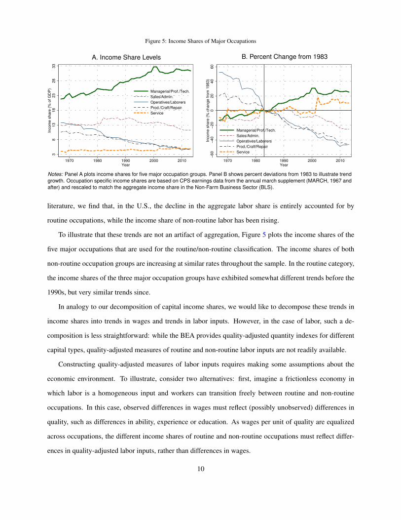
Figure 5: Income Shares of Major Occupations
A. Income Share Levels B. Percent Change from 19833
81
31
82
32
83
3In
co
me
sh
are
(%
of
GD
P)
1970 1980 1990 2000 2010Year
Managerial/Prof./Tech.
Sales/Admin.
Operatives/Laborers
Prod./Craft/Repair
Service
−6
0−
40
−2
00
20
40
60
Inco
me
sh
are
(%
ch
an
ge
fro
m 1
98
3)
1970 1980 1990 2000 2010Year
Managerial/Prof./Tech.
Sales/Admin.
Operatives/Laborers
Prod./Craft/Repair
Service
Notes: Panel A plots income shares for five major occupation groups. Panel B shows percent deviations from 1983 to illustrate trendgrowth. Occupation specific income shares are based on CPS earnings data from the annual march supplement (MARCH, 1967 andafter) and rescaled to match the aggregate income share in the Non-Farm Business Sector (BLS).
literature, we find that, in the U.S., the decline in the aggregate labor share is entirely accounted for by
routine occupations, while the income share of non-routine labor has been rising.
To illustrate that these trends are not an artifact of aggregation, Figure 5 plots the income shares of the
five major occupations that are used for the routine/non-routine classification. The income shares of both
non-routine occupation groups are increasing at similar rates throughout the sample. In the routine category,
the income shares of the three major occupation groups have exhibited somewhat different trends before the
1990s, but very similar trends since.
In analogy to our decomposition of capital income shares, we would like to decompose these trends in
income shares into trends in wages and trends in labor inputs. However, in the case of labor, such a de-
composition is less straightforward: while the BEA provides quality-adjusted quantity indexes for different
capital types, quality-adjusted measures of routine and non-routine labor inputs are not readily available.
Constructing quality-adjusted measures of labor inputs requires making some assumptions about the
economic environment. To illustrate, consider two alternatives: first, imagine a frictionless economy in
which labor is a homogeneous input and workers can transition freely between routine and non-routine
occupations. In this case, observed differences in wages must reflect (possibly unobserved) differences in
quality, such as differences in ability, experience or education. As wages per unit of quality are equalized
across occupations, the different income shares of routine and non-routine occupations must reflect differ-
ences in quality-adjusted labor inputs, rather than differences in wages.
10

Figure 6: Routine & Non-routine Labor (Relative Quantities & Prices)(A) Relative Quantities (B) NR Wage Premium
50
100
150
200
NR
/R E
mplo
ym
ent (%
of R
Em
plo
ym
ent)
1970 1980 1990 2000 2010Year
Differentiated Labor (Employment Counts)
Homogeneous Labor (NRP=0)
010
20
30
40
50
60
Non−
Routine W
age P
rem
ium
(%
)
1970 1980 1990 2000 2010Year
Differentiated Labor (Average Wage)
Homogeneous Labor (NRP=0)
Notes: Panel A plots relative employmnet (expressed as percent of routine workers) based on two alternative measurement assump-tions: the raw data and “effective” employment under the assumption of a homogeneous labor input. Panel B plots the non-routinewage premium (NRP), defined as 100 × (wnr/wr − 1), where wnr and wr represent non-routine and routine wages, for the twoalternative measurement approaches: raw CPS average wages; zero NRP by assumption.
Second, consider the opposite extreme, in which routine and non-routine labor are completely differen-
tiated inputs, and it is impossible to convert routine labor into non-routine labor (or vice versa). Given that
routine workers cannot become non-routine workers, there are no limits on the size of the premium paid to
non-routine work. In this economy, the increase in the income share of non-routine work relative to routine
work may reflect an increase in the relative quantity of non-routine labor, an increase in the relative payment
to non-routine labor, or both.
Figure 6 presents a comparison of these two alternatives. Under the assumption of homogenous labor
inputs, the wage per unit of quality-adjusted labor is equalized across occupations, and hence the rising
relative income share of non-routine labor is attributed entirely to a rise in the quality-adjusted quantity of
non-routine labor. In contrast, under the assumption of differentiated labor inputs, the rise in the relative
income share of non-routine labor is attributed both to a rise in relative labor inputs and to a rise in relative
pay. For this scenario, the measurement in Figure 6 is based on simple employment counts and average
wages, which do not take into account any changes in the composition of labor inputs. Appendix F presents
alternative ways to account for changes in observed labor composition; however, it turns out that these
alternative measurements do not affect our main results, and we therefore relegate their detailed discussion
to Appendix F.
11

4. A Calibrated Production Function
The relative stability of the NICT capital income share suggests a production function that is a Cobb-
Douglas aggregate of NICT capital (Kn) and a composite input, X , which is produced by ICT (Kc), routine
labor (Lr) and non-routine labor (Lnr). Specifically, using lower case letters to denote variables normalized
by aggregate labor (e.g., `r = Lr/L and `nr = Lnr/L, with L ≡ Lr + Lnr), we write the aggregate
production function as
y = kαnx1−α (3)
In the spirit of Krusell et al. (2000), we specify the composite x as the following nested CES aggregator:
x =[η`θr + (1− η)zθ
] 1θ (4)
z = [γkσc + (1− γ)`σnr]1σ (5)
where η, γ ∈ [0, 1] and θ, σ ≤ 1.9
To calibrate the parameters of this production function, we use the first order conditions of a compet-
itive firm. Taking wages and rental rates as given, the firm’s optimality conditions imply the following
relationships between relative quantities and relative income shares:
ln
(scsnr
)= ln
(γ
1− γ
)+ σ ln
(kc`nr
)(6)
ln
(srsz
)= ln
(η
1− η
)+ θ ln
(`rz
)(7)
where sc, snr, sr and sz are the income shares of kc, `nr, `r, and z, respectively. Our baseline approach uses
measured trends in income shares and quantities from the previous sections to calibrate the four parameters
γ, σ, η, and θ using the following two steps:10
9We note that, in principle, there are three ways to nest the CES composite x. We illustrate in Appendix G that, for thealternatives, our calibration strategy delivers parameter values that are either inconsistent with the CES asumptions or require theunrealistic assumption that routine and non-routine labor are perfect substitutes.
10As an alternative to this two step approach we also fit equations (6) and (7) jointly using GMM. The results are almost identicaland are shown in Appendix H. The GMM specification also allows us to consider trends in birth rates 15 years ago, as a possibleinstrument for trends in labor supply, following Jaimovich, Pruitt and Siu (2013). The results are virtually identical, which is notsurprising given that our strategy targets long-run trends.
12

1. Estimate γ and σ using OLS and compute the implied quantities for z
2. Estimate η and θ using OLS, based on the implied series for z from step 1
Note that this calibration strategy targets the trends in the relative income shares of ICT capital and both
routine and non-routine labor. By focusing on relative rather than absolute income shares and excluding
NICT capital, our calibration attributes only the rise in the ICT capital income share to automation, allowing
for part of the decline in the aggregate labor income share to reflect other factors.
This calibration strategy requires taking a stance on the quantities of routine and non-routine labor.
Table 2 shows the calibration results for the two alternative approaches for measuring `r and `nr detailed in
Section 3.11 Given our focus on long run trends, we eliminate short run fluctuations by using a fitted log
linear trend rather than the raw data series for all regressions shown in Table 2.12
Panel A of Table 2 reports the results under the assumption of homogeneous labor inputs, while panel
B reports the results under the assumption of differentiated labor inputs. While the first approach (panel A)
suggests an estimate of θ = 0.876 < 1, the second approach (panel B) results in a point estimate of θ > 1,
which is inconsistent with our CES production framework.
To develop intuition for these results, it is useful to observe that ICT capital income is small relative to the
income of non-routine labor. If we ignore ICT capital income, the production function of x is approximately
a two-factor CES aggregate of routine and non-routine labor (x ≈ (η`θr + (1 − η)`θnr)1/θ). If we treat
routine and non-routine labor as differentiated inputs, we are faced with a situation in which both the relative
quantity of non-routine labor and the relative wage of non-routine labor are increasing over time. This
is inconsistent with a fixed two-factor CES demand system, which requires an increase in relative factor
supplies to be met with a decrease in their relative marginal products. When, instead, we treat routine and
non-routine labor as homogeneous labor inputs, the relative wages of routine and non-routine labor are
equalized by assumption; this is consistent with the two-factor approximation x ≈ `r + `nr (or θ ≈ 1), in
which the marginal products of routine and non-routine labor are always 1. By incorporating the contribution
of ICT capital, we are able to obtain an estimate of θ < 1.
11In Appendix H we illustrate that additional alternatives, including chained quantity indexes for labor, yield results that mirrorthose based on raw employment counts and average wages. We therefore omit these results in the main text.
12We note that the results are virtually identical when we do not de-trend the data series or if we use the first and last observationonly. For transparency and in the interest of space we only report the results based on log linear trends here.
13

Table 2: Calibration of production parameters
A. Homogeneous Labor B. Differentiated Labor
(A.1) (A.2) (B.1) (B.2)
ln(scsnr
)ln
(srsz
)ln
(scsnr
)ln
(srsz
)ln (kc/`nr) 0.299*** 0.275***
(0.006) (0.005)ln (`r/z) 0.876*** 1.071***
(0.003) (0.004)Constant -5.201*** 0.138*** -5.037*** -0.100***
(0.053) (0.001) (0.046) (0.001)
Obs. 47 47 47 47
Estimated Parameters & Implied Elasticitiesγ 0.005 0.006σ 0.299 0.275EOS(kc, `nr) 1.427 1.379
η 0.535 0.475θ 0.876 1.071EOS(z, `r) 8.039
Notes: The table shows OLS estimates for the the parameters in equations(6) and (7) based on the two-step procedure described in the text: in stepone, we estimate (6); in step two, we estimate (7) conditional on the resultsfrom step one. All regressions use fitted log-linear trends as data inputs, inorder to eliminate the influence of cyclical fluctuations. Panel A assumes laborinputs are homogeneous and relative labor inputs therefore equal relative laborincome shares; panel B directly uses employment counts and average wagesfrom the CPS MARCH data. Standard errors are reported in parentheses beloweach coefficient. Significance levels are indicated by * p < 0.1, ** p < 0.05,and *** p < 0.01.
5. Counterfactual Analysis
To comment on the potential benefits of automation, we consider a representative agent model, in which
an infinitely lived household solves the following optimization problem:
maxct,kn,t+1,kc,t+1,`r,t,`nr,t,xt,zt,yt
∞∑t=0
βtu(ct)
subject to `r,t + `nr,t = 1, yt = kαnx1−αt , equations (4)-(5), and the budget constraint
ct + (1 + g)∑i
pi,tki,t+1 = yt +∑i=n,c
pi,t(1− δi,t)ki,t (8)
14

where ct is consumption per-worker and g is the growth rate of aggregate labor, Lt.
Note that, in this model, labor is a homogeneous input that is allocated optimally across routine and
non-routine occupations. We specify the model in this way for two reasons: first, because alternative spec-
ifications with differentiated labor inputs result in calibrations of the aggregate production function that are
inconsistent with the assumption of a time-invariant CES production framework (see Table 2). Second,
assuming a homogenous labor input that can be costlessly reallocated between routine and non-routine oc-
cupations is a useful benchmark for providing an upper bound on the welfare effects of automation. Since
we are simulating a representative agent framework which ignores potential distributional implications, it is
natural to focus on obtaining an upper bound.
We consider two sources of exogenous variation. The first and most relevant is the decline in the relative
price of ICT capital, pc,t. While prices are conceptually endogenous variables, in this context the price of
ICT capital can be interpreted as the real transformation rate of output into ICT capital (see also Karabar-
bounis and Neiman, 2014). The second source of exogenous variation is time variation in the depreciation
rate of ICT capital, which, as we document, is quite substantial (see Figure 2). Taken together, these two
sources of variation capture changes in the “effective” price of ICT capital from the viewpoint of an investor.
Staring from an initial steady state, we simulate the transition to a final steady state, given the paths
of the ICT capital price and its depreciation rate between 1950-2013. Along this transition, we assume a
perfect foresight equilibrium.13
We compare this baseline simulation with two sets of counterfactuals: first, we hold both the price of ICT
capital and its depreciation rate fixed at the initial steady state level. Second, we compute a counterfactual
transition in which we keep the price of ICT capital fixed but let its depreciation rate vary. This second
counterfactual allows us to disentangle the effects of the fall in the ICT capital price from the effects of the
rise in the ICT capital depreciation rate.
Our simulations are based on the calibration of the core production parameters from Section 4 (panel
A of Table 2) and the values reported in Table 3. The value of β, the discount factor, is calibrated based
13While identifying 1950 and 2013 with initial and final steady states is perhaps an oversimplification, it is worth noting that therelative price of ICT is essentially flat in the early 1950s, falls rapidly starting in the early 1960s and starts to flatten out in the mid2000s. Similarly, the rate of ICT depreciation is essentially flat at the beginning and end of our sample, but rises rapidly over theperiod 1980-2000 (see Figure 2).
15

Table 3: Calibration of Remaining Parameters
Parameter Calibration
β 0.9737u(c) ln(c)
δn 0.0733 (mean of NICT depreciation, BEA data)α 0.3505 (mean of NICT share, BEA data)g 0.0192 (trend growth in aggregate labor index; see Figure F.18)
pc,t ∈ [0.254, 1.727] (BEA data, 1950-2013)δc,t ∈ [.137, 0.206] (BEA data, 1950-2013)
Notes: The ICT price and depreciation rates are measured directly based on the BEA’s fixedasset accounts.
on our estimates of the returns to capital.14 Given our focus on long run trends, we assume log utility,
or a unitary inter-temporal elasticity of substitution, which is consistent with the wide range of empirical
estimates (see, for example, the discussion and references listed by Guvenen, 2006). For the depreciation
rate of NICT capital we take the average value of our BEA-based estimates. Likewise, we calibrate the
NICT capital intensity, α, using the average of our estimated NICT capital income share, ignoring any short
term fluctuations around this average.
Figure 7 presents a comparison of the baseline simulations and the counterfactuals, alongside the rele-
vant empirical counterparts.15 Table 4 summarizes the steady state comparisons. The analysis suggests that
the changes in the price and depreciation rate of ICT led to a 3.46 percentage point decline in the aggregate
labor share (panel C of Table 4), approximately half of the observed decline of 6.52 percentage points over
the period 1950-2013 (Table 1).
Our simulated transition paths further allow us to comment on the sources of the decline in the routine
labor income share. Over the period 1967-2013, our baseline simulation predicts a 13.37 percentage point
decline in the routine labor income share and a 10.45 percentage point increase in the non-routine share. This
decomposition suggests that 10.45 percentage points of the 13.37 percentage point decline in the routine
share (78%) are reallocated to non-routine labor, and the remaining 2.92 percentage points (22%) are reallo-
14The steady state Euler equation implies that β(1 + r) = 1, where r is the return to capital. We assume that the returns tocapital before 1980 are roughly at their steady state level and calibrate β based on this relation.
15The empirical counterparts for output and capital inputs are normalized to match the average level of output per (compositionadjusted) worker during the first 15 years of our calibration sample, starting in 1967.
16

Figure 7: Counterfactual Simulations
A. Labor Share B. Output
1950 1960 1970 1980 1990 2000 2010 2020 2030 2040 205057
58
59
60
61
62
63
64
65
66
Incom
e S
hare
(%
of G
DP
)
Labor Share: Baseline
Labor Share: Constant ICT price
Labor Share: Data (BLS)
Initial SS
1950 1960 1970 1980 1990 2000 2010 2020 2030 2040 205010.1
10.15
10.2
10.25
10.3
10.35
10.4
10.45
10.5
10.55
10.6
Lo
f o
f Q
ua
ntity
In
de
x
Output: Baseline
Output: Constant ICT price
Output/Worker: Data (BEA/CPS)
C. Routine & Non-Routine Income Shares D. Routine & Non-Routine Quantities
1950 1960 1970 1980 1990 2000 2010 2020 2030 2040 205020
22
24
26
28
30
32
34
36
38
40
Incom
e S
hare
(%
of G
DP
)
Routine: Baseline
Non-Routine: Baseline
Routine: Data
Non-Routine: Data
Routine: Const. ICT price
Non-Routine: Const. ICT pr.
1950 1960 1970 1980 1990 2000 2010 2020 2030 2040 20500.3
0.35
0.4
0.45
0.5
0.55
0.6
0.65
0.7E
mp
loym
en
t S
ha
re (
%)
Routine: Baseline
Non-Routine: Baseline
Routine: Data
Non-Routine: Data
Rout.: Constant ICT price
Non-Rout.: Const. ICT pr.
E. ICT & Non-ICT Income Shares F. ICT & Non-ICT Quantities
1950 1960 1970 1980 1990 2000 2010 2020 2030 2040 20500
5
10
15
20
25
30
35
40
Incom
e S
hare
(%
of G
DP
)
ICT: Baseline
Non-ICT: Baseline
ICT: Data
Non-ICT: Data
ICT: Constant ICT price
Non-ICT: Constant ICT price
1950 1960 1970 1980 1990 2000 2010 2020 2030 2040 20506
7
8
9
10
11
12
Log o
f Q
uantity
Index
ICT: Baseline
Non-ICT: Baseline
ICT: Data
Non-ICT: Data
ICT: Constant ICT price
Non-ICT: Const. ICT pr.
Notes: Each figure shows our baseline simulation (solid red and blue), data (thin black), and counterfactual simulations (dotted redand blue). All Simulations are initialized in a steady state consistent with the ICT price and depreciation in 1950.
17

Table 4: The Effects of the Declining ICT Price
A. Output & Consumption
Log. Output Log. Consumption
Baseline Counterf. Diff. Baseline Counterf. Diff.
Initial SS 10.20 10.20 0.00 9.79 9.79 0.00Final SS 10.34 10.19 0.15 9.87 9.78 0.09100 × Change 13.77 -1.49 15.26 8.47 -0.99 9.46
B. ICT and NICT Capital
Log. ICT Log. Non-ICT
Baseline Counterf. Diff. Baseline Counterf. Diff.
Initial SS 7.46 7.46 0.00 11.45 11.45 0.00Final SS 10.22 6.86 3.37 11.59 11.44 0.15100 × Change 276.66 -60.02 336.68 13.65 -1.49 15.14
C. Labor Share
Agg. Labor Share (%) Routine Share (%) Non-Routine Share (%)
Baseline Counterf. Diff. Baseline Counterf. Diff. Baseline Counterf. Diff.
Initial SS 63.14 63.14 0.00 35.58 35.58 0.00 27.55 27.55 0.00Final SS 59.68 63.51 -3.83 19.98 37.93 -17.95 39.71 25.58 14.13Change -3.46 0.37 -3.83 -15.61 2.35 -17.95 12.15 -1.98 14.13
D. Capital Share
ICT Share (%)
Baseline Counterf. Diff.
Initial SS 1.81 1.81 0.00Final SS 5.27 1.44 3.83Change 3.46 -0.37 3.83
Notes: The table shows steady state changes for the baseline and counterfactual (constant ICT price) simulations. To gauge theimpact of falling ICT prices on output, consumption, the stocks of ICT and NICT capital, labor and capital shares we compute thedifference between the initial and final steady state for both simulations, along with the difference in differences.
cated to ICT capital.
The model further suggests that the declining price of ICT capital has led to steady state consumption
and output gains of 8.47% and 13.77%, respectively. We compute a measure of welfare gains, λ, as the
permanent increase in consumption necessary to compensate the representative household for remaining in
18

Figure 8: Welfare and Consumption Gains by Cohort(A) Welfare Gain (B) Consumption Gain
1940 1960 1980 2000 2020 2040 2060 2080 2100 2120 2140
Evaluation Year (t0)
-2
0
2
4
6
8
10
12
% E
qu
iva
len
t P
erm
an
en
t C
on
su
pm
tio
n G
ain
(λ
)
1940 1960 1980 2000 2020 2040 2060 2080 2100 2120 2140
Year
-2
0
2
4
6
8
10
12
% C
on
tem
po
ran
eo
us C
on
su
mp
tio
n D
iffe
ren
ce
Notes: Panel A shows equivalent permanent consumption gains (λ) for different evaluation years t0 and panel B graphs contempo-raneous consumption gains (100× [ct/c1950 − 1]).
the counterfactual (in which the price and depreciation rate of ICT remain constant). Formally,
1
1− βln
([1 +
λ
100
]c1950
)=∞∑t=t0
βt−t0 ln(ct) (9)
Figure 8 illustrates this measure for different evaluation periods (t0), alongside the underlying contempora-
neous consumption differences, defined as 100× (ct/c1950− 1). The welfare gains are substantially smaller
for generations optimizing in the 1950s compared to those optimizing in the 2000s and later. These differ-
ences are driven by two forces: the cost of foregone consumption in order to finance capital accumulation,
and time discounting. Since contemporaneous consumption differences are negligible until 1980 (panel B
of Figure 8), the differences in welfare gains over the period 1950-1980 are primarily driven by discounting.
Our simulations suggest that the welfare gains for generations optimizing in 1980 are approximately 4%.
5.1. Growth Accounting
Economists have long sought to gauge the overall contribution of ICT to output growth. Most existing
estimates are based on growth accounting exercises in the spirit of Solow (1957)—a decomposition of
the growth in output into the marginal contributions of each production input. However, due to the low
19

income share of ICT capital, this technique tends to attribute only a small portion of output growth to the
accumulation of ICT capital (e.g., Colecchia and Schreyer, 2002; Basu, Fernald, Oulton and Srinivasan,
2003; Jorgenson and Vu, 2007; Acemoglu, Autor, Dorn, Hanson and Price, 2014).
Using steady state comparative statics, we illustrate how traditional growth accounting exercises under-
state the long-run aggregate output gains from ICT by about 50%, in large part because they fail to account
for an important general equilibrium (GE) effect: investments in ICT capital tend to trigger complementary
NICT investments.16 It is worth pointing out that the general equilibrium amplification that we emphasize is
not unique to this model, and illustrates a more general issue with interpreting growth accounting exercises.
A growth accounting exercise is an accounting framework that attributes changes in output to changes
in inputs. The growth accounted for by a marginal unit of ICT capital is:
∂ ln y
∂ ln kc= (1− α) ∂ lnx
∂ ln kc(10)
To assess the indirect effect of ICT on NICT capital accumulation, recall that, in our neoclassical growth
model, the steady state condition for NICT capital is given by:
αkα−1n x1−α = const⇒ ln kn = const+ lnx (11)
Using the above, we can quantify the general equilibrium (GE) effect of the growth in kc as follows:
∂ ln y
∂ ln kc+
∂ ln y
∂ ln kn
∂ ln kn∂ ln kc
= (1− α) ∂ lnx∂ ln kc
+ α∂ lnx
∂ ln kc(12)
=∂ lnx
∂ ln kc
This expression suggests the following simple relationship between the direct accounting effect and the
16Note that the work by Stiroh (2002) as well as Brynjolfsson and Hitt (2003) has found comparatively large gains from ICTby resorting to growth accounting exercises at the firm or industry level. However, the discrepancies between micro and macroestimates based on traditional growth accounting exercises are not surprising and possibly have a different interpretation. Intuitively,a growth accounting exercise at the industry (or firm) level will attribute a larger growth contribution of ICT to more ICT intensiveindustries, even if all industries had the same amount of ICT investment. The implied aggregate effects will then depend on thecross-sectional distribution of the output share of industries (or firms) with various ICT intensities. The argument we make in thispaper is that even in industries with a low ICT intensity, the growth contribution of ICT may be substantial if there are sufficientcomplementarities with NICT.
20

Table 5: Contribution of ICT to Output Growth
Growth Contribution of ICT
USA % of USADecade % growth perc. points total pp. due to NICT
(1) (2) (3) (4)
1950s 2.08 0.04 1.72 0.381960s 3.41 0.04 1.10 0.181970s 1.26 0.07 5.90 1.491980s 2.54 0.11 4.37 1.791990s 2.40 0.24 10.13 2.632000s 0.86 0.47 54.26 12.052010s 0.97 0.35 35.64 12.86
1950-2016 1.73 0.17 9.81 2.66
Notes: Column 1 shows the implied, constant, annual growth rate ofreal GDP per capita for various time periods in the US. Real GDP(GDPC1) and the civilian non-institutionalized population of age 16 andolder (CNP16OV) are taken from FRED. Column 2 shows model pre-dicted growth in GDP per capita due to the falling price of ICT. Column3 expresses ICT’s contribution (column 2) as a percent of USA (column1). Column 4 shows the portion of column 3 that is due to NICT invest-ments and is based on an alternative counterfactual simulation in whichthe stock of NICT capital is fixed at it’s initial steady state value. The differ-ence in the growth contribution between the baseline simulation and thiscounterfactual can be attributed to complementary NICT investments.
general equilibrium effect:
GE growth contribution of kc =Direct growth contribution of kc
1− α(13)
As the NICT capital income share is α ≈ 0.35, the general equilibrium contribution of ICT will be
roughly 1.5 times its direct accounting contribution. In our simulation, the income share of ICT is roughly
0.03, and the growth in ICT capital is close to 300%. The direct effect is therefore approximately 0.03 ·
300% = 9%. The contribution of NICT capital accumulation is 0.35 · 13% ≈ 4.5%. The GE contribution
of ICT to growth is the sum of the two contributions, amounting to approximately 13.5%.
Table 5 compares the growth rate of output per capita in our simulations with the growth in real GDP
per-capita in the United States. Our simulation suggests that ICT accounted for less than 5% of US growth
until the 1980s, around 10% of US growth during the 1990s, and more than 30% of US growth since 2000.
Our structural framework also allows us to assess what portion of this growth contribution is due to the
indirect accumulation of NICT capital. We accomplish this by simulating another counterfactual, in which
we exogenously keep the NICT stock at its initial (1950) steady state level. The difference between this
21

counterfactual and our baseline simulation illustrates the portion of ICT-induced growth that is strictly due
to complementary NICT investments. Column 4 of Table 5 shows that this contribution was relatively minor
prior to the 1990s, but larger in recent decades.
5.2. The Elasticity of Substitution Between Capital and Labor
A large literature, going back at least to Blanchard (1997) and Caballero and Hammour (1998), has
discussed the central role of capital-labor substitutability for the division of income between capital and
labor. However, the elasticity of substitution between these two factors is hard to estimate, and the values
reported in the literature range anywhere between 0.5 and 1.5.17 In light of this debate, we find it useful to
discuss this elasticity within the context of our model.
Like in the work by Miyagiwa and Papageorgiou (2007) and Oberfield and Raval (2014), the aggregate
elasticity of substitution in our framework is an endogenous, time-varying object. Moreover, as Blackorby
and Russell (1989) discuss, Hicks’ original notion of the elasticity of substitution was developed for produc-
tion functions with two inputs and there is some ambiguity of this concept within production structures with
additional inputs. However, we show below that we can avoid this ambiguity by constructing a two-factor
production function for any pair of inputs, or aggregation of inputs, which gives rise to the same factor de-
mand system as our original four-factor production function. Hicks’ original notion of a two-factor elasticity
of substitution can then be applied, and all its properties (e.g., symmetry) are preserved.
To compute the aggregate elasticity of substitution (EOS) between capital and labor in our model, we
specify the following time varying production function in aggregate capital, K, and aggregate labor, L:
Ft(K,L) = y(`∗r , `∗nr, k
∗i , k∗n) (14)
where (`∗r , `∗nr, k
∗i , k∗n) = arg max
`r,`nr,kc,kny + (1− δn)kn + (1− δi)pc,tkc
s.t. L = `r + `nr
and K = pc,t−1kc + kn
17See for example, Berndt (1976), Antras (2004), Klump, McAdam and Willman (2007), Karabarbounis and Neiman (2014),Piketty (2014), Oberfield and Raval (2014), Alvarez-Cuadrado, Long and Poschke (2015), Herrendorf, Herrington and Valentinyi(2015), or Glover and Short (2017).
22

Figure 9: Calibrated Elasticities of Substitution Between Capital and Labor
1950 1960 1970 1980 1990 2000 2010 2020
Year
1
1.5
2
2.5
3
3.5
Ela
sticity O
f S
ub
stitu
tio
n
EOS(R,ICT)EOS(L,ICT)
EOS(NR,ICT) = 1/(1-σ)EOS(K,L)
Notes: The figure plots calibrated elasticities of substitution based on two-factorproduction functions like (14) and (15). Numerical values for these elasticitiesare computed for each point along our our baseline simulation.
Note that `∗r , `∗nr, k
∗n and k∗c must satisfy the first order conditions in our original model from Section 5.
Using this two-factor production function, the elasticity of substitution between capital and labor can then be
obtained by numerically solving for the change in relative income shares, [MPL(K,L)×L]/[MPK(K,L)×
K], induced by a change in relative quantities, L/K.18
Our findings suggest an elasticity of substitution between capital and labor that is very close to unity, not
far from the most reliable estimates in the literature. As Figure 9 illustrates, the average elasticity of substi-
tution between 1950-2013 is 1.046. In a model with a single capital input and using steady state comparative
statics, Karabarbounis and Neiman (2014) show that an elasticity of about 1.25 generates approximately half
of the observed fall in the aggregate labor share in response to a 25% drop in the relative price of capital.19
18It is straightforward to verify that Ft(K,L) is a constant returns to scale production function, and thus the relative incomeshares of capital and labor depend only on the capital-labor ratio.
19We note that, while similar, the two exercises can’t be compared directly. For example, Karabarbounis and Neiman (2014)measure investment prices (i.e., an investment share weighted aggregate price index) while we measure the price of the ICT andNICT stocks. Investment weighted price indexes produce a much larger drop in the aggregate price index than stock weithedindexes. Thus, a direct, stock-weighted aggregation of our prices would require an even larger elasticity of substitution in order to
23
Our model generates roughly the same decline in the aggregate labor income share with a significantly lower
elasticity of substitution. The key to this result is that, in our model, the decline in the price of capital is
concentrated in the type of capital which is relatively more substitutable with labor.
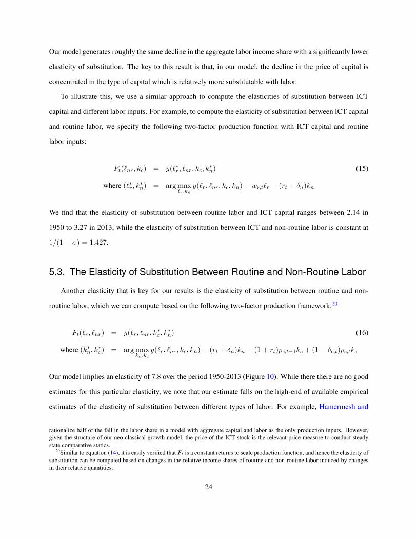
To illustrate this, we use a similar approach to compute the elasticities of substitution between ICT
capital and different labor inputs. For example, to compute the elasticity of substitution between ICT capital
and routine labor, we specify the following two-factor production function with ICT capital and routine
labor inputs:
Ft(`nr, kc) = y(`∗r , `nr, kc, k∗n) (15)
where (`∗r , k∗n) = argmax
`r,kny(`r, `nr, kc, kn)− wr,t`r − (rt + δn)kn
We find that the elasticity of substitution between routine labor and ICT capital ranges between 2.14 in
1950 to 3.27 in 2013, while the elasticity of substitution between ICT and non-routine labor is constant at
1/(1− σ) = 1.427.
5.3. The Elasticity of Substitution Between Routine and Non-Routine Labor
Another elasticity that is key for our results is the elasticity of substitution between routine and non-
routine labor, which we can compute based on the following two-factor production framework:20
Ft(`r, `nr) = y(`r, `nr, k∗c , k∗n) (16)
where (k∗n, k∗c ) = argmax
kn,kcy(`r, `nr, kc, kn)− (rt + δn)kn − (1 + rt)pc,t−1kc + (1− δc,t)pc,tkc
Our model implies an elasticity of 7.8 over the period 1950-2013 (Figure 10). While there there are no good
estimates for this particular elasticity, we note that our estimate falls on the high-end of available empirical
estimates of the elasticity of substitution between different types of labor. For example, Hamermesh and
rationalize half of the fall in the labor share in a model with aggregate capital and labor as the only production inputs. However,given the structure of our neo-classical growth model, the price of the ICT stock is the relevant price measure to conduct steadystate comparative statics.
20Similar to equation (14), it is easily verified that Ft is a constant returns to scale production function, and hence the elasticity ofsubstitution can be computed based on changes in the relative income shares of routine and non-routine labor induced by changesin their relative quantities.
24

Figure 10: Calibrated Elasticity of Substitution Between Routine and Non-Routine Labor
1950 1960 1970 1980 1990 2000 2010 2020
Year
7.75
7.8
7.85
7.9
7.95
8
8.05
Ela
sticity O
f S
ub
stitu
tio
n
EOS(R,X) = 1/(1-θ)
EOS(R,NR)
Notes: The figure plots calibrated elasticities of substitution. The EOS betweenR and NR workers is based on the two-factor production function (16). Numer-ical values for this elasticity are computed for each point along our our baselinesimulation.
Grant (1979) survey an older literature that estimates the EOS between various “types” of workers (including
production vs. non-production, educated vs. non-educated, etc.) which range from marginally negative to as
large as 12. Two recent papers estimate elasticity parameters that are conceptually very close to ours and fall
at the lower end of this range: Goos, Manning and Salomons (2014) estimate an EOS between a continuum
of tasks with differing “routine intensity” of 0.9, while Lee and Shin (2017) find an EOS between “workers”
and “managers” of 0.341.
Our calibration of a high EOS is a result of attributing the entire decline in the routine labor income
share to changes in relative factor supplies. To illustrate this point, consider an alternative specification of
the production structure, in which the production parameter η, which governs the demand for routine labor,
evolves exogenously according to:ηt
1− ηt= a exp(ρt) (17)
for some ρ and a > 0. In our baseline calibration, ρ = 0 and η is time invariant. An alternative parameteri-
25

zation of ρ < 0 implies an exogenous decrease in the relative demand for routine labor, which is unrelated
to the increase in the ICT capital stock. Under these assumptions, equation (7) can then be rewritten as
ln
(sr,tsz,t
)= a+ ρt+ θ ln
(`r,tzt
)(18)
Equation (18) implies that any given trend in relative income shares can be accounted for by different
combinations of θ and ρ. Moreover, a lower θ (and hence a lower elasticity of substitution between routine
and non-routine labor) can be made consistent with observed trends when combined with a lower ρ.
As an illustration, Figure 11 presents the simulation results obtained from a calibration that targets
EOS(`r, `nr) = 1/3, very close to the estimate of Lee and Shin (2017).21 Here, the counterfactual sim-
ulation is one in which both the price of ICT capital and its depreciation rate are held fixed, but η evolves
exogenously according to the law of motion (17). This alternative calibration attributes a smaller share of the
declining labor income share to the declining price of ICT capital. While the baseline simulation continues
to imply a 3.5pp decline in the labor income share between steady states, part of this decline is attributed to
the exogenous decline in η. Note that a decline in the demand for routine labor is equivalent to an increase
in the demand for z, and hence for ICT capital. In this environment, automation is driven both by cheaper
ICT capital and by an exogenous process that increases the demand for z.
A less-than-unitary elasticity of substitution between routine and non-routine labor implies that the fall
in the ICT price increases the income share of routine labor, while reducing the income share of non-routine
labor (Panel C of Figure 11). This is due to complementarity: an increase in the quantity of z relative to
`r increases the relative income share of `r. Of course, other specifications of the aggregate production
function may alter these comparative statics while maintaining the elasticity of substitution between routine
and non-routine labor.
Given the wide range of estimates for the EOS discussed above, Table 6 illustrates the implications for
the aggregate labor share over the period 1950-2013 under alternative assumptions about the EOS. For all
calibrations, the model accounts for approximately half of the measured 6.5pp decline in the aggregate labor
share over this period. The table shows that ICT accounts for as much as 60% of this decline, even with an
21To match an average elasticity of substitution between routine and non-routine labor of 1/3, we calibrate θ = −2.0303,a = 0.8775 and ρ = −0.075.
26
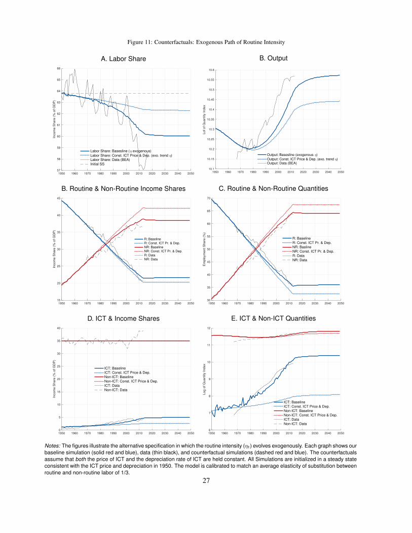
Figure 11: Counterfactuals: Exogenous Path of Routine Intensity
A. Labor Share B. Output
1950 1960 1970 1980 1990 2000 2010 2020 2030 2040 205057
58
59
60
61
62
63
64
65
66
Inco
me
Sh
are
(%
of
GD
P)
Labor Share: Basesline (η exogenous)
Labor Share: Const. ICT Price & Dep. (exo. trend η)Labor Share: Data (BEA)
Initial SS
1950 1960 1970 1980 1990 2000 2010 2020 2030 2040 205010.1
10.15
10.2
10.25
10.3
10.35
10.4
10.45
10.5
10.55
10.6
Lo
f o
f Q
ua
ntity
In
de
x
Output: Basesline (exogenous η)
Output: Const. ICT Price & Dep. (exo. trend η)Output: Data (BEA)
B. Routine & Non-Routine Income Shares C. Routine & Non-Routine Quantities
1950 1960 1970 1980 1990 2000 2010 2020 2030 2040 205015
20
25
30
35
40
45
Inco
me
Sh
are
(%
of
GD
P)
R: Baseline
R: Const. ICT Pr. & Dep.
NR: Baseline
NR: Const. ICT Pr. & Dep.
R: Data
NR: Data
1950 1960 1970 1980 1990 2000 2010 2020 2030 2040 205030
35
40
45
50
55
60
65
70
Em
plo
ym
en
t S
ha
re (
%)
R: Baseline
R: Const. ICT Pr. & Dep.
NR: Basline
NR: Const. ICT Pr. & Dep.
R: Data
NR: Data
D. ICT & Income Shares E. ICT & Non-ICT Quantities
1950 1960 1970 1980 1990 2000 2010 2020 2030 2040 20500
5
10
15
20
25
30
35
40
Inco
me
Sh
are
(%
of
GD
P)
ICT: Baseline
ICT: Const. ICT Price & Dep.
Non-ICT: Baseline
Non-ICT: Const. ICT Price & Dep.
ICT: Data
Non-ICT: Data
1950 1960 1970 1980 1990 2000 2010 2020 2030 2040 20506
7
8
9
10
11
12
Lo
g o
f Q
ua
ntity
In
de
x
ICT: Baseline
ICT: Const. ICT Price & Dep.
Non-ICT: Baseline
Non-ICT: Const. ICT Price & Dep.
ICT: Data
Non-ICT: Data
Notes: The figures illustrate the alternative specification in which the routine intensity (ηt) evolves exogenously. Each graph shows ourbaseline simulation (solid red and blue), data (thin black), and counterfactual simulations (dashed red and blue). The counterfactualsassume that both the price of ICT and the depreciation rate of ICT are held constant. All Simulations are initialized in a steady stateconsistent with the ICT price and depreciation in 1950. The model is calibrated to match an average elasticity of substitution betweenroutine and non-routine labor of 1/3.
27

Table 6: Model Predicted Decline in the Labor Share (1950-2013)
Perc. Point Decline in the Labor Share (1950-2013)
Calibrated Parameters due to ICT
(1) (2) (3) (4) (5) (6) (7) (8)EOS(`r, `nr) θ a ρ ∆sL due to trend in η pp % of total
0.25 -3.000 1.1240 -0.0999 -3.47 -1.43 -2.05 58.910.33 -2.030 0.8775 -0.0750 -3.43 -1.40 -2.03 59.260.70 -0.429 0.4704 -0.0339 -3.31 -1.30 -2.01 60.680.90 -0.111 0.3898 -0.0258 -3.28 -1.27 -2.02 61.401.50 0.333 0.2768 -0.0144 -3.21 -1.17 -2.04 63.623.00 0.667 0.1921 -0.0058 -3.10 -0.95 -2.15 69.475.00 0.800 0.1582 -0.0024 -2.98 -0.65 -2.33 78.107.00 0.857 0.1437 -0.0009 -2.86 -0.35 -2.51 87.658.00 0.875 0.1391 -0.0005 -2.81 -0.20 -2.61 92.74
Notes: The table reports the percentage point decline in the aggregate labor share over the period 1950-2013. Column 1 reports alternative targets for EOS(`r, `nr) and Colums 2-4 report the correspondingcalibrated parameter values. Column 5 reports the predicted, percentage point decline in the labor sharedue to the combined impact of an exogenous trend in η as well as a changing ICT price and depreciation.Columns 6-8 decompose the overall decline from Column 5 into the portion due to the exogenous trendin η and the portion due to ICT accumulation. The final decomposition is derived from the counterfactualpaths as displayed in Figure 11 for the case of EOS(`r, `nr)=1/3.
elasticity of substitution that is as low as 1/4.
This exercise illustrates that a lower elasticity of substitution between routine and non-routine labor can
be made consistent with observed trends if there is an exogenous decline in the demand for routine work.
Given that attributing the entire transformation in labor income to changes in factor supplies necessitates
a very high elasticity of substitution between routine and non-routine labor, we conclude that additional
factors are likely contributing to the decline in the routine labor income share.
6. Concluding Remarks
The discussion on the social costs and benefits of automation can roughly be divided into two issues: its
effects on aggregate consumption and its distributional implications. The general consensus is that, while
there is likely a positive effect on aggregate consumption, there are some adverse distributional implications.
This paper sets out to inform this discussion in two ways. First, we document changes in the income
shares of different factors of production in order to comment on the potential distributional implications of
ICT. Our analysis suggests that the income share of ICT capital has increased by about 3pp and that this
increase has come at the expense of labor income. Within labor, we document a large shift in the distribution
28

of income between routine and non-routine occupations. However, our analysis suggests that it is unlikely
that the accumulation of ICT capital is the sole driver of this shift. In particular, given the small income
share of ICT capital, the large simultaneous increases in the relative employment in non-routine occupations
and the relative pay for non-routine work are difficult to reconcile with a standard production function with
time invariant parameters. Doing so requires a very high elasticity of substitution between routine and
non-routine labor, which is likely unrealistic.
Second, our analysis informs the discussion by providing an upper bound on the aggregate welfare
gains from automation. We find that, in a representative agent model, the declining price of ICT capital
generates an aggregate welfare gain of about 4%. By construction, this estimate ignores any potential
adverse distributional implications, as well as any costs associated with reallocating labor from routine to
non-routine occupations. Hence, a 4% welfare gain should be interpreted as an upper bound.
References
Acemoglu D, Autor D. 2011. Skills, Tasks and Technologies: Implications for Employment and Earnings, volume 4 of Handbook of Labor
Economics, chapter 12. Elsevier, 1043–1171.
URL http://ideas.repec.org/h/eee/labchp/5-12.html
Acemoglu D, Autor D, Dorn D, Hanson GH, Price B. 2014. Return of the Solow Paradox? IT, Productivity, and Employment in US Manufacturing.
American Economic Review 104: 394–99.
URL http://ideas.repec.org/a/aea/aecrev/v104y2014i5p394-99.html
Akerman A, Gaarder I, Mogstad M. 2015. The Skill Complementarity of Broadband Internet. The Quarterly Journal of Economics 130: 1781–1824.
URL https://ideas.repec.org/a/oup/qjecon/v130y2015i4p1781-1824.html
Alvarez-Cuadrado F, Long NV, Poschke M. 2015. Capital-Labor Substitution, Structural Change and the Labor Income Share. IZA Discussion
Papers 8941, Institute for the Study of Labor (IZA).
URL https://ideas.repec.org/p/iza/izadps/dp8941.html
Antras P. 2004. Is the u.s. aggregate production function cobb-douglas? new estimates of the elasticity of substitution. The B.E. Journal of
Macroeconomics 4: 1–36.
URL http://ideas.repec.org/a/bpj/bejmac/vcontributions.4y2004i1n4.html
Autor D, Dorn D, Hanson GH. 2013. Untangling Trade and Technology: Evidence from Local Labor Markets. IZA Discussion Papers 7329,
Institute for the Study of Labor (IZA).
URL http://ideas.repec.org/p/iza/izadps/dp7329.html
Autor DH, Dorn D. 2013. The growth of low-skill service jobs and the polarization of the us labor market. American Economic Review 103:
29

1553–97.
URL http://ideas.repec.org/a/aea/aecrev/v103y2013i5p1553-97.html
Autor DH, Levy F, Murnane RJ. 2003. The skill content of recent technological change: An empirical exploration. The Quarterly Journal of
Economics 118: 1279–1333.
URL http://ideas.repec.org/a/tpr/qjecon/v118y2003i4p1279-1333.html
Basu S, Fernald JG, Oulton N, Srinivasan S. 2003. The Case of the Missing Productivity Growth: Or, Does Information Technology Explain why
Productivity Accelerated in the US but not the UK? NBER Working Papers 10010, National Bureau of Economic Research, Inc.
URL http://ideas.repec.org/p/nbr/nberwo/10010.html
Berndt ER. 1976. Reconciling Alternative Estimates of the Elasticity of Substitution. The Review of Economics and Statistics 58: 59–68.
URL https://ideas.repec.org/a/tpr/restat/v58y1976i1p59-68.html
Blackorby C, Russell RR. 1989. Will the Real Elasticity of Substitution Please Stand Up? (A Comparison of the Allen/Uzawa and Morishima
Elasticities). American Economic Review 79: 882–888.
URL https://ideas.repec.org/a/aea/aecrev/v79y1989i4p882-88.html
Blanchard OJ. 1997. The medium run. Brookings Papers on Economic Activity 1997: 89–158.
Bridgman B. 2014. Is Labor’s Loss Capital’s Gain? Gross versus Net Labor Shares. BEA Working Papers 0114, Bureau of Economic Analysis.
URL http://ideas.repec.org/p/bea/wpaper/0114.html
Brynjolfsson E, Hitt LM. 2003. Computing productivity: Firm-level evidence. The Review of Economics and Statistics 85: 793–808.
URL http://ideas.repec.org/a/tpr/restat/v85y2003i4p793-808.html
Caballero RJ, Hammour ML. 1998. Jobless growth: appropriability, factor substitution, and unemployment. Carnegie-Rochester Conference Series
on Public Policy 48: 51 – 94. ISSN 0167-2231.
URL http://www.sciencedirect.com/science/article/pii/S0167223198000165
Caselli F, Feyrer J. 2007. The marginal product of capital. The Quarterly Journal of Economics 122: 535–568.
URL http://ideas.repec.org/a/tpr/qjecon/v122y2007i2p535-568.html
Champagne J, Kurmann A, Stewart J. 2017. Reconciling the divergence in aggregate u.s. wage series. Working Paper.
URL https://sites.google.com/site/julienjchampagnephd/CESpaper_March2017.pdf
Christensen LR, Jorgenson DW. 1969. The measurement of us real capital input, 1929–1967. Review of Income and Wealth 15: 293–320.
Colecchia A, Schreyer P. 2002. ICT Investment and Economic Growth in the 1990s: Is the United States a Unique Case? A Comparative Study of
Nine OECD Countries. Review of Economic Dynamics 5: 408–442.
URL http://ideas.repec.org/a/red/issued/v5y2002i2p408-442.html
Cortes GM, Jaimovich N, Nekarda CJ, Siu HE. 2014. The micro and macro of disappearing routine jobs: A flows approach. Working Paper 20307,
National Bureau of Economic Research.
URL http://www.nber.org/papers/w20307
Dorn D. 2009. Essays on inequality, spatial interaction, and the demand for skills. Dissertation 3613, University of St. Gallen.
30

Eden M, Gaggl P. 2015. Do poor countries really need more IT ? the role of relative prices and industrial composition. Policy Research Working
Paper Series 7352, The World Bank.
URL http://ideas.repec.org/p/wbk/wbrwps/7352.html
Elsby MW, Hobijn B, Sahin A. 2013. The decline of the us labor share. Brookings Papers on Economic Activity .
Gaggl P, Wright GC. 2017. A Short-Run View of What Computers Do: Evidence from a UK Tax Incentive. American Economic Journal: Applied
Economics 9: 262–294.
URL https://ideas.repec.org/a/aea/aejapp/v9y2017i3p262-94.html
Glover AS, Short JM. 2017. Can capital deepening explain the global decline in labor’s share? SSRN working paper.
URL https://ssrn.com/abstract=2970250
Goos M, Manning A, Salomons A. 2014. Explaining job polarization: Routine-biased technological change and offshoring. American Economic
Review 104: 2509–26.
URL http://www.aeaweb.org/articles?id=10.1257/aer.104.8.2509
Guvenen F. 2006. Reconciling conflicting evidence on the elasticity of intertemporal substitution: A macroeconomic perspective. Journal of
Monetary Economics 53: 1451–1472.
URL http://ideas.repec.org/a/eee/moneco/v53y2006i7p1451-1472.html
Hall RE, Jorgenson DW. 1967. Tax policy and investment behavior. The American Economic Review 57: pp. 391–414. ISSN 00028282.
URL http://www.jstor.org/stable/1812110
Hamermesh D, Grant J. 1979. Econometric studies of labor-labor substitution and their implications for policy. Journal of Human Resources 14:
543–562.
URL http://EconPapers.repec.org/RePEc:uwp:jhriss:v:14:y:1979:i:4:p:543-562
Herrendorf B, Herrington C, Valentinyi A. 2015. Sectoral Technology and Structural Transformation. American Economic Journal: Macroeco-
nomics 7: 104–33.
URL https://ideas.repec.org/a/aea/aejmac/v7y2015i4p104-33.html
Jaimovich N, Pruitt S, Siu HE. 2013. The Demand for Youth: Explaining Age Differences in the Volatility of Hours. American Economic Review
103: 3022–44.
URL https://ideas.repec.org/a/aea/aecrev/v103y2013i7p3022-44.html
Jorgenson DW. 1995. Productivity: Postwar US economic growth, volume 1. Mit Press.
Jorgenson DW, Vu K. 2007. Information Technology and the World Growth Resurgence. German Economic Review 8: 125–145.
URL http://ideas.repec.org/a/bla/germec/v8y2007ip125-145.html
Karabarbounis L, Neiman B. 2014. The global decline of the labor share. The Quarterly Journal of Economics 129: 61–103.
URL http://qje.oxfordjournals.org/content/129/1/61.abstract
Klump R, McAdam P, Willman A. 2007. Factor Substitution and Factor-Augmenting Technical Progress in the United States: A Normalized
Supply-Side System Approach. The Review of Economics and Statistics 89: 183–192.
URL https://ideas.repec.org/a/tpr/restat/v89y2007i1p183-192.html
31

Krusell P, Ohanian LE, Rıos-Rull JV, Violante GL. 2000. Capital-Skill Complementarity and Inequality: A Macroeconomic Analysis. Econometrica
68: 1029–1054.
URL http://ideas.repec.org/a/ecm/emetrp/v68y2000i5p1029-1054.html
Lee SY, Shin Y. 2017. Horizontal and vertical polarization: Task-specific technological change in a multi-sector economy. Working Paper 23283,
National Bureau of Economic Research.
URL http://www.nber.org/papers/w23283
Miyagiwa K, Papageorgiou C. 2007. Endogenous aggregate elasticity of substitution. Journal of Economic Dynamics and Control 31: 2899–2919.
URL https://ideas.repec.org/a/eee/dyncon/v31y2007i9p2899-2919.html
Oberfield E, Raval D. 2014. Micro Data and Macro Technology. NBER Working Papers 20452, National Bureau of Economic Research, Inc.
URL https://ideas.repec.org/p/nbr/nberwo/20452.html
O’Mahony M, Van Ark B. 2003. EU productivity and competitiveness: an industry perspective: can Europe resume the catching-up process?
Office for Official Publications of the European Communities Luxembourg.
Piketty T. 2014. Capital in the Twenty-First Century. Harvard University Press. ISBN 9780674369559.
URL https://books.google.com/books?id=J222AgAAQBAJ
Piketty T, Saez E. 2003. Income inequality in the united states, 1913-1998. The Quarterly Journal of Economics 118: 1–39.
URL http://ideas.repec.org/a/tpr/qjecon/v118y2003i1p1-39.html
Rognlie M. 2015. Deciphering the fall and rise in the net capital share. In Brookings Papers on Economic Activity. Conference Draft.
URL http://www.brookings.edu/˜/media/projects/bpea/spring-2015/2015a_rognlie.pdf
Ruggles S, Alexander JT, Genadek K, Goeken R, Schroeder MB, Sobek M. 2010. Integrated public use microdata series: Version 5.0 [machine-
readable database]. Technical report, University of Minnesota, Minneapolis.
URL https://cps.ipums.org/cps/
Solow RM. 1957. Technical change and the aggregate production function. The Review of Economics and Statistics 39: 312–320.
Stiroh KJ. 2002. Information Technology and the U.S. Productivity Revival: What Do the Industry Data Say? American Economic Review 92:
1559–1576.
URL https://ideas.repec.org/a/aea/aecrev/v92y2002i5p1559-1576.html
vom Lehn C. 2015. Labor Market Polarization, the Decline of Routine Work, and Technological Change: A Quantitative Evaluation. 2015 Meeting
Papers 151, Society for Economic Dynamics.
URL http://ideas.repec.org/p/red/sed015/151.html
32

Appendix A. Classification of ICT and Non-ICT Assets
Table A.7: ICT AssetsShare of Aggregate Capital (%) Average Growth in Share (%)
ICT Assets 1960-1980 1980-2000 2000-2013 1960-1980 1980-2000 2000-2013
EP20: Communications 2.73 3.91 3.39 2.87 1.78 -2.63ENS3: Own account software 0.24 0.75 1.56 27.26 6.68 2.58ENS2: Custom software 0.11 0.61 1.40 34.82 8.49 2.06EP34: Nonelectro medical instruments 0.35 0.76 1.08 4.87 2.97 2.30EP36: Nonmedical instruments 0.51 0.92 0.92 0.62 2.41 -1.08ENS1: Prepackaged software 0.02 0.33 0.83 32.28 14.63 -1.04EP35: Electro medical instruments 0.11 0.36 0.66 7.25 3.43 4.28EP1B: PCs 0.00 0.31 0.45 12.12 0.96RD23: Semiconductor and other component manufacturing 0.05 0.23 0.43 6.58 8.21 2.75RD22: Communications equipment manufacturing 0.26 0.21 0.27 3.27 0.89 0.24EP31: Photocopy and related equipment 0.53 0.75 0.26 6.75 -2.11 -7.70EP1A: Mainframes 0.19 0.36 0.24 24.00 1.91 -4.97EP1H: System integrators 0.00 0.03 0.23 42.85 3.45RD24: Navigational and other instruments manufacturing 0.05 0.19 0.22 3.20 5.78 -1.59EP1D: Printers 0.07 0.22 0.19 20.75 7.20 -9.76EP1E: Terminals 0.02 0.14 0.16 71.14 5.48 -4.62EP1G: Storage devices 0.00 0.17 0.12 7.55 -9.55EP12: Office and accounting equipment 0.48 0.32 0.12 -3.09 -5.00 -6.13RD40: Software publishers 0.00 0.05 0.09 16.91 -1.13RD21: Computers and peripheral equipment manufacturing 0.16 0.09 0.07 3.68 -3.07 -0.60RD25: Other computer and electronic manufacturing, n.e.c. 0.01 0.01 0.02 0.91 3.24 -0.34EP1C: DASDs 0.09 0.13 0.00 30.38 -36.26 -78.36EP1F: Tape drives 0.06 0.03 0.00 22.77 -40.33 -186.06
Notes: The data are drawn from the BEA’s detailed fixed asset accounts. ICT assets are defined as BEA asset codes startingwith EP, EN, RD2, or RD4. Notice that the EP category incorporates two assets that are strictly speaking likely not ICT: EP34 andEP36. Our results do not critically hinge on these two assets and we therefore stick with the more standard BEA aggregation ofEP. Assets are ranked by their average share in aggregate capital during 2000-2013. The share of aggregate captial is the value ofeach individual asset, as estimated by the BEA at current cost, as a fraction of the value of all assets in Tables A.7 and A.8. Panel Areports averages of these shares for three time periods. Panel B reports the average annual growth in these shares over same threetime periods.
33

Table A.8: Non-ICT AssetsA. Average Share of Aggregate Capital (%) B. Average Growth in Share (%)
Non-ICT Assets 1960-1980 1980-2000 2000-2013 1960-1980 1980-2000 2000-2013SOO1: Office 4.75 6.99 8.28 1.59 2.14 0.12SI00: Manufacturing 8.27 8.07 6.96 0.22 -0.44 -1.39SM01: Petroleum and natural gas 3.91 3.63 5.20 0.12 -2.30 6.54SU30: Electric 6.44 5.48 4.73 -0.18 -1.79 0.89SC03: Multimerchandise shopping 2.21 2.77 3.05 1.46 0.69 0.59EI50: General industrial equipment 3.42 3.40 2.95 0.32 -0.60 -0.75SB31: Hospitals 1.70 2.52 2.86 3.69 1.06 0.51SU20: Communication 2.80 2.51 2.66 0.70 -1.09 1.79SC02: Other commercial 1.55 2.00 2.47 1.43 1.41 0.38SB41: Lodging 1.58 1.83 2.32 1.40 1.76 0.47EI60: Electric transmission and distribution 2.87 2.50 2.16 -0.79 -0.64 -0.21EI40: Special industrial machinery 2.63 2.52 1.95 -0.36 -0.07 -3.33SB20: Educational and vocational 1.56 1.36 1.92 -0.26 0.68 2.78SC01: Warehouses 1.18 1.40 1.89 0.54 1.57 1.03ET30: Aircraft 1.17 1.59 1.79 5.36 0.94 0.37EO80: Other 1.09 1.44 1.75 2.30 1.18 0.71EO12: Other furniture 1.37 1.67 1.74 -0.45 1.68 -1.35SB42: Amusement and recreation 1.84 1.67 1.70 -0.46 0.54 -1.44SN00: Farm 3.48 2.46 1.69 -0.63 -2.66 -2.11RD11: Pharmaceutical and medicine manufacturing 0.23 0.65 1.68 4.70 6.63 5.22SU40: Gas 2.70 1.89 1.66 -1.66 -1.72 0.35SC04: Food and beverage establishments 1.19 1.51 1.58 1.47 0.84 -0.51SB10: Religious 2.11 1.57 1.51 -0.70 -0.73 -0.82EI30: Metalworking machinery 2.32 2.10 1.49 0.46 -1.25 -3.31ET11: Light trucks (including utility vehicles) 0.93 1.05 1.42 0.45 2.48 -2.56RDOM: Other manufacturing 1.47 1.50 1.19 0.00 0.04 -1.13ET20: Autos 1.80 1.67 1.14 -1.79 -0.33 -4.27ET12: Other trucks, buses and truck trailers 1.59 1.46 1.02 0.54 -1.43 -3.04SU11: Other railroad 4.14 1.86 0.97 -4.62 -3.94 -3.77SU12: Track replacement 2.66 1.39 0.97 -4.22 -2.69 -1.34SOO2: Medical buildings 0.57 0.83 0.95 1.55 1.90 0.25EO40: Other construction machinery 1.16 1.02 0.94 1.79 -2.11 1.37AE10: Theatrical movies 0.97 0.67 0.86 -4.28 2.37 0.00AE20: Long-lived television programs 0.69 0.79 0.86 0.39 1.91 -0.55EO60: Service industry machinery 1.14 0.94 0.85 -1.61 -0.49 0.00EI12: Other fabricated metals 1.42 1.20 0.75 0.83 -3.88 -0.19RD80: All other nonmanufacturing, n.e.c. 0.09 0.75 0.72 3.04 8.28 -3.34SB32: Special care 0.41 0.62 0.71 3.70 1.59 -0.74ET50: Railroad equipment 2.12 1.09 0.66 -1.97 -4.52 -0.75EO30: Other agricultural machinery 1.58 1.11 0.63 0.61 -4.71 -0.74EI21: Steam engines 0.75 0.57 0.46 0.16 -3.01 0.43SU50: Petroleum pipelines 0.95 0.57 0.45 -2.76 -3.29 1.69AE30: Books 0.40 0.42 0.43 -0.37 1.02 -0.54ET40: Ships and boats 0.92 0.68 0.40 -0.91 -3.72 -1.18RD92: Other nonprofit institutions 0.22 0.35 0.38 3.94 2.25 0.23RD31: Motor vehicles and parts manufacturing 0.40 0.44 0.36 0.45 0.79 -4.90SM02: Mining 0.31 0.40 0.35 2.12 -1.30 1.93RD12: Chemical manufacturing, ex. pharma and med 0.59 0.47 0.34 0.04 -0.98 -1.58EO50: Mining and oilfield machinery 0.54 0.39 0.31 0.73 -5.74 7.21SO01: Water supply 0.23 0.28 0.28 0.22 1.25 -0.60EO21: Farm tractors 0.69 0.44 0.28 -0.08 -4.65 -0.28SO02: Sewage and waste disposal 0.24 0.29 0.28 0.26 1.16 -1.21RD32: Aerospace products and parts manufacturing 0.33 0.41 0.25 2.09 -0.28 -2.54AE40: Music 0.21 0.20 0.20 0.14 1.37 -4.21RD70: Scientific research and development services 0.00 0.06 0.19 11.29 4.20SO04: Highway and conservation and development 0.15 0.18 0.18 0.27 1.20 -0.44SB43: Air transportation 0.15 0.15 0.17 0.74 1.03 -0.69AE50: Other entertainment originals 0.18 0.17 0.17 -1.71 1.53 -2.58SU60: Wind and solar 0.00 0.01 0.16 12.44 25.22EO72: Other electrical 0.12 0.19 0.14 2.74 -0.20 -1.74SO03: Public safety 0.14 0.10 0.11 -0.96 0.17 -0.55RD60: Computer systems design and related services 0.00 0.03 0.11 22.31 2.68EO11: Household furniture 0.16 0.13 0.10 0.19 -2.30 -1.38EO22: Construction tractors 0.28 0.18 0.09 0.39 -5.15 -3.98EI22: Internal combustion engines 0.09 0.08 0.08 -0.80 -1.19 0.43SB44: Local transit structures 0.51 0.17 0.07 -6.06 -5.15 -4.84EI11: Nuclear fuel 0.03 0.10 0.06 27.52 -3.93 -1.86RD91: Private universities and colleges 0.03 0.04 0.06 0.95 2.71 3.68SOMO: Mobile structures 0.05 0.07 0.05 0.35 1.29 -3.77SB46: Other land transportation 0.04 0.03 0.05 -0.72 1.04 2.80RD50: Financial and real estate services 0.00 0.02 0.05 22.33 -0.88EO71: Household appliances 0.09 0.05 0.03 -2.09 -4.08 -2.35SB45: Other transportation 0.02 0.02 0.02 -0.70 0.56 -0.71Notes: The data are drawn from the BEA’s detailed fixed asset accounts. Assets are ranked by their average share in aggregatecapital during 2000-2013. The share of aggregate captial is the value of each individual asset, as estimated by the BEA at currentcost, as a fraction of the value of all assets in Tables A.7 and A.8. Panel A reports averages of these shares for three time periods.Panel B reports the average annual growth in these shares over same three time periods.
34

Appendix B. Construction of Capital Income Shares
This appendix outlines our approach to measure income shares directly from the BEA’s nominal current
cost values of detailed asset categories. As discussed in Section 2, our measurement exercise relies on two
assumptions: First, no-arbitrage in capital markets requires the return net of depreciation (2) to be equalized
across all types of capital, which can be written more compactly as
(1 + πi,t)Ri,tPi,t
+ CGi,t = 1 + rt (B.1)
where (1 + πi,t) ≡ Pi,t+1/Pi,t captures price inflation and CGi,t = (1 + πi,t)(1− δt) are capital gains (net
of depreciation) for capital of type i.
Second, we impose constant returns to scale in aggregate production (equation (1)), and thus the follow-
ing condition must hold:
sK,tPtYt =∑i∈I
Ri,tKi,t (B.2)
where sK,t is a measure of the income share paid to reproducible capital. Equations (B.1) and (B.2) imply
the following expressions for the relative price adjusted rental rates for each capital type i = {c, n}:
PR c,t =Rc,tPc,t
=Pn,tKn,t
PtKt
(CGn,t − CGc,t) + (1 + πn,t)sK,tPtYt
PtKt
(B.3)
PRn,t =Rn,tPn,t
=Pc,tKc,t
PtKt
(CGc,t − CGn,t) + (1 + πc,t)sK,tPtYt
PtKt
(B.4)
where PtKt ≡ (1 + πn,t)Pc,tKc,t + (1 + πc,t)Pn,tKn,t. Based on (B.3) and (B.4) we then compute the
income shares for each type of capital as
sc,t = PR c,tPc,tKc,t
PtYt(B.5)
sn,t = PRn,tPn,tKn,t
PtYt(B.6)
35
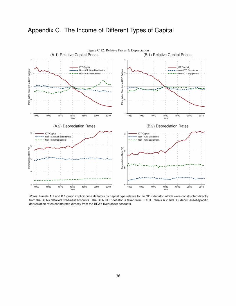
Appendix C. The Income of Different Types of Capital
Figure C.12: Relative Prices & Depreciation(A.1) Relative Capital Prices (B.1) Relative Capital Prices
0.5
11.5
2P
rice Index R
ela
tive to G
DP
Deflato
r
1950 1960 1970 1980 1990 2000 2010Year
ICT Capital
Non−ICT: Non Residential
Non−ICT: Residential
0.5
11.5
2P
rice Index R
ela
tive to G
DP
Deflato
r
1950 1960 1970 1980 1990 2000 2010Year
ICT Capital
Non−ICT: Structures
Non−ICT: Equipment
(A.2) Depreciation Rates (B.2) Depreciation Rates
05
10
15
20
Depre
cia
tion R
ate
(%
)
1950 1960 1970 1980 1990 2000 2010Year
ICT Capital
Non−ICT: Non Residential
Non−ICT: Residential
510
15
20
Depre
cia
tion R
ate
(%
)
1950 1960 1970 1980 1990 2000 2010Year
ICT Capital
Non−ICT: Structures
Non−ICT: Equipment
Notes: Panels A.1 and B.1 graph implicit price deflators by capital type relative to the GDP deflator, which were constructed directlyfrom the BEA’s detailed fixed-asst accounts. The BEA GDP deflator is taken from FRED. Panels A.2 and B.2 depict asset-specificdepreciation rates constructed directly from the BEA’s fixed asset accounts.
36

Figure C.13: Capital’s Income Share(A) Equipment vs. Structures (B) Residential vs. Non-Residential
01
02
03
04
0%
In
co
me
Sh
are
1950 1960 1970 1980 1990 2000 2010Year
ICT Share
Non−ICT Share: Structures
Non−ICT Share: Equipment
05
10
15
20
25
30
% I
nco
me
Sh
are
1950 1960 1970 1980 1990 2000 2010
Year
ICT Share
Non−ICT Share: Non−Residential
Non−ICT Share: Residential
Notes: Panel A decomposes the NICT share into equipment and structures. Panel B decomposes the NICT share into residentialand non-residential capital. The computations are based on the methodology described in Section 2 and the underlying data arenominal gross capital stocks and depreciation rates, drawn from the BEA’s detailed fixed asset accounts. The vertical dashed lineindicates the year 2001.
Table C.9: Within Industry Trends in Capital Income Shares
ICT Share Non-ICT Share
(1) (2) (3) (4)
Ann. Trend Growth (%) 3.873*** 3.873*** 0.0692 0.0692(0.327) (0.193) (0.205) (0.0601)
Industry FEs yes yesObservations 1197 1197 1197 1197
Notes: The table shows regressions of 100 times the log ICT and NICT shares ona time trend for an annual panel of 19 broad sectors over the period 1949-2012.Columns 1 and 3 report pooled regressions while columns 2 and 4 condition on acomplete set of fixed effects for 19 broad sectors. Sector specific income sharesare based on the BEA fixed asset accounts and the BEA’s estimates of sectorspecific value added and constructed as in Eden and Gaggl (2015). Standarderrors are HAC robust and significance levels are indicated by * p < 0.1, **p < 0.05, and *** p < 0.01.
37

Appendix D. The Role of Industrial Composition
We construct industry-specific ICT and NICT shares as in Eden and Gaggl (2015) based on the BEA’s
detailed fixed asset accounts. We then estimate the average annual growth rates in these income shares both
with and without industry fixed effects. Table C.9 reports the results.
Appendix E. Comparison with Other ICT Measures
While there are several data sources that provide ICT related statistics, we are not aware of any database
other than the BEA fixed asset accounts, that reports quality adjusted prices and stocks of ICT capital for the
US. However, we are able to construct measures for the ICT share from two alternative data sources, whose
growth patterns are comparable.
First, a direct estimate for the ICT share is provided by the Conference Board’s Total Economy Database
(TED, https://www.conference-board.org/data/economydatabase/) for the period 1990-2016, defining ICT
as “hardware, software and communication equipment”.22 Second, the Groningen Growth and Development
Centre’s (GGDC) industry growth accounting database (IGA, http://www.rug.nl/ggdc/projects/iga) defines
ICT as “software, computers and communications equipment” and reports ICT’s share in total capital com-
pensation at the industry level.23 These industry estimates are available for the period 1979-2003, and in
order to make them comparable to our aggregate numbers, we use data on value added by sector from the
BEA as well as the GGDC’s estimates of industry level labor shares, in order to construct a value added
weighted average of the ICT share across industries. While these two alternative sources do not report the
exact list of tangible and intangible assets included in their definition of ICT hardware, software and com-
munication equipment, the definitions appear broadly consistent with our list of ICT assets reported in Table
A.7. Panel A of Figure E.14 plots the levels of our estimates for the ICT share in comparison to the the two
alternatives.
Unfortunately, the levels of these three measures are difficult to compare directly for several reasons.
First, the GGDC database does not report value added by industry. While the BEA does report value added
22See https://www.conference-board.org/retrievefile.cfm?filename=TED SourcesMethods nov20161.pdf&type=subsite for de-tails.
23See http://www.rug.nl/ggdc/docs/eu productivity and competitiveness.pdf for details.
38

Figure E.14: Alternative ICT Share Measures (TED, GGDC)(A) ICT and NICT Shares (B) ICT Share (normalized)
01
23
45
6In
co
me
Sh
are
(%
of
GD
P)
1940 1960 1980 2000 2020Year
ICT Share (BEA based)
ICT Share (TED)
ICT Share (KLEMS)
02
04
06
08
01
00
Ind
ex (
20
01
=1
00
)
1940 1960 1980 2000 2020Year
ICT Share (BEA FA, normalized)
ICT Share (TED, normalized)
ICT Share (KLEMS, normalized)
Notes: Panel A displays our BEA based measure of the ICT share alongside two alternatives provided directly by the ConferenceBoard’s Total Economy Database (TED) and constrcuted from industry level estimates of ICT capital compensation by the GronigenGrowth and Development Center’s (GGDC) industry growth accounting database (IGA). Since all three datasources use a differentmeasure of the labor share as a baseline to decompose factor compensation, panel B reports the ICT share for all three measuresnormalized to 100 in 2001.
by industry, the industry classification/aggregation is not the same and it is not possible to construct a one-
for-one concordance in order to construct the appropriate industry weights. In part due to this problem, and
in part because the GGDC does not cover all industries, the value added weighted average of the GGDC’s
industry level labor shares does not match the BLS’s measure of the aggregate labor share used in our
calculations. Likewise, the TED database also uses a different measure of the aggregate labor share as a
baseline for their decomposition of factor compensation.
Thus, it is perhaps more meaningful to compare the growth trends of the ICT share. To facilitate this
comparison, Panel B of Figure E.14 reports normalized versions of all three estimates for the ICT share. One
can see that, while the levels in panel A do not match very well, the growth patterns appear very similar.
Given that our analysis is mostly focused on trends, the similarity in growth trajectories is reassuring.
As another alternative, the OECD reports ICT investment as a fraction of total fixed capital formation,
based on the following definition: “information technology equipment (computers and related hardware);
communications equipment; and software. Software includes acquisition of pre-packaged software, cus-
tomized software and software developed in-house” (https://data.oecd.org/ict/ict-investment.htm). Finally,
while the EU KLEMS database reports ICT specific measures for many countries, it does not report ICT
39

and NICT separately for the US (http://www.euklems.net/eukISIC4.shtml).
Appendix F. Alternative Composition Adjusted Labor Inputs
This appendix considers different measures of quality-adjusted routine and non-routine labor that ac-
count for changes in observed worker characteristics. We construct quantity indexes by estimating employ-
ment and wage bills within demographic cells based on the following characteristics:
1. five major occupations groups: Managerial, Professional, and Technical; Sales, and Administrative;
Service; Precision Production, Craft, and Repair; Operatives and Laborers
2. four age groups: 16-19; 20-29; 30-49; 50-99
3. gender: male, female
4. three racial groups: White; Black; Other
5. six education groups: None or preschool; Grades 1-4; Grades 5-8; Grades 9-11/12; High school
degree/some college; 2-Year College or more
6. six major sectors: Mining/Constr.; Manufacturing; Transp./Comm./Oth. Util.; Trade; Finance; Ser-
vice
To construct chain indexes, we would ideally like a balanced panel of “demographic bins”, each with
a total wage bill and a total employment count. However, since the CPS is a survey, we naturally end up
with some empty cells, even if the demographic bins are fairly coarse. In order to deal with this problem
we interpolate any “gaps” in the time series, and extrapolate/interpolate using polynomials at the beginning
and end of the sample.24 The demographic bins were chosen as a middle ground between narrow enough
cells to pick up interesting variation in compositional changes, while at the same time limiting the amount
of imputed values. Equipped with a panel of demographic cells, we then use Fisher’s “ideal” formula (and
1979 as the base year) to construct chained aggregates, analogously to our chain weighted quantity indexes
for ICT and NICT capital.
24Even though we are ultimately interested in long run trends, we require that at least 40% of each time series (for a demographicbin) are actual data points and at most 60% of the series is imputed with a log linear trend. We have checked the robustness ofour results with respect to different cutoffs (including 100% data) and we do not notice much difference for the resulting trends inquantity indexes and implicit price deflators. The main benefit of keeping as many bins as possible is that the aggregate wage billin the balanced panel is almost identical to the one measured in the raw, unrestricted data when we choose our 40% cutoff.
40

Figure F.15: Major Occupations: Employment and Real Wage Growth
A.1 Routine Employment A.2 Non-Routine Employment−
50
05
01
00
% C
ha
ng
e F
rom
19
83
(th
in=
raw
, th
ick=
19
79
wo
rke
r)
1970 1980 1990 2000 2010 2020Year
Admin./Sales.
Production/Craft
Operatives/Laborers
−5
00
50
10
01
50
% C
ha
ng
e F
rom
19
83
(th
in=
raw
, th
ick=
19
79
wo
rke
r)
1970 1980 1990 2000 2010 2020Year
Manag./Prof./Tech.
Service
B.1 Routine Wages B.2 Non-Routine Wages
−2
00
20
40
60
80
% C
ha
ng
e F
rom
19
83
(th
in=
raw
, th
ick=
19
79
wo
rke
r)
1970 1980 1990 2000 2010 2020Year
Sales/Admin.
Production/Craft
Operatives/Laborers
−2
00
20
40
60
80
% C
ha
ng
e F
rom
19
83
(th
in=
raw
, th
ick=
19
79
wo
rke
r)
1970 1980 1990 2000 2010 2020Year
Manag./Prof./Tech.
Service
Notes: Raw data are drawn from the CPS March supplement and shown as thin lines. Chain indexes are shown as thick lines andare constructed for the following demographic cells: 5 major occupations, gender, 3 race groups, 4 age groups, 5 education groups,and 6 industry groups. The base year for the chain indexes is 1979.
The resulting chain indexes for five major occupation groups and their associated implicit price deflators
are displayed as thick lines in Figure F.15. As a reference, raw employment counts and average wages within
each occupation group are illustrated as thin lines in the respective color/pattern. These figures indicate
that part of the increase in both routine and non-routine wages is reflecting changes in the demographic
characteristics of workers, suggesting that part of the measured wage increase should be interpreted as
changes in quantities. This is reflected in upward adjustments of the quantity indexes relative to the raw
employment counts. On the flip-side, the implicit price deflators are adjusted downward relative to average
wages. Taken together, Figures F.15 (five major occupations) and F.16 (routine/non-routine) suggest that
both non-routine wages and the quantity of non-routine labor inputs grew systematically faster than in the
41

Figure F.16: Routine/Non-Routine Occupations: Employment and Real Wages
A.1 Employment Levels A.2 Employment Growth from 19832
04
06
08
01
00
Mill
ion
Wo
rke
rs (
thin
)/1
97
9 W
ork
ers
(th
ick)
1970 1980 1990 2000 2010 2020Year
Non−Routine
Routine
−5
00
50
10
0%
Ch
an
ge
Fro
m 1
98
3 (
thin
=ra
w,
thic
k=
19
79
wo
rke
r)
1970 1980 1990 2000 2010 2020Year
Non−Routine
Routine
B.1 Real Wage Levels B.2 Real Wage Growth from 1983
10
00
01
20
00
14
00
01
60
00
18
00
02
00
00
22
00
0R
ea
l W
ag
e (
thin
=ra
w,
thic
k=
19
79
Wo
rke
r)
1970 1980 1990 2000 2010 2020Year
Non−Routine
Routine
−2
00
20
40
60
% C
ha
ng
e F
rom
19
83
(th
in=
raw
, th
ick=
19
79
Wo
rke
r)
1970 1980 1990 2000 2010 2020Year
Non−Routine
Routine
Notes: Raw data are drawn from the CPS March supplement and shown as thin lines. Chain indexes are shown as thick lines andare constructed for the following demographic cells: 5 major occupations, gender, 3 race groups, 4 age groups, 5 education groups,and 6 industry groups. The base year for the chain indexes is 1979.
routine group.
An alternative way to decompose the routine and non-routine income shares into price and quantity
components is based on cross sectional estimates of the non-routine wage premium (NRP). We estimate the
following cross-sectional regression model separately for each year, t:
lnwi,t = β0,t + β1,tNR i,t + β2,tXi,t + εi,t for t ∈ {1967, . . . , 2013}, (F.1)
where NR i,t is a dummy variable indicating that individual i works a non-routine job in year t and Xi,t
includes a variety of control variables. In particular, we include gender, race, and full-time employment
42
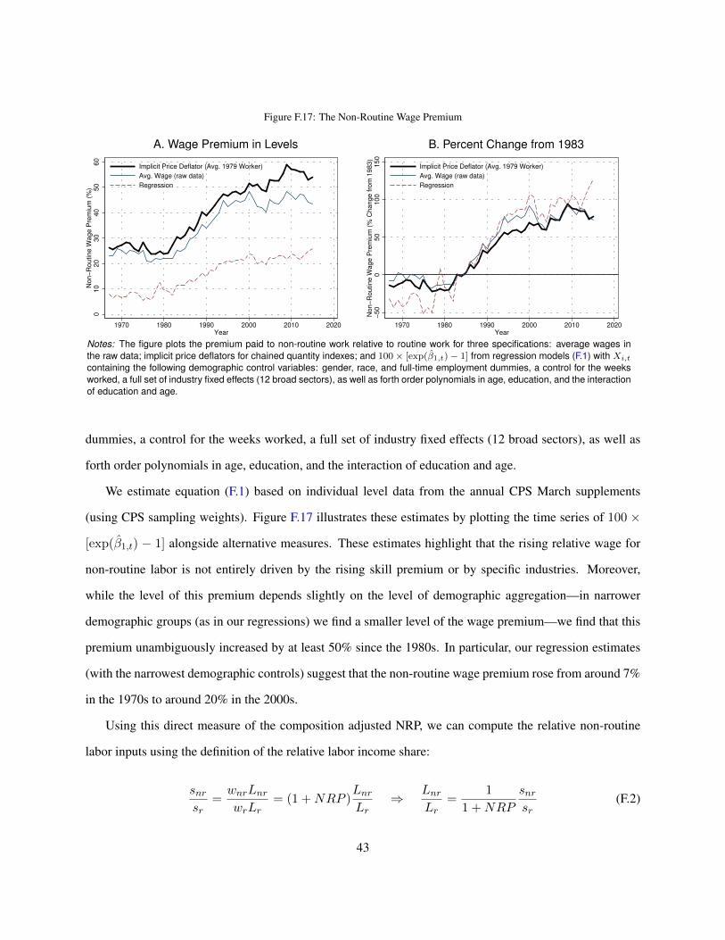
Figure F.17: The Non-Routine Wage Premium
A. Wage Premium in Levels B. Percent Change from 1983
010
20
30
40
50
60
Non−
Routine W
age P
rem
ium
(%
)
1970 1980 1990 2000 2010 2020Year
Implicit Price Deflator (Avg. 1979 Worker)
Avg. Wage (raw data)
Regression
−50
050
100
150
Non−
Routine W
age P
rem
ium
(%
Change fro
m 1
983)
1970 1980 1990 2000 2010 2020Year
Implicit Price Deflator (Avg. 1979 Worker)
Avg. Wage (raw data)
Regression
Notes: The figure plots the premium paid to non-routine work relative to routine work for three specifications: average wages inthe raw data; implicit price deflators for chained quantity indexes; and 100× [exp(β1,t)− 1] from regression models (F.1) with Xi,tcontaining the following demographic control variables: gender, race, and full-time employment dummies, a control for the weeksworked, a full set of industry fixed effects (12 broad sectors), as well as forth order polynomials in age, education, and the interactionof education and age.
dummies, a control for the weeks worked, a full set of industry fixed effects (12 broad sectors), as well as
forth order polynomials in age, education, and the interaction of education and age.
We estimate equation (F.1) based on individual level data from the annual CPS March supplements
(using CPS sampling weights). Figure F.17 illustrates these estimates by plotting the time series of 100 ×
[exp(β1,t) − 1] alongside alternative measures. These estimates highlight that the rising relative wage for
non-routine labor is not entirely driven by the rising skill premium or by specific industries. Moreover,
while the level of this premium depends slightly on the level of demographic aggregation—in narrower
demographic groups (as in our regressions) we find a smaller level of the wage premium—we find that this
premium unambiguously increased by at least 50% since the 1980s. In particular, our regression estimates
(with the narrowest demographic controls) suggest that the non-routine wage premium rose from around 7%
in the 1970s to around 20% in the 2000s.
Using this direct measure of the composition adjusted NRP, we can compute the relative non-routine
labor inputs using the definition of the relative labor income share:
snrsr
=wnrLnrwrLr
= (1 +NRP )LnrLr
⇒ LnrLr
=1
1 +NRP
snrsr
(F.2)
43

Figure F.18: Aggregate Employment Indexes
60
80
10
01
20
14
01
60
Em
plo
ym
en
t (M
illio
n W
ork
ers
)
1970 1980 1990 2000 2010Year
CPS raw counts
Chain Index (1979=Data)
Notes: The figure plots raw CPS MARCH employment counts alonside two ver-sions of aggregate employment indexes: chain indexes that are constructed us-ing the methdology in Appendix F; aggregate employment in units of “referenceworkers” is based on equation (F.1).
Figure F.19: Routine & Non-routine Labor (Relative Quantities & Prices)(A) Relative Quantities (B) NR Wage Premium
50
100
150
200
NR
/R E
mplo
ym
ent (%
of R
Em
plo
ym
ent)
1970 1980 1990 2000 2010Year
Homogeneous Labor (NRP=0)
Composition Adjusted (NRP>0)
Employment Counts
Chain Indexes
010
20
30
40
50
60
Non−
Routine W
age P
rem
ium
(%
)
1970 1980 1990 2000 2010Year
Homogeneous Labor (NRP=0)
Composition Adjusted (NRP>0)
Average Wage
Chain Indexes
Notes: Panel A plots relative employmnet (expressed as percent of routine workers) based on four alternative measurement as-sumptions: the raw data; “effective” employment under the assumption of a homogeneous labor inputs; chain indexes; effective unitsassumingNRP > 0 based on regression model (F.1). Panel B plots the corresponding non-routine wage premium (NRP), defined as100× (wnr/wr − 1), where wnr/wr represents the relative non-routine wage for the four alternative measurement approaches: theratio of average CPS wages; zero NRP by assumption; relative implicit price deflators for chain indexes; exp(β1,t) from regressionmodel (F.1).
44

Quantity indexes for routine and non-routine labor can be obtained from this relation by constructing a
quantity index for aggregate labor (Figure F.18). Figure F.19 compares all relative employment measures
(panel A) and the corresponding non-routine wage premium (panel B).
Appendix G. Alternative Specificaitons for the Composite Input z
In addition to equations (4)-(5), there are two alternative ways to specify a nested CES production
function. The first is in the spirit of Autor and Dorn (2013), who consider the follwing setup:
x = (µzϕ + (1− µ)`ϕnr)1ϕ (G.1)
z = (χkξc + (1− χ)`ξr)1ξ
where µ, χ ∈ [0, 1] and ξ, ϕ ≤ 1. The interpretation is one in which non-routine labor interacts with “routine
inputs” (xr), which can be produced by either routine labor or ICT capital.
For example, a (non-routine) applied economist is more productive if there is more data available; it is
immaterial whether the data is collected by (routine) human surveyors or by an online survey. ICT affects
the productivity of non-routine labor only through increasing the supply of routine inputs, while routine
labor is directly substitutable with ICT.
Table G.10 reports the calibration results based on the specification (G.1). The calibration generates a
value of ϕ > 1 for all versions of labor measurement, inconsistent with the CES framework (which requires
ϕ ≤ 1). Specification (G.1) is therefore inconsistent with the the observed trends in relative prices and
quantities within our fixed CES demand structure.
The second alternative is one in which ICT capital is combined with a CES composite of routine and non-
routine labor. In this setup, the “inner” composite input z is simply a two-factor CES production function in
routine and non-routine labor. Under the assumption of time-invariant parameters, this specification is only
consistent with the assumption of homogeneous labor inputs (NRP=0). To see this, notice that step one in
our calibration procedure for this case can be written as
ln
(snrsr
)= const+ θ ln
(`nr`r
)(G.2)
45

Table G.10: Calibration of Production Parameters
B. Segmented Labor Markets
A. Homogeneous Labor Data Chain Indexes Regressions
(A.1) (A.2) (B.1) (B.2) (B.3) (B.4) (B.5) (B.6)
ln(scsr
)ln
(sxrsnr
)ln
(scsr
)ln
(sxrsnr
)ln
(scsr
)ln
(sxrsnr
)ln
(scsr
)ln
(sxrsnr
)ln (kc/`r) 0.484*** 0.483*** 0.503*** 0.500***
(0.007) (0.007) (0.007) (0.007)ln (z/`nr) 1.242*** 1.944*** 2.037*** 1.656***
(0.009) (0.025) (0.027) (0.017)Constant -6.866*** -0.135*** -6.813*** -0.819*** -6.966*** -0.894*** -6.976*** -0.413***
(0.064) (0.002) (0.063) (0.011) (0.068) (0.012) (0.068) (0.005)
Obs. 47 47 47 47 47 47 47 47
Estimated Parameters & Implied Elasticitiesχ 0.001 0.001 0.001 0.001ξ 0.484 0.483 0.503 0.500EOS(kc, `r) 1.940 1.935 2.013 2.001
µ 0.466 0.306 0.290 0.398ϕ 1.242 1.944 2.037 1.656EOS(z, `nr)
Notes: The table shows OLS estimates of the parameters in specification (G.1) using the two-step procedure described in the text.In analogy to Table G.11, estimates in panel A are based on the assumption of homogenous labor inputs, while those in panel Bassume segmented labor markets. HAC robust standard errors are reported in parethesis below estimated coefficients in panels Aand B. Significance levels are indicated by * p < 0.1, ** p < 0.05, and *** p < 0.01.
Under the assumption of homogeneous labor inputs we have that `nr/`r = snr/sr and this equation imme-
diately implies that θ = 1. Alternatively, if the non-routine premium is positive, then the equation can be
written as
ln(1 +NRP ) + ln
(`nr`r
)= const+ θ ln
(`nr`r
)(G.3)
where the non-routine premium is defined as NRP = wnrwr− 1 and θ governs the elasticity of substitution
between routine and non-routine labor. This further implies that
ln(1 +NPR) = const+ (θ − 1) ln
(`nr`r
)(G.4)
Since the different specifications of differentiated labor inputs all imply positive trends in both ln(1+NRP )
and ln(`nr/`r) (see Figure F.19), we must obtain (θ − 1) > 0 or θ > 1. Thus, the only case consistent with
46

Table G.11: Calibration of Production Parameters
B. Segmented Labor Markets
A. Homogeneous Labor Data Chain Indexes Regressions
(A.1) (A.2) (B.1) (B.2) (B.3) (B.4) (B.5) (B.6)
ln(scsnr
)ln
(srsz
)ln
(scsnr
)ln
(srsz
)ln
(scsnr
)ln
(srsz
)ln
(scsnr
)ln
(srsz
)ln (kc/`nr) 0.299*** 0.275*** 0.286*** 0.293***
(0.006) (0.005) (0.005) (0.006)ln (`r/z) 0.876*** 1.071*** 1.119*** 1.022***
(0.003) (0.004) (0.004) (0.004)Constant -5.201*** 0.138*** -5.037*** -0.100*** -5.130*** -0.135*** -5.166*** 0.049***
(0.053) (0.001) (0.046) (0.001) (0.049) (0.001) (0.051) (0.001)
Obs. 47 47 47 47 47 47 47 47
Estimated Parameters & Implied Elasticitiesγ 0.005 0.006 0.006 0.006σ 0.299 0.275 0.286 0.293EOS(kc, `nr) 1.427 1.379 1.400 1.415
η 0.535 0.475 0.466 0.512θ 0.876 1.071 1.119 1.022EOS(z, `r) 8.039
Notes: The table shows OLS estimates for the the parameters in equations (6) and (7) based on the two-step procedure describedin the text: in step one, we estimate (6); in step two, we estimate (7) conditional on the results from step one. All regressions usefitted log-linear trends as data inputs, in order to eliminate the influence of cyclical fluctuations. Panel A assumes labor inputs arehomogeneous and relative labor inputs therefore equal relative labor income shares; panel B uses employment counts and averagewages as well as chained quantity indexes from Section Appendix F based on CPS MARCH data. Standard errors are reported inparentheses below each coefficient. Significance levels are indicated by * p < 0.1, ** p < 0.05, and *** p < 0.01.
the observed trends in the data is θ = 1, making routine and non-routine labor perfect substitutes.
Appendix H. Alternative Calibration Specifications
Table G.11 reproduces the results from Section 4, adding results based on alternative labor measure-
ments. Table H.12 reports joint GMM estimates for equations (6) and (7). Table H.13 uses the same GMM
approach, instrumenting labor inputs using the aggregate birthrate 15 years lagged, as in Jaimovich et al.
(2013). Unsurprisingly, the estimates are extremely similar, given identification based on long run trends.
Tables G.11 through H.13 illustrate that the observed trends in relative prices and quantities are in-
consistent with a fixed CES demand system when labor quantities are measured under the assumption of
segmented markets, even if we adjust for observed changes in demographic composition.
47

Table H.12: Calibration of Production Parameters: GMM Estimates
B. Segmented Labor Markets
A. Homogeneous Labor Data Chain Indexes Regressions(1) (2) (3) (4)
σ 0.323*** 0.300*** 0.312*** 0.319***(0.008) (0.007) (0.007) (0.008)
γ 0.004*** 0.005*** 0.005*** 0.004***(0.000) (0.000) (0.000) (0.000)
θ 0.875*** 1.072*** 1.120*** 1.022***(0.002) (0.003) (0.003) (0.003)
η 0.531*** 0.469*** 0.460*** 0.507***(0.001) (0.001) (0.002) (0.001)
Obs. 47 47 47 47
Notes: The table shows joint GMM estimates for the the parameters in equations(6) and (7). All GMM esimtates use fitted log-linear trends as data inputs, in orderto eliminate the influence of cyclical fluctuations. Panel A assumes labor inputsare homogeneous and relative labor inputs therefore equal relative labor incomeshares; panel B uses employment counts and average wages, chained quantityindexes and associated implicit price deflators based, and labor indexes based onregression estimates for the NRP using CPS MARCH data. HAC robust standarderrors are reported in parentheses below each coefficient. Significance levels areindicated by * p < 0.1, ** p < 0.05, and *** p < 0.01.
Table H.13: Calibration: GMM Estimates Instrumenting with Lagged Brithrate
B. Segmented Labor Markets
A. Homogeneous Labor Data Chain Indexes Regressions(1) (2) (3) (4)
σ 0.323*** 0.302*** 0.315*** 0.321***(0.009) (0.008) (0.008) (0.009)
γ 0.004*** 0.005*** 0.004*** 0.004***(0.000) (0.000) (0.000) (0.000)
θ 0.875*** 1.074*** 1.122*** 1.024***(0.003) (0.003) (0.004) (0.003)
η 0.531*** 0.469*** 0.460*** 0.507***(0.001) (0.002) (0.002) (0.001)
Obs. 47 47 47 47
Notes: The table shows joint GMM estimates constructed analogously to TableH.12. The only difference is that we now instrument all labor inputs with thebirthrate 15 years lagged. HAC robust standard errors are reported in parenthesesbelow each coefficient. Significance levels are indicated by * p < 0.1, ** p < 0.05,and *** p < 0.01.
48
Recommended