ON THE STRUCTURE OF LARGEPOWERS AND RANDOM GENERATION
IN THE NOTTINGHAM GROUP
by
Tugba Aslan
Submitted to Central European University
In partial fulfillment of the requirements for the degree of Doctor of
Philosophy in Mathematics and its Applications
Supervisor: Pal Hegedus
Secondary advisor: Laszlo Pyber
Budapest, Hungary
2016


I, the undersigned [Tugba Aslan], candidate for the degree of Doctor of Philosophy in Math-ematics and its Applications at the Central European University, Mathematics and its Appli-cations, declare herewith that the present thesis is exclusively my own work, based on myresearch and only such external information as properly credited in notes and bibliography. Ideclare that no unidentified and illegitimate use was made of work of others, and no part thethesis infringes on any person’s or institution’s copyright. I also declare that no part the thesishas been submitted in this form to any other institution of higher education for an academicdegree.
Budapest, 28 July 2016
—————————————————Signature
© by Tugba Aslan, 2016
All Rights Reserved.
iii


Canım Babam’a ,,,
v


ACKNOWLEDGEMENT
First of all, I wish to express my deepest gratitude to my supervisor professor Pal Hegedus for
his patience, wisdom and sincere support in several matters. During the past four years, he
was not only a supervisor, but also an elder brother.
I gratefully acknowledge professor Laszlo Pyber for guiding me throughout the introductory
part of the present thesis and for his fruitful comments and suggestions in general.
I am greatly indebted to professor Rachel Camina for hosting me in the University of Cam-
bridge for three months, and for guiding my work in this research visit program.
My warmest thanks go to professor Gulin Ercan for making the first moves in building my
knowledge in group theory and for watching me time after time.
Last, but not least, I shall like to express my deepest love to Dr. Mohamed Khaled, my fi-
ancee, who was my colleague few months ago. He has given me love, companionship and
unlimited support ever since I met him. Also, I express my deepest love and respect for my
parents, brother and sister, and excuse me I would like to write few words for them in Turkish.
“Sevgili Cafer Aslan, Yeter Aslan, Tugrul Aslan ve Tulin Aslan, gecen dort yıl boyunca sizin
varlıgınızı, desteginizi ve sonsuz sevginizi her zaman yanımda hissettim. Siz olmadan bu dort
yılı asla bitiremezdim. Tum kabimle tesekkurler.”
vii

ABSTRACT
The Nottingham group, N , is the group of formal power series over a finite field where the
group operation is substitution. In the theory of the Nottingham group, power and commutator
structures play a significant role. We confirm a conjecture that was posed by K. Keating in
[Kea05] for most of its cases, but we also show that this conjecture is not true for the remaining
few cases. In more details, we give the sharp upper bounds for the distance between large p-th
powers of any given two elements ofN which share same depth and some leading coefficients.
The key idea of our work is to extend some matrix that was introduced by Keating in
[Kea05]. With this extended matrix, we could prove the sharpness of the proposed upper
bounds and, moreover, we could show that the depths of large powers of two elements which
satisfy Keating’s bound grow as slow as possible. Keating’s matrix can provide a very useful
tool in the study of the Nottingham group. In this connection, we use this matrix to tackle a
conjecture that was posed by A. Shalev “Any two random elements of the Nottingham group
generate an open subgroup with probability 1”. We could confirm this conjecture, but for the
elements obeying some extra restrictions. We also argue some possible improvements of our
approach that might be helpful for confirming Shalev’s conjecture completely.
ix

CONTENTS
1 Introduction and Basic Concepts 1
1.1 Pro-p groups . . . . . . . . . . . . . . . . . . . . . . . . . . . . . . . . . . . . 4
1.2 The Nottingham group . . . . . . . . . . . . . . . . . . . . . . . . . . . . . . 6
2 Maximal deviation of large powers 9
2.1 The Engel word . . . . . . . . . . . . . . . . . . . . . . . . . . . . . . . . . . 11
2.2 Maximal deviation of large powers . . . . . . . . . . . . . . . . . . . . . . . . 15
3 Characteristic 2 27
3.1 Commutator and power structure for p = 2, k = 1 . . . . . . . . . . . . . . . . 28
3.2 Maximal deviation of large powers, p = 2, k = 1 . . . . . . . . . . . . . . . . 38
4 On random generation in the Nottingham group 55
4.1 Random generation . . . . . . . . . . . . . . . . . . . . . . . . . . . . . . . . 59
4.2 Discussions . . . . . . . . . . . . . . . . . . . . . . . . . . . . . . . . . . . . 68
Bibliography 73
xi

CHAPTER
1Introduction and Basic Concepts
There has been a growing interest to probabilistic questions in group theory during the last 30
years. The question addressing the probability that k random elements, for a given number k,
generate the whole group or a dense subgroup (in the case of, say profinite groups) is particu-
larly crucial. In 1882, E. Netto in his book [Net82] conjectured that “The probability, that two
randomly chosen elements from the symmetric group Sn generate either the alternating group
An or Sn, tends to 1 as n −→∞”. After almost a century, J. D. Dixon proved the conjecture of
Netto in [Dix69]. The proof consists of two main steps: finding the probability that two random
elements generate a primitive group in Sn and the probability that both elements do not contain
a p-cycle for some prime p < n − 2. In the same paper, Dixon asked the same question for
finite simple groups. In [KL90], W. M. Kantor and A. Lubotzky proved Dixon’s conjecture for
finite classical simple groups and for several families of exceptional simple groups by assuming
classification of finite simple groups. The proof of Dixon’s conjecture was finally completed
by M. W. Liebeck and A. Shalev in [MA96].
The discrete topology on finite groups gives a natural compact topology on profinite groups
due to the fact that a profinite group is an inverse limit of finite groups. Hence, any profinite
group can be considered as a probability space with respect to the normalized Haar measure.
LetG be a profinite group. LetQ(G, k) denote the probability that k randomly chosen elements
of G topologically generate an open subgroup of G. Parallel to Dixon’s work, M. D. Fried and
M. Jarden, in their book [FJ86], proved that for a free procyclic groupG,Q(G, k) = 1 for some
k. They also conjectured that the same holds for free profinite groups of rank greater than 1 and
finitely generated free profinite abelian groups. Then Kantor and Lubotzky confirmed Fried
and Jarden’s conjecture for finitely generated free profinite abelian groups and they proved that
1
the conjecture is not true for a free profinite group of rank greater than 1, see [KL90].
A profinite group has polynomial subgroup growth if the number of subgroups of index n
is at most some given power of n. A. Mann [Man96] showed that Q(G, k) = 1 for some k
if G is a profinite group with polynomial subgroup growth. A natural question arises here: Is
the converse also true? Mann and Shalev [MS96] proved that this is not the case. Moreover,
they proved that Q(G, k) = 1 for some k if and only if G has polynomial maximal subgroup
growth, that is for any n, the number of maximal subgroups of index n is at most a power of n.
The property of having polynomial subgroup growth for profinite groups is analogous to
being p-adic analytic for pro-p groups. This yields a similar question to the one in the previous
paragraph. In [Man96], Mann asked: If Q(G, k) = 1 for some k for a pro-p group G then is
G p-adic analytic? Shalev [Sha99] predicted that this is not the case. Shalev’s prediction was
verified by Y. Barnea and M. Larsen in [BL04]. They proved that if G is a simply connected,
semisimple algebraic group over a non-archimedean local field of characteristic p, for a fixed
prime number p then Q(G, k) = 1. The first congruence subgroup of SL3(Fp[[t]]) is not a p-
adic analytic pro-p group but it is among those groups which are simply connected, semisimple
algebraic over a non-archimedean local field of prime characteristic. Barnea and Larsen, in
their proof, used a characterization of compact groups linear over a local field that was given
by R. Pink [Pin98].
Another important concept in pro-p group theory is lower rank. The lower rank of a pro-p
group is the minimal integer r (possibly infinity) such that G has a base for the neighborhoods
of identity consisting of r-generated subgroups. Shalev [Sha00] pointed out that ifQ(G, k) = 1
for some k then the lower rank of the pro-p group G is at most k. As no counterexample has
been constructed yet, it is not known whether the converse is true or not.
In the present thesis, we deal with an important pro-p group called the Nottingham group,
denoted by N . It is the group of formal power series over a finite field where the group op-
eration is substitution. Number theorists used to call it the group of wild automorphisms of
the local field of prime characteristic. Then, it was introduced as a pro-p group by D. Johnson
[Joh88] and his Ph.D. student I. York [Yor90a], [Yor90b]. It gained a keen interest after the
result of R. Camina [Cam97], [Cam96]: The Nottingham group, over a field of characteristic
2
p, contains an isomorphic copy of every finitely generated pro-p group. In other words, the
Nottingham group is ”S-universal”. On the other hand, M. Ershov proved that it is finitely
presented [Ers05]. By those two results, the question talking about “the existence of a finitely
presented S-universal pro-p group” which was posed in [dSSS00] has got a positive answer.
The Nottingham group and some of its subgroups are just infinite, that is, any non-trivial closed
normal subgroup is of finite index. Just infinite pro-p groups can be seen as the simple objects
of the category of pro-p groups and, so, it brings the question of classification of just infinite
pro-p groups, see [KLGP97], [Ers04].
The Nottingham group has lower rank 2 for p ≥ 3 and it has lower rank at most 3 for p = 2,
see [Cam00], [Heg01]. We discussed the connection between the concept of lower rank and the
random generation in the previous paragraphs. Associated to this connection, Shalev [Sha00]
asked the following question: Is Q(N , k) = 1? In the present thesis, we try to investigate his
question. The motivation of our research relies on two papers. The first one is by B. Szegedy
[Sze05] which provides a proof for the theorem ” two random elements of the Nottingham
group generate a free group with probability 1”. We are inspired by some probability theorems
which he used in his proof. The technical side of our research is inspired by the second paper
which is by K. Keating [Kea05]. Keating gave a bound for the distance of pm-th powers of two
elements which are similar at the beginning. He also proved in the same paper that the bound
is sharp for m = 1 and conjectured that it is sharp as well for m > 1. Our research gave us a
positive answer for his conjecture except for some cases. In fact, we found the accurate sharp
bounds for those exceptional cases.
Chapter 4 of the present thesis is devoted to discuss and to give a partial solution to Shalev’s
conjecture. The main idea is to change the tail of two random elements and to prove that
these new modified elements generate an open subgroup with a positive probability. To test
whether two elements generate an open subgroup, we use a simple criterion from [Cam00]:
two elements generate an open subgroup if their depths satisfy some conditions.
To confirm Shalev’s conjecture, we figured out that it might be useful to construct an Engel
word from the modified elements. The n-th Engel word, [x,n y], is defined recursively as fol-
lows: [x,1 y] = [x, y] and, for n ≥ 2, [x,n y] = [[x,n−1 y], y]. Keating, in [Kea05], constructed a
3
matrix to compute the depth of the (p− 1)-st Engel word. We extend this matrix in a way that
allows us to determine some leading coefficients of the s(p−1)-st Engel word for s ≥ 1. Then,
we show that, given any two randomly chosen elements subjected to some certain restrictions,
one can construct other two elements (one of them is an Engel word) from the modified ones
such that these new elements satisfy the conditions to generate an open subgroup. This gives a
partial solution for Shalev’s conjecture.
In Chapter 2 (and in [AH16]), we give our generalization of Keating’s matrix then we com-
pute the depth and some first coefficients of the s(p− 1)-th Engel word for s ≥ 1. We provide
examples, except for the exceptional case, showing that Keating’s bound is sharp. Moreover,
we prove that the sequences D(f), D(fp), D(fp2), . . . and D(g), D(gp), D(gp
2), . . . increase
as slow as possible for f, g ∈ N which satisfy the Keating’s bound. Thus, by our technique,
we get more detailed information about the commutator and p-th power structures of the Not-
tingham group.
In the study of the Nottingham group, it is already a commonplace that the even character-
istic is problematic. In Chapter 3 (and in [Asl16]), we show that Keating’s bound is not sharp
for the case when p = 2 and the depths of the given elements are 1. The difficulty of this case
comes from the fact that in even characteristic the sequence D(g), D(g2), D(g22), . . . increases
very rapidly for an element g ∈ N of depth 1. The commutator and power structures of such
an element needed to be investigated deeply. We provide different bounds and examples for the
sharpness of the bounds depending on the similarity that exists between the two given elements.
Now, we will briefly recall some basic concepts and elementary results in the theory of
pro-p groups and the theory of the Nottingham group.
§1.1 Pro-p groups
This section mainly based on [DdSMS99], [dSSS00].
Definition 1.1.1. Let G be a group which is also a topological space such that the maps
(i) g 7→ g−1 : G −→ G
(ii) (g, h) 7→ gh : G×G −→ G
4

are both continuous. Then G is called a topological group.
Definition 1.1.2. A group G is called a profinite group if it is a compact Hausdorff topological
group whose open subgroups form a base for the neighborhoods of the identity. A profinite
group is called a pro-p group if every open normal subgroup of it has index equal to some
power of a prime number p.
We can redefine profinite and pro-p groups in terms of inverse limit. Here, we recall the
concept of inverse limit.
A directed set is a non-empty partially ordered set (Λ,≤) such that for every λ, µ there
exists ν ∈ Λ with ν ≥ λ, µ. An inverse system of sets (or groups) over Λ is a family of sets
(Gλ)λ∈Λ, with maps (or homomorphisms) πλµ : Gλ −→ Gµ whenever λ ≥ µ, satisfying the
natural compatibility conditions:
πλλ = idGλ , πλµπµν = πλν
for all λ ≥ µ ≥ ν. The inverse limit
lim←−Gλ = lim←−(Gλ)λ∈Λ ={
(gλ) ∈∏λ∈Λ
Gλ : gλπλµ = gµ whenever λ ≥ µ}.
Proposition 1.1.3. A topological group G is a profinite (pro-p) group if and only if G is topo-
logically isomorphic to an inverse limit of finite groups (finite p-groups).
Haar Measure. Let G be a profinite group. Let Gi be a filtration of G, that is a descending
chain of normal subgroups that form a base for the neighborhoods of identity. There is a G-
invariant metric on G defined by d(x, y) = inf{|G : Gi|−1 : xy−1 ∈ Gi}. Note that the
balls in G with respect to this metric are the cosets of Gi, and the diameter of such balls is
|G : Gi|−1. Now one can define a profinite topology on G induced by this metric and so there
is a probability measure on the Borel sets of G called normalized Haar measure.
Notation. Let G be a profinite group. Let Q(G, k) denote the probability that k random
elements generate an open subgroup.
5
Lower rank. Let G be a profinite group. The minimal integer r (possibly infinity) is called
the lower rank of G if it has a basis of neighborhoods of the identity consisting r-generated
subgroups.
§1.2 The Nottingham group
This section is based on [Cam00]. Let R be a commutative ring with identity. Denote byN (R)
the Nottingham group over R which is the group of formal power series of the form
f = x+∞∑k=1
αkxk+1 ∈ R[[x]]
under the substitution: given f, g ∈ N (R) set fg(x) = f(g(x)).
From now on, assume that R = Fp where Fp is the finite field of p elements for a prime
number p. Also from now on denote N = N (Fp). Consider the following chain of open
subgroups of N .
Nk ={g ∈ N : g = x+
∞∑i=k
αixi+1, αi ∈ Fp
}, for each k ∈ N.
For all k ∈ N consider the finite groups (N /Nk) which contain the polynomials of the form
N /Nk ={f = x+
k−1∑i=1
αixi+1 : αi ∈ Fp
}.
It is clear that for each k,N /Nk is a finite p-group of order pk−1. Now (N /Nk)∞k=1 is an inverse
system with the homomorphisms πnk : N /Nn −→ N /Nk, for n ≥ k, such that
πnk : x+n−1∑i=1
αixi+1 7→ x+
k−1∑i=1
αixi+1.
It is easy to see that the maps πnk satisfy the required compatibility conditions. Now, N ∼=
lim←−(N /Nk) is a pro-p group and Nk form a base for the neighborhoods of the identity.
The following definitions are fundamental in the theory of the Nottingham group.
Definition 1.2.1. For k ≥ 1 and α ∈ Fp, define ek[α] ∈ Nk where
ek[α] = x+ αxk+1.
6

Definition 1.2.2. The depth of f ∈ N\{1},D(f), is the integer k ≥ 1 such that f ∈ Nk\Nk+1,
while D(1) =∞.
Notation. Let f, g ∈ N . Let [f, g] = f−1g−1fg denote the commutator of f and g.
Here are some important facts for the Nottingham group:
Proposition 1.2.3. Let f, g ∈ N . Then D([f, g]) ≥ D(f) + D(g) and equality holds only if
D(f) 6≡ D(g) (mod p).
Proposition 1.2.4. Let f ∈ N with D(f) = k. Then D(fp) ≥ pk + k0 where k0 is the least
non-negative residue of k modulo p. In fact, D(fp) ≡ k0 (mod p), if fp 6= 1.
Proposition 1.2.3 and Proposition 1.2.4 imply the following theorems. For the proofs, see
[Cam00, Theorem 2, Theorem 6, and Remark 3].
Theorem 1.2.5. Suppose that p 6= 2. Then
[Nk,Nn] = [Nk,Nn] =
Nk+n if k 6≡ n (mod p),
Nk+n+1 if k ≡ n (mod p).
Theorem 1.2.6. For all p, N pk ≤ Nkp. If p is odd then N p
k = Nkp+k0 = Nkp+k0 , where k0 is
the least non-negative residue of k modulo p.
Theorem 1.2.7. N is a 2-generator pro-p group and N = 〈e1[α], e2[α]〉 where α ∈ Fp.
The following results concerning the lower rank of N are due to R. Camina [Cam00, The-
orem 7] and P. Hegedus [Heg01, Theorem 11].
Theorem 1.2.8. For p ≥ 3 the lower rank of N is 2.
Theorem 1.2.9. For p = 2 the lower rank of N is at most 3.
7

8
CHAPTER
2Maximal deviation of large powers
The distance of f and g is usually defined by d(g, f) = p−D(fg−1) which makesN an ultramet-
ric space. It is clear that d(f, g) = d(f j, gj) if p - j. So in understanding the distance of powers
the crucial case is when the exponent j is a power of p.
The following definition is from [Kea05].
Definition 2.0.1. n ≥ k ≥ 1 and let k0 be the least nonnegative residue of k modulo p. Let
e(k, n) =
0 if p | k and n = k,
1 if p | k, p | n, and n > k,
0 if p | k and p - n,
i if p - k and n ≡ 2k − i (mod p) for some 0 ≤ i ≤ k0,
k0 if p - k and n 6≡ 2k − i (mod p) for all 0 ≤ i ≤ k0.
Keating defined this constant to prove the following theorem [Kea05, Corollary 2] and to
show that for m = 1 the bound is sharp [Kea05, Theorem 1(b)].
Theorem 2.0.2. Let p be a prime and n ≥ k ≥ 1. Suppose f, g ∈ N are such that D(f) ≥ k
and D(gf−1) ≥ n. Then, for all m ≥ 1, we have
D(gpm
f−pm
) ≥ n+ (pm − 1)k +pm − pp− 1
k0 + e(k, n).
Keating conjectured that the bound is sharp for every m > 1 as well. In this chapter, we
confirm his conjecture except for the case p = 2, k = 1, when it is not sharp for m > 2.
Theorem 2.0.3. Let p be a prime and n ≥ k ≥ 1. If p = 2 then assume k > 1. Then there exist
9
f, g ∈ N such that D(f) ≥ k, D(gf−1) ≥ n and for all m ≥ 1 we have
D(gpm
f−pm
) = n+ (pm − 1)k +pm − pp− 1
k0 + e(k, n).
For p = 2, k = 1 we haveD(g2mf−2m) ≥ n+2m+2−11+e(k, n) which is strictly stronger
than what is implied by Theorem 2.0.2 if m > 2. The results need more careful analysis on
the power and commutator structure of an element whose depth is 1. Therefore we treated this
case separately in Chapter 3.
Theorems 2.0.2 and 2.0.3 immediately imply
Theorem 2.0.4. Let d1 = p−n ≤ d2 = p−k. Suppose f, g ∈ N such that d(f, g) ≤ d1
and d(f, 1) ≤ d2. Let j = pmj′ be an integer such that p - j′. Then d(f j, gj) ≤
p−(n+(pm−1)k+ pm−pp−1
k0+e(k,n)) and for every choice of d1, d2, j (except for p = 2, d2 = p−1)
there exist f, g as above such that equality holds.
Also, we have the following Corollary of Theorem 2.0.2 and Theorem 2.0.3;
Corollary 2.0.5. Let p ≥ 3 and suppose that Theorem 2.0.3 holds for some f, g ∈ N with
D(g) = D(f) = k and D(gf−1) = n ≥ k. Then for all m ≥ 1
D(fpm
) = pmk +pm − 1
p− 1k0 if n ≥ k,
D(gpm
) = pmk +pm − 1
p− 1k0 if n > k.
That is, the p-th powers of f and g have the slowest possible growth.
Proof. First note that by using Proposition 1.2.4 repeatedly we have D(fpm
) ≥ pmk+ pm−1p−1
k0.
Let m ≥ 1, then by Theorem 2.0.3 we have
D(gpm
f−pm
) = n+ (pm − 1)k +pm − pp− 1
k0 + e(k, n) := n1
where n1 ≡ n (mod p) if n 6≡ 2k − i (mod p) for any 0 ≤ i ≤ k0, otherwise n1 ≡ k0 (mod p).
Therefore, e(k, n1) = k0. Apply Theorem 2.0.2 to gpm , fpm , i.e.,
D((gpm
)p(fpm
)−p) ≥ n1 + (p− 1)D(fpm
) + k0
≥ n+ (pm − 1)k +pm − pp− 1
k0 + e(k, n) + (p− 1)D(fpm
) + k0.
10

On the other hand, since Theorem 2.0.3 holds for f and g,
D((gpm
)p(fpm
)−p) = D(gpm+1
f−pm+1
) = n+ (pm+1 − 1)k +pm+1 − pp− 1
k0 + e(k, n).
It follows that
(p− 1)D(fpm
) ≤ (pm+1 − 1)k − (pm − 1)k +pm+1 − pp− 1
k0 −pm − pp− 1
k0 − k0
⇒ D(fpm
) ≤ pmk +pm − 1
p− 1k0.
Thus,
D(fpm
) = pmk +pm − 1
p− 1k0.
Now suppose that n > k then n − k + e(k, n) − k0 > 0. If there exists m ≥ 1 such that
D(gpm
) > pmk + pm−1p−1
k0 then
D(g−pm
fpm
) = D(fpm
) = pmk +pm − 1
p− 1k0.
Since Theorem 2.0.3 holds for f, g, we have
D(g−pm
fpm
) = n+ (pm − 1)k +pm − pp− 1
k0 + e(k, n)
= n− k + e(k, n)− k0 + pmk +pm − 1
p− 1k0 > pmk +
pm − 1
p− 1k0
which gives a contradiction. Therefore, D(gpm
) = pmk + pm−1p−1
k0 for all m ≥ 1.
§2.1 The Engel word
Let a, b ∈ N . The m-th Engel word [a,m b] is defined inductively as follows [a,1 b] = [a, b],
[a,m b] = [[a,m−1 b], b] for m ≥ 2.
Lemma 2.1.1. Let g, h ∈ N with D(g) = n, D(h) = k. Write g = x + γ(x) and h = δ(x)
where deg(γ(x)) = n+ 1 and deg(δ(x)− x) = k + 1. Then
[g, h] ≡ x− γ(x) +γ(δ(x))
δ′(x)(mod x2n+k+1),
where δ′(x) is the formal derivative of δ(x).
11
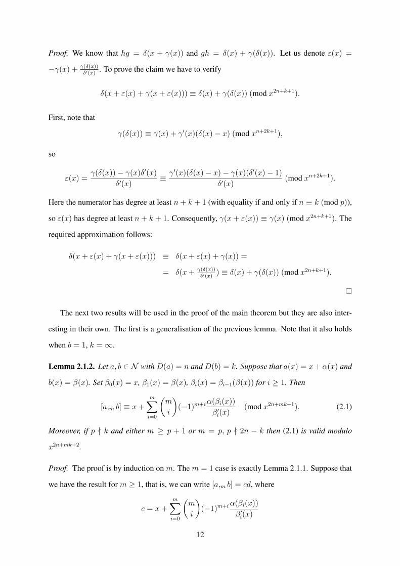
Proof. We know that hg = δ(x + γ(x)) and gh = δ(x) + γ(δ(x)). Let us denote ε(x) =
−γ(x) + γ(δ(x))δ′(x)
. To prove the claim we have to verify
δ(x+ ε(x) + γ(x+ ε(x))) ≡ δ(x) + γ(δ(x)) (mod x2n+k+1).
First, note that
γ(δ(x)) ≡ γ(x) + γ′(x)(δ(x)− x) (mod xn+2k+1),
so
ε(x) =γ(δ(x))− γ(x)δ′(x)
δ′(x)≡ γ′(x)(δ(x)− x)− γ(x)(δ′(x)− 1)
δ′(x)(mod xn+2k+1).
Here the numerator has degree at least n+ k + 1 (with equality if and only if n ≡ k (mod p)),
so ε(x) has degree at least n+ k + 1. Consequently, γ(x+ ε(x)) ≡ γ(x) (mod x2n+k+1). The
required approximation follows:
δ(x+ ε(x) + γ(x+ ε(x))) ≡ δ(x+ ε(x) + γ(x)) =
= δ(x+ γ(δ(x))δ′(x)
) ≡ δ(x) + γ(δ(x)) (mod x2n+k+1).
The next two results will be used in the proof of the main theorem but they are also inter-
esting in their own. The first is a generalisation of the previous lemma. Note that it also holds
when b = 1, k =∞.
Lemma 2.1.2. Let a, b ∈ N with D(a) = n and D(b) = k. Suppose that a(x) = x+α(x) and
b(x) = β(x). Set β0(x) = x, β1(x) = β(x), βi(x) = βi−1(β(x)) for i ≥ 1. Then
[a,m b] ≡ x+m∑i=0
(m
i
)(−1)m+iα(βi(x))
β′i(x)(mod x2n+mk+1). (2.1)
Moreover, if p - k and either m ≥ p + 1 or m = p, p - 2n − k then (2.1) is valid modulo
x2n+mk+2.
Proof. The proof is by induction on m. The m = 1 case is exactly Lemma 2.1.1. Suppose that
we have the result for m ≥ 1, that is, we can write [a,m b] = cd, where
c = x+m∑i=0
(m
i
)(−1)m+iα(βi(x))
β′i(x)
12
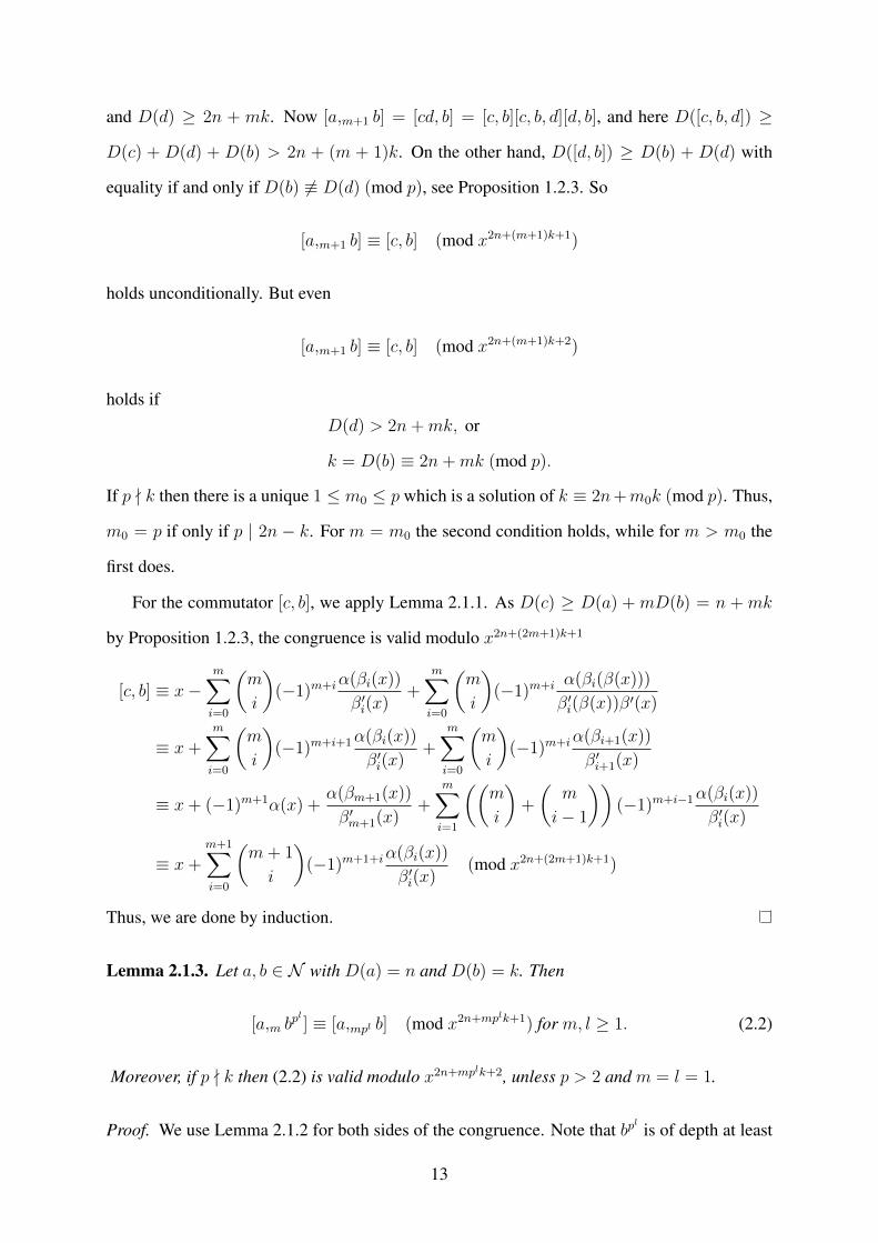
and D(d) ≥ 2n + mk. Now [a,m+1 b] = [cd, b] = [c, b][c, b, d][d, b], and here D([c, b, d]) ≥
D(c) + D(d) + D(b) > 2n + (m + 1)k. On the other hand, D([d, b]) ≥ D(b) + D(d) with
equality if and only if D(b) 6≡ D(d) (mod p), see Proposition 1.2.3. So
[a,m+1 b] ≡ [c, b] (mod x2n+(m+1)k+1)
holds unconditionally. But even
[a,m+1 b] ≡ [c, b] (mod x2n+(m+1)k+2)
holds ifD(d) > 2n+mk, or
k = D(b) ≡ 2n+mk (mod p).
If p - k then there is a unique 1 ≤ m0 ≤ p which is a solution of k ≡ 2n+m0k (mod p). Thus,
m0 = p if only if p | 2n − k. For m = m0 the second condition holds, while for m > m0 the
first does.
For the commutator [c, b], we apply Lemma 2.1.1. As D(c) ≥ D(a) + mD(b) = n + mk
by Proposition 1.2.3, the congruence is valid modulo x2n+(2m+1)k+1
[c, b] ≡ x−m∑i=0
(m
i
)(−1)m+iα(βi(x))
β′i(x)+
m∑i=0
(m
i
)(−1)m+i α(βi(β(x)))
β′i(β(x))β′(x)
≡ x+m∑i=0
(m
i
)(−1)m+i+1α(βi(x))
β′i(x)+
m∑i=0
(m
i
)(−1)m+iα(βi+1(x))
β′i+1(x)
≡ x+ (−1)m+1α(x) +α(βm+1(x))
β′m+1(x)+
m∑i=1
((m
i
)+
(m
i− 1
))(−1)m+i−1α(βi(x))
β′i(x)
≡ x+m+1∑i=0
(m+ 1
i
)(−1)m+1+iα(βi(x))
β′i(x)(mod x2n+(2m+1)k+1)
Thus, we are done by induction.
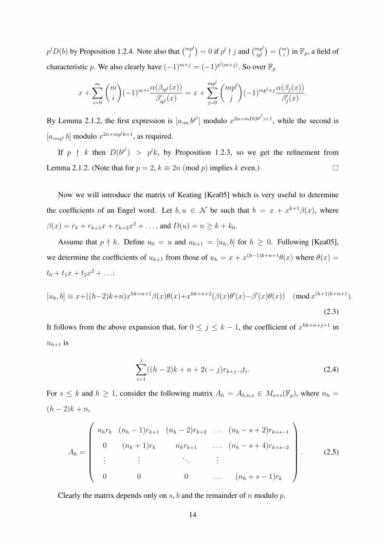
Lemma 2.1.3. Let a, b ∈ N with D(a) = n and D(b) = k. Then
[a,m bpl ] ≡ [a,mpl b] (mod x2n+mplk+1) for m, l ≥ 1. (2.2)
Moreover, if p - k then (2.2) is valid modulo x2n+mplk+2, unless p > 2 and m = l = 1.
Proof. We use Lemma 2.1.2 for both sides of the congruence. Note that bpl is of depth at least
13
plD(b) by Proposition 1.2.4. Note also that(mpl
j
)= 0 if pl - j and
(mpl
ipl
)=(mi
)in Fp, a field of
characteristic p. We also clearly have (−1)m+j = (−1)pl(m+j). So over Fp
x+m∑i=0
(m
i
)(−1)m+iα(βipl(x))
β′ipl
(x)= x+
mpl∑j=0
(mpl
j
)(−1)mp
l+jα(βj(x))
β′j(x).
By Lemma 2.1.2, the first expression is [a,m bpl ] modulo x2n+mD(bp
l)+1, while the second is
[a,mpl b] modulo x2n+mplk+1, as required.
If p - k then D(bpl) > plk, by Proposition 1.2.3, so we get the refinement from
Lemma 2.1.2. (Note that for p = 2, k ≡ 2n (mod p) implies k even.)
Now we will introduce the matrix of Keating [Kea05] which is very useful to determine
the coefficients of an Engel word. Let b, u ∈ N be such that b = x + xk+1β(x), where
β(x) = rk + rk+1x+ rk+2x2 + . . . , and D(u) = n ≥ k + k0.
Assume that p - k. Define u0 = u and uh+1 = [uh, b] for h ≥ 0. Following [Kea05],
we determine the coefficients of uh+1 from those of uh = x + x(h−1)k+n+1θ(x) where θ(x) =
t0 + t1x+ t2x2 + . . .:
[uh, b] ≡ x+((h−2)k+n)xhk+n+1β(x)θ(x)+xhk+n+2(β(x)θ′(x)−β′(x)θ(x)) (mod x(h+1)k+n+1).
(2.3)
It follows from the above expansion that, for 0 ≤ j ≤ k − 1, the coefficient of xhk+n+j+1 in
uh+1 is
j∑i=1
((h− 2)k + n+ 2i− j)rk+j−iti. (2.4)
For s ≤ k and h ≥ 1, consider the following matrix Ah = Ah,n,s ∈ Ms×s(Fp), where nh =
(h− 2)k + n,
Ah =
nhrk (nh − 1)rk+1 (nh − 2)rk+2 . . . (nh − s+ 2)rk+s−1
0 (nh + 1)rk nhrk+1 . . . (nh − s+ 4)rk+s−2
...... . . . ...
0 0 0 . . . (nh + s− 1)rk
. (2.5)
Clearly the matrix depends only on s, b and the remainder of n modulo p.
14
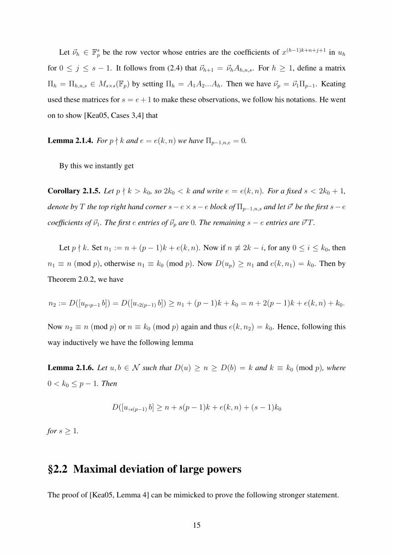
Let ~νh ∈ Fsp be the row vector whose entries are the coefficients of x(h−1)k+n+j+1 in uh
for 0 ≤ j ≤ s − 1. It follows from (2.4) that ~νh+1 = ~νhAh,n,s. For h ≥ 1, define a matrix
Πh = Πh,n,s ∈ Ms×s(Fp) by setting Πh = A1A2...Ah. Then we have ~νp = ~ν1Πp−1. Keating
used these matrices for s = e+ 1 to make these observations, we follow his notations. He went
on to show [Kea05, Cases 3,4] that
Lemma 2.1.4. For p - k and e = e(k, n) we have Πp−1,n,e = 0.
By this we instantly get
Corollary 2.1.5. Let p - k > k0, so 2k0 < k and write e = e(k, n). For a fixed s < 2k0 + 1,
denote by T the top right hand corner s− e× s− e block of Πp−1,n,s and let ~ν ′ be the first s− e
coefficients of ~ν1. The first e entries of ~νp are 0. The remaining s− e entries are ~ν ′T .
Let p - k. Set n1 := n + (p− 1)k + e(k, n). Now if n 6≡ 2k − i, for any 0 ≤ i ≤ k0, then
n1 ≡ n (mod p), otherwise n1 ≡ k0 (mod p). Now D(up) ≥ n1 and e(k, n1) = k0. Then by
Theorem 2.0.2, we have
n2 := D([up,p−1 b]) = D([u,2(p−1) b]) ≥ n1 + (p− 1)k + k0 = n+ 2(p− 1)k + e(k, n) + k0.
Now n2 ≡ n (mod p) or n ≡ k0 (mod p) again and thus e(k, n2) = k0. Hence, following this
way inductively we have the following lemma
Lemma 2.1.6. Let u, b ∈ N such that D(u) ≥ n ≥ D(b) = k and k ≡ k0 (mod p), where
0 < k0 ≤ p− 1. Then
D([u,s(p−1) b] ≥ n+ s(p− 1)k + e(k, n) + (s− 1)k0
for s ≥ 1.
§2.2 Maximal deviation of large powers
The proof of [Kea05, Lemma 4] can be mimicked to prove the following stronger statement.
15
Lemma 2.2.1. Suppose that n′ > n ≥ k are such that Theorem 2.0.2 holds for (k, n), and
Theorem 2.0.3 holds for (k, n′). If
n+ e(k, n) = n′ + e(k, n′)
then Theorem 2.0.3 also holds for (k, n).
By the definition of e(k, n) the sum n + e(k, n) is constant in the intervals k + pt ≤ n ≤
k + tp + k0. The lemma allows us to assume that k + k0 + tp ≤ n < k + (t + 1)p. If
n = k + k0 + pt then e(k, n) = 0, otherwise, e(k, n) = k0. We are going to assume this in the
proof of Theorem 2.0.3, below.
Let p - k and k + k0 + pt ≤ n ≤ k + (t+ 1)p for some nonnegative integer t. We define
e′(k, n) =
0 if k + k0 + pt < n < k + p(t+ 1),
k0 if n = k + k0 + pt or n = k + p(t+ 1).
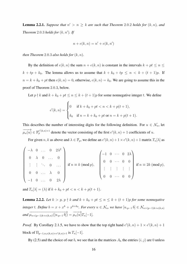
This describes the number of interesting digits for the following definition. For u ∈ Nn, let−−−→µn(u) ∈ Fe
′(k,n)+1p denote the vector consisting of the first e′(k, n) + 1 coefficients of u.
For given n, k as above and λ ∈ Fp, we define an e′(k, n) + 1× e′(k, n) + 1 matrix Tn[λ] as
−λ 0 . . . 0 2λ2
0 λ 0 . . . 0
...... . . . 0 . . .
0 0 . . . λ 0
−1 0 . . . 0 2λ
if n ≡ k (mod p),
−1 0 · · · 0 2λ
0 0 · · · 0 0
......
......
...
0 0 · · · 0 0
if n ≡ 2k (mod p),
and Tn[λ] = (λ) if k + k0 + pt < n < k + p(t+ 1).
Lemma 2.2.2. Let k > p, p - k and k + k0 + pt ≤ n ≤ k + (t + 1)p for some nonnegative
integer t. Define b = x + xk + xk+k0 . For every u ∈ Nn, we have [u,p−1 b] ∈ Nn+(p−1)k+e(k,n)
and−−−−−−−−−−−−−−−−−→µn+(p−1)k+e(k,n)([u,p−1 b]) =
−−−→µn(u)Tn[−1].
Proof. By Corollary 2.1.5, we have to show that the top right hand e′(k, n) + 1× e′(k, n) + 1
block of Πp−1,n,e(k,n)+e′(k,n)+1 is Tn[−1].
By (2.5) and the choice of our b, we see that in the matrices Ah the entries (i, j) are 0 unless
16
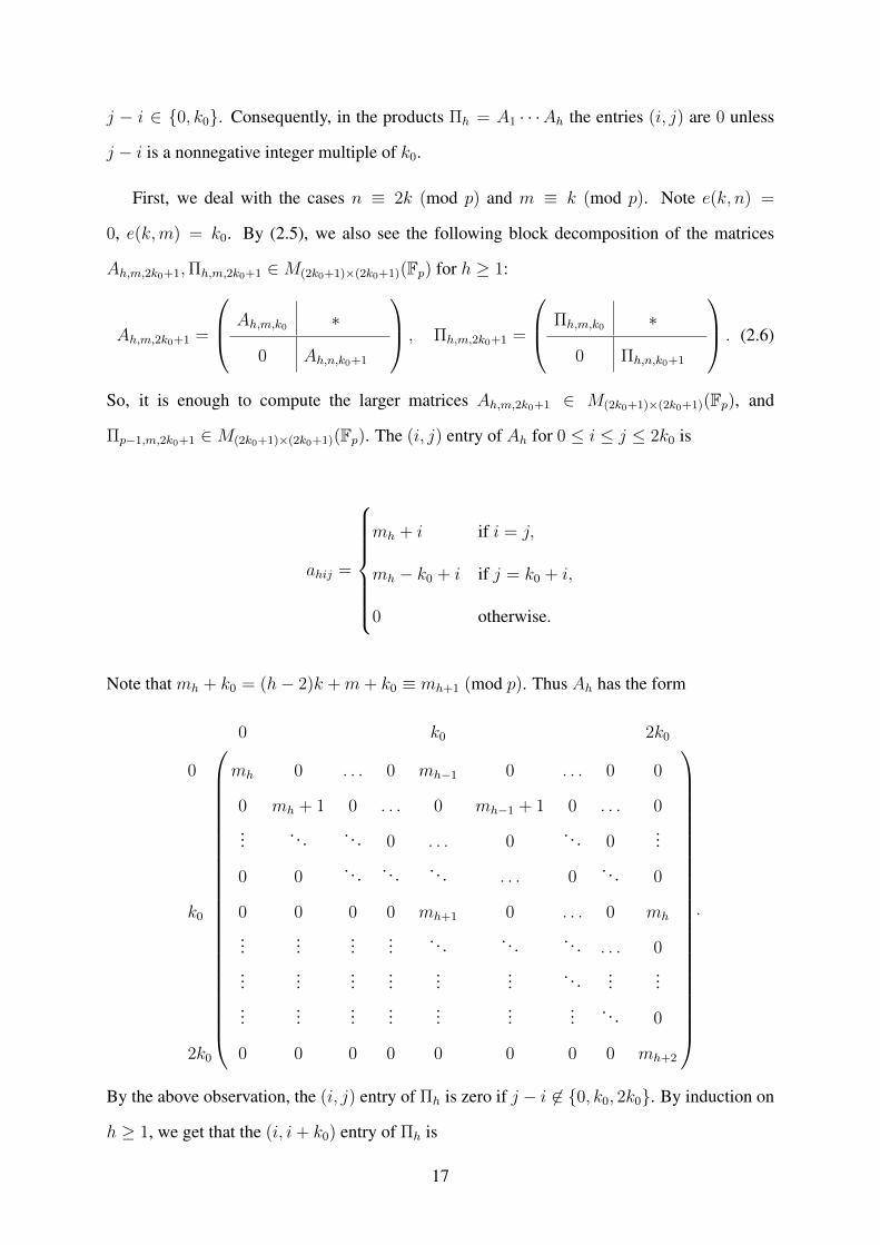
j − i ∈ {0, k0}. Consequently, in the products Πh = A1 · · ·Ah the entries (i, j) are 0 unless
j − i is a nonnegative integer multiple of k0.
First, we deal with the cases n ≡ 2k (mod p) and m ≡ k (mod p). Note e(k, n) =
0, e(k,m) = k0. By (2.5), we also see the following block decomposition of the matrices
Ah,m,2k0+1,Πh,m,2k0+1 ∈M(2k0+1)×(2k0+1)(Fp) for h ≥ 1:
Ah,m,2k0+1 =
Ah,m,k0 ∗
0 Ah,n,k0+1
, Πh,m,2k0+1 =
Πh,m,k0 ∗
0 Πh,n,k0+1
. (2.6)
So, it is enough to compute the larger matrices Ah,m,2k0+1 ∈ M(2k0+1)×(2k0+1)(Fp), and
Πp−1,m,2k0+1 ∈M(2k0+1)×(2k0+1)(Fp). The (i, j) entry of Ah for 0 ≤ i ≤ j ≤ 2k0 is
ahij =
mh + i if i = j,
mh − k0 + i if j = k0 + i,
0 otherwise.
Note that mh + k0 = (h− 2)k +m+ k0 ≡ mh+1 (mod p). Thus Ah has the form
0 k0 2k0
0 mh 0 . . . 0 mh−1 0 . . . 0 0
0 mh + 1 0 . . . 0 mh−1 + 1 0 . . . 0
... . . . . . . 0 . . . 0. . . 0
...
0 0. . . . . . . . . . . . 0
. . . 0
k0 0 0 0 0 mh+1 0 . . . 0 mh
......
...... . . . . . . . . . . . . 0
......
......
...... . . . ...
......
......
......
...... . . . 0
2k0 0 0 0 0 0 0 0 0 mh+2
.
By the above observation, the (i, j) entry of Πh is zero if j − i 6∈ {0, k0, 2k0}. By induction on
h ≥ 1, we get that the (i, i+ k0) entry of Πh is
17
(h−1∑t=1
(m1 + i)(m2 + i)...(mt + i)2(mt+3 + i)(mt+4 + i)...(mh+1 + i)
)
+(m0 + i)(m3 + i)...(mh+1 + i).
(2.7)
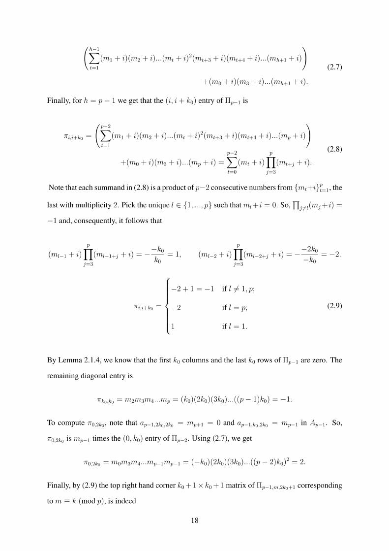
Finally, for h = p− 1 we get that the (i, i+ k0) entry of Πp−1 is
πi,i+k0 =
(p−2∑t=1
(m1 + i)(m2 + i)...(mt + i)2(mt+3 + i)(mt+4 + i)...(mp + i)
)
+(m0 + i)(m3 + i)...(mp + i) =
p−2∑t=0
(mt + i)
p∏j=3
(mt+j + i).
(2.8)
Note that each summand in (2.8) is a product of p−2 consecutive numbers from {mt+i}pt=1, the
last with multiplicity 2. Pick the unique l ∈ {1, ..., p} such thatml+i = 0. So,∏
j 6=l(mj+i) =
−1 and, consequently, it follows that
(ml−1 + i)
p∏j=3
(ml−1+j + i) = −−k0
k0
= 1, (ml−2 + i)
p∏j=3
(ml−2+j + i) = −−2k0
−k0
= −2.
πi,i+k0 =
−2 + 1 = −1 if l 6= 1, p;
−2 if l = p;
1 if l = 1.
(2.9)
By Lemma 2.1.4, we know that the first k0 columns and the last k0 rows of Πp−1 are zero. The
remaining diagonal entry is
πk0,k0 = m2m3m4...mp = (k0)(2k0)(3k0)...((p− 1)k0) = −1.
To compute π0,2k0 , note that ap−1,2k0,2k0 = mp+1 = 0 and ap−1,k0,2k0 = mp−1 in Ap−1. So,
π0,2k0 is mp−1 times the (0, k0) entry of Πp−2. Using (2.7), we get
π0,2k0 = m0m3m4...mp−1mp−1 = (−k0)(2k0)(3k0)...((p− 2)k0)2 = 2.
Finally, by (2.9) the top right hand corner k0 + 1×k0 + 1 matrix of Πp−1,m,2k0+1 corresponding
to m ≡ k (mod p), is indeed
18
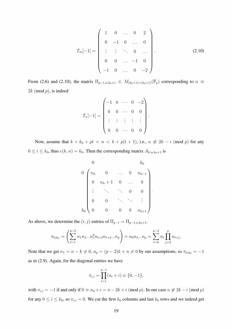
Tm[−1] =
1 0 . . . 0 2
0 −1 0 . . . 0
...... . . . 0 . . .
0 0 . . . −1 0
−1 0 . . . 0 −2
. (2.10)
From (2.6) and (2.10), the matrix Πp−1,n,k0+1 ∈ M(k0+1)×(k0+1)(Fp) corresponding to n ≡
2k (mod p), is indeed
Tn[−1] =
−1 0 · · · 0 −2
0 0 · · · 0 0
......
......
...
0 0 · · · 0 0
.
Now, assume that k + k0 + pt < n < k + p(t + 1), i.e., n 6≡ 2k − i (mod p) for any
0 ≤ i ≤ k0, thus e(k, n) = k0. Then the corresponding matrix Ah,n,k0+1 is
0 k0
0 nh 0 . . . 0 nh−1
0 nh + 1 0 . . . 0
... . . . . . . 0 0
0 0. . . . . . ...
k0 0 0 0 0 nh+1
.
As above, we determine the (i, j) entries of Πp−1 = Πp−1,n,k0+1.
π0,k0 =
(p−2∑t=1
n1n2...n2tnt+3nt+4...np
)+ n0n3...np =
p−2∑t=0
nt
p∏j=3
nt+j.
Note that we get n1 = n− k 6= 0, np = (p− 2)k + n 6= 0 by our assumptions, so π0,k0 = −1
as in (2.9). Again, for the diagonal entries we have
πi,i =
p−1∏t=1
(nt + i) ∈ {0,−1},
with πi,i = −1 if and only if 0 ≡ n0 + i = n− 2k+ i (mod p). In our case n 6≡ 2k− i (mod p)
for any 0 ≤ i ≤ k0, so πi,i = 0. We cut the first k0 columns and last k0 rows and we indeed get
19
the matrix
Tn[−1] = (−1).
Lemma 2.2.3. Let p > 2. Suppose k = k0 < p and k + k0 + pt ≤ n ≤ k + (t + 1)p for
some nonnegative integer t. If k < p− 1 then let b = x+ xk+1, otherwise, let b = x+ xk+1 +
x2k+1. For every u ∈ Nn we have [u,p−1 b] ∈ Nn+(p−1)k+e(k,n) and−−−−−−−−−−−−−−−−−→µn+(p−1)k+e(k,n)([u,p−1 b]) =
−−−→µn(u)Tn[λ], where λ = k−1
2if k = p− 1 and λ = k+1
2otherwise.
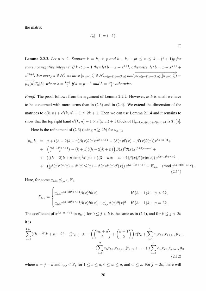
Proof. The proof follows from the argument of Lemma 2.2.2. However, as k is small we have
to be concerned with more terms than in (2.3) and in (2.4). We extend the dimension of the
matrices to e(k, n) + e′(k, n) + 1 ≤ 2k + 1. Then we can use Lemma 2.1.4 and it remains to
show that the top right hand e′(k, n) + 1× e′(k, n) + 1 block of Πp−1,n,e(k,n)+e′(k,n)+1 is Tn[λ].
Here is the refinement of (2.3) (using n ≥ 2k) for uh+1,
[uh, b] ≡ x+ ((h− 2)k + n)β(x)θ(x)xhk+n+1 + (β(x)θ′(x)− β′(x)θ(x))xhk+n+2+
+((
(h−1)k+n+12
)− (k + 1)((h− 2)k + n)
)β(x)2θ(x)x(h+1)k+n+1+
+ (((h− 2)k + n)β(x)2θ′(x) + ((3− h)k − n+ 1)β(x)β′(x)θ(x))x(h+1)k+n+2+
+(
12β(x)2θ′′(x) + β′(x)2θ(x)− β(x)β′(x)θ′(x)
)x(h+1)k+n+3 + Eh,n (mod x(h+2)k+n+2).
(2.11)
Here, for some qh,n, q′h,n ∈ Fp,
Eh,n =
qh,nx
(h+2)k+n+1β(x)3θ(x) if (h− 1)k + n > 2k,
qh,nx(h+2)k+n+1β(x)3θ(x) + q′h,nβ(x)θ(x)2 if (h− 1)k + n = 2k.
The coefficient of xhk+n+j+1 in uh+1 for 0 ≤ j < k is the same as in (2.4), and for k ≤ j < 2k
it is
k+a∑i=1
((h− 2)k + n+ 2i− j)rk+j−iti +
((nh + a
2
)+
(k + 1
2
))r2kta +
1∑i=0
c1irk+irk+1−i)ta−1
+(2∑i=0
c2irk+irk+2−i)ta−2 + · · ·+ (a∑i=0
cairk+irk+a−i)t0
(2.12)
where a = j − k and csw ∈ Fp for 1 ≤ s ≤ a, 0 ≤ w ≤ a, and w ≤ s. For j = 2k, there will
20
be an extra term in the coefficient of t0 and the rest will satisfy the above formula. But its value
is irrelevant for our proof.
We get again that the (i, j) entry of Πh is 0 unless j − i ∈ {0, k, 2k} as in Lemma 2.2.2.
Again, we assume first that n ≡ 2k (mod p) and m ≡ k (mod p) and hence e(k, n) =
0, e(k,m) = k. As a subcase, assume that k < p − 1 so b = x + xk+1. Now from (2.12) we
compute the entries of the matrix Ah,m,2k+1
ahij =
mh + i if i = j,(mh+i
2
)+(k+1
2
)if j = i+ k,
Ch,m if (i, j) = (0, 2k),
0 otherwise.
The value of Ch,m ∈ Fp is going to be irrelevant. By induction on h ≥ 1, we get that the
(i, i+ k) entry of Πh is(h∑t=1
(m1 + i)(m2 + i) · · · (mt + i)(mt+2 + i)(mt+3 + i) · · · (mh+1 + i)mt + i− 1
2
)
+
(k + 1
2
) h+1∑t=2
(m1 + i)(m2 + i) · · · (mt−2 + i)(mt+1 + i) · · · (mh+1 + i)
(2.13)
Consider h = p− 1. For i = 0, the first sum is 0, because m1 = 0 is a factor in each product.
For i > 0, pick the unique l ∈ {2, . . . , p} such that ml + i = 0 and observe that the first sum
has a single nonzero term, that for t = l − 1. Its value is k+12
. For i = 0, k, the second sum has
a single nonzero summand, two otherwise. For i = 0 the value is −k−12
, for i = k it is k+12
and
for i 6= 0, k the two terms add up to 0. So, finally
πi,i+k =
−k−12, if i=0;
k + 1, if i=k;
k+12, otherwise.
(2.14)
Note that Πp−2 has (0, 0) entry 0 and (0, k) entry k+12k
and Ap−1 has (k, 2k) entry k(k + 1) and
21

(2k, 2k) entry 0. So, π0,2k = (k+1)2
2. For the diagonal entries we again have
πi,i =
p−1∏h=1
(mh + i) ∈ {0,−1},
with πi,i = −1 if and only if 0 ≡ m0 + i = m− 2k + i ≡ −k + i (mod p). Put λ = k+126= 0
as k < p− 1. Now we have the claimed matrix
Tm[λ] =
−λ 0 . . . 0 2λ2
0 λ 0 . . . 0
...... . . . 0 . . .
0 0 . . . λ 0
−1 0 . . . 0 2λ
.
As (2.6) is still valid, we also have
Tn[λ] =
−1 0 · · · 0 2λ
0 0 · · · 0 0
......
......
...
0 0 · · · 0 0
.
Now suppose that k = p − 1 so take b = x + xp + x2p−1. We continue to assume that
n ≡ 2k (mod p) and m ≡ k (mod p), hence e(k, n) = 0, e(k,m) = k. By using (2.11), (2.12),
we have the corresponding matrix Ah,m,2k+1 whose (i, j) entries for 0 ≤ i, j ≤ 2k are
ahij =
mh + i if i = j,
mh + i− k +(mh+i
2
)+(k+1
2
)if j = k + i,
Dh,m if (i, j) = (0, 2k)
0 otherwise.
The value of Dh,m ∈ Fp is uninteresting, as before. Again the (i, j) entry of Πh,m,2k+1 is zero
if j − i 6∈ {0, k, 2k}. By the value of ah,i,i+k, we get that (i, i + k) entry of Πh is the sum of
22
(2.13) and (2.7). Therefore,
πi,i+k =
−k−12
+ 1 = −k−12, if i = 0;
k + 1− 2 = k − 1, if i = k;
k+12− 1 = k−1
2, otherwise.
Note that Πp−2 has (0, 0) entry 0 and (0, k) entry k+12k
+ −1k
= k−12k
. On the other hand, Ap−1
has (k, 2k) entry −2k + k(k + 1) = k(k − 1) and (2k, 2k) entry 0. Thus, π0,2k = (k−1)2
2. For
the diagonal entries, we again have
πi,i =
p−1∏h=1
(mh + i) ∈ {0,−1},
with πi,i = −1 if and only if 0 ≡ m0 + i = m− 2k + i ≡ −k + i (mod p). Put λ = k−12
. (We
use the assumption p > 2 to claim λ 6= 0). We obtained the claimed matrix
Tm[λ] =
−λ 0 . . . 0 2λ2
0 λ 0 . . . 0
...... . . . 0 . . .
0 0 . . . λ 0
−1 0 . . . 0 2λ
.
We get Tn[λ] in a similar way exactly as above.
Assume finally that k + k0 + pt < n < k + p(t + 1), that is, n 6≡ 2k − i (mod p) for any
0 ≤ i ≤ k0, then e(k, n) = k0. Of course k < p− 1. So we take the element b = x+ xk+1 and
obtain the corresponding matrix Tn[λ] = (k+12
) (from (2.14)) exactly as in Lemma 2.2.2.
Proof of Theorem 2.0.3. Suppose that p - k. By the remark before Lemma 2.2.1 we may as-
sume that k + k0 + pt ≤ n < k + (t + 1)p, for some integer t ≥ 0. If n = k + k0 + pt then
e(k, n) = 0, otherwise, e(k, n) = k0.
Let g−1 = x+ xk+1 + xk+k0+1, or x+ xk+1 as in Lemma 2.2.2 and Lemma 2.2.3. We pick
u = u0 ∈ Nn, but its leading coefficient, α, will be chosen appropriately later. Set f−1 = g−1u
and then um = gpmf−p
m . Let nm = n+ (pm − 1)k + pm−pp−1
k0 + e(k, n).
We prove that D(um) = nm by induction on m. We assume m ≥ 1 and that for every
23
smaller index the theorem holds. Note that nm = nm−1 + (p− 1)pm−1k + pm−1k0.
By [LGM02, Proposition 1.1.32(i)], we have
um ≡ upm−1[um−1, g−pm−1
](p2)[um−1,2 g
−pm−1
](p3) . . . [um−1,p−1 g
−pm−1
] mod K(g−pm−1
, um−1)
where K(g−pm−1
, um−1) is the normal closure in N of the set of all formal basic commutators
in {g−pm−1, um−1} of weight at least p and of weight at least 2 in um−1 and also the p-th
powers of all basic commutators of weight at least 3 and of weight at least 2 in um−1. The only
weight p commutator with weight 2 in um−1 is w = [[um−1,p−2 g−pm−1
], um−1]. We denote its
multiplicity by δ0. (The exact value δ0 = p2 − p− 1 is irrelevant for our proof.)
If m = 1 and nm−1 = n = k + k0 then e(k, n) = 0 and e′(k, n) = k0 so D([u,p−1 g−1]) =
n + (p − 1)k = n + (p − 1)k + e(k, n). The element w in K(g−1, u) has depth exactly
2n+ (p− 2)k = n+ (p− 1)k+ e(k, n) + e′(k, n), every other element in K(g−1, u) has larger
depth. The leading coefficient of w is
(n− k)αn(n+ k) · · · (n+ (p− 4)k)α(p− 2)k = −2α2,
where α is the leading coefficient of u. If nm−1 > k + k0 then every element in K(g−pm−1
, u)
has depth at least 2nm−1 + (p− 2)k > nm−1 + (p− 1)k + e(k, nm−1) + e′(k, nm−1).
Also note that D([um−1,i g−pm−1
](pi+1)) ≥ p(nm−1 + k) > nm−1 + (p− 1)k+ e(k, nm−1) +
e′(k, nm−1) for 1 ≤ i ≤ p − 2 for every nm−1 ≥ k + k0. Let nm−1 be the remainder of nm−1
modulo p. Then D(upm−1) ≥ pnm−1 + nm−1 = nm−1 + (p − 1)k + k0 + (p − 2)k0 + (p −
1)(nm−1 − k − k0) + nm−1 > nm−1 + (p− 1)k + e(k, nm−1) + e′(k, nm−1).
We conclude that
−−−−−→µnm(um) =
−−−−−−−−−−−−−−−−→µnm([um−1,p−1 g
−pm−1]) if nm−1 > k + k0,
−−−−−−−−−−→µn1([u,p−1 g
−1]) + (0, . . . , 0,−2δ0α2) if m = 1, n = k + k0.
(2.15)
Suppose that m > 1. By the last line of Lemma 2.1.3 (which holds in our case, as p−1 = 1
would imply p = 2),
[um−1,p−1 g−pm−1
] ≡ [um−1,(p−1)pm−1 g−1] (mod x2nm−1+(p−1)pm−1k+2).
24
Now
2nm−1 + (p− 1)pm−1k + 2 = nm + nm−1 − pm−1k0 + 2 =
nm + n+ (pm−1 − 1)k + (−pm−1 +pm−1 − pp− 1
)k0 + e(k, n) + 2 > nm + e′(k, nm) + 1.
So, we obtain−−−−−→µnm(um) =
−−−−−−−−−−−−−−−−−−→µnm([um−1,(p−1)pm−1 g−1]) for m > 1. By induction and by (2.15),
we have
−−−−−→µnm(um) =
−−−−−−−−−−−−−→µnm([u1,pm−p g
−1]) for m > 1,
−−−−−−−−−−−−→µnm([u,pm−1 g
−1]) for m ≥ 1 if n > k + k0.
(2.16)
After these preliminary observations we turn to the proof.
First, let k+k0 +pt < n < k+ (t+ 1)p. Then e′(k, n) = 0 and e(k, n) = k0. Lemma 2.2.2
or Lemma 2.2.3 shows that for any u ∈ Nn of depth n we have D([u,s(p−1) g−1]) = n+ s(p−
1)k + sk0 for every s ≥ 1. Thus, (2.16) implies that
D(um) = D([um−1,p−1 g−pm−1
]) = D([u,pm−1 g−1]) = nm,
as required.
Now suppose n = k + k0 + tp. Then e′(k, n) = k0, e(k, n) = 0. Recall that α 6= 0 denotes
the leading coefficient of u ∈ Nn. If k > p then λ = −1, if k = p − 1 then λ = k−12
and
if k < p − 1 then λ = k+12
. Then Lemma 2.2.2 or Lemma 2.2.3 shows that for the first k0
coefficients of v = [u,p−1 b] we have
−−−−→µn1(v) = (−α, 0, . . . , 0, 2λα),
where λ ∈ Fp nonzero. By (2.15),
−−−−−−−→µn1(g
pf−p) = (−α, . . . , 0, 2λα− 2δα2),
where δ = δ0 if n = k + k0 and δ = 0 otherwise. The leading coefficient is −α 6= 0,
so D(u1) = D(gpf−p) = n + (p − 1)k + e(k, n) = n1 holds. Now n1 ≡ k (mod p), so
e′(k, n1) = e(k, n1) = k0.
We apply Lemma 2.2.2 or Lemma 2.2.3 again to get
D(u2) = D([u1,p−1 g−p]) = D([u1,(p−1)p g
−1]) = n2.
25
We also obtain
−−−−−−−−→µn2(g
p2f−p2
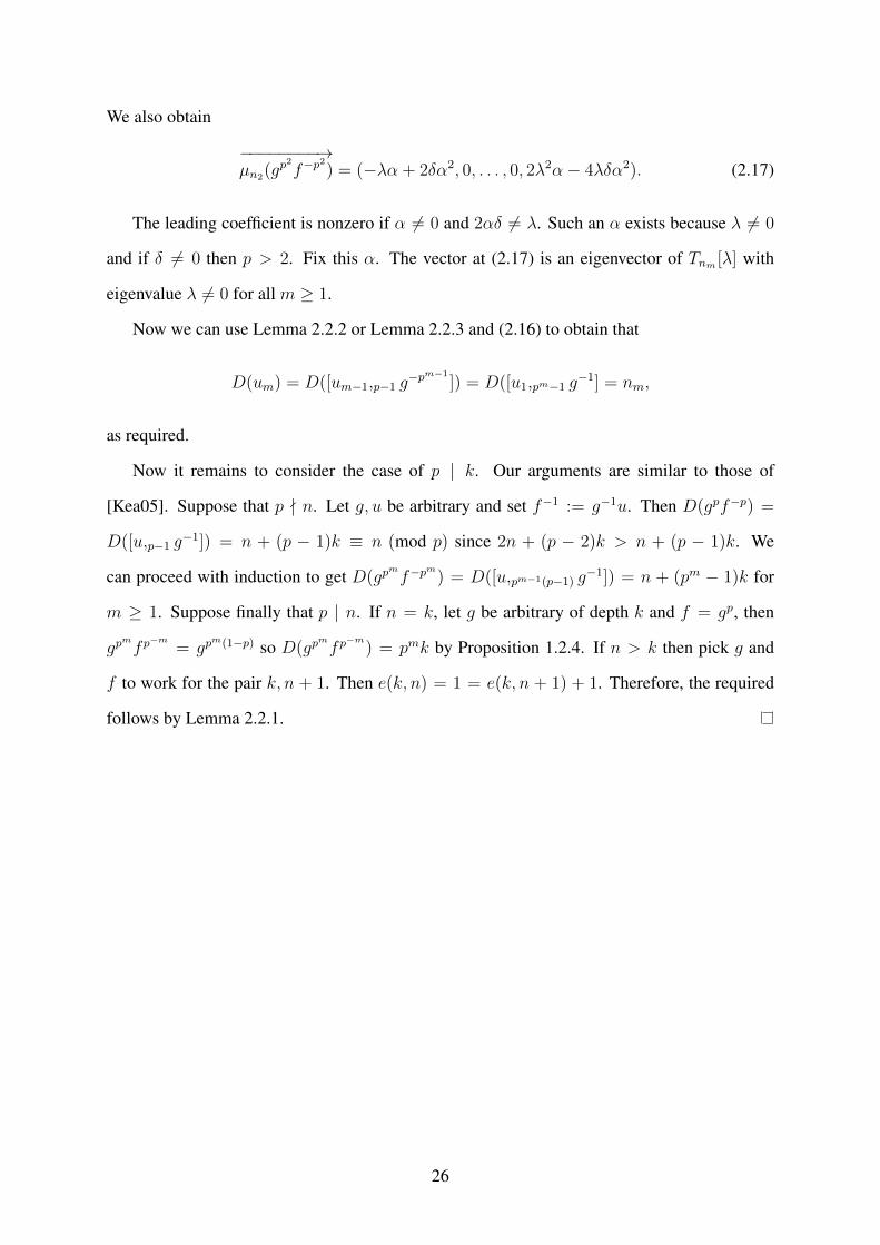
) = (−λα + 2δα2, 0, . . . , 0, 2λ2α− 4λδα2). (2.17)
The leading coefficient is nonzero if α 6= 0 and 2αδ 6= λ. Such an α exists because λ 6= 0
and if δ 6= 0 then p > 2. Fix this α. The vector at (2.17) is an eigenvector of Tnm [λ] with
eigenvalue λ 6= 0 for all m ≥ 1.
Now we can use Lemma 2.2.2 or Lemma 2.2.3 and (2.16) to obtain that
D(um) = D([um−1,p−1 g−pm−1
]) = D([u1,pm−1 g−1] = nm,
as required.
Now it remains to consider the case of p | k. Our arguments are similar to those of
[Kea05]. Suppose that p - n. Let g, u be arbitrary and set f−1 := g−1u. Then D(gpf−p) =
D([u,p−1 g−1]) = n + (p − 1)k ≡ n (mod p) since 2n + (p − 2)k > n + (p − 1)k. We
can proceed with induction to get D(gpmf−p
m) = D([u,pm−1(p−1) g
−1]) = n + (pm − 1)k for
m ≥ 1. Suppose finally that p | n. If n = k, let g be arbitrary of depth k and f = gp, then
gpmfp−m
= gpm(1−p) so D(gp
mfp−m
) = pmk by Proposition 1.2.4. If n > k then pick g and
f to work for the pair k, n + 1. Then e(k, n) = 1 = e(k, n + 1) + 1. Therefore, the required
follows by Lemma 2.2.1.
26
CHAPTER
3Characteristic 2
In the previous chapter we showed that the depth of gpmf−pm can be determined by finding the
depth of [u,s(p−1) g−1] where s = pm−1
p−1. This argument fails for p = 2 and k = 1. The main rea-
son behind it is that if D(g−1) = 1 then the sequence D(g−1), D(g−2), D(g−22), . . . increases
more rapidly. However, when p = 2 the 2m-th powers of an element can be computed more
easily than when p ≥ 3. Therefore, the matrix of Keating can be used to compute [u, g−2m ] for
m ≥ 1, and the problem can be reduced to determine D([u, g−1, g−2, g−22 , g−23 , . . . , g2m−1]).
It turns out that the bound is almost the double of Keating’s bound for p = 2, k = 1. Recall
that by Definition 2.0.1, e(1, n) = 1 if n is odd, otherwise, zero . Denote Dm := D(g2mf−2m),
our main result is the following
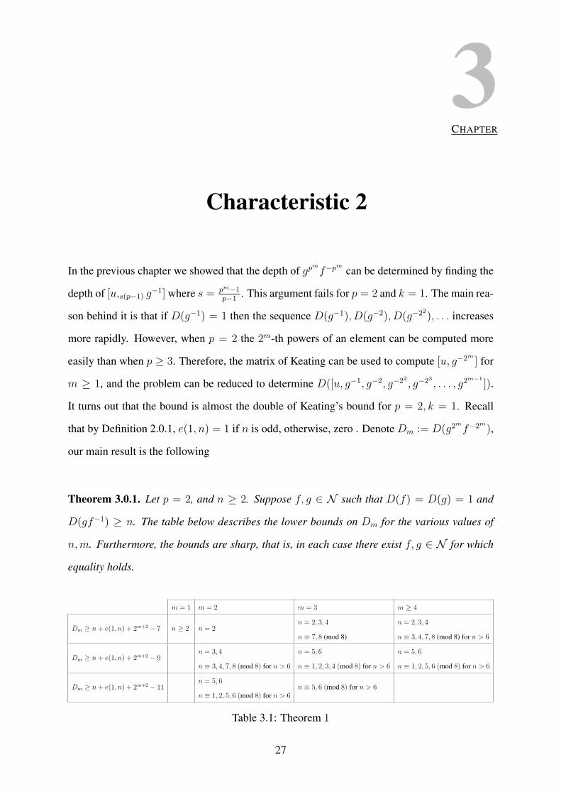
Theorem 3.0.1. Let p = 2, and n ≥ 2. Suppose f, g ∈ N such that D(f) = D(g) = 1 and
D(gf−1) ≥ n. The table below describes the lower bounds on Dm for the various values of
n,m. Furthermore, the bounds are sharp, that is, in each case there exist f, g ∈ N for which
equality holds.
m = 1 m = 2 m = 3 m ≥ 4
Dm ≥ n+ e(1, n) + 2m+2 − 7 n ≥ 2 n = 2n = 2, 3, 4
n ≡ 7, 8 (mod 8)
n = 2, 3, 4
n ≡ 3, 4, 7, 8 (mod 8) for n > 6
Dm ≥ n+ e(1, n) + 2m+2 − 9n = 3, 4
n ≡ 3, 4, 7, 8 (mod 8) for n > 6
n = 5, 6
n ≡ 1, 2, 3, 4 (mod 8) for n > 6
n = 5, 6
n ≡ 1, 2, 5, 6 (mod 8) for n > 6
Dm ≥ n+ e(1, n) + 2m+2 − 11n = 5, 6
n ≡ 1, 2, 5, 6 (mod 8) for n > 6n ≡ 5, 6 (mod 8) for n > 6
Table 3.1: Theorem 1
27
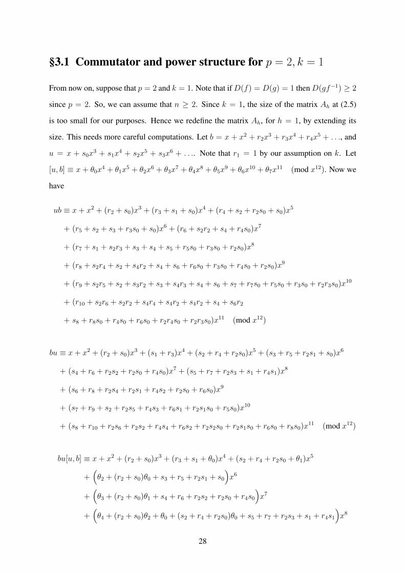
§3.1 Commutator and power structure for p = 2, k = 1
From now on, suppose that p = 2 and k = 1. Note that ifD(f) = D(g) = 1 thenD(gf−1) ≥ 2
since p = 2. So, we can assume that n ≥ 2. Since k = 1, the size of the matrix Ah at (2.5)
is too small for our purposes. Hence we redefine the matrix Ah, for h = 1, by extending its
size. This needs more careful computations. Let b = x + x2 + r2x3 + r3x
4 + r4x5 + . . ., and
u = x + s0x3 + s1x
4 + s2x5 + s3x
6 + . . .. Note that r1 = 1 by our assumption on k. Let
[u, b] ≡ x+ θ0x4 + θ1x
5 + θ2x6 + θ3x
7 + θ4x8 + θ5x
9 + θ6x10 + θ7x
11 (mod x12). Now we
have
ub ≡ x+ x2 + (r2 + s0)x3 + (r3 + s1 + s0)x4 + (r4 + s2 + r2s0 + s0)x5
+ (r5 + s2 + s3 + r3s0 + s0)x6 + (r6 + s2r2 + s4 + r4s0)x7
+ (r7 + s1 + s2r3 + s3 + s4 + s5 + r5s0 + r3s0 + r2s0)x8
+ (r8 + s2r4 + s2 + s4r2 + s4 + s6 + r6s0 + r3s0 + r4s0 + r2s0)x9
+ (r9 + s2r5 + s2 + s3r2 + s3 + s4r3 + s4 + s6 + s7 + r7s0 + r5s0 + r3s0 + r2r3s0)x10
+ (r10 + s2r6 + s2r2 + s4r4 + s4r2 + s4r2 + s4 + s6r2
+ s8 + r8s0 + r4s0 + r6s0 + r2r4s0 + r2r3s0)x11 (mod x12)
bu ≡ x+ x2 + (r2 + s0)x3 + (s1 + r3)x4 + (s2 + r4 + r2s0)x5 + (s3 + r5 + r2s1 + s0)x6
+ (s4 + r6 + r2s2 + r2s0 + r4s0)x7 + (s5 + r7 + r2s3 + s1 + r4s1)x8
+ (s6 + r8 + r2s4 + r2s1 + r4s2 + r2s0 + r6s0)x9
+ (s7 + r9 + s2 + r2s5 + r4s3 + r6s1 + r2s1s0 + r5s0)x10
+ (s8 + r10 + r2s6 + r2s2 + r4s4 + r6s2 + r2s2s0 + r2s1s0 + r6s0 + r8s0)x11 (mod x12)
bu[u, b] ≡ x+ x2 + (r2 + s0)x3 + (r3 + s1 + θ0)x4 + (s2 + r4 + r2s0 + θ1)x5
+(θ2 + (r2 + s0)θ0 + s3 + r5 + r2s1 + s0
)x6
+(θ3 + (r2 + s0)θ1 + s4 + r6 + r2s2 + r2s0 + r4s0
)x7
+(θ4 + (r2 + s0)θ2 + θ0 + (s2 + r4 + r2s0)θ0 + s5 + r7 + r2s3 + s1 + r4s1
)x8
28

+(θ5 + (r2 + s0)θ3 + (s2 + r4 + r2s0)θ1
+s6 + r8 + r2s4 + r2s1 + r4s2 + r2s0 + r6s0
)x9
+(θ6 + θ1 + (r2 + s0)θ4 + (s2 + r4 + r2s0)θ2 + (s4 + r6 + r2s2 + r2s0 + r4s0)θ0
+s7 + r9 + s2 + r2s5 + r4s3 + r6s1
)x10
+(θ7 + (r2 + s0)θ5 + (r2 + s0)θ1 + (s4 + r2s2 + r6 + r2s0 + r4s0)θ1
+(s2 + r4 + r2s0)θ3 + s8 + r10 + r2s6 + r2s2 + r4s4 + r6s2
+(r2s2 + r2s1 + r6 + r8)s0
)x11 (mod x12).
By solving the equation bu[u, b] ≡ ub (mod x12), we can get the commutator [u, b] mod
(mod x12) which is
[u, b] ≡ x+ s0x4 + s0x
5 +[(r2 + r3 + 1)s0 + r2s1 + s2
]x6 + s0x
7
+[(1 + r2(r3 + 1) + r2s1 + r4 + r5)s0 + (r2 + r4)s1 + (r2 + r3)s2 + (r2 + 1)s3 + s4
]x8
+[(r2 + r3 + s2)s0 + r2s1 + s2 + s4
]x9 +
[Bs0 + r6s1 + (r2(1 + r3) + r4 + r5 + 1)s2
+ (r4 + r2 + 1)s3 + (r2 + r3 + 1)s4 + r2s5 + s6
]x10
+[Cs0 + r2s1 + r2s2 + (r2 + 1)s4
]x11 (mod x12)
where B,C are polynomials in the coefficients of u, and b whose explicit expressions are
irrelevant. Let ~ν = (s0, s1, s2, . . . , s7) and ~ν1 = (θ0, θ1, θ2, . . . , θ7) be the coefficients vectors
of u, [u, b] for the terms x3+i and x4+i, respectively, for i ≥ 0. Then the formula above gives us
~νAb,2 = ~ν1, where Ab,2 is
1 1 r2 + r3 + 1 1 1 + r2(r3 + 1) + r2s1 + r4 + r5 r2 + r3 + s2 ∗ ∗
0 0 r2 0 r2 + r4 r2 r6 r2
0 0 1 0 r2 + r3 1 r2 + r2r3 + r4 + r5 + 1 r2
0 0 0 0 r2 + 1 0 r4 + r2 + 1 0
0 0 0 0 1 1 r2 + r3 + 1 r2 + 1
0 0 0 0 0 0 r2 0
0 0 0 0 0 0 1 0
0 0 0 0 0 0 0 0
.
(3.1)
29
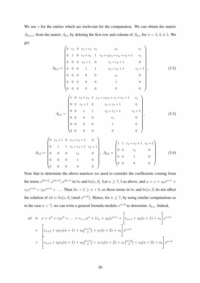
We use ∗ for the entries which are irrelevant for the computation. We can obtain the matrix
Ab,n+1 from the matrix Ab,n by deleting the first row and column of Ab,n for n = 2, 3, 4, 5. We
get
Ab,3 =
0 r2 0 r2 + r4 r2 r6 r2
0 1 0 r2 + r3 1 r2 + r2r3 + r4 + r5 + 1 r2
0 0 0 r2 + 1 0 r4 + r2 + 1 0
0 0 0 1 1 r2 + r3 + 1 r2 + 1
0 0 0 0 0 r2 0
0 0 0 0 0 1 0
0 0 0 0 0 0 0
, (3.2)
Ab,4 =
1 0 r2 + r3 1 r2 + r2r3 + r4 + r5 + 1 r2
0 0 r2 + 1 0 r4 + r2 + 1 0
0 0 1 1 r2 + r3 + 1 r2 + 1
0 0 0 0 r2 0
0 0 0 0 1 0
0 0 0 0 0 0
, (3.3)
Ab,5 =
0 r2 + 1 0 r4 + r2 + 1 0
0 1 1 r2 + r3 + 1 r2 + 1
0 0 0 r2 0
0 0 0 1 0
0 0 0 0 0
, Ab,6 =
1 1 r2 + r3 + 1 r2 + 1
0 0 r2 0
0 0 1 0
0 0 0 0
. (3.4)
Note that to determine the above matrices we need to consider the coefficients coming from
the terms x2n+2, x2n+3, x2n+4 in bu and bu[u, b]. Let n ≥ 7, b as above, and u = x + s0xn+1 +
s1xn+2 + s2x
n+3 + . . .. Then 2n + 2 ≥ n + 9, so those terms in bu and bu[u, b] do not affect
the solution of ub ≡ bu[u, b] (mod xn+9). Hence, for n ≥ 7, by using similar computations as
in the case n < 7, we can write a general formula modulo xn+9 to determine Ab,n. Indeed,
ub ≡ x+ x2 + r2x3 + . . .+ rn−1x
n + (rn + s0)xn+1 +
[rn+1 + s0(n+ 1) + s1
]xn+2
+
[rn+2 + s0r2(n+ 1) + s0
(n+1
2
)+ s1(n+ 2) + s2
]xn+3
+
[rn+3 + s0r3(n+ 1) + s0
(n+1
3
)+ s1r2(n+ 2) + s1
(n+2
2
)+ s2(n+ 3) + s3
]xn+4
30
+
[rn+4 + s0r4(n+ 1)s0r2
(n+1
2
)+ s0r2
(n+1
3
)+ s0
(n+1
4
)+ s1r3(n+ 2) + s1
(n+2
3
)+s2r2(n+ 3) + s2
(n+3
2
)+ s3(n+ 4) + s4
]xn+5
+
[rn+5 + s0r5(n+ 1) + s0r3
(n+1
2
)+ s0r2
(n+1
3
)+ s0
(n+1
5
)+ s1r4(n+ 2)
+s1r2
(n+2
2
)+ s1r2
(n+2
3
)+ s1
(n+2
4
)+ s2r3(n+ 3) + s2
(n+3
3
)+ s3r2(n+ 4)
+s3
(n+4
2
)+ s4(n+ 5) + s5
]xn+6
+
[rn+6 + s0r6(n+ 1) + s0r3
(n+1
2
)+ s0r4
(n+1
3
)+ s0r2
(n+1
3
)+ s0r2
(n+1
5
)+s0
(n+1
6
)+ s1r5(n+ 2) + s1r3
(n+2
3
)+ s1r2
(n+2
3
)+ s1
(n+2
5
)+ s2r4(n+ 3)
+s2r2
(n+3
2
)+ s2r2
(n+3
3
)+ s2
(n+3
4
)+ s3r3(n+ 4) + s3
(n+4
3
)+ s4r2(n+ 5)
+s4
(n+5
2
)+ s5(n+ 6) + s6
]xn+7
+
[rn+7 + s0r7(n+ 1) + s0r5
(n+1
3
)+ s0r3
(n+1
3
)+ s0r2r3
(n+1
3
)+ s0r3
(n+1
5
)+s0
(n+1
7
)+ s1r6(n+ 2) + s1r3
(n+2
2
)+ s1r4
(n+2
3
)+ s1r2
(n+2
3
)+ s1r2
(n+2
5
)+s1
(n+2
6
)+ s2r5(n+ 3) + s2r3
(n+3
3
)+ s2r2
(n+3
3
)+ s2
(n+3
5
)+ s3r4(n+ 4)
+s3r2
(n+4
2
)+ s3r2
(n+4
3
)+ s3
(n+4
4
)+ s4r3(n+ 5) + s4
(n+5
3
)+ s5r2(n+ 6)
+s5
(n+6
2
)+ s6(n+ 7) + s7
]xn+8 (mod xn+9),
bu ≡ x+ x2 + r2x3 + . . .+ rn−1x
n + (rn + s0)xn+1 + (rn+1 + s1)xn+2 + (r2s0 + s2)xn+3
+(r2s1 + s3)xn+4 + (r2s2 + r4s0 + s4)xn+5 + (r2s3 + r4s1 + s5)xn+6
+(r2s4 + r4s2 + r6s0 + s6)xn+7 + (r2s5 + r4s3 + r6s1 + s7)xn+8 (mod xn+9).
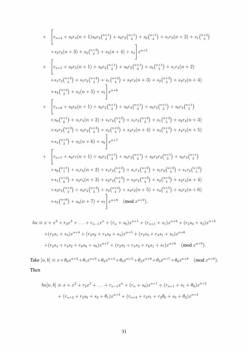
Take [u, b] ≡ x+θ0xn+2+θ1x
n+3+θ2xn+4+θ3x
n+5+θ4xn+6+θ5x
n+7+θ6xn+8 (mod xn+9).
Then
bu[u, b] ≡ x+ x2 + r2x3 + . . .+ rn−1x
n + (rn + s0)xn+1 + (rn+1 + s1 + θ0)xn+2
+ (rn+2 + r2s0 + s2 + θ1)xn+3 + (rn+3 + r2s1 + r2θ0 + s3 + θ2)xn+4
31

+ (rn+4 + r2s2 + r4s0 + r2θ1 + s4 + θ3)xn+5
+ (rn+5 + r2s3 + r4s1 + r2θ2 + r4θ0 + s5 + θ4)xn+6
+ (rn+6 + r2s4 + r4s2 + r6s0 + r4θ1 + r2θ3 + s6 + θ5)xn+7
+ (rn+7 + r2s5 + r4s3 + r6s1 + r6θ0 + r4θ2 + r2θ4 + s7 + θ6)xn+8 (mod xn+9).
Now we have
[u, b] ≡ x+
[(n+ 1)s0
]xn+2 +
[(nr2 +
(n+1
2
))s0 + ns1
]xn+3
+
[(n+ 1)(r2 + r3) +
(n+1
3
))s0 +
((n+ 1)r2 +
(n+2
2
))s1 + (n+ 1)s2
]xn+4
+
[(n(r2 + r4) +
(n+1
3
)r2 +
(n+1
4
))s0 +
(n(r2 + r3) +
(n+2
3
))s1
+(nr2 +
(n+3
2
))+ ns3
]xn+5
+
[((n+ 1)(r2 + r2r3 + r4 + r5) +
(n+1
3
)r3 +
(n+1
5
))s0
+(
(n+ 1)(r2 + r4) +(n+2
3
)r2 +
(n+2
4
))s1 +
((n+ 1)(r2 + r3) +
(n+3
3
))s2
+(
(n+ 1)r2 +(n+4
2
))s3 + (n+ 1)s4
]xn+6
+
[(n(r2 + r6) +
(n+1
4
)r2 +
(n+1
2
)(r4 + r3) +
(n+1
3
)r4 +
(n+1
5
)r2 +
(n+1
6
))s0
+(n(r2 + r2r3 + r4 + r5) +
(n+2
3
)r3 +
(n+2
5
))s1
+(n(r2 + r4) +
(n+3
3
)r2 +
(n+3
4
))s2 +
(n(r2 + r3) +
(n+4
3
))s3
+(nr2 +
(n+5
2
))s4 + ns5
]xn+7
+
[((n+ 1)(r6 + r3r4 + r2(1 + r3 + r5) + r7)
+(n+1
3
)(r3 + r4 + r5) +
(n+1
5
)(r2 + r3) +
(n+1
7
))s0 +
((n+ 1)(r2 + r6)
+(n+2
2
)(r3 + r4) +
(n+2
3
)r4 +
(n+2
4
)r2 +
(n+2
5
)r2 +
(n+2
6
))s1
+(
(n+ 1)(r2 + r4 + r5 + r2r3) +(n+3
3
)r3 +
(n+3
5
))s2
+(
(n+ 1)(r4 + r2) +(n+4
3
)r2 +
(n+4
4
))s3 +
((n+ 1)(r2 + r3) +
(n+5
3
))s4
+(
(n+ 1)r2 +(n+6
2
))s5 +
((n+ 1)
)s6
]xn+8 (mod xn+9).
32
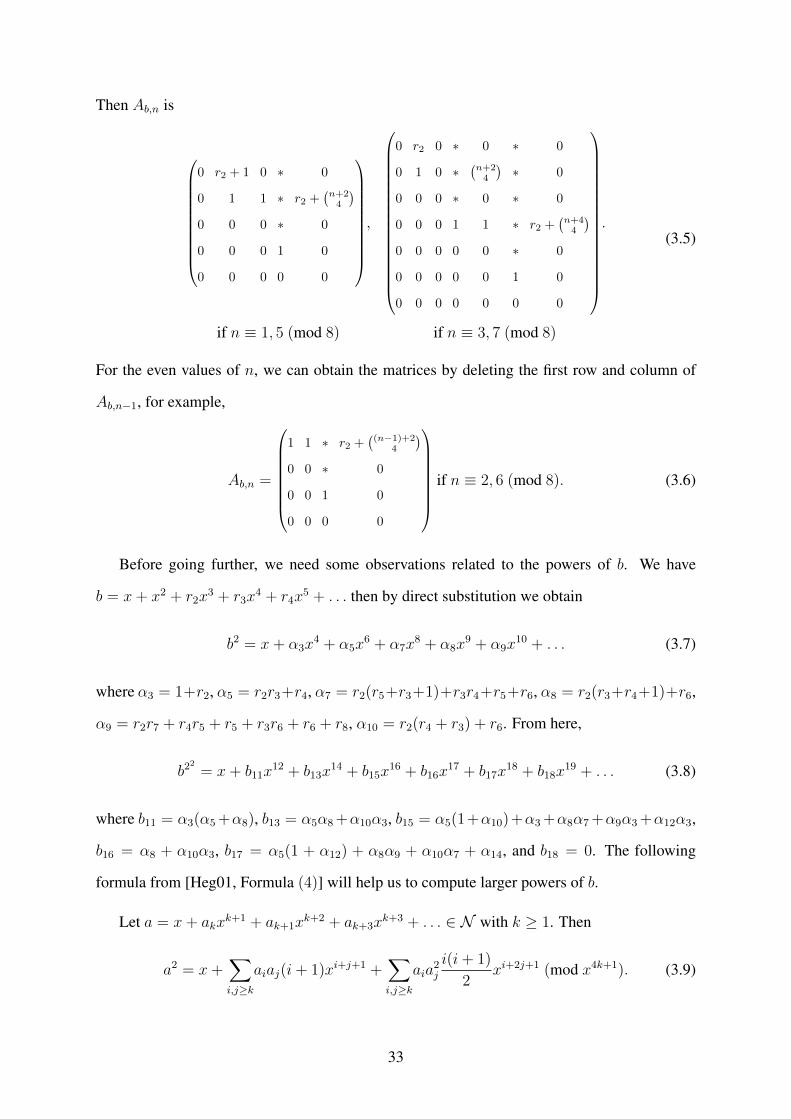
Then Ab,n is
0 r2 + 1 0 ∗ 0
0 1 1 ∗ r2 +(n+24
)0 0 0 ∗ 0
0 0 0 1 0
0 0 0 0 0
,
0 r2 0 ∗ 0 ∗ 0
0 1 0 ∗(n+24
)∗ 0
0 0 0 ∗ 0 ∗ 0
0 0 0 1 1 ∗ r2 +(n+44
)0 0 0 0 0 ∗ 0
0 0 0 0 0 1 0
0 0 0 0 0 0 0
.
if n ≡ 1, 5 (mod 8) if n ≡ 3, 7 (mod 8)
(3.5)
For the even values of n, we can obtain the matrices by deleting the first row and column of
Ab,n−1, for example,
Ab,n =
1 1 ∗ r2 +((n−1)+2
4
)0 0 ∗ 0
0 0 1 0
0 0 0 0
if n ≡ 2, 6 (mod 8). (3.6)
Before going further, we need some observations related to the powers of b. We have
b = x+ x2 + r2x3 + r3x
4 + r4x5 + . . . then by direct substitution we obtain
b2 = x+ α3x4 + α5x
6 + α7x8 + α8x
9 + α9x10 + . . . (3.7)
where α3 = 1+r2, α5 = r2r3+r4, α7 = r2(r5+r3+1)+r3r4+r5+r6, α8 = r2(r3+r4+1)+r6,
α9 = r2r7 + r4r5 + r5 + r3r6 + r6 + r8, α10 = r2(r4 + r3) + r6. From here,
b22 = x+ b11x12 + b13x
14 + b15x16 + b16x
17 + b17x18 + b18x
19 + . . . (3.8)
where b11 = α3(α5 +α8), b13 = α5α8 +α10α3, b15 = α5(1+α10)+α3 +α8α7 +α9α3 +α12α3,
b16 = α8 + α10α3, b17 = α5(1 + α12) + α8α9 + α10α7 + α14, and b18 = 0. The following
formula from [Heg01, Formula (4)] will help us to compute larger powers of b.
Let a = x+ akxk+1 + ak+1x
k+2 + ak+3xk+3 + . . . ∈ N with k ≥ 1. Then
a2 = x+∑i,j≥k
aiaj(i+ 1)xi+j+1 +∑i,j≥k
aia2j
i(i+ 1)
2xi+2j+1 (mod x4k+1). (3.9)
33

The following observation is a direct application of the formula (3.9).
Lemma 3.1.1. Let a = x +l∑
i=0
ak+2ixk+2i+1 +
∞∑j=2l+1
ak+jxk+j+1 where k is odd, l ∈ N, and
k ≥ 2l + 1 then
a2 = x+l+1∑i=1
cix2k+2l+2i +
∞∑j=1
cjx2k+4l+2+j.
In Lemma 3.1.1, the first odd power term in a is xk+2l+2. This causes a larger drop of the
depth of a2 than expected, that is, D(a2) ≥ 2k + 2l + 1 and the first odd power term in a2 is
x2k+4l+2+1.
Let us see an application of Lemma 3.1.1 which will give us the larger powers of our
b = x+x2+r2x3+r3x
4+r4x5+. . .. We have b22 = x+b11x
12+b13x14+b15x
16+b16x17+b17x
18+
b18x19 + . . ., here k = 11 = 24−5 and l = 2. ThenD(b23) ≥ 2(24−5)+2.2+1 = 25−5 = 27
and b23 = x+ c27x28 + c29x
30 + c31x32 + c32x
33 + . . .. Following this way, inductively we get
b2m = x+ αx2m+2−4 + βx2m+2−2 + γx2m+2
(mod x2m+2+1) (3.10)
for m ≥ 1, and for α, β, γ ∈ Fp (depending on m).
Now we have b2 = x + α3x4 + α5x
6 + α7x8 + α8x
9 + α9x10 + . . .. Let n be odd and
u1 = x + s0xn+1 + s1x
n+2 + s2xn+3 + . . .. We need to find the solution of b2u1[u1, b
2] ≡
u1b2 (mod xn+13) in order to find the coefficients of [u1, b
2] modulo (mod xn+13). Note that
the first term in b2u1 or b2u1[u1, b2], which may affect the solution of the equation above, is
2n + 5. If n ≥ 9 then 2n + 5 ≥ n + 13. Therefore, for n ≥ 9, we can write a general formula
(mod xn+13) to determine Ab2,n of size 9. Indeed,
u1b2 ≡ x+ α3x
4 + α5x6 + α7x
8 + α8x9 + . . .+ αn−1x
n + (s0 + αn)xn+1
+ (s1 + αn+1)xn+2 + (s2 + αn+2)xn+3 +
[s3 + αn+3 + (n+ 1)s0α3
]xn+4
+
[s4 + αn+4 + (n+ 2)s1α3
]xn+5 +
[s5 + αn+4 + (n+ 1)s0α5 + (n+ 3)s2α3
]xn+6
+
[s6 + αn+6 +
(n+1
2
)s0α3 + (n+ 2)s1α5 + (n+ 4)s3α3
]xn+7
+
[s7 + αn+7 + (n+ 1)s0α7 +
(n+2
2
)s1α3 + (n+ 3)s2α5 + (n+ 5)s4α3 +
]xn+8
34
+
[s8 + αn+8 + (n+ 1)s0α8 + (n+ 2)s1α7 +
(n+3
2
)s2α3 + (n+ 4)s3α5
+(n+ 6)s5α3
]xn+9
+
[s9 + αn+9 + (n+ 1)s0α9 +
(n+3
3
)s0α3 + (n+ 2)s1α8 + (n+ 3)s2α7
+(n+4
2
)s3α3 + (n+ 5)s4α5 + (n+ 7)s6α3
]xn+10
+
[s10 + α10 + (n+ 1)s0α10 +
(n+1
2
)s0α5 + (n+ 2)s1α9 +
(n+2
3
)s1α3 + (n+ 3)s2α8
+(n+ 4)s3α7 +(n+5
2
)s4α3 + (n+ 6)s5α5 + (n+ 8)s7α3
]xn+11
+
[s11 + αn+11 + (n+ 1)s0α11 +
(n+1
3
)s0α3α5 + (n+ 2)s1α10 +
(n+2
2
)s1α5
+(n+ 3)s2α9 +(n+3
3
)s2α3 + (n+ 4)s3α8 + (n+ 5)s4α7 +
(n+6
2
)s5α3
+(n+ 7)s6α5 + (n+ 9)s8α3
]xn+12 (mod xn+13)
b2u1 ≡ x+ α3x4 + α5x
6 + α7x8 + α8x
9 + . . .+ αn−1xn + (αn + s0)xn+1
+(αn+1 + s1)xn+2 + . . .+ (αn+7 + s7)xn+8 + (αn+8 + s8 + s0α8)xn+9
+(αn+9 + s9 + s1α8)xn+10 + (αn+10 + s10 + s2α8 + s0α10)xn+11
+(αn+11 + s11 + s3α8 + s1α10)xn+12 (mod xn+13)
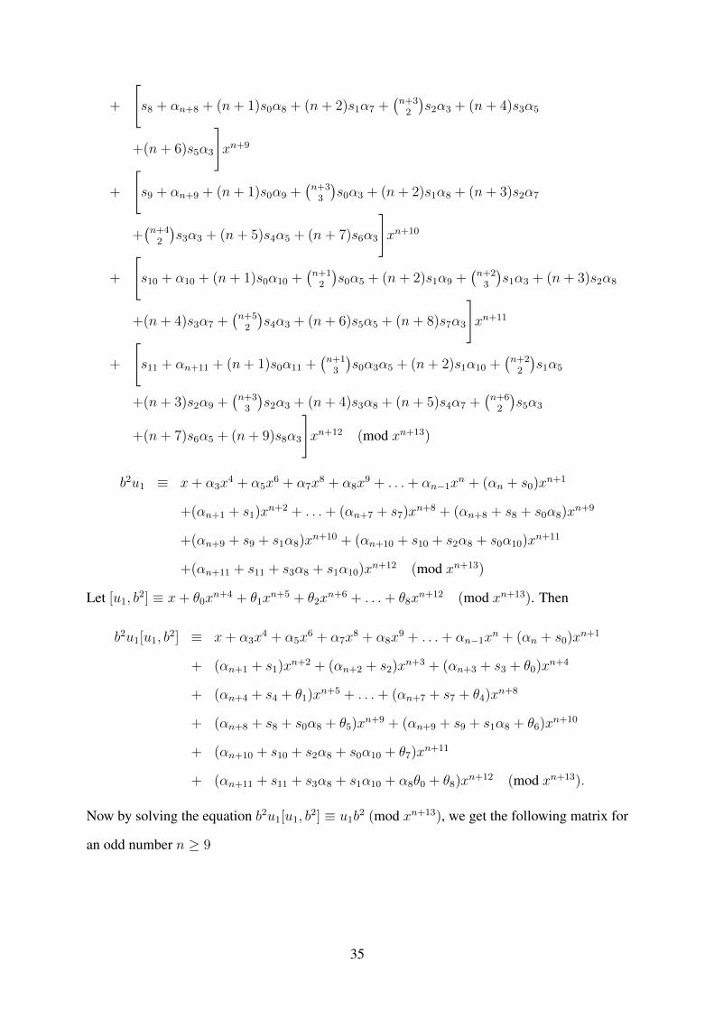
Let [u1, b2] ≡ x+ θ0x
n+4 + θ1xn+5 + θ2x
n+6 + . . .+ θ8xn+12 (mod xn+13). Then
b2u1[u1, b2] ≡ x+ α3x
4 + α5x6 + α7x
8 + α8x9 + . . .+ αn−1x
n + (αn + s0)xn+1
+ (αn+1 + s1)xn+2 + (αn+2 + s2)xn+3 + (αn+3 + s3 + θ0)xn+4
+ (αn+4 + s4 + θ1)xn+5 + . . .+ (αn+7 + s7 + θ4)xn+8
+ (αn+8 + s8 + s0α8 + θ5)xn+9 + (αn+9 + s9 + s1α8 + θ6)xn+10
+ (αn+10 + s10 + s2α8 + s0α10 + θ7)xn+11
+ (αn+11 + s11 + s3α8 + s1α10 + α8θ0 + θ8)xn+12 (mod xn+13).
Now by solving the equation b2u1[u1, b2] ≡ u1b
2 (mod xn+13), we get the following matrix for
an odd number n ≥ 9
35

Ab2,n =
0 0 0(n+12
)α3 0 α8 0 ∗ 0
0 α3 0 α5
(n+22
)α3 α7 0 ∗
(n+22
)α5
0 0 0 0 0(n+32
)α3 0 ∗ 0
0 0 0 α3 0 α5
(n+42
)α3 ∗ 0
0 0 0 0 0 0 0 ∗ 0
0 0 0 0 0 α3 0 ∗(n+62
)α3
0 0 0 0 0 0 0 ∗ 0
0 0 0 0 0 0 0 α3 0
0 0 0 0 0 0 0 0 0
. (3.11)
Let n = 3, then
u1b2 ≡ x+ (α3 + s0)x4 + s1x
5 + (α5 + s2)x6 + s3x7 + (α7 + α3s1 + s4)x8 + (α8 + s5)x9
+ (α9 + α5s1 + α3s3 + s6)x10 + (α10 + s7)x11 + (α11 + α7s1 + α3s2 + α5s3 + α3s5 + s8)x12
+ (α12 + α8s1 + α3s3 + s9)x13 + (α13 + α9s1 + α7s3 + α5s5 + α3s7 + s10)x14
+ (α14 + α10s1 + α8s3 + s11)x15
+ (α15 + α3s0 + α11s1 + α5s2 + α9s3 + α3s3 + α7s5 + α3s6 + α5s7 + α3s9 + s12)x16
+ (α16 + α12s1 + α3s1 + α10s3 + α5s3 + α8s5 + α3s7 + s13)x17
+ (α17 + α13s1 + α3s2 + α11s3 + α3α5s3 + α9s5 + α7s7 + α5s9 + α3s11 + s14)x18
+ (α18 + α14s1 + α12s3 + α3s3 + α10s5 + α8s7 + s15)x19
+ (α19 + α15s1 + α3s1 + α7s2 + α13s3 + α7α3s3 + α5α3s3 + α11s5
+α5s6 + α9s7 + α3s7 + α7s9 + α3s10 + α5s11 + α3s13 + s16)x20 (mod x21)
b2u1 ≡ x+ (α3 + s0)x4 + s1x5 + (α5 + s2)x6 + s3x
7 + (α7 + s4)x8 + (α8 + s5)x9
+ (α9 + s6)x10 + (α10 + s7)x11 + (α11 + α5s0 + α8s0 + s8)x12
+ (α12 + α8s1 + s9)x13 + (α13 + α5s1 + α8s2 + α10s0 + s10)x14
+ (α14 + α10s1 + α8s3 + s11)x15
+ (α15 + α3s0 + α5s2 + α8s4 + α9s0 + α10s2 + α12s0 + s12)x16
+ (α16 + α12s1 + α10s3 + α8s5 + α10s0 + s13)x17
+ (α17 + α5s3 + α5s0 + α8s6 + α9s1 + α10s4 + α12s2 + α14s0 + s14)x18
36

+ (α18 + α14s1 + α12s3 + α10s5 + α8s7 + α10s1 + s15)x19
+ (α19 + α3s1 + α5s4 + α8s8 + α9s2 + α10s6 + α10s0 + α12s4
+α13s0 + α14s3 + α16s0 + s16)x20 (mod x21).
Let [u1, b2] ≡ x+ x7θ0 + x8θ1 + x9θ2 + . . .+ x20θ13 (mod x21). Then
b2u1[u1, b2] ≡ x+ (α3 + s0)x4 + s1x
5 + (α5 + s2)x6 + (θ0 + s3)x7 + (θ1 + α7 + s4)x8
+ (θ2 + α8 + s5)x9 + (θ3 + α9 + s6)x10 + (θ4 + s1θ0 + α10 + s7)x11
+ (θ5 + s1θ1 + α11 + α5s0 + α8s0 + s8)x12 + (θ6 + s1θ2 + s3θ0 + α12 + α8s1 + s9)x13
+ (θ7 + s1θ3 + s3θ1 + α13 + α5s1 + α8s2 + α10s0 + s10)x14
+ (θ8 + s1θ4 + s3θ2 + (α8 + s5)θ0 + α14 + α10s1 + α8s3 + s11)x15
+(θ9 + s1θ5 + s3θ3 + (α8 + s5)θ1 + α15 + α3s0
+ α5s2 + α8s4 + α9s0 + α10s2 + α12s0 + s12
)x16
+(θ10 + s1θ6 + s3θ4 + (α8 + s5)θ2 + (α10 + s7)θ0
+ α16 + α12s1 + α10s3 + α8s5 + α10s0 + s13
)x17
+(θ11 + s1θ7 + (α5 + s2)θ0 + s3θ5 + (α8 + s5)θ3 + (α10 + s7)θ1
+ α17 + α5s3 + α5s0 + α8s6 + α9s1 + α10s4 + α12s2 + α14s0 + s14
)x18
+(θ12 + s1θ8 + s3θ6 + s3θ0 + (α8 + s5)θ4 + (α10 + s7)θ2 + (α12 + α8s1 + s9)θ0
+ α18 + α14s1 + α12s3 + α10s5 + α8s7 + α10s1 + s15
)x19
+(θ13 + s1θ9 + (α5 + s2)θ1 + s3θ7 + (α8 + s5)θ5
+ (α10 + s7)θ3 + (α12 + α8s1 + s3)θ1 + α19
+ α3s1 + α5s4 + α8s8 + α9s2 + α10s6 + α10s0
+ α12s4 + α13s0 + α14s3 + α16s0 + s16
)x20 (mod x21).
Now by solving the equation b2u1[u1, b2] ≡ u1b
2 (mod x21), we can get the matrix Ab2,3 of
size 14. Then we can obtain the matrix Ab2,n+2 from the matrix Ab2,n by deleting the first
two rows and columns of Ab2,n for n = 3, 5. We need only the upper left 9 × 9 corners
of Ab2,3, Ab2,5, Ab2,7. The form of the matrices is almost similar as in the case n ≥ 9. The
37
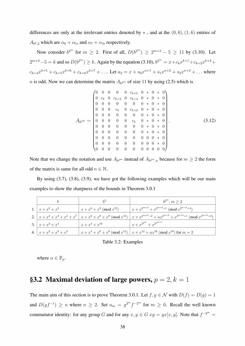
differences are only at the irrelevant entries denoted by ∗ , and at the (0, 6), (1, 6) entries of
Ab2,3 which are α8 + α5, and α7 + α3, respectively.
Now consider b2m for m ≥ 2. First of all, D(b2m) ≥ 2m+2 − 5 ≥ 11 by (3.10). Let
2m+2−5 = k and soD(b2m) ≥ k. Again by the equation (3.10), b2m = x+ckxk+1+ck+2x
k+3+
ck+4xk+5 + ck+5x
k+6 + ck+6xk+7 + . . .. Let u2 = x+ s0x
n+1 + s1xn+2 + s2x
n+3 + . . . where
n is odd. Now we can determine the matrix Ab2m of size 11 by using (2.5) which is
Ab2m =
0 0 0 0 0 ck+5 0 ∗ 0 ∗ 0
0 ck 0 ck+2 0 ck+4 0 ∗ 0 ∗ 0
0 0 0 0 0 0 0 ∗ 0 ∗ 0
0 0 0 ck 0 ck+2 0 ∗ 0 ∗ 0
0 0 0 0 0 0 0 ∗ 0 ∗ 0
0 0 0 0 0 ck 0 ∗ 0 ∗ 0
0 0 0 0 0 0 0 ∗ 0 ∗ 0
0 0 0 0 0 0 0 ∗ 0 ∗ 0
0 0 0 0 0 0 0 0 0 ∗ 0
0 0 0 0 0 0 0 0 0 ∗ 0
0 0 0 0 0 0 0 0 0 0 0
. (3.12)
Note that we change the notation and use Ab2m instead of Ab2m ,n because for m ≥ 2 the form
of the matrix is same for all odd n ∈ N.
By using (3.7), (3.8), (3.9), we have got the following examples which will be our main
examples to show the sharpness of the bounds in Theorem 3.0.1
b b2 b2m , m ≥ 2
1. x+ x2 + x3 x+ x8 + x9 (mod x12) x+ x2m+2+ x2m+2+1 (mod x2m+2+4)
2. x+ x2 + x3 + x4 + x7 x+ x6 + x8 + x9 (mod x12) x+ x2m+2−2 + αx2m+2+ x2m+2+1 (mod x2m+2+2)
3. x+ x2 + x4 x+ x4 + x16 x+ x22m
+ x22m+1
4. x+ x2 + x4 + x5 x+ x4 + x6 + x8 (mod x12) x+ x12 + αx16 (mod x18) for m = 2
Table 3.2: Examples
where α ∈ Fp.
§3.2 Maximal deviation of large powers, p = 2, k = 1
The main aim of this section is to prove Theorem 3.0.1. Let f, g ∈ N with D(f) = D(g) = 1
and D(gf−1) ≥ n where n ≥ 2. Set um = g2mf−2m for m ≥ 0. Recall the well known
commutator identity: for any group G and for any x, y ∈ G xy = yx[x, y]. Note that f−2m =
38

g−2mum. By taking square of both sides and using the commutator identity, we get
g2m+1
f−2m+1
= u2m[um, g
−2m ][[um, g−2m ], um]. (3.13)
Let m ≥ 0, denote by ~νm the coefficient vector of um. For m = 0, denote ~ν = ~ν0, and
u = u0. Let D(u2m) ≥ Bm, D([um, g
−2m ]) ≥ Cm, and D([[um, g−2m ], um]) ≥ Em. Let
Mm = min{Bm, Cm, Em}, and a ∈ {u2m, [um, g
−2m ], [[um, g−2m ], um]}. Let ~νm,a denote the
vector consisting of the coefficients of the terms xMm+i in a for i ≥ 0.
Remark 3.2.1. Let m ≥ 0 and suppose that D(um) ≥ 7. Then D([[um, g−2m ], um]) ≥
D([um, g−2m ]) + 7 by Proposition 1.2.3. It follows that
g2m+1
f−2m+1 ≡ u2m[um, g
−2m ] (mod xD([um,g−2m ])+8).
Remark 3.2.2. Suppose that D([u, g−1]) ≥ n + e(1, n) + 1 and n ≥ 7. By Proposition 1.2.3,
we have D(u2) ≥ 2n+e(1, n) ≥ n+e(1, n)+1+6 and D([[u, g−1], u]) ≥ n+e(1, n)+1+7.
Therefore, by (3.13), D(g2f−2) ≥ n+ e(1, n) + 1 and
D(g2f−2) ≡ [u, g−1] (mod xn+e(1,n)+7).
Let ~ν = (s0, s1, s3, . . .) and g−1 = x + x2 + r2x3 + r3x
4 + r4x5 + . . .. Throughout the
proof instead of over complicating the notation we will useC∗ to denote an undetermined value
which is 0 if C = 0, or we will use only ∗ when C is not important.
The following is a key observation of our proof:
Lemma 3.2.1. Let m ≥ 2, and n ≥ 2 arbitrary. Suppose that ~νm = (∗, 0, ∗, 0, ∗, ∗, . . . , ∗) and
D(um) ≥ n+e(1, n)+2m+2−K, where K ∈ {7, 9, 11} as in Theorem 3.0.1 (e.g., for n = 3, 4
K = 9 if m = 2, K = 7 if m ≥ 3 and so on). Then
D(um+1) = D(g2m+1
f−2m+1
) ≥ n+ e(1, n) + 2m+3 −K, ~νm+1 = (∗, 0, ∗, 0, ∗, ∗, . . . , ∗).
Equality holds if D(um) = n+ e(1, n) + 2m+2 −K, and one of the followings is satisfied:
(a) n = 2, m ≥ 2, ~νm = (1, 0, ∗, 0, ∗, 0, ∗, ∗, . . . , ∗), and (0, 6) entry of Ag−2m is 1,
39
(b) n = 3, 4, 5, 6, ~νm = (1, 0, ∗, 0, ∗, 0, ∗, ∗, . . . , ∗), m ≥ 3, the (0, 6) entry of Ag−2m is 1 for
m ≥ 2, and the (5, 6) entry of Ag−23 is 0,
(c) n ≥ 7, ~νm = (1, 0, ∗, 0, ∗, 0, ∗, ∗, . . . , ∗), m ≥ 2, the (0, 6) entry of Ag−2m is 1 for m ≥ 2,
and the (5, 6) entry of Ag−22 is 0.
Proof. First, note that by (3.10) we have D(g−2m) ≥ 2m+2 − 5. Then, by the matrix at (3.12),
~νmAg−2m = (0, 0, 0, 0, 0, ∗, 0, ∗, 0, ∗, 0) =⇒
D([um, g−2m ]) ≥ n+ e(1, n) + 2m+2 −K + 2m+2 − 5 + 5
= n+ e(1, n) + 2m+3 −K. (3.14)
On the other hand, D(u2m) ≥ 2(n+ e(1, n) + 2m+2 −K) + 5 ≥ n+ e(1, n) + 2m+3 −K, and
~νm+1,u2m= (∗, 0, ∗, 0, ∗, ∗, . . . , ∗) by Lemma 3.1.1. Also, by (3.14), we have ~νm+1,[um,g−2m ] =
(∗, 0, ∗, 0, ∗, 0, ∗, ∗, . . . , ∗). Then by Remark 3.2.1,
~νm+1 = (∗, 0, ∗, 0, ∗, ∗, . . . , ∗), D(um+1) ≥ n+ e(1, n) + 2m+3 −K.
Essentially, a similar proof implies our claim about equality. Indeed, for all the cases
(a), (b), (c) above, we have ~νm+1,[um,g−2m ] = (1, 0, ∗, 0, ∗, 0, ∗, ∗, . . . , ∗), and ~νm+1,u2m=
(0, 0, ∗, 0, ∗, 0, ∗, ∗, . . . , ∗). So we have ~νm+1 = (1, 0, ∗, 0, ∗, 0, ∗, ∗, . . . , ∗).
For the small values of n we do not have a regular formulation for the corresponding ma-
trices, so we have to investigate case by case. Hence, we first look at the general cases, that
is, when n ≥ 7. Then we look at the small values of n. We divide our proof into cases corre-
sponding to the different values of n modulo 8 since we have different matrices corresponding
to in these cases.
n ≥ 7 :
First we determine ~ν2 and D(u2) for each of n ≡ 1, 3, 5, 7 (mod 8).
n ≡ 1 (mod 8) : By using the first matrix at (3.5), and Remark 3.2.2,
~νAg−1,n = (0, ∗, ∗, ∗, r2∗) ⇒ D([u, g−1]) ≥ n+D(g−1) + 1 ≥ n+ 2 ≡ 3 (mod 8),
40
⇒ D(u1) = D(g2f−2) ≥ n+ 2, ~ν1 = (∗, ∗, ∗, r2∗, ∗, . . . , ∗).
Now by using (3.7) we have g−2 = x+α3x4 +α5x
6 +α7x8 +α8x
9 +α9x10 + . . ., and α3r2 = 0.
By using the matrix at (3.11), Remark 3.2.1 and Proposition 1.2.3,
~ν1Ag−2,n+2 = (0, α3∗, 0, α5 ∗+α3∗, 0, ∗, α3r2∗, ∗, 0) = (0, α3∗, 0, ∗, 0, ∗, 0, ∗, 0, ∗, . . . , ∗)
⇒ D([u1, g−2]) ≥ n+ 2 +D(g−2) + 1 ≥ n+ 2 + 3 + 1 = n+ 6 = n+ e(1, n) + 24 − 11.
D(u21) ≥ 2(n+ 2) + 1 ≥ n+ 6 + n− 1 ≥ n+ 6 + 8.
⇒ D(u2) = D(g22f−22) ≥ n+6 = n+e(1, n)+24−11, ~ν2 = (α3∗, 0, ∗, 0, ∗, 0, ∗, 0, ∗, . . . , ∗).
n ≡ 3 (mod 8) : By using the second matrix at (3.5) and Remark 3.2.2,
~νAg−1,n = (0, ∗, 0, ∗, ∗, ∗, ∗)⇒ D([u, g−1]) ≥ n+ 1 + 1 ≡ 5 (mod 8),
⇒ D(u1) = D(g2f−2) ≥ n+ 2, ~ν1 = (∗, 0, ∗, ∗, ∗, ∗, .., ∗).
By using the matrix at (3.11), Lemma 3.1.1 and Remark 3.2.1,
~ν1Ag−2,n+2 = (0, 0, 0, α3∗, 0, ∗, 0, ∗, α3∗)
⇒ D([u1, g−2]) ≥ n+ 2 + 3 + 3 = n+ 8 = n+ e(1, n) + 24 − 9.
D(u21) ≥ 2(n+ 2) + 3 ≥ n+ 8 + 10.
⇒ D(u2) = D(g22f−22) ≥ n+ 8 = n+ e(1, n) + 24 − 9, ~ν2 = (α3∗, 0, ∗, 0, ∗, α3∗, ∗, . . . , ∗).
n ≡ 5 (mod 8) : By using the first matrix at (3.5) and Remark 3.2.2,
~νAg−1,n = (0, ∗, ∗, ∗, ∗)⇒ D([u, g−1]) ≥ n+ e(1, n) + 1 ≡ 7 (mod 8)
⇒ D(u1) = D(g2f−2) ≥ n+ 2, ~ν1 = (∗, ∗, , . . . , ∗).
By using the matrix at (3.11), Remark 3.2.1 and Proposition 1.2.3,
~ν1Ag−2,n+2 = (0, α3∗, 0, ∗, 0, ∗, α3∗, ∗, 0)
⇒ D([u1, g−2]) ≥ n+ 2 + 3 + 1 = n+ 6 = n+ e(1, n) + 24 − 11.
41
D(u21) ≥ 2(n+ 2) + 1 ≥ n+ 6 + 12.
⇒ D(u2) = D(g22f−22) ≥ n+ e(1, n) + 24 − 11, ~ν2 = (α3∗, 0, ∗, 0, ∗, α3∗, ∗, 0, ∗, ∗, . . . , ∗).
n ≡ 7 (mod 8) : By using the second matrix at (3.5) and Remark 3.2.2,
~νAg−1,n = (0, ∗, 0, ∗, ∗, ∗, r2∗)⇒ D([u, g−1]) ≥ n+ 2 ≡ 1 (mod 8).
⇒ D(u1) = D(g2f−2) ≥ n+ 2, ~ν1 = (∗, 0, ∗, ∗, ∗, r2∗, ∗, ∗, . . . , ∗).
By using the matrix at (3.11), Lemma 3.1.1 and Remark 3.2.1,
~ν1Ag−2,n+2 = (0, 0, 0, α3∗, 0, ∗, 0, ∗, α3r2∗) = (0, 0, 0, α3∗, 0, ∗, 0, ∗, 0) (as α3r2 = 0)
⇒ D([u1, g−2]) ≥ n+ 2 + 3 + 3 = n+ e(1, n) + 24 − 9.
D(u21) ≥ 2(n+ 2) + 3 ≥ n+ 8 + 6.
⇒ D(u2) = D(g2f−2) ≥ n+ e(1, n) + 24 − 9, ~ν2 = (α3∗, 0, ∗, 0, ∗, 0, ∗, ∗, . . . , ∗).
Now we have the vector ~ν2 = (α3∗, 0, ∗, 0, ∗, δα3∗, ∗, ∗, . . . , ∗), where δ = 0 if n ≡
1, 7 (mod 8) and δ = 1 if n ≡ 3, 5 (mod 8). Also D(u2) ≥ n + e(1, n) + 24 − K, where
K = 11 if n ≡ 1, 5 (mod 8), K = 9 if n ≡ 3, 7 (mod 8).
Suppose that α3 = 1 then by using (3.7), (3.8) and (3.9), the coefficients of the terms x17
in b22 and x32 in b23 are both zero. So (0, 6) entry of the matrix at (3.12) is zero for m = 2, 3.
Thus,
~ν2Ag−22 = (0, 0, 0, 0, 0, δ∗, 0, ∗, 0, ∗, 0)⇒ D([u2, g−22 ]) ≥ n+ e(1, n) + 25 −K + λ
where λ = 2 if δ = 0, λ = 0 otherwise . On the other hand, by Lemma 3.1.1, D(u22) ≥ 2(n +
e(1, n)+24−K)+5+λ ≥ n+e(1, n)+25−K+4+λ and ~ν3,u22= (0, 0, 0, 0, ∗, 0, ∗, ∗, . . . , ∗).
Now by Remark 3.2.1,
~ν3 = (δ∗, 0, ∗, 0, ∗, 0, ∗, ∗, . . . , ∗), D(u3) ≥ n+ e(1, n) + 25 −K + λ.
Above we noted that (0, 6) entry of the matrix at (3.12) is zero for m = 3 so
~ν3Ag−23 = (0, 0, 0, 0, 0, 0, 0, ∗, 0, ∗, 0), D([u3, g−23 ]) ≥ n+ e(1, n) + 26 −K + λ+ 2.
42
On the other hand, by Lemma 3.1.1, D(u23) ≥ 2(n+ e(1, n) + 25−K+λ) + 7 ≥ n+ e(1, n) +
26 −K + λ+ 2 + 6. By Remark 3.2.1
~ν4 = (∗, 0, ∗, 0, ∗, ∗, . . . , ∗), D(u4) ≥ n+ e(1, n) + 26 −K + λ+ 2.
Here we can apply Lemma 3.2.1 with an inductive argument to getD(g2mf−2m) ≥ n+e(1, n)+
2m+2 −K + λ+ 2 for m ≥ 4.
Now suppose that α3 = 0 then ~ν2 = (∗, 0, ∗, 0, ∗, ∗, . . . , ∗) and D(u2) ≥ n+ e(1, n) + 24−
K + 2. Now we can apply Lemma 3.2.1 with an inductive argument to get D(g2mf−2m) ≥
n+ e(1, n) + 2m+2 −K + 2 for m ≥ 2.
Now we have
D(g2mf−2m) ≥
n+ e(1, n) + 2m+2 −K if m = 2,
n+ e(1, n) + 2m+2 −K + 2 if m ≥ 3.
(3.15)
D(g2mf−2m) ≥
n+ e(1, n) + 2m+2 −K ′ if m = 2, 3,
n+ e(1, n) + 2m+2 −K ′ + 2 if m ≥ 4.
(3.16)
where K,K ′ = 11 if n ≡ 1 (mod 8), n ≡ 5 (mod 8), respectively, and K,K ′ = 9 if
n ≡ 7 (mod 8), n ≡ 3 (mod 8), respectively. This confirms the bound of Theorem 3.0.1 in this
case.
n ≡ 2,4,6,8 : The case of an even n ≥ 8 is closely related to its odd counterpart
n− 1, above. We see that ~νAg−1 is exactly the same vector as ~ν1 obtained for n− 1, above. On
the other hand, D(u1) = n + e(1, n) + 1 = n − 1 + e(1, n − 1) + 1 as n is even. From now
on the proof is the same as for n− 1, above, so are the bounds. Now return to the sharpness of
the bounds.
43

Example for n ≡ 1,2,5,6 (mod 8) :
m ≤ 3 : Let n ≡ 1, 5 (mod 8) and g−1 = x + x2 + x4 + x5. We have the following matrices
by using the matrices at (3.5), (3.11), (3.12), and example 4 in Table 3.2
Ag−1,n =
0 1 0 ∗ 0
0 1 1 ∗(n+24
)0 0 0 ∗ 0
0 0 0 ∗ 0
0 0 0 0 0
, Ag−2m =
0 0 0 0 0 0 0 ∗ 0
0 1 0 ∗ 0 ∗ 0 ∗ 0
0 0 0 0 0 ε 0 ∗ 0
0 0 0 1 0 ∗ ε ∗ 0
0 0 0 0 0 0 0 ∗ 0
0 0 0 0 0 1 0 ∗ 0
0 0 0 0 0 0 0 ∗ 0
0 0 0 0 0 0 0 1 0
0 0 0 0 0 0 0 0 0
(3.17)
where m = 1, 2. Also ε = 1 if m = 1, zero otherwise. Let ~ν = (1, 1, ∗, ∗, . . . , ∗)
then ~νAg−1,n = (0, 0, 1, ∗,(n+2
4
)). Now ~ν1 = (0, 1, ∗,
(n+2
4
), ∗, ∗, . . . , ∗). It follows that
~ν1Ag−2,n+2 = (0, 1, 0, ∗, 0, ∗,(n+2
4
), ∗, 0) and so D(g22f−22) = n + e(1, n) + 24 − 11.
Hence, for m = 2 and n ≡ 1, 5 (mod 8) we have the desired bound. Now suppose
n ≡ 5 (mod 8) then(n+2
4
)= 1. So we have ~ν2 = (1, 0, ∗, 0, ∗, 1, ∗, 0, ∗, ∗, . . . , ∗). Thus,
~ν2Ag−22 = (0, 0, 0, 0, 0, 1, 0, ∗, 0) and so we have D(g23f−23) = n + e(1, n) + 25 − 11, which
is the desired bound for n ≡ 5 (mod 8). For the even values n ≡ 2, 6 (mod 8), it can be directly
seen that the same example produces the desired bound which is same as for n ≡ 1, 5 (mod 8).
Indeed, from ~νAg−1,n we get ~ν1 = (1, 1, ∗,(n+1
4
)) which produces same ~ν2 and D(u2) as in the
odd case.
m ≥ 3 :Let n ≡ 1, 5 (mod 8) and g−1 = x + x2 + x3 + x4 + x7. By using the matri-
ces at (3.5), (3.11), (3.12), and example 2 in Table 3.2,
Ag−1,n =
0 0 0 ∗ 0
0 1 1 ∗(n+24
)0 0 0 ∗ 0
0 0 0 ∗ 0
0 0 0 0 0
, Ag−2m =
0 0 0 0 0 1 0 ∗ 0
0 0 0 1 0 ∗ 0 ∗ 0
0 0 0 0 0 0 0 ∗ 0
0 0 0 0 0 1 0 ∗ 0
0 0 0 0 0 0 0 ∗ 0
0 0 0 0 0 0 0 ∗ 0
0 0 0 0 0 0 0 ∗ 0
0 0 0 0 0 0 0 1 0
0 0 0 0 0 0 0 0 0
. (3.18)
44
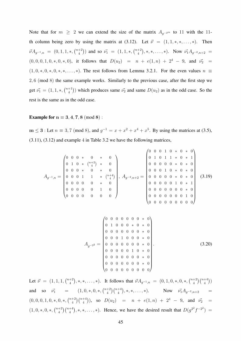
Note that for m ≥ 2 we can extend the size of the matrix Ag−2m to 11 with the 11-
th column being zero by using the matrix at (3.12). Let ~ν = (1, 1, ∗, ∗, . . . , ∗). Then
~νAg−1,n = (0, 1, 1, ∗,(n+2
4
)) and so ~ν1 = (1, 1, ∗,
(n+2
4
), ∗, ∗, . . . , ∗). Now ~ν1Ag−2,n+2 =
(0, 0, 0, 1, 0, ∗, 0, ∗, 0), it follows that D(u2) = n + e(1, n) + 24 − 9, and ~ν2 =
(1, 0, ∗, 0, ∗, 0, ∗, ∗, . . . , ∗). The rest follows from Lemma 3.2.1. For the even values n ≡
2, 6 (mod 8) the same example works. Similarly to the previous case, after the first step we
get ~ν1 = (1, 1, ∗,(n+1
4
)) which produces same ~ν2 and same D(u2) as in the odd case. So the
rest is the same as in the odd case.
Example for n ≡ 3,4,7,8 (mod 8) :
m ≤ 3 : Let n ≡ 3, 7 (mod 8), and g−1 = x + x2 + x4 + x5. By using the matrices at (3.5),
(3.11), (3.12) and example 4 in Table 3.2 we have the following matrices,
Ag−1,n =
0 0 0 ∗ 0 ∗ 0
0 1 0 ∗(n+24
)∗ 0
0 0 0 ∗ 0 ∗ 0
0 0 0 1 1 ∗(n+44
)0 0 0 0 0 ∗ 0
0 0 0 0 0 1 0
0 0 0 0 0 0 0
, Ag−2,n+2 =
0 0 0 1 0 ∗ 0 ∗ 0
0 1 0 1 1 ∗ 0 ∗ 1
0 0 0 0 0 ∗ 0 ∗ 0
0 0 0 1 0 ∗ 0 ∗ 0
0 0 0 0 0 ∗ 0 ∗ 0
0 0 0 0 0 1 0 ∗ 1
0 0 0 0 0 0 0 ∗ 0
0 0 0 0 0 0 0 1 0
0 0 0 0 0 0 0 0 0
(3.19)
Ag−22 =
0 0 0 0 0 0 0 ∗ 0
0 1 0 0 0 ∗ 0 ∗ 0
0 0 0 0 0 0 0 ∗ 0
0 0 0 1 0 0 0 ∗ 0
0 0 0 0 0 0 0 ∗ 0
0 0 0 0 0 1 0 ∗ 0
0 0 0 0 0 0 0 ∗ 0
0 0 0 0 0 0 0 ∗ 0
0 0 0 0 0 0 0 0 0
. (3.20)
Let ~ν = (1, 1, 1,(n+2
4
), ∗, ∗, . . . , ∗). It follows that ~νAg−1,n = (0, 1, 0, ∗, 0, ∗,
(n+2
4
)(n+4
4
))
and so ~ν1 = (1, 0, ∗, 0, ∗,(n+2
4
)(n+4
4
), ∗, ∗, . . . , ∗). Now ~ν1Ag−2,n+2 =
(0, 0, 0, 1, 0, ∗, 0, ∗,(n+2
4
)(n+4
4
)), so D(u2) = n + e(1, n) + 24 − 9, and ~ν2 =
(1, 0, ∗, 0, ∗,(n+2
4
)(n+4
4
), ∗, ∗, . . . , ∗). Hence, we have the desired result that D(g22f−22) =
45
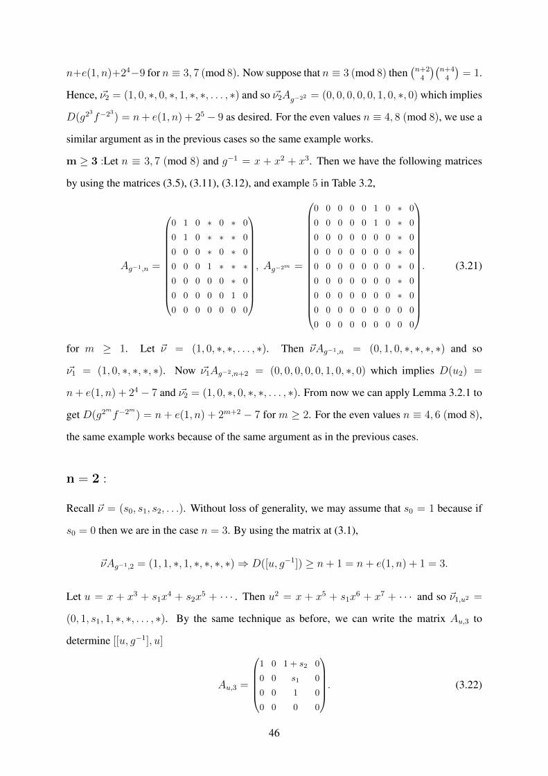
n+e(1, n)+24−9 for n ≡ 3, 7 (mod 8). Now suppose that n ≡ 3 (mod 8) then(n+2
4
)(n+4
4
)= 1.
Hence, ~ν2 = (1, 0, ∗, 0, ∗, 1, ∗, ∗, . . . , ∗) and so ~ν2Ag−22 = (0, 0, 0, 0, 0, 1, 0, ∗, 0) which implies
D(g23f−23) = n+ e(1, n) + 25 − 9 as desired. For the even values n ≡ 4, 8 (mod 8), we use a
similar argument as in the previous cases so the same example works.
m ≥ 3 :Let n ≡ 3, 7 (mod 8) and g−1 = x + x2 + x3. Then we have the following matrices
by using the matrices (3.5), (3.11), (3.12), and example 5 in Table 3.2,
Ag−1,n =
0 1 0 ∗ 0 ∗ 0
0 1 0 ∗ ∗ ∗ 0
0 0 0 ∗ 0 ∗ 0
0 0 0 1 ∗ ∗ ∗0 0 0 0 0 ∗ 0
0 0 0 0 0 1 0
0 0 0 0 0 0 0
, Ag−2m =
0 0 0 0 0 1 0 ∗ 0
0 0 0 0 0 1 0 ∗ 0
0 0 0 0 0 0 0 ∗ 0
0 0 0 0 0 0 0 ∗ 0
0 0 0 0 0 0 0 ∗ 0
0 0 0 0 0 0 0 ∗ 0
0 0 0 0 0 0 0 ∗ 0
0 0 0 0 0 0 0 0 0
0 0 0 0 0 0 0 0 0
. (3.21)
for m ≥ 1. Let ~ν = (1, 0, ∗, ∗, . . . , ∗). Then ~νAg−1,n = (0, 1, 0, ∗, ∗, ∗, ∗) and so
~ν1 = (1, 0, ∗, ∗, ∗, ∗). Now ~ν1Ag−2,n+2 = (0, 0, 0, 0, 0, 1, 0, ∗, 0) which implies D(u2) =
n+ e(1, n) + 24 − 7 and ~ν2 = (1, 0, ∗, 0, ∗, ∗, . . . , ∗). From now we can apply Lemma 3.2.1 to
get D(g2mf−2m) = n + e(1, n) + 2m+2 − 7 for m ≥ 2. For the even values n ≡ 4, 6 (mod 8),
the same example works because of the same argument as in the previous cases.
n = 2 :
Recall ~ν = (s0, s1, s2, . . .). Without loss of generality, we may assume that s0 = 1 because if
s0 = 0 then we are in the case n = 3. By using the matrix at (3.1),
~νAg−1,2 = (1, 1, ∗, 1, ∗, ∗, ∗, ∗)⇒ D([u, g−1]) ≥ n+ 1 = n+ e(1, n) + 1 = 3.
Let u = x + x3 + s1x4 + s2x
5 + · · · . Then u2 = x + x5 + s1x6 + x7 + · · · and so ~ν1,u2 =
(0, 1, s1, 1, ∗, ∗, . . . , ∗). By the same technique as before, we can write the matrix Au,3 to
determine [[u, g−1], u]
Au,3 =
1 0 1 + s2 0
0 0 s1 0
0 0 1 0
0 0 0 0
. (3.22)
46
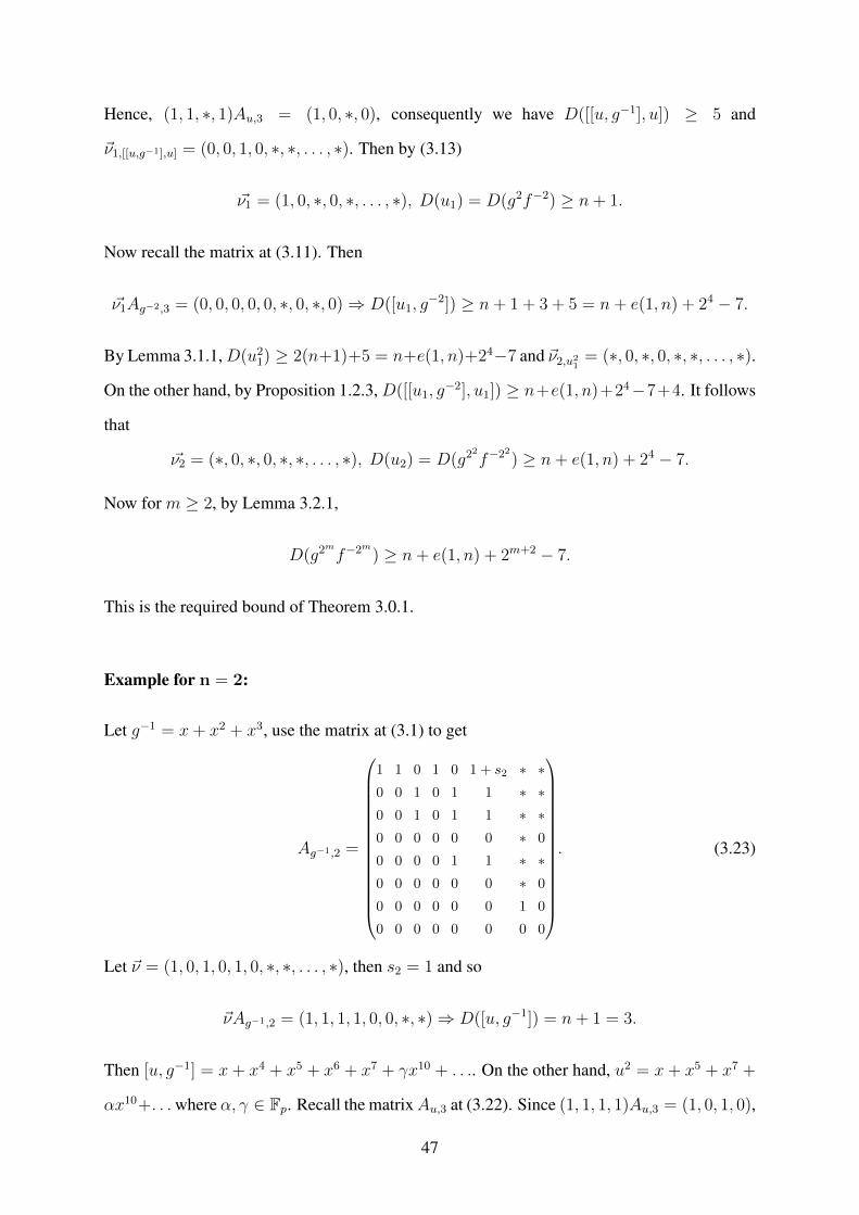
Hence, (1, 1, ∗, 1)Au,3 = (1, 0, ∗, 0), consequently we have D([[u, g−1], u]) ≥ 5 and
~ν1,[[u,g−1],u] = (0, 0, 1, 0, ∗, ∗, . . . , ∗). Then by (3.13)
~ν1 = (1, 0, ∗, 0, ∗, . . . , ∗), D(u1) = D(g2f−2) ≥ n+ 1.
Now recall the matrix at (3.11). Then
~ν1Ag−2,3 = (0, 0, 0, 0, 0, ∗, 0, ∗, 0)⇒ D([u1, g−2]) ≥ n+ 1 + 3 + 5 = n+ e(1, n) + 24 − 7.
By Lemma 3.1.1,D(u21) ≥ 2(n+1)+5 = n+e(1, n)+24−7 and ~ν2,u21
= (∗, 0, ∗, 0, ∗, ∗, . . . , ∗).
On the other hand, by Proposition 1.2.3, D([[u1, g−2], u1]) ≥ n+e(1, n)+24−7+4. It follows
that
~ν2 = (∗, 0, ∗, 0, ∗, ∗, . . . , ∗), D(u2) = D(g22f−22) ≥ n+ e(1, n) + 24 − 7.
Now for m ≥ 2, by Lemma 3.2.1,
D(g2mf−2m) ≥ n+ e(1, n) + 2m+2 − 7.
This is the required bound of Theorem 3.0.1.
Example for n = 2:
Let g−1 = x+ x2 + x3, use the matrix at (3.1) to get
Ag−1,2 =
1 1 0 1 0 1 + s2 ∗ ∗0 0 1 0 1 1 ∗ ∗0 0 1 0 1 1 ∗ ∗0 0 0 0 0 0 ∗ 0
0 0 0 0 1 1 ∗ ∗0 0 0 0 0 0 ∗ 0
0 0 0 0 0 0 1 0
0 0 0 0 0 0 0 0
. (3.23)
Let ~ν = (1, 0, 1, 0, 1, 0, ∗, ∗, . . . , ∗), then s2 = 1 and so
~νAg−1,2 = (1, 1, 1, 1, 0, 0, ∗, ∗)⇒ D([u, g−1]) = n+ 1 = 3.
Then [u, g−1] = x+ x4 + x5 + x6 + x7 + γx10 + . . .. On the other hand, u2 = x+ x5 + x7 +
αx10+. . .where α, γ ∈ Fp. Recall the matrixAu,3 at (3.22). Since (1, 1, 1, 1)Au,3 = (1, 0, 1, 0),
47
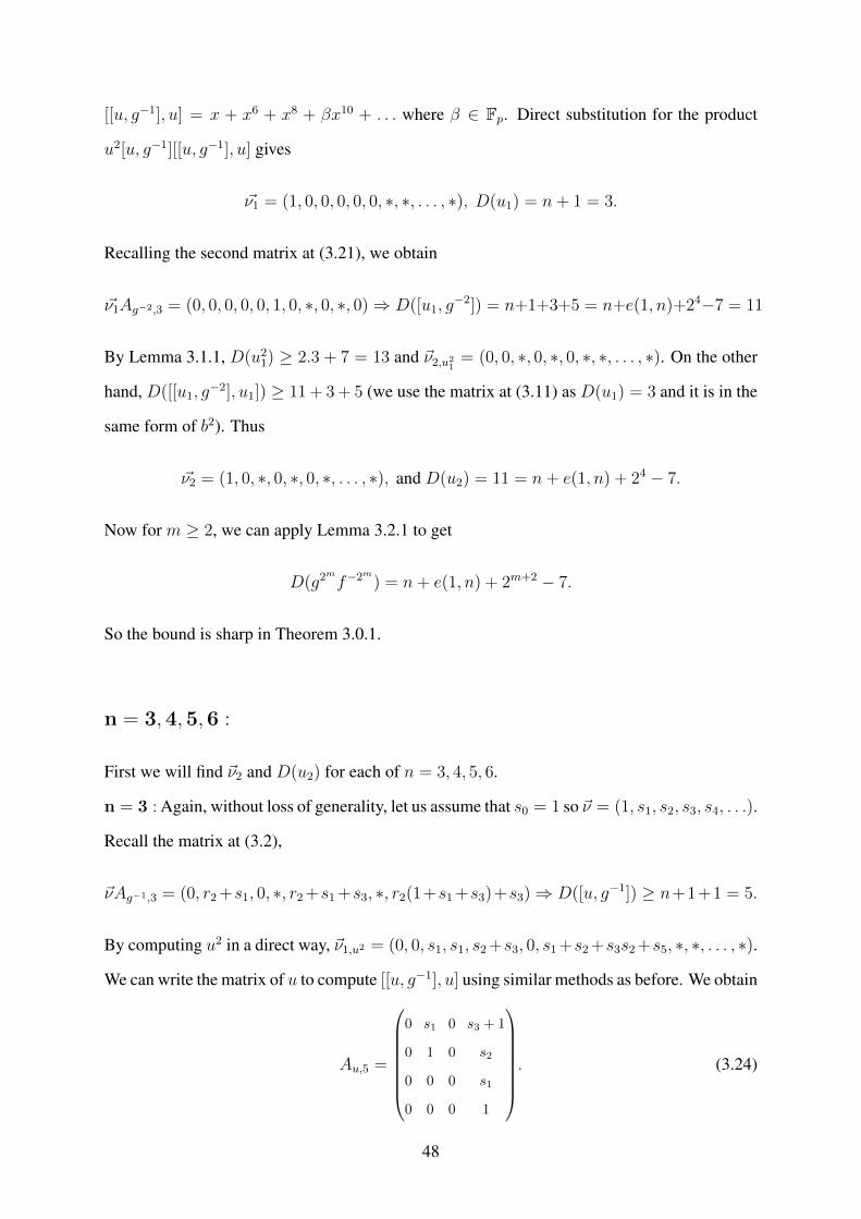
[[u, g−1], u] = x + x6 + x8 + βx10 + . . . where β ∈ Fp. Direct substitution for the product
u2[u, g−1][[u, g−1], u] gives
~ν1 = (1, 0, 0, 0, 0, 0, ∗, ∗, . . . , ∗), D(u1) = n+ 1 = 3.
Recalling the second matrix at (3.21), we obtain
~ν1Ag−2,3 = (0, 0, 0, 0, 0, 1, 0, ∗, 0, ∗, 0)⇒ D([u1, g−2]) = n+1+3+5 = n+e(1, n)+24−7 = 11
By Lemma 3.1.1, D(u21) ≥ 2.3 + 7 = 13 and ~ν2,u21
= (0, 0, ∗, 0, ∗, 0, ∗, ∗, . . . , ∗). On the other
hand, D([[u1, g−2], u1]) ≥ 11 + 3 + 5 (we use the matrix at (3.11) as D(u1) = 3 and it is in the
same form of b2). Thus
~ν2 = (1, 0, ∗, 0, ∗, 0, ∗, . . . , ∗), and D(u2) = 11 = n+ e(1, n) + 24 − 7.
Now for m ≥ 2, we can apply Lemma 3.2.1 to get
D(g2mf−2m) = n+ e(1, n) + 2m+2 − 7.
So the bound is sharp in Theorem 3.0.1.
n = 3,4,5,6 :
First we will find ~ν2 and D(u2) for each of n = 3, 4, 5, 6.
n = 3 : Again, without loss of generality, let us assume that s0 = 1 so ~ν = (1, s1, s2, s3, s4, . . .).
Recall the matrix at (3.2),
~νAg−1,3 = (0, r2 +s1, 0, ∗, r2 +s1 +s3, ∗, r2(1+s1 +s3)+s3)⇒ D([u, g−1]) ≥ n+1+1 = 5.
By computing u2 in a direct way, ~ν1,u2 = (0, 0, s1, s1, s2 +s3, 0, s1 +s2 +s3s2 +s5, ∗, ∗, . . . , ∗).
We can write the matrix of u to compute [[u, g−1], u] using similar methods as before. We obtain
Au,5 =
0 s1 0 s3 + 1
0 1 0 s2
0 0 0 s1
0 0 0 1
. (3.24)
48
Then ~ν1,[[u,g−1],u] = (0, 0, 0, 0, s1(r2 + s1), 0, ∗, ∗, . . . , ∗). Thus, by (3.13),
~ν1 = (r2 + s1, 0, ∗, r2 + s3, ∗, r2(1 + s1 + s3) + s3, ∗, ∗, . . . , ∗), D(u1) = D(g2f−2) ≥ n+ 2.
Recall the matrix at (3.11),
~ν1Ag−2,5 = (0, 0, 0, α3(s1 + s3), 0, ∗, 0, ∗, α3(r2(1 + s1 + s3) + s3))
⇒ D([u1, g−2]) ≥ n+ 2 + 3 + 3 = n+ e(1, n) + 24 − 9.
A direct computation gives the coefficient vector ~ν2,u21= (0, 0, (r2 + s3)(r2 + s1), 0, ∗, r2 +
s3, ∗, ∗, . . . , ∗) . On the other hand, by Proposition 1.2.3, D([[u1, g−2], u1]) ≥ n + e(1, n) +
24 − 9 + 6. Thus, by (3.13),
~ν2 = (α3(s1 + s3), 0, ∗, 0, ∗, r2α3(1 + s1 + s3) + r2 + (α3 + 1)s3, ∗, ∗, . . . , ∗),
D(u2) = D(g22f−22) ≥ n+ e(1, n) + 24 − 9.
Note that α3r2 = 0 by (3.7). So we have ~ν2 = (α3∗, 0, ∗, 0, ∗, r2∗, ∗, ∗, . . . , ∗).
n = 4 : Recall the matrix at (3.3), then
~νAg−1,4 = (1, 0, ∗, 1 + s2, ∗, r2(1 + s2) + s2)⇒ D([u, g−1]) ≥ n+ 1.
A direct computation gives ~ν1,u2 = (0, 0, 0, 1, s1, 0, ∗, ∗, . . . , ∗). On the other hand,
~ν1,[[u,g−1],u] = (0, 0, 0, 0, 1, 0, ∗, ∗, . . . , ∗) by using the matrix at (2.5). Now by (3.13),
~ν1 = (1, 0, ∗, s2, ∗, r2(1 + s2) + s2, ∗, ∗, . . . , ∗), D(u1) = D(g2f−2) ≥ n+ 1.
Recall the matrix at (3.11)
~ν1Ag−2,5 = (0, 0, 0, α3(1 + s2), 0, ∗, 0, ∗, α3(r2(1 + s2) + s2))
⇒ D([u1, g−2]) ≥ n+ 7 = n+ e(1, k) + 24 − 9.
On the other hand, ~ν2,u21= (0, 0, s2, 0, ∗, s2, ∗, ∗, . . . , ∗) by a direct computation, and
D([[u1, g−2], u1]) ≥ n+ 7 + 6 by Proposition 1.2.3. Then by (3.13),
~ν2 = (α3(1+s2), 0, ∗, 0, ∗, α3(r2(1+s2)+s2)+s2, ∗, ∗, . . . , ∗), D(g22f−22) ≥ n+e(1, n)+24−9.
49

Again, since r2α3 = 0 by (3.7), we have ~ν2 = (α3∗, 0, ∗, 0, ∗, r2∗, ∗, ∗, . . . , ∗).
n = 5: Let ~ν = (1, s1, s2, s3, . . .). Recall the first matrix at (3.4),
~νAg−2,5 = (0, r2 + 1 + s1, s1, ∗, (r2 + 1)s1)⇒ D([u, g−1]) ≥ n+ 2 = 7.
On the other hand, by Proposition 1.2.3, D(u2) ≥ 2.5 + 1 = 11 and so ~ν1,u2 = (0, 0, 0, 0, ∗, ∗).
Also D([[u, g−1], u]) ≥ 7 + 6 by Proposition 1.2.3. So by (3.13)
~ν1 = (r2 + s1 + 1, s1, ∗, (r2 + 1)s1, ∗, ∗, . . . , ∗), D(g2f−2) ≥ n+ 2.
Recall the matrix at (3.11), also recall α3 = 1 + r2 from (3.7), then
~ν1Ag−2,7 = (0, α3s1, 0, ∗, 0, ∗, α3s1, ∗, 0), D([u1, g−2]) ≥ n+2+1+3 = 11 = n+e(1, n)+24−11.
D(u21) ≥ 2.7 + 1 = 15 and ~ν2,u21
= (0, 0, 0, 0, s1r2, s1, ∗, ∗, . . . , ∗) by Proposition 1.2.3. So by
Remark 3.2.1, we have
~ν2 = (α3∗, 0, ∗, 0, ∗, (α3 + 1)∗, ∗, ∗, . . . , ∗), D(g22f−22) ≥ n+ e(1, n) + 24 − 11.
By (3.7), α3 = 1 + r2 so ~ν2 = (α3∗, 0, ∗, 0, ∗, r2∗, ∗, ∗, . . . , ∗).
n = 6: Recall the matrix at (3.4), delete its first row and column to get the matrix Ag−1,6. Then
~νAg−1,6 = (1, 1, ∗, r2 + 1, ∗, ∗, . . . , ∗), D([u, g−1]) ≥ n+ 1 = 7.
On the other hand, by using Proposition 1.2.3,D(u2) ≥ 2.6 = 7+5 andD([[u, g−1], u]) ≥ 7+6,
so we have
~ν1 = (1, 1, ∗, r2 + 1, ∗, ∗, . . . , ∗), D(g2f−2) ≥ n+ 1 = 7.
Now recall the matrix at (3.11). Also recall that α3 = 1 + r2, by (3.7), then
~ν1Ag−2,7 = (0, α3, 0, ∗, 0, ∗, α3, ∗, 0), D([u1, g−2]) ≥ n+1+3+1 = 11 = n+e(1, n)+24−11.
On the other hand, by Proposition 1.2.3 and a direct computation, D(u21) ≥ 2.7 + 1 and ~ν2,u21
=
(0, 0, 0, 0, 1, 1). So by Remark 3.2.1,
~ν2 = (α3, 0, ∗, 0, ∗, r2, ∗, ∗, . . . , ∗), D(g22f−22) ≥ n+ e(1, n) + 24 − 11.
50
We established that ~ν2 = (α3∗, 0, ∗, 0, ∗, r2∗, ∗, ∗, . . . , ∗) for n = 3, 4, 5, 6. We also established
that D(u2) ≥ n+ e(1, n) + 24 −K where K = 9 if n = 3, 4, and K = 11 if n = 5, 6.
Suppose that α3 = 1, then ~ν2 = (∗, 0, ∗, 0, ∗, 0, ∗, ∗, . . . , ∗). By (3.7) and (3.8), the coeffi-
cient of the term x17 in b22 is zero. So the (0, 6) entry of the matrix at (3.12) is zero for m = 2.
So
~ν2Ag−22 = (0, 0, 0, 0, 0, 0, 0, ∗, 0, ∗, 0, ), D([u2, g−22 ]) ≥ n+ e(1, n) + 25 −K + 2.
By Lemma 3.1.1, D(u22) ≥ 2(n + e(1, n) + 24 − K) + 7 ≥ n + e(1, n) + 25 − K + 2 and
~ν3,u22= (∗, 0, ∗, 0, ∗, 0, ∗, ∗, . . . , ∗). By Remark 3.2.1,
~ν3 = (∗, 0, ∗, 0, ∗, ∗, . . . , ∗), D(g23f−23) ≥ 29 = n+ e(1, n) + 25 −K + 2.
Then for m ≥ 3, we can apply Lemma 3.2.1 to get
D(g2mf−2m) ≥ n+ e(1, n) + 2m+2 −K + 2.
Now suppose that α3 = 0, then ~ν2 = (∗, 0, ∗, ∗, . . . , ∗) and D(u2) ≥ 13 = n + e(1, n) +
24 −K + 2. On the other hand, by (3.8) and Lemma 3.1.1, the coefficients of the terms x2m−4
in g−2m are always zero for m ≥ 2. So the diagonal entries of Ag−2m are zero. Thus,
~ν2Ag−22 = (0, 0, 0, 0, 0, ∗, 0, ∗, 0, ∗, 0), D([u2, g−22 ]) ≥ 13+5+11 = n+e(1, n)+25−K+2.
D(u22) ≥ n+ e(1, n) + 25 −K + 2 and ~ν3,u22
= (∗, 0, ∗, ∗, . . . , ∗) by Lemma 3.1.1. Thus,
~ν3 = (∗, 0, ∗, ∗, . . . , ∗), D(g23f−23) ≥ n+ e(1, n) + 25 −K + 2.
Here an inductive argument, very similar to Lemma 3.2.1, gives the bound D(g2mf−2m) ≥
n+ e(1, n) + 2m+2 −K + 2.
Hence, in general we have
D(g2mf−2m) ≥
n+ e(1, n) + 2m+2 −K if m = 2
n+ e(1, n) + 2m+2 −K + 2 if m ≥ 3
(3.25)
where K = 9 if n = 3, 4, and K = 11 if n = 5, 6. This confirms the bound in Theorem 3.0.1.
51

Now we return to the sharpness of the bounds.
Examples for n = 3,4:
m = 2 : Let n = 3, g−1 = x+ x2 + x4, and ~ν = (1, 0, 0, 1, ∗, ∗, . . . , ∗). By using the matrices
at (3.2), (3.11), and example 3 in Table 3.2,
Ag−1,3 =
0 0 0 0 0 0 0
0 1 0 1 1 1 0
0 0 0 1 0 1 0
0 0 0 1 1 0 1
0 0 0 0 0 0 0
0 0 0 0 0 1 0
0 0 0 0 0 0 0
, Ag−2,5 =
0 0 0 1 0 ∗ 0 ∗ 0
0 1 0 0 1 ∗ 0 ∗ 0
0 0 0 0 0 1 0 ∗ 0
0 0 0 1 0 0 0 ∗ 0
0 0 0 0 0 0 0 ∗ 0
0 0 0 0 0 1 0 ∗ 1
0 0 0 0 0 0 0 ∗ 0
0 0 0 0 0 0 0 1 0
0 0 0 0 0 0 0 0 0
. (3.26)
~νAg−1,3 = (0, 0, 0, 1, 1, ∗, 1) ⇒ D([u, g−1]) = n + 2 + 2. By a direct calculation,
~ν1,u2 = (0, 0, 0, 0, 1, 0, ∗, ∗, . . . , ∗). As D([[u, g−1], u]) ≥ n + 4 + 4 by Proposition 1.2.3,
we have ~ν1 = (0, 0, 1, 1, ∗, 1, ∗, ∗, . . . , ∗) and so D(u1) = n + 4. Now ~ν1Ag−2,5 =
(0, 0, 0, 1, 0, ∗, 0, ∗, 1), D([u1, g−1]) = n+8 = n+e(1, n)+24−9. AsD(u2
1) ≥ 2(n+4)+1 ≥
n+ 8 + 4 and D([[u1, g−2], u1]) ≥ n+ 8 + 8 by Proposition 1.2.3, we have
~ν2 = (1, 0, ∗, 0, ∗, ∗, ∗, ∗, . . . , ∗), D(u2) = D(g22f−22) = n+ 8 = n+ e(1, n) + 24 − 9
as desired.
For n = 4, by using the matrix at (3.3), ~νAg−1,4 = (1, 0, 1, 1, ∗, 0, ∗, ∗, . . . , ∗)
and so D([u, g−1]) = n + 1. By a direct computation we get the vector ~ν1,u2 =
(0, 0, 0, 1, ∗, ∗, ∗, ∗, . . . , ∗) . On the other hand,D([[u, g−1], u]) ≥ n+1+4 by Proposition 1.2.3.
Thus ~ν1 = (1, 0, 1, 0, ∗, ∗, . . . , ∗) and D(u1) = n + 1. Now ~ν1Ag−2,5 = (0, 0, 0, 1, 0, ∗, 0, ∗, ∗)
and D([u1, g−2]) = n + 7 = n + e(1, n) + 24 − 9. On the other hand, D(u2
1) ≥ n + 7 + 5 by
Lemma 3.1.1, and D([[u1, g−2], u1]) ≥ n+ 7 + 6 by Proposition 1.2.3. Thus,
~ν2 = (1, 0, ∗, 0, ∗, ∗, . . . , ∗), D(u2) = D(g22f−22) = n+ e(1, n) + 24 − 9
as desired.
m ≥ 3 : Let n = 3 and g−1 = x + x2 + x3. By using the matrix at (3.2) and example 1 in
52
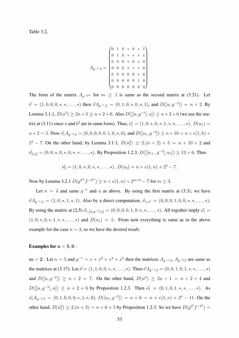
Table 3.2,
Ag−1,3 =
0 1 0 ∗ 0 ∗ 1
0 1 0 ∗ ∗ ∗ 1
0 0 0 ∗ 0 ∗ 0
0 0 0 1 ∗ ∗ 0
0 0 0 0 0 ∗ 0
0 0 0 0 0 1 0
0 0 0 0 0 0 0
.
The form of the matrix Ag−2m for m ≥ 1 is same as the second matrix at (3.21). Let
~ν = (1, 0, 0, 0, ∗, ∗, . . . , ∗) then ~νAg−1,3 = (0, 1, 0, ∗, 0, ∗, 1), and D([u, g−1]) = n + 2. By
Lemma 3.1.1, D(u2) ≥ 2n+ 5 ≥ n+ 2 + 6. Also D([[u, g−1], u]) ≥ n+ 2 + 6 (we use the ma-
trix at (3.11) since u and b2 are in same form). Thus, ~ν1 = (1, 0, ∗, 0, ∗, 1, ∗, ∗, . . . , ∗), D(u1) =
n+ 2 = 5. Now ~ν1Ag−2,5 = (0, 0, 0, 0, 0, 1, 0, ∗, 0), and D([u1, g−2]) ≥ n+ 10 = n+ e(1, k) +
24 − 7. On the other hand, by Lemma 3.1.1, D(u21) ≥ 2.(n + 2) + 5 = n + 10 + 2 and
~ν2,u21= (0, 0, ∗, 0, ∗, 0, ∗, ∗, . . . , ∗). By Proposition 1.2.3, D([[u,1 , g
−2], u1]) ≥ 13 + 6. Thus
~ν2 = (1, 0, ∗, 0, ∗, ∗, . . . , ∗), D(u2) = n+ e(1, n) + 24 − 7.
Now by Lemma 3.2.1 D(g2mf−2m) ≥ n+ e(1, n) + 2m+2 − 7 for m ≥ 3.
Let n = 4 and same g−1 and u as above. By using the first matrix at (3.3), we have
~νAg−1,4 = (1, 0, ∗, 1, ∗, 1). Also by a direct computation, ~ν1,u2 = (0, 0, 0, 1, 0, 0, ∗, ∗, . . . , ∗).
By using the matrix at (2.5) ~ν1,[[u,g−1],u] = (0, 0, 0, 0, 1, 0, ∗, ∗, . . . , ∗). All together imply ~ν1 =
(1, 0, ∗, 0, ∗, 1, ∗, ∗, . . . , ∗) and D(u1) = 5. From now everything is same as in the above
example for the case n = 3, so we have the desired result.
Examples for n = 5,6 :
m = 2 : Let n = 5 and g−1 = x + x2 + x4 + x5 then the matrices Ag−1,5, Ag−2,7 are same as
the matrices at (3.17). Let ~ν = (1, 1, 0, 0, ∗, ∗, . . . , ∗). Then ~νAg−1,5 = (0, 0, 1, 0, 1, ∗, ∗, . . . , ∗)
and D([u, g−1]) ≥ n + 2 = 7. On the other hand, D(u2) ≥ 2n + 1 = n + 2 + 4 and
D([[u, g−1], u]) ≥ n + 2 + 6 by Proposition 1.2.3. Then ~ν1 = (0, 1, 0, 1, ∗, ∗, . . . , ∗). As
~ν1Ag−2,7 = (0, 1, 0, 0, 0, ∗, 1, ∗, 0), D([u1, g−2]) = n + 6 = n + e(1, n) + 24 − 11. On the
other hand, D(u21) ≥ 2.(n + 3) = n + 6 + 5 by Proposition 1.2.3. So we have D(g22f−22) =
53
n + e(1, n) + 24 − 11. For n = 6, very similar argument as in previous cases works for the
same example of the case n = 5.
m ≥ 3 : Let n = 5 and g−1 = x + x2 + x3 + x4 + x7. Note that the matrices Ag−1,5, Ag−2m
for m ≥ 2 are same as the matrices at (3.18). Let ~ν = (1, 1, ∗, ∗, . . . , ∗). Then ~νAg−1,5 =
(0, 1, 1, ∗, 0, ∗, ∗, . . . , ∗) and so D([u, g−1]) = n + 2 = 7. On the other hand, D(u2) ≥ 2.n +
1 = n + 2 + 4 and D([[u, g−1], u]) ≥ n + 2 + 6 by Proposition 1.2.3. So we have ~ν1 =
(1, 1, ∗, 0, ∗, ∗, . . . , ∗) and D(u1) = n + 2 = 7. Now ~ν1Ag−2,7 = (0, 0, 0, 1, 0, ∗, 0, ∗, 0) so
D([u1, g−2]) = n + 8 = n + e(1, n) + 24 − 9. On the other hand, by a direct computation
D(u21) ≥ 2.(n + 2) + 1 = n + 8 + 2 and ~ν2,u21
= (0, 0, 1, 1, ∗, 0, ∗, ∗, . . . , ∗). So we have
~ν2 = (1, 0, ∗, 1, ∗, 0, ∗, ∗, . . . , ∗) and D(u2) = 13 = n + e(1, n) + 24 − 9 by Remark 3.2.1.
As ~ν2Ag−22 = (0, 0, 0, 0, 0, 0, 0, ∗, 0), we have D([u2, g−22 ]) ≥ n + e(1, n) + 25 − 9 + 2 ≥ 31
and ~ν3,[u2,g−22 ] = (0, 0, ∗, 0, ∗, ∗, . . . , ∗). By direct computation D(u22) = 29 and ~ν3,u22
=
(1, 0, ∗, 1, ∗, ∗, . . . , ∗). Hence, we have ~ν3 = (1, 0, ∗, 1, ∗, ∗, . . . , ∗) and D(u3) = 29 = n +
e(1, n) + 25− 9 by Remark 3.2.1. Let ~νm = (1, 0, ∗, 1, ∗, ∗, . . . , ∗) and D(um) = n+ e(1, n) +
2m+2 − 9 for m ≥ 3. Then (1, 0, ∗, 1, ∗, ∗, . . . , ∗)Ag−2m = (0, 0, 0, 0, 0, 0, 0, ∗, 0). It follows
that D([um, g−2m ]) ≥ n+ e(1, n) + 2m+3 − 9 + 2 and ~νm+1,[um,g−2m ] = (0, 0, ∗, 0, ∗, ∗, . . . , ∗).
On the other hand, it can be easily seen that D(u2m) = n + e(1, n) + 2m+3 − 9 and ~νm+1,u2m
=
(1, 0, ∗, 1, ∗, ∗, . . . , ∗). Hence, ~νm+1 = (1, 0, ∗, 1, ∗, ∗, . . . , ∗) and D(um+1) = n + e(1, n) +
2m+3−9 by Remark 3.2.1. Therefore, an inductive argument givesD(g2mf−2m) = D(u2m−1) =
n + e(1, n) + 2m+2 − 9 for m ≥ 3. For n = 6, because of a same argument as in the previous
cases, same example works to get the desired bound.
54
CHAPTER
4On random generation in the
Nottingham group
Being a pro-p group, the Nottingham group can be seen as a probabilistic space with respect to
the normalized Haar Measure. Recall that Q(G, k) is the probability that k random elements
generate an open subgroup of G for a profinite group G. A. Shalev [Sha00] pointed out that if
Q(G, k) = 1 then the lower rank of G is at most k. It is still not known whether the converse is
true or not. For p ≥ 3, the lower rank of N is 2, see [Cam00]. Following the relation between
the lower rank and the random generation, Shalev [Sha00] conjectured the following:
Conjecture 1. Is Q(N , 2) = 1?
The aim of this chapter is to investigate Conjecture 1 above. We will use a probabilistic
theorem which Szegedy [Sze05] used to prove that two random elements of the Nottingham
group generate a free subgroup. By invoking the following two propositions, we follow his
footsteps. The first is a corollary of a measure theoretical theorem from [Sak64, Chapter 4,
(15.7)Theorem].
Proposition 4.0.1. Let X be a metric space, and let Pn be a sequence of its partitions such that
Pn consists of Borel sets, Pn is a refinement of Pn−1, and the diameter of the sets in Pn is at
most dn, where dn tends to zero. Then for every Borel set E ⊂ X and finite Borel measure µ,
we have, for almost all x ∈ E
limn→inf
µ(E ∩Hn)
µ(Hn)= 1
where x ∈ Hn ⊂ Pn.
55
Let G be a pro-p group, Gi be a filtration of G and µ be the Haar measure induced by
the G-invariant metric d(x, y) = inf{|G : Gi|−1 : xy−1 ∈ Gi}. Recall that the balls in G
with respect to this metric are the cosets of Gi, and the diameter of such balls is |G : Gi|−1.
Applying the proposition above to G, we get the following
Proposition 4.0.2. Let E be a Borel set of G. Then for almost all x ∈ E,
limn→∞
µ(E ∩ xGn)
µ(xGn)= 1.
By using Proposition 4.0.2, the following conjecture implies Conjecture 1.
Conjecture 2. Let p ≥ 5. Then ∃ε > 0, ∀a, b ∈ N , ∃L0 ∈ N, ∀L1 ≥ L0 the conditional
probability P (〈au, bv〉 open|u, v ∈ NL1) ≥ ε.
To be more precise, take two random elements of N which generate a possibly non-open
subgroup. Then Conjecture 2 states that: changing the tales of those two elements, the new two
ones will generate an open subgroup with positive probability, depending only on p. To test
whether two elements generate an open subgroup we have the following result which follows
from the proof of a theorem in [Cam00, Theorem 7].
Theorem 4.0.3. Let p ≥ 5. Let a, b ∈ N with D(a) = q,D(b) = r. Then 〈a, b〉 is an open
subgroup of N whenever
(a) q 6≡ ∓r (mod p),
(b) q, r 6≡ 0 (mod p), and
(c) q and r are coprime.
From now on assume that p ≥ 5. The m-th Engel word (see Section 2.1) plays a significant
role in our approach. Related to this, we will state a lemma that will be one of our main tools.
The following definition is a generalization of a definition in [LGM02, Proposition 1.1.32].
Definition 4.0.4. Let G be a group, x1, x2, . . . , xk ∈ G, and n, i1, i2, . . . , ik ∈ N. Define
{x1, x2, . . . , xk}ni1,i2,...,ik to be the set of all formal basic commutators in {x1, x2, . . . , xk} of
weight at least n, and of weight at least ij in xj where ij < n for 1 ≤ j ≤ k.
56

Here we have another definition which can be seen as a generalized m-th Engel word.
Definition 4.0.5. Let x, y, z ∈ G and m ∈ N. We define the set
[x,{m} {y, z}] ={
[x,i1 y,j1 z, . . . ,ik y,jk z] |m = i1 + j1 + . . . ik+ jk, i1, j1, . . . , ik, jk, k ∈ N}.
Lemma 4.0.6. Let G be a group and a, b, u, v ∈ G. Then
[au,m bv] = [a,m b][u,m b]X
where X =∏
xt, the factors xt’s are different from [a,m b], [u,m b] and one of the following
types of commutators.
(T1) xt ∈ [X(i),{m−i} {b, v}], where 1 ≤ i ≤ m and we have one of the following:
• X(i) ∈ {a(i), u, v, a, b}i+11,0,0,0,0 involving at least one u or v and a(i) ∈ [a,{i} {b, v}],
• X(i) ∈ {u(i), u, v, a, b}i+11,0,1,0,0 where u(i) ∈ [u,{i} {b, v}].
(T2) xt ∈ [Y (i),{m−i} {b, v}] where Y (i) ∈ {u, v, a, b}2i+10,0,0,0 for some 1 ≤ i ≤ m such that the
sum of weights of u and v is at least 2 and the sum of the weights of b and v is at least
2i− 1.
Proof. Recall the following well known commutator identities, see [LGM02, Proposition
1.1.6]. Let x, y, z ∈ G. The conjugate of x by y is denoted by xy = y−1xy. Then
(i) [xy, z] = [x, z][x, z, y][y, z] = [x, z]y[y, z],
(ii) [x, yz] = [x, z][x, y][x, y, z] = [x, z][x, y]z,
(iii) xy = yx[x, y] = yxy.
By using the identities above, we can get the following generalization. Let x1, x2, · · · , xn, y ∈
G. Then
[x1x2 · · ·xn, y] = [x1, y]x2···xn [x2 · · ·xn, y]
= [x1, y]x2···xn [x2, y]x3···xn [x3 · · ·xn, y]
...
= [x1, y]x2···xn [x2, y]x3···xn · · · [xn, y].
57

On the other hand,
[xi, y]xi+1···xn = [xi, y][xi, y, xi+1 · · ·xn]
= [xi, y][xi, y, xi+2 · · ·xn][xi, y, xi+1]xi+2···xn
...
= [xi, y][xi, y, xn][xi, y, xn−1]xn [xi, y, xn−2]xn−1xn . . . [xi, y, xi+1]xi+2···xn .
Note that, by a similar technique above, any conjugate of [xi, y, xj] is a product of [xi, y, xj]
and commutators involving [xi, y, xj]. Hence, we have the following identity
(iv) The commutator [x1x2 · · ·xn, y] can be written as a product of [xi, y] for i = 1, 2, · · ·n
and product of commutators involving [xi, y, xj] for all 1 ≤ i < j ≤ n.
Back to the proof, we use induction on m ≥ 1. Let m = 1. By using the identities (i), (ii) and
(iii), we have
[au, bv] = [au, v][au, b][au, b, v]
= [a, v][a, v, u][u, v][a, b][a, b, u][u, b][[a, b][a, b, u][u, b], v
]Now we can bring forward [a, b] and [u, b] by using the commutator identity (iii). Then the rest,
but the last factor[[a, b][a, b, u][u, b], v
], is a product of [a, v], [a, v, u], [u, v], [a, b, u], which
belong to [X(i),{m−i} {b, v}] for i = 1,m = 1 that involves at least one u or v, and product
of commutators involving [a, b], [u, b] which are again in [X(i),{m−i} {b, v}] for i = 1,m = 1
that involves at least one u or v. Now by using identity (iv), the last factor can be written as a
product of commutators [a, b, v], [a, b, u, v], [u, b, v] and commutators involving [xi, v, xj] where
1 ≤ i < j ≤ 3 and x1 = [a, b], x2 = [a, b, u], x3 = [u, b]. So, they belong to [X(i),{m−i} {b, v}]
for i = 1,m = 1 that involves at least one u or v. Let m ≥ 1 and suppose that we have
[au,m b] = [a,m b][u,m b]X
where X is a product of commutators of the types in (T1) or (T2). By using the identity (ii),
58
we have
[au,m+1 b] =[[a,m b][u,m b]X, bv
]=[[a,m b][u,m b]X, v
][[a,m b][u,m b]X, b
][[a,m b][u,m b]X, b, v
].
Let c be either b or v. Now by using identity (iv), similar to the case when m = 1, the above
equality can be written as product of [[a,m b], v], [[u,m b], v], [[a,m b], b], [[u,m b], b], [X, v], [X, b],
[[a,m+1 b], v], [[u,m+1 b], v], [X, b, v] and commutators involving [xi, c, xj] for 1 ≤ i < j ≤ 3
where x1 = [a,m b], x2 = [u,m b], x3 = X . Now we can bring [a,m+1 b] and [u,m+1 , b] to
front by using the identity (iii) and the rest is product of commutators [[a,m b], v], [[u,m b], v],
[a,m+1 b, v], [u,m+1 b, v], [X, v], [X, b], [X, b, v], commutators involving [a,m+1 b] or [u,m+1 b]
and commutators involving [xi, c, xj] for 1 ≤ i < j ≤ 3, where x1 = [a,m b], x2 = [u,m b], x3 =
X . It can be easily seen that all, but [X, v], [X, b] and [X, b, v], are in [X(i),{m+1−i} {b, v}]
where i = m + 1. Now by induction, [X, c] = [∏
xt, c], where xt’s are commutators from
[X(i),{m−i} {b, v}] or [Y (i),{m−i} {b, v}] for some 1 ≤ i ≤ m. By using the identity (iv), we
can rewrite [X, b] as product of commutators [xt, c] and commutators involving [xt, c, xs] for
t < s. It can be directly seen that the commutators [xt, c]’s are from [X(i),{m+1−i} {b, v}]
or [Y (i),{m+1−i} {b, v}]. Since any xt is of weight at least m + 1 and the sum of weights
of b and v is at least m and involves at least one u or v, then the commutators [xt, c, xs] ∈
{u, v, a, b}2(m+1)+10,0,0,0 , the sum of weights of u and v is at least 2 and the sum of weights of b and
v is at least 2(m+ 1)− 1. Hence, they belong to [Y (i),{m+1−i} {b, v}] for i = m+ 1. It remains
only to consider [X, b, v]. Again, by using identity (iv), similar arguments which we applied
for [X, c] will give the desired.
§4.1 Random generation
Fix a, b ∈ N . Theorem 4.0.3 allows us to divide our investigation into four cases.
Case 0. Assume that 〈a, b〉 is open.
Case 1. Assume that all elements of 〈a, b〉 has p-divisible depth.
59

Case 2. Assume that every element in 〈a, b〉 has depth congruent to k0, −k0, or 0 modulo p for
some k0 6≡ 0 (mod p).
Case 3. Assume that the depths of all elements of 〈a, b〉 have a common divisor r 6≡ 0 (mod p),
where r > 1.
Case 0:
Assume that 〈a, b〉 is open. Then ∃L 6≡ 0, p − 1 (mod p) such that 〈a, b〉 ⊇ NL. Now,
∃w1, w2 ∈ 〈a, b〉 such that D(w1) = L 6= 0 and D(w2) = L + 1. Let L0 = L + 2 then
for any u, v ∈ NL0 , w′1 := w1(au, bv) ≡ w1(a, b) (mod xL0+1) and w′2 := w2(au, bv) ≡
w2(a, b) (mod xL0+1). Now, by Theorem 4.0.3, 〈w′1, w′2〉 is open with probability 1. Hence, for
all L1 ≥ L0, P (〈au, bv〉 open | u, v ∈ NL1) = 1.
Case 1:
Assume that all elements of 〈a, b〉 has p-divisible depth.
Proposition 4.1.1. Let L0 ≥ D(a), D(b). Then for all L1 ≥ L0 the probability that 〈au, bv〉,
for u, v ∈ NL1 , has an element whose depth is not divisible by p is ≥ 1p3
.
Proof. Pick n,m ∈ N such that:
1. n 6≡ 0 (mod p),
2. pm > n−D(a).
Consider the commutator [a,m b]. Since all elements in 〈a, b〉 has p-divisible depths, we have
D([a,m b]) ≥ D(a) +mD(b) + pm (4.1)
for all m ≥ 0. Indeed, note that D([a, b]) = D(a) + D(b) + d for some d ≥ 1. Since
D([a, b]), D(a), D(b) ≡ 0 (mod p), d ≡ 0 (mod p). On the other hand, we have d ≥ 1, so
d ≥ p. Hence, we have D([a, b]) ≥ D(a) + D(b) + p. Now applying an inductive proof will
give
D([a,m b]) ≥ D(a) +mD(b) +mp.
60

Let u, v ∈ NL0 such that D(u) = n and D(v) > n. Since D(u) 6≡ 0 (mod p), we have
D([u,m b]) = D(u) +mD(b).
Consider the commutator [au,m bv]. By Lemma 4.0.6, we have
[au,m bv] = [a,m b][u,m b]X,
where X is the product of commutators of the types in (T1) or (T2). It can be seen easily that
all factors of X has depth > D(u) + mD(b) = D([u,m b]). Indeed, let us first consider the
factors in X involving at least one u, but no v. Then the weight of such a factor is at least m+2
and the weight of b is at least m. Consequently, any such factor has depth strictly larger than
D(u) + mD(b). Now, consider the factors which do not involve any u, but at least one v. The
weight of such a factor is at least m + 1 and the sum of weights of b and v is at least m. It
follows that any such factor has depth strictly larger than D(u)+mD(b) as D(v) > n = D(u).
Since pm > n−D(a), we have
D([a,m b]) ≥ D(a) +mD(b) + pm > D(u) +mD(b) = D([u,m b]).
Thus, we have
D([au,m bv]) = D([u,m b]) = D(u) +mD(b) 6≡ 0 (mod p).
Since n 6≡ 0 (mod p), L0 ≤ D(u) ≤ L0 + 1. Also D(v) > D(u). So, for all L1 ≥ L0, the
probability that 〈au, bv〉, for u, v ∈ NL1 , has an element whose depth is not divisible by p is
≥ 1p3
.
We have the following corollary of Proposition 4.1.1.
Corollary 4.1.2. The probability that two randomly chosen elements from N generates a sub-
group where every element has depth divisible by p is zero.
By Corollary 4.1.2, we need to consider Case 0, Case 2 or Case 3 only.
61
Case 2 and Case 3:
The following observation is important for the investigations of Case 2 and Case 3.
Remark 4.1.1. Let w ∈ N with D(w) = k ≡ k0 (mod p) for 0 < k0 < p − 1. Let n ≥ k
be such that n 6≡ 2k − i (mod p) for any 0 ≤ i ≤ k0. So, n + 1 6≡ 2k − j (mod p) for
any 0 ≤ j < k0 and, therefore, e(k, n + 1) = k0 and e(k, n) = k0, see Definition 2.0.1. By
Lemma 2.1.4, we have Πp−1,n+1,k0 = 0 and Πp−1,n,k0 = 0. On the other hand, recall that we
obtain Πp−1,n+1,k0 by deleting the first column and row of Πp−1,n,k0+1. Recall also the definition
of the corresponding matrix Tn[λ] from Section 2.2. Now we have Tn[λ] = (λ) (note that λ is
the entry at the top right corner of Πp−1,n,k0+1 which may or may not be zero) for the element
w with respect to the integer n.
Based on the above, we make the following definition. Let w ∈ N with D(w) = k ≡
k0 (mod p) where 0 < k0 < p− 1. We define the following property for w:
(P∗) ∃n0 6≡ 0,−k0, 2k−i (mod p) for i = 0, 1, . . . , k0 such that Tn[λ] = (λ) 6= 0 ∀n ≡ n0 (mod p).
Remark 4.1.2. Let c, d ∈ N be such that D(c) ≥ D(d), D(c) ≡ D(d) ≡ k0 (mod p) for
some 0 < k0 ≤ p− 1 and the first k0 + 1 coefficients of c and d are same. Then they have the
same matrix Πp−1,n,e(k,n)+1 for any n ≥ D(c), D(d). So, for any D(u) ≥ n ≥ D(c), D(d), by
Lemma 2.1.6, we have
D(u(s(p−1))) ≥ n+ s(p− 1)D(d) + (s− 1)k0
where u(s(p−1)) ∈ [u,{s(p−1)} {c, d}].
Case 2
Assume that every element in 〈a, b〉 has depth congruent to k0, −k0, or 0 modulo p for some
0 < k0 < p− 1.
Proposition 4.1.3. Let L0 ≥ D(a), D(b). Suppose that D(a) > D(b) + k0 where D(b) = k ≡
k0 (mod p), k0 6≡ (p − 3)−1, 2(p − 3)−1, (p − 2)−1, 2(p − 2)−1, 2(p − 1) (mod p) and b has
62

property (P∗). Then for all L1 ≥ L0
P (〈au, bv〉 open | u, v ∈ NL1) ≥1
p2p2+9p
Before proving Proposition 4.1.3, we need the following result.
Lemma 4.1.4. Let c, d ∈ 〈a, b〉 be such that D(d) ≡ k0 (mod p) and k0 6≡ (p − 3)−1, 2(p −
3)−1, (p− 2)−1, 2(p− 2)−1, 2(p− 1) (mod p). Then
D([c,3m d]) ≥ D(c) + 3mD(d) + 3m
for all m ≥ 0.
Proof. We use induction on m ≥ 0. For m = 0 the claim is trivial. Now suppose that
D([c,3m d]) ≥ D(c)+3mD(d)+3m form > 0. We haveD([c,3m d]) ≡ k0,−k0, or 0 (mod p).
If D([c,3m+1 d]) ≡ k0 (mod p) then D([c,3m+2 d]) = D([c,3m+1 d]) + D(d) + l ≡
k0,−k0, 0 (mod p), where l ≥ 1. Then l ≡ −k0,−3k0,−2k0 (mod p). Since k0 6≡
(p−3)−1, 2(p−3)−1, (p−2)−1, 2(p−2)−1, 2(p−1), (p−1), 0 (mod p), we have l ≥ 3. Hence,
by induction hypothesis,D([c,3m+3 d]) ≥ D([c,3m+2 d])+D(d) ≥ D([c,3m+1 d])+2D(d)+l ≥
D(c) + (3m+ 3)D(d) + 3m+ 3.
If D([c,3m+1 d]) ≡ −k0 (mod p) then D([c,3m d]) ≡ k0 (mod p). Hence, D([c,3m+1 d]) ≥
D([c,3m d]) + D(d) + 3 because of our assumptions on k0 as in the previous case. Therefore,
D([c,3m+3 d]) ≥ D([c,3m+1 d]) + 2D(d) ≥ D([c,3m d]) + 3D(d) + l ≥ D(c) + (3m+ 3)D(d) +
3m+ 3 by induction.
If D([c,3m+1 d]) ≡ 0 (mod p) then D([c,3m+2 d]) = D([c,3m+1 d]) + D(d) ≡ k0 (mod p).
So, D([c,3m+3 d]) = D([c,3m+2 d]) + D(d) + 3 because of the same reason in the above cases.
Hence, by induction, D([c,3m+3 d]) ≥ D([c,3m+2 d]) +D(d) + 3 ≥ D([c,3m d]) + 3D(d) + 3 ≥
D(c) + (3m+ 3)D(d) + 3m+ 3.
Note that for m′ ≥ 1 the proof above shows that
D([a,m′ b]) ≥ D(a) +m′D(b) +m′ − l′,
63
where m′ ≡ l′ (mod 3) and 0 ≤ l′ ≤ 2. Also if we don’t have the conditions k0 6≡ (p −
3)−1, 2(p − 3)−1, (p − 2)−1, 2(p − 2)−1, (p − 1), 2(p − 1), (p − 1), 0 (mod p) then the proof
above ensures that for m ≥ 0 we still have
D([a,3m b]) ≥ D(a) + 3mD(b) +m.
Proof of Proposition 4.1.3. By assumption, b has property (P∗). So ∃n0 such that n0 6≡
0,−k0, 2k − i (mod p) for any 0 ≤ i ≤ k0 and Tn[λ] = (λ) 6= 0 ∀n ≡ n0 (mod p). Let
gcd(k, k0) = k1. Since p and k1 are coprime then ∃n ≡ n0 (mod p), n ≡ 1 (mod k1) and
L0 + k0 + 1 ≤ n < L0 + k0 + 1 + pk1 by using the Chinese Remainder Theorem. Note that
n ≡ 1 (mod k1)⇒ k1 | 1− n⇒ ∃ s′ such that s′k0 ≡ 1− n (mod k)
⇒ n+ s′k0 ≡ 1 (mod k)⇒ gcd(n+ s′k0, k) = 1⇒ gcd(n+ s′(p− 1)k + s′k0, k) = 1
⇒ gcd(n+ s(p− 1)k + sk0, k) = 1 ∀s ≡ s′ (mod k).
Now pick s ≡ s′ (mod k) such that n−D(a) < s(p− 1)− sk0− l where s(p− 1) ≡ l (mod 3)
and 0 ≤ l ≤ 2. Let u, v ∈ N be such that D(u) = n, D(v) > n+ 5k0 + p, D(v) ≡ k0 (mod p)
and first k0 + 1 coefficients of v are same as first k0 + 1 coefficients of b. Since b has property
(P∗), D([u,s(p−1) b]) = n+ s(p− 1)k + sk0 by the proof of Theorem 2.0.3 in Chapter 2. Now
consider the commutator [au,s(p−1) bv]. Set m = s(p− 1). By Lemma 4.0.6 we have
[au,m bv] = [a,m b][u,m b]X,
where X is the product of commutators of type (T1), (T2). Let X ′ be the factor which has the
minimum depth. NowX ′ is from [X(i),{m−i} {b, v}], or [Y (i),{m−i} {b, v}] for some 1 ≤ i ≤ m.
Recall that we have one of the following
• X(i) ∈ {a(i), u, v, a, b}i+11,0,0,0 which involves at least one u or v and a(i) ∈ [a,{i} {b, v}],
• X(i) ∈ {u(i), u, v, a, b}i+11,0,1,0 where u(i) ∈ [u,{i} {b, v}].
Recall also, Y (i) ∈ {u, v, a, b}2i+10,0,0,0 is such that the sum of weights of u and v is at least 2 and
the sum of weights of b and v is at least 2i − 1. Suppose that X ′ is in [X(i),{m−i} {b, v}] for
some 1 ≤ i ≤ m and X(i) ∈ {a(i), u, v, a, b}i+1,1,0,0,0 which involves at least one u or v and
64
a(i) ∈ [a,{i} {b, v}]. Suppose that D(X(i)) involves at least one v, but does not involve any u.
Set m = s(p − 1). Now we have either a(i) ∈ [a,j−1 b, v,{i−j} {b, v}] for some 1 ≤ j ≤ i or
a(i) = [a,i b]. Suppose that we have the former. Let j−1 = s1(p−1)+ i1, i−j = s2(p−1)+ i2
and m − i = s3(p − 1) + i3. Then s ≥ s1 + s2 + s3 ≥ s − 2. Now, by Remark 4.1.2 and
Lemma 4.1.4,
D(X(i)) ≥ D([a,j−1 b]) +D(v) + (i− j)D(b) + (s2 − 1)k0
≥ D(a) + (j − 1)D(b) + j − 3 +D(v) + (i− j)D(b) + (s2 − 1)k0
≥ D(a) + (i− 1)D(b) +D(v) + j − 3 + (s2 − 1)k0.
Then
D(X) ≥ D(X ′) ≥ D(a) + (j − 1)D(b) + j − 3 +D(v) + (i− j)D(b)
+(s2 − 1)k0 + (m− i)D(b) + (s3 − 1)k0
> n+mD(b) + (s1 + s2 + s3 − 2 + 5)k0
≥ n+ s(p− 1)k + sk0
by Remark 4.1.2, Lemma 4.1.4, D(a) > D(b) + k0, D(v) > n+ 5k0 + p and k0 < p− 1. Now
suppose that we have the latter or X(i) involves at least one u, but does not involve any v. Then
in both cases we have a(i) = [a,i b] and X(i) involves at least one u or v. So
D(X(i)) ≥ D(a) + iD(b) + i− 2 +D(u)
by using Lemma 4.1.4. Let i = t1(p−1)+ l1 and m− i = t2(p−1)+ l2 for some l1, l2 < p−1.
Then s ≥ t1 + t2 ≥ s − 1. Now similar to above, by Remark 4.1.2, D(a) > D(b) + k0 and
k0 < p− 1, we have
D(X) ≥ D(a) + iD(b) + i− 2 +D(u) + (m− i)D(b) + (t2 − 1)k0
> n+mD(b) + (t0 + t2 + 1)k0 ≥ n+ s(p− 1)k + sk0.
Now for the other possible forms of X ′, by using very similar techniques above, we can show
that D(X ′) > n + s(p − 1)k + sk0 and, so, D(X) > n + s(p − 1)k + sk0 = D([u,s(p−1) b]).
65

Thus
[au,m bv] ≡ [a,m b][u,m b] (mod xD([u,mb])+2).
Recall that we picked s such that n−D(a) > s(p− 1)− sk0 − l. Then by Lemma 4.1.4,
D([a,s(p−1) b]) ≥ D(a) + s(p− 1)D(b) + s(p− 1)− l
> n+ s(p− 1)k + sk0 = D([u,s(p−1) b]).
Finally,
D([au,s(p−1) bv]) = D([u,s(p−1) b]) = n+ s(p− 1)k + sk0.
Now D(bv) = k and D([au,s (p − 1)bv]) = n + s(p − 1)k + sk0 satisfy the conditions of
Theorem 4.0.3. It follows that the subgroup 〈[au,s(p−1) bv], bv〉 is open with probability ≥1
pp2+p2+p+5k0+p+p+k0+1
≥ 1
p2p2+9pasL0 ≤ D(u) ≤ L0+k0+pk1+1 ≤ L0+p2,D(v) > n+5k0+p,
D(v) ≡ k0 (mod p) and its first k0 + 1 coefficients are same as the first k0 + 1 coefficients of b.
Hence, 〈au, bv〉 is open with probability ≥ 1
p2p2+9p.
Case 3:
Assume that the depths of all elements of 〈a, b〉 have a common divisor r 6≡ 0 (mod p) where
r > 1 and there exist elements whose depths are not divisible by p (to distinguish Case 1 and
Case 3 ).
Proposition 4.1.5. Let L0 ≥ D(a), D(b). Suppose that D(a) > D(b) + k0 where D(b) = k ≡
k0 (mod p), 0 < k0 < p− 1, k0 < r and b has the property (P∗). Then, for all L1 ≥ L0,
P (〈au, bv〉 open | u, v ∈ NL1) ≥1
2p2 + 9p.
To prove the above proposition we need the following lemma.
Lemma 4.1.6. Let c, d ∈ 〈a, b〉 be such that D(d) 6≡ 0 (mod p). Then
D([c,s(p−1)+1 d]) ≥ D(c) + (s(p− 1) + 1)D(d) + sr
for all s ≥ 0.
66
Proof. We will prove by induction on s ≥ 0. For s = 0, we have the claim. Now suppose that
we have
D([c,s(p−1)+1 d]) ≥ D(c) + (s(p− 1) + 1)D(d) + sr
for s ≥ 0. Note that there exists 1 ≤ i ≤ p − 1 such that D([c,s(p−1)+i d]) ≡
D(d), or 2D(d) (mod p). If D([c,s(p−1)+i d]) ≡ 2D(d) (mod p) then D([c,s(p−1)+i−1 d]) ≡
D(d) (mod p). It follows that
D([c,s(p−1)+i d]) ≥ D([c,s(p−1)+i−1 d]) +D(d) + pr
⇒ D([c,(s+1)(p−1)+1 d]) ≥ D(c) + ((s+ 1)(p− 1) + 1)D(d) + (s+ 1)r
by induction. Now if D([c,s(p−1)+i d]) ≡ D(d) (mod p) then
D([c,s(p−1)+i+1 d]) ≥ D([c,s(p−1)+i d]) +D(d) + r
⇒ D([c,(s+1)(p−1)+1 d]) ≥ D(c) + ((s+ 1)(p− 1) + 1)D(d) + (s+ 1)r
by induction.
Let us turn to the proof of Proposition 4.1.5.
Proof of Proposition 4.1.5. The proof is very similar to the proof of Proposition 4.1.3. Indeed,
since b has the property (P∗), ∃n0 such that n0 6≡ 2k−i for any 0 ≤ i ≤ k0 and Tn(λ) = (λ) 6=
0 ∀n ≡ n0 (mod p). Let k1 = gcd(k, k0). Now, by the Chinese Remainder Theorem, we can
pick n such that n ≡ n0 (mod p), n ≡ 1 (mod k1), and L0 + k0 + 1 ≤ n < L0 + k0 + pk1 + 1.
Also by using a very similar argument to the proof of Proposition 4.1.3, we can pick s such that
gcd(n+ s(p− 1)k + sk0, k) = 1 and n−D(a) < s(r− k0)− r (note that we could guarantee
the second condition on s because k0 < r). Then, by applying the same argument as in the
proof of Proposition 4.1.3, we get
[au,s(p−1) bv] ≡ [a,s(p−1) b][u,s(p−1) b] (mod x[u,s(p−1)b]+2),
where u, v ∈ NL0 such that D(u) = n, D(v) > n + 5k0 + p, D(v) ≡ k0 (mod p) and the first
67
k0 + 1 coefficients of b and v are same. On the other hand, by Lemma 4.1.6,
D([a,s(p−1) b]) ≥ D(a) + s(p− 1)D(b) + (s− 1)r
since s(p− 1) = (s− 1)(p− 1) + 1 + p− 2. Then
D([a,s(p−1) b]) > D([u,s(p−1) b]) = D(u) + s(p− 1)D(b) + sk0,
since n − D(a) < s(r − k0) − r. Hence, we have the commutator [au,s(p−1) bv] whose depth
is as desired. So, [au,s(p−1) bv] and bv generate an open subgroup with probability ≥ 1
p2p2+9pby
Theorem 4.0.3 . Therefore, 〈au, bv〉 is open with probability ≥ 1
p2p2+9p.
§4.2 Discussions
Here, we argue some possible developments of some techniques that seem promising for a
complete confirmation of Shalev’s conjecture. It is worth to mention that we have tried to
accomplish these ideas, but we could not be successful for the time being. This is due to
several difficulties that we will also discuss below.
First idea: Suppose that neither a nor b has the property (P∗). We argue a possible extension
of our work for the case when there exists a word in a, b having property (P∗). So, suppose
that there exists w2(a, b) ∈ 〈a, b〉 that has the property (P∗). Let w1(a, b) ∈ 〈a, b〉 be such that
D(w1) ≥ D(w2) and L0 ≥ D(w1), D(w2). Then for any u, v ∈ NL0+1, we have
w1(au, bv) ≡ w1(a, b)u for some u ∈ NL0+1
w2(au, bv) ≡ w2(a, b)v for some v ∈ NL0+1
Now, the idea is to apply the arguments used in the previous section for the commutator
[w1u,s(p−1)w2v]. For that, we need to guarantee that these new u and v satisfy the desired
properties. Here is the difficulty. For instance, it is not easy to guarantee that D(u) is co-prime
to D(w2) and, D(v) is congruent to D(w2) and both of them share the first k0 + 1 coefficients
(here D(w2) ≡ k0 (mod p) and 0 < k0 < p − 1). Although, we are free only to prescribe the
first few coefficients of u and v, we do not know yet how to choose these first few coefficients
68
in a way that u and v have the desired properties. A careful analysis on how the coefficients of
u and v affect the new word w(au, bv) might help us to overcome the difficulties above. But
certainly, this is intricate.
To accomplish this idea and to give a complete answer of Shalev’s conjecture, we need also
to consider the following question. Why would there exist a w(a, b) ∈ 〈a, b〉 with property
(P∗)?
Second idea: This idea depends on the role of the growth rate of certain Engel words. First,
we introduce the concept of the speed of an element, which is interesting in its own. From now
on, k0 denotes the smallest non-negative residue (modulo p) of the depth of a given element b.
Definition 4.2.1. Let a, b ∈ N . Define
s(a, b) = lim infm→∞
D([a,m b])−D(a)−mD(b)
m
the relative speed of b with respect to a. Now define
s(b) = mina∈N
s(a, b)
the speed of b.
Now, we consider the relative speed of b in a subgroup of N that contains b. Let H ≤ N
be such that b ∈ H . Then the relative speed of b in H is given by
sH(b) = mina∈H
s(a, b).
Lemma 2.1.6 is essentially saying that s(b) ≥ k0p−1
for any b ∈ N . Moreover, in Lemma 2.2.2
and Lemma 2.2.3, we could construct b such that s(b) = k0p−1
. In fact, we can tell more. Recall
the constant e′(k, n) (see Section 2.2). By Corollary 2.1.5 if the top right hand e′(k, n) + 1 ×
e′(k, n) + 1 block of Πp−1,n,e(k,n)+e′(k,n)+1 (for k+k0 +pt < n < k+p(t+ 1) where k = D(b)
and t is some nonnegative integer) is a non-nilpotent matrix then s(b) = k0p−1
. So, our condition
on b, having the property (P∗), in Case 2 and Case 3 implies that s(b) = k0p−1
.
Now let us compare sH(b) with s(b), where H is a non-open subgroup that contains b. For
example, in Case 1, s〈a,b〉(b) ≥ p while s(b) = 0. In Case 2 and Case 3, s〈a,b〉(b) ≥ 1 and rp−1
,
69

respectively, while s(b) = k0p−1
. As we see in all cases s(b) is small compared with s〈a,b〉(b). In
fact, s(b) is the minimum possible. However, there might be many elements whose speeds are
strictly larger than k0p−1
. For example, if b ≡ x+ xk+1 (mod xk+2k0+2), where k0 6≡ 0 (mod p),
then the associated matrix mentioned above is nilpotent. So, very possibly, s(b) > k0p−1
. Here,
we may try to find the exact speed of b by extending the matrix at (2.5) more carefully. But, even
if we find the exact speed, we may face another problem in comparing s(b) with s〈a,b〉(b). To
overcome this problem, we may try to determine the best possible minimum relative speed of an
element, whose depth is not divisible by p, in a non-open subgroup. Essentially, Lemma 4.1.4
and Lemma 4.1.6 imply that the relative speed of an element in a non-open subgroup must be
≥ 2p−1
if p ≥ 7 (remember that without the conditions on k0 in the statement of Lemma 4.1.4,
we have s〈a,b〉(d) ≥ 13). In fact, this gives us the following proposition.
Proposition 4.2.2. Let a, b ∈ N . If there exists c ∈ 〈a, b〉 such that D(c) 6≡ 0 (mod p) and
s〈a,b〉(c) <2p−1
then 〈a, b〉 is open.
Here, we have to mention that even if we can overcome the above problems, the real chal-
lenge is how to use this to confirm the conjecture under the question. In more details, even if
we have s(b) < s〈a,b〉(b), can we find a u ∈ N such that s(u, b) = s(b) with D([u,m b]) and
D(b) satisfying the criterion given in Theorem 4.0.3?
We also note that the concepts of speed and relative speed are interesting in their own,
and worth investigating. We are hoping that a future work on this topic would give better
understanding and would result in solving Shalev’s conjecture completely.
70


BIBLIOGRAPHY
[AH16] T. Aslan and P. Hegedus. Maximal deviation of large powers in the Nottingham
group. Submitted, 2016.
[Asl16] T. Aslan. The distance of large powers in the Nottingham group for p = 2.
Submitted, 2016.
[BL04] Y. Barnea and M. Larsen. Random generation in semisimple algebraic groups
over local fields. J. Algebra, 271(1):1–10, 2004.
[Cam96] R. Camina. Subgroups of the Nottingham Group. PhD thesis, University of Lon-
don, UK, 1996.
[Cam97] R. Camina. Subgroups of the Nottingham group. J. Algebra, 196(1):101–113,
1997.
[Cam00] R. D. Camina. The Nottingham group. In M. du Sautoy, D. Segal, and A. Shalev,
editors, New Horizons in Pro-p Groups, volume 184 of Progress in Mathematics,
pages 205–221. Birkhauser, Basel, 2000.
[DdSMS99] J. D. Dixon, M.P.F. du Sautoy, A. Mann, and D. Segal. Analytic pro-p Groups,
volume 61 of Cambridge Studies in Advanced Mathematics. Cambridge Univer-
sity Press, 1999.
[Dix69] J. D. Dixon. The probability of generating the symmetric group. Math. Z.,
110:199–205, 1969.
[dSSS00] M. du Sautoy, D. Segal, and A. Shalev. New Horizons in Pro-p Groups, volume
184 of Progress in Mathematics. Birkhauser, Basel, 2000.
73
[Ers04] M. Ershov. New just-infinite pro-p groups of finite width and subgroups of the
Nottingham group. J. Algebra, 275(1):419–449, 2004.
[Ers05] M. Ershov. The Nottingham group is finitely presented. J. London Math. Soc.,
71(2):362–378, 2005.
[FJ86] M. D. Fried and M. Jarden. Field Arithmetic. Springer, Berlin; Heidelberg, 1986.
[Heg01] P. Hegedus. The Nottingham group for p = 2. J. Algebra, 246(1):55–69, 2001.
[Joh88] D. L. Johnson. The group of formal power series under substitution. J. Austral.
Math. Soc., 45(3):296–302, 1988.
[Kea05] K. Keating. How close are p-th powers in the Nottingham group? J. Algebra,
287(2):294–309, 2005.
[KL90] W. M. Kantor and A. Lubotzky. The probability of generating a finite classical
group. Geom. Dedicata, 36(1):67–87, 1990.
[KLGP97] G. Klaas, C. R. Leedham-Green, and W. Plesken. Linear Pro-p-Groups of Finite
Width, volume 1674 of Lecture Notes in Mathematics. Springer-Verlag Berlin
Heidelberg, 1997.
[LGM02] C. R. Leedham-Green and S. McKay. The structure of groups of prime power
order. Oxford University Press, Oxford, 2002.
[MA96] M.W.Liebeck and A.Shalev. Simple groups, probabilistic methods, and a conjec-
ture of kantor and lubotzky. J. Algebra, 184(1):31–57, 1996.
[Man96] A. Mann. Positively finitely generated groups. Forum Math., 8:429–459, 1996.
[MS96] A. Mann and A. Shalev. Simple groups, maximal subgroups, and probabilistic
aspects of profinite groups. Israel J. Math., 96(B):449–468, 1996.
[Net82] E. Netto. Substitutionentheorie and ihre Anwendungen auf die Algebra. Teubner,
Leipzig, 1882. English transl. 1892, second ed., Chelsea, New York, 1964.
74
[Pin98] R. Pink. Compact subgroups of linear algebraic groups. J. Algebra, 206(2):438–
504, 1998.
[Sak64] S. Saks. Theory of the integral. Dover Publications, Inc., New York, 1964.
[Sha99] A. Shalev. Probabilistic group theory. In C. M. Campbell, E. F. Robertson,
N. Ruskuc, and G. C. Smith, editors, Groups St. Andrews 1997 in Bath, Lon-
don Math. Soc. Lecture Note Series 261, pages 648–678. Cambridge University
Press, Cambridge, 1999.
[Sha00] A. Shalev. Lie methods in the theory of pro-p groups. In M. du Sautoy, D. Segal,
and A. Shalev, editors, New Horizons in Pro-p Groups, pages 1–54. Birkhauser,
Basel, 2000.
[Sze05] B. Szegedy. Almost all finitely generated subgroups of the Nottingham group are
free. Bull. London Math. Soc., 37(1):75–79, 2005.
[Yor90a] I. O. York. The exponent of certain p-groups. Proc. Edinburg Math. Soc.,
33(3):483–490, 1990.
[Yor90b] I. O. York. The group of formal power series under substitution. PhD thesis,
Nottingham University, UK, 1990.
75


Recommended