On the Aggregation of Total Factor Productivity Measures*
by
Franklin A. Soriano** School of Economics
University of Queensland Brisbane, QLD, 4072, Australia
Email:[email protected]
D.S. Prasada Rao and Tim Coelli Centre for Efficiency and Productivity Analysis
School of Economics University of Queensland
Brisbane, QLD, 4072, Australia Web: http://www.uq.edu.au/economics/cepa.htm
December 2003
_____________________________________________________________________ *This preliminary paper is written for the 2003 Economic Measurement Group Workshop, University of New
South Wales, NSW, Australia, 11-12 December 2003.
**The author acknowledges the Australian Research Council -Strategic Partnership for Industry Research and
Training (SPIRT) Scholarship Grant for funding his Ph D candidature at UQ School of Economics. He is also
indebted to the Australian Bureau of Statistics (ABS) for the financial, technical and data support for the project.
2
1. Background
In recent years, policy makers and economic analysts have exhibited growing interest
in the measurement of productivity. Some analysts are interested mainly in measuring
the performances at firm, plant or division levels while others are concerned in the
productivity growth of particular industries, sectors or the whole economy. A great
deal of concern among economists and statistician over the last years is the relation
between aggregate and firm level productivity measures. This includes: the extent to
which these unit level productivity growth measures can be consistently aggregated;
the validity of the underlying assumptions in aggregate analyses; the search for a
possible aggregation approach with nice properties; and, the choice of the weights.
Over the decades, a large number of published studies have investigated aggregation
of efficiency measures. Most common are the measurement of technical efficiency,
allocative inefficiency as well as overall economic efficiency. A very important issue
on the measurement of productive efficiency initially raised by Farrell (1957) is on
the computation of an industry performance measure consistent with the aggregates of
individual firm performance measures. This has motivated some researchers to
investigate further. Several issues on aggregation have been discussed and examined
by: Li and Ng (1995); Blackorby and Russel (1999); Fox (1999); Bogetoft (1999);
Briec, Dervaux and Leleu (2002) and Fare and Grosskopf (2002).
A more recent paper of Fare and Zelenyuk (2003) demonstrated a new approach in
aggregating Farrell efficiency measures and discover conditions under which firm
level efficiencies can be aggregated to obtain an industry level efficiency. This
industry overall revenue efficiency measure is an output value (observed)-weighted
average of the firms’ revenue efficiencies. Moreover, Fare and Zelenyuk (2003) made
use of the Li and Ng (1995) results to decompose the said industry overall efficiency
measure into aggregate allocative and aggregate technical efficiency measures. In
addition, an industry technical efficiency measure is also introduced which is a multi-
output generalisation of the Farrell (1957) measure of structural efficiency of an
industry.
3
Fare and Zelenyuk (2003) stated: “To define the industry revenue function and obtain
an aggregation theorem, it is crucial that all firms face the same output price vector.”
In the real world, firms belonging to a certain industry producing the same commodity
may have different output prices. Moreover, they may also face different prices for
their inputs. So, it is useful to examine the effects of relaxing the output price
condition (i.e. same for all firms) on their aggregation and decomposition procedures.
Reallocation of industry resources among firms also plays an important role in any
aggregation exercise. Farrell (1957) in his seminal paper disclosed that “two firms
which, taken individually, are technically efficient, are not perfectly technically
efficient when taken together. In general, this implies that the industry outputs may
not be on the industry production frontier, even if each firm of the industry is
efficiently operating on its production frontier. This brought Fare et al (1992) to
extend the Johansen approach and formulate an industry production model that allows
some input(s) to be firm specific (not reallocatable) and some to be allocatable across
firms in an industry performance measurement. Their finding is that when all inputs
are reallocatable, industry is at least as large as when only some inputs are, and that
when no input is reallocatable, industry output is smallest. Li and Ng (1995) in their
measurement of productive efficiency of a group of firms shows that shadow revenue
of a group of firms can indeed be further increased through reallocation of inputs
among firms. Labour, energy, materials and other services inputs in an industry can be
reallocated across firms while the possibility of reallocating capital resources is very
little or none at all in the short-run.
To be able to effectively reallocate resources across firms, one has to know industry
technology. One can derive industry technology by summing individual firm
technologies, just like what Fare and Zelenyuk (2003) adopted in their study.
Moreover, they assumed that each firms faces different technology. Though summing
of individual firm’s technology to define the industry technology make sense, it make
more sense to talk about industry and firms efficiency measures if we imposed the
same technology to all firms in the industry.
In this paper, we first aim to examine and evaluate the behaviour of all the efficiency
measures developed by Fare and Zelenyuk (2003) when we relax the assumptions
4
that: (a) firms face the same price; and, (b) no reallocation of resources among firms.
In fact, the paper numerically examines the behaviour of the aggregate efficiency
measures that allow some inputs (capital and others) to be firm specific (not
reallocatable) and labour, energy, materials or other services inputs to be allocatable
across firms in an industry. In addition, the paper also looks at the efficiency measures
when same technology is imposed for each individual firm.
With a good result in the first objective, this paper will then attempt to investigate the
dynamic behaviour of TFP index with the aim of defining an industry Malmquist TFP
index. The present paper will first consider the output oriented Malmquist TFP. If
successful, a parallel application will be done using the input-oriented Malmquist TFP
index later.
This paper was motivated by a desire to measure industry TFP change from the firm
level TFPs. Using the traditional TFP index methods, Fox (2002) aggregation method,
and Balk (2001) method, the third objective of the paper is to empirically examine the
different industry level TFP measures. Fox (2002) provides alternative aggregation
method which satisfies monotonicity property while Balk (2001) measures
productivity level and productivity change based on real profitability. With the
availability of extensive micro data bases for market industry which provide input,
output and price data at the firm level, we assess the sensitivity of the aggregate
productivity results. A very important issue on aggregation which the paper looks at is
on the calculation of the relative size of each firm (weights) used in each of the
aggregation procedures. These include methods based on revenue and cost shares. A
part of this study is the investigation of the use of shadow shares, an objective that
will be pursued in future research.
This paper is organised into sections. In Section 2 we show how the Farrell output
oriented efficiency indexes could be aggregated when firms face different output
prices. We also investigate the effect of reallocation of allocatable inputs across firms
in the industry in the aggregation process. A numerical illustration ends the section
making use of the Australian Bureau of Statistics (ABS) microdata from the 1998
ABS Confidentialised Unit Record File (CURF). In Section 3, we briefly review the
different firm and industry productivity measures and start to define the industry

5
Malmquist TFP index in Section 4. We also present selected results from the
empirical applications of the aggregation methods using the Australian Bureau of
Statistics (ABS) microdata from the 1994-95 to 1997-98 ABS Confidentialised Unit
Record File (CURF). We consider 100 firms from the Clothing, Textile, Footwear and
Leather manufacturing industry (ANZSIC Code 22). Finally, some concluding
remarks are presented in Section 5.
2. Aggregating the Farrell output orientated efficiency indexes when firm faces different output prices
In this section, we re-examine the Fare and Zelenyuk (2003) methods. We relax the
assumption that firms face the same output price and show how industry output
(revenue) efficiency can be derived from the member firms’ output efficiency. At the
latter part, we relate this to the industry output oriented technical and allocative
efficiency measures. The section will take into account the output (or revenue)
oriented measures of Farrell (1957) efficiency framework. A parallel investigation
was also executed and applied to the input oriented case but for the present paper it
will not be presented and discussed.
2.1 Technology sets Consider the case of an industry with K firms, k=1, 2, 3,…, K, K>1. Each kth firm has
an input vector NkNk
k xxx +ℜ∈= ),...,( 1 , N inputs, and output
vector MkMk
k yyy +ℜ∈= ),...,( 1 , M outputs.
Note that as a notation for the present paper, vectors without superscripts (but
sometimes with primes) will be utilised as variables. Vectors with bars will represent
observations, thus for instance ),( kk yx denotes the input and output quantities of firm
k.
6
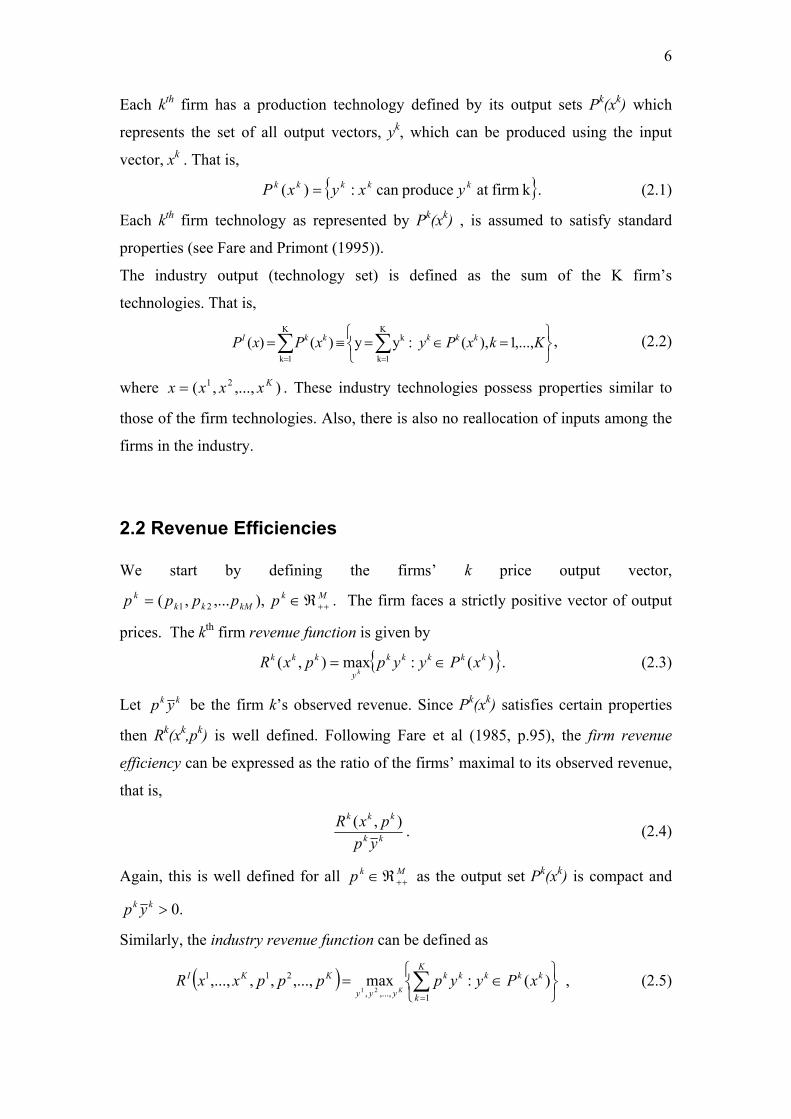
Each kth firm has a production technology defined by its output sets Pk(xk) which
represents the set of all output vectors, yk, which can be produced using the input
vector, xk . That is,
{ }k firmat producecan :)( kkkkk yxyxP = . (2.1)
Each kth firm technology as represented by Pk(xk) , is assumed to satisfy standard
properties (see Fare and Primont (1995)).
The industry output (technology set) is defined as the sum of the K firm’s
technologies. That is,
∑ ∑= =
=∈=≡=K
1k
K
1k
k ,...,1),( :yy)()( KkxPyxPxP kkkkkI , (2.2)
where ),...,,( 21 Kxxxx = . These industry technologies possess properties similar to
those of the firm technologies. Also, there is also no reallocation of inputs among the
firms in the industry.
2.2 Revenue Efficiencies We start by defining the firms’ k price output vector,
),,...,( 21 kMkkk pppp = Mkp ++ℜ∈ . The firm faces a strictly positive vector of output
prices. The kth firm revenue function is given by
{ })(:max),( kkkkk
y
kkk xPyyppxRk
∈= . (2.3)
Let kk yp be the firm k’s observed revenue. Since Pk(xk) satisfies certain properties
then Rk(xk,pk) is well defined. Following Fare et al (1985, p.95), the firm revenue
efficiency can be expressed as the ratio of the firms’ maximal to its observed revenue,
that is,
kk
kkk
yppxR ),( . (2.4)
Again, this is well defined for all Mkp ++ℜ∈ as the output set Pk(xk) is compact and
.0>kk yp
Similarly, the industry revenue function can be defined as
( )
∈= ∑=
)(:max,...,,,,...,1,...,,
21121
kkkK
k
kk
yyy
KKI xPyyppppxxRK
, (2.5)

7
and the industry revenue efficiency as
( )∑=
K
k
kk
KKI
yp
pppxxR
1
211 ,...,,,,..., . (2.6)
Note that ( )KKI pppxxR ,...,,,,..., 211 is well defined as the industry faces strictly
positive vector of output prices given by p=(p1,p2,…,pK) M++ℜ∈ and seek to maximize
the revenue .,...,2,1,)(,1
KkxPyyp kkkK
k
kk =∈∑=
Note that .01
>∑=
K
k
kk yp
Using the revenue version of the Koopmans’ Theorem (Fare and Grosskopf, 2002,
p.106) which states that “the industry maximal revenue is the sum of the firms’
maximal revenues,” (2.5) is then equal to the sum of (2.3), that is,
( ) ∑=
++ℜ∈=K
k
MkkkkKKI ppxRppxxR1
11 , ),(,...,,,..., . (2.7)
The proof is straightforward.
Thus, relating (2.4) and (2.6) combined with (2.7), we define the industry overall
output (or revenue) efficiency as the share-weighted average of the firms’ revenue
efficiencies. This is given by
( ) kK
kkk
kkk
K
k
kk
KKIIO os
yppxR
yp
ppxxRRE ×== ∑∑ =
=
1
1
11 ),(,...,,,..., , (2.8)
where ∑=
= K
k
kk
kkk
yp
ypos
1
is the kth firm’s observed revenue share. Note that 11
=∑=
K
k
kos
and .10 ≤< IORE
Also, note that (2.4) and (2.6) by definitions are bigger than or equal to one, hence
(2.8) satisfies the Aggregation Indication Axiom (AI) of Blackorby and Russel
(1999), which states that “the industry is considered to be efficient if and only if each
of its firms is efficient.” Clearly,
( ) k. allfor ,1),( ifonly and if 1,,...,
1
1
==
∑=
kk
kk
K
k
kk
KI
yppxR
yp
pxxR

8
2.3 Distance functions
We now focus at the distance functions for our firm technologies defined in Section
2.1. Firstly, we define an output-oriented distance function on the output set Pk(xk) ,
k=1,2,…,K , as
( ){ }.)(,0:inf),( kkkkkkkkkO xPyyxD ∈>= δδδ (2.9)
Since the outputs are disposable, we then have
1),()( ≤∈ kkkO
kkk yxDifonlyandifxPy , (2.10)
which means that the distance function, ),( kkkO yxD , will take a value less than or
equal to one if the output vector, yk, is an element of the feasible production set,
Pk(xk). It will also be increasing in xk and linearly homogeneous in yk.
Following Fare and Zelenyuk (2003), we define an output-oriented distance function
for the industry technology as
( ){ }
∑∑
∑∑
==
==
∈≤
=>∈=
∈
>=
K
1k1
1
11
1
).( as 1),,...,(
,...,2,10),(: inf max
)(,0:inf),,...,(
xPyyxxD
KkallforxPy
xPyyxxD
IkK
k
kKIO
kkkkkk
IK
k
kK
k
kKIO
δδδ
δδδ
δ
(2.11)
2.4 Technical Efficiencies
Following Fare et al (1985), the Farrell output-oriented technical efficiency for the kth
firm is given by
1 ),,( ≤= kO
kkkO
kO TEyxDTE . (2.12)
If 1=kOTE , then firm k is said to be output technically efficient. This technical
efficiency measure satisfies the following desirable properties (see Fare et al (1985)).
The industry output-oriented Farrell technical efficiency measure is given by

9
.1,),,...,,(1
21 ≤= ∑=
IO
K
k
kKIO
IO TEyxxxDTE (2.13)
The right hand side of the equation is obtained using (2.11). Equation (2.13) also
satisfies the desirable properties and they are independent of the output prices.
Following Fare and Zelenyuk (2003), we can define a share-weighted output oriented
industry technical efficiency measure using industry member’s individual technical
efficiencies (2.12) as
( ) 1ˆ,,11
≤×=×= ∑∑==
∗ IO
kK
k
kO
kK
k
kkkO
IO ETosTEosyxDTE , (2.14)
where kos , is the kth firm’s observed revenue share. Fare and Zelenyuk (2003) named
this output-oriented overall industry technical efficiency measure as the multi-output
generalization of the Farrell single output “structural efficiency of an industry”. Note
that instead of output shares it uses observed revenue shares. ∗IOTE satisfy the
technical efficiency aggregation indication axiom (TEAI) formulated by Fare and
Zelenyuk (2003, p. 617) based on Blackorby and Russell (1999), that is
KkTETE kO
IO ,...,2,1,1 ifonly and if 1 ===∗ . (2.15)
It is important to note that:
i) Fare and Grosskopf (2003) justify the use of revenue shares as
weight;
ii) ∗IOTE is not a good measure of technical efficiency since it
contains value information and is not just a function of inputs
and outputs;
iii) if we have a single output, then it is price independent,
assuming all firms face same output price; and,
iv) ∗IOTE can use price independent weights (see Fare & Zelenyuk
2003).
2.5 Allocative Efficiencies
Recall that Farrell (1957) proposed the efficiency of a firm that consists of two
components, namely, the technical efficiency (TE), which we have been looking
earlier, and the allocative efficiency (AE), which reflects the ability of a firm to

10
optimally use the resources, given their respective input prices and the production
technology. The product of these two efficiency components provides the measures of
overall economic efficiency. Khumbhakar and Lovell (2000, p.57) also proposed this
decomposition to revenue efficiency. The measure of output revenue efficiency
(REO) decomposes into output oriented technical efficiency (TEO) and output
allocative efficiency (AEO) as,
REO = TEO × AEO (2.16)
In addition, they defined the measure of output allocative efficiency as a ratio of REO
and AEO. Knowing that a measure of revenue efficiency can be decomposed
multiplicatively into technical and allocative components, the kth firm revenue
efficiency can be expressed as,
kO
kkkO
kO
kOkk
kkkkO AEyxDAETE
yppxRRE ×=×== ),(),( , (2.17)
where the firm k’s allocative efficiency measure, kOAE , following (2.17) can be
obtained as a residual, that is,
1,),(
),(
≤= kOkkk
O
kk
kkk
kO AEyxD
yppxR
AE . (2.18)
Suppose we relax the assumption of allocative efficiency for each firms. Following Li
and Ng (1995), we can define an aggregate industry allocative efficiency, IOAE as a
share-weighted average of firms’ output oriented allocative efficiencies, that is,
1,1
≤×=∑=
∗ IO
K
k
kkO
IO AEsoAEAE , (2.19)
where the firm k’s allocative efficiency, kOAE , is obtained using (2.18),
The weights in (2.19) are now based on potential outputs rather than the observed
outputs, defined as
( )( )
( )( )∑∑
==
∗ == K
k
kk
kk
K
k
kkkO
kk
kkkO
kkk
yp
yp
yxDyp
yxDypso
11*
*
,(/
,(/ , (2.20)
where y*k is unobserved potential output vector.
Following Fare and Zelenyuk (2003, p.618), we can decompose the industry overall
output (revenue) efficiency (2.8) into an aggregate allocative efficiency (2.19) and an
aggregate technical efficiency equivalent to (2.14). Algebraically, we have

11
( )
××
×=×== ∑∑
∑ =
∗
=
∗
=
K
k
kkO
K
k
kkO
IO
IOK
k
kk
KKIIO soAEsoTEAETE
yp
ppxxRRE11
1
11 ,.,,,., . (2.21)
2.6 Reallocation of inputs across firms in an industry
Again, we use the notation and assumptions in section 2.1. Now assume all firms face
output price vector denoted by MMpppp ++ℜ∈= ),...,,( 21 .
What would happen to the method developed by Fare and Zelenyuk (2003) when we
are given an industry technology and reallocate the allocatable inputs endowment
across firms holding the other inputs fixed or as firm specific? For this exercise we
assumed that all firms face same output prices.
Under this set up, we can define a new industry technology as,
=ℜ∈
∈ℜ∈ℜ∈===
+
++==∑∑
Kkx
xPyyxyyxxyxP
Nk
kkkMNK
k
kK
k
kI
,...,1,
)(,*,*,* ,*:**)( 11 (2.22)
This industry output set is the maximal output that can be obtained from each firm
given the total amount of input resources available in the industry. Allowing for the
reallocation of inputs, we could define an industry maximal potential revenue function
as ,
{
} (2.23) .industry the toavailable input ofamount total theis where
,,...,1,such that ,,
*)( producecan *:*max),(
11
11*
*
nx
Nnxxpx
xPyy*xxpypxR
n
n
K
k
kn
MNK
k
k
IK
k
kK
k
k
y
I
=≤ℜ∈ℜ∈
∈===
∑∑
∑∑
=+++
=
==
This is a revenue version of the Johansen industry model where the maximum is
found over all feasible input allocations.
The industry potential revenue efficiency can now be written as
12
∑=
∗∗ = K
k
k
IIO
yp
pxRRE
1
),( . (2.24)
Li and Ng (1995) shows that given fixed input allocations for individual firms,
reallocating resources among firms may raise the industry output even if all firms are
efficient individually. This means that even if each firm is technically efficient, but
since output of industry can increase via reallocation implies that the industry is
inefficient. Hence, using (2.7) and (2.23), it can be shown that
MK
k
kkKII ppxRpxxRpxR +=
ℜ∈=≥ ∑ ,),(),,...,(),(1
1* (2.25)
With the above results, we can then easily establish that (2.25) is greater than or equal
to (2.8), that is
kK
kk
kk
K
k
k
I
osyp
pxR
yp
pxR×≥∑
∑ =
=
∗
1
1
),(),( . (2.26)
There is an interesting story behind the inequality in (2.26). By reallocating inputs
among firms within an industry, we realize a potential gain in total maximal revenue
and this is given by the difference between the right and left hand side of (2.26). We
can then call this as an efficiency gain.
Another significant result out of (2.26) is that the industry maximal revenue
efficiency (2.8) is a lower bound for the industry maximal revenue allowing for
reallocation of inputs.
We now find a measure for this efficiency gain. First, we define an output orientated
distance function for our industry technology allowing for reallocation of inputs. This
can be expressed as
{ } .0**),(**:*inf*)*,( >∈= δδδ xPyyxD II
O (2.27)
We can now formulate the output oriented industry potential revenue efficiency using
(2.17) as
1,*)*,( ≤×= ∗∗∗ IO
IO
IO
IO REAEyxDRE . (2.28)
Following Li and Ng (1995), we can define the output (revenue) oriented industry
measure of reallocative efficiency as IO
IO
IO REREARE ×=∗ (2.29)

13
where IOREA is obtained as a residual from the ratio of ∗I
ORE and IORE . The I
ORE is the
aggregate output oriented industry revenue efficiency (2.21) defined in Section 2.5. IORE capture the maximum total revenue after the technical and allocative
inefficiencies of firms have been eliminated while ∗IORE is the maximum potential
total industry revenue after reallocation of allocatable inputs across firms in an
industry. A related graphical relationship between reallocative efficiency, allocative
efficiency and technical efficiency measures is illustrated in Li and Ng (1998, p. 384).
2.7 Empirical Illustration
In this subsection, we use the records of individual firms in the Australian textile,
clothing, footwear and leather manufacturing industry, which are taken from the
Australian Bureau of Statistics confidentialized unit record file (ABS-CURF), to
illustrate the effects of the reallocation of inputs in the revenue maximization. We
also show how the overall industry efficiency can be derived from the individual firm
efficiencies. We also examine also the sensitivity of the industry efficiencies by
comparing it with the simple arithmetic, geometric and harmonic mean of the firm
specific efficiencies.
The data
The author as a part of his main research project constructed a micro (firm)-level
database for efficiency and productivity measurement using the ABS-CURF. The raw
data, from which the micro database is constructed, are obtained from the results of
the Australian Business Longitudinal Survey conducted by the ABS. The database
includes one output, three inputs, an output price and a set of input prices for each
individual firm. The output (y) is measured as real gross output where the output price
is the corresponding producer price index (p) of the industry commodity at 2-digit
ANSZIC Code. Capital input (x1) is the estimate of firm’s real capital stock. Labour
input (x2) is the firm’s total employment while the real intermediate input (x3) is
derived from the firm’s purchases of raw materials, fuel, water and others. User’s cost
of capital (w1), price of labour (w2) and materials price index (w3) are also obtained
from the ABS data.

14
The linear program
To be able to produce firm and industry efficiency measures discussed in the earlier
sections, we applied standard data envelopment analysis (DEA) models assuming
variable returns to scale (VRS) (see Coelli et al, 1998). We use the output orientated
DEA models to derive individual firm’s technical and allocative efficiencies scores.
While for the firm revenue efficiency measurement, the revenue maximization DEA
problem in Coelli et al (1998, p. 162) is then solved using the Shazam software.
For the measurement of the industry potential revenue efficiency (2.24), we solve the
revenue maximization DEA problem with reallocation, given by
0 ,...,2,11'1
,...,1...
,...,2,1,,...,2,10
,...,1,,...,2,10
,...,2,10 such that
...max
i
**
*
*
*
**2*1,...,,,...,,,...,, **1**1
21
≥==
+=≤++
==≥−
+==≥−
=≥+−
+++
λλ
λ
λ
λλλλ
Ki
Nnvxxx
nfKiXx
NnvKiXx
KiYy
pypypy
i
fvKv
iv
fiif
fiiv
ii
Kxxyy K
vvK
K
(2.30)
In model 2.30, we assume that there are data on N inputs and M outputs for each of K
firms. For the ith firm these are represented by the column vectors xi and yi
respectively. The output matrix, Y (M xK) and the N x K input matrix, X, represent
the data for all K firms. The column vectors xi can be partitioned into a column vector
of firm non-allocatable inputs ifx and a vector of allocable inputs i
vx . Now, xv, is the
sum of the allocatable input vectors while 1 is a K x 1 vector of ones. We also
assumed a fixed vector of output prices, p, for all firms.
The aggregation and reallocation results
Subject to the limitation of the computer software used in the analysis, the numerical
illustration takes only 10 firms in the Australian textile industry. We assumed that
each firm uses three inputs to produce one output, which are defined above. We
15
assume the following: each firm faces same output prices; labour and material inputs
are allocatable across firms in the industry; and capital input is non-allocatable in each
firm. We compute the individual firm’s revenue efficiencies, the share-weighted
industry output (revenue) efficiencies, the industry potential revenue efficiency, and
the efficiency gain due to reallocation.
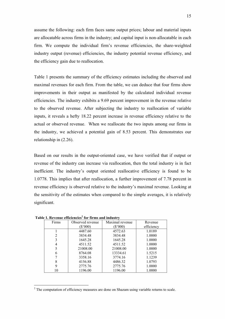
Table 1 presents the summary of the efficiency estimates including the observed and
maximal revenues for each firm. From the table, we can deduce that four firms show
improvements in their output as manifested by the calculated individual revenue
efficiencies. The industry exhibits a 9.69 percent improvement in the revenue relative
to the observed revenue. After subjecting the industry to reallocation of variable
inputs, it reveals a hefty 18.22 percent increase in revenue efficiency relative to the
actual or observed revenue. When we reallocate the two inputs among our firms in
the industry, we achieved a potential gain of 8.53 percent. This demonstrates our
relationship in (2.26).
Based on our results in the output-oriented case, we have verified that if output or
revenue of the industry can increase via reallocation, then the total industry is in fact
inefficient. The industry’s output oriented reallocative efficiency is found to be
1.0778. This implies that after reallocation, a further improvement of 7.78 percent in
revenue efficiency is observed relative to the industry’s maximal revenue. Looking at
the sensitivity of the estimates when compared to the simple averages, it is relatively
significant.
Table 1. Revenue efficiencies2 for firms and industry
Firms Observed revenue ($’000)
Maximal revenue ($’000)
Revenue efficiency
1 2 3 4 5 6 7 8 9
10
4487.60 3834.48 1645.28 4511.52 21008.00 8764.08 3358.16 4156.88 2775.76 1196.00
4572.63 3834.48 1645.28 4511.52 21008.00 13334.61 3774.16 4486.32 2775.76 1196.00
1.0189 1.0000 1.0000 1.0000 1.0000 1.5215 1.1239 1.0793 1.0000 1.0000
2 The computation of efficiency measures are done on Shazam using variable returns to scale.

16
Industry revenue efficiency
(Share-weighted)
1.0969
Industry revenue efficiency (With reallocation of inputs)
1.1822
Efficiency gain (Due to reallocation)
0.0853
Industry revenue reallocative efficiency
1.0778
Industry revenue efficiency Arithmetic Mean
Geometric Mean Harmonic Mean
1.0744 1.0652 1.0576
3. Measures of TFP Growth A wide variety of techniques have been developed for productivity change
measurement. Some are applicable to macro or industry analyses and some to
analyses at micro or firm level. The most commonly used technique in the
measurement of TFP growth is the non-parametric approach. This section gives a
brief review of common non-parametric approaches in firm level productivity
measures and how these measures can be used in measuring aggregate industry TFP
growth.
3.1 Firm level productivity measures In this subsection, we revisit the traditional index number methods for firm level
performance measurement. Following Balk (2001), we also look at the gross output
and value-added approaches in productivity change estimation.
TFP Growth Measurement using Index Numbers We first review the traditional index number formula for measuring productivity
changes in the levels of output produced and the levels of inputs used in the
production process over two time periods.
17
By definition, total factor productivity index measures change in total output relative
to the change in the usage of all inputs. The kth firm TFP index for two time periods s
and t is expressed as
kst
kstk
st IndexInputIndexOutput
TFP lnln = (3.1)
In most empirical applications, the Tornqvist index formula is used for both the output
and input index calculations. Diewert (1992) shows Fisher index satisfies more
properties as compared to Tornqvist index. Fisher index is referred to as an exact and
superlative index, hence it could also be use as another suitable formula to compute
firm’s TFP change. This is given by
kst
kstk
st indexinputFisherindexoutputFisher
TFP = (3.2)
Both Tornqvist and Fisher indices possess important properties and satisfies basic
axioms. In most practical applications, both these indices when used in TFP
measurement yield very similar numerical values. Most statistical agencies involved
in TFP measurement, preferred to use Tornqvist formula.
Gross output and value-added based productivity measures We now consider the productivity concepts and measures discussed in Balk (2001). In
his study, the firm is considered as an input-output system. The commodities
produced by the firm, such as goods and/or services are at the output side while the
commodities consumed such as capital, labour, energy, materials and services inputs
are at the input side.
For any firm k, we let the value of the nominal gross output (GO) during the period t
be equal to the observed revenue. Its production cost (PC) is also equal to the
observed cost. The firm’s value added (VA) can be defined as gross output minus the
cost of intermediate inputs (II). Two important assumptions considered here are: (1)
firm operates in a market environment, so that every commodity comes with a value

18
(in monetary terms) and (2) intermediate inputs are acquired from other firms or
imported.
Balk (2001) defines the firm’s profitability as its revenue divided by its production
cost, that is
Firm profitability = PCGO (3.3)
According to his paper, there is a link between the measurement of productivity levels
and the measurement of productivity growth at the firm level. This link is provided
by the concept of real profitability. If GO is the firm’s total revenue and PC is the
total cost, then GO divided by PC is the firm’s nominal profitability. Hence,
Firm’s Real Profitability = deflatedPCdeflatedGO (3.4)
The above expression is then equivalent to real productivity of the firm. Based on
this, the index of productivity change can be expressed as either a/an:
i) ratio of two productivity levels;
ii) index of real profitability;
iii) index of deflated revenue relative to index of deflated cost ; and/or,
iv) output quantity index divided by an input quantity index.
The productivity level of firm k in period t is then defined as
kt
ktk
t inputaloutputal
TFPRe
Re= . (3.5)
The gross output based TFP index for firm k at period t is measured as
kt
ktk
GOt tproductioninputaloutputgrossal
TFP)cos(Re
Re= . (3.6)
The corresponding firm level value added based TFP index is obtained by
19
kt
ktk
VAt inputslabourandcapitalaladdedvalueal
TFPRe
Re= . (3.7)
The Output-Oriented Malmquist TFP (CCD Approach)
We glance at the general Malmquist productivity index based on Caves, Christensen
and Diewert (CCD)(1982). In here, the Malmquist index is measured using distance
functions. It measures the TFP change between two data points by calculating the
ratio of the distances of each data point relative to common technology. Following
Caves, Christensen and Diewert (1982) approach, under the assumption of technical
and allocative efficiency, we can define a thk firm output-based Malmquist
productivity growth from period s to period t as,
2
1
*
),,,(
kvK
kks
kt
kst
kstk
tks
kt
ks
kO x
xindexinputTornqvistindexoutputTornqvist
xxyyM ∏=
×= . (3.8)
where stskst
kt
k vvv εεεε and ),1()1(* −+−= are local returns to scale in period t
and s. If we have constant return to scale (CRS) in both periods ( i.e. 1== st εε ),
then (3.15) simplifies to
.),,,( kst
kstk
tks
kt
ks
kO indexinputTornqvist
indexoutputTornqvistxxyyM = (3.9)
This would mean that given the assumption that each firm is technically and
allocatively efficient and adding CRS technology then ),,,( kt
ks
kt
ks
KO xxyyM can simply
be computed using the traditional Tornqvist TFP index number formula. The above
result provides a justification for the use of the standard index number measure for
firm level TFP growth analyses.
3.2 Industry level productivity measures We examine different approaches available for aggregating firm level productivity
indices leading to industry-level measures. We also look at the different methods to
calculate the relative sizes of the firms (weights). For all these measures, we assume
20
that all firms in the industry exist during both the comparison and base periods, and
there is no entry or exit of firms.
Simple Averages An easy way to aggregate firm level TFP indices is by the use of simple averaging
procedure. In this aggregation procedure, we are assuming the same (equal) weights
for all the firms in the industry. This is an approach used in some of the DEA program
such as DEAP.
A simple arithmetic, geometric and harmonic mean of all the firm’s TFP growths
between period t and s are given by the following formulas:
.)1(1
1 and ; )( ;
1
1
1
1
∑Π
∑
=
=
= === K
kk
st
Ist
kkst
K
k
Ist
K
k
kst
Ist
TFPK
TFPTFPTFPK
TFPTFP (3.10)
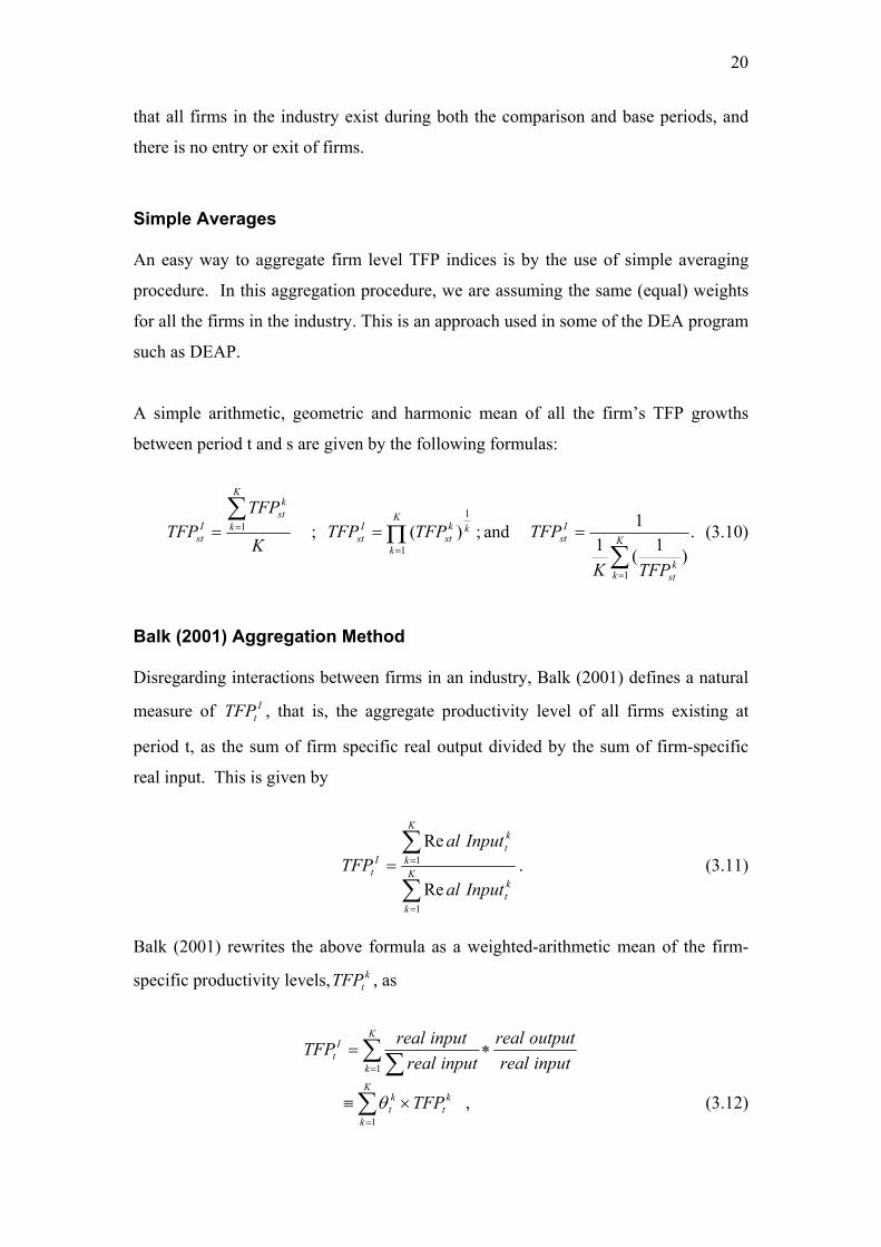
Balk (2001) Aggregation Method Disregarding interactions between firms in an industry, Balk (2001) defines a natural
measure of ItTFP , that is, the aggregate productivity level of all firms existing at
period t, as the sum of firm specific real output divided by the sum of firm-specific
real input. This is given by
∑
∑
=
== K
k
kt
K
k
kt
It
Inputal
InputalTFP
1
1
Re
Re. (3.11)
Balk (2001) rewrites the above formula as a weighted-arithmetic mean of the firm-
specific productivity levels, ktTFP , as
inputrealoutputreal
inputrealinputrealTFP
K
k
It ∗= ∑∑=1
∑=
×≡K
k
kt
kt TFP
1θ , (3.12)

21
where the weights k
tθ are firm-specific real input shares in period t. Note that
∑=
=K
k
kt
1
.1θ
The aggregate productivity change between two period s and t, can be measured as a
difference of ITFP corresponding to those periods, that is,
I
sI
tI
st TFPTFPTFP −=∆ . (3.13) A percentage change is obtained by dividing I
stTFP∆ by IsTFP .
OECD (2001) Following the OECD (2001) Productivity Manual, the aggregate productivity level is
measured as a weighted geometric mean, that is
∏=
=K
k
kt
It
ktTFPTFP
1
)( θ , (3.14)
where k
tTFP and ktθ are defined just like in (3.5) and (3.12) respectively. Taking the
natural logarithmic form of the above expression we can rewrite (3.14) as
k
t
K
k
kt
It TFPTFP lnln
1×= ∑
=
θ . (3.15)
The aggregate productivity change for the industry between periods s and t, is given
by the logarithmic difference
I
sI
tI
st TFPTFPTFP lnlnln −=∆ . (3.16) Fox (2002) aggregation method Assuming that the TFP scores have been calculated using any index number formula,
Fox (2002) constructed a Tornqvist aggregation function to aggregate TFP change.
This is given by

22
−+=∆ ∑
=
K
k
ks
kt
kt
ks
Ist TFPTFPTFP
1)ln)(ln)(
21(exp θθ , (3.17)
where k
sθ is the share of firm k in total industry for period s. It could be noted that
the arithmetic mean of the shares in two periods (s, t) are used to weight (log) changes
in TFP. The share could take on any form (i.e., output share, input share, revenue
share, cost share or valued-added share). Equation (3.17) has a nice property of being
additive, such that the weighted productivity growths for each firm can simply be
added. Moreover, this aggregate measure can be decomposed into the contribution
from each firm and it satisfies the monotonicity property. The only limitation of this
aggregation function is that it is only applicable to an industry where the same set of
firms exists in the two periods.
Weighted averages of firm level productivity We use averaging techniques (3.10), with weights, defined as the arithmetic mean of
the shares of firm k in two periods (s, t), being compared. We can re-express (3.10)
by:
weighted geometric mean of TFP change indices
)
2(
1
)(*kt
ksK
k
kst
Ist TFPTFP
θθ +
=∏= ; (3.18)
weighted arithmetic mean of TFP change indices
kst
K
k
kt
ksI
st TFPTFP )2
(*1∑=
+=
θθ; and, (3.19)
weighted harmonic mean
∑=
×
+=
K
kk
st
kt
ks
Ist
TFP
TFP
1
12
1*θθ
. (3.20)
4. The Firm and Industry Malmquist TFP index
A non-parametric measure that has become popular over the last decade is the data
envelopment analysis (DEA) method. This calculates the Malmquist productivity

23
index based on Fare et al (1994). Subject to availability of suitable panel data, one can
use this frontier estimation method to estimate firm level TFP growth without
requiring any price information. Further, it does not require the assumption that all the
firms are fully efficient, cost minimisers and revenue maximisers. This is of
importance when we are to analyse non-market sectors or non-profit institutions
performances. Another important aspect of DEA is that it permits Malmquist TFP
index to be decomposed into technical efficiency and technical change components.
In this section, we first define the firm level Malmquist TFP index. We assume that:
the firms face the same output prices; all firms face the same technology; all the firms
exist (continuing firm) during all comparison periods; and there is no reallocation of
inputs among firms in the industry. The discussion will be based on the results in
Section 2. We then show how an industry output-oriented Malmquist TFP index can
be defined and derived from firm-specific indexes.
Notation Note that as a notation for this section, vectors with subscripts will represent
observations, thus for instance ),( kt
kt yx denotes the input and output quantities of firm
k in period t. In the analysis, we will use t to denote the ‘comparison period’ and s for
the ‘base period’.
Assuming that all firms face the same technology for any given period t or s, that is
(say at period t), then a firm and industry output (technology set) for period t is simply
defined by )( and )( xPxP Itkkt , respectively. Similarly, we can define a period-s
technology for any firm k and industry as )( and )( xPxP Iskks ,. The above output sets
also satisfies the standard properties.
We now define an output-oriented distance function on the output set Pkt(xk) ,
k=1,2,…,K , as
( ){ }.)(,0:inf),( kktkkkkkkktO xPyyxD ∈>= δδδ (4.1)
Since the outputs are disposable, we then have
1),()( ≤∈ kkktO
kktk yxDiffxPy , (4.2)

24
which means that the distance function, ),( kkktO yxD , will take a value less than or
equal to one if the output vector, yk, is an element of the feasible production set,
Pkt(xk). It will also be increasing in xk and linearly homogeneous in yk. Similarly, we
define an output-oriented distance function for any firm k in period-s on the output set
Pks(xk) , k=1,2,…,K , as
( ){ }.1),(
,)(,0:inf),(
≤
∈>=kkks
O
kkskkkkkkksO
yxD
xPyyxD δδδ (4.3)
Using (2.11), we define an output-oriented distance function for the industry
technology in period-t as
( ){ }
∑∑
∑∑
==
==
∈≤
=>∈=
∈
>=
K
1k1
1
11
1
).( as 1),,...,(
,...,2,10),(: inf max
)(,0:inf),,...,(
xPyyxxD
KkallforxPy
xPyyxxD
ItkK
k
kKItO
kkktkkk
ItK
k
kK
k
kKItO
δδδ
δδδ
δ (4.4)
Similarly, we have an output-oriented distance function for the industry technology in
period-s expressed as ),,...,(1
1 ∑=
K
k
kKIsO yxxD .
Homotheticity
The period-t technology for any firm k exhibits output homotheticity if
)1()()( Nktkktkkt PxGxP = for all kx , where ++ ℜ→ℜNktG : is a non-decreasing
function consistent with the properties of ).( kkt xP This is equivalent to saying that
)(/),1(),( kktkN
ktO
kkktO xGyDyxD = (Balk ,1998).
Implicit Hicks Neutrality
The sequence of k-firms technologies pertaining to periods t=0, 1, 2, 3,… exhibits
implicit Hicks output neutrality if for all kx , ),()(ˆ)( kkkkt xtBxPxP = where
)(ˆ kxP satisfies the properties of )( kkt xP but independent of t. ),( kxtB is also a

25
function satisfying the same properties. It is equivalent to saying that
),1(/),(ˆ),( kk
kkO
kkktO xByxDyxD = (Balk,1998).
4.1 The Firm level Malmquist productivity index
In this section we look at how an industry Malmquist TFP index can be define using
the firm level Malmquist TFP indices. In, short we investigate the possibilities of
aggregating firm level TFP growth measure using the Malmquist TFP index.
Malmquist index formula can be defined using either the output-orientated approach
or the input-orientated approach. This section will also be limited to the output-
orientated approach.
The Malmquist TFP change index Suppose for any firm k, we have sufficient observations in each period (t, s), so that a
technology in each period can be estimated using mathematical programming, then
one would not require the assumptions of technical and allocative efficiency to be
able to calculate the Malmquist TFP index ( Coelli et al (1998). Following Fare et al
(1994), the Malmquist output-oriented TFP change index between the base period-s
and the comparison period-t for any k firm is given by,
21
),(),(
)()(
),,,(
×= k
sk
sktO
kt
kt
ktO
ks
ks
ksO
kt
kt
ksOk
tkt
ks
ks
kO XYD
XYDxyDxyD
xyxyM . (4.5)
This is a geometric mean of two TFP indices. A value of ),,,( kt
kt
ks
ks
kO xyxyM greater
than one indicates positive TFP change from period s to t for firm k. If
),,,( kt
kt
ks
ks
kO xyxyM is less than one then it shows that firm k has a decline in TFP
growth.
Following Fare et al (1994), the kth firm Malmquist output-oriented TFP is defined as
21
),(),(
),(),(
)(),(
),,,(
××= k
sks
ktO
ks
ks
ksO
kt
kt
ktO
kt
kt
ksO
ks
ks
ksO
kt
kt
ktOk
tkt
ks
ks
kO xyD
xyDxyDxyD
xyDxyD
xyxyM , (4.6)

26
where ),( kt
kt
ksO xyD is the distance from the period-t observations to the period-s
technology for any firm k. The first ratio term in the right hand side of equation (4.6)
measures the change in the output-oriented Farrell technical efficiency of firm k
between period s and t. We then write this first component as
),(),(
ks
ks
ksO
kt
kt
ktOk
O xyDxyD
TECchangeefficiencyTechnical == , (4.7)
and the second component which is inside the bracket measures the technical change,
that is,
21
),(),(
),(),(
×== k
sks
ktO
ks
ks
ksO
kt
kt
ktO
kt
kt
ksOk
O xyDxyD
xyDxyD
TCchangeTechnical . (4.8)
This decomposition is easily illustrated using a constant return to scale technology
involving a single output and a single input.
4.2 The industry Malmquist productivity index
Can we define an industry Malmquist TFP index measure which is an aggregate of all
the firm level technical efficiency changes and technical changes?
Suppose we consider an industry with K firms, each firm k producing a single output kjy and a single input k
jx , for any period j, j = s,t. The firms continually exist in the
two periods and all firms assume the same technology in each period j. Moreover, the
input resources are assumed to be fixed, that is, no reallocation of inputs among firms
is allowed in the industry. Then we define an industry Malmquist TFP index by
21
1
1
1
1
1
1
1
1
1
1
1
1
1
1
1
1
),,...,(
),,...,(
),,...,(
),,...,(
),,...,(
),,...,(),...,,,,...,,(
××
=
∑
∑
∑
∑
∑
∑∑∑
=
=
=
=
=
=
==
K
k
ks
Kss
ItO
K
k
ks
Kss
IsO
K
k
kt
Ktt
ItO
K
k
kt
Ktt
IsO
K
k
ks
Kss
IsO
K
k
kt
Ktt
ItO
Ktt
K
k
kt
Kss
K
k
ks
IO
yxxD
yxxD
yxxD
yxxD
yxxD
yxxDxxyxxyM
(4.9)
where,

27
( ){ }
∑∑
∑∑
==
==
∈≤
=>∈=
∈
>=
K
1k1
1
11
1
).( as 1),,...,(
,...,2,10),(: inf max
)(,0:inf),,...,(
tIsk
t
K
k
kt
Ktt
IsO
kkt
kskkt
k
tIs
K
k
kt
K
k
kt
Ktt
IsO
xPyyxxD
KkallforxPy
xPyyxxD
δδδ
δδδ
δ (4.10)
and .,...,1),( :)(),...,()(K
1k 1
1 ∑ ∑= =
=∈=≡== KkxPyyyxPxxPxP kkskt
K
k
kt
kt
ksKtt
Ist
Is (4.11)
Applying the results in Section 2.4 , for a single output case, we can measure the first
component of the right hand side of the equation (4.9) using (2.13), thus
),,...,(
),,...,(
1
1
1
1
IsO
ItO
K
k
ks
Kss
IsO
K
k
kt
Ktt
ItO
stIO TE
TE
yxxD
yxxDTEC ≡=
∑
∑
=
=
. (4.12)
However, for a multi-output case, following (2.14) result, equation (4.12) can be
defined as
),,...,(
),,...,(
1
1
1
1
1
1
ksK
k
ksO
ktK
k
ktO
sIO
tIO
K
k
ks
Kss
IsO
K
k
kt
Ktt
ItO
stIO
osTE
osTE
TETE
yxxD
yxxDTEC
×
×=≡=
∑
∑
∑
∑
=
=∗
∗
=
=
. (4.13)
It could be noted that in the above measure, we need prices for the firm revenue
shares, otherwise we can use shadow shares.
The question now is how to measure industry technical change?
21
1
1
1
1
1
1
1
1
),,...,(
),,...,(
),,...,(
),,...,(
×=
∑
∑
∑
∑
=
=
=
=K
k
ks
Kss
ItO
K
k
ks
Kss
IsO
K
k
kt
Ktt
ItO
K
k
kt
Ktt
IsO
stIO
yxxD
yxxD
yxxD
yxxDTC (4.14)
The problem of measuring technical change for the industry is currently under
investigation. The scope for the use of shadow output shares, in the absence of price
data, are also being considered.
28
4.3 Preliminary aggregation results
In this section, we use the records of 100 individual firms in the Australian textile,
clothing, footwear and leather (TCFL) manufacturing industry, which are taken from
the Australian Bureau of Statistics confidentialised unit record file (ABS-CURF), to
illustrate the sensitivity of the aggregation methods discussed in Section 3. All the
100 firms are continuing firms based on the four-year periods survey results. We also
examine the sensitivity of the results to the use of various industry productivity
changes when we apply different weights in the aggregation of firm level productivity
growths. Lastly, we calculate an aggregate productivity change based on Malmquist
TFP index using geometric average. It could be noted that the data series only
contains four-year period, hence the TFP changes will be limited to three comparison
periods (1996, 1997, and 1998) with 1995 as the base period. Results are presented
only in the form of graphs.
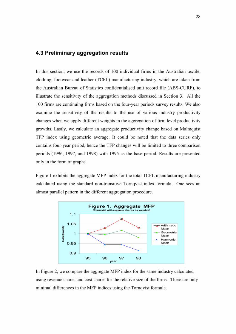
Figure 1 exhibits the aggregate MFP index for the total TCFL manufacturing industry
calculated using the standard non-transitive Tornqvist index formula. One sees an
almost parallel pattern in the different aggregation procedure.
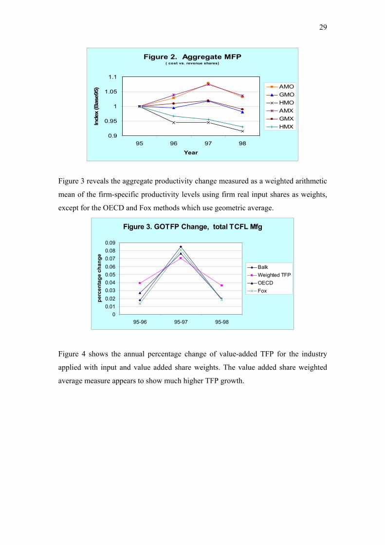
In Figure 2, we compare the aggregate MFP index for the same industry calculated
using revenue shares and cost shares for the relative size of the firms. There are only
minimal differences in the MFP indices using the Tornqvist formula.
Figure 1. Aggregate MFP (Tornqvist with revenue shares as weights)
0.9
0.95
1
1.05
1.1
95 96 97 98year
Inde
x (b
ase9
5) ArithmeticMeanGeometricMeanHarmonicMean
29
Figure 2. Aggregate MFP( cost vs. revenue shares)
0.9
0.95
1
1.05
1.1
95 96 97 98
Year
Inde
x (B
ase9
5)AMOGMOHMOAMXGMXHMX
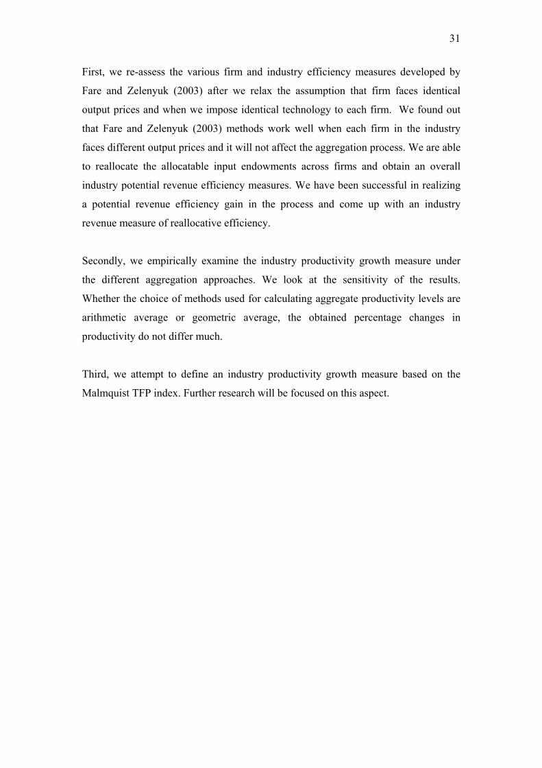
Figure 3 reveals the aggregate productivity change measured as a weighted arithmetic
mean of the firm-specific productivity levels using firm real input shares as weights,
except for the OECD and Fox methods which use geometric average.
Figure 3. GOTFP Change, total TCFL Mfg
00.010.020.030.040.050.060.070.080.09
95-96 95-97 95-98
per
cent
age
chan
ge
BalkWeighted TFPOECDFox
Figure 4 shows the annual percentage change of value-added TFP for the industry
applied with input and value added share weights. The value added share weighted
average measure appears to show much higher TFP growth.

30
Figure 4. VATFP Change, total TCFL Mfg
0
0.05
0.1
0.15
0.2
0.25
0.3
0.35
0.4
95-96 95-97 95-98
perc
enta
ge c
hang
eTFP-Input ShareTFP-VA Shares
Figure 5 depicts the aggregate TFP estimated using the Malmquist TFP index. We
compare the results with the aggregate TFP obtained using the standard Tornqvist
index. We use also cost and revenue shares in aggregating the firm level Malmquist
TFP indices.
Figure 5. Aggregate TFP change - DEA
0.92
0.94
0.96
0.98
1
1.02
1.04
95-96 96-97 97-98Year
Inde
x Revenue SharesCost SharesTFP-Index
5. Concluding Remarks Three major aspects of aggregation have been investigated in this paper.
31
First, we re-assess the various firm and industry efficiency measures developed by
Fare and Zelenyuk (2003) after we relax the assumption that firm faces identical
output prices and when we impose identical technology to each firm. We found out
that Fare and Zelenyuk (2003) methods work well when each firm in the industry
faces different output prices and it will not affect the aggregation process. We are able
to reallocate the allocatable input endowments across firms and obtain an overall
industry potential revenue efficiency measures. We have been successful in realizing
a potential revenue efficiency gain in the process and come up with an industry
revenue measure of reallocative efficiency.
Secondly, we empirically examine the industry productivity growth measure under
the different aggregation approaches. We look at the sensitivity of the results.
Whether the choice of methods used for calculating aggregate productivity levels are
arithmetic average or geometric average, the obtained percentage changes in
productivity do not differ much.
Third, we attempt to define an industry productivity growth measure based on the
Malmquist TFP index. Further research will be focused on this aspect.

32
References
Balk, B.M. (1998), Industrial Price, Quantity and Productivity Indices: The Micro- Economic Theory and an Application, Kluwer Academic Publisher, Boston.
Balk, B.M. (2002), The Residual: On Monitoring and Benchmarking Firms,
Industries, and Economies with respect to Productivity, Inaugural Addresses, Research in Management Series EIA-2001-07-MKT, Erasmus Research Institute of Management, Erasmus University, Rotterdam.
Balk, B., and E. Hoogenboom-Spijker (2003), “The measurement and decomposition
of productivity change: exercises on the Netherlands’ manufacturing industry”, Discussion Paper 03001, Statistics Netherlands, Voorburg.
Blackorby, C., and R. Russell (1999), “Aggregation of efficiency indices”, Journal of
Productivity Analysis, 12(1), 5-20. Bogetoft P. (1999), “Process aggregation and efficiency”, Working Paper,
Department of Economics, Royal Agricultural University, Denmark Briec W., B. Dervaux and H. Lelue (2002), “Aggregation of directional distance
functions and industrial efficiency,” Journal of Economics (Forthcoming) Caves, D.W., L.R. Christensen and W. E. Diewert (1982), “The economic theory of
index numbers and the measurement of input, output and productivity”, Econometrica, 50, 1393-1414.
Coelli, T.J., D.S.P. Rao and G.E. Battese (1998), An Introduction to Efficiency and
Productivity Analysis, Kluwer Academic Publisher, Boston. Fare, R., S. Grosskoft, M. Norris and Z. Zhang (1994), “Productivity growth,
technical progress, and efficiency changes in industrialized countries”, American Economic Review,84,66-83.
Fare, R. and D. Primont (1995), Multi-Output Production and Duality: Theory and
Applications, Kluwer Academic Publishers, Boston. Fare, R., and S. Grosskopf (2002), New Directions: Efficiency and Productivity,
Kluwer Academic Publisher, Boston, (forthcoming). Fare, R., S. Grosskopf and C.A.K. Lovell (1985), The Measurement of Efficiency of
Production, Kluwer Academic Publisher, Boston. Fare, R. and V. Zelenyuk (2003), “On aggregate Farrell efficiencies”, European
Journal of Operational Research, 146, 615-620. Farrell, M.J. (1957), “ The measurement of productive efficiency”, Journal of the
Royal Statistical Society, Series A, CXX, Part 3, 253-290.
33
Fox K.J (1999), “Efficiency at different levels of aggregation: public vs. private sectors firms”, Economic Letters, 65, 173-176.
Fox, K.J (2002), “Problems with (dis)aggregating productivity, and another
productivity paradox”, Draft, School of Economics, The University of New South Wales, Sydney.
Grifell-Tatje, E., and C.A.K. Lovell (1995), “A note on the malmquist productivity
index”, Economic Letters, 47, 169-194. Kumbhakar, S.C. and C.A.K. Lovell (2000), Stochastic Frontier Analysis, Cambridge
University Press,UK. Li, S. K. and Y.C. Ng (1995), “Measuring the productive efficiency of a group of
Firms”, International Advances in Economic Research, 1,377-390.
OECD (2001), Measuring Productivity: Measurement of Aggregate and Industry- Level Productivity Growth, OECD Manual, Paris.
Recommended