Download pdf - On ACTL Formulas Having Linear Counterexamples - … · On ACTL Formulas Having Linear Counterexamples Francesco Buccafurri ... last state and , ... (PSF)|C v It is PSPACE-hard to

Journal of Computer and System Sciences 62, 463�515 (2001)

On ACTL Formulas Having LinearCounterexamples

Francesco Buccafurri

DIMET, Universita� di Reggio Calabria, loc. Feo di Vito, I-89100 Reggio Calabria, ItalyE-mail: bucca�ns.ing.unirc.it

Thomas Eiter and Georg Gottlob

Institut and Ludwig Wittgenstein Labor fu� r Informationssysteme, Technische Universita� t Wien,Favoritenstrasse 9-11, A-1040 Vienna, Austria

E-mail: eiter�kr.tuwien.ac.at; gottlob�dbai.tuwien.ac.at

and

Nicola Leone

Department of Mathematics, University of Calabria, Arcavacata di Rende, I-87030, ItalyE-mail: leone�unical.it

Received November 12, 1999; revised August 18, 2000

In case an ACTL formula , fails over a transition graph M, it is most use-ful to provide a counterexample, i.e., a computation tree of M, witnessing thefailure. If there exists a single path in M which by itself witnesses the failureof ,, then , has a linear counterexample. We show that, given M and ,,where M<% ,, it is NP-hard to determine whether there exists a linear coun-terexample. Moreover, it is PSPACE-hard to decide whether an ACTL for-mula , always admits a linear counterexample if it fails. This means thatthere exists no simple characterization of the ACTL formulas that guaranteelinear counterexamples. Consequently, we study templates of ACTL formulas,i.e., skeletons of modal formulas whose atoms are disregarded. We identifythe (unique) maximal set LIN of templates whose instances (obtained byreplacing atoms with arbitrary pure state formulas) always guarantee linearcounterexamples. We show that for each ACTL formula , which is aninstance of a template #C # LIN, and for each Kripke structure M such thatM<% ,, a single path of M witnessing the failure by itself can be computed inpolynomial time. � 2001 Academic Press

Key Words: model checking; verification; counterexamples; linear coun-terexamples; counterpaths; temporal reasoning; ACTL; branching time logics.

1. INTRODUCTION

ACTL is a well-known particular fragment of Computational Tree Logic (CTL),which is a propositional branching-time temporal logic [2]; see [7, 6] for a rich

doi:10.1006�jcss.2000.1734, available online at http:��www.idealibrary.com on

463 0022-0000�01 �35.00Copyright � 2001 by Academic Press

All rights of reproduction in any form reserved.

background on this and further such logics. ACTL formulas are specified andevaluated over Kripke structures which model finite-state systems. Besides Booleanconnectives, ACTL provides linear-time and branching time operators. The linear-time operators allow for expressing properties of a particular evolution of thesystems given by a series of events in time. Branching time operators allow to takeinto account the existence of multiple possible future scenarios, starting from agiven system state at a point in time. The temporal order defines an evolution tree,which branches from that point towards the future. Thus, every point in time hasa unique past, but, in general, more than one future. Each branch of the treeamounts to a particular evolution series.

The elementary linear-time operators are X (next time), U (until ), and V (unless,releases). Informally, X, means that , is true at the next point in time; ,1U,2

means that there exists a prefix of the computation path such that ,2 is true at thelast state and ,1 is true at all previous states of this prefix; and ,1 V,2 means thattruth of ,1 releases truth of ,2 . Further operators such as F, (sometimes ,), G,(always ,) can be derived from the elementary operators. ACTL has the branchingtime operator A, by which it is possible to express necessary properties for anevolution tree. Informally, A, means that , is true for all branches of the tree. Notethat in full CTL, a dual operator E for expressing possible properties (true alongsome branch) is provided.

1.1. Counterpaths and Linear Counterexamples

The task of an automatic ACTL model checker is the verification of a givenACTL formula , on a Kripke Structure M. In case M does not satisfy , (denotedM<% ,), advanced model checkers (e.g. McMillan's SMV system [11], or thedebugger described by Hojati et al. [9]) provide more information. In particular,as a witness for the failure, a finite representation of an infinite computation path? of M is provided. This path represents a counterexample to , in M. In the idealcase, such a path ? witnesses by itself that M<% ,, in other terms, all informationneeded to disprove that M < , is already contained in ?. In this case, we call ? acounterpath.

To make the above concepts precise, we give in Section 3 a formal definition ofthe concept of counterexample. Roughly, a counterexample to an ACTL formula ,on structure M is a computation tree represented as a multi-path disproving thatM < ,. In case this multi-path has no true branching, and thus actually representsa unique path, we speak about a linear counterexample. A counterpath for , in Mis then the unique path corresponding to a linear counterexample. Note that if thereexists such a counterpath ?, then it holds that M? <% ,, where M? is the Kripkestructure induced by ?, i.e., the structure whose states are all those states of M thatalso occur in ?, where the states are, moreover, labeled by the same labels as in M,and whose transitions are those that occur in ?.

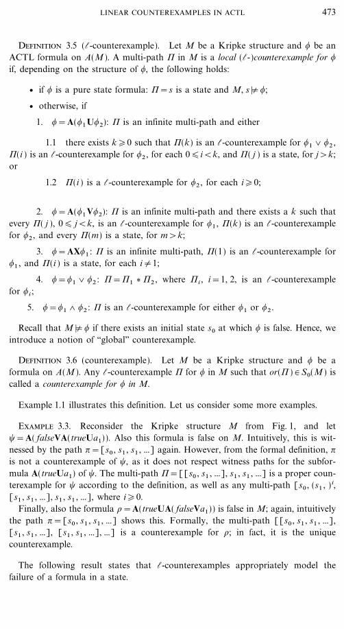
Example 1.1. Let M amount to the transition graph in Fig. 1, where initialstates are colored black, and consider the formula ,=A(trueUa1), which can beabbreviated as AFa1 .

464 BUCCAFURRI ET AL.

FIG. 1. Transition graph representing structure M (initial state s0).

It holds that M<% ,: Along the path ?=[s0 , s1 , s1 , ...], the atom a1 is false ateach stage ?(i ) of ?, i�0. This implies M, ? < cFa1 . Thus, ? witnesses the failureof , in M. Note that the information contained in ? alone is sufficient for disprov-ing ,; we do not have to consider elements of M (states or transitions) outside ?to show that M<% ,. Thus ? is a counterpath of ,.

1.2. Linear Counterexamples May Not Exist

A counterpath provides very useful, compactly presented, and self-containedinformation to a system designer or verifier, allowing him or her to locate a designerror in a most comfortable way. It would thus be most desirable to be able tocompute a (representation of a) counterpath in polynomial time whenever anACTL formula , fails over a structure M.

Unfortunately, as shown by the example below, if M<% ,, a counterpath (or,equivalently, a linear counterexample) does not necessarily exist.

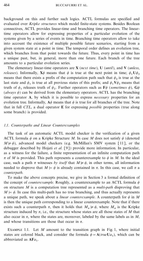
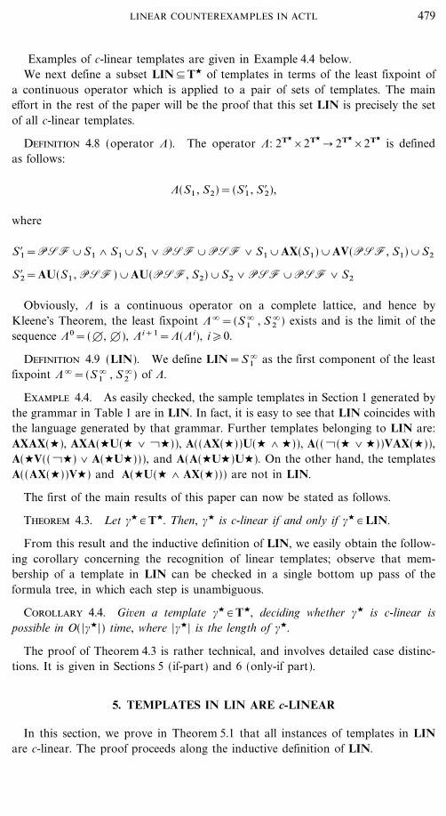
Example 1.2. Let M amount to the transition graph in Fig. 2, and consider,=A(trueUA( falseVa)), which can be abbreviated as AFAGa. It is easy to verifythat M<% ,. Indeed, there is a path ?=[s0 , s0 , ...] starting from the initial statewhere always the nested formula AGa does not hold, as, for each i�0, there existsa path starting at ?(i ) where sometimes a is not true (e.g., on the path?$=[s0 , s1 , s2 , s2 , ...] a is not true at s1). The path ? itself is not a complete coun-terexample. To disprove that M < ,, it is necessary to consider a further path foreach state of ? (here always s0) in order to show that the subformula AGa does nothold. This gives rise to a multi-path 6, which we write as follows: 6=[[s0 , s1 , s2 ,s2 , ...], [s0 , s1 , s2 , s2 , ...], ...]. It consists of a computation tree with main branch[s0 , s0 , ...] in which at each stage a branch [s0 , s1 , s2 , s2 , ...] starts. This multi-path6 is a counterexample for , in M, and not the single path ?. Note that 6 is nota linear counterexample, but a truly branching infinite tree. Note, furthermore, thatno single path is a counterexample for ,. Therefore, no linear counterexample existsin this case, and thus no counterpath witnessing that M<% , exists.

Besides the above very simple example, many other cases can be found in whicheach counterexample is a truly branching computation tree. They include formulasof the shape AF, 6 AF� (e.g., AFa1 6 AFa2 on the structure M in Fig. 1),AF(AG, 6 AGc,), which informally states that any evolution must commit at

FIG. 2. Another transition graph representing structure M (initial state s0).

465LINEAR COUNTEREXAMPLES IN ACTL

some point about a condition , being true or false, and AF, 6 AG�, which statesthat either , becomes true at some stage or � always holds.

From these observations, we can infer that in many cases a simple ``counter-example path'' output by an ACTL model checker such as McMillan's system [11]can not be a full counterexample, but only one path��usually the main path or``backbone''��of a counterexample. Such a path may help to track the design orimplementation error, but it does by itself not necessarily explain why the formulafails, and one may need to consider states and transitions outside that path in orderto track the flaw. The debugger in [9] constructs a counterexample for an ACTLformula , unwinding the formula. A counterpath would be desirable, since theunwinding can be done along it, without reference to other parts of the structure.

1.3. Main Research Questions Addressed

Given that linear counterexamples (and counterpaths) are useful, but do notalways exist, the following questions naturally arise:

v Is there an efficient method of deciding whether an ACTL formula , has alinear counterexample (and thus a counterpath) on a given Kripke structure M,where M<% ,?

v Is there a simple characterization of those ACTL formulas which guaranteelinear counterexamples? In other terms, is there an efficient method for tellingwhether a formula , has the property that whenever M<% , holds for a structureM, then there exists a linear counterexample (and thus a counterpath) witnessingthis?

v If the above fails, how can we efficiently identify large classes of formulasthat guarantee linear counterexamples?

v Can we efficiently compute linear counterexamples in case they exist (and,related to this, efficiently recognize them) ? If this is not generally possible, thenmaybe for large classes of ACTL formulas?

1.4. Main Results

Our main results are shortly summarized as follows:

v We give, in Section 2, a precise definition of the concepts of linear coun-terexample and of the related concept of counterpath.

v We show that given M and ,, where M<% ,, it is NP-hard to determinewhether there exists a linear counterexample (Theorem 4.2).

v As a consequence, even in case counterpaths exist, computing a counterpathis a hard problem. Therefore, unless NP=P, for every ACTL model-checker MC

that works in polynomial time and produces ``single-path counterexamples'' in caseof failure, there exist infinitely many Kripke structures M and formulas ,, such thatM<% , and the counterexample path output by MC represents a partial (and nota complete) counterexample even though there exists a counterpath (i.e., a pathrepresenting a complete counterexample).


TABLE 1

BNF Grammar for Linear Templates

LIN ::= PSF | (LIN7 LIN) | (LIN6 PSF) | (PSF6 LIN) | AX(LIN) | A(PSF V LIN) | ULINULIN ::= A(LIN U PSF) | A(PSF U ULIN) | (ULIN 6 PSF) | (PSF6 ULIN)

PSF ::= (PSF 7 PSF) | (PSF 6 PSF) | c(PSF) | C

v It is PSPACE-hard to decide whether an ACTL formula , in case of failurealways admits a linear counterexample (Theorem 4.1). This means that there existsno simple characterization of the ACTL formulas that guarantee linear coun-terexamples.

v Consequently, we study templates of ACTL formulas, i.e., skeletons ofmodal formulas whose atoms are disregarded and replaced by the symbol C. Asmain result of this paper, we identify the (unique) maximal set LIN of templateswhose instances, obtained by replacing C's with arbitrary pure state formulas,always guarantee linear counterexamples (Theorem 4.3). The set LIN of templatesis given by the BNF grammar in Table 1. For example, the templates AX(C),A(CVAX(C))), and (C 7 A(CVAX(C))) are in LIN, as well as A(CUC), A(CUA(CUC)), and A(A(CVAX(C))U(C 7 C)). On the other hand, the templateA(CUA(CVC)) of the formula ,=A(trueUA( falseVa)) in Example 1.2 is not inLIN, and also the template A(CUC) 6 A(CUC) of the formula A(trueUa1) 6A(trueUa2)=AFa1 6 AFa2 mentioned above is not in LIN.

Obviously, it is recognizable in polynomial time (and in fact in linear time)whether a template belongs to LIN, and whether an ACTL formula , is an instanceof some template in LIN. In particular, we prove:

V If , is an instance of a template #C # LIN, then, for each structure M suchthat M<% ,, there exists a linear counterexample, and thus a counterpath in Mwitnessing this failure.

V If #C is a template not contained in LIN, then there exist an instance , of#C and a structure M such that M<% , but there exists no linear counterexample for, in M.

v We show that for each ACTL formula , which is an instance of a template#C # LIN, and for each Kripke structure M such that M<% ,, a counterpath, i.e., asingle path of M witnessing the failure, can be computed in polynomial time(Theorem 5.2).

v Finally, we show that recognizing a valid counterpath for an arbitraryACTL formula , is possible in polynomial time. This follows from the fact that theproblem can be easily reduced to a model checking problem M$<,, which can besolved in polynomial time (Theorem 5.3).

Note that it could be the case that systems like McMillan's do always yield avalid counterpath in case the input formula , is an instance of a template in LIN,i.e., they would be (sound and) complete for generating counterpaths on the class


of LIN instances. Our results may serve as a starting point for determining theexact ACTL fragments on which such systems are complete with respect to genera-tion of counterpaths. Furthermore, the a priori knowledge that linear counter-examples do always exist for instances of LIN templates may be exploited in thedesign of more efficient algorithms than those which handle the general case ofarbitrary ACTL formulas like the one employed in McMillan's system. These issuesare beyond the scope of the paper and left for further work.

1.5. Structure of the Paper

After this introduction, some preliminaries and notation are given in Section 2. InSection 3, the formal definition of counterexamples is provided, for which multi-paths are introduced. Thereafter, we turn our attention in Section 4 to linear coun-terexamples and multi-paths. After proving that recognizing linear ACTL formulasis intractable, we define the class LIN of templates; furthermore, we formally statethe characterization of c-linear templates, which is the first main result of thispaper. Sections 5�6 are devoted to the proof of this result and to the computationof counterpaths for LIN-instances, which is the second main result. The paper isclosed in Section 7 with a discussion and an outlook on future work.

2. PRELIMINARIES

Definition 2.1 (ACTL formulas). Let A be a set of atomic propositions. Then,ACTL is the set of state formulas on A inductively defined as follows:

(1) Any Boolean formula over atoms from A built using the connectives7 , 6 , and c is a pure state formula; a pure state formula is a state formula;

(2) if , and � are state formulas, then (, 6 �), and (, 7 �) are state for-mulas;

(3) if , and � are state formulas, then X,, ,U� and ,V� are path formulas;

(4) if , is a path formula, then A(,) is a state formula.

Intuitively, path formulas describe properties of evolution series because they usetemporal operators next time, until, and unless.

Notation. For any sets D1 and D2 of formulas, we shall use the followingnotation:

AX(D1) = [AX(#) | # # D1],

AU(D1 , D2)=[A(#1U#2) | #1 # D1 , #2 # D2],

AV(D1 , D2) = [A(#1 V#2) | #1 # D1 , #2 # D2],

D1 7 D2 = [(#1 7 #2) | #1 # D1 , #2 # D2],

D1 6 D2 =[(#1 6 #2) | #1 # D1 , #2 # D2].


Given a formula , or a set S of formulas, we will denote by AP(,) (resp., AP(S))the set of atomic propositions occurring in , (resp., S). We will use true and falseas shorthand for pure state formulas which are tautologies and contradictions,respectively. We shall omit or add parentheses in formulas following the usual con-ventions.

The formal definition of the semantics of ACTL refers to particular Kripkestructures. Informally, they are finite transition graphs with labeled states.

Definition 2.2 (Kripke Structure). A Kripke structure is a quintuple M=(A,S0 , S, R, L) such that:

v A is a finite set of atomic propositions, denoted A(M );

v S is a finite set of states, denoted S(M);

v S0 �S is a finite set of initial states, denoted S0(M);

v R�S_S is a transition relation, denoted R(M );

v L: S � 2A is a mapping assigning to each state of S the set of atomicpropositions true in that state; L is called label function, and is denoted by L(M ).

For convenience, we often denote by Ms the Kripke structure which is identicalto M except S0(Ms)=[s] where s # S(M ), i.e., s is the unique initial state. Further-more, we will sometimes focus on structures M such that S0(M)=[s0] and(s, s0) � R(M ), for all s # S(M ), i.e., M has a unique initial state s0 , and s0 is notreachable from any state in M. We refer to such structures as conic.

Note that many authors (e.g. [7, 10]) require that the transition relation R(M)in a Kripke structure M is total, i.e. \s _s$.R(s, s$) holds. This restriction would letthe main results of this paper unaffected. We shall come back to this issue anddiscuss it in more detail in Section 7.

The dynamic temporal evolution is modeled by infinite paths in the Kripkestructure.

Definition 2.3 (path). A path ? of a Kripke structure M is an infinite sequence?=[s0 , s1 , ..., si , ...] such that for each i�0 (si , si+1) # R(M ). Given an integeri�0 and a path ? we denote by ?(i ) the (i+1)-th state of ?.1 Thus, the first stateof a path ? is denoted by ?(0). Given an integer j�0 and a path ?, the j-suffix ? j

of ? is the path [?( j ), ?( j+1), ...]. Clearly, ?=?0 and ?(i )=?i (0).

The semantics of ACTL is now defined through an entailment relation <, whichcan be applied on states s and paths ? for evaluating state and path formulas,respectively.

Definition 2.4 (satisfaction). Let s and ? be a state and a path in M, respec-tively. Then, the satisfaction relation < for state and path formulas, respectively, ona Kripke structure M is inductively defined as follows.

1. M, s<p, if p # L(M )(s) for any atomic proposition p # A;

2. M, s<c,, if M, s<% , where , is a state formula;


1 Thus, the first state of a path ? is denoted by ?(0).

3. M, s<,1 6 ,2 , if M, s<,1 or M, s<,2 where ,1 and ,2 are state for-mulas;

4. M, s<,1 7 ,2 , if M, s<,1 and M, s<,2 where ,1 , ,2 are state formulas;

5. M, s<A(�), if M, ?<� for all paths ? in M such that ?(0)=s;

6. M, ?<X,, if M, ?(1)<,;

7. M, ?<,1 U,2 , if there exists an integer k�0 such that M, ?(k)<,2 andM, ?( j )<,1 for all 0� j<k;

8. M, ?<,1 V,2 , if for every k�0 it holds that M, ?( j )<% ,1 for all 0� j<kimplies M, ?(k)<,2 .

We write M<, if M, s0 <,, for every initial state s0 # S0(M).

Intuitively, a state formula holds along a path, if it is true at its first state; ,1U,2

is true, if ,1 is true along the path until some state is reached at which ,2 is true;and ,1V,2 is true, if there is no stage such that ,2 is false and ,1 is false at all pre-vious states. Note that U and V are dual operators: ,1U,2 is true precisely ifc,1 Vc,2 is false.

3. MULTI-PATHS AND COUNTEREXAMPLES

If an ACTL formula , is not true in a structure M, then there must be someevidence which proves the failure of the formula. For a pure state formula ,, aninitial state s0 at which , is false is a witness of this fact; if , is of the form AX�,where � is a pure state formula,then a path ? starting at some s0 # S0 such that �is false at ?(1) is such a witness. The falsity of formulas A(,1U,2), A(,1V,2) wherethe ,i are pure state formulas is witnessed similarly by a path ?.

Intuitively, a path ? as described is a counterexample for the truth of , in M. Itappears that for more complex formulas , which involve nested A quantifiers, asingle path ? may not be by itself witness that , fails in M. To formally capturethis, nesting of paths must be taken into account. This motivates the definition ofmulti-paths, which serve as a basis for a formal definition of counterexamples [1].

3.1. Multi-Paths

Informally, a multi-path represents an infinite tree T, which has a designatedbranch as a backbone (called main path). The branches of the tree which spring offfrom the main path at a certain stage are collected in a tree, which is recursivelyrepresented as a multi-path. Thus, multi-paths can be inductively defined. Observethat this representation of a tree is different from the usual inductive definition inwhich a tree is built by assigning child nodes to a parent node. The main advantageof the multi-path concept is the preservation of the nesting of paths, which is lostin the standard tree definition.

Preliminary to the formal definition of multi-paths, we introduce multi-sequences.


FIG. 3. Branching paths.

Definition 3.1 (multi-sequence). Let S be a set of states. Then,

v for every state s # S, 6=s is a finite multi-sequence in S;

v if 60 , 61 , ... are countably infinitely many multi-sequences in S, then6=[60 , 61 , ...] is a multi-sequence in S.

For any multi-sequence 6, its (i+1)-th element is denoted by 6(i ), for all i�0;2

moreover, its origin, denoted or(6 ), is or(6 )=s, if 6=s is a single state, andor(6 )=or(6(0)), otherwise.

Next we introduce the notion of main sequence of a multi-sequence. Informally,it is the sequence formed by the origins of all elements in a multi-sequence.

Definition 3.2 (main-sequence). For any multi-sequence 6, the main sequenceof 6, denoted by +(6 ), is

v s, if 6=s is finite;

v the sequence [or(6(0)), or(6(1)), or(6(2)), ...], otherwise.

Multi-paths are multi-sequences which model nested paths in M.

Definition 3.3 (multi-path). A multi-sequence 6 is a multi-path in M, if either6 is finite, or +(6 ) is a path in M and for every i�0, 6(i ) is a multi-path in M.

The main sequence of a multi-path 6 is called the main path of 6.

Note that multi-paths generalize paths. Indeed, a path can be seen as an infinitemulti-path 6 such that each element 6(i ) is a state.

An infinite multi-path 6 represents intuitively an evolving computing tree, whosebranches are the main path +(6 ) and all paths of form ?0?1 where ?0=+(6 )(0), ...,+(6 )(i&1) is a finite prefix of +(6 ) and ?1 is a branch of the multi-path 6(i ),where 6(i ) must be infinite.

Example 3.1. Assuming proper M, the multi-sequence 6=[[s0 , s1 , s1 , ...],s2 , s2 , ...] is a multi-path, which represents two paths ?1=[s0 , s1 , s1 , ...] and?2=[s0 , s2 , s2 , ...] starting at s0 (Fig. 3). ?2 is the main path +(6 ) of 6. The multi-path 6=[[s0 , s1 , s1 , ...], s2 , [s0 , s1 , s1 , ...], s2 , [s0 , s1 , s1 , ...], ...] has main path+(6 )=[s0 , s2 , s0 , s2 , ...] and represents the computation tree in which from +(6 )at every even stage +(6 )(2k) a path [s0 , s1 , s1 , ...] branches off; hence, 6 containsbesides +(6 ) all paths of form [(s0 , s2) i, s0 , s1 , s1 , ...], i�0.


2 Thus, 6(0) is the first element of the multi-sequence 6.

An important note is that in general, a multi-path 6 may not directly reflect inits structure a truly branching computation tree. In fact, the definition allows fakebranching, in the sense that two nested branching paths may amount to the samepath in the structure. For example, in the multi-path 6=[s0 , s1 , [s2 , s3 , s4 , ...], s3 ,s4 , ...], the branch s2 , s3 , s4 , ... is identical to the remainder of the main path s2 , s3 ,s4 , ... . This is not a shortcoming of our definition, but an important feature; itallows to express that a particular path is a subpath of another one. In an extendedvocabulary for multi-paths, this could be expressed more elegantly; however, wedisregard such an extension here. Note that for our purposes, we can restrict tomulti-paths which have effective finite representations [1].

3.2. Counterexamples

We are now prepared to formalize the notion of counterexample. Intuitively, acounterexample for a formula , is a special multi-path 6 originating at an initialstate demonstrating the falsity of ,. Since counterexamples are defined inductively,we need the concept of a local counterexample, which may origin at an arbitrarystate rather than an initial state. For the technical definition of local counterexam-ples, we use an operation for merging two multi-paths into a single one.

Definition 3.4 (merge). Let 61 and 62 be two multi-paths such thator(61)=or(62). The merge of 61 and 62 , denoted by 61 V 62 , is the multi-pathrecursively defined as follows:

61 V 62={61

[61 V 62(0), 62(1), 62(2), ...]if 62 is finite;otherwise.

Intuitively, the trees represented by 61 and 62 are merged at their common root.

Example 3.2. Merging 6=[[s0 , s11, s12

, ...], s21, s23

, ...] and 6$=[s0 , s31, s32

, ...]yields

6 V 6$=[6, s31, s32

, ...]=[[[s0 , s11, s12

, ...], s21, s22

, ...], s31, s32

, ...], while

6$ V 6=[6$ V [s0 , s11, s12

, ...], s21, s22

, ...]

=[[6$, s11, s12

, ...], s21, s22

, ...]

=[[[s0 , s31 , s32 , ...], s11 , s12 , ...], s21 , s22 , ...].

The two merges essentially represent the same branching of three paths?i=[s0 , si1 , si2 , ...] for i # [1, 2, 3], starting from s0 .

Note that +(61 V 62)=+(62) in case 62 is infinite and +(61 V 62)=+(61)otherwise. We remark that merging 61 and 62 by adding 61 as first element to 62

does not work, since in general, this leads to a set of paths different from those in61 and 62 ; the result may even not be a multi-path.


Definition 3.5 (l-counterexample). Let M be a Kripke structure and , be anACTL formula on A(M ). A multi-path 6 in M is a local (l-)counterexample for ,if, depending on the structure of ,, the following holds:

v if , is a pure state formula: 6=s is a state and M, s<% ,;

v otherwise, if

1. ,=A(,1U,2): 6 is an infinite multi-path and either

1.1 there exists k�0 such that 6(k) is an l-counterexample for ,1 6 ,2 ,6(i ) is an l-counterexample for ,2 , for each 0�i<k, and 6( j ) is a state, for j>k;or

1.2 6(i ) is a l-counterexample for ,2 , for each i�0;

2. ,=A(,1V,2): 6 is an infinite multi-path and there exists a k such thatevery 6( j ), 0� j<k, is an l-counterexample for ,1 , 6(k) is an l-counterexamplefor ,2 , and every 6(m) is a state, for m>k;

3. ,=AX,1 : 6 is an infinite multi-path, 6(1) is an l-counterexample for,1 , and 6(i ) is a state, for each i{1;

4. ,=,1 6 ,2 : 6=61 V 62 , where 6i , i=1, 2, is an l-counterexamplefor ,i ;

5. ,=,1 7 ,2 : 6 is an l-counterexample for either ,1 or ,2 .

Recall that M<% , if there exists an initial state s0 at which , is false. Hence, weintroduce a notion of ``global'' counterexample.

Definition 3.6 (counterexample). Let M be a Kripke structure and , be aformula on A(M ). Any l-counterexample 6 for , in M such that or(6 ) # S0(M ) iscalled a counterexample for , in M.

Example 1.1 illustrates this definition. Let us consider some more examples.

Example 3.3. Reconsider the Kripke structure M from Fig. 1, and let�=A( falseVA(trueUa1)). Also this formula is false on M. Intuitively, this is wit-nessed by the path ?=[s0 , s1 , s1 , ...] again. However, from the formal definition, ?is not a counterexample of �, as it does not respect witness paths for the subfor-mula A(trueUa1) of �. The multi-path 6=[[s0 , s1 , ...], s1 , s1 , ...] is a proper coun-terexample for � according to the definition, as well as any multi-path [s0 , (s1 , ) i,[s1 , s1 , ...], s1 , s1 , ...], where i�0.

Finally, also the formula \=A(trueUA( falseVa1)) is false in M; again, intuitivelythe path ?=[s0 , s1 , s1 , ...] shows this. Formally, the multi-path [[s0 , s1 , s1 , ...],[s1 , s1 , ...], [s1 , s1 , ...], ...] is a counterexample for \; in fact, it is the uniquecounterexample.

The following result states that l-counterexamples appropriately model thefailure of a formula in a state.


Theorem 3.1 [1]. Let M be a Kripke structure, , a formula on A(M), ands # S(M). Then, M, s<% , if and only if there exists an l-counterexample 6 for ,such that or(6 )=s.

Corollary 3.2 [1]. For any Kripke structure M and formula , on A(M),M<% , if and only if there exists a counterexample 6 for , in M.

As discussed earlier, in many cases a counterexample for a formula is (essentially)a single path. This is true e.g. for the formulas considered in the Examples 1.1 and3.3. However, as Example 1.2 and the following example show, there are differentcases in which a truly branching tree is needed.

Example 3.4. Consider the structure M as in Fig. 1 again, but now the formula,=A(trueUa1) 6 A(trueUa2). Clearly, M<% ,: For every ai , i=1, 2, there is aninfinite path ?i=s0 , si , si , ... which never reaches a state at which ai is true; hence,every disjunct AFai in , is false. A counterexample for , is the multi-path6=[[s0 , s1 , s1 , ...], s2 , s2 , ...], which results by merging the ? i 's into 6=(?1 V ?2).Notice that no counterexample for , exists that is an ordinary path, and that?1 V ?2 , ?2 V ?1 are the only (isomorphic) counterexamples for ,.

4. LINEAR COUNTEREXAMPLES

In this section, we formalize our intuition of a single path counterexample fromthe previous section. For this purpose, we introduce first the concept of a linearmulti-path. Such a path is built over a single path in the structure, which exactlyprescribes the next state in each transition throughout the multi-path.

4.1. Linear Counterexamples and c-Linear Formulas

Definition 4.1 (linear multi-path). A multi-path 6 is linear, if one of thefollowing applies:

1. 6 is finite (i.e., a single state); or

2. for each i�0, either

2.1 6(i ) is a state, or

2.2 +(6(i )) coincides with +(6 )i (the i-suffix of +(6 )) and 6(i ) is linear.

Informally, a multi-path is linear if the main paths of its elements are suffixes ofits main path, and this is recursively true also for the multi-paths of the sequence.Thus, while in general, multi-paths represent evolutions with branching, linearmulti-paths have only artificial branching, and represent essentially a single path.

Example 4.1. Consider the multi-path

6=[s0 , s1 , s2 , s3 , [s4 , s5 , s4 , [s5 , s4 , s5 , s4 , ...], s4 , s5 , ...], s5 , s4 , s5 , s4 , ...].

As can be seen, this multi-path is linear. The path [s5 , s4 , s5 , s4 , ...] nested into6(4)(3) represents a path branching from the main path of 6(4). However, this


path coincides with the suffix +(6(4))3 of the main path of 6(4). Hence, it does notrepresent an alternative evolution. In this sense, a linear multi-path represents onlylinear evolutions.

Observe that the multi-path 6$=[[s0 , s1 , s2 , s3 , s2 , s3 , ...], s4 , s5 , s6 , s5 , s6 , s5 , ...]is not linear.

We remark that we could have equivalently defined linear multi-paths in termsof bisimilarity of branching computations. Recall that two processes are (weakly)bisimilar [12], if there exists some bisimulation on them, i.e., a binary relation B onprocesses such that whenever B(P, Q) and P can perform some transition : tobecome P$, then Q can perform the same transition : to become some Q$ such thatB(P$, Q$) holds, and, vice versa, if Q can become Q$ by some transition :, then Pcan become some P$ by transition : such that B(P$, Q$) holds. Every infinite multi-path 6 (thus, also every path) represents a process P that can become the process[6(1), 6(2), ...] by the transition :=or(6 ) and any process P$ that 6(0) canbecome (by the same transition). We may then call an infinite multi-path 6 linear,if it is bisimilar to some (simple) path ?. This notion of linearity is, as easily seen,equivalent to the one in Definition 4.1; in fact, under this notion 6 is linear if andonly if it is bisimilar to its main path +(6 ).

Definition 4.2 (linear counterexample and counterpath). A counterexample 6for an ACTL formula , in a structure M is linear, if 6 is a linear multi-path. Themain path +(6 ) of any linear counterexample 6 for , in M is a counterpath for ,in M.

As easily verified, the counterexamples for the formulas presented in Examples1.1 and 3.3 are linear counterexamples, and the `ìntuitive'' counterexamples thereare the respective counterpaths.

As for counterexamples, it is of particular interest to have a linear counterexam-ple at hand, since such a counterexample is in generally easier to understand thanan arbitrary counterexample. Moreover, the description of such counterexamplescan be simplified. Observe that McMillan's SMV procedure [11] returns a singlepath ? rather than a counterexample as used here when an ACTL formula fails.This path plays a similar role as the main path of our notion of a counterexample6. If 6 and ? grasp the same witness, then +(6 ) should coincide with ?, and itcontains in fact all relevant information which is needed for witnessing the failureof ,. From ?, a counterexample respecting the (artificial) branching of paths asrequired from the structure of , can be reconstructed.

We thus direct our attention to the existence of linear counterexamples.

Definition 4.3 (c-linear). An ACTL formula , is c-linear, if M<% , implies thata linear counterexample for , exists in M, for every Kripke structure M.

4.2. Complexity of Recognizing c-Linear Formulas

Unfortunately, recognizing c-linear formulas is complex in general, which isexpressed by the following result.


Theorem 4.1. Deciding whether a given ACTL formula , is c-linear isPSPACE-hard.

Proof. This result is proved by a reduction from the unsatisfiability problem forACTL formulas on structures M where R(M ) is total. This problem is PSPACE-complete by results of Kupferman and Vardi (see [10]).

Let , be an arbitrary ACTL-formula, and let a be a fresh atom not occurringin ,. Let the formula � be defined as follows:

�=AXa 6 AX(ca 7 ,).

It holds that � is c-linear if and only if , is unsatisfiable over structures M whereR(M ) is total.

To prove this, suppose first that , is unsatisfiable over all M where R(M ) is total.Let M be any structure (where R(M) is not necessarily total) such that M<% �. Thisimplies that AXa has a counterexample in M, which is a simple path ? representedby a pair P, C where P is a path (prefix) and C a cycle in M. The assumption on, implies that ca 7 , is globally false (and in particular, at ?(1)) in the structureM? which is naturally induced by ? in M. Consequently, ? is a counterpath for �in M? , and thus also in M. This means that � is c-linear.

Now suppose that , is satisfiable on some structure M$ with total R(M$). Hence,a state s$0 # S0(M$) exists such that M$, s0 $<,. Let M be the structure corre-sponding to the transition graph in Fig. 4.

It holds that M<% �. Indeed, every path ?1=[s0 , s$0 , ...] is a counterpath for�1=AXa, and the path ?2=[s0 , s1 , s1 , ...] is a counterpath for �2=AX(ca 7 ,);thus, their merge 6=?1 V ?2 is a counterexample for �. Clearly, any counter-example for � in M must contain both s$0 and s1 ; thus, a linear counterexamplefor � in M is impossible, which means that � is not c-linear. K

This result implies that a polynomial-size and polynomial-time checkable proofwitnessing that a formula is c-linear is illusive, and thus we may abandon the searchfor an appealing syntactical characterization of c-linear formulas.

A related, in practice perhaps more important issue is whether the existence of alinear counterexample for a formula can be efficiently decided ad hoc, i.e., given anACTL formula , and a structure M, decide whether , has a linear counterexamplein M (and, if so, return a counterpath represented in a suitable way). As it turnsout, also this problem is intractable.

Theorem 4.2. Given a Kripke structure M and an ACTL-formula ,, decidingwhether , has a linear counterexample (equivalently, a counterpath) in M is NP-hard.

FIG. 4. Structure M for �=AXa 6 AX(ca 7 ,) (initial state s0).


Proof. We describe a polynomial-time transformation of deciding whether agiven directed graph G=(V, E ) has a Hamiltonian circuit, which is well-knownNP-complete [8], into this problem. Recall that a Hamiltonian circuit is asequence C=vi1 , ..., vin of all the vertices V=[v1 , ..., vn] such that an edge isdirected from vij to vij+1

and from vin to vi1 .We construct M and , as follows. The set S of states of M is V, which is also

the set A of atomic propositions and the set S0 of initial states. The transition rela-tion R is E, and each v # V has the label L(v)=[v].

The formula , is as follows:

,=A \trueU \ �v # V \v 7 �

w # V"[v]

AXA(vVcw)+++ .

Intuitively, a linear counterexample for , in M is an infinite path ? such that ineach state ?(i )=v, the path must be continued in states ?(i+1), ?(i+2), ..., suchthat all other vertices w{v appear before v may reappear.

We claim that G has a Hamiltonian circuit if and only if , has a counterpath in M.

(O) Let C=vi1 , ..., vin be a Hamiltonian circuit of G. We claim that the path?=(vi1 , vi2 , ..., vin)

� is a counterpath of ,. To verify this, we have to show that theformula

�v # V

�v , where �v=v7 \ �w # V"[v]

AXA(vVcw)+is false in each state ?(i ), i�0, and that a local counterexample witnessing this factcan be built over ?i.

For each v # V such that v{?(i ), v is false at ?(i ) and thus ?(i ) is a local coun-terexample for �v over ?i. For the v # V such that v=?(i ), we must show that foreach w # V"[v], the suffix ?i is a local counterpath of the formula AXA(vVcw);that is, that the suffix ?i+1 is a local counterexample of A(vVcw). Clearly, this istrue for the w # V"[v] such that w=?(i+1); any w$ # V"[v, w] occurs as ?(i+k),where 1<k<n, and v is false at ?(i+k&1); thus, ?i+1 is a local counterexamplefor A(vVcw). This proves that �v # V �v is false in ?(i ), and that ?i is a local coun-terpath for each AXA(vVcw) where w # V"[v]. Thus, ? is a counterpath for ,in M.

(o) Suppose that , has a counterpath ? in M. We show that the prefix?(0), ..., ?(n&1) of ? is a Hamiltonian circuit of G. Let v # V be the node such that?(0)=v. Then, ? is a counterpath for the formula �v from above. This implies that? is a counterpath for the formula AXA(vVcw), for each w # V"[v]. Thus, ?1 isa local counterpath for A(vVcw). Hence, w must occur in ?, and v must be falsein each state ?(i ) where 1�i<kw and ?(kw) is the first occurrence of w in ?. Conse-quently, ?(n) is the first possible position for a second occurrence of v in ?.

Now consider wi=?(i ), where i>0. By similar arguments, we obtain that eachw # V"[wi] occurs in ?i, and that w must occur in ?i before any possible furtheroccurrence of wi after ?i (0)=?(i ). It follows that ?(0), ?(1), ..., ?(n&1) are all


pairwise different, and that ?(n)=?(0) holds. This means that ?(0), ..., ?(n&1) is aHamiltonian circuit in G, and completes the proof of the claim.

Since M and , are constructible in polynomial time from G, the result is proved. K

4.3. ACTL TemplatesIn the light of the previous results, we look into structural properties of formulas

which guarantee the existence of a linear counterexample whenever a formula doesnot hold in a structure. This leads us to consider templates of ACTL formulas��for-mulas, in which the particular atomic propositions are meaningless, i.e., they can besubstituted by arbitrary pure state formulas. Intuitively, a template expresses thestructure of a formula in terms of linear-time and branching time operators. A purestate formula always has a linear counterexample (given by a single state); however,the application of these operators and Boolean connectives might destroy thisproperty.

In the following, we shall identify the class of templates which are linear, i.e., eachinstantiation # of a template #C obtained by filling in pure state formulas, hasalways a linear counterexample if # is not true. As it turns out, this class isdecidable, and in fact efficiently recognizable.

More formally, templates are defined as follows.

Definition 4.4 (template). A template #C is an ACTL formula over ``C'' assingle atomic proposition. The template of an ACTL formula #, denoted #C, is thetemplate obtained by uniformly substituting ``C'' for all atomic propositions in #.3

Observe that for any ACTL formula #, its template #C is unique. As withordinary formulas, we shall often omit or introduce parentheses as usual.

Example 4.2. The template of #=A(aVAX(b 7 c)) is #C=A(CVAX(C 7 C)),and the template of ,=A((b6cc) U a) 7AX(c7 a)) is ,C=A((C 6cC)UC) 7

AX(C 7 C)).

Definition 4.5 (TC, PSF). We denote by TC the set of all ACTL templatesand by PSF�TC the set of pure state formulas on the atomic proposition C.

Instantiations of templates are defined as follows.

Definition 4.6 (instantiation). An ACTL formula , over atoms AP, whereC � AP, is an instantiation of a template #C # TC, if , results by substituting eachoccurrence of C in #C with a (possibly different) pure state formula over AP.

Example 4.3. An instantiation of A(CV(cC 6 A(CUC)) is A( falseV(creq 6

A(trueUack))), which expresses that a request is always finally acknowledged(see [5] for this formula). Among the instantiations of A((C 6 cC)UC) 7

AX(C 7 C)) are A((b 6 cc) U (b 7 a)) 7 AX(c 7 ca)) and A((a 6ca) U a) 7

AX(a 7 ca)), i.e., A(true U a) 7 AX( false)).

Linear templates are now defined by abstraction from c-linear formulas.

Definition 4.7 (c-linear template). A template #C is c-linear, if each instantia-tion , of #C is c-linear.


3 Alternatively, we could define that maximal pure state formulas in # are replaced by C, rather thanatoms. However, the definition of LIN and the BNF grammar in Table 1 would become more complex,while the main results are not affected.

Examples of c-linear templates are given in Example 4.4 below.We next define a subset LIN�TC of templates in terms of the least fixpoint of

a continuous operator which is applied to a pair of sets of templates. The maineffort in the rest of the paper will be the proof that this set LIN is precisely the setof all c-linear templates.

Definition 4.8 (operator 4). The operator 4: 2TC_2TC

� 2TC_2TC

is definedas follows:

4(S1 , S2)=(S$1 , S$2),

where

S$1=PSF _ S1 7 S1 _ S1 6 PSF _ PSF 6 S1 _ AX(S1) _ AV(PSF, S1) _ S2

S$2=AU(S1 , PSF ) _ AU(PSF, S2) _ S2 6 PSF _ PSF 6 S2

Obviously, 4 is a continuous operator on a complete lattice, and hence byKleene's Theorem, the least fixpoint 4�=(S �

1 , S �2 ) exists and is the limit of the

sequence 40=(<, <), 4i+1=4(4i), i�0.

Definition 4.9 (LIN). We define LIN=S �1 as the first component of the least

fixpoint 4�=(S �1 , S �

2 ) of 4.

Example 4.4. As easily checked, the sample templates in Section 1 generated bythe grammar in Table 1 are in LIN. In fact, it is easy to see that LIN coincides withthe language generated by that grammar. Further templates belonging to LIN are:AXAX(C), AXA(CU(C 6 cC)), A((AX(C))U(C 7 C)), A((c(C 6 C))VAX(C)),A(CV((cC) 6 A(CUC))), and A(A(CUC)UC). On the other hand, the templatesA((AX(C))VC) and A(CU(C 7 AX(C))) are not in LIN.

The first of the main results of this paper can now be stated as follows.

Theorem 4.3. Let #C # TC. Then, #C is c-linear if and only if #C # LIN.

From this result and the inductive definition of LIN, we easily obtain the follow-ing corollary concerning the recognition of linear templates; observe that mem-bership of a template in LIN can be checked in a single bottom up pass of theformula tree, in which each step is unambiguous.

Corollary 4.4. Given a template #C # TC, deciding whether #C is c-linear ispossible in O( |#C| ) time, where |#C| is the length of #C.

The proof of Theorem 4.3 is rather technical, and involves detailed case distinc-tions. It is given in Sections 5 (if-part) and 6 (only-if part).

5. TEMPLATES IN LIN ARE c-LINEAR

In this section, we prove in Theorem 5.1 that all instances of templates in LINare c-linear. The proof proceeds along the inductive definition of LIN.


It appears that using an inductive inductive argument, we can establish that anynext-time formula AX,1 is c-linear provided that ,1 is, and similarly that nestingany c-linear formula ,1 (resp., ,2) into the left argument of an until A(,1U,2)(resp., right argument ,2 of an unless A(,1 V,2)) results in a c-linear formula, if ,2

(resp., ,1) is a pure state formula. However, it appears that c-linearity is not strongenough to allow the induction step go through smoothly for all templates, and inparticular for nesting non-pure state formula into the right argument of an until.We can remedy this problem by revealing that a strengthened version of c-linearityis satisfied by some of the templates, and exploit that this stronger property can beestablished in the induction step comparatively easy.

Definition 5.1 (strongly c-linear). An ACTL formula , is strongly c-linear, if ,is c-deterministic and the following two conditions hold for any Kripke structure M:

1. if 6 is a linear l-counterexample for , in M, then every path ? of form?=s0 , ..., sk , +(6 ) in M such that s0 # S0(M) and , has l-counterexamples ats0 , ..., sk is a counterpath of ,; and

2. if ? is a path in M such that ?(0) # S0(M) and every ?(i ), i�0, is theorigin of some l-counterexample for , in M, then ? is a counterpath for , in M.

A template #C is strongly c-linear, if every instantiation , of #C is strongly c-linear.

Example 5.1. The formula ,=A(aUb) is strongly c-linear: a local counter-example 6 for , is a path ?, and at the state ?(0), the atom b is false. By addinga prefix s0 , ..., sk&1 of states to ? such that b is false in each state si , we clearlyobtain a path ?$=s0 , ..., sk&1 , ? witnessing that aUb is false, i.e., ?$ is a counterpathfor ,. Thus, item 1 of strong c-linearity is satisfied. Also item 2 is satisfied: b mustbe false at the origin of any local counterexample of ,; thus, if ? is a path asdescribed in item 2, b is false at each state ?(i ). This means that ? is a counter-example (and thus a counterpath) for ,.

It is easy to see that this holds if the atoms a and b are replaced by arbitrary purestate formulas; thus, the templates A(CUC) and all templates in AU(PSF,PSF )are strongly c-linear.

On the other hand, the formula ,=A(aVb), even if it is c-linear (as we shall seebelow), is not strongly c-linear, since it fails to satisfy item 2 of the definition.Indeed, consider a path ? where each ?(i ) is the origin of a local counterexamplefor ,, in which a is false and b is true. Then, b is true in each state of ?. However,a counterexample for , must involve a state at which b is false. Thus, ? is not acounterpath for , and item 2 fails. It is easy to see from this that no template inAV(PSF, PSF ) is strongly c-linear. Similarly, it is easy to see that AXa is notstrongly c-linear (both item 1 and 2 may fail), and that no template in AX(PSF )is strongly c-linear.

As for more complex formulas, e.g., the templates A(CU(CUC)) andA(CUC) 6 C are strongly c-linear. This will be formally proven below.

In Theorem 5.1 we now show that the templates in the class LIN are sound withrespect to the property of c-linearity, i.e., each template in this class is c-linear. In


fact, in the proof of the result we establish a little more, namely that all templatesin the subset S �

2 �LIN are strongly c-linear.Strong c-linearity helps us in building a counterpath for an until formula

#=A(#1U#2), where #2 is another until formula A(#2, 1U#2, 2), inductively from acounterpath for #2 . As #2 is strongly c-linear, we obtain by item 1 of Definition 5.1a counterpath for #2 if we can reach from some initial state s0 over a sequence ofstates in which #2 fails some local counterpath ? for #2 . Now if 6 is an arbitrarycounterexample for # which involves the failure of #1 6 #2 at some point 6(k), thenin case #1 is a pure state formula we can simply take as this sequence s0=or(6(0)),or(6(1)), ..., or(6(k&1)) and for ? we take any counterpath for #2 that starts inor(6(k))��such a counterpath will exist and its origin will disprove #1 ; note thatthe latter will not be true in general if a counterexample for #1 involves a path. Incase 6 shows failure of #2 at each stage, then we are guaranteed by item 2 ofDefinition 5.1 that +(6 ) is a counterpath for #. Intuitively, A(#1U#2) inherits strongc-linearity from #2 , as any counterexample for # involves an initial (or infinite)sequence of counterexamples for #2 and #1 needs no path for refutation. This issimilar for any disjunction #2=,1 6 ,2 of an until formula ,1 and a pure state for-mula ,2 , but fails for every such conjunction ,1 7 ,2 : failure of ,2 might releasefailure of ,1 at a state si in a prefix s0 , ..., sk to a counterpath for #2 , and preventthat some sj where j<i has a counterexample in the resulting path.

We illustrate this by the following example. Consider the formula #=A(aUA(bUc)),and let 6 be a counterexample for # in a structure M. Suppose that 6 shows failureof a 6 A(bUc) at some stage k�0 and that 6(i ) is a counterexample for A(bUc)for all 0�i<k. Then, a is false in the initial stage of 6(k), which is a path suchthat either b 6 c is false at some stage j and c is false at all previous stages, or cis false at every stage. Since 6(i ) is for every 0�i<k a counterexample for A(bUc),the formula c must be false at the initial stage of 6(i ). Now the path ? obtainedby prefixing 6(k) with or(6(0)), ..., or(6(k&1)) is a counterpath for #: indeed,each suffix ?i for 0�i<k is a counterpath for A(bUc) (as predicted by item 1 ofDefinition 5.1) and ?k is a counterpath for a 6 A(bUc). Otherwise, suppose 6 issuch that 6(i ) for i�0 is a counterexample for A(bUc). Clearly, the right argumentc is false at the origin of 6(i ). Thus, A(bUc) is false along the path?=[or(6(0)), or(6(1)), ...]=+(6 ) (as predicted by item 2 of Definition 5.1)because c never becomes true, which means that ? is a counterpath for #. Thus, inboth cases, # has a counterpath in M. However, no counterpath for #=A(aU(A(bUc) 7 b)) may be obtained from a counterexample 6 for #: e.g., 6(0) may be acounterexample for ,1=A(bUc) and 6(1) for both ,2=d and #1=a (thus fora6 (,1 7 ,2)), while ,2 and ,1 are true at or(6(0)) and or(6(1)), respectively. Itis then impossible to build a counterpath for # by prefixing a path starting ator(6(1)) with or(6(0)) (cf. also proof of Theorem 6.7, case 4.4).

Let us now see whether we can obtain a similar result for an unless formulaA(#1 V#2) by swapping, like above, the left and right argument in a until. It appearsthat it is not possible to nest anything else than a pure state formula into #1 withoutlosing c-linearity. Would we do so, then even strong c-linearity would not ensurethat the formula is c-linear. Recall that a counterexample for A(#1V#2) is a multi-path 6=[6(0), 6(1), ...] such that 6(0), ..., 6(k&1) prove the falsity of #1 and



6(k) the falsity of #2 . Trying to construct from 6 a linear counterexample 6� forA(#1 V#2), we have to replace each 6(i ), 0�i�k, with a suitable linear coun-terexample 6� (i ). We can do so easily for all i<k: Since #1 is strongly c-linear, forany linear counterexample 6� (k&1) for #1 we can find appropriate 6� (0), ...,6� (k&2) by exploiting the property in item 1 of Definition 5.1. However, it mayhappen that every possible 6� (k&1) misses some state from 6(k) which isnecessary to refute #2 ; thus, a linear counterexample 6� can not be built.

For example, consider #=A(A(aUb)Vc), i.e., nesting of A(aUb) (which isstrongly c-linear), and the structure M corresponding to the transition graph inFig. 5. Observe that M<% #, which is witnessed by the multi-path 6=[[s0 , s0 , s0 , ...],[s1 , s1 , s1 , ...], s2 , s2 , ...]. Indeed, the paths 6(0) and 6(1) are counterexamples forA(aUb), as b is always false along them, and 6(2)=s2 is a counterexample for c(i.e., k=2). Clearly this multi-path is not linear. In this case, strong c-linearity ofthe formula A(aUb) does not help us to construct a counterpath for # from 6.While the path ?=[s0 , s1 , s1 , ...] obtained by prefixing 6(1)=[s1 , s1 , ...] withs0=or(6(0)) is a counterpath for A(aUb), it is not a counterpath for #, because cis always true along it. Observe also that # has no counterpaths in M at all. Indeed,any counterpath ? must contain as suffix the path [s2 , s2 , ...], since ? must witnessthe falsity of c. On the other hand, clearly no path in M with suffix [s2 , s2 , ...] isa counterpath for A(aUb).

Theorem 5.1. Every template in LIN is c-linear.

Proof. We establish the result proving by induction on the stages 4i=(S i1 , S i

2),i�0, that every template #C # S i

1 is c-linear and every template #C # S i2 is strongly

c-linear.

(Basis) The case i=0 is trivial, since S 01=S 0

2=<.

(Induction) Consider i+1 and assume the statement holds for i. Let #C be anytemplate such that #C # S i+1

1 "S i1 (resp., #C # S i+1

2 "S i2).

To complete the proof it suffices to show that #C is c-linear (resp., stronglyc-linear), i.e. each instantiation , of #C is c-linear (resp., strongly c-linear).

Let M be any Kripke structure such that M<3 ,. Then, we have to prove that alinear counterexample for , exists in M. From the definition of 4, the followingcases for #C are possible.

v #C # PSF�S i+11 . (In this case, i=0.) Each counterexample of , in M is

finite, and thus linear.

v #C # S i1 7 S i

1 �S i+11 . Thus, ,=#1 7 #2 , where both #1 and #2 are c-linear

by induction hypothesis. Since M<% ,, either M<% #1 or M<% #2 . In both cases, thestatement follows from the induction hypothesis.


v #C # S i1 6 PSF _ PSF 6 S i

1�S i+11 . Then, ,=#1 6 #2 . Assume #2 is a

pure state formula and #1 is an instantiation of a template in S i1 ; the other case

(vice versa) is similar. By the induction hypothesis, #1 is c-linear.Since M<% ,, hence M, s0<% #1 and M, s0<% #2 for some initial state s0 . Moreover,

since #1 is c-linear, it admits a linear counterexample 6#1also in Ms0

.4 Clearly,or(6#1

)=s0 and 6#1is a counterexample for #1 in M too. Hence the linear multi-

path 6#1 V s0=6#1 is a counterexample for #1 6 #2 in M. Thus, , is c-linear.

v #C # AX(S i1)�S i+1

1 . Consequently, , is of shape AX(#1), where #1 is aninstantiation of a template in S i

1 . Since M<% ,, there must exist a path ? such that?(0) # S0(M) and M, ?(1)<% #1 . By the induction hypothesis, #1 is c-linear. Thus, #1

has a linear counterexample, say 6#1, also in M?(1) . Consider now the multi-path

6 defined as follows: 6(0)=?(0), 6(1)=6#1, and 6(i )=+(6#1

)(i&1) if #1 is nota pure state formula, and 6(i )=?(i ) otherwise, for each i>1. Clearly, 6(1) is al-counterexample for #1 in M. Hence, 6 is a counterexample for ,; clearly, it islinear.

v #C # AV(PSF, S i1)�S i+1

1 . Then ,=A(#1V#2), where #1 is a pure stateformula and #2 is c-linear by the induction hypothesis. Since M<% ,, there exists apath ? and a k�0 with ?(0) # S0(M ) such that M, ?(k)<% #2 and M, ?(i )<% #1 forevery 0�i<k. Since #2 is c-linear, by the induction hypothesis there exists a linearcounterexample 6#2

for #2 in M?(k) . Hence, the multi-path 6 such that 6(i )=?(i ),for each 0�i<k, 6(k)=6#2

, and 6(i+k)=+(6#2)(i ), if #2 is not a pure state for-

mula, and 6(i+k)=?(i+k) otherwise, for i�1, is a counterexample for , in M.Since 6 is linear, it follows that , is c-linear.

v #C # S i2 �S i+1

1 . By the induction hypothesis.

v #C # AU(S i1 , PSF )�S i+1

2 . We show first that , is c-linear. , is of theform A(#1 U#2), where #1 is c-linear by the induction hypothesis and #2 is a purestate formula. Let 6 be a counterexample for , in M. By definition of counter-example, 6 is such that either

7.1. 6(i ) is a counterexample for #2 , for each i�0, or

7.2. there exists a k�0 such that 6(k) is a counterexample for #1 6 #2 , 6(i )is a counterexample for #2 (and thus it is a state), for each 0�i<k and 6( j ) is astate, for each j>k.

In case 7.1, since #2 is a pure state formula, 6(i ) is a state, for each i>0, and,hence, it is a linear counterexample. Consider now case 7.2. As shown above, eachtemplate in S i

1 6 PSF, is c-linear, and thus #1 6 #2 is c-linear. Hence, #1 6 #2 hasa linear counterexample also in M+(6 )(k) . Let 6#1 6 #2

be any such linear coun-terexample. Consider now the multi-path 6, defined as follows: 6,(i )=6(i ) foreach 0�i<k, 6,(k)=6#1 6 #2

, 6,( j )=+(6#1 6#2)( j&k), for j>k. Clearly, 6,(k) is


4 Recall that, for any structure M and state s # S(M ), Ms denotes the structure resulting from M withthe set of initial states redefined to [s].

a counterexample for #1 6 #2 in M. Hence, 6, is a counterexample for , in M.Further, as can be easily checked, 6, is linear.

After proving that , is c-linear, we prove that , satisfies item 1 of Definition 5.1.Consider a path ?=s0 , ..., sk , +(6 ), as there, where 6 is a linear l-counterexamplefor , in M. Recall that ,=A(#1U#2), where #1 is, by the induction hypothesis,c-linear and #2 is a pure state formula. Msi <% , implies that #2 is false at si , for eachi=0, ..., k. Since 6 is a linear counterexample for , in Mor(6 ) , either

(:) there exists a j�0 such that 6( j ) is a counterexample for #1 6 #2 and6(i ), for each 0�i< j, is a l-counterexample for #2 (and thus a state), or

(;) 6(i ), is a l-counterexample for #2 for each i�0 (hence 6 is a path).

In either case, the multi-path 6� =[s0 , ..., sk , 6(0), 6(1), ...] is a counterexample for, in M (recall that s0 # S0(M )), which is clearly linear. Since ?=+(6� ) item 1 ofDefinition 5.1 is satisfied.

To show that , satisfies also item 2 of Definition 5.1, consider any path ? suchthat ?(0) # S0(M ) and ?(i ) is the origin of some l-counterexample for , in M, foreach i�0. Thus, #2 is false in each state ?(i ), for i�0. Hence, ? is a counterpathfor , in M.

v #C # AU(PSF, S i2)�S i+1

2 . Then , is of the shape A(#1U#2), where #1 isa pure state formula and #2 is strongly c-linear by the induction hypothesis. Wehave to prove that also , is strongly c-linear. We first show that , is c-linear. Con-sider thus a counterexample 6 for ,. Then, either

8.1. there exists a k�0 such that 6(k) is a counterexample for #1 6 #2 and6(i ) is a counterexample for #2 , for each 0�i<k, or

8.2. 6(i ) is a counterexample for #2 , for each i�0.

In the case (8.1), by definition of counterexample Mor(6(i ))<% #2 , for each 0�i<k.Consider now any linear counterexample 6#2

for #2 in Mor(6(k)) . Such a coun-terexample exists, since #2 is strongly c-linear (thus c-linear). Hence, by item 1 ofDefinition 5.1, it follows that for every path ?j=[or((6 )( j )), ..., or((6 )(k&1)),+(6#2

)(0), +(6#2)(1), ...], for all 0� j�k, there exists a linear counterexample 6j

for #2 in Mor(6( j )) such that +(6j)=?j . Hence, the multi-path 6� such that6� (i )=6i , for 0�i<k, 6� (k)=6#2

, and 6� (i+k)=+(6#2)(i ), for i>0, is a coun-

terexample for ,. Moreover, as can be easily verified, each 6j , for 0� j<k, islinear.

In the case (8.2), by definition of counterexample Mor(6(i )) <% #2 , for each i�0.Since #2 is strongly c-linear, it satisfies item 2 of Definition 5.1. Thus, each suffix+(6 ) j is a counterpath for #2 . Hence, for any linear counterexamples of 6� i of #2

such that +(6� i)=+(6 )i, i�0, the linear multi-path [6� 0 , 6� 1 , ..., 6� i , ...] is a linearcounterexample for ,.

After proving that , is c-linear, it remains to prove that , satisfies items 1 and2 of Definition 5.1. Let ?=s0 , s1 , ..., sk , +(6 ) be a path as in item 1 for a linearl-counterexample 6 of , in M. Recall that ,=A(#1U#2), where #1 is a pure stateformula and #2 is, by the induction hypothesis, strongly c-linear. Since si is origin


of some l-counterexample for , in M, it follows Msi <% #2 , for each 0�i�k.Furthermore, since 6 is a linear counterexample for ,, either

(:) there exists a j�0 such that 6( j ) is a counterexample for #1 6 #2 and6(i ) is a counterexample for #2 , for each 0�i< j, or

(;) 6(i ) is a counterexample for #2 , for each i�0.

In any case, #2 has a linear l-counterexample 6� at or(6 ) such that +(6� )=+(6 ).Since #2 is strongly c-linear, item 1 of Definition 5.1 implies that for each i=0, ..., ka linear l-counterexample 6i for #2 exists at s i such that +(6i)=?i. Hence, themulti-path 6$=[60 , ..., 6k , 6� (0), 6� (1), ...] is a linear counterexample for , in M.Since +(6$)=?, ? is a counterpath for , in M; thus, item 1 is satisfied.

To show that , satisfies also item 2 of Definition 5.1, let ? be a path in M suchthat ?(0) # S0(M ) and each ?(i ) is origin of a l-counterexample for , in M, i�0.Then, each ?(0) must be the origin of a l-counterexample for #2 . Since #2 isstrongly c-linear, it follows from item 2 of Definition 5.1 that each suffix ?i of ?,i�0, is a counterpath for #2 in M, i.e., a corresponding linear l-counterexample 6i

for #2 exists in M at ?(i ). Thus, 6=[60 , 61 , ...] is a linear counterexample for ,in M such that ?=+(6 ). This means ? is a counterpath for , in M, and item 2 ofDefinition 5.1 is satisfied.


2 �S i+12 . The proof that #C is c-linear is

analogous to the case #C # S i1 6 PSF _ PSF 6 S i

1 above. The verification ofpoints 1 and 2 in Definition 5.1 is straightforward. K

5.1. Computing a Counterpath for LIN-Instances

In Section 4, we have shown that deciding whether an arbitrary formula , has acounterpath on a given structure M is intractable in general, and so is computinga counterpath. Since instances of LIN-templates always have a counterpath if theyare false in M, the question whether there is an (efficient) procedure for computingany counterpath is natural. Note that existence of a counterpath does not a priorimean that computing a counterpath is easy; this could still be a difficult problem.

Our second main result shows that this is not the case. Let for any finite pathP=s0 , s1 , ..., sk in a structure M denote |P| the length of P (= k+1), and let forany formula # denote dA (#) the A-nesting depth of # (where dA (#)=0 for everypure state formula #).

Theorem 5.2. Let # be such that #C # LIN. If M<% #, then # has a counterpath inM which is either a single state (if #C # PSF ), or representable as P, C where P isa finite path ( prefix) and C a cycle in M such that |P|+|C|�dA (#) |S(M)|.Moreover, given # and M, such P and C can be computed in polynomial time.

Proof. The first part (existence of a representation P, C as described) is shownfollowing the induction in the proof of Theorem 5.1. For each instance , of a tem-plate #C # S i

1 _ S i2 , we can construct the desired representation P, C from the main

path of the linear counterexample constructed in the proof there, exploiting thatlinear counterexamples 6$ used in the constructions have representations P$, C$ as


described. We omit repeating all these constructions in detail, and focus here on therelevant facts that establish P, C:

1. In cases where , is of the form ,1 6 ,2 , ,1 7 ,2 , a counterpath for , isimmediately obtained by the induction hypothesis.

2. In cases where , is of the form AX,1 , A(,1 V,2), and in some cases ofA(,1U,2), the linear counterexample 6 constructed for , is of the form[6(0), ..., 6(k), 6(k+1), ...] where 6(0), ..., 6(k&1) are states except if ,C #AU(PSF, LIN"PSF ), 6(k) is a linear counterexample for a formula �$ suchthat dA (�$)<dA (,), and all 6( j ) are states, j>k. Two subcases arise, dependingon the formula �$:

2.1. dA (�$)=0, i.e., �$C # PSF. Then, 6 is a simple path in M, and thestates 6( j ), j>k, in 6 are meaningless (i.e., the suffix [6(k), 6(k+1) } } } ] can bereplaced by any infinite path starting at 6(k)). Thus, a counterpath for , can berepresented by P, C such that |P|+|C|�|S(M)|�dA (,)|S(M )|.

2.2. dA (�$)>0. Then, �$ can be assumed to have a counterpath P$, C$ asin the induction hypothesis, and P, C is given by s0 , ..., sk&1 , P$, C$, where si=or(6(i )),for i=0, ..., k&1. For a minimal k, it holds that k�|S(M)|, and we obtain

|P|+|C|=k+|P$|+|C$|�|S(M)|+dA (�$) |S(M)|�dA (,) |S(M )|.

3. In the case where ,=A(#1U#2), a linear counterexample 6 may be con-structed such that each 6(i ) is a counterexample for #2 . In the case where#C

2 # PSF, 6 is a simple path in M, which can be replaced by a prefix-cycle pairP, C such that |P|+|C|�|S(M)|�dA (,) |S(M )| (cf. 2.1); otherwise, if #C

2 #LIN"PSF, then P, C is given by P$, C$ representing +(6(0)), and by the induc-tion hypothesis |P|+ |C|= |P$|+|C$| �dA (#2) |S(M )| �dA (,) |S(M )|.

This concludes the proof of the first part of the theorem. For computing P, C inpolynomial time (second part of Theorem 5.2) we describe an algorithm whichproceeds in two steps. Suppose that , and M are given for input.

Step 1. Label each state s # S with the set

F(s)=[,$ | ,$is a subformula of , such that M, s<% ,$].

It is well-known that this labeling is possible in polynomial time (in fact inO( |,|( |S(M)|+|R(M )| ) time) [3].

Step 2. Construct a counterpath for ,, which is either a single state or P, Crepresenting an infinite path, using the following procedure:

Procedure Counterpath

Input: Labeled graph G=(S, R, F ), LIN instance ,, state s # S s.t. , # F(s).

Output: s, if ,C # PSF; otherwise, P, C representing a counterpath ? for ,starting at s.

Execute Counterpath(G, ,, s0) for some arbitrary s0 # S0 such that , # F(s0),and return the result.


Counterpath proceeds top-down, and constructs the output either directly, or bymaking a recursive call; thus, Counterpath extends an initially empty prefix P0 toP1�P2� } } } repeatedly until it is eventually completed with a cycle. In general,different choices exist for extending Pi to Pi+1 . The crucial fact is that membershipof ,C in LIN guarantees a ``don't care'' nondeterminism, i.e., no backtracking isnecessary. If Pi is properly extended to Pi+1 , then it can be finally completed witha cycle.

We now describe how Counterpath proceeds for ,C � PSF, depending on thestructure of ,. We consider the different possible cases:

v ,=#1 7 #2 . Then, either #1 # F(s) or #2 # F(s) (or both). Call eitherCounterpath(G, #1 , s) or Counterpath(G, #2 , s), respectively, and return theresult.

v ,=#1 6 #2 . If #C1 # PSF, then call Counterpath(G, #2 , s); otherwise,

call Counterpath(G, #1 , s). Return the result.

v ,=AX(#1). Choose any s$ such that (s, s$) # R and #1 # F(s$). If#C

1 � PSF, then call Counterpath(G, #1 , s$) and return the result; otherwise, com-plete the path s, s$ to an arbitrary prefix-cycle path P, C (where P may be void)containing at most |S(M)| states.

v ,=A(#1 V#2). Determine any node s$ reachable by a (possible empty) paths=s0 , s1 , ..., sk=s$ in R such that #1 # F(si), for all i=0, ..., k&1 and #2 # F(s$). If#C

2 � PSF, then call Counterpath(G, #2 , s$), and return s0 , ..., sk&1 , P$, C$ whereP$, C$ is the result of the call; otherwise, if #C

2 # PSF, then complete s0 , ..., sk toany prefix-cycle path P, C having at most |S(M )| states and return it.

v ,=A(#1 U#2). If there exists a prefix-cycle pair P, C=s0 , s1 , ..., sk in Gsuch that k<|S(M )| and #2 # F(si), for each i=0, ..., k then return P, C (this canbe efficiently determined).

In the other case, determine any state s$ which is reachable from s by a paths=s0 , ..., sk=s$ such that #2 # F(si), for all i=0, ..., k and #1 # F(sk). Now, if both#C

1 , #C2 # PSF, then complete the path s0 , ..., sk to an arbitrary prefix-cycle pair

P, C such that |P|+|S|� |S(M )| and return it.Otherwise, call Counterpath(G, #1 , s$), if #C

1 � PSF, and call Counter-path(G, #2 , s$), if #C

2 � PSF; note that only one of the two cases can apply. ReturnP, C=s0 , ..., sk&1 , P$, C$ where P$, C$ is the result of the call.

The correctness of the procedure Counterpath(G, ,, s) follows from the proof ofTheorem 5.1. It is not hard to see that each of the cases in the body of Counter-path can be completed in polynomial time (modulo recursion). Since the recursiondepth is bounded by the formula length |,|, it follows that some P, C can be con-structed in polynomial time. Using proper data structures (in particular for themaximal strongly conneceted components in subgraphs of R induced by labelingsin F ), each case can be handled in O( |S(M )|+|R(M )| ) time, i.e., in linear time inthe size of M. Thus, the procedure Counterpath(G, ,, s) takes O( |,|( |S(M )|+|R(M )| )) time.


Since, as remarked above, also the construction of G=(S, R, F ) is possible inO( |,|( |S(M)|+|R(M )| )) time, it follows that some P, C can be computed from Mand , in O( |,|( |S(M )|+|R(M)| )) time. This proves the second part and the result.

K

Remarks. (1) The representation P, C of the path ? returned by Counterpathcan be adorned to provide more information about the failure of subformulas. Inparticular, for an unless A(,1V,2) the stage sk in ? demonstrating the failure of,1 V,2 can be marked, and similarly for an until A(,1U,2); if ,2 is false in eachstate of ?, this could be marked at ?(0). An adorned cycle-prefix pair P, C can beseen as a compact representation of a linear counterexample, which, different froma counterpath, retains all structural information of the underlying multi-path.

(2) There are instances , of templates in LIN and structures M such that forany prefix-cycle pair P, C of an arbitrary counterpath for , in M, the size |P|+|C|is 0(dA (,) |S(M )| ); the prefix P may cycle through states in M for a number oftimes that is bounded by dA (,), which can not be expressed by an (infinite) cycle.

We close this section with briefly addressing the problem of recognizing linearcounterexamples. Even if we know that it is possible to compute some arbitrarycounterpath for instances of templates in LIN efficiently in polynomial time, we cannot infer from this that deciding whether any given counterpath is valid is possiblein polynomial time. However, this problem is easily reduced to a model checkingproblem for arbitrary ACTL formulas, and thus solved in polynomial time.

Theorem 5.3. Given any formula ,, a structure M, and a prefix-cycle representa-tion P, C of a path in M, deciding whether P, C is a valid counterpath for , in M ispossible in polynomial time (in fact, in O( |,|( |P|+ |C| )) time).

Proof. From P, C and M, we can easily construct a single-path structure M$ inpolynomial time by renaming states repeatedly occurring in P, C such that the i-thstages of ?(M$) and P, C have the same labels for every i�0. It follows that P, Cis a valid counterpath iff M$<% ,. Deciding the latter is well-known polynomial.Using the algorithm in [3], it is possible in O( |,|( |S(M$)|+|R(M$)| )) time. Since|S(M$)| and |R(M$)| are O( |P|+|C| ) and M$ can be constructed in O( |,|( |P|+|C| )) time, it follows that checking validity of P, C can be done in O( |,|( |P|+|C| ))time. K

6. ALL c-LINEAR TEMPLATES ARE IN LIN

The proof of the converse of Theorem 5.1 is based on the observation that par-ticular instantiations of non-linear templates can be used to derive the result. Thestructure of these instantiations allows to build structures in which no linear coun-terexamples exist in a systematic way.

Definition 6.1 (disjoint and positive instantiation). A disjoint instantiation of atemplate #C # TC is an instantiation , of #C which can be built starting from purestate formulas such that 7 , 6 , A( } U } ), A( } V } ) are only applied to formulas ,1

and ,2 having disjoint sets of atomic propositions, i.e. AP(,1) & AP(,2)=<.


An instantiation , is positive, if each occurrence of an atom in , is under an evennumber of negations.

Notice that in a positive template instantation ,, each subformula c� which isnot in the scope of another negation is logically equivalent to a monotone (nega-tion-free) Boolean formula over AP(�). Observe also that c��true andc��false holds in this case.

Positive disjoint instantiations have the nice property that with respect to coun-terexamples, any part of a Boolean combination , of formulas ,1 , ..., ,m can be``projected out'' in suitable structures, i.e., to counterexamples for a simplified for-mula ,$ give rise to counterexamples for ,. This is particularly useful for showingthat , is not c-linear if any of ,1 , ..., ,m is not c-linear.

Lemma 6.1. Let , be a positive disjoint instantiation of ,C # TC which is amonotone Boolean combination of distinct formulas ,1 , ..., ,m , viewed as atoms, whereeach ,i is used only once. Let ,+ be any nonempty formula obtained by omitting anyatoms ,1 , ..., ,m in the inductive construction of ,. Let M+ be any structure such thatR(M+) is total and AP(M+) & AP(,)=AP(,+). Then, there exists a structure Mthat coincides with M+ on all components except AP(M )=AP(M+) _ AP(,) and,for each state s # S(M ), L(M)(s)=L(M+)(s) _ P where P�AP(,)"AP(,+), suchthat (1) M, s<, iff M+, s<,+ holds for each state s, and (2) for each path ?, itholds that ? is a local counterpath for , in M iff ? is a local counterpath for ,+ in M+.

Proof. Since , is positive, all ,i are positive. Thus, every formula ,i which doesnot occur in ,+ can be made either globally true in M+, by including AP(,i) inthe label of each state s, or globally false in M+, by not including any atom fromAP(,i) in the label of each state s.

Let M result from M+ by making each ,i globally true (resp., false) such that,i occurs in a maximal subformula � of , which is omitted in the inductive con-struction of , and connected in , by conjunction (resp., disjunction), that is, , hasa subformula of form � 7 �$ or �$ 7 � (resp., � 6 �$ or �$ 6 �) where all subfor-mulas in � are omitted but not all subformulas in �$. For example, the formula,=((AX(a) 6 b) 7 AX(c)) 6 (d 6 A(eUf )) is a monotone Boolean combination,=((,1 6 ,2) 7 ,3) 6 (,4 6 ,5) of `àtoms'' ,1=AX(a), ,2=b, ,3=AX(c), ,4=d,and ,5=A(eUf ). Let ,+=,3 6 ,4=AX(c) 6 d result by omitting ,1 , ,2 , and ,5

in the construction of ,. Then, given a structure M+ with total R(M+) such thatAP(M+) & AP(,)=[c, d ], we obtain M by adding a and b to the label of eachstate in M+ (this effects that ,1 and ,2 are globally true in M, while ,5 is globallyfalse).

It is not hard to see that the structure M so constructed satisfies the propertystated in the lemma. K

The next lemma informally states that for any positive disjoint instantiation of atemplate in LIN, we can always find a structure that permits only one path andsuch that the formula is true in it, but false if we proceed long enough along thispath. For example, consider the instantiation #=A(aUb) of the template A(CUC)and the structure M corresponding to the transition graph in Fig. 6.


Clearly M<#, since # is true along the unique path ?=[s0 , s1 , s1 , ...] in M.However, it is sufficient to proceed just one stage along ? to make # false; in fact,# fails in each suffix ?i for i�1.

Observe that the above property does not hold for all instantiations of templatesin LIN. For example, consider the instance ,=A( falseVa) of the templateA(CVC), which belongs to LIN. A counterexample for , is a path ? along whicha is false in some state ?(i ). Here, it is impossible to prefix ? with a sequences0 , ..., sk of states such that along the resulting path falseVa becomes true.

Before we state the lemma, we need some preliminary definition. Recall that astructure is conic, if it has a single initial state and this state is not reachable fromany state of the structure (see Section 2).

Definition 6.2 (single-path structure). A conic structure M is a single-pathstructure, if M has a single path starting at the initial state, and each state in Moccurs in it. We denote this path by ?(M).

An immediate consequence of this definition is that for any single-path structureM and non pure-state formula # it holds that M<% # just in case where ?(M ) is acounterpath for #.

Lemma 6.2. For every positive disjoint instantiation # of a template #C # LIN,there exists a single-path structure M and a k�1 such that M<# and ?(M )k is alocal counterpath for # (resp., ?(M )(k)<% # if #C # PSF ).

Proof. By induction on the stage i�0 of 4i=(S i1 , S i

2) in which #C first occurs(see Appendix A). K

The next lemma informally says that for any positive disjoint instantiation # ofa template in LIN, it is possible to find a single-path structure which does notsatisfy #, but # is always satisfied if we proceed long enough on the single path. Thislemma is in a sense complementary to the previous lemma. Similar as there, theproperty is not true for arbitrary instantiations of templates from LIN. E.g., asingle-path structure falsifying #=A(trueUa) does not contain any ``suffix'' structurein which # holds.

Prior to the lemma, we introduce the notion of k-structure.

Definition 6.3 (k-structure). A k-structure for a positive disjoint instantiation# of a template #C # TC is any conic structure M such that M<% # and for each path? in M starting at s0 , there exists an index k�1 such that M, ?i (0) |=#, for eachi�k.

We will use k-structures repeatedly in constructions of structures which do nothave linear counterexamples for formulas involving the until operator.



Lemma 6.3. Each positive disjoint instantiation # of any template #C # LIN hassome single-path k-structure M.


2) in which #C first occurs(see Appendix A). K

In the next result, we show that a large class of templates in TC"LIN whichinvolve nesting into the until operator U or the unless operator V, respectively, arenot linear. We establish this by proving that positive disjoint instantiations of thesetemplates are not c-linear. We introduce some preliminary concepts.

Definition 6.4 (left- and right-structures). A left-structure M for a positive dis-joint instantiation ,=A� of a template in TC is a conic structure with initial states0 and AP(M )=AP(,), which satisfies, depending on the linear-time operatorguarding �, the following properties (see Fig. 7):

If ,=AX(,1), then only one transition (s0 , s$0 ) leaving from s0 exists, and

v s$0 is the initial state of a structure 6,1, contained in M, such that 6,1

<% ,1 ,

v s0 does not appear in the set of states of 6,1.

If ,=A(,1V,2), then

v s0 is the initial state of a structure 6,1, contained in M, such that 6,1

<% ,1 ;

v there is only one transition from s0 to a state s$0 not belonging to 6,1, which

is the initial state of a structure 6, , contained in M, such that 6,<% ,;

v the sets of states of 6,1and 6, are disjoint.

For ,=A(,1U,2), M is similar as for ,=A(,1 V,2), but with the roles of ,1 and,2 exchanged. Right-structures for , are particular left-structures, such that allstructures 6, , 6,1

, and 6,2involved��with the exception of 6,1

for ,=A(,1V,2)��are k-structures (see Fig. 8).

Left- and right-structures will be used as components for the left-nested andright-nested formulas #1 and #2 , respectively, in the constructions of structures Mwitnessing the fact that formulas A(#1U#2) are not c-linear in general.

Lemma 6.4. Let ,=A� be a positive disjoint instantiation of some template#C # TC. Then, there exists some right-structure for ,, and if #C # LIN, there existsalso some left-structure for ,.

FIG. 7. Left-structures for (a) ,=AX,1 , (b) ,=A(,1V,2), and (c) ,=A(,1 U,2).


Proof. Left-structures for , are easily constructed (use, e.g., the technique ofmaking formulas globally false in Lemma 6.1 to construct the substructures 6, ,6,1

, and 6,2of M). If #C # LIN, then the subtemplates #C

1 , #C2 of #C=AX#C

1 resp.#C=A(#C

1 U#C2 ), #C=A(#C

1 V#C2 ) belong to LIN as well. By Lemma 6.3, we can thus

use single-path k-structures for the substructures, and thus the resulting left-struc-ture is also a right-structure. K

We note the following proposition.

Proposition 6.5. Let M be any left-structure for a positive disjoint instantiation,=A� of a template in TC. Then M<% ,.

Proof. For ,=AX(,1), this is obvious. To see this for ,=A(,1 V,2), let 6 bea counterexample for , in 6, (which exists by Theorem 3.1), and let 60 be a coun-terexample for ,1 in 6,1

(starting at s0). Then, the multi-path [60 , 6(0), 6(1), ...]is a counterexample for ,. In case ,=A(,1 U,2), let 6 be a counterexample for ,in 6, (which exists by Theorem 3.1), and let 60 be a counterexample for ,2 in 6,2

(starting at s0). Then, the multi-path [60 , 6(0), 6(1), ...] is a counterexamplefor ,. K

The following definition introduces a formal notion of merging two conic struc-tures at their initial states, which is used repeatedly in the proofs of the subsequentresults of this section.

Definition 6.5 (fusion of structures). Let M1 and M2 be conic structures withinitial states s1

0 and s20 , respectively, having disjoint sets of states. Then, the fusion

of M1 and M2 is the conic structure M obtained by taking the union of M1 andM2 , where s1

0 and s20 are merged into a single state s0 with label L(s0)=L(s1

0) _ L(s20).

Theorem 6.6. Let # be a positive disjoint instantiation of a template #C # TC suchthat either

1. #=A(#1 U#2), where #C1 � PSF and #C

2 # LIN"PSF, or

2. #=A(#1 V#2), where #C1 � PSF, and #C

2 # LIN.

Then, # is not c-linear.

FIG. 8. Right-structures for (a) ,=AX,1 , (b) ,=A(,1V,2), and (c) ,=A(,1U,2).


Proof. We have to find a structure M such that both M<% # and each coun-terexample for # in M is not a linear multi-path. We prove the statement first forthe case in which #1 and #2 are of the form A� or, for item 2, #2 is a pure state for-mula. By exploiting Lemma 6.1, we can then conclude that the statement is true ingeneral.

We will construct M for item 1 starting from a left-structure M1 and a right-structure M2 for the subformula #1 and #2 , respectively. Observe that, byLemma 6.4, such M1 and M2 exist; unless stated otherwise, we assume that theyhave disjoint sets of states. For item 2, we will construct M starting from a single-path structure for # as in Lemma 6.2.

(1) #=A(#1U#2), where #C1 =A�C

1 � PSF and #C2 =A�C

2 # LIN"PSF. Weconstruct M as the fusion of a left-structure M1 for #1 and a right-structure M2 for#2 with initial state s0 , and modify M according to the linear time operators X, V,and U, guarding �1 and �2 , respectively. Out of the nine emerging cases, we con-sider here two cases; the others are similar (see Appendix A).

v #1=AX(#1, 1) and #2=AX(#2, 1) . We modify M as follows. In each states of the structure 6#1 , 1

in M1 (see Def. 6.4), we include AP(#2, 1) (i.e., in its labelL(s)), and in each state of 6#2 , 1

in M2 , we include AP(#1, 1) (see Fig. 9).Clearly, these additions preserve the existence of counterexamples for #1, 1 in 6#1 , 1

and for #2, 1 in 6#2 , 1, respectively, since AP(#1, 1) and AP(#2, 1) are disjoint.

It holds that M<% #, since M1 <% #1 and M2 <% #2 . Indeed, we can find a coun-terexample for #1 6 #2 simply by merging a counterexample for #1 in M1 with acounterexample for #2 in M2 . Clearly, this counterexample is not linear.

It remains to show that no linear counterexample for # in M exists. First observethat no counterexample for #1 is in M2 . Indeed, for every multi-path 6 in M2 , 6(1)cannot be a counterexample for #1, 1 , since each state of M1 except s0 contains theset AP(#1, 1). Similarly, there is no counterexample for #2 is in M1 . Hence, eachcounterexample for # involving counterexamples for both #1 and #2 cannot belinear. By Definition 3.5, any counterexample for # must involve counterexamplesfor #2 . Now we show that every counterexample for # involving only counterexam-ples for #2 is not linear. Clearly, this concludes the proof. Towards a contradiction,suppose 6 is a linear counterexample such that 6(i ) is a counterexample for #2 , forevery i�0. Since #2 is globally true in M1 , +(6 ) must lead into M2 , and thus into6#2, 1

. However, 6#2, 1is a k-structure, which means that #2 is eventually true. This

raises the desired contradiction.

FIG. 9. The X-X case: A(#1U#2), where #1=AX(#1, 1) and #2=AX(#2, 1).


v #1=A(#1, 1V#1, 2) and #2=A(#2, 1U#2, 2) . We modify M as follows. We add(1) to every state of M1 except s0 the set AP(#2); (2) to every state of M2 excepts0 the set AP(#1); (3) to s0 the set AP(#1, 2) _ AP(#2, 1) ; and, (4) in every state s{s0

of 6#2 , 2in M2 the set AP(#2, 1) (see Fig. 10; note that the order of these additions

is immaterial).It easy to see that, also after these additions, M1<% #1 and M2<% #2 . Thus, M<% #.

Moreover, no counterexample for #1 is in M2 . Indeed, a counterexample for #1 mustcontain a counterexample for #1, 2 . But this is impossible, since each state in M2

contains AP(#1, 2) . Finally, no counterexample for #2 is in M1 . Indeed, since eachstate of M1 contains the set AP(#2, 1) , a counterexample for #2 in M1 could only bea multi-path 6 such that each element 6(i ) is a counterexample for #2, 2 , for eachi�0. But this is impossible, since #2, 2 is globally true in M1 .

Hence, a counterexample for # involving counterexamples for both #1 and #2 can-not be linear. By Definition 3.5 a counterexample for # must involve a coun-terexample for #2 . Now we show that every counterexample for # involving onlycounterexamples for #2 is not linear. This, clearly, concludes the proof. Towards acontradiction, suppose 6 is such a linear counterexample, i.e., 6(i ) is a coun-terexample for #2 , for each i�0. But such a counterexample cannot be linear.Indeed, it cannot lead into 6#2

, since this is a k-structure of #2 . On the other hand,it cannot lead into 6#2 , 2

. Indeed, a counterexample for #2 cannot involve a coun-terexample for #2, 1 as 6#2 , 2

contains in each state the set AP(#2, 1) . Thus, such acounterexample could only be a multi-path 6 such that 6(i ) is a (linear) coun-terexample for #2, 2 , for each i�0. But this is not possible, since 6#2 , 2

is a k-struc-ture of #2, 2 . Hence, no counterexample for # in M is linear.

(2) The second case is #=A(#1V#2), where #C1 =A�C

1 � PSF and either#C

2 =A�C2 # LIN or #C

2 # PSF.

FIG. 10. The V-U case: A(#1U#2), where #1=A(#1, 1V#1, 2) and #2=A(#2, 1U#2, 2).


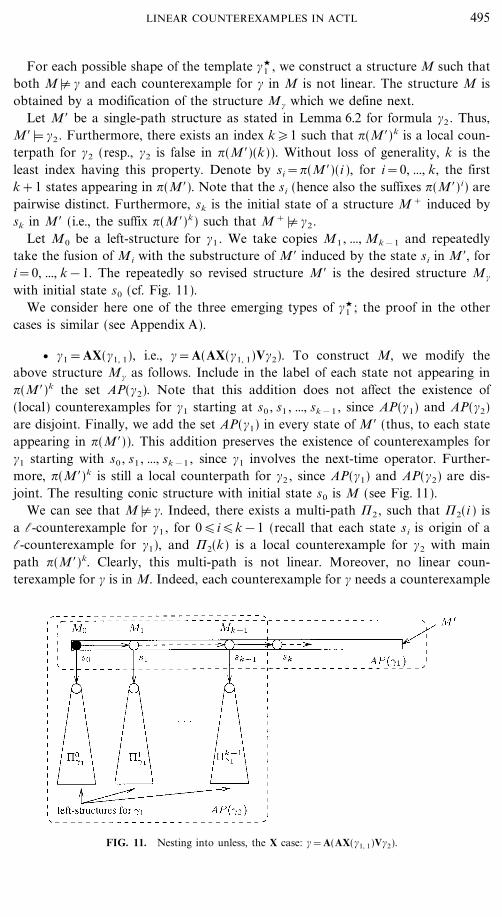
For each possible shape of the template #C1 , we construct a structure M such that

both M<% # and each counterexample for # in M is not linear. The structure M isobtained by a modification of the structure M# which we define next.

Let M$ be a single-path structure as stated in Lemma 6.2 for formula #2 . Thus,M$<#2 . Furthermore, there exists an index k�1 such that ?(M$)k is a local coun-terpath for #2 (resp., #2 is false in ?(M$)(k)). Without loss of generality, k is theleast index having this property. Denote by si=?(M$)(i ), for i=0, ..., k, the firstk+1 states appearing in ?(M$). Note that the si (hence also the suffixes ?(M$) i) arepairwise distinct. Furthermore, sk is the initial state of a structure M+ induced bysk in M$ (i.e., the suffix ?(M$)k) such that M +<% #2.

Let M0 be a left-structure for #1 . We take copies M1 , ..., Mk&1 and repeatedlytake the fusion of Mi with the substructure of M$ induced by the state si in M$, fori=0, ..., k&1. The repeatedly so revised structure M$ is the desired structure M#

with initial state s0 (cf. Fig. 11).We consider here one of the three emerging types of #C

1 ; the proof in the othercases is similar (see Appendix A).

v #1=AX(#1, 1), i.e., #=A(AX(#1, 1)V#2). To construct M, we modify theabove structure M# as follows. Include in the label of each state not appearing in?(M$)k the set AP(#2). Note that this addition does not affect the existence of(local) counterexamples for #1 starting at s0 , s1 , ..., sk&1 , since AP(#1) and AP(#2)are disjoint. Finally, we add the set AP(#1) in every state of M$ (thus, to each stateappearing in ?(M$)). This addition preserves the existence of counterexamples for#1 starting with s0 , s1 , ..., sk&1 , since #1 involves the next-time operator. Further-more, ?(M$)k is still a local counterpath for #2 , since AP(#1) and AP(#2) are dis-joint. The resulting conic structure with initial state s0 is M (see Fig. 11).

We can see that M<% #. Indeed, there exists a multi-path 62 , such that 62(i ) isa l-counterexample for #1 , for 0�i�k&1 (recall that each state si is origin of al-counterexample for #1), and 62(k) is a local counterexample for #2 with mainpath ?(M$)k. Clearly, this multi-path is not linear. Moreover, no linear coun-terexample for # is in M. Indeed, each counterexample for # needs a counterexample

FIG. 11. Nesting into unless, the X case: #=A(AX(#1, 1)V#2).


for #2 . But all paths starting with the initial state s0 cannot be a local counterpathfor #2 . Indeed, each path ? not reaching states beyond sk cannot be a counterpathfor #2 , since the label of each state appearing in ? would contain the set AP(#2). Onthe other hand, the only path starting with s0 and reaching sk is ?(M$). However,as M$ was chosen according to Lemma 6.2, this path cannot be a counterpath for#2 . Hence, we need a counterexample whose first element is a counterexample for#1 . Clearly, we cannot find a counterexample for #1 along the path ?(M$), sinceeach state in it contains AP(#1). Hence, each counterexample for # necessarily con-tains branching, that is, it is not linear.

This concludes the proof for the case in which #C1 , #C

2 have form A� or#C

2 # PSF. For the case of a general #C1 , Lemma 6.1 can be exploited: the instan-

tiation #1 is a monotone Boolean combination of positive disjoint instantiations#1, 1 , ..., #1, m (each of which occurs only once) such that w.l.o.g. #1, 1 is of the formA�. We proceed then for #1 as for #1, 1 , but use the structure M from Lemma 6.1for ,=#1 instead of the structure M+ for ,+=#1, 1 (observe that M+ can alwaysbe chosen such that R(M+) is total). For the general case of #2 , we proceedanalogously. This proves the result. K

Theorem 6.7. Let # be any positive disjoint instantiation of a template #C # TC.If #C � LIN, then # is not c-linear.

Proof. We proceed by induction on the number of universal quantifiers Aappearing in #, which is denoted by nA (#).

(Basis) The case nA (#)=0 is trivial, since #C belongs to PSF�LIN.

(Induction) Assume that the statement is true for every # such that nA (#)<k.We have to show that each positive disjoint instantiation # of #C # TC"LIN suchthat nA(#)=k is not c-linear, i.e., that there is a structure M such that both M<% #and each counterexample for # in M is not linear.

The formula # is either of the form A�, or a Boolean combination of formulas#1 , ..., #m . We consider the possible cases.

v #=AX,, where nA (,)=k&1. By Definition 4.9, #C � LIN if and only if,C � LIN. Thus, since nA (,)=k&1, the induction hypothesis implies that , is notc-linear. Hence, there exists a structure M$ such that both M$<% , and no coun-terexample for , in M$ is linear. Without loss of generality, M$ is conic and has theinitial state s$0 . Let the conic structure M with initial state s0 result by connectinga new state s0 to M$ via the transition (s0 , s$0 ). Clearly, M<% #. Furthermore, eachcounterexample 6 for # is such that 6(1) is a counterexample for ,. Sinceor(6(1))=s$0 , 6(1) cannot be linear, by hypothesis. Hence, 6 is not linear.

v #=A(#1V#2), where nA (#1)+nA (#2)=k&1. By the definition of LIN, thefollowing two cases cover each # such that #C � LIN:

1. #C1 � PSF and #C

2 # LIN. This case has been already proven inTheorem 6.6.

2. #C2 � LIN. By the induction hypothesis, #2 is not c-linear. Thus, there

exists a structure M such that M<% #2 and no counterexample in M is linear. We


modify M by adding in each state the set AP(#1). Clearly, no local counterexamplesfor #1 can be found in M. However, M<% #. Moreover, each counterexample for #in M must start with a counterexample for #2 . Hence, it is not linear.

v #=A(#1U#2), where nA (#1)+nA (#2)=k&1. Due to the intricatepossibilities of nesting into an until from LIN, this case requires a careful analysisof several subcases. The following cases exhaust each possibility of #C � LIN:

1. #C1 � PSF and #C

2 # LIN"PSF;

2. #C1 � LIN and #C

2 # PSF;

3. #C2 � LIN;

4. #C1 # PSF and #C

2 # LIN"(S �2 _ PSF ).

Case 1 is already proved by Theorem 6.6, and cases 2,3 are simple to prove fromthe induction hypothesis. For the remaining case 4, we conclude from Lemma 6.1that it is sufficient to consider the following cases for #C

2 , where ULIN=LIN &

AU(TC, TC) is the set of all linear until templates:

4.1. #C2 # AX(LIN).

4.2. #C2 # AV(PSF, LIN);

4.3. #C2 # ULIN 7 ULIN;

4.4. #C2 # (PSF 7 ULIN) _ (ULIN 7 PSF ).

Indeed, #2 is a positive disjoint instantiation of #C2 that can be viewed as monotone

Boolean combination of different atoms ,1 , ..., ,n where each ,i is either a purestate formula or of form A�. Since #C

2 � PSF, for some ,i either (i) ,i=AX�1 , (ii),i=A(�1V�2), or (iii) , i=A(�1U�2). If in case (iii) neither X nor V occur in #2 ,then some ,j where i{ j must exist such that ,C

j # PSF _ ULIN and the commonancestor of ,i and , j in the formula tree of #2 is a conjunction node (i.e., ,i and , j

are subformulas of formulas : and ;, respectively, such that : 7 ; is a subformulaof #2). Lemma 6.1 implies that it is sufficient to consider the formula ,+ where,+=,i in cases (i), (ii) and ,+=,i 7 ,j in case (iii). Indeed, no disjunction,+=,i 6 ,j needs to be considered: if no ,+ as in the cases (i)�(iii) exists, then,C

j # ULIN must hold for at least one ,j where j{i. (Otherwise, all ,j where j{iwould be pure state formulas and connected in #2 with disjunction. Thus, #C

2 # S �2

and #C # LIN would hold). However, disjunction of any two templates containingsubtemplates from ULIN clearly yields a template outside LIN, which would imply#C

2 � LIN. Now by Lemma 6.1, for any stucture M+ for ,+ such that R(M+) istotal and AP(M+) & AP(#2)=AP(,+), we can build a structure M for ,=#2 suchthat local counterpaths for ,+ in M+ coincide with local counterpaths for #2 in M.In particular, we obtain that if M+ has no counterpath for A(#1U,+), then M hasno counterpath for A(#1U#2).

We now describe structures for 4.1�4.4 proving the claim (see Appendix A fordetails).

4.1. #C2 # AX(LIN). Let M$ be a single-path structure and k�1 for for-

mula #2 as described in Lemma 6.2. Thus, M$<#2 , and ?(M$)k is a local counter-path for #2 (resp., M$, ?(M$)(k)<% #2). Let k w.l.o.g. be the least such index.


FIG. 12. Nesting of PSF and AX(TC) into until: #=A(#1 UAX(#2, 1)).

Let s0 , s1 , ..., sk denote the first k+1 states in ?(M$). These si are pairwise dis-tinct. Clearly, sk is the first state of the suffix ?(M$)k. We assume w.l.o.g.L(M$)(sk) & AP(#1)=<. Let M0 be a k-structure for #2 such that the initial statehas an empty label. Lemma 6.3 implies that such an M0 exists; observe thatM0<% #2 . Let M1 , ..., Mk&1 be copies of M0 . For i=0, ..., k&1 we repeatedly takethe fusion of Mi with the structure induced by si in M$. Finally, we add to everystate except sk the set AP(#1). The resulting structure is the desired M (see Fig. 12).

4.2. #C2 # AV(PSF, LIN). Thus, #2=A(#2, 1V#2, 2) , where #2, 1 is a pure

state formula and #2, 2 is c-linear by Theorem 5.1.Let M be a k-structure for #2 with initial state s$0 . Such a structure exists by

Lemma 6.3, and w.l.o.g. AP(M ) & AP(#1)=<. We modify M by adding a newinitial state s0 with empty label and the transitions (s0 , s$0 ) and (s0 , s0). Then, weadd to each state the set AP(#1) and to s0 the set AP(#2, 2) (see Fig. 13).

4.3. #C2 # ULIN 7 ULIN. Thus, #C

2 =,1 7 ,2 , where ,1=A(,1, 1U,1, 2) and,2=A(,2, 1U,2, 2) ; moreover, each ,i, j , i, j # [1, 2] is an instantiation of a tem-plate in LIN.

We construct M as follows. Let M$ be a single-path structure as in Lemma 6.2for formula ,2 . Thus, M$<,2 . Furthermore, there exists a k�1 such that ?(M$)k

is a local counterpath for ,2 (and hence for #2). Let k w.l.o.g. be the least suchindex. Let s0 , s1 , ..., sk , denote the first k+1 states appearing in ?(M$); observe thatthey are pairwise distinct. Clearly, sk is the first state of the suffix ?(M$)k. Since #is a positive disjoint instantiation, we may assume that no atom fromAP(#1) _ AP(,1) occurs in any state of M$.

Let M0 be a right-structure for ,1 ; since ,C1 # LIN, such a structure exists by

Lemma 6.4. We remark that, by definition of right-structure, M0<% ,1 . LetM1 , ..., Mk&1 be copies of M0 . For i=0, ..., k&1 we repeatedly take the fusion ofMi and the structure induced by the state si in M$. Next, we add in every state

FIG. 13. Nesting of PSF and AV(TC) into until: #=A(#1 UA(#2, 1V#2, 2)).


s0 , ..., sk&1 the set AP(,1, 1). Note that after this addition, each structure Mi stillsatisfies Mi <% ,1 , for i=1, ..., k&1. Indeed, since AP(,1, 1) & AP(,1, 2)=< for6 i

,1 , 2, still 6 i

,1 , 2<% ,1, 2 holds.

Now we add in every state of Mi , for 0�i�k&1, including states s0 , ..., sk&1 ,the set AP(#1). Since AP(#1) & AP(#2)=<, this has no effect on the properties ofMi from above. Moreover, we add in every state of Mi , for 0�i�k&1, exceptthe states s0 , ..., sk&1 , the set AP(,2). Since AP(,1) & AP(,2)=<, this additionpreserves the existence of counterexamples for ,1 in the Mi 's. Finally, we addAP(,1) in every state occurring in the path ?(M$)k. After this addition, ?(M$)k isstill a local counterpath for ,2 . The resulting structure is the desired M (seeFig. 14).

4.4. #C2 # (PSF 7 ULIN) _ (ULIN 7 PSF ). Thus, #2=,1 7 ,2 . Assume

that ,1 is a pure state formula and ,2=A(,2, 1U,2, 2) , where ,2, 1 and ,2, 2 areinstantiations of templates in LIN. The other case (vice versa) is similar.

Let M$ be a right-structure for ,2=A(,2, 1U,2, 2) . We modify M$ by addingAP(#1) _ AP(,1) to each state and by further adding AP(,2, 1) to s0; after thismodification M$<% ,2 still holds. We now add and label two new states s1 , s2 toobtain the desired M as shown in Fig. 15.

FIG. 14. Right-nesting of ULIN 7ULIN into until: #=A(#1U(,1 7 ,2)), where ,1=A(,1, 1U,1, 2)and ,2=A(,2, 1U,2, 2) .


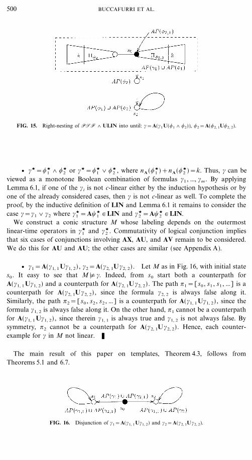
FIG. 15. Right-nesting of PSF 7 ULIN into until: #=A(#1U(,1 7 ,2)), ,2=A(,2, 1U,2, 2).

v #C=,C1 7 ,C

2 or #C=,C1 6 ,C

2 , where nA (,C1 )+nA (,C

2 )=k. Thus, # can beviewed as a monotone Boolean combination of formulas #1 , ..., #m . By applyingLemma 6.1, if one of the #i is not c-linear either by the induction hypothesis or byone of the already considered cases, then # is not c-linear as well. To complete theproof, by the inductive definition of LIN and Lemma 6.1 it remains to consider thecase #=#1 6 #2 where #C

1 =A�C1 # LIN and #C

2 =A�C2 # LIN.

We construct a conic structure M whose labeling depends on the outermostlinear-time operators in #C

1 and #C2 . Commutativity of logical conjunction implies

that six cases of conjunctions involving AX, AU, and AV remain to be considered.We do this for AU and AU; the other cases are similar (see Appendix A).

v #1=A(#1, 1U#1, 2) , #2=A(#2, 1U#2, 2) . Let M as in Fig. 16, with initial states0 . It easy to see that M<% #. Indeed, from s0 start both a counterpath forA(#1, 1U#1, 2) and a counterpath for A(#2, 1U#2, 2) . The path ?1=[s0 , s1 , s1 , ...] is acounterpath for A(#2, 1U#2, 2) , since the formula #2, 2 is always false along it.Similarly, the path ?2=[s0 , s2 , s2 , ...] is a counterpath for A(#1, 1U#1, 2) , since theformula #1, 2 is always false along it. On the other hand, ?1 cannot be a counterpathfor A(#1, 1U#1, 2) , since therein #1, 1 is always true and #1, 2 is not always false. Bysymmetry, ?2 cannot be a counterpath for A(#2, 1U#2, 2) . Hence, each counter-example for # in M not linear. K

The main result of this paper on templates, Theorem 4.3, follows fromTheorems 5.1 and 6.7.

FIG. 16. Disjunction of #1=A(#1, 1U#1, 2) and #2=A(#2, 1U#2, 2).


7. DISCUSSION AND CONCLUSION

For the class of ACTL formulas which are positive disjoint instantiations, theresults in the preceding sections give a complete characterization of the c-linearfragment. This class is given by those formulas # such that #C # LIN. Observe thatthis class is efficiently recognizable.

This result can be extended by the same proof technique to more general classesof formulas #, as long as certain independence properties hold on the pure state for-mulas. Introduce for each occurrence of a maximal pure state formula , in # a newpropositional atom p, , and consider the formula

F(#)= �, # MP(#)

( p, W ,),

where MP(#) is a list of all occurrences of maximal pure state formulas in #. Call# pure state independent, if for every truth value assignment to the atomic proposi-tions p, , the formula F(#) is satisfiable. Observe that every positive disjoint instan-tiation # is pure state independent.

Then, along the same line of proof as above we can show the following.

Theorem 7.1. Let # be any pure state independent formula. Then, # is c-linear ifand only if #C # LIN.

However, testing pure state independence is complex in general; this amounts toevaluating the quantified Boolean formula (QBF) 8=\P, _AP.F(#), where P, isthe collection of all atomic propositions p, introduced for occurrences of maximalpure state formulas, and AP is the collection of all atomic propositions in #. Thisproblem is complete for the class 6 p

2 of the polynomial hierarchy (cf. [8] for 6 p2 ).

Indeed, the evaluation of the QBFs \X _Y .� is in 6 p2 [8], and the QBF 8 is con-

structible in polynomial time from #. On the other hand, consider a QBF \X _Y.�,where � is of the form y1 7 �$ where y1 # Y. Then, the ACTL formula #=(AXx1) 7 } } } 7 (AXxn) 7 (AX�), where X=[x1 , ..., xn], is pure state independent,just if \X _Y.� is true. Since deciding the latter is 6 p

2 -hard, also deciding pure stateindependence is 6 p

2 -hard.Our results can be adapted for the concept of witness [5] in the existential frag-

ment of CTL (denote this by ECTL), i.e., a portion of a computation tree whichwitnesses the truth of a formula E,. Since on any structure M it holds that M<E,if and only if M<% Ac,, the existence of linear witnesses (formally defined in thesame vein as counterexamples) is related to the existence of linear counterexamples.As well-known [6], the equivalences cA(,V�)=E(c,Uc�) and cA(,U�)=E(c,Vc�) hold. It follows that a formula # in the existential CTL-fragment hasalways a linear witness (call this w-linear), if and only if the formula obtained bydualization of # and negating all elementary atomic propositions, is c-linear. As aconsequence, all instantiations of an ECTL-template #C (defined as obvious) havelinear witnesses (call this w-linear), just if the dual template d(#C) is c-linear. As aconsequence, we obtain the following characterization of the class of w-linearECTL-templates.


Theorem 7.2. Let #C be an ECTL-template. Then, #C is w-linear if and only ifd(#C) # LIN.

In this paper, we have considered Kripke structures M in which the transitionrelation R(M) is arbitrary. As already pointed out, many authors (e.g. [7, 10])require that R(M ) is total. It appears that our main results (precisely,Theorems 4.1�4.3, 5.2, 5.3) and in particular Theorem 6.7 remain valid underrestriction to the class of structures that have total transition relations. The struc-ture M in the proof of Theorem 4.1 has total R(M) by construction, and totalityof R(M) can be assumed to hold for M in the proof of Theorem 4.2 without lossof generality, since a graph having a node with no outgoing edges trivially has noHamiltonian cycle. Furthermore, all structures in the proof of Theorem 6.7 that wehave constructed for proving that certain formulas are not c-linear have total R(M)if their constituents have.

Several issues remain for further work. One issue is the consideration of lineartime operators which are derived from the basic operators X, V, U. The mostimportant such operators are F (sometimes) and G (globally, always) defined asF,=trueU,, G,= falseV,. It is easily recognized from the definition of LIN andour results that these operators correspond to c-linear templates. However, the useof these templates in nesting, as well as the use of true and false in general, appearsto be nontrivial. The characterization of the class of c-linear templates ACTLenriched by derived linear time operators and�or constants true and false is aninteresting issue which remains to be explored.

Finally, an extension of our study by fairness constraints [4] would be interest-ing. In the general framework, path quantifiers do not range over all infinite paths,but instead over paths along which the fairness constraints, expressed by formulas,must be satisfied infinitely often. E.g., fair schedules in a system of concurrentinfinite processes, represented through a Kripke structure, can be expressed easilythrough fairness constraints. Our results do not immediately carry over to this case.Techniques applied in [5, 9] might be useful.

APPENDIX: PROOFS

Lemma 6.2. For every positive disjoint instantiation # of a template #C # LIN,there exists a single-path structure M and a k�1 such that M<# and ?(M)k is alocal counterpath for # (resp., ?(M)(k)<% # if #C # PSF).

Proof. We prove the statement by induction on the stage i�0 of 4i=(S i1 , S i

2)in which #C first occurs.

(Basis) The case i=0 is trivial.

(Induction) Assume that the statement holds for i and consider the possiblecases for #C # S i+1

1 _ S i+12 where i+1>0. By the induction hypothesis, it remains

to consider #C � S i1 _ S i

2 .

v #C # PSF. (In this case, i=1.) Let M have the states s0 and s1 , where s0

is the unique initial state, and the transitions (s0 , s1), (s1 , s1). Let L(M)(s0)=AP(#)


and L(M )(s1)=<. Clearly, M is a single-path structure such that M<#, andM, ?(M )1(0)<% #. Thus the statement holds.

v #C # AX(S i1). Thus, #=AX(#1). By the induction hypothesis, a single-path

structure M with initial state s0 and a k�1 exist for #1 which satisfy the statementof the lemma. Let k* be the least such k. If k*>1 we are done, since M is a single-path structure where also # satisfies the statement of the lemma. Otherwise (i.e., ifk*=1), we can modify M by adding a new state s$0 which reaches s0 and has anarbitrary label. Denote by M$ the resulting single-path structure with initial state s$0 .Since ?(M$)1=?(M ), it holds that M$<#. Furthermore, ?(M$)1 is a local counter-path for #, since ?(M$)2=?(M )1. Hence the statement holds.

v #C # AV(PSF, S i1). Let #=A(#1V#2). By induction hypothesis, for #2

exist a single-path structure M and an index k�1 such that the property of thelemma holds. We modify M by adding AP(#1) to every state label in M. It is easyto see that the resulting structure M$ satisfies M$<# because #1 is globally truealong ?(M$). Furthermore, ?(M$)k is still a local counterpath for #2 (resp.,?(M$)(k)<% #2) since # is a disjoint positive instantiation. Hence, the statementholds.

v #C # AU(S i1 , PSF ). Thus, #=A(#1U#2). Consider the single-path struc-

ture M with states s0 and s1 , where s0 is the initial state, transitions (s0 , s1), (s1 , s1)and labeling L(M )(s0)=AP(#2) and L(M )(s1)=<. This M and k=1 prove thestatement for #. Indeed, M<# since #2 is true in s0 . Further, ?(M)1 is a local coun-terpath for # since #2 is globally false along it.

v #C # AU(PSF, S i2). Thus, #=A(#1 U#2). By induction hypothesis, for #2

exist a single-path structure M and an index k�1 as in the lemma. Without lossof generality, no atomic proposition from AP(#1) occurs in any state label of M.Since # is a positive disjoint instantiation, it is easy to see that M and k witness thestatement also for #. Indeed, M<# since #2 is true in the initial state of M. Further-more, ?(M )k is a local counterpath for #, since it is a local counterpath for #2 (resp.,#2 is false in ?(M)(k)) and #1 is globally false along it.


1 . Thus, #=#1 6 #2 . Assume that #C1 �

PSF; the case #C2 � PSF is similar. By induction hypothesis, for #1 exist a single-

path structure M and an index k�1 as stated in the lemma. Without loss ofgenerality, no atomic proposition from AP(#2) occurs in any state label of M. Since# is a positive disjoint instantiation, it is easy to see that M and k witness the state-ment also for #. Indeed, M<# since M<#1 . Further, ?(M )k is a local counterpathfor # since it is a local counterpath for #1 (resp., #1 is false in ?(M )(k)) and #2 isglobally false along it. Thus, the statement holds.

v #C # S i1 7 S i

1 . Thus, #=#1 7 #2 , and w.l.o.g. #C1 � PSF. By induction

hypothesis, for #1 exist a single-path structure M and an index k�1 as stated in thelemma. We modify M by adding to every state label the set of atomic propositionsappearing in #2 . It is easy to see that the resulting structure M$ and k witness thestatement also for #. Clearly, M$<# since M$<#1 and M$<#2 since #2 is globallytrue in M$. Furthermore, ?(M$)k is a local counterpath for # since it is a local coun-terpath for #1 . Thus, the statement holds. This concludes the proof. K


Lemma 6.3. Each positive disjoint instantiation # of any template #C # LIN hassome single-path k-structure M.


2) in which #C first occurs.

(Basis) The case i=0 is trivial.

(Induction) Assume that the statement holds for i, and consider the possiblecases for #C # S i+1

1 _ S i+12 , where i+1>0. By the induction hypothesis, it remains

to consider #C � S i1 _ S i

2 .

v #C # PSF. (In this case, i=1.) Let M have the states s0 and s1 , where s0

is the unique initial state, and the transitions (s0 , s1), (s1 , s1). Let L(M )(s0)=<and L(M )(s1)=AP(#). Clearly, M is a single path structure such that M<% #, andM, ?(M )1(0)<#. Thus the statement holds.

v #C # AX(S i1). Let #=AX(#1). By induction hypothesis, there exist a single-

path structure M and an index k�1 such that M<% #1 and M, ?(M ) i (0)<#1 for alli�k. Let s0 be the initial state of M. We modify M by changing the initial state toa new state s with arbitrary label and adding the transition (s, s0). Clearly, theresulting structure M$ is single-path and M$<% #. From the induction hypothesis, itfollows that for each i�k+1, M$, ?(M$) i (0)<#1 . Hence, the statement holds.

v #C # AV(PSF, S i1). Let #=A(#1V#2). Let s0 be the initial state of a single-

path structure M for #2 and k�1 as stated in the lemma, which exist by the induc-tion hypothesis. Since M<% #2 , it follows M<% #. Furthermore, M, +(6 ) i (0)<#2

implies M, +(6 ) i (0)<#, for each i�k. Thus the statement holds.

v #C # AU(S i1 , PSF ). Let #=A(#1 U#2). Let for #1 be M and k�1 as

stated in the lemma, which exist by induction hypothesis. Without loss ofgenerality, M includes AP(#2) in each state label L(s) except for the initial state s0 ,which contains no atomic proposition from AP(#2). Then, M, s0 <% #2 , and sinceM<% #1 , it follows M<% #. Furthermore, M, ?(M ) i (0)<# for all i�k since #2 is truein ?(M) i (0). Thus, the statement holds.

v #C # AU(PSF, S i2). Let #=A(#1U#2). Let for #2 be M and k�1 as stated

in the lemma, whose existence follows from the induction hypothesis. Without lossof generality, we assume that the initial state s0 of M contains no atomic proposi-tion from AP(#1). Since M<#2 , it follows M<% #. Furthermore, since M, ?(M ) i

(0)<#2 it follows that M, ?(M ) i (0)<#, for all i�k. Thus the statement holds.


1 . Let #=#1 6 #2 . Assume #C1 � PSF; the

case #C2 � PSF is similar. Let for #1 be M and k�1 as stated in lemma, which

exist by induction hypothesis. Assume without loss of generality that no atomicproposition from AP(#2) occurs in any label of M. Then, it is easy to see that Mand k witness the statement for #.

v #C # S i1 7 S i

1 . Let #=#1 7 #2 . Let for #1 be M and k�1 as stated in thelemma, which exist by the induction hypothesis. Assume without loss of generalitythat #C

1 � PSF, and that each label of M includes AP(#2). Since #2 is globally truein M, it is easy to see that M and k witness the statement also for #. This concludesthe proof. K


Theorem 6.6. Let # be a positive disjoint instantiation of a template #C # TC suchthat either

1. #=A(#1U#2), where #C1 � PSF and #C

2 # LINnPSF, or

2. #=A(#1V#2), where #C1 � PSF and #C

2 # LIN.

Then, # is not c-linear.

Proof. (1) The following six cases remain.

v #1=AX(#1, 1) and #2=A(#2, 1V#2, 2) . We modify M in the following way.We add to every state s of M1 except s0 the set AP(#2). Similarly, we add to everystate of M2 except s0 the set AP(#1). Finally, we add in every other state of 6#2 , 1

in M2 (see definition of right-structure), including s0 , the set AP(#2, 2) (see Fig. 17).It easy to see that after these additions, M1<% #1 and M2<% #2 still hold. Thus,

M<% #. Moreover, no counterexample for #1 is in M2 . Indeed, for every multi-path6 in M2 , 6(1) cannot be a counterexample for #1, 1 , since each state of M2 exceptcontains the set AP(#1, 1). Finally, no counterexample for #2 is in M1 . Indeed, acounterexample for #2 must contain a counterexample for #2, 2. However, this isimpossible, since #2, 2 is globally true in M1 . Hence, a counterexample for # involv-ing counterexamples for both #1 and #2 cannot be linear. By Definition 3.5 a coun-terexample for # must involve counterexamples for #2 . Now we show that everycounterexample for # involving only counterexamples for #2 is not linear. Clearly,this concludes the proof. Towards a contradiction, suppose 6 is a linear coun-terexample involving only counterexamples for #2 . By Definition 3.5, 6 is such that6(i ) is a counterexample for #2 , for each i�0. But such a counterexample cannotbe linear. Indeed, 6 cannot lead into 6#2

, since it is a k-structure of #2 . On theother hand, it cannot lead into M1 or 6#2 , 1

, since a counterexample for #2 mustcontain a counterexample for #2, 2 , and #2, 2 is globally true in 6#2 , 1

. Hence, everycounterexample for # in M is not linear.

v #1=AX(#1, 1) and #2=A(#2, 1U#2, 2) . We modify M as follows. We add toevery state of M1 except s0 the set AP(#2), and to every state of M2 except s0 the

FIG. 17. The X-V case: A(#1 U#2), where #1=AX(#1, 1) and #2=A(#2, 1V#2, 2).


FIG. 18. The X-U case: A(#1U#2), where #1=AX(#1, 1) and #2=A(#2, 1U#2, 2).

set AP(#1). Finally, we add in every state of 6#2 , 2in M2 including s0 the set

AP(#2, 1) (see Fig. 18).It easy to see that after these additions M1<% #1 and M2<% #2 still hold. Thus,

M<% #. Moreover, no counterexample for #1 is in M2 . Indeed, for every multi-path6 in M2 , 6(1) cannot be a counterexample for #1, 1 , since each state of M2 excepts0 contains the set AP(#1, 1). Finally, no counterexample for #2 is in M1 . Indeed,since each state of M1 contains AP(#2, 1) , a counterexample for #2 in M1 could onlybe a multi-path 6 such that 6(i ) is a counterexample for #2, 2, for each i�0.But this is impossible, since for every multi-path 6 in M1 , each state appearingin 6(i ), for i�1 contains AP(#2, 2) . Hence, a counterexample for # involving coun-terexamples for both #1 and #2 cannot be linear. Definition 3.5 requestthat a counterexample for # must involve a counterexample for #2 . Now we showthat every counterexample for # involving only counterexamples for #2 is not linear.This, clearly, concludes the proof. Towards a contradiction, suppose 6 is alinear counterexample for # such that 6(i ) is a counterexample for #2 , for everyi�0. But such a counterexample cannot be linear. Indeed, it can neither lead intoM1 nor into 6#2

, since this is a k-structure of #2 . Furthermore, it cannot lead into6#2 , 2

. Indeed, a counterexample for #2 cannot involve a counterexample for #2, 1

as 6#2 , 2contains in each state the set AP(#2, 1) . Thus, such a counterexample

could only be a multi-path 6 such that 6(i ) is a (linear) counterexample for #2, 2,for each i�0. But this is not possible, since 6#2 , 2

is a k-structure of #2, 2 . Hence,no counterexample for # in M is linear.

v #1=A(#1, 1V#1, 2) and #2=AX(#2, 1) . We modify M as follows. We add toevery state of M1 except s0 the set AP(#2) and to every state of M2 except s0 theset AP(#1). Moreover, we add to s0 the set AP(#1, 2) . Finally, we add in every otherstate of 6#1 , 1

in M1 (see definition of left-structure), the set AP(#1, 2) (see Fig. 19).After these additions, M1<% #1 and M2<% #2 still hold. Thus, M<% #. Moreover, no

counterexample for #2 is in M1 . Indeed, for every multi-path 6 in M1 , 6(1) cannotbe a counterexample for #2, 1, since each state of M1 except s0 contains the setAP(#2, 1) . Finally, no counterexample for #1 is in M2 . Indeed, a counterexample for


FIG. 19. The V-X case: A(#1 U#2), where #1=A(#1, 1V#1, 2) and #2=AX(#2, 1).

#1 must contain a counterexample for #1, 2 , but this is impossible, since each statein M2 contains AP(#1, 2) . Hence, a counterexample for # involving counterexamplesfor both #1 and #2 cannot be linear. By Definition 3.5, a counterexample for # mustinvolve counterexamples for #2 . Now we show that every counterexample for #involving only counterexamples for #2 is not linear. This, clearly, concludes theproof. Towards a contradiction, suppose 6 is a linear counterexample involvingonly counterexamples for #2 . Definition 3.5 implies that 6(i ) is a counterexamplefor #2 , for each i�0. But such a counterexample cannot be linear. Indeed, 6 cannotlead into M1 and not into M2 , since 6#2 , 1

is a k-structure of #2, 1. This proves thestatement.

v #1=A(#1, 1V#1, 2) and #2=A(#2, 1V#2, 2) . We modify M as follows. We addto every state of M1 except s0 the set AP(#2). Then, we add to every state of M2

except s0 the set AP(#1). Moreover, we add to s0 the set AP(#1, 2) . Finally, we addin every state of 6#2 , 1

in M2 , including s0 , the set AP(#2, 2) (see Fig. 20).

FIG. 20. The V-V case: A(#1 U#2), where #1=A(#1, 1V#1, 2) and #2=A(#2, 1V#2, 2).


FIG. 21. The U-X case: A(#1U#2), where #1=A(#1, 1U#1, 2) and #2=AX(#2, 1).

It easy to see that, also after these additions, M1<% #1 and M2<% #2 . Thus, M<% #.Moreover, no counterexample for #1 is in M2 . Indeed, #1, 2 is globally true in M2 .Similarly, no counterexample for #2 is in M1 . Hence, a counterexample for # involv-ing counterexamples for both #1 and #2 cannot be linear.

By Definition 3.5, a counterexample for # must involve a counterexample for #2 .Now we show that every counterexample for # involving only counterexamples for#2 is not linear. This, clearly, concludes the proof. Towards a contradiction, suppose6 is a linear counterexample for #2 such that 6(i ) is a counterexample for #2 , foreach i�0. But such a counterexample cannot be linear. Indeed, 6 cannot lead intoM1 , and it cannot lead into 6#2

since it is a k-structure of #2 . On the other hand,it cannot lead into 6#2 , 1

, since a counterexample for #2 must contain a coun-terexample for #2, 2 and #2, 2 is globally true in 6#2 , 1

. Hence, every counterexamplefor # in M is not linear.

v #1=A(#1, 1U#1, 2) and #2=AX(#2, 1) . We modify M in the following way.We add to every state of M1 except s0 the set AP(#2) and to every state of M2

except s0 the set AP(#1). Finally, we add in every state of 6#1 , 2in M1 the set

AP(#1, 1) (see Fig. 21).It easy to see that, also after these additions, M1<% #1 and M2<% #2 . Thus, M<% #.

Moreover, no counterexample for #2 is in M1 . Indeed, for every multi-path 6 inM1 , 6(1) cannot be a counterexample for #2, 1, since each state of M1 except s0 con-tains the set AP(#2, 1) . Finally, no counterexample for #1 is in M2 . Indeed, sinceeach state of M2 contains the set AP(#1, 1), a counterexample for #1 in M2 couldonly be a multi-path 6 such that each element 6(i ) is a counterexample for #1, 2 ,for each i�0. But this is impossible, since for every multi-path 6 in M2 , each stateappearing in 6(i ) contains the set AP(#1, 2) , for each i�1. Hence, a counterexam-ple for # involving counterexamples for both #1 and #2 cannot be linear. By Defini-tion 3.5 a counterexample for # must involve a counterexample for #2 . Now weshow that every counterexample for # involving only counterexamples for #2 is notlinear. This, clearly, concludes the proof. Towards a contradiction, suppose 6 is alinear counterexample such that 6(i ) is a counterexample for #2 , for each i�0. Butsuch a counterexample cannot be linear. Indeed, 6 cannot lead into M1 , since #2

is globally true in M1 , and it cannot lead into M2 , since 6#2 , 1is a k-structure of

#2, 1. Thus, the statement is proven.


FIG. 22. The U-V case: A(#1U#2), where #1=A(#1, 1U#1, 2) and #2=A(#2, 1V#2, 2).

v #1=A(#1, 1U#1, 2) and #2=A(#2, 1V#2, 2) . We modify M in the followingway. We add to every state of M1 except s0 the set AP(#2). Then, we add to everystate of M2 except s0 the set AP(#1). Moreover, we add to s0 the set AP(#1, 1) _

AP(#2, 2) . Finally, we add to every other state of 6#2 , 1in M2 the set AP(#2, 2) (see

Fig. 22).It easy to see that after these additions, M1<% #1 and M2<% #2 hold. Thus, M<% #.

Moreover, no counterexample for #1 is in M2 . Indeed, #1, 1 is globally true in M2

and for every multi-path 6 in M2 , 6(i ), for i�1, cannot be a counterexample for#1, 2 , since each state of M2 except s0 contains the set AP(#1, 2) . Finally, no coun-terexample for #2 is in M1 . Indeed, #2, 2 is globally true in M1 . Hence, a coun-terexample for # involving counterexamples for both #1 and #2 cannot be linear. ByDefinition 3.5, a counterexample for # must involve a counterexample for #2 . Nowwe show that every counterexample for # involving only counterexamples for #2 isnot linear. This, clearly, concludes the proof. Towards a contradiction, suppose 6is a linear counterexample for # such that 6(i ) is a counterexample for #2 , for eachi�0. Such a counterexample cannot be linear. Indeed, 6 can neither lead into M1

(cf. above) nor into 6#2 , 1, since a counterexample for #2 must contain a coun-

terexample for #2, 2 which is globally true in 6#2 , 1. Furthermore, 6 cannot lead into

6#2, since it is a k-structure of #2 . Hence, no counterexample for # in M is linear.

v #1=A(#1, 1U#1, 2) and #2=A(#2, 1U#2, 2) . We modify M in the followingway. We add to every state of M1 except s0 the set AP(#2) and to every state of M2

except s0 the set AP(#1). Moreover, we add in s0 the set AP(#1, 1) _ AP(#2, 1) .Finally, we add in every other state of 6#2 , 2

in M2 (see definition of right-structure)the set AP(#2, 1) (see Fig. 23).

It easy to see that after these additions, M1<% #1 and M2<% #2 hold. Thus, M<% #.Moreover, no counterexample for #1 is in M2 . Indeed, #1, 1 is globally true in M2

and for every multi-path 6 in M2 , 6(i ), for i�1, cannot be a counterexample for


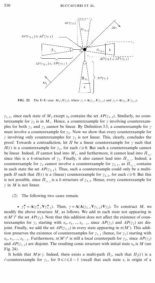
FIG. 23. The U-U case: A(#1U#2), where #1=A(#1, 1U#1, 2) and #2=A(#2, 1U#2, 2).

#1, 2 , since each state of M2 except s0 contains the set AP(#1, 2) . Similarly, no coun-terexample for #2 is in M1 . Hence, a counterexample for # involving counterexam-ples for both #1 and #2 cannot be linear. By Definition 3.5, a counterexample for #must involve a counterexample for #2 . Now we show that every counterexample for# involving only counterexamples for #2 is not linear. This, clearly, concludes theproof. Towards a contradiction, let 6 be a linear counterexample for # such that6(i ) is a counterexample for #2 , for each i�0. But such a counterexample cannotbe linear. Indeed, 6 cannot lead into M1 , and furthermore, it cannot lead into 6#2

,since this is a k-structure of #2 . Finally, it also cannot lead into 6#2 , 2

. Indeed, acounterexample for #2 cannot involve a counterexample for #2, 1 , as 6#2 , 2

containsin each state the set AP(#2, 1) . Thus, such a counterexample could only be a multi-path 6 such that 6(i ) is a (linear) counterexample for #2, 2 , for each i�0. But thisis not possible, since 6#2 , 2

is a k-structure of #2, 2. Hence, every counterexample for# in M is not linear.

(2) The following two cases remain.

v #C1 =A(#C

1, 1V#C1, 2) . Then, #=A(A(#1, 1 V#1, 2)V#2). To construct M, we

modify the above structure M# as follows. We add in each state not appearing in?(M$)k the set AP(#2). Note that this addition does not affect the existence of coun-terexamples for #1 starting with s0 , s1 , ..., sk&1 , since AP(#1) and AP(#2) are dis-joint. Finally, we add the set AP(#1, 2) in every state appearing in ?(M$). This addi-tion preserves the existence of counterexamples for #1, 1 (hence, for #1) starting withs0 , s1 , ..., sk&1. Furthermore, ?(M$)k is still a local counterpath for #2 , since AP(#2)and AP(#1, 2) are disjoint. The resulting conic structure with initial state s0 is M (seeFig. 24).

It holds that M<% #. Indeed, there exists a multi-path 62 , such that 62(i ) is al-counterexample for #1 , for 0�i�k&1 (recall that each state si is origin of a


FIG. 24. Nesting into unless, the V case: #=A(A(#1, 1V#1, 2)V#2).

l-counterexample for #1), and 62(k) is a local counterexample for #2 with mainpath ?(M$)k. Clearly, this multi-path is not linear. Moreover, no linear coun-terexample for # in M exists. Indeed, each counterexample for # needs a coun-terexample for #2 . It holds that every path starting at s0 cannot be a counterpathfor #2 . Indeed, each path ? not reaching the state sk cannot be a counterpath for#2 , since the label of each state appearing in ? would contain the set AP(#2).

On the other hand, the only path starting at s0 and reaching sk is ?(M$). As M$was chosen according to Lemma 6.2, this path cannot be a counterpath for #2 byconstruction. Hence, we need a counterexample such that the first element is acounterexample for #1 . Clearly, we cannot find a counterexample for #1 along thepath ?(M$), since each state in it contains AP(#1, 2) (and a counterexample for #1

necessarily contains a counterexample for #1, 2) . Hence, each counterexample for #necessarily contains branching, that is, it is not linear.

v #1=A(#1, 1U#1, 2) , i.e., #=A(A(#1, 1U#1, 2)V#2). We modify the structureM# from above as follows. We add to each state not appearing in ?(M$)k the setAP(#2). Note that this addition does not affect the existence of local counter-examples for #1 starting at s0 , s1 , ..., sk&1 , since AP(#1) and AP(#2) are disjoint.Furthermore, add the set AP(#1, 1) in every state appearing in ?(M$). This additionpreserves the existence of counterexamples for #1, 2 (hence for #1) starting at


s0 , s1 , ..., sk&1. Finally, we add in every state appearing in ?(M)k the set AP(#1, 2) .Clearly, after this addition ?(M$)k is still a local counterpath for #2 , since AP(#1)and AP(#2) are disjoint. The resulting conic structure with initial state s0 is M (seeFig. 25).

We can see that M<% #. Indeed, there exists a multi-path 62 , such that 62(i ) isa l-counterexample for #1 , for 0�i�k&1, and 62(k) is a counterexample for #2

with main path ?(M$)k. Clearly, this multi-path is not linear. Moreover, no linearcounterexample for # exists in M. Indeed, each counterexample for # needs a coun-terexample for #2 . Every path ? starting at the initial state s0 cannot be a counter-path for #2 . Indeed, if ? does not reach the state sk , it cannot be a counterpath for#2 , since the label of each state appearing in ? would contain the set AP(#2). Onthe other hand, the only path starting at s0 and reaching sk is ?(M$)k. Since M$ waschosen according to Lemma 6.2, it is not a counterpath for #2 . Hence, we need acounterexample whose first element is a counterexample for #1 . Clearly, we cannotfind a counterexample for #1, 1 along the path ?(M$), since each state in it containsthe set AP(#1, 1). Hence, a counterexample for #1 could only be a multi-path 6 suchthat 6(i ) is a counterexample for #1, 2, for each i�0. But such a counterexamplecannot be found along the path ?(M$). Indeed, along its suffix ?(M$)k the formula#1, 2 is always true.

Hence, each counterexample for # necessarily contains branching, that is, it is notlinear. K

FIG. 25. Nesting into unless, the U case: #=A(A(#1, 1U#1, 2)V#2).


Theorem 6.7. Let # be any positive disjoint instantiation of a template #C # TC.If #C � LIN, then # is not c-linear.

Proof (continued).

v #=A(#1U#2), where nA (#1)+nA (#2)=k&1.

2. #C1 � LIN and #C

2 # PPSF. Since #C1 � LIN, by the induction hypoth-

esis a structure M exists such that M<% #1 and no counterexample for #1 in Mis linear. Without loss of generality, M is conic with initial state s0 andAP(#2) & AP(M )=<.

Clearly, M<% #, since M<% #2 . Modify now M by adding to each state except s0

the set AP(#2). Since AP(#1) & AP(#2)=<, still M<% #1 holds. Moreover, sinceL(M )(s0) & AP(#2)=<, also M<% #2 holds. Thus, M<% #. It holds that each coun-terexample for # in M must contain a counterexample for #1 , and thus it is notlinear. Indeed, in any alternative counterexample 6 for # the element 6(i ) woulda local counterexample for #2 , for every i�0. Since all states of M except s0 containAP(#2), this is impossible.

3. #C2 � LIN. By the inductive hypothesis, there exists a structure M such

that both M<% #2 and each counterexample for #2 in M is not linear. W.l.o.g., M isconic with initial state s0 and AP(#1) & AP(M)=<.

Clearly, M<% #, where #=A(#1U#2), since M<% #1 and M<% #2 . We can concludethat each counterexample for # in M is not linear. Indeed, if 6 is a counterexamplefor # in M, 6(0) must be a l-counterexample for #2 . Moreover or(6(0))=s0 .Hence, 6(0) is a counterexample for #2 in M. Consequently, 6(0) and hence also6 cannot be linear.

4.1. First observe that M<% #. Indeed, each state si , for 0�i�k is origin ofa local counterexample for #2 . Furthermore, sk is also origin of a local coun-terexample for #1 . It remains to show that no linear counterexample is in M. In anycounterexample 6 for # the element 6(0) must be a counterexample for #2 . Thisimplies that a counterpath for # cannot reach state sk . Indeed, the only path reach-ing state sk is ?(M$), which by construction is not a counterpath for #2 . Thus, acounterpath ? for # could only lead into some structure Mi , where 0�i�k&1.However, in each Mi formula #1 is globally true. Hence ? would have to satisfy that? j, for each j�1, is a local counterpath for #2 . Since each Mi is a k-structure for#2 , this is impossible. This proves that no linear counterexample for # exists in M.

4.2. The path [s0 , s$0 , ...] is a counterpath for #2 . Thus, the multi-path[[s0 , s$0 , ...], [s0 , s$0 ...], ...] is a counterexample for the #. It holds that no linearcounterexample for # exists in M. Indeed, since AP(#1) is contained in eachstate, any counterexample for # must contain infinitely many counterexamplesfor #2 . Since s$0 is the initial state of a k-structure for #2 , no counterpath for # ispossible which reaches s$0 . Hence, the only possibility for a counterpath of # is?=[s0 , s0 , s0 , ...]. Since s0 contains AP(#2, 2) , this is impossible. Thus, non linearcounterexample for # exists.

4.3. First observe that M<% #. Indeed, each state si , for 0�i�k&1 is originof a local counterexample for ,1 and thus for #2 . Furthermore, sk is also origin ofa local counterexample for ,2 , and then for #2 . Moreover, sk is a local coun-terexample for the formula #1 .


Now we show that no linear counterexample for # exists in M. By Definition 3.5,in any counterexample 6 for # the element 6(0) must be a counterexample for #2 .Hence, a counterpath for # cannot reach state sk . Indeed, the only path reachingstate sk is ?(M$). This path is not a counterpath for #2 by construction: 6(M$) doesnot contain any local counterpath for ,1 , and, moreover, ?(M$) is not an counter-path for ,2 . Thus, a counterpath ? for # could only lead into some structure Mi ,where 0�i�k&1. Since in each Mi formula #1 is globally true, the suffix ?i mustbe a local counterpath for #2 , for each i�1. Since each state in Mi except the initialstate si contains AP(,2), this counterpath for #2 can only be a counterpath for ,1 .But this is impossible, since a right-structure for formula ,1 cannot contain a linearcounterexample 6 such that 6(i ) is a counterexample for ,1 , for each i�0. Thus,it follows that no linear counterexample for # exists in M.

4.4. It holds that M<% #. Indeed, there exists a counterexample 6 for #where 6(0) is a counterexample for #2 , and 6(1) is a counterexample for both #1

and #2 . Furthermore, no linear counterexample for # exists in M. To see this,observe that no path ? leading into 6,2

or into 6,2 , 2can be a counterpath for #,

as #1 and ,1 are always true there and 6,2, 6,2 , 2

are k-structures for ,2, 2 (conse-quently, ,2 is not globally false). Thus, only ?=[s0 , s1 , s2 , s2 , ...] remains as acandidate for a counterpath for #. To eliminate ?, assume towards a contradictionthat ?=+(6 ) for some linear counterexample 6 for #. The first element 6(0) ofevery counterexample 6 for # must be a counterexample for #2=,1 7 ,2 ; since ,1

is true in s0 , it must be a counterexample of ,2 . Along ?, however, ,2, 2 is notalways false, which means that 6(0) must involve a counterexample for ,2, 1. Along?, however, ,2, 1 is by construction always true. This raises a contradiction, andproves that in M no linear counterexample for # exists.

v #C=,C1 7 ,C

2 or #C=,C1 6 ,C

2 , where nA (,C1 )+nA (,C

2 )=k. In the remain-ing five cases, the labeling of M is chosen as follows (the suitability of M is easilyverified):

v #1=A(#1, 1U#1, 2) , #2=A(#2, 1V#2, 2) . Set L(M )(s0)=AP(#1, 1) _ AP(#2, 2) ,L(M )(s1)=AP(#1), and L(M)(s2)=AP(#1, 1) _ AP(#2, 2) .

v #1=A(#1, 1V#1, 2) , #2=A(#2, 1V#2, 2) . Set L(M )(s0)=AP(#1, 2) _ AP(#2, 2) ,L(M )(s1)=AP(#1, 2) , and L(M )(s2)=AP(#2, 2) .

v #1=AX(#1, 1), #2=AX(#2, 1) . Set L(M)(s0)=<, L(M )(s1)=AP(#1, 1), andL(M )(s2)=AP(#2, 1) .

v #1=AX(#1, 1), #2=A(#2, 1U#2, 2) . Set L(M)(s0)=AP(#2, 1) , L(M)(s1)=AP(#1), and L(M)(s2)=AP(#2).

v #1=AX(#1, 1), #2=A(#2, 1V#2, 2) . Set L(M)(s0)=AP(#2, 2) , L(M)(s1)=AP(#1, 1), and L(M)(s2)=AP(#2, 2) .

ACKNOWLEDGMENTS

We thank the reviewers for their detailed and constructive comments which helped to improve thispaper. This work has been partially supported by the Austrian Science Fund under Project N Z29-INF.Part of the work of Nicola Leone was done while he was with the Institut fu� r Informationssysteme,Technische Universita� t Wien.


REFERENCES

1. F. Buccafurri, T. Eiter, G. Gottlob, and N. Leone, Enhancing model checking in verification by AItechniques, Artificial Intelligence 112 (1999), 57�104.

2. E. Clarke and E. Emerson, Skeletons for branching time temporal logic, in ``Logic in Programs:Workshop Proceedings,'' Lecture Notes in Computer Science, Vol. 131, Springer-Verlag, Berlin�NewYork, 1981.

3. E. Clarke, E. Emerson, and A. Sistla, Automatic verification of finite-state concurrent systems usingtemporal logic specifications, ACM Trans. Programming Languages 8 (1996), 244�263.

4. E. Clarke, O. Grumberg, and D. Long, Verification tools for finite-state concurrent systems, in`À Decade of Concurrency��Reflections and Perspectives'' (J. de Bakker, W. de Roever, andG. Rozenberg, Eds.), Lecture Notes in Computer Science, Vol. 803, pp. 124�175, Springer-Verlag,Berlin�New York, 1994.

5. E. Clarke, O. Grumberg, K. McMillan, and K. Zhao, Efficient generation of counterexamples andwitnesses in symbolic model checking, in ``Proc. 32nd ACM�SIGDA Design Automation Conference1995 (DAC '95),'' ACM Press, New York, 1994. [Also Technical Report CMU-CS-94-204, CarnegieMellon University, Pittsburgh, PA, 1994.]

6. E. Clarke, O. Grumberg, and D. Long, Model checking, in ``Deductive Program Design'' (M. Broy,Ed.), Vol. 152, Springer-Verlag, Berlin�New York, 1996.

7. E. Emerson, Temporal and modal logics, in ``Handbook of Theoretical Computer Science'' (J. vanLeeuwen, Ed.), Vol. B, Chap. 16, Elsevier Science, North-Holland, Amsterdam, 1990.

8. M. Garey and D. S. Johnson, ``Computers and Intractability��A Guide to the Theory of NP-Com-pleteness,'' Freeman, New York, 1979.

9. R. Hojati, R. K. Brayton, and R. P. Kurshan, BDD-based debugging of design using language con-tainment and fair CTL, in ``Proceedings 7th International Conference on Computer Aided Verifica-tion (CAV '95), Elounda, Greece, 1993,'' Lecture Notes in Computer Science, Vol. 697, pp. 41�58,Springer-Verlag, Berlin�New York.

10. O. Kupferman and M. Y. Vardi, `Àn Automata-Theoretic Approach to Modular Model Checking,''manuscript based on LICS '95 and CONCUR '95 abstracts, 1998, submitted for publication.

11. K. McMillan, ``Symbolic Model Checking,'' Kluwer, Dordrecht, 1993.

12. R. Milner, ``Communication and Concurrency,'' Prentice�Hall, Englewood Cliffs, NJ, 1993.
