嵌入式系統
微控器介紹
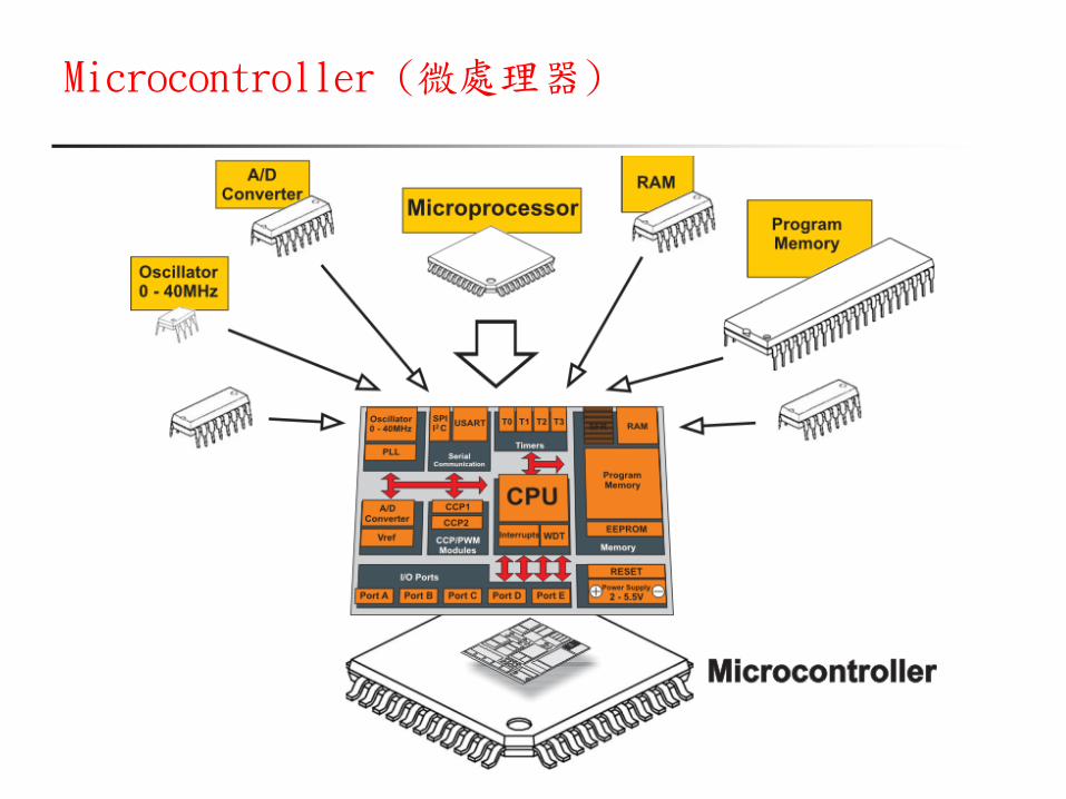
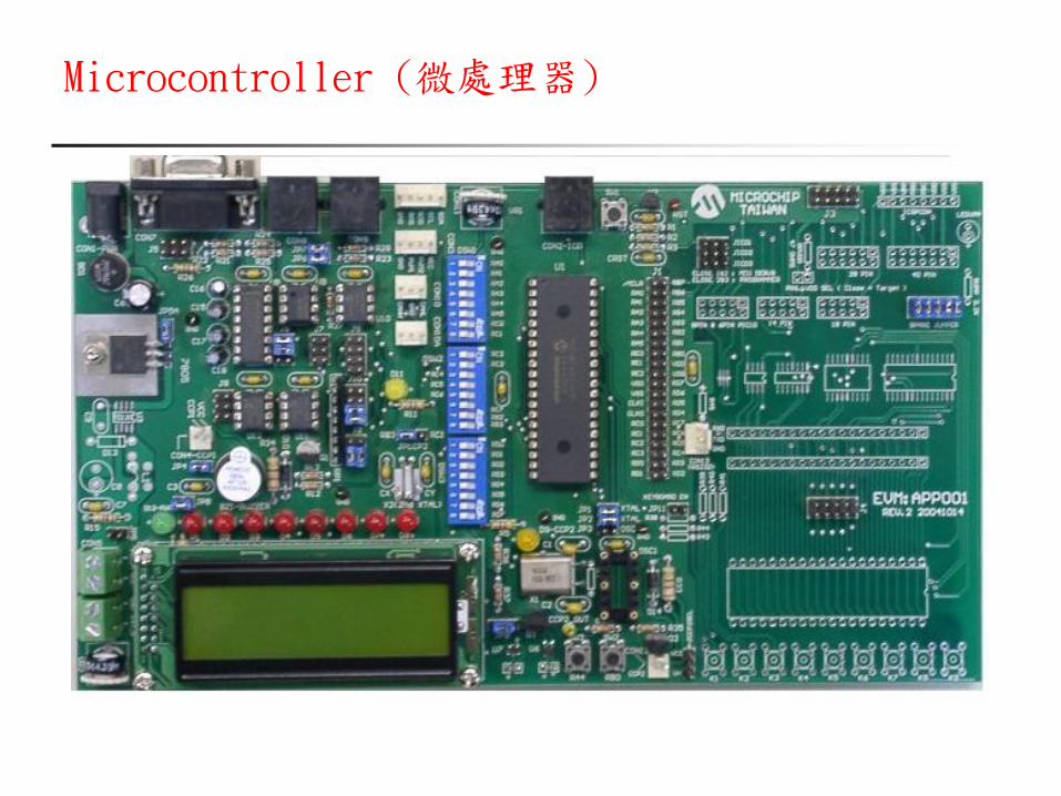
Microcontroller (微處理器)
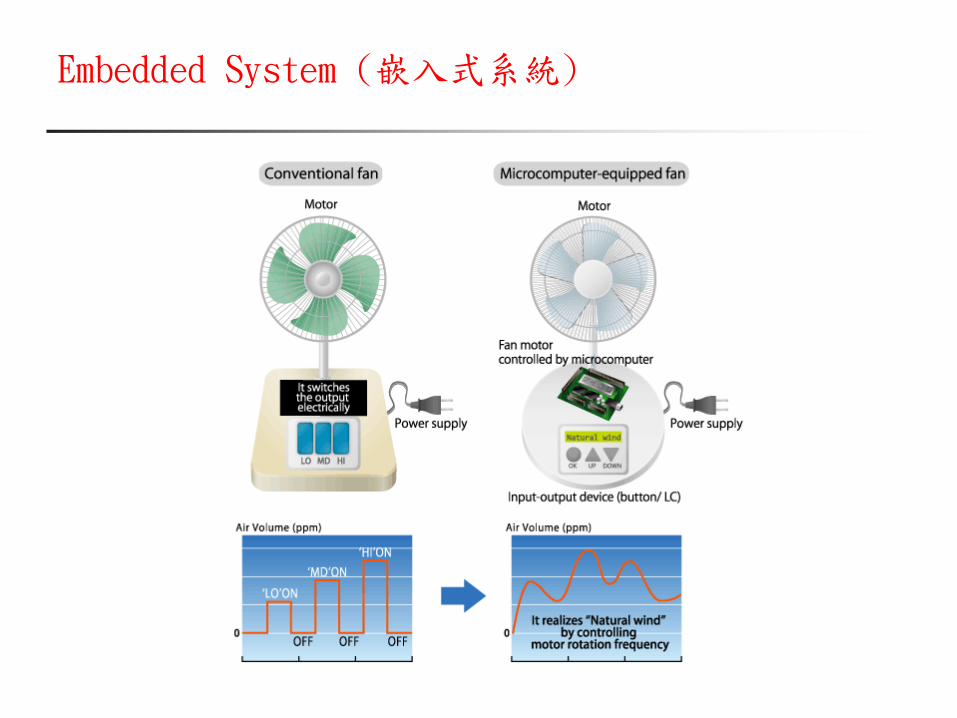
Embedded System (嵌入式系統)
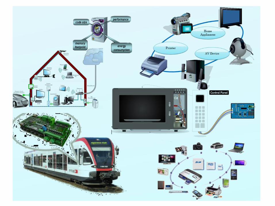
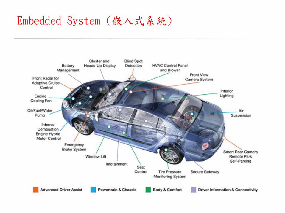
Embedded System (嵌入式系統)
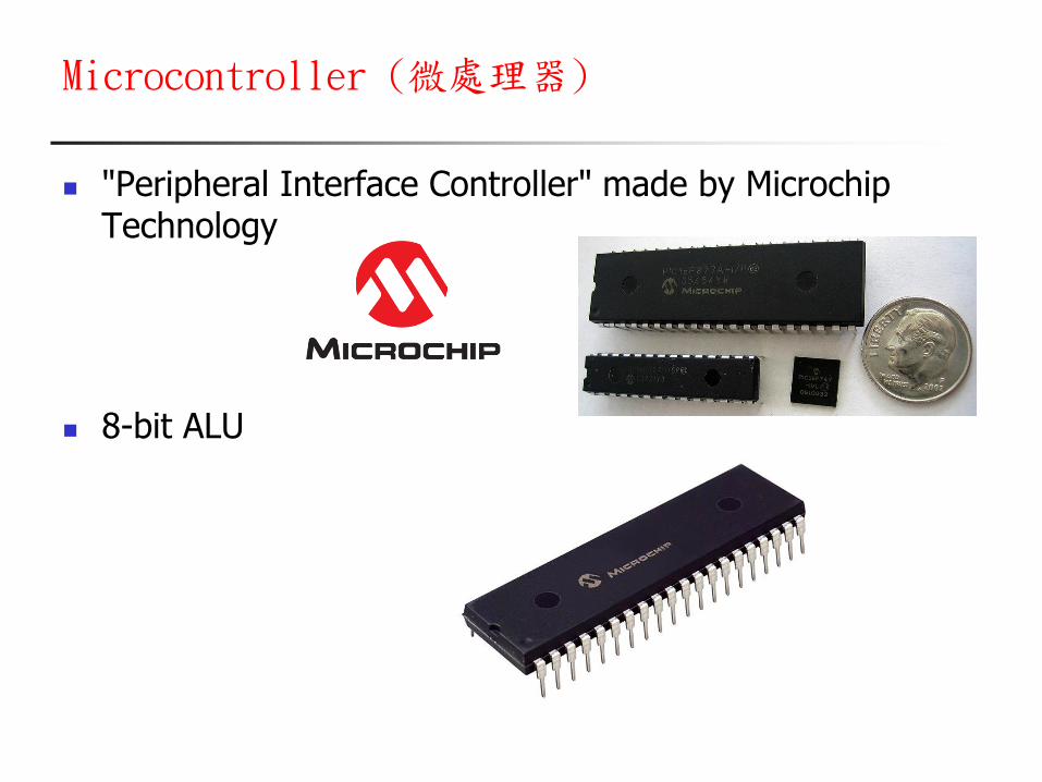
Microcontroller (微處理器)
"Peripheral Interface Controller" made by Microchip Technology
8-bit ALU
Microcontroller (微處理器)
1-1 TURING MODEL
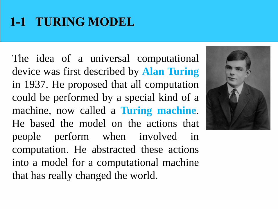
The idea of a universal computational
device was first described by Alan Turing
in 1937. He proposed that all computation
could be performed by a special kind of a
machine, now called a Turing machine.
He based the model on the actions that
people perform when involved in
computation. He abstracted these actions
into a model for a computational machine
that has really changed the world.
Data processors
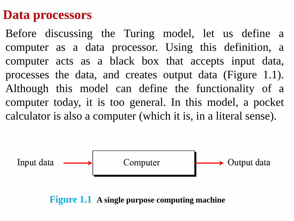
Before discussing the Turing model, let us define a
computer as a data processor. Using this definition, a
computer acts as a black box that accepts input data,
processes the data, and creates output data (Figure 1.1).
Although this model can define the functionality of a
computer today, it is too general. In this model, a pocket
calculator is also a computer (which it is, in a literal sense).
Figure 1.1 A single purpose computing machine
Programmable data processors
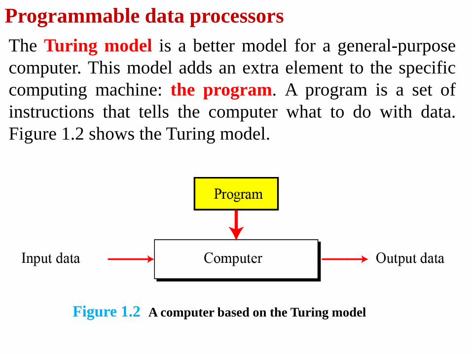
The Turing model is a better model for a general-purpose
computer. This model adds an extra element to the specific
computing machine: the program. A program is a set of
instructions that tells the computer what to do with data.
Figure 1.2 shows the Turing model.
Figure 1.2 A computer based on the Turing model
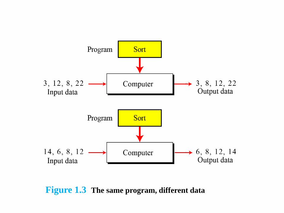
Figure 1.3 The same program, different data
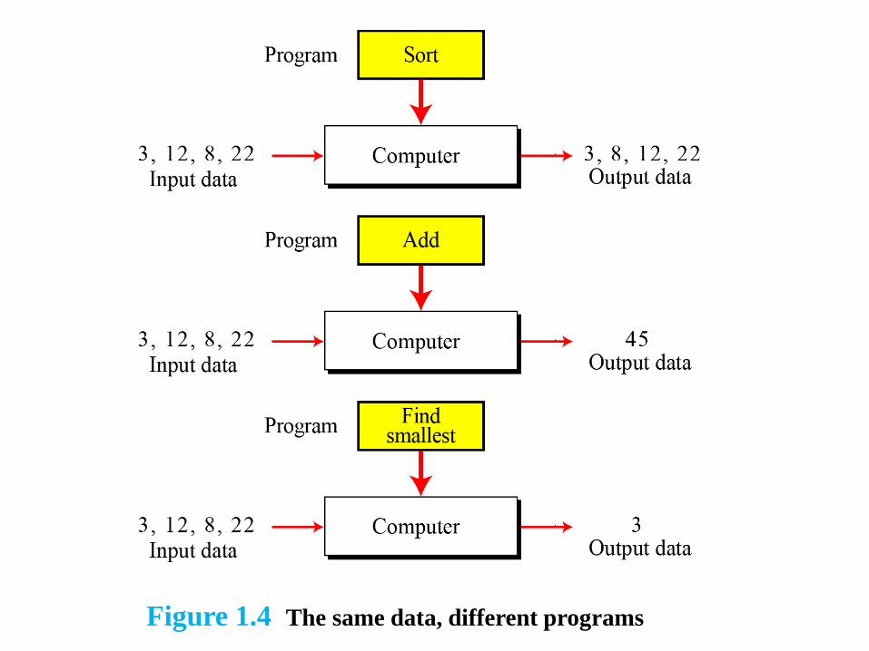
Figure 1.4 The same data, different programs
The universal Turing machine
A universal Turing machine, a machine that can do any
computation if the appropriate program is provided, was the
first description of a modern computer. It can be proved that
a very powerful computer and a universal Turing machine
can compute the same thing. We need only provide the data
and the program—the description of how to do the
computation—to either machine. In fact, a universal Turing
machine is capable of computing anything that is
computable.
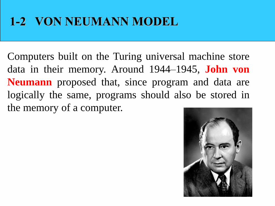
1-2 VON NEUMANN MODEL
Computers built on the Turing universal machine store
data in their memory. Around 1944–1945, John von
Neumann proposed that, since program and data are
logically the same, programs should also be stored in
the memory of a computer.
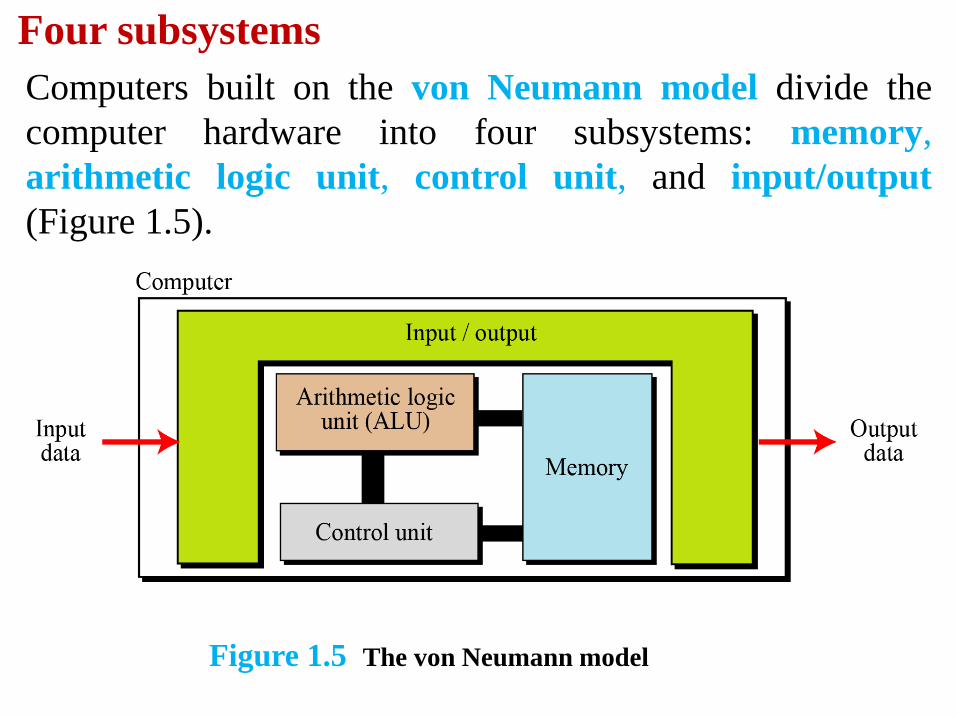
Computers built on the von Neumann model divide the
computer hardware into four subsystems: memory,
arithmetic logic unit, control unit, and input/output
(Figure 1.5).
Four subsystems
Figure 1.5 The von Neumann model
The von Neumann model states that the program must be
stored in memory. This is totally different from the
architecture of early computers in which only the data was
stored in memory: the programs for their task was
implemented by manipulating a set of switches or by
changing the wiring system.
The memory of modern computers hosts both a
program and its corresponding data. This implies that both
the data and programs should have the same format, because
they are stored in memory. In fact, they are stored as binary
patterns in memory — a sequence of 0s and 1s.
The stored program concept
A program in the von Neumann model is made of a finite
number of instructions. In this model, the control unit
fetches one instruction from memory, decodes it, then
executes it. In other words, the instructions are executed one
after another. Of course, one instruction may request the
control unit to jump to some previous or following
instruction, but this does not mean that the instructions are
not executed sequentially. Sequential execution of a program
was the initial requirement of a computer based on the von
Neumann model. Today’s computers execute programs in
the order that is the most efficient.
Sequential execution of instructions
1-3 COMPUTER COMPONENTS
We can think of a computer as being made up of three
components: computer hardware, data, and computer
software.
Computer hardware today has four components under the
von Neumann model, although we can have different types
of memory, different types of input/output subsystems, and
so on. We discuss computer hardware in more detail in
Chapter 2.
Computer hardware
The von Neumann model clearly defines a computer as a
data processing machine that accepts the input data,
processes it, and outputs the result.
Data
The main feature of the Turing or von Neumann models is
the concept of the program. Although early computers did
not store the program in the computer’s memory, they did
use the concept of programs. Programming those early
computers meant changing the wiring systems or turning a
set of switches on or off. Programming was therefore a task
done by an operator or engineer before the actual data
processing began.
Computer software
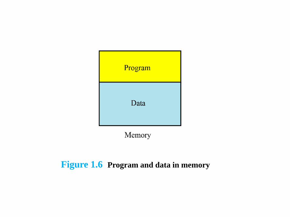
Figure 1.6 Program and data in memory
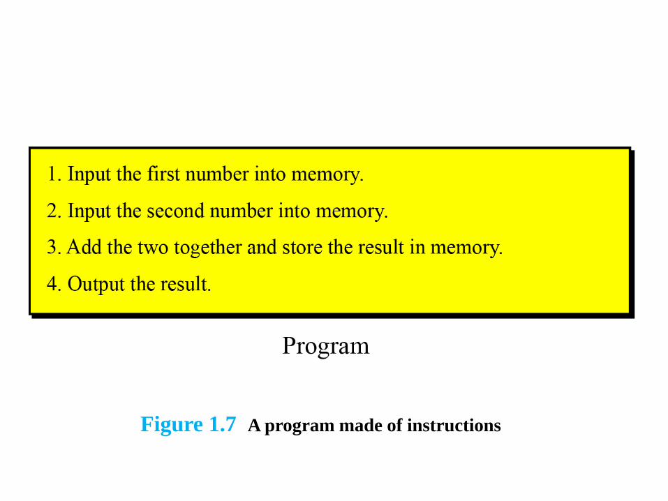
Figure 1.7 A program made of instructions
0-28
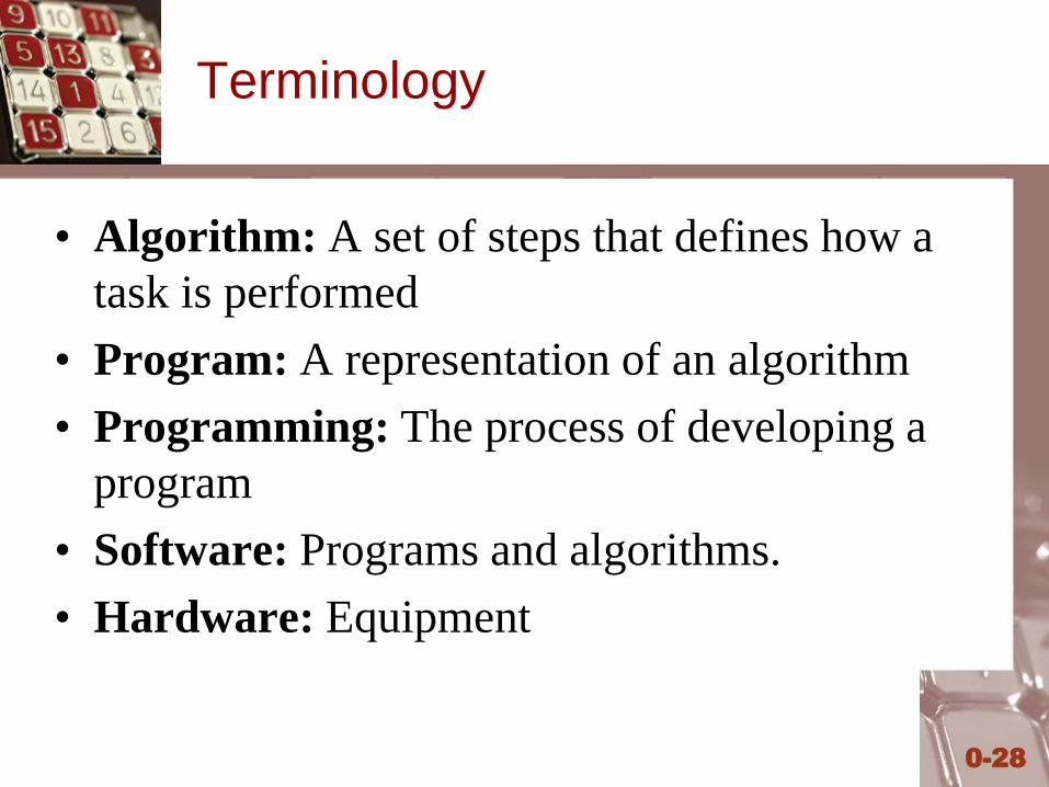
Terminology
• Algorithm: A set of steps that defines how a
task is performed
• Program: A representation of an algorithm
• Programming: The process of developing a
program
• Software: Programs and algorithms.
• Hardware: Equipment
0-29
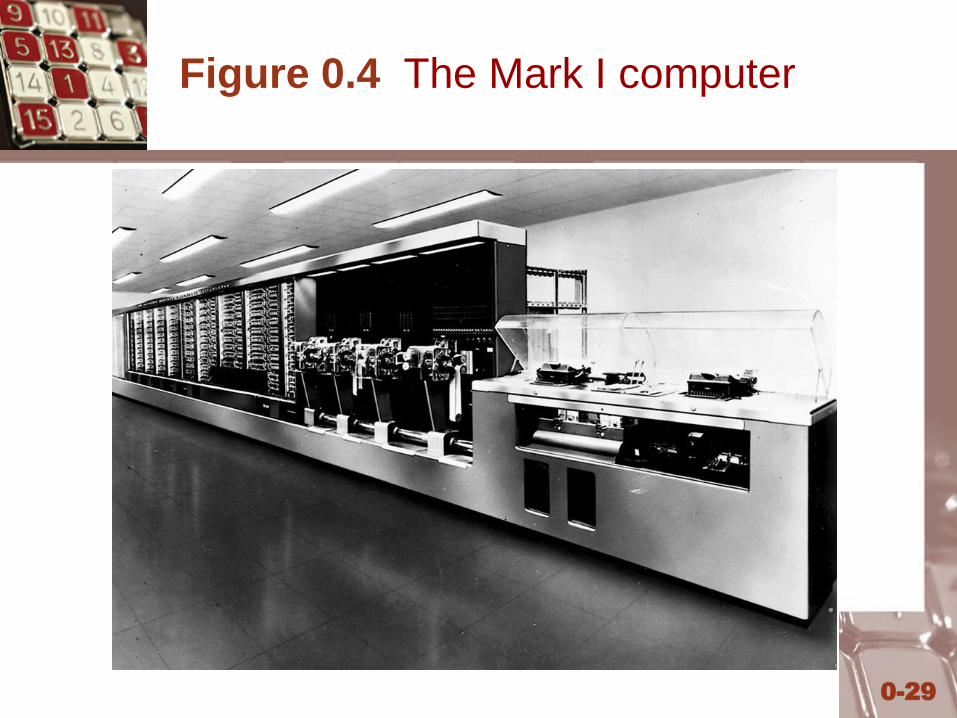
Figure 0.4 The Mark I computer
1-4 HISTORY
In this section we briefly review the history of computing
and computers. We divide this history into three periods.
Mechanical machines (before 1930)
During this period, several computing machines were
invented that bear little resemblance to the modern concept
of a computer.
In the 17th century, Blaise Pascal, a French mathematician and
philosopher, invented Pascaline.
In the late 17th century, a German mathematician called Gottfried
Leibnitz invented what is known as Leibnitz’Wheel.
The first machine that used the idea of storage and programming
was the Jacquard loom, invented by Joseph-Marie Jacquard at the
beginning of the 19th century.
In 1823, Charles Babbage invented the Difference Engine. Later,
he invented a machine called the Analytical Engine that parallels
the idea of modern computers.
In 1890, Herman Hollerith, working at the US Census Bureau,
designed and built a programmer machine that could automatically
read, tally, and sort data stored on punched cards.
The birth of electronic computers (1930–1950)
Between 1930 and 1950, several computers were invented
by scientists who could be considered the pioneers of the
electronic computer industry.
The early computers of this period did not store the program
in memory—all were programmed externally. Five
computers were prominent during these years:
ABC
Z1
Mark I.
Colossus
ENIAC
Early electronic computers
The first computer based on von Neumann’s ideas was made
in 1950 at the University of Pennsylvania and was called
EDVAC. At the same time, a similar computer called
EDSAC was built by Maurice Wilkes at Cambridge
University in England.
Computers based on the von Neumann model
Computer generations (1950–present)
Computers built after 1950 more or less follow the von
Neumann model. They have become faster, smaller, and
cheaper, but the principle is almost the same. Historians
divide this period into generations, with each generation
witnessing some major change in hardware or software (but
not in the model).
The first generation (roughly 1950–1959) is characterized
by the emergence of commercial computers.
First generation
Second-generation computers (roughly 1959–1965) used
transistors instead of vacuum tubes. Two high-level
programming languages, FORTRAN and COBOL invented
and made programming easier.
Second generation
The invention of the integrated circuit reduced the cost and
size of computers even further. Minicomputers appeared on
the market. Canned programs, popularly known as software
packages, became available. This generation lasted roughly
from 1965 to 1975.
Third generation
The fourth generation (approximately 1975–1985) saw the
appearance of microcomputers. The first desktop calculator,
the Altair 8800, became available in 1975. This generation
also saw the emergence of computer networks.
Fourth generation
This open-ended generation started in 1985. It has witnessed
the appearance of laptop and palmtop computers,
improvements in secondary storage media (CD-ROM, DVD
and so on), the use of multimedia, and the phenomenon of
virtual reality.
Fifth generation
© 2007 Pearson Addison-Wesley. All rights reserved 0-38
Computer Architecture
• Central Processing Unit (CPU) or processor
– Arithmetic/Logic unit versus Control unit
– Registers
• General purpose
• Special purpose
• Bus
• Motherboard
© 2007 Pearson Addison-Wesley. All rights reserved 0-39
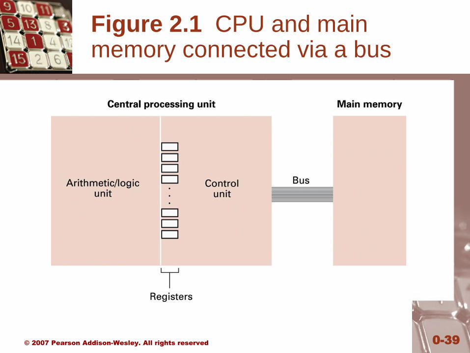
Figure 2.1 CPU and main memory connected via a bus
© 2007 Pearson Addison-Wesley. All rights reserved 0-40
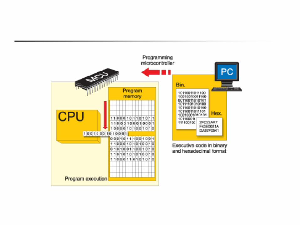
Stored Program Concept
A program can be encoded as bit patterns and
stored in main memory. From there, the CPU
can then extract the instructions and execute
them. In turn, the program to be executed can
be altered easily.
0-41
Questions & Exercises 2.1
1. What information must be the CPU supply to the main memory
circuitry to write a value into a memory cell ?
Ans: The value to be written, the address of the data in which
to write, and the command to write.
© 2007 Pearson Addison-Wesley. All rights reserved 0-42
Terminology
• Machine instruction: An instruction (or
command) encoded as a bit pattern
recognizable by the CPU
• Machine language: The set of all instructions
recognized by a machine
© 2007 Pearson Addison-Wesley. All rights reserved 0-43
Machine Language Philosophies
• Reduced Instruction Set Computing (RISC)
– Few, simple, efficient, and fast instructions
– Example: PowerPC from Apple/IBM/Motorola
• Complex Instruction Set Computing (CISC)
– Many, convenient, and powerful instructions
– Example: Pentium from Intel
CISC
CISC (pronounced sisk) stands for complex instruction set
computer (CISC). The strategy behind CISC architectures is
to have a large set of instructions, including complex ones.
Programming CISC-based computers is easier than in other
designs because there is a single instruction for both simple
and complex tasks. Programmers, therefore, do not have to
write a set of instructions to do a complex task.
RISC
RISC (pronounced risk) stands for reduced instruction set
computer. The strategy behind RISC architecture is to have a
small set of instructions that do a minimum number of
simple operations. Complex instructions are simulated using
a subset of simple instructions. Programming in RISC is
more difficult and time-consuming than in the other design,
because most of the complex instructions are simulated using
simple instructions.
© 2007 Pearson Addison-Wesley. All rights reserved 0-46
Machine Instruction Types
• Data Transfer: copy data from one location to
another
• Arithmetic/Logic: use existing bit patterns to
compute a new bit patterns
• Control: direct the execution of the program
© 2007 Pearson Addison-Wesley. All rights reserved 0-47
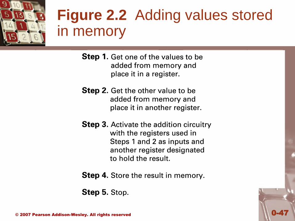
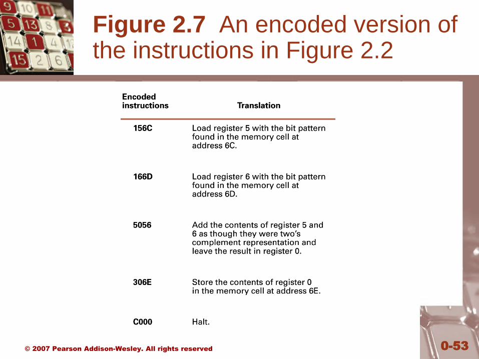
Figure 2.2 Adding values stored in memory
© 2007 Pearson Addison-Wesley. All rights reserved 0-48
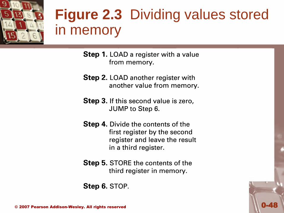
Figure 2.3 Dividing values stored in memory
© 2007 Pearson Addison-Wesley. All rights reserved 0-49
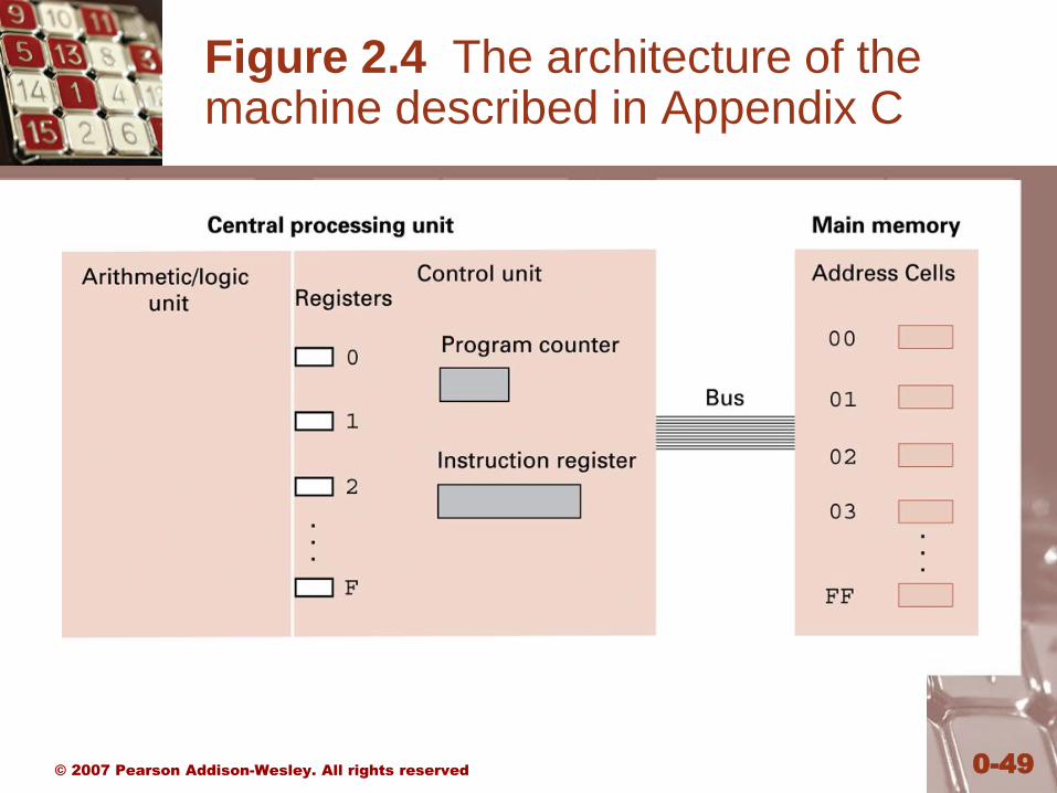
Figure 2.4 The architecture of the machine described in Appendix C
© 2007 Pearson Addison-Wesley. All rights reserved 0-50
Parts of a Machine Instruction
• Op-code: Specifies which operation to execute
• Operand: Gives more detailed information
about the operation
– Interpretation of operand varies depending on op-
code
© 2007 Pearson Addison-Wesley. All rights reserved 0-51
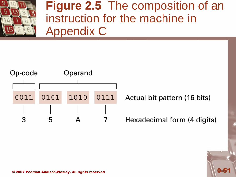
Figure 2.5 The composition of an instruction for the machine in Appendix C
© 2007 Pearson Addison-Wesley. All rights reserved 0-52
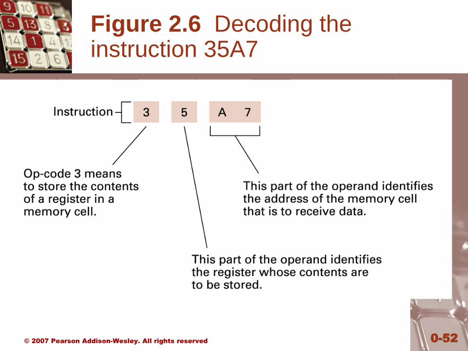
Figure 2.6 Decoding the instruction 35A7
© 2007 Pearson Addison-Wesley. All rights reserved 0-53
Figure 2.7 An encoded version of the instructions in Figure 2.2
© 2007 Pearson Addison-Wesley. All rights reserved 0-54
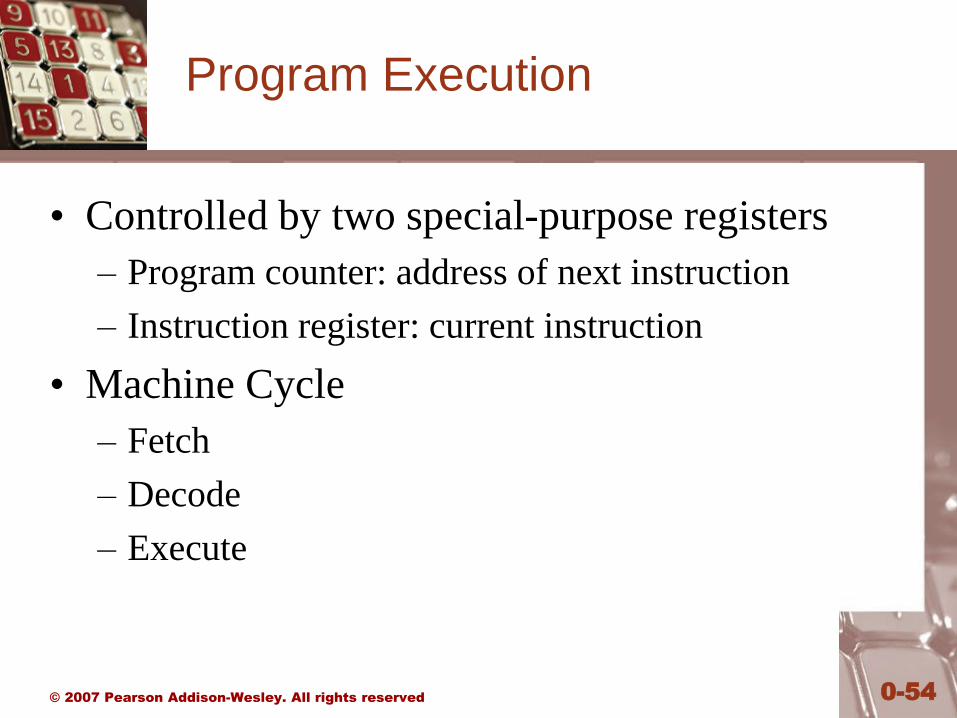
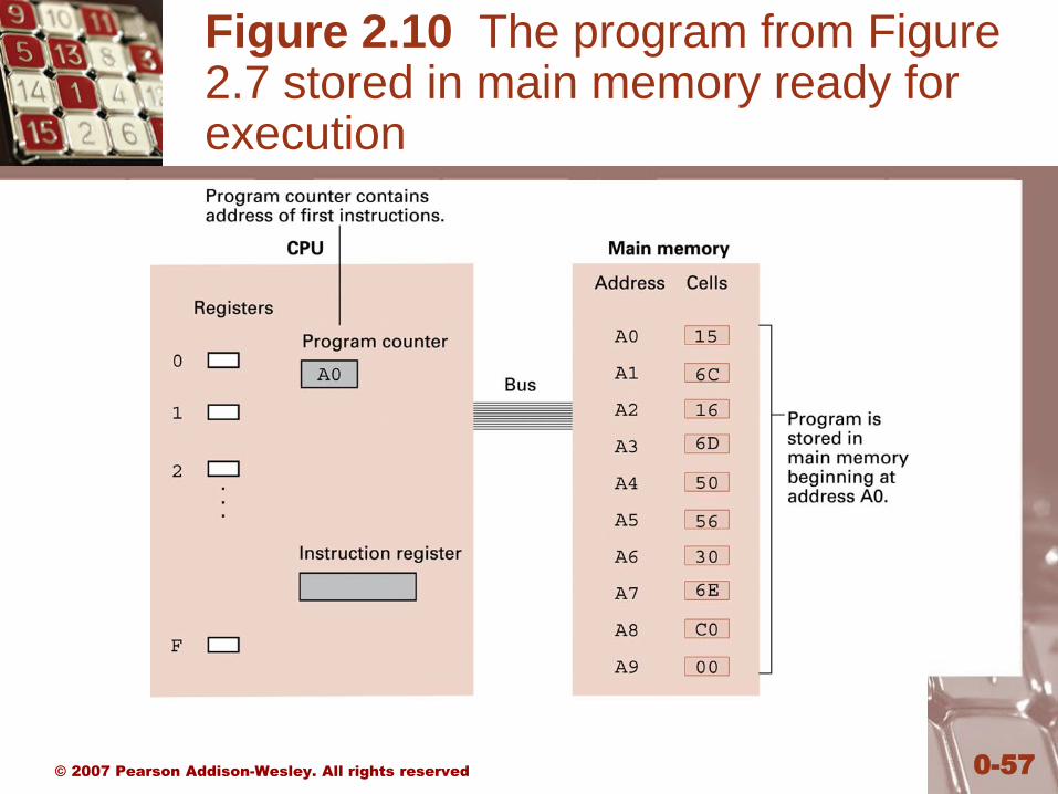
Program Execution
• Controlled by two special-purpose registers
– Program counter: address of next instruction
– Instruction register: current instruction
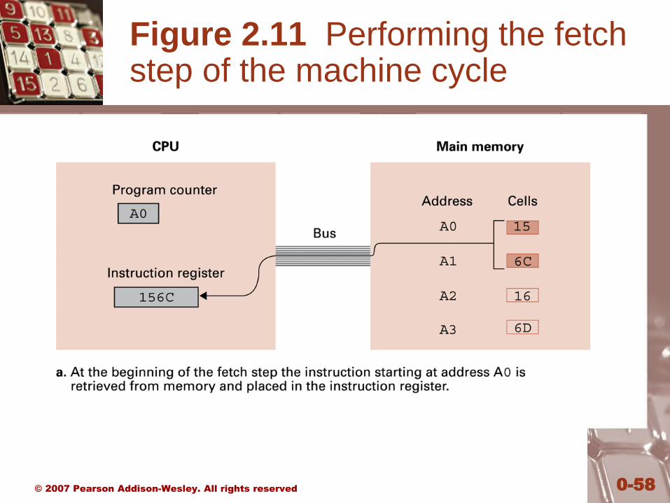
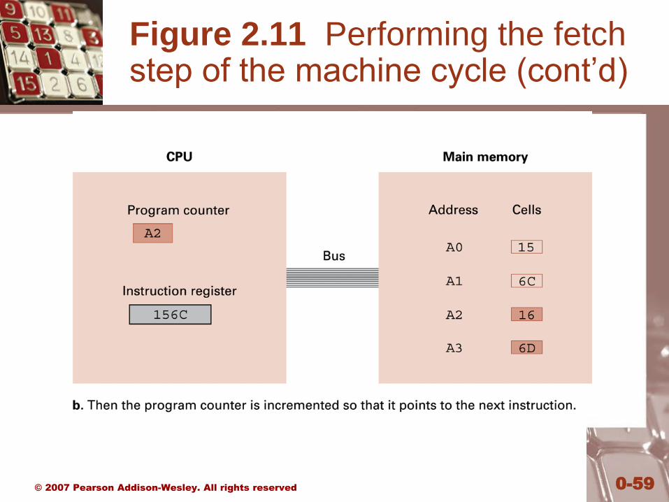
• Machine Cycle
– Fetch
– Decode
– Execute
© 2007 Pearson Addison-Wesley. All rights reserved 0-55
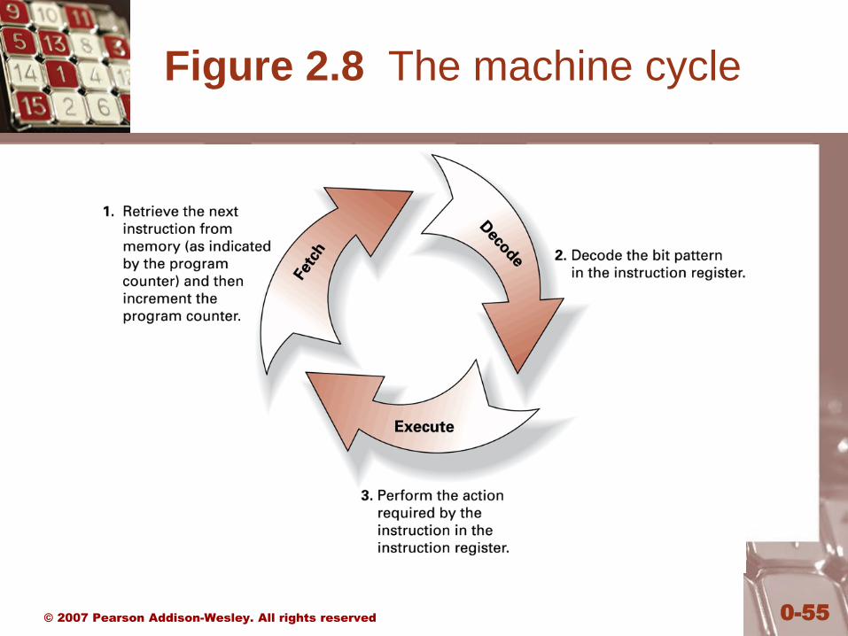
Figure 2.8 The machine cycle
© 2007 Pearson Addison-Wesley. All rights reserved 0-56
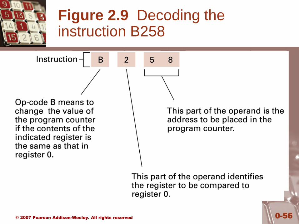
Figure 2.9 Decoding the instruction B258
© 2007 Pearson Addison-Wesley. All rights reserved 0-57
Figure 2.10 The program from Figure 2.7 stored in main memory ready for execution
© 2007 Pearson Addison-Wesley. All rights reserved 0-58
Figure 2.11 Performing the fetch step of the machine cycle
© 2007 Pearson Addison-Wesley. All rights reserved 0-59
Figure 2.11 Performing the fetch step of the machine cycle (cont’d)
© 2007 Pearson Addison-Wesley. All rights reserved 0-60
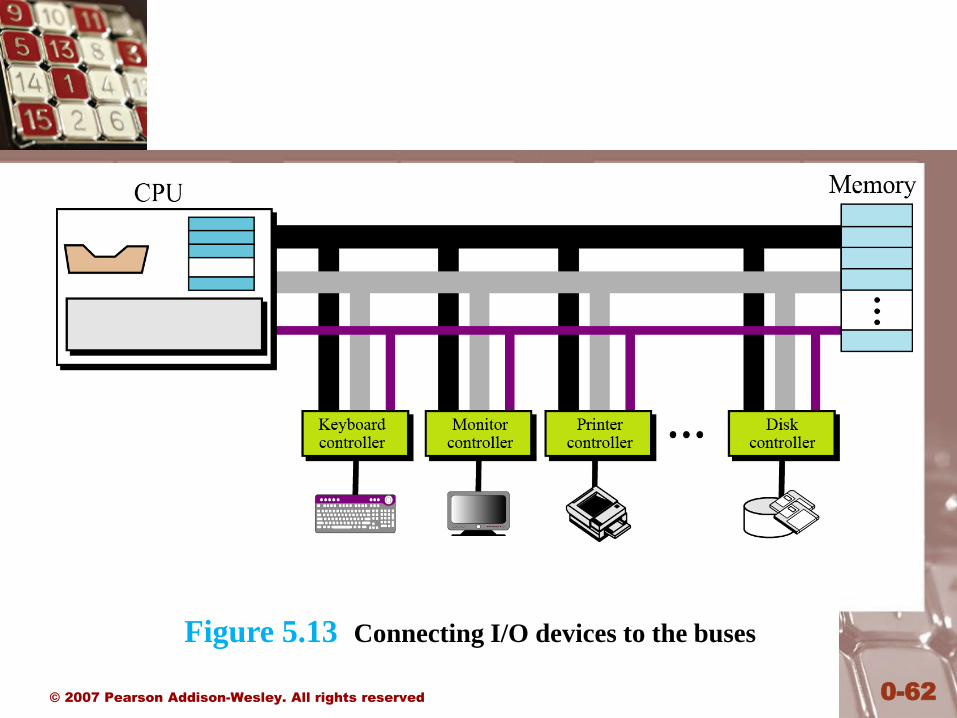
Communicating with Other Devices
• Controller: An intermediary apparatus that handles
communication between the computer and a device
– Specialized controllers for each type of device
– General purpose controllers (USB and FireWire)
• Port: The point at which a device connects to a
computer
• Memory-mapped I/O: CPU communicates with
peripheral devices as though they were memory cells
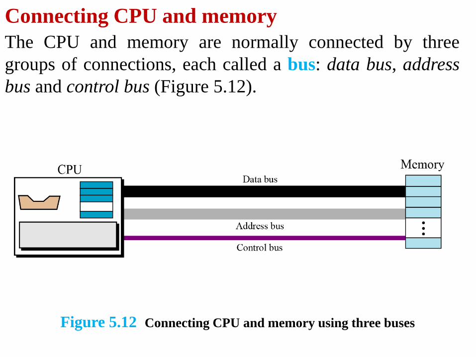
Connecting CPU and memory
The CPU and memory are normally connected by three
groups of connections, each called a bus: data bus, address
bus and control bus (Figure 5.12).
Figure 5.12 Connecting CPU and memory using three buses
© 2007 Pearson Addison-Wesley. All rights reserved 0-62
Figure 5.13 Connecting I/O devices to the buses
© 2007 Pearson Addison-Wesley. All rights reserved 0-63
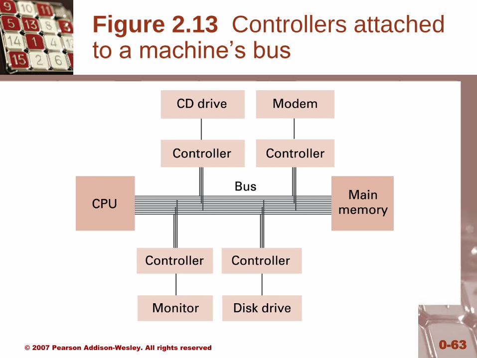
Figure 2.13 Controllers attached to a machine’s bus
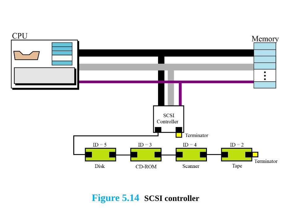
Figure 5.14 SCSI controller
© 2007 Pearson Addison-Wesley. All rights reserved 0-65
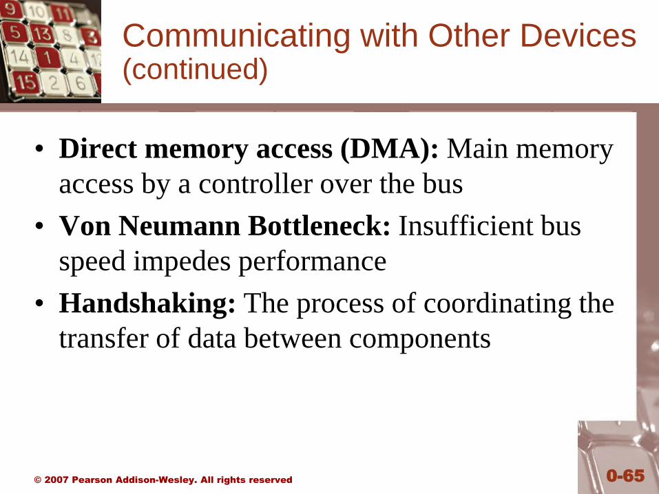
Communicating with Other Devices (continued)
• Direct memory access (DMA): Main memory
access by a controller over the bus
• Von Neumann Bottleneck: Insufficient bus
speed impedes performance
• Handshaking: The process of coordinating the
transfer of data between components
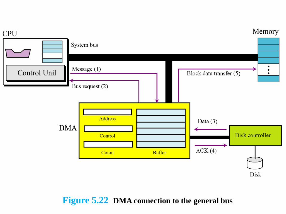
Figure 5.22 DMA connection to the general bus
© 2007 Pearson Addison-Wesley. All rights reserved 0-67
Communicating with Other Devices (continued)
• Parallel Communication: Several communication paths transfer bits simultaneously.
• Serial Communication: Bits are transferred one after the other over a single communication path.
– Serial communication requires a simpler data path than parallel communication. For example, USB and FireWire.
Recommended


