Angelika Wiegele
Nonlinear OptimizationTechniques Applied to
Combinatorial OptimizationProblems
DISSERTATION
zur Erlangung des akademischen GradesDoktorin der Technischen Wissenschaften
Alpen-Adria- Universi tät Klagenfurt
Fakultät für Wirtschaftswissenschaften und Informatik
1. Begutachter: Univ.-Prof. Dipl.-Ing. Dr. Franz RendlInstitut für Mathematik
2. Begutachterin: Ao. Univ.-Prof. Dipl.-Ing. Dr. Christine NowakInstitut für Mathematik
Oktober 2006

Ehrenwörtliche ErklärungIch erkläre ehrenwörtlich, dass ich die vorliegende Schrift verfasst und die mit ihrunmittelbar verbundenen Arbeiten selbst durchgeführt habe. Die in der Schriftverwendete Literatur sowie das Ausmaß der mir im gesamten Arbeitsvorgang ge-währten Unterstützung sind ausnahmslos angegeben. Die Schrift ist noch keineranderen Prüfungsbehörde vorgelegt worden.
Klagenfurt, Oktober 2006
Abstract
Combinatorial Optimization and Semidefinite Programming are two research top-ics that have attracted the attention of many mathematicians and computer sci-entists during the past two decades. Remarkable results have been achieved inboth fields. This thesis is a further component in exploring the field of Semidefi-nite Programming and investigating Combinatorial Optimization problems.
Due to the various areas of application, one research topic of high interestis the development of algorithms for solving Semidefinite Programs. Althoughreliable methods are already available and widely used these algorithms are ofteninapplicable for large-scale programs, due to the huge memory requirements orthe vast computational effort. The present work proposes methods (and imple-mentations) that are capable of solving Semidefinite Programs of high dimensionsand/or a large number of constraints. These methods are: the Bundle Methodapplied to solve Semidefinite Programs, the Spectral Bundle Method with secondorder information, and the Boundary Point Method.
Exploiting the concept of Bundle Methods allows solving problems, even ifthe number of .constraints is rather large. By the use of Lagrange multipliers, theconstraints (or some of them) are lifted into the objective function and the dualproblem is then solved following the concept of Bundle Methods.
In the Spectral Bundle Method the largest Eigenvalue Àmax of a matrix isminimized. Since the second-order behavior of the Àmax function is well studied,it can be incorporated in this method. Making partial use of this second-orderinformation improves the efficiencyof the Spectral Bundle Method while keepingit computationally practical.
Another new algorithm for solving Semidefinite Programs is the BoundaryPoint Method. This is an augmented Lagrangian algorithm applied to solveSemidefinite Programs. For various problem classes this method is by far superiorto other available algorithms.
Regarding applications, the main focus of this study is on the Max-Cut prob-lem, one of the most challenging Combinatorial Optimization problems. Theapplicability of this problem is even broader than obvious at first sight, since anyunconstrained quadratic (0-1) problem can be transformed to a Max-Cut prob-lem. Apart from recalling the properties of the problem and giving a survey ofrelaxations and known solution methods, new relaxations based on Semidefinite

11
Programming are introduced. Finally, "Biq Mac" was developed, a solver forbinary quadratic and Max-Cut problems. Biq Mac is an implementation of anexact solution method using a Branch & Bound algorithm with a bounding rou-tine based on Semidefinite Programming. Detailed information on this algorithm,as well as a collection of test problems together with numerical results, can befound in the present thesis. Various test problems that have been considered inthe literature for years, were solved by Biq Mac for the first time. This affirmsthe success of using Semidefinite Programming for Combinatorial Optimizationproblems.
Acknowledgements
I am grateful to a number of people who have supported me in the developmentof this work and it is my pleasure now to highlight them here.
I want to thank my supervisor Franz Rendl for introducing me into the fieldof Semidefinite Programming, for his enthusiasm about discussing mathematicalissues and for the large amount of time he devoted to my concerns. His ideas andadvice led me into active research and substantiated my thesis.
The Mathematics Department at the Alpen-Adria-Universität Klagenfurt pro-vided excellent working conditions. I would like to thank my colleagues at thedepartment and especially Christine Nowak. She served as a member of my Ph.D.committee and she was willing to encourage me at any time.
I also want to thank Giovanni Rinaldi for inviting me to IASI-CNR in Rome.Due to him and the people in his group my research stays in Rome were veryfruitful and enjoyable. Furthermore, I gratefully acknowledge financial supportfrom the EU project Algorithmic Discrete Optimization (ADONET), MRTN-CT-2003-504438. Participation at various conferences and workshops, as well asthe research stay at IASI-CNR in Rome were financed by this research trainingnetwork.
Having people around to have fun with, to discuss whatever has to be dis-cussed, to fill my spare time with joyful events, but also to understand thatsometimes 'spare time' is negligibly small, is very important for me. I am grate-ful for being surrounded by such friends and for the many occasions that provedhow precious they are to me.
Above all, my thanks go to my family. Although I was away quite often, Ialways had a hearty welcome when returning home. I want to dedicate this workto them.
III

Contents
Abstract
Acknowledgements
Notation
Introduction
1 Semidefinite Programming1.1 The Semidefinite Programming Problem1.2 Duality Theory . . . . .1.3 Eigenvalue Optimization .1.4 On Solving Semidefinite Programming Problems
1.4.1 Interior-Point Methods .1.4.2 Spectral Bundle Method . . . . . . . . .1.4.3 Software for Solving Semidefinite Programs.
2 Combinatorial Optimization2.1 The Max-Cut Problem . . .2.2 The Stable Set Problem ..2.3 The Graph Partitioning Problem2.4 The Max-Sat Problem . . .
3 The Maximum Cut Problem3.1 Properties of the Max-Cut Problem . . . . . . . . .3.2 Quadratic (0-1) Programming and Relation to MC
3.2.1 (QP)~ (MC) .3.2.2 (MC)~ (QP) .3.2.3 (MC) vs. (QP) .
3.3 Relaxations of the Max-Cut Problem3.3.1 Relaxations Based on Linear Programming.3.3.2 A Basic SDP Relaxation . . .3.3.3 Convex Quadratic Relaxations .3.3.4 Second-Order Cone Programming Relaxations
v
iii
ix
1
3458
101013161718192022
2323252526272727303233
VI CONTENTS
3.3.5 Branch & Bound with Preprocessing 333.4 A Rounding Heuristic Based on SDP . . . . 34
4 SDP Relaxations of the Max-Cut Problem 354.1 The Basic Relaxation. . . . . . . . 354.2 Strengthening the Basic Relaxation . . . . . 364.3 Lift-and-Project Methods 37
4.3.1 The Lifting of Anjos and Wolkowicz . 374.3.2 The Lifting of Lasserre . . . . . . . . 41
4.4 Between the Basic Relaxation and a First Lifting 424.4.1 Exploiting Sparsity . . . . . . . . . . . 434.4.2 Systematically Chosen Submatrices . . 464.4.3 Numerical Results of (MCSPARSE) . 47
5 Algorithms for solving large-scale SDPs 495.1 The Bundle Method in Combinatorial Optimization 50
5.1.1 Solving (MCSPARSE) Using the Bundle Method 515.1.2 Solving (SDPMET) Using the Bundle Method 54
5.2 Spectral Bundle with 2nd Order Information . . . . 585.3 A Boundary Point Method . . . . . . . . . . . . . . 645.4 A Recipe for Choosing the Proper Solution Method 68
6 Biq Mac 716.1 A Branch & Bound Framework for (MC) . 716.2 Branching Rules. . . 73
6.2.1 Easy First . . . . 746.2.2 Difficult First . . 746.2.3 A Variant of R3 . 746.2.4 Strong Branching 74
6.3 Implementation of the Biq Mac Solver 776.4 The Biq Mac Library. . . 80
6.4.1 Max-Cut...... 836.4.2 Instances of (QP) . 84
6.5 Numerical Results. . . . . 856.5.1 Numerical Results of (MC) Instances. 886.5.2 Numerical Results of (QP) Instances 91
6.6 Extensions........... 926.6.1 The Bisection Problem . 926.6.2 Max-2Sat . . . . . . . . 936.6.3 The Stable Set Problem 946.6.4 The Quadratic Knapsack Problem. 95
6.7 Concluding Remarks on Biq Mac . . . . . 95
CONTENTS
Summary and Outlook
A Background MaterialA.1 Positive Semidefinite MatricesA.2 Convexity, Minimax Inequality.
B Problem GenerationB.1 rudy Calls . . . . . . . . . . . . . . . . . . .B.2 Pardalos-Rodgers Generator Parameters ..
B.2.1 Parameters for the bqpgka InstancesB.2.2 Parameters for the bqpbe Instances
C Tables with Detailed Numerical Results
Bibliography
Index of Keywords
vu
97
9999
100
101101102102103
105118129
Notation
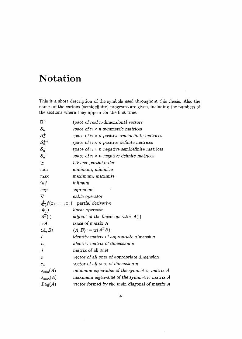
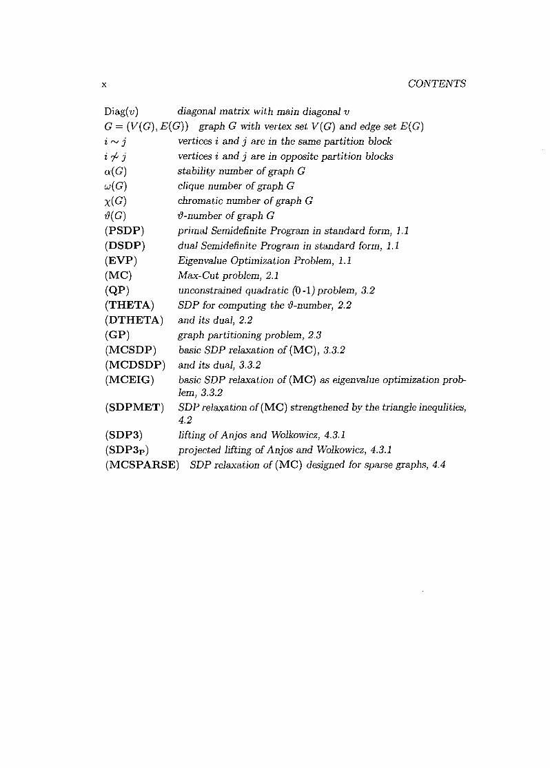
This is a short description of the symbols used throughout this thesis. Also thenames of the various (semidefinite) programs are given, including the numbers ofthe sections where they appear for the first time.
]Rn
SnS+ns++n
S;;S;;->-mm
maxin!
space of real n-dimensional vectorsspace of n x n symmetric matricesspace of n x n positive semidefinite matricesspace of n x n positive definite matricesspace of n x n negative semidefinite matricesspace of n x n negative definite matricesLöwner partial orderminimum, minimizemaximum, maximizeinfimum
sup supremum\7 nabla operatora~J(Xl' ... 1 xn) partial derivativeA( .) linear operatorAT (.) adjoint of the linear operator A( .)trA trace of matrix A(A,B)I
e
Àmin(A)Àmax(A)diag(A)
(A, B) := tr(AT B)identity matrix of appropriate dimensionidentity matrix of dimension nmatrix of all onesvector of all ones of appropriate dimensionvector of all ones of dimension nminimum eigenvalue of the symmetric matrix Amaximum eigenvalue of the symmetric matrix Avector formed by the main diagonal of matrix A
IX
x CONTENTS
Diag( v) diagonal matrix with main diagonal vG = (V(G), E(G)) graph G with vertex set V(G) and edge set E(G)'/, r-v J vertices i and j are in the same partition blocki rf j vertices i and j are in opposite partition blocksa( G) stability number of graph Gw( G) clique number of graph Gx( G) chromatic number of graph G'l9( G) 'l9-number of graph G(PSDP) primal Semidefinite Program in standard form, 1.1(DSDP) dual Semidefinite Program in standard form, 1.1(EVP) Eigenvalue Optimization Problem, 1.1(MC) Max-Cut problem, 2.1(QP) unconstrained quadratic (0 -1) problem, 3.2(THETA) SDP for computing the 'l9-number, 2.2(DTHETA) and its dual, 2.2(GP) graph partitioning problem, 2.3(MCSDP) basic SDP relaxation of (MC), 3.3.2(MCDSDP) and its dual, 3.3.2(MCEIG) basic SDP relaxation of (MC) as eigenvalue optimization prob-
lem,3.3.2(SDPMET) SDP relaxation of(MC) strengthened by the triangle inequlities,
4.2(SDP3) lifting of Anjos and Wolkowicz, 4.3.1(SDP3p) projected lifting of Anjos and Wolkowicz, 4.3.1(MCSPARSE) SDP relaxation of (MC) designed for sparse graphs, 4.4
Introduction
This thesis is basically concerned with two topics:
• The Max-Cut problem: introducing new relaxations based on SemidefiniteProgramming to obtain tight upper bounds and developing an exact solu-tion method.
• Methods for solving large-scale Semidefinite Programs.
In order to make this thesis self-contained, we explain in Chapter 1 the basicsabout Semidefinite Programming and sketch the two most popular methods forsolving Semidefinite Programs, namely Interior-Point methods and the SpectralBundle Method. In Chapter 2 an introduction to Combinatorial Optimizationand some of the problems arising in this field are given.
One of these problems arising from Combinatorial Optimization is the Max-Cut problem. We concentrate in this thesis on this NP-complete problem andtherefore, Chapter 3 gives a more detailed description and explains methods forfinding upper bounds or solving it. Furthermore it is shown in this chapter thatsolving Max-Cut problems and solving unconstrained quadratic (0-1) problemsis essentially the same. Therefore and since many real-world problems can beformulated as unconstrained quadratic (0-1) problems, it is even more strikingto have an algorithm that solves Max-Cut problems efficiently.
Chapter 4 is concerned with the Max-Cut problem as well. Within this chap-ter we take a closer look on relaxations based on Semidefinite Programming.Apart from those relaxations that work with matrix variables indexed by thevertex-set of the underlying graph, we also consider methods that apply a lift-and-project strategy. The latter relaxations, although being of highly theoret-ical interest, are practically not computable, already for medium-sized graphs.We introduce a new relaxation, that can be viewed as 'lying between' the basicsemidefinite-programming relaxation and a first lifting, and that is solvable alsofor graphs on a few hundred nodes.
Having various Semidefinite Programming formulations that can provide boundsfor NP-hard problems leads naturally to the demand of algorithms for solvingthese Semidefinite Programs. This issue is addressed in Chapter 5. We sketchthere the concept of Bundle Methods and apply this concept to solving Semidef-inite Programs, in particular we design the algorithm for solving two of the re-
1
2 CONTENTS
laxations introduced in Chapter 4. Furthermore, we come back to the SpectralBundle Method, which we equip with a second order model. And as a furtheralgorithm, the Boundary Point Method is introduced within this chapter. Thisnew method elaborates the idea of using the augmented Lagrangian algorithmfor solving Semidefinite Programs.
The final chapter of this thesis, Chapter 6, provides an exact solution methodfor Max-Cut problems. The Biq Mac solver for solving Binary Quadratic andMax- Cut problems is explained. Apart from the ingredients of this solver, Le.a Branch & Bound framework, branching rules, implementation issues, etc., alsoa wide variety of test problems are collected and detailed numerical results aregiven.
Summarizing, this thesis provides the following new studies:
• A relaxation for sparse Max-Cut problems based on Semidefinite Program-ming (Section 4.4) and implementation of the Bundle Method to solve thisrelaxation (Section 5.1.1). This ongoing research can partly be found in[113] .
• Exploiting second order information in the spectral bundle method (Sec-tion 5.2). See also the working paper [4].
• A boundary point method for solving Semidefinite Programs (Section 5.3).This work has been published in [110].
• Developing and implementing Biq Mac, an exact solution algorithm forsolving Max-Cut and unconstrained (0-1) problems. Furthermore, a collec-tion of test problems has been built up and numerical results are presented(Chapter 6). A technical report [115]is available.
Chapter 1
Semidefinite Programming
Many real-world applications, although being non-linear, can be well described bylinearized models. Therefore, Linear Programming (LP) became a widely studiedand applied technique in many areas of science, industry and economy.
Semidefinite Programming (SDP) is an extension of LP. A matrix-variableis optimized over the intersection of the cone of positive-semidefinite matriceswith an affine space. It turned out, that SDP can provide significantly strongerpractical results than LP. The study of SDP goes back to the sixties, when Bell-man and Fan [19]derived theoretical properties of Semidefinite Programs. A firstapplication appeared in the work of Lovasz [88]. Since then SDP turned out tobe practical in a lot of different areas, like combinatorial optimization, controltheory, and more recently in polynomial optimization.
Due to the numerous areas of applications, also solving SDPs became a widelystudied subject. Interior-Point Methods are the most popular algorithms nowa-days. Recently the concept of Bundle Methods also has been applied for solvingSemidefinite Programs.
In this chapter we formulate the Semidefinite Programming problem includingduality theory. A subsection is dedicated to a related problem, namely Eigen-value Optimization. Finally, Interior-Point Algorithms and the Spectral BundleMethod, two algorithms for solving Semidefinite Programs are explained.
Most of the proofs of Theorems and Lemmas in this section are omitted,because they appear in a wide variety of text-books or survey papers. For surveyson SDP the reader is referred to e.g. Helmberg [52],Vandenberghe and Boyd [126],Laurent and Rendl [80]. More references are given in the subsequent sections.
3
4 CHAPTER 1. SEMIDEFINITE PROGRAMMING
1.1 The Semidefinite Programming Problem
A Semidefinite Program in its standard notation is given as follows. Let C andAl, ... , Am be matrices in Sn and b E ]Rm, we obtain
(PSDP) max (C,X)s.t. A(X) = b
X E Sn, X t: 0
where A: Sn -+ ]Rm denotes a linear operator defined as
The adjoint operator AT: ]Rm -+ Sn, is defined through the equation
(A(X), y) = (X, AT(y)), for all X E Sn, Y E ]Rm. (1.1)
Therefore,m m m
(A(X), y) = LYi(Aï, X) = L(YiAi,X) = (LYiAï, X) = (AT(y), X)
and hence,
i=l i=l
m
AT(y) = LYiAï.i=l
i=l
In order to derive the dual to (PSDP), we introduce y E ]Rm to be the Lagrangianmultiplier for the equations in (PSDP). Then the following always hold:
max{ (C, X): A(X) = b, XES:} max min (C, X) - (A(X) - b, y)XES;; yElRm
< min max (b, y) - (AT(y) - C, X)yElRm XES;
min{ (b, y): AT(y) - CES:, Y E ]Rm}.
The first equation is true, because if A(X) = b is not fulfilled, the minimizationyields -00 and conversely, if the equation is satisfied, (C, X) is the result, i.e.
min (C X) _ (A(X) _ b ) = {(C,X) for A(~) = byElRm ' , Y -00 otherwlse. (1.2)
The inequality arises because of Lemma A.11 and for the last equation similarideas as for the first hold, namely
max (b ) _ (AT( ) _ C X) = { (b, y) for AT~y) - C E s;t (1.3)XES; , Y y, 00 otherwlse.

1.2. DUALITY THEORY
Therefore, the dual to (PSDP) can be stated as
(DSDP) mm (b, y)s.t. AT(y) - C = Z
Y E IRm, Z E Sn, Z ~ o.
5
For referring to points satisfying the constraints in (PSDP) or (DSDP),respectively, the following definitions will be useful:
Definition 1.1 (feasibility)Matrix XES; is feasible Jar (PSDP) iJ A(X) = b holds.The pair (y, Z) E IRmx S; is feasible Jar (DSDP) iJ AT(y) - C = Z.
Definition 1.2 (strict feasibility)Matrix X E S;+ is strictly feasible Jar (PSDP) iJ A(X) = b holds.The pair (y, Z) E IRmx S;+ is strictly feasible Jar (DSDP) iJ AT(y) - C = Z.
1.2 Duality Theory
In Section 1.1 we introduced the primal and dual formulation of an SDP in stan-dard form by using Lagrangian multipliers. Let X be a primal feasible solutionand (y, Z) a dual feasible solution, then the difference between the objectivevalues of the primal and dual feasible solution is defined as duality gap.
Definition 1.3 (duality gap) Let XES; and (y, Z) E (IRm x S;), X beingJeasible Jar (PSDP) and (y, Z) being Jeasible Jar (DSDP). The duality gap at(X, y, Z) is given by
(b, y) - (C, X).
Due to Lemma AA, the duality gap is always non-negative:
(b,y) - (C,X) = (A(X),y) - (AT(y) - Z,X) = (Z,X) ~ O. (lA)
This fact is called weak duality and we formulate it as the following
Lemma 1.4 (weak duality) LetX ES;, y E IRmwithA(X) = b andAT(y)-CES;. Then
(C,X)::; (b,y).
If X, yare feasible and the duality gap is zero, then strong duality holds and wehave a proof, that these are the optimal solutions for (PSDP) and (DSDP),respectively. On the other hand, strong duality does not necessarily hold forSDPs, as Vandenberghe and Boyd [126] exemplify:
6 CHAPTER 1. SEMIDEFINITE PROGRAMMING
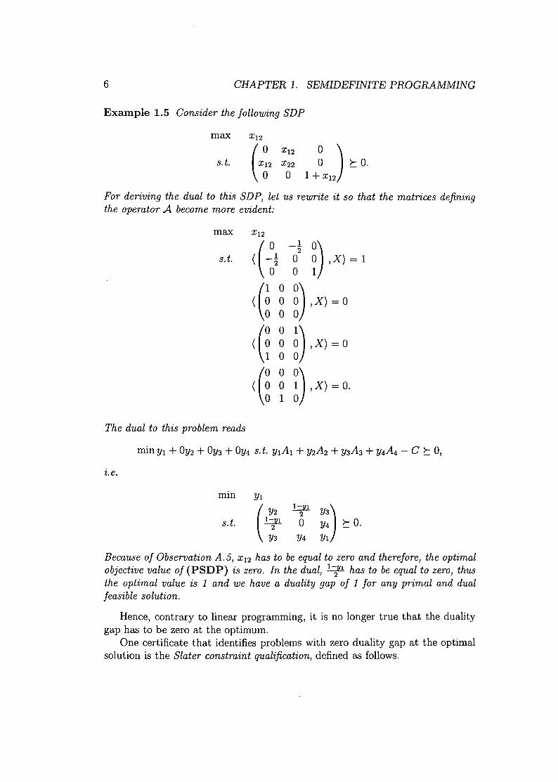
Example 1.5 Consider the following SDP
max
s.t. ~ ) tO.1+ XI2
For deriving the dual to this SDP, let us rewrite it so that the matrices definingthe operator A become more evident:
max
s.t.
The dual to this problem reads
XI2
(( ~l
(
1 0( 0 0
o 0
(
0 0( 0 0
1 0
(
0 0( 0 0
o 1
_1 0)0
20 ,X)=1
o 1
n,X) = 0
n,X) = 0
n,X) =0.
z.e.
mm
s.t. l=lll)2 Y3o Y4 tO.
Y4 YI
Because of Observation A.5, X12 has to be equal to zero and therefore, the optimalobjective value of (PSDP) is zero. In the dual, I-t has to be equal to zero, thusthe optimal value is 1 and we have a duality gap of 1 for any primal and dualfeasible solution.
Hence, contrary to linear programming, it is no longer true that the dualitygap has to be zero at the optimum.
One certificate that identifies problems with zero duality gap at the optimalsolution is the Slater constraint qualification, defined as follows.
1.2. DUALITY THEORY 7
Definition 1.6 (Slater constraint qualification)(PSDP) satisfies the Slater condition if there exists X E S:+ with A(X) = b.(DSDP) satisfies the Slater condition if there exists a pair (y, Z) with Z E S:+and AT(y) - Z = C.
We can provide the following
Theorem 1.7 Denote
p* = sup{ (C, X): A(X) = b,X E s;t}
andd* = inf{ (b, y): AT(y) - CE s;t} .
• If (PSDP) satisfies the Slater condition with p* finite, then p* = d* andthis value is attained for (DSDP) .
• If (DSDP) satisfies the Slater condition with d* finite, then p* = d* isattained for (PSDP) .
• If (PSDP) and (DSDP) both satisfy the Slater condition, then p* = d* isattained for both problems.
A proof can be found for instance in Duffin [34], Nesterov and Nemirovskii [98]or Rockafellar [117]. Obviously, these conditions do not hold for Example 1.5.
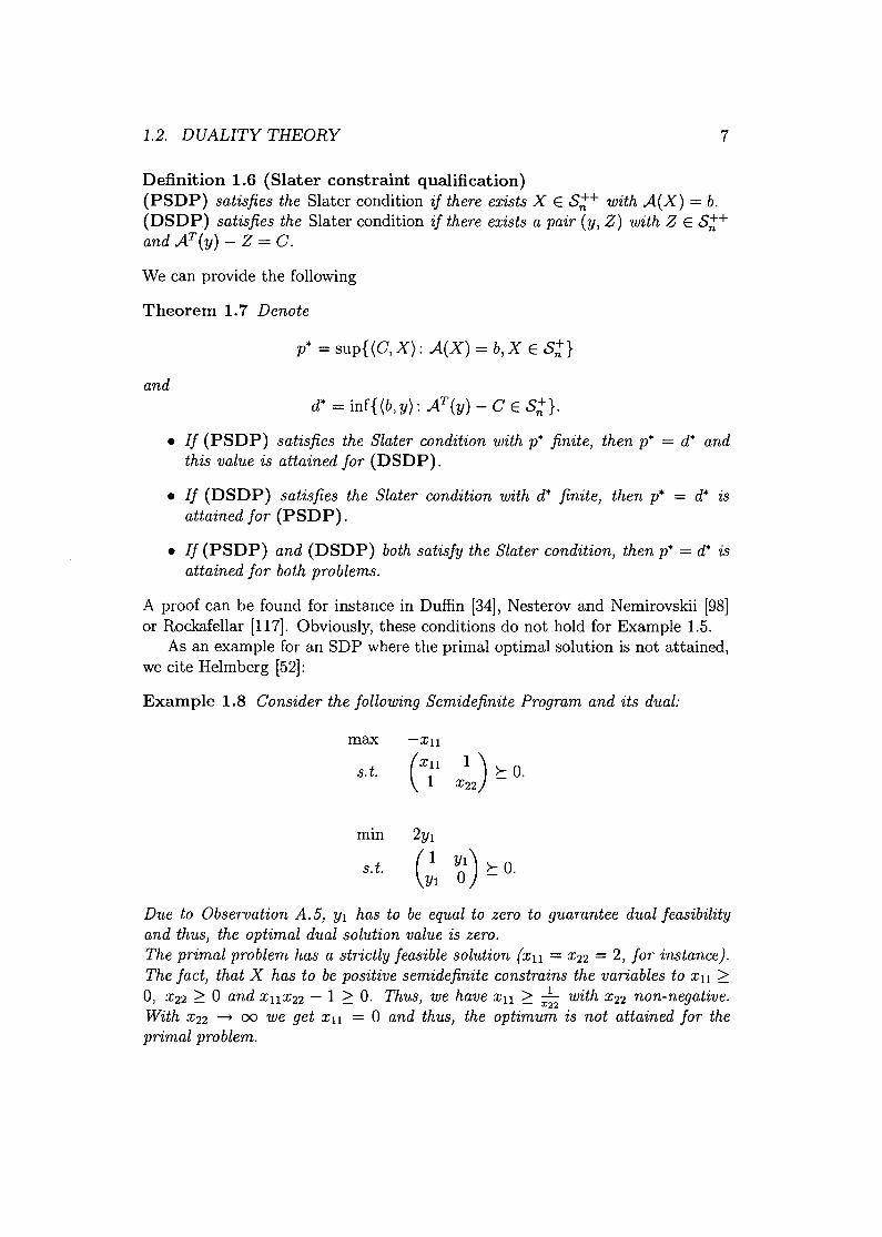
As an example for an SDP where the primal optimal solution is not attained,we cite Helmberg [52]:
Example 1.8 Consider the following Semidefinite Program and its dual:
max -Xll
S. t. (X;1 1 ) ta.X22
mm 2Yl
s.t. (:1 ~) ta.
Due to Observation A. 5, YI has to be equal to zero to guarantee dual feasibilityand thus, the optimal dual solution value is zero.The primal problem has a strictly feasible solution (Xll = X22 = 2, for instance).The fact, that X has to be positive semidefinite constrains the variables to Xll ~
0, X22 ~ a and XllX22 - 1 ~ O. Thus, we have Xll ~ X~2 with X22 non-negative.With X22 -. 00 we get Xll = a and thus, the optimum is not attained for theprimal problem.
8 CHAPTER 1. SEMIDEFINITE PROGRAMMING
We have seen in (lA) that a zero duality gap implies (Z,X) = 0 and hence,ZX = 0 (due to Lemma AA). This motivates the following
Definition 1.9 (Complementary slackness) Matrices X E s;t and Z E s;tare complementary if ZX = O.
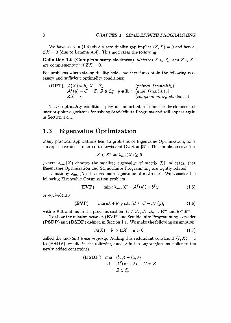
For problems where strong duality holds, we therefore obtain the following nec-essary and sufficient optimality conditions:
(OPT) A(X) = b, X E s;t (primal feasibility)AT(y) - C = Z, Z E s;t, Y E IRm (dual feasibility)ZX = 0 (complementary slackness)
These optimality conditions play an important role for the development ofinterior-point algorithms for solving Semidefinite Programs and will appear againin Section lA.l.
1.3 Eigenvalue OptimizationMany practical applications lead to problems of Eigenvalue Optimization, for asurvey the reader is referred to Lewis and Overton [85]. The simple observation
X E s;t {::}Àmin(X) ~ 0
(where Àmin(X) denotes the smallest eigenvalue of matrix X) indicates, thatEigenvalue Optimization and Semidefinite Programming are tightly related.
Denote by Àmax(X) the maximum eigenvalue of matrix X. We consider thefollowing Eigenvalue Optimization problem
or equivalently
(EVP)
(EVP)
(1.5)
(1.6)
with a E IR and, as in the previous section, C E Sn, A: Sn -+ IRm and b E IRm.To show the relation between (EVP) and Semidefinite Programming, consider
(PSDP) and (DSDP) defined in Section 1.1. We make the following assumption:
A(X) = b =? trX = a > 0, (1.7)
called the constant trace property. Adding this redundant constraint (I, X) = ato (PSDP), results in the following dual (À is the Lagrangian multiplier to thenewly added constraint)
(DSDP') mm (b, y) + (a, À)S.t. AT(y) + ÀI - C = Z
ZES;t.

1.3. EIGENVALUE OPTIMIZATION
Assuming that strong duality holds for the underlying problem, we have
(Z, X) = 0, Z E S;;, XES;;
at the optimum and due to Lemma A.4 follows
ZX=o.
9
Therefore the optimal Z is singular (if Z would be non-singular, we obtain X = 0which contradicts trX > 0) and all eigenvalues of -Z must be non-positive withat least one eigenvalue equal to zero. Hence,
Àmax(-Z) = 0 {::} Àmax(C- AT(y) - ÀI) = 0{::} Àmax(C- AT(y)) - À = 0{::} À = Àmax(C- AT(y)).
Substituting for À in the objective function of (DSDP'), we obtain
which is (EVP).For easier notation, define
(1.8)
to be the function to be minimized. (To simplify matters, we assume multipliera to be equal to one.) Due to the well-known fact
Àmax{X)= max{ (W, X): trW = 1, WES;;}
we can rewrite (1.8) as
f(y) - max{ (C - AT(y), W) + bTy: trW = 1, WES;;} =
max{ (C, W) + (b - A(W)f y: trW = 1, WES;;}.
(1.9)
Recall that function Àmax(.) is differentiable if and only if the maximal eigenvaluehas multiplicity one. Typically, the largest eigenvalue has multiplicity larger thanone for eigenvalue optimization problems and therefore one has to deal with thesub-differential of Àmaxat X,
OÀmax(X) = {W ES;;: (W,X) = Àmax(X), trW = I}
(confer for instance Overton [100]). For function (1.8) we then get
of(y) = {b - A(W): (W, C - AT(y)) ,=Àmax(C- AT(y)), trW = 1, WES;;}
10 CHAPTER 1. SEMIDEFINITE PROGRAMMING
(1.10)
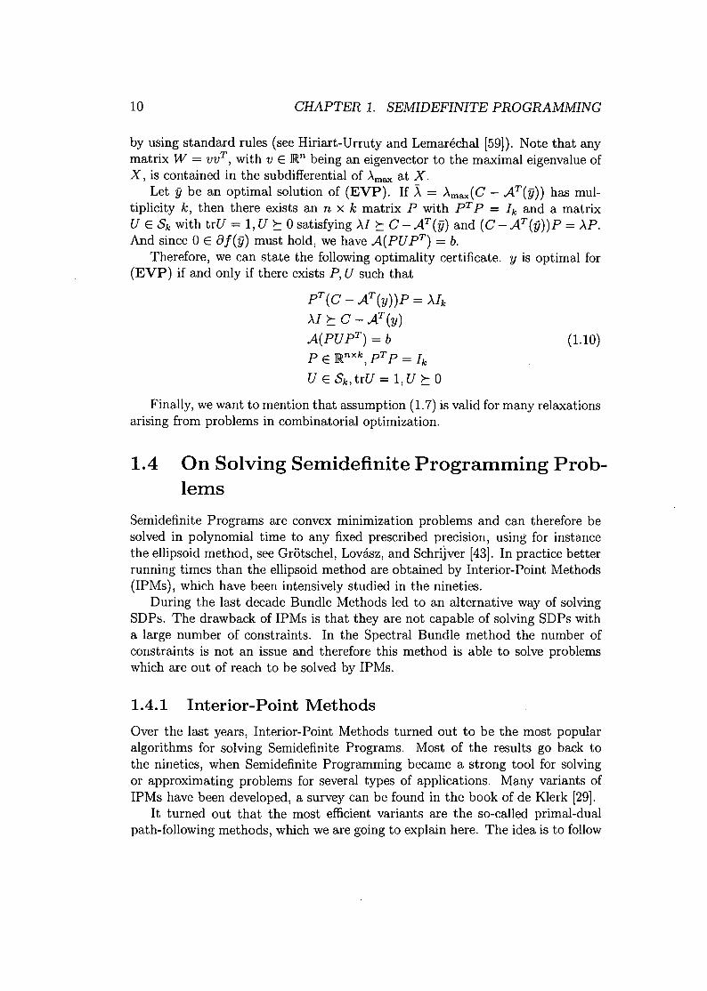
by using standard rules (see Hiriart-Urruty and Lemaréchal [59]). Note that anymatrix W = vvT, with v E !Rn being an eigenvector to the maximal eigenvalue ofX, is contained in the subdifferential of Àmaxat X.
Let y be an optimal solution of (EVP). If >. = Àmax(C - AT(y)) has mul-tiplicity k, then there exists an n x k matrix P with pT P = h and a matrixU E Sk with trU = 1,Ut 0 satisfying ÀI t C-AT(y) and (C-AT(y))P = ÀP.And since 0 E ôf(y) must hold, we have A(PU PT) = b.
Therefore, we can state the following optimality certificate. y is optimal for(EVP) if and only if there exists P, U such that
pT(C - AT(y))p = ÀhÀI t C - AT(y)A(PUpT) = bp E !Rnxk, pT p = hU E Sk, trU = 1,Ut 0
Finally, wewant to mention that assumption (1.7) is valid for many relaxationsarising from problems in combinatorial optimization.
1.4 On Solving Semidefinite Programming Prob-lems
Semidefinite Programs are convex minimization problems and can therefore besolved in polynomial time to any fixed prescribed precision, using for instancethe ellipsoid method, see GrätscheI, Lov8.sz,and SchriJver [43]. In practice betterrunning times than the ellipsoid method are obtained by Interior-Point Methods(IPMs), which have been intensively studied in the nineties.
During the last decade Bundle Methods led to an alternative way of solvingSDPs. The drawback of IPMs is that they are not capable of solving SDPs witha large number of constraints. In the Spectral Bundle method the number ofconstraints is not an issue and therefore this method is able to solve problemswhich are out of reach to be solved by IPMs.
1.4.1 Interior-Point MethodsOver the last years, Interior-Point Methods turned out to be the most popularalgorithms for solving Semidefinite Programs. Most of the results go back tothe nineties, when Semidefinite Programming became a strong tool for solvingor approximating problems for several types of applications. Many variants ofIPMs have been developed, a survey can be found in the book of de Klerk [29].
It turned out that the most efficient variants are the so-called primal-dualpath-following methods, which we are going to explain here. The idea is to follow
1.4. ON SOLVING SEMIDEFINITE PROGRAMMING PROBLEMS 11
approximately a central path in the interior of the feasible region to reach theoptimum. This central path is obtained by replacing the optimality conditionsby "nearly" optimality conditions.
Throughout this section we make the following
Assumption 1.10 The Slater constraint qualification holds for (PSDP) and(DSDP).
Let us recall the necessary and sufficient optimality conditions for (PSDP)and (DSDP).
(OPT) A(X) = b, X E S;i (primal feasibility)AT(y) - C = Z, Z E S;i, Y E]Rm (dual feasibility)ZX = 0 (complementary slackness)
The idea is to replace the last condition by
ZX = Ji'!
with J-L> 0 and let J-L~ O. In order to derive this perturbed system, we definethe following auxiliary problem.
(PSDP,J mm (C,X) - J-Llogdet(X)s.t. A(X) = b
XE S;+.
J-L> 0 is the so-called barrier parameter and -log det(X) the barrier function.Dualizing the equality constraints, we get the Lagrangian
LJ1-(X,y) = (C,X) - J-Llogdet(X) + (y,b- A(X» (1.11)
and compute the gradients with respect to X and y, respectively, in order toderive the KKT-conditions, necessary for optimality.
C - J-LX-I - AT(y)= b-A(X).
(Note that \7xlogdet(X) = X-I.) Setting the gradients equal to zero, we get
(OPTJ1-) A(X) = b, X E S;i+AT(y)+Z=C, ZES;i+, yE]Rm
XZ = J-LI.
Theorem 1.11 Under Assumption 1.10, (OPTJ1-) has for all J-L> 0 a uniquesolution (X(J-L), Y(J-L),Z(J-L».
12 CHAPTER 1: SEMIDEFINITE PROGRAMMING
A proof can be found for instance in Nesterov and Nemirovskii [98],Vandenbergheand Boyd [126]or Monteiro and Todd [96]. We define
Definition 1.12 (central path) The smooth curve {(X(!L),Y(f-L),Z(!L)):!L >O} is called the primal-dual central path.
Let ç = (X, y, Z), X E S:+, Z E S:+ be any point, not necessarily lying onthe central path. The goal is, to find ßç = (ßX, ßy, ßZ), such that ç + ßçcomes closer to the central path and iterate with smaller !L until f-Lis sufficientlysmall (i.e. !L ---+ 0).
The system to be solved in order to find the appropriate ßç, that would bringthe current point on the central path is:
A(X + ßX) = bAT(y + ßy) - C = Z + ßZ(X + ßX)(Z + ßZ) =!LI
(1.12)
This system has m + n(nz+l) + nZ equations in 2n(nz+l) + m variables. Due to thefact that the product of two symmetric matrices is not symmetric in general, thissystem of equations is overdetermined and we cannot apply the Newton methodto solve it. Many variations of system 1.12 have been proposed, to fix this andto obtain reasonable search directions. Before explaining one of these searchdirections, we sketch a generic primal-dual path-following algorithm.
Algorithm 1.13 (generic primal-dual interior-point algorithm) see Mon-teiro and Todd (96)
Input.ça := (Xa, Ya,Za), Xa E S:+, Za E S:+, é > O.
Initialization.!La := (Xa, Za) In.k:= O.
while !Lk > é or IIA(Xk - b)lloo > é or IIAT(Yk) - C - Zklloo > édetermine a search direction ßÇk from a linearized model of 1.12 for
!L = akf-Lk,ak E [0,1], such that ßXk and ßZk are symmetric.Çk+l := Çk + CikßÇk where Cik> 0 is chosen, such that
Xk+1 E S:+ and Zk+l E S:+.!Lk+l = (Xk+1, Zk+l) In.k := k + 1.
end
About twenty different search directions have been reviewed by Todd [123].We will use the HKM-direction, that was developed independently by Helmberg,

1.4. ON SOLVING SEMIDEFINITE PROGRAMMING PROBLEMS 13
Rendl, Vanderbei, and Wolkowicz [56], Kojima, Shindoh, and Rara [74] andMonteiro [95]. They solve the following system to obtain a search direction:
A(~X) = b - A(X)AT(~y) - ~Z = z +0 - AT(y)Z~X +~ZX = I-'J - ZX
(1.13)
These equations are solved for (~X, ~y, ~Z) and then ~X is symmetrized. Al-though this idea seems quite simple, it is computationally very efficient. Theo-retical convergence analysis shows, that for small E > 0 and appropriately chosenJ-L, in each iteration the full step yields a feasible solution. Moreover, a primaland dual feasible solution pair (X, y) with duality gap less than E can be foundafter O(J1ïllogEI) iterations (see Monteiro and Todd [96]).
1.4.2 Spectral Bundle MethodIn Section 1.3 we have shown the relation between Eigenvalue Optimization andSemidefinite Programming. ReImberg and Rendl [55]developed the Spectral Bun-dle Method, a machinery to solve problem (EVP) and therefore, use this as analternative to Interior-Point Methods for solving SDPs. Interior-Point Methodsfail for SDPs with a large number m of constraints, since in every iteration asystem of order m has to be solved. For these problems the Spectral BundleMethod may still obtain solutions in reasonable time. We explain the algorithmfollowing [55] and [51].
Recall, that in Section 1.3 we introduced
(1.14)
the function to be minimized. Two ingredients are used to minimize this function:the bundle concept and the proximal point idea. To apply the bundle method, weneed to have a function Î, approximating f in the neighborhood of the currentiterate. Introduce
L(W, y) := (0 - AT(y), W) + bTy.
With (1.9) we can now rewrite f(y) as
f(y) = max{L(W,y): WE s;t, trW = I}.
Replacing the feasible region {W: W E s;t, trW = I} by a subset that is com-putationally more efficient to handle, we have a minorant on f, that is easier tohandle than f itself. The proposed subset is
W = {aW +PVpT: a+trV = l,a 2: 0, V ES:}, (1.15)
where k is the number of columns in P and hence
Î(y) := max{L(W, y): W E W}. (1.16)
14 CHAPTER 1. SEMIDEFINITE PROGRAMMING
P is constructed in a way, that it contains subgradient information of the currentiterate, but keeping r, the maximum number of columns in P, small for compu-tational simplicity. (Note that parameter r controls the dimension of V.) To beable of using more information without increasing r, W is used as an aggregatesubgradient. Before going into detail concerning the construction of P and W,we explain the second ingredient of the Spectral Bundle Method, namely theproximal point idea.
Due to the fact, that we deal with an approximation of f which is reliableonly in the neighborhood of the current iterate, one has to penalize displacementfrom the current point, which results in
(1.17)
where u > 0 is the penalty parameter. Concerning this parameter, Helmberg andRendl [55]state the following
Remark 1.14 The choice of the weight u is somewhat of an art. There areseveral clever update strategies published in the literature, see for instance Kiwiel[71}, Schramm and Zowe [118}.
An iteration of the Spectral Bundle Method consists now in finding a new trialpoint Ynew and depending on how much progress is made at this point, we do aserious step or a null step. To keep notation simple, we skip the iteration counterin the subsequent description of an iteration of the Spectral Bundle Method. Letfi denote the current iterate. Ynew is obtained as the minimizer of (1.17), where jis the minorant on f in the current iteration. This minimizer is obtained by firstsolving
ma~ (0 - AT(fi), W) + bTfi - 21 (A(W) - b, A(W) - b)WEW U
(1.18)
by an Interior-Point Algorithm (see Section 1.4.1) and from this we get Wnew =a*W + PV* pT. The new iterate can then be easily computed by
Ynew = fi + ~(A(Wnew) - b).u
(1.19)
If this new iterate shows significant progress on finding the optimum, we makea serious step and the current iterate becomes Ynew' Otherwise a null step ismade, Le. the current iterate does not change, but information obtained duringthis iteration is used to improve the model.
Updating matrix P is done as follows. As long as P does not contain rcolumns, orthogonalize the new eigenvector with respect to P and add it as anew column. If the maximum number of columns in P is attained, we exploitthe information available in a* and V*, being the maximizers of this iteration.Let QAQT be the eigenvalue decomposition of V* and Q = [QI,Q2], with QI
1.4. ON SOLVING SEMIDEFINITE PROGRAMMING PROBLEMS 15
containing the eigenvectors associated to the 'large' eigenvalues of V*. Thus wecan rewrite the current maximizer
(1.20)
(1.21)
Then Pnew is computed such that it contains PQI and at least one eigenvectorto the current maximal eigenvalue of C - AT(Ynew), i.e. Pnew is an orthonormalbasis of [PQI vnew]. The remaining information contained in Q2 is included inthe new aggregate matrix W new by computing
1 - TWnew = A (a*W + PQ2A2(PQ2) ).
a* + tr 2
~ this way it is ensured, that the new aggregate matrix W new is contained inWnew.
We now have derived the necessary formulas for giving the formal descriptionof the algorithm.
Algorithm 1.15 (Spectral Bundle Method) Helmberg and Rendl [55}
Input.yo E]Rm and eigenvector Vo to Àmax(C - AT(yO))'ê > 0, improvement parameter mL E (0, ~).weight u > 0, upper bound R ~ 1 on the number of columns of P.
Initialization.k = 0, Xo = Yo, Po = Vo, Wo = vo(vof.
Iteration.1. (Direction finding.) Solve (1.18) and obtain Yk+I from (1.19).
Decompose V* into V* = QIAIQf + Q2A2QI with rank(QI) ~ R - 1.Compute Wk+I using (1.21).
2. (Evaluation.) Compute Àmax(C - AT(Yk+1)) and an eigenvector Vk+I'Compute Pk+I by taking an orthonormal basis of PkQI Vk+l'
3. (Termination.) If f(xk) - A(Yk+d ~ ê then stop.4. (Serious step.) If f(Yk+d ~ f(xk) - mL(J(xk) - lk(Yk+I)) then
set Xk+I = Yk+l and go to step 6.Otherwise continue with step 5.
5. (Null step.) Set Xk+1 = Xk.6. Increase k by 1 and go to Step 1.
For the proof of convergence the reader is referred to Helmberg and Rendl [55]. Aset of test graphs together with computational results for the Max-Cut relaxationand the Lov8.sz 'l9-function (see Section 2.2) are provided in their paper. Forthese instances the Spectral Bundle Method is by far superior than Interior-PointAlgorithms.
16 CHAPTER 1. SEMIDEFINITE PROGRAMMING
1.4.3 Software for Solving Semidefinite ProgramsInterior-Point Algorithms, as well as the Spectral Bundle Method have been im-plemented as open source software. Some of the Interior-Point Codes are runningunder Matlab, for instance SeDuMi (Sturm [122]), or SDPT3 (Toh, Todd, andTütüncü [125]), whereas e.g. CSDP by Borchers [24] is a C-code. The imple-mentation of the Spectral Bundle Method is SBMethod (Helmberg) . A list oflinks to the various packages can be found on the Semidefinite ProgrammingWebsite maintained by Helmberg [49]. Mittelmann [94] runs a website, providingbenchmarks for many SDP-solvers.
Chapter 2
Combinatorial Optimization
As the name reveals, in Combinatorial Optimization one wants to find an elementout of a set of combinatorial objects that is the optimizer for some given objectivefunction. More specifically, we have the following setting .
• A finite set E = {el, ... , en},
• a weight function w: E ---t Z, w( ei) being the weight of ei,
• a finite family F = {FI' ... ' Fm}, Fi ç E (feasible solutions),
• a cost function f : F ---t Z, f (F) = L:eEF w( e) (additive cost function),
• a problemopt{f(F): FE F},
where 'opt' is replaced by either 'min' or 'max'.
Usually, such problems can be formulated as Integer Programs with binary vari-ables, which indicate for each member of the collection, whether it belongs to thesubset or not.
A lot of problems fit into this definition. For example partitioning, assignment,covering, scheduling, shortest path, travelling salesman, spanning tree, matching,etc.
Before the year 1950, problems of this kind were studied independently ofeach other, for a historical survey see Schrijver [120]. Then Linear and IntegerProgramming became a unifying research topic and thus relations between theseproblems were found and exploited.
Over the past years new technologies in various areas like telecommunications,VLSI-design, production planning, etc. became more rapidly changing. Combina-torial Optimization turned out to appear in all of these applications and thus theresearch interest grew, since knowledge about problem properties and solutionalgorithms led to a competitive advantage.
17
18 CHAPTER 2. COMBINATORIAL OPTIMIZATION
Many textbooks on Combinatorial Optimization appeared during the lastyears, for a comprehensive collection on this subject we refer to Schrijver [119].Some Combinatorial Optimization problems that are of special interest in thecontext of Semidefinite Programing are explained in this chapter.
2.1 The Max-Cut ProblemLet G = (V(G), E(G)) denote an edge-weighted undirected graph with vertex setV(G) = {I, ... ,n} and m edges in the edge set E(G). Let We denote the weightof edge e = [ij], meaning edge e E E (G) links vertices i, j E V (G). The Max-Cut(MC) problem consists in finding a partition of the set of vertices into two partsso as to maximize the sum of the weights of the edges that have one end-node ineach part of the partition.
Let 8 be a subset of V. We denote a cut by
ö(8) := {e E E(G): e = [ij], 18n {i,j}1 = I},
hence Ö(8) contains all edges having exactly one end-node in 8, which are theedges linking 8 and V(G)\8.
w(T):= 2:WeeET
is the sum of the weights on edges in T ç E( G) and therefore the value of the cutgiven by ö(8) is given by w(ö(8)) and the Max-Cut problem can be formulatedas
(MC) max w(ö(8))s.t. 8 ç V(G).
Following the general formulation of a Combinatorial Optimization problem above,set E equals the set of edges E(G), and :F is the set of all cuts of G. The costfunction is the sum of the weights on the edges that form the cut and the objectiveis to maximize these costs.
The Max-Cut problem is known to be NP-complete and is one of the problemson the original list of NP-complete problems, investigated by Karp [66]. It is notonly of highly theoretical interest, but arises also in many contexts and thereforehas been well-studied over the last years. Goemans and Williamson [39]show thatthe ratio between the optimal cut value and the solution value of the basic SDPrelaxation of Max-Cut (MCSDP) (see Section 3.3.2), is at least 0.878 providedthere are non-negative weights on the edges. Note, that Hastad [48] showed thatit is NP-complete to approximate the Max-Cut problem with a factor bigger than0.9412.
Various heuristics for finding good solutions, and relaxations for getting tightupper bounds have been developed. We will review some of them in Chapter 3.

2.2. THE STABLE SET PROBLEM
2.2 The Stable Set Problem
19
A stable set or independent set in a given graph G = (V( G), E( G)) is a subsetI of V(G) such that no two vertices in I are adjacent. The maximum stable setproblem is the problem of finding a stable set of maximum cardinality. This max-imum cardinality is usually referred to as the stability number or independencenumber of a graph and denoted bya(G).
a(G) = max{III: I ç V(G), [ij] ~ E(G) Vi,j EI}. (2.1)
The stable set problem is closely related to two other problems, namely themaximum clique problem and the coloring problem.
A clique in a graph is defined as a subset Q of V( G) such that all vertices inQ are joint by an edge e E E(G). The maximum clique problem is therefore theproblem of finding a clique with maximum cardinality, denoted by weG),
weG) = max{IQI: Q ç V(G), [ij] E E(G) Vi,j E Q}. (2.2)
With G = (V (G), E( G)) being the complementary graph of G = (V (G), E( G)),it is easy to observe that
a(G) = weG).
A coloring of a graph G = (V(G), E(G)) is a mapping ß: V(G) -+ {I, ... ,k},where {I, ... , k} is the set of "colors" used, such that no two adjacent verticesare assigned the same color. The minimum k is the so-called chromatic numberand is denoted by xC G),
x(G) = min{k: ß(i) =1= ß(j) for i,j E V(G) and [ij] E E(G)}. (2.3)
Since within a clique every vertex needs to be colored differently, we get thefollowing inequality:
weG) ~ x(G).
This inequality can be strict, for instance consider C5, a cycle with IVI = 5.(w(C5) = 2 and X(C5) = 3.)
A graph is said to be perfect, if w( G') = x( G') for all induced subgraphs G'of G. This definition has been introduced by Berge, who also conjectured, thata graph is perfect if and only if it does not contain an odd cycle of length ~ 5 orits complement as an induced subgraph (Berge [20], [21]). This conjecture wasproved recently by Chudnovsky, Robertson, Seymour, and Thomas [28].
LOV8sZ [88]introduced the 'I9-numberof a graph. This number is the optimumof a semidefinite program and has the following property
a(G) ~ 'I9(G) ~ X(G). (2.4)
20 CHAPTER 2. COMBINATORIAL OPTIMIZATION
To compute the t9-number, the SDP to be solved is:
(THETA) t9(G) = max eTXeS.t. tr(X) = 1
Xij = 0 for i =1= j, [ij] E E( G)XE S;i,
e being the vector of all ones. (For equivalent definitions see Grätschel et al. [43]and Knuth [72].)The dual to (THETA) reads
(DTHETA) mm tS.t. tI + L:ijEE(G) )"ijEij - J E S;i,
where J = eeT.
The problem of deciding for a given integer k, whether a( G) :::::k or x( G) :::;kis NP-complete (Karp [66]). Moreover, Lund and Yannakakis [90] show that thereis a constant é > 0 such that no polynomial time algorithm exists that can achieveratio ne for the coloring problem unless P=NP. For the stable set problem Arora,Lund, Motwani, Sudan, and Szegedy [6]show the existence of a constant é > 0 forwhich there is no polynomial time algorithm that can find a stable set in a graph Gofsize at least n-ea(G) unless P=NP. On the positive side, Karger, Motwani, andSudan [64] use Semidefinite Programming for coloring a k-colorable graph withmaximum degree ~ with O(~I-2/ky'log~logn) or O(nI-3/(k+I)y'logn) colors.
The fact that the t9-number can be computed in polynomial time and that itsatisfies the 'sandwich' inequalities (2.4) makes it valuable for many applications.For perfect graphs it leads to the fact, that the maximum stable set problemand the coloring problem can be solved in polynomial time, since equality for thechromatic number and the clique number holds on these instances. For generalgraphs the gap between t9(G) and a(G) can be arbitrarily large. However, Alanand Kahale [2] state positive results about approximating a( G) via the t9-number.
2.3 The Graph Partitioning ProblemA problem related to Max-Cut is the graph partitioning problem. Again, we havea graph G = (V(G), E(G)), IV(G)I = n, and edge-weights We, e E E(G). Fur-thermore, numbers k and ml :::::m2 :::::... :::::mk are given, such that L:~=Imi = n.We now like to find a partition of V(G) into VI, V2, ..• , Vk and lVii = mi, i E{I, ... , k}, with a minimum total sum of the weights on the edges that are cut:
(GP) min L:I:Ss<t~kL:iEVs,jEVi W[ij]' (2.5)
This problem plays a major role in circuit design, for detailed applications we referto Lengauer [84]. In the special case of k = 2 and ml = m2 = n/2, the problem iscalled the bisection problem. If there are no constraints on the cardinality of the
2.3. THE GRAPH PARTITIONING PROBLEM 21
subsets, than for k = 2 and maximizing the sum of the weights on the cut-edges,we obtain the Max-Cut problem, see Section 2.1.
Let the columns of matrix X E {o,l}nxk, X = (Xij), be the characteristicvectors of the sets of the partition, i.e.
{I if i E Vj
Xij = 0 otherwise.
In order that each vertex i E V (G) is in exactly one set Vj, condition
must be valid. (ek, en being the vectors of all ones of size k and n, respectively.)Furthermore, to ensure that mi vertices are in the set Yi, the constraint
m = (ml, m2, ... , mk)T, must be fulfilled.Let A = (aij) be the adjacency matrix of the underlying graph. The value
1 1-trAXXT = -trXT AX2 2
gives the sum of the weights on all edges that are not cut and therefore the weightof the edges that are cut by this partition can be computed as
1_(eT Ae - trXT AX).2
With L = Diag(Ae) - A being the Laplace matrix of the graph and the equality
trXTDiag(Ae)X = eTAe,
we can formulate problem (GP) as follows.
(GP) mm trXTLXs.t. Xek = en
XTen = mX E {O, l}nxk.
(2.6)
Barnes and Hoffman [15] and Donath and Hoffman [33] developed eigenvaluebased relaxations for this problem. The problem is relaxed to containing onlythe constraint
XT X = Diag(m), XE ]Rnxk.
Through Theorem 2.1 Donath and Hoffman [33] obtain an eigenvalue basedbound.
22 CHAPTER 2. COMBINATORIAL OPTIMIZATION
Theorem 2.1 Let A and m be defined as above and set M := Diag(m). Then
Iw(uncut)1 ::;
Thus we get
1max{"2trXT AX: XTX = M}
11k
min{"2trMyT AY: yTy = h} ="2 LmjÀj(A).j=l
1 k
Iw(cut)1 ~ "2(eTAe - L mjÀj(A)) .. j=l
The proof can be found, for instance in Donath and Hoffman [33]or Rendl andWolkowicz [114].
Later on further SDP based bounds have been developed, confer Alizadeh [1],Rendl and Wolkowicz [114],Wolkowicz and Zhao [127], Karisch and Rendl [65].
Besides that, formulation (2.6) is similar to the Quadratic Assignment Prob-lem (QAP). The latest SDP relaxations oft he QAP are investigated in the paperof Rendl and Sotirov [112].
2.4 The Max-Sat ProblemIn order to explain the Maximum Satisfyability problem, we first need to intro-duce some notation. Xl, ... , Xn are Boolean variables and a literal z is either Xi
or Xi (the negation of Xi). A clause C of length k is the disjunctive combinationof k literals, i.e. C = Zl V ... V Zk, a weight Wc is assigned to each clause C.Clearly, clause C is satisfied, if at least one of the literals in the clause is assignedvalue 1. The Max-Sat problem consists in finding an assignment of values 0 and1 to the variables Xl, ... , Xn such that the total sum of the weights of satisfiedclauses is maximized. Given an integer k ~ 1, with the additional requirementthat each clause has length at most k, the problem is called Max-kSat.
Max-Sat and Max-kSat are known to be NP-hard. Hastad [48] showed thatthere is no (~ + é)-approximation for any é > 0, unless P=NP.
Johnson [62]constructed a ~-approximation algorithm for Max-Sat. A linearprogramming relaxation leads to the ~-approximation of Goemans and Williamson[38].
Via Semidefinite Programming, Goemans and Williamson [39]improved slightlytheir ~-approximation and obtained a 0.7554-approximation for Max-Sat.
Chapter 3
The Maximum Cut Problem
In this chapter we will take a closer look on one of the NP-complete combinatorialoptimization problems, the Max-Cut problem, already defined in Chapter 2. Wewant to state some of the important properties and give an overview on solutionmethods. It is easy to see, that the Max-Cut problem can be transformed toa quadratic (0-1) problem and vice versa. We explicate this transformation andpoint out an essential difference between Max-Cut problems and instances arisingfrom quadratic (0-1) problems.
3.1 Properties of the Max-Cut ProblemThe Max-Cut problem on a graph G = (V(G), E(G)), previously defined inSection 2.1, is given as
(MC) max w(<5(S))S.t. S ç V(G).
For several applications the following notation will be more convenient. LetV(G) := {I, ... ,n} be the vertex set of the given graph. The weights on theedges are expressed through the weighted adjacency matrix A = (aij), where
a .. = a .. = {We if e = [ij] E E(G)~J J~ a otherwise.
Given A, we introduce the Laplacian matrix L = (lij) associated to A, which isdefined as
n
lii =L aik, Vi E V(G)k=l
lij = -aij, i =1= j, i,j E V(G),
hence L = Diag(Ae) - A.
23
24 CHAPTER 3. THE MAXIMUM CUT PROBLEM
A vector X E {:l:l}n represents a cut in the graph in the sense that the sets{i : Xi = I} and {i : Xi = -I} form a partition of the vertex set of the graph, i.e.S = {i : Xi = I} and hence V\S = {i : Xi = -I}. It is easy to verify, that theweight of the cut given by S, can be computed as w(8(S)) = ~XT Lx:
n
XT Lx = L liiX; + 2 L lijXiXj =i=l l:5i<j:5nn n
L(Laik) + 2 L (-aij).l + 2 L (-aij). (-1) =i=l k=l [ij]~o(S) [ij]EO(S)
- 2 L aij + 2 L (-aij) + 2 L aij =[ij]EV(G) [ij]~O(S) [ij]EO(S)
- 4w(8(S)).
(Note that XiXj = -1 if [ij] E 8(S) and XiXj = 1 otherwise.) Hence, Max-Cut isequivalent to
(MC) max XT Lxs.t. xE {:l:l}n. (3.1)
(3.2)
Another way of specifying a cut is via its incidence vector, a vector indexed bythe edge set of the graph and defined as follows.
S {I if e E 8(S)Xe = 0 otherwise.
Let CUT denote the cut polytope, i.e. the convex hull of all incidence vectors ofcuts of graph G,
CUT = conv{xo(S): S ç V(G)}.
Thus, a third version of formulating the Max-Cut problem is given by the follow-ing linear program:
(MC) max wTys.t. y E CUT.
Many theoretical results of the cut polytope are elaborated in the book of Dezaand Laurent [32]. Barahona and Mahjoub [13] characterize the facet defininginequalities of the cut polytope and show different methods for constructing theseinequalities from known ones. Other papers dealing with the cut polytope arefor instance Barahona [10], Poljak and Thza [108], Poljak [105].
The Max-Cut problem is known to be NP-complete (Karp [66]) and it remainsNP-complete for some restricted versions, see Garey and Johnson [36]. However,several classes of graphs are known for which the solution can be obtained in poly-nomial time. To these classes belong graphs without long odd cycles (Grätscheland Nemhauser [41]), planar graphs (Hadlock [45],Orlova and Dorfman [99]), ormore generally graphs not contractible to K5 (Barahona [9]). More properties forcertain classes of graphs are surveyed in Poljak and Thza [109].
3.2. QUADRATIC (0-1) PROGRAMMING AND RELATION TO MC 25
3.2 Quadratic (0-1) Programming and its Rela-tion to Max-Cut
In this section we want to show, that solving a quadratic (0-1) problem andsolving a Max-Cut problem is essentially the same. Given a matrix Q of order nand a vector e, define the quadratic function
We consider the following unconstrained quadratic (0-1) program:
(QP) mm q(y)S.t. Y E {a, l}n.
(3.3)
(3.4)
This problem is equivalent to (MC), which has first been pointed out by Hammer[46]. The reduction from (QP) to (MC) has also been carried out in Barahona,Jünger, and Reinelt [14], a compact table of the transformation can be foundin Helmberg [50]. For completeness we show in detail in the subsequent twosubsections how to transform one problem into the other.
3.2.1 (QP)-+ (MC)
DefineW - ( a (Qe Q+cf)
- - (Qe + c)
and consider W to be the adjacency matrix of a graph with vertex set V{a, 1, ... ,n}. Then the Laplacian is given by
L Diag(We) - W =_ ( a (Qe + cf) _ ( eTQe + eTeo)
(Qe + c) Q a Diag(2Qe + c) .
Let X denote the incidence vector of a cut of this graph with value ~XT Lx. With-out loss of generality we can assume Xo = 1. Then, y defined as
1Yi = 2 (Xi + 1), 1::; i ::;n
is a vector in {a, l}n and therefore solution of (QP).The solution value of (MC) of the adjacency matrix W expressed in terms of
Y through the equality Xi = 2Yi - 1, 1::; i ::;n is the following:
26
Therefore,
CHAPTER 3. THE MAXIMUM CUT PROBLEM
(1 ) T ( 0 (Qe + C)T )
2y - e (( Qe + c) Q
- (q~) Diag(2~e + c) )) ( 2y ~ e ) =
_ ( 1 ) T ( 0 (Qe + cf) ( 1 )2y - e (Qe + c) Q 2y - e
(q(e) ) T ( 1 )
- Diag(Qe) + Diag(Qe + c) e =
- (0 + 4(Qe + C)Ty - 2q(e) + 4yTQy - 4eTQy + eTQe)-(q(e) + eTQe + q(e)) =
_ 4(yTQy + eT y - q(e)).
3.2.2 (MC)-+ (QP)Conversely, let be given a graph with node set V = {O,1, ... , n} and the (n +1) x (n + 1) Laplacian
L = (ln Lf2)L12 L22
where Ln is a n x n matrix. Let y be a solution of (QP) with Q = L22 and
c = L12 - L22e. Then, x = ( ~ ), Xo E IR, x E IRn defined as
Xo = 1, x = 2y - e
is a vector {::I:1}n+1 and therefore a solution of (MC). The value of the cutassociated to this solution, in terms of y is as follows:
q(y) -
-
-
-
-
-
yTQy + cTyyT LnY + (L12 - L22ef y
~(x + e)L22(x + e) + ~(L12 - L22e)T(x + e)4 2
~(XT L22XT + 2eT L22X + eT L22e) + ~(Lf2X + Lf2e - eT L22x - eT L22e)4 2
~(xT L22X + 2Lf2X + ln -ln - eT L22e + 2Lf2e)41_xT Lx - (ln - 2Lf2e + eT L22e).4
3.3. RELAXATIONS OF THE MAX-CUT PROBLEM 27
Therefore, -Lf2)Le.22
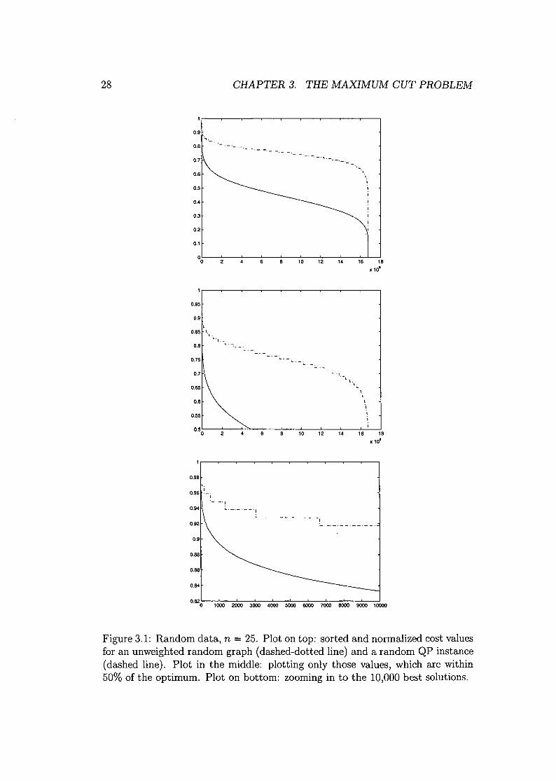
3.2.3 (MC) Ys. (QP)For all algorithms available, it turned out that solving instances of (MC) seemsto be a much harder job than solving instances arising from (QP). In order toinvestigate this behaviour, let us take a closer look on two random instances. Wegenerate an unweighted random graph with n = 25 vertices and edge-probability~. Also, we generate a random instance of (QP), where all entries in Q and carechosen from [-lOa, 100]. Due to the small size of these problems, we are able toenumerate all 224 solutions, and plot the sorted and normalized objective valuesin Figure 3.1.
The picture nicely shows that objective values of the (QP) instances are quiteevenly spread over the interval of possible values. Contrary, for (MC) the densityof cut values in the top quarter of the interval is clearly much higher than in theremaining part. For the (MC) instance, half of the solution values are within25% of the optimum, whereas for the (QP) instance only 0.5% are in that 25%regIOn.
It is evident that the optimal solution is much harder to identify when ten-thousands of solutions lie within a 5% interval of the optimum, as it is the caseof the (MC) instance, whereas for the (QP) instance only a few hundred arethat close. (The bottom-plot in Figure 3.1 shows for both problems the best10,000 objective values.) Therefore, solving problems originated from (MC) areobviously more challenging than (QP) problems.
3.3 Relaxations of the Max-Cut ProblemIn this section we recall the most popular relaxations of the Max-Cut problemtogether with some of the recent methods for solving it to optimality. We sketchthe algorithms and summarize their limits. A survey of techniques developedbefore 1980 can be found in Hansen [47].
3.3.1 Relaxations Based on Linear Programming
Consider the linear program (3.2). For a graph G = (V, E) define y E IRE asy(E) := LeEE Ye. The observation that any odd cycle intersects with a cut on aneven number of vertices motivates the construction ofthe odd cycle inequalities:
y(F) - y(C\F) ::; IFI- 1 for each cycle C ç E, F ç c, IFI odd. (3.5)
A special class of odd cycle inequalities are the triangle inequalities, which arisewhen C in (3.5) is a cycle of length three, i.e. a triangle. For F = C (hence
28 CHAPTER 3. THE MAXIMUM CUT PROBLEM
0.9 .,0.8
0.2
0.1
oo
0.95
0.9
2 10 12 14 16 18
x 10'
0.8
"
0.85 '\\.'r ._ .... _
0.75
0.7
0.98
'.0.96 '-. ,
"---',0.94
0.88
0.88
0.84
L. , -,,
"
"
,,10 12 14 16 18
x 10'
....-.--.- _.--. --'-1
0.82 o 1000 2000 3000 4000 5000 6000 7000 6000 9000 ooסס1
Figure 3.1: Random data, n = 25. Plot on top: sorted and normalized cost valuesfor an unweighted random graph (dashed-dotted line) and a random QP instance(dashed line). Plot in the middle: plotting only those values, which are within50% of the optimum. Plot on bottom: zooming in to the 10,000 best solutions.
3.3. RELAXATIONS OF THE MAX-GUT PROBLEM 29
(3.6)
IFI = 3), we get the inequality y(F) :::;2 and for FcC (IFI = 1) we obtainy(F) - y( C\F) :::;O. So, if C is formed by the edges [ij], [ik], Uk], we obtain
Yij + Yik + Yjk < 2Yij - Yik - Yjk < a
-Yij + Yik - Yjk < a-Yij - Yik + Yjk < a
The odd cycle inequalities and also the trivial inequalities a :::;Ye :::; 1,e E Eare all valid for any y E CUT (the cut polytope, see Section 3.1). Therefore,a linear programming relaxation of the Max-Cut problem can be derived byreplacing the constraint y E CUT in (3.2) by the odd cycle inequalities anda :::; Ye :::; 1, e E E. Nevertheless, this LP has then an exponential numberof inequalities and therefore an attempt of feeding this problem into some LPsolver might already fail when specifying all the constraints. On the other hand,Grätschei, LOV8sZ, and Schrijver [42]show that one can optimize a linear objectivefunction over a polytope in polynomial time if and only if one can solve theseparation problem for this polytope in polynomial time. Barahona and Mahjoub[13] give a polynomial time algorithm for separating the cycle inequalities andthus a cutting plane approach can be developed, where the LP relaxations canbe exploited by using the cycle-inequalities in an iterative algorithm.
Barahona et al. [14]designed such a cutting plane algorithm within a Branch& Bound framework that uses these inequalities. They solve in the root node thetrivial LP
max wTys.t. 0:::; Ye :::;1, e E E
and generate then cutting planes not only at the root, but also at each node ofthe Branch & Bound tree. They sketch the cutting plane procedure performedat each node as follows:
beginrepeat
solve LP;obtain lower bound;if successful then try to fix variables;try to generate cutting planes;revise LP;
until no cutting planes generated;if LP solution feasible
then backtrackelse branch
end
To obtain a lower bound (Le. finding a cut in the graph), a heuristic isapplied to the solution obtained by solving the LP. This heuristic computes a
30 CHAPTER 3. THE MAXIMUM CUT PROBLEM
maximum spanning tree in the original graph with edge weights lYe - ~ I (y E IRE isthe LP solution) and assigns the vertices to one ofthe two subsets of the partitionaccording to the weights on the edges of this tree. This yields a feasible solutionto the Max-Cut problem.
The lower bound serves for fathoming nodes in the Branch & Cut tree, butis also used for fixing variables. If Ye = a and ZLP - de < ZF, where ZLP is theobjective function value, dE IRE the reduced cost vector and ZF the value of thebest known cut in G, clearly we can fix the variable associated to this edge to O.Similarly, if Ye = 1 and ZLP + de < ZF, we can fix the variable to 1. Furthermore,edges, that belong to a subgraph induced through the edges fixed to a or 1, canbe fixed by logical implications.
Odd cycle inequalities are used to generate cutting planes. Several ideasare incorporated for finding violated odd cycle inequalities. Barahona et al. [14]proceed according to the followingorder, until violated inequalities are found:
1. Enumerate all 3-cycles.
2. Apply a coloring heuristic for finding violated odd-cycle inequalities. Thisheuristic guarantees, that in an integral solution, that is not a cut, violatedodd-cycle inequalities will be found.
3. Apply a spanning tree heuristic to detect violated odd-cycle inequalities.
4. Use exact separation (see Barahona and Mahjoub [13]).
Branching is done by choosing the variable Xe with fractional value closest to~, and among those one with maximum absolute objective function coefficient.
Recent results on a refinement of this LP based cutting plane algorithm aredue to Liers, Jünger, Reinelt, and Rinaldi [87]. They focus on solving toroidalgrid graphs arising from physical applications. Since these graphs are sparse, LPbased method are the proper tool for solving these instances.
Limits of this method: The computational results presented in Barahonaet al. [14]show that graphs of any density up to n = 30 nodes can be computedin reasonable time. But with an increasing number of nodes, the limits on thedensity of the graphs decreases rapidly. Graphs with n = 100 nodes can onlybe solved, if the edge density is at most 10%. The algorithm of Liers et al. [87]solves 3-dimensional toroidal grid graphs with Gaussian distributed weights ofsize 7 x 7 x 7 within minutes and 2-dimensional of size 20 x 20 within seconds.However, for dense instances also this algorithm is not practical.
3.3.2 A Basic SDP RelaxationConsider (MC) formulated as (3.1) and do a transformation of variables, namely
X:= XXT.

3.3. RELAXATIONS OF THE MAX-CUT PROBLEM 31
(3.7)
Hence X has the properties that it is positive semidefinite, it has rank one andall diagonal elements are equal to one. Furthermore, the value of a cut associatedto X can be computed as
111_xT Lx = -trLX = - (L X)4 4 4'.Thus an equivalent formulation of the Max-Cut problem is
(MC) max (L, X)s.t. diag(X) = e
rank(X) = 1X E sn, X ~ o.
A semidefinite relaxation can be obtained by simply dropping the rank-1 con-straint:
Its dual form
(MCSDP) max (L, X)s.t. diag(X) = e
X E sn, X ~ o.(3.8)
(3.9)
(3.10)
(MCDSDP) min eTus.t. Diag(u) - L ~ 0
was introduced by Delorme and Poljak [30] as the (equivalent) eigenvalue opti-mization problem
(MCEIG) mm n>'max(L - Diag(u))s.t. uTe = 0
u E ]Rn.
The primal version (MCSDP) can be found in Poljak and Rendl [107].The model (MCEIG) is used in Poljak and Rendl [106] as the bounding
routine in a Branch & Bound framework.
Limits of this method: This basic SDP bound can be computed rathercheaply by using for instance an Interior-Point algorithm. However, within aBranch & Bound scheme the progress of the bound at each node of the B&B treeis disappointingly small and therefore the number of nodes in this tree becomesrather large, already for medium sized problems. The maximum cut in graphsup to n = 50 nodes can be computed quite efficiently, but for larger n a solutionin reasonable time can only be obtained for instances where the initial gap isalready very small.
Further SDP based MC relaxations. This basic relaxation has been ex-ploited in various ways during the past decade. For example it can be strength-ened by the so-called hypermetric inequalities. Other relaxations of (MC) arisingfrom SDP are the so-called lift-and-project methods. A separate chapter is ded-icated to these SDP relaxations (Chapter 4).
32 CHAPTER 3. THE MAXIMUM CUT PROBLEM
3.3.3 Convex Quadratic Relaxations
Billionnet and Elloumi [23] came up with the idea of convexifying the objectivefunction and then using a Mixed-Integer Quadratic Programming (MIQP) solverfor solving problem (3.4). Their algorithm works in detail as follows. Considerproblem (QP) and define for any vector u E ]Rn the Lagrangian
n
qu(x) := q(x) +LUi(Xi - x~) = xT(Q - Diag(u))x + (c + U)T X.i=l
It is easy to see, that an equivalent problem to (QP) is
(QPu) mm qu(x)S.t. x E {O,l}n. (3.11)
Relaxing the integrality constraint in problem (QPu) gives the lower bound ß(u)on (QP),
ß(u) = min qu(x)s.t. 0::; Xi::; 1, i E {I, ... ,n}.
If the vector u is chosen, such that Q - Diag( u) is positive semidefinite, ß( u) isobtained by solving a convex quadratic problem, which can be done efficiently.Now, if u* is the maximizer of ß(u), the "optimal" lower bound ß* will be ob-tained, i.e.
ß* = ß(u*) = max{ß(u) : (Q - Diag(u)) ~ O,u E ]Rn}.
Billionnet and Elloumi [23] observe, that the çlual to this SDP coincides with thebasic Max-Cut relaxation (MCSDP), see Section 3.3.2.
The solution of problem (QP u) (or (QP u' ), respectively) can be derivedby using an MIQP solver, Le. a Branch & Bound algorithm using ß(u), thecontinuous relaxation of (QPu), as bound.
The computational effort for this algorithm can be summarized as follows:
• Preprocessing phase: solve an SDP to obtain a vector u* and a bound ß* .
• Use an MIQP solver for solving problem (QPu')' Even though the compu-tation of the bounds is very cheap, the number of nodes in the Branch &Bound tree typically exceeds 100,000 for problems of n = 100 variables, asreported in [23].
Limits of this method: Quadratic problems with some special structure canbe solved up to n = 100 variables. But the method is not capable of solvingcertain classes of Max-Cut instances of this size (for example, graphs with edgeweights chosen uniformly from {-I/O/I}).
3.3. RELAXATIONS OF THE MAX-CUT PROBLEM 33
3.3.4 Second-Order Cone Programming Relaxations
Kim and Kojima [68], and later on Muramatsu and Suzuki [97] use a second-order cone programming (SOCP) relaxation as bounding routine in a Branch &Bound framework to solve Max-Cut problems. Second-order cone programmingis a special case of symmetric cone-programming. The second-order cone Kn isdefined by
SOCP can be used to relax nonconvex quadratic problems. Muramatsu andSuzuki [97]propose an SOCP relaxation of (MC) that includes convex quadraticconstraints, which reflect the structure of the graph. They are able to incorporatethe triangle inequalities (see Section 3.3.1) to tighten the feasible region efficiently.
However, the basic SDP relaxation (see Section 3.3.2) performs better thantheir SOCP relaxation and the method works only for sparse graphs.
Limits of this method: The algorithm is capable of solving very sparse in-stances only. The largest graphs for which solutions are reported are randomgraphs (weights between 1 and 50) of n = 120 nodes and density 2%, and graphs,which are the union of two planer graphs up to n = 150,d = 2%.
3.3.5 Branch & Bound with Preprocessing
Pardalos and Rodgers [102], [103] solve the quadratic program by Branch &Bound using a preprocessing phase where they try to fix some of the variables.The function to be minimized is (3.3). The test on fixing the variables exploitsthe fact, that if x* is the global solution of
min{q(x) : x E 5}
(5 being a convex compact set), then x* is also optimal for the linear program
min{(V'q(x*)l x : x E 5}.
Limits of this method: Similar to the cutting plane technique in Barahonaet al. [14], dense instances up to n = 30 and sparse instances up to n = 100can be computed. Special classes of instances can be solved efficiently up ton = 200. These instances have off-diagonal elements in the range [0,100] anddiagonal elements lying in the fixed interval [-1,0], for the case I = 63 (thedensity is 100%). For other values of I, the problem may become much moredifficult to solve. However, the method fails forgeneral dense problems withn = 50 variables.
34 CHAPTER 3. THE MAXIMUM CUT PROBLEM
3.4 A Rounding Heuristic Based on SDPThe basic SDP relaxation (MCSDP) can be used to obtain a feasible solution ofthe Max-Cut problem, i.e. to generate a cut. This method is called the Goemans-Williamson hyperplane rounding technique [39] and works as follows. Let X =(Xij) be the optimal solution of (MCSDP). We have to find vectors VI,"" Vn,
Vi E jRk (for some k :S n), such that Xij = vT Vj' This can be done, by computingthe Cholesky Factorization VTV of X, with V E jRkxn. Some random vector r isthen used to set
8:={i:vTr~O} .
and obtain in this way a cut 6(8). This process can be iterated with varyingrandom vector r.
The cut obtained by this hyperplane rounding technique may be further im-proved by flipping single vertices. Also, instead of the solution matrix X of theSDP, a convex-combination of this matrix X with some cut-matrix XXT used tofind the Cholesky factorization may improve the result.
Summarizing, generating good cuts can be done iteratively in basically threesteps:
1. Apply the Goemans-Williamson hyperplane rounding technique to the pri-mal matrix X obtained from solving the (MCSDP). This gives a cut-vectorx.
2. The cut x is locally improved by checking all possible moves of a singlevertex to the opposite partition block.
3. Bring the rounding matrix towards a good cut by using a convex-combinationof X and xxT. With this new matrix go to 1. and repeat as long as onefinds better cuts.
Chapter 4
SDP Relaxations of the Max-CutProblem
In the previous chapter several properties and solution approaches of the Max-Cutproblem have been investigated and we gave a brief description of a basic semidef-inite relaxation. In this chapter we want to focus on models, that use SemidefiniteProgramming for obtaining upper bounds to this NP-complete problem.
4.1 The Basic RelaxationThe basic Max-Cut relaxation has already been derived in Section 3.3.2 as follows:
(MCSDP) max (L, X)s.t. diag(X) = e
X E sn, X t 0
and its dual form
(MCDSDP) mm eT us.t. Diag(u) - L t O.
We denote the feasible set of (MCSDP) as
En := {X E Sn: diag(X) = e, X tO},
(4.1)
(4.2)
(4.3)
called the elliptope. A study of this convex set can be found in Laurent andPoljak [78], [79].
As already mentioned in Section 2.1, for graphs with non-negative edge weights,the optimal solution of (MCSDP) is at most 14% above the value of the maxi-mum cut [39].
Several strategies have been applied for strengthening this SDP-based relax-ation. We will explore these methods in the subsequent sections.
35
36 CHAPTER 4. SDP RELAXATIONS OF THE MAX-CUT PROBLEM
4.2 Strengthening the Basic RelaxationIn Section 3.3.1 we introduced the odd-cycle inequalities, and as a special caseof it, the triangle inequalities, to strengthen the LP relaxation of the Max-Cutproblem.
Similar to the LP case, also the SDP bound can be improved by exploitingthe observation, that in any cycle of length three, exactly zero or two edges arecut. Considering matrix X = (Xij) representing a cut, the following inequalitiesmust be valid for all 1 :::;i < j < k :::;n:
Xij + Xik + Xjk > -1Xij - Xik - Xjk > -1
(4.4)-Xij + Xik - Xjk > -1-Xij - Xik + Xjk > -1
The polytope containing all matrices X E Sn with diag(X) = e and satisfyinginequalities (4.4), is called the metric polytope and denoted by MET.
MET :={X ESn: diag(X) = e, Xij + Xik + Xjk 2: -1,Xij - Xik - Xjk 2: -1, -Xij + Xik - Xjk 2: -1, (4.5)-Xij - Xik + Xjk 2: -I}.
This leads to the following relaxation, proposed in Poljak and Rendl [107]:
(SDPMET) I max (L, X)s.t. X EMET
X!: 0(4.6)
The number of inequalities of (SDPMET) is growing rapidly with increasing di-mension n. Including all these triangle inequalities and then solving the programby an Interior-Point Method (see Section 1.4.1)is intractable already for smalln. Computational results of solving this SDP with successively including the4(~) triangle inequalities can be found in Helmberg et al. [56]. Results are alsogiven in Rendl [111], where only a limited number of these triangle inequalitiesis considered.
A more general class of inequalities are the hypermetric inequalities, studiedin Deza and Laurent [31]. Let b be an integer vector with L:~=lbi is odd. Thisguarantees that
IxTbl 2: 1 for all X E {::I::l}n.
The following equivalences always hold:
And therefore the hypermetric inequalities must be valid for all matrices in thecut polytope.
4.3. LIFT-AND-PROJECT METHODS 37
The triangle inequalities can be derived as a special case of the hypermetricinequalities by setting for the triangle formed by the vertices i, j, k:
andbi=bj=l, bk=-l,bl=O, 'ïll~{i,j,k}.
Helmberg and Rendl [54] use the hypermetric inequalities as cutting planesand solve the SDP by an Interior-Point Code. At the initial step of the algorithmthey consider the basic semidefinite relaxation (4.1). Inequalities are added whilesolving the relaxation (i.e. after some Newton steps), as well as after the exactsolution to the relaxation has been obtained. Then the optimization processis restarted again. Later on, Helmberg [50] improved this algorithm by fixingvariables.
This algorithm has been used in a Branch & Bound framework. In Helmbergand Rendl [54] several branching rules are considered and discussed carefully.Although the relaxation produced very tight bounds, the results of the Branch& Bound code remained below the expectations of the authors. The number ofnodes in the Branch & Bound tree is very small, but the computation time pernode may be rather large. Most graphs up to n = 50 vertices can be solved inthe root-node of the Branch & Bound tree. Instances up to the size n = 100 canstill be solved, but the computational effort may be very high. Graphs with morethan 100 vertices are intractable for this algorithm.
4.3 Lift-and-Project MethodsSince the nineties several approaches have been developed to construct relaxationsto NP-hard problems by representing the polytope over which wewant to optimizeas the projection of another polytope lying in a higher dimensional space. Theycan be classified into the BCC method due to Balas, Ceria, and Cornuéjols [8],theSA method by Sherali and Adams [121], the LS method of Lovasz and Schrijver[89], and the method of Lasserre [76]. Details and relations about these lift-and-project methods can be found in the papers of Laurent [77]or Laurent and Rendl[80].
4.3.1 The Lifting of Anjos and Wolkowicz
Anjos and Wolkowicz [3] introduced an SDP relaxation for Max-Cut via a sec-ond lifting. They obtain the relaxation by adding redundant constraints to(MCSDP) and then use Lagrangian duality for deriving the dual of the dual.After a second lifting they end up with a relaxation called (SDP3), which is the
38 CHAPTER 4. SDP RELAXATIONS OF THE MAX-CUT PROBLEM
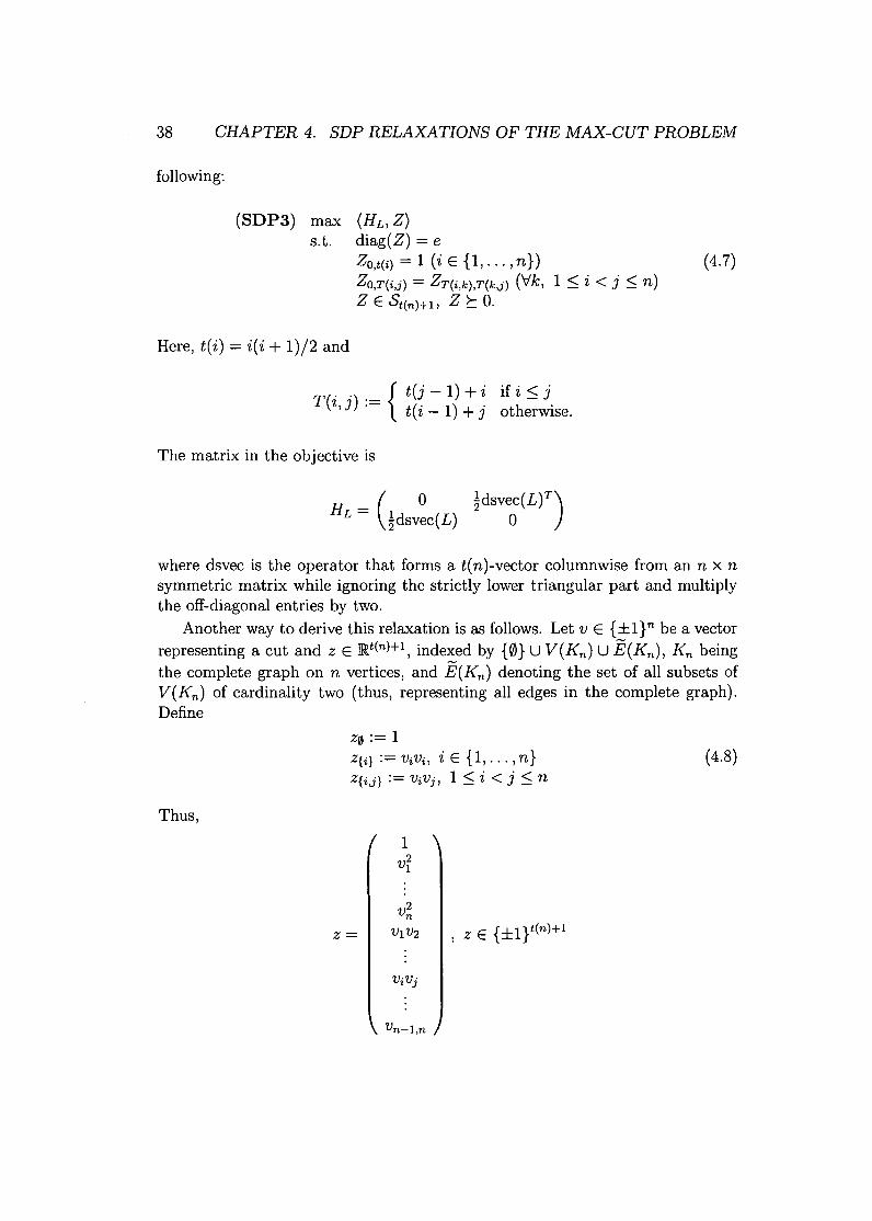
following:
(SDP3) max (HL, Z)s.t. diag( Z) = e
ZO,t(i) = 1 (i E {I, ... ,n}) (4.7)ZO,T(i,j) = ZT(i,k),T(k,j) (Vk, 1::;i < j ::; n)Z E St(n)+l, Z t O.
Here, t(i) = i(i + 1)/2 and
T(' .)._ { tU - 1) + i if i ::;j1" J.- t( i-I) + j otherwise.
The matrix in the objective is
H - ( 0 ~dSveoC(L)T)L - ~dsvec(L)
where dsvec is the operator that forms a t(n)-vector columnwise from an n x nsymmetric matrix while ignoring the strictly lower triangular part and multiplythe off-diagonal entries by two.
Another way to derive this relaxation is as follows. Let V E {::I::1}n be a vectorrepresenting a cut and z E jRt(n)+l, indexed by {0} U V(Kn) U E(Kn), Kn beingthe complete graph on n vertices, and E(Kn) denoting the set of all subsets ofV(Kn) of cardinality two (thus, representing all edges in the complete graph).Define
Thus,
z0:= 1Z{i} := ViVi, i E {I, ... ,n}Z{i,j} := ViVj, 1 ::;i < j ::; n
(4.8)
Z=
Vn-l,n
, Z E {::I::I }t(n)+l
4.3. LIFT-AND-PROJECT METHODS
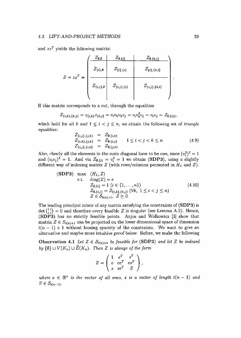
and zzT yields the following matrix:
39
Z{i,j},0
Z{i},{i}
Z{i,j},{i}
Z{i},{k,l}
Z{i,j},{k,l}
(4.10)
If this matrix corresponds to a cut, through the equalities
Z{i,k},{k,j} = Z{i,k}Z{k,j} = ViVkVkVj = ViV~Vj = ViVj = Z0,{ij},
which hold for all k and 1 ::; i < j ::;n, we obtain the following set of triangleequalities:
Z{i,j},{j,k} Z0,{i,k}Z{i,k},{j,k} Z0,{i,j} 1 ::; i < j < k ::;n (4.9)Z{i,j},{i,k} Z0,{j,k}
Also, clearly all the elements in the main diagonal have to be one, since (vi)2 = 1and (ViVj)2 = 1. And via Z0,{i} = vr = 1 we obtain (SDP3), using a slightlydifferent way of indexing matrix Z (with rows/columns permuted in HL and Z).
(SDP3) max (HL, Z)s.t. diag(Z) = e
Z0,{i} = 1 (i E {I, ... ,n})Z0,{i,j} = Z{i,k},{k,j} (Vk, 1::; i < j ::;n)Z E St(n)+l, Z t O.
The leading principal minor of any matrix satisfying the constraints of (SDP3) isdet G~)= 0 and therefore every feasible Z is singular (see Lemma A.2). Hence,(SDP3) has no strictly feasible points. Anjos and Wolkowicz [3] show thatmatrix Z E St(n)+l can be projected on the lower dimensional space of dimensiont(n - 1) + 1 without loosing sparsity of the constraints. We want to give analternative and maybe more intuitive proof below. Before, we make the following
Observation 4.1 Let Z E St(n)+l be feasible for (SDP3) and let Z be indexedby {0} U V(Kn) U E(Kn). Then Z is always of the form
where e E ]Rn is the vector of all ones, S is a vector of length t( n - 1) andS E St(n-l).

(4.11)
40 CHAPTER 4. SDP RELAXATIONS OF THE MAX-CUT PROBLEM
Proof: Consider any Z from the feasible set of (SDP3), with the following blockstructure:
Z = (~ U; ~:),s R S
with u E IRV(Kn), S E IRE(Kn). In order to prove the observation, we have to showthat
u = e, U = eeT, R = seT.
Because of the constraint ZO,{i} = 1, we have u = e.Then the leading 3 x 3 principal submatrix of Z reads
(~ ~ U~2)'1 U12 1
Since every principal minor of a positive semidefinite matrix has to be non-negative (see Theorem A.l) we get
U12 = 1.
Similarly we can derive, that any other Uij has to be equal to one if Z is positivesemidefinite, and thus we obtain U = eeT.
In the same way we get, for the principal submatrix formed by the rows/columns{0, {k}, {i,j}}
(1 1 S{i,j} )1 1 r{k},{i,j}
S{i,j} r{k},{i,j} 1
that r{k},{i,j} = S{i,j} must hold and therefore we end up with R = seT and wehave proved the observation. 0
Theorem 4.2 Let Y E St(n-l)+l be indexed by {0} U E(Kn), E(Kn) being thecollection of all the subsets of V(Kn) of cardinality two. (V(Kn) is the set ofvertices of the complete graph on n vertices.) Let QL be defined as
Q '= (~~~=lliiusvec(Lf)L . usvec(L) 0 '
where usvec(L) forms a vector columnwise from a symmetric matrix consideringonly the strictly upper triangular part of the matrix. Consider the following 3DP.
(SDP3p) max (QL, Y)s. t. diag(Y) = e
Y0,{i,j} = Y{i,k},{k,j} (Vk fJ. {i,j}, 1~ i < j ~n)
Y E St(n-l)+l, Y t O.
There is a bijection between the feasible sets of (SDP3) and (SDP3p).
4.3. LIFT-AND-PROJECT METHODS 41
Proof: Let F ç St(n)+l be the set of matrices feasible for (SDP3) and Fp çSt(n-l)+l the set of matrices feasible for (SDP3)p. Define f: F -t Fp, as
f(Z) = Z{0}UË(Kn)'
meaning that f(Z) is the prin~pal submatrix of Z, that contains only the rowsand columns indexed by {0}UE(Kn), hence we simply erase the columns indexedby V(Kn). (Note, that it is easy to verify that every Y in the image of f is feasiblefor (SDP3p ).)
Due to Observation 4.1, every matrix Y E Fp can be extended to a ZEFin a unique way. The fact that it is possible to extend Y to a feasible Z impliesthat f is surjective, and because of the fact, that this way of extending is unique,f is injective. Thus, f is a bijection between Fand Fp. 0
Anjos and Wolkowicz [3]prove that relaxation (SDP3p) lies in the elliptopeand satisfies all the triangle inequalities. Thus, the bound of this relaxation is atleast as good as the bound obtained by solving (SDPMET), which is already astrengthening of (MCSDP) (see Section 4.2). In fact they prove,
CUT ç F ç £ n MET
and show that these inclusions are strict for n 2: 5.They also present numerical results for graphs up to n = 12 vertices and
observe, that the (SDP3p) relaxation often yields the optimal value of (MC).Nevertheless, since the dimension of the matrix is (;) + 1 and the SDP has1+ G) + 3(;) linear equality constraints, it is out of reach to solve it for graphsof size n = 50.
4.3.2 The Lifting of Lasserre
Consider the general problem
max cTxs.t. Ax ~ b
xE {o,l}n
and denote
K:= {x E [0, It: Ax ~ b}, P:= conv({x E {a, l}n: Ax ~ b}).
(4.12)
Lasserre [76] constructs a hierarchy of semidefinite relaxations Qi of P with theproperty
42 CHAPTER 4. SDP RELAXATIONS OF THE MAX-CUT PROBLEM
The motivation for these relaxations comes from results about moment matrices.A detailed study and the proof of convergence can be found in Lasserre [76]orLaurent [77].
Applied to the Max-Cut problem, relaxation (Qo) coincides with the basicSDP relaxation (MCSDP). The relaxation (QI) is the following:
(QI) max (ML, Y)s.t. diag(Y) = e
Y0,{i,j} = Y{i,k},{k,j} (Vk fi. {i,j}, 1~ i < j ~n)Y{i,j},{h,k} = Y{i,h},{j,k} = Y{i,k},{j,h}
(for all distinct i, j, h, k E {I, ... , n})Y E S(~)+l' y?: o.
(4.13)
Clearly, this is a strengthening of (SDP3p), introduced in the previous section.The constraints additional to (SDP3p), we call them 4-cycle equalities, can alsobe motivated as follows. Consider y E lR(~)+l, with
Y0:= 1Y{i,j} := ViVj, 1 ~ i < j ~n
(4.14)
with V E {::f:1}n, and Y constructed as Y = yyT. Then, for all distinct i, j, h, k E{I, ... ,n}, we obtain
Y{i,j},{h,k} = Y{i,j}Y{h,k} = ViVjVhVk = Y{i,h}Y{j,k} = Y{i,h},{j,k},
andY{i,j},{h,k} = Y{i,j}Y{h,k} = ViVjVhVk = Y{i,k}Y{j,h} = Y{i,k},{j,h}.
Similar to (SDP3p), for various graphs, the optimal cut value can be found via(QI). Nevertheless, the number of constraints is 1+ (~)+ 3(~) + 2(~) and thusthe SDP is intractable to be solved already for graphs on a few vertices.
4.4 Between the Basic Relaxation and a FirstLifting
Optimizing over the Anjos-Wolkowicz or the Lasserre relaxation, introduced inthe previous sections, amounts to solving an SDP having a matrix variable oforder (~) + 1 and in case of Anjos-Wolkowiczwe have to deal with 1+ (~)+3(~)linear equalities, in the case of Lasserre with 1+(~)+3(~)+2(~) linear equalities.
In Table 4.1 some numbers are listed, giving the sizes of the SDPs to besolved. In the first column the number of vertices is given. The second columnshows the number of edges of the complete graph, Le. the dimension of the matrixvariable minus one. In the third column the numbers of constraints (additional
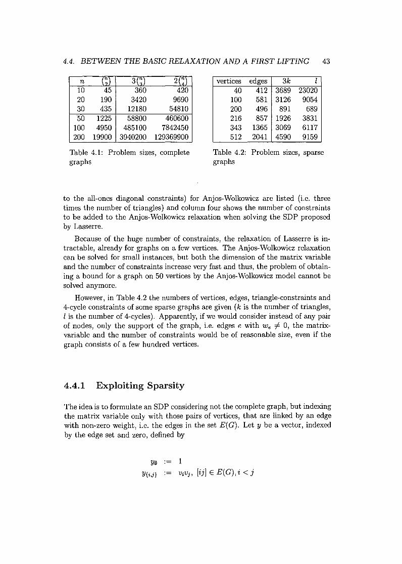
4.4. BETWEEN THE BASIC RELAXATION AND A FIRST LIFTING 43
n10203050
100200
45190435
12254950
19900
3603420
1218058800
4851003940200
2 n
4209690
54810460600
7842450129369900
vertices edges 3k l40 412 3689 23020
100 581 3126 9054200 496 891 689216 857 1926 3831343 1365 3069 6117512 2041 4590 9159
Table 4.1: Problem sizes, completegraphs
Table 4.2: Problem sizes, sparsegraphs
to the all-ones diagonal constraints) for Anjos- Wolkowicz are listed (i.e. threetimes the number of triangles) and column four shows the number of constraintsto be added to the Anjos- Wolkowicz relaxation when solving the SDP proposedby Lasserre.
Because of the huge number of constraints, the relaxation of Lasserre is in-tractable, already for graphs on a few vertices. The Anjos- Wolkowicz relaxationcan be solved for small instances, but both the dimension of the matrix variableand the number of constraints increase very fast and thus, the problem of obtain-ing a bound for a graph on 50 vertices by the Anjos- Wolkowicz model cannot besolved anymore.
However, in Table 4.2 the numbers of vertices, edges, triangle-constraints and4-cycle constraints of some sparse graphs are given (k is the number of triangles,l is the number of 4-cycles). Apparently, if we would consider instead of any pairof nodes, only the support of the graph, i.e. edges e with We =I 0, the matrix-variable and the number of constraints would be of reasonable size, even if thegraph consists of a few hundred vertices.
4.4.1 Exploiting Sparsity
The idea is to formulate an SDP considering not the complete graph, but indexingthe matrix variable only with those pairs of vertices, that are linked by an edgewith non-zero weight, i.e. the edges in the set E( G). Let y be a vector, indexedby the edge set and zero, defined by
Y0 .- 1
Y{i,j} ViVj, [ij] E E(G),i < j

44 GHAPTER 4. SDP RELAXATIONS OF THE MAX-GUT PROBLEM
Thus,1
VIV2
y= , Y E {:I::I}m+lViVj
and yyT yields the matrix:
( Y", Y0, k,l )Y = yyT =Y{i,j},0 Y{i,j},{k,l}
If this matrix corresponds to a cut, the following equalities must hold:
Y{i,k},{k,j}
Y{i,j},{k,l}
Y{i,j},{j,k}
= Y0,{i,j} 'i triangles (i, j, k) E G= Y{i,l},{j,k} 'i 4 - cycles (i, j, k, L) E G
Y{i,l},{k,l} 'i 4 - cycles (i,j,k,L) if [ik] tJ. E(G)
(4.15)
(4.16)(4.17)
Equalities (4.15) and (4.16) have already been proved in Section 4.3.1 to bevalid for matrices Y arising from a valid cut vector v. Condition (4.17) can bejustified as follows. If [ik] E E( G) then we would have the triangle-constraints:Y{i,j},{j,k} = Y0,{i,k} and Y{i,l},{k,l} = Y0,{i,k}, thus Y{i,j},{j,k} = Y{i,l},{k,l}. Sincethis edge, and therefore the constraints do not exist, we can add this conditionY{i,j},{j,k} = Y{i,l},{k,l}.
Let matrix QL E Sm+l, m = IE(G)I, be defined as
1 n-~L ..4~ 11
i=l
~Lij 'i[ij] E E(G),
where L = (Lij) is the Laplace matrix of the graph. Hence,
L: Lii Lidl Li2J2
1 Lidl 0 0QL =- Li2J2 0 04
Note, that if Y represents a cut 15(8), then
{-I
Y0,{ij} = Y{ij},0 = 1if [ij] E 15(8)otherwise.
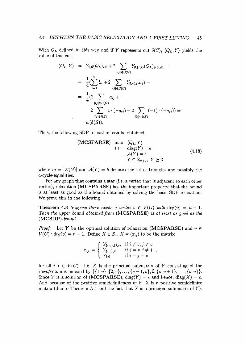
4.4. BETWEEN THE BASIC RELAXATION AND A FIRST LIFTING 45
With QL defined in this way and if Y represents cut 6(5), (QL, Y) yields thevalue of this cut:
(QL, Y) = Y0,0(Qd0,0 + 2 L Y0,{i,j}(Qd0,{i,j} =[ij]EE(G)
1 n- 4(L lii + 2 L Y0,{i,j}lij) =i=l [ij]EE(G)
1- 4(2 L aij +
(ijJEE(G)
2 L 1.(-aij)+2 L (-l).(-aij))=[ij]~8(S) [ij]E8(S)
w(6(5)).
Thus, the following SDP relaxation can be obtained:
(MCSPARSE) max (QL, Y)s.t. diag(Y) = e
A(Y) = bY E Sm+1, y!::: 0
(4.18)
where m = IE(G)I and A(Y) = b denotes the set of triangle- and possibly the4-cycle-equalities.
For any graph that contains a star (i.e. a vertex that is adjacent to each othervertex), relaxation (MCSPARSE) has the important property, that the boundis at least as good as the bound obtained by solving the basic SDP relaxation.We prove this in the following
Theorem 4.3 Suppose there exists a vertex v E V(G) with deg(v) = n - 1.Then the upper bound obtained from (MCSPARSE) is at least as good as the(MCSDP)-bound.
Proof: Let Y be the optimal solution of relaxation (MCSPARSE) and v EV(G) : deg(v) = n - 1. Define X E Sn, X = (Xij) to be the matrix
{
Y{i,v},{j,v} if i =1= v, j =1= V
Xij:= Y{i,v},0 if j = v, i =1= j ,Y0,0 if i = j = v
for all i,j E V(G). I.e. X is the principal submatrix of Y consisting of therows/ columns indexed by {{1, v}, {2, v}, ... , {v - 1, v}, 0, {v, v + I}, ... , {v, n}}.Since Y is a solution of (MCSPARSE), diag(Y) = e and hence, diag(X) = e.And because of the positive semidefiniteness of Y, X is a positive semidefinitematrix (due to Theorem A.1 and the fact that X is a principal submatrix of Y).
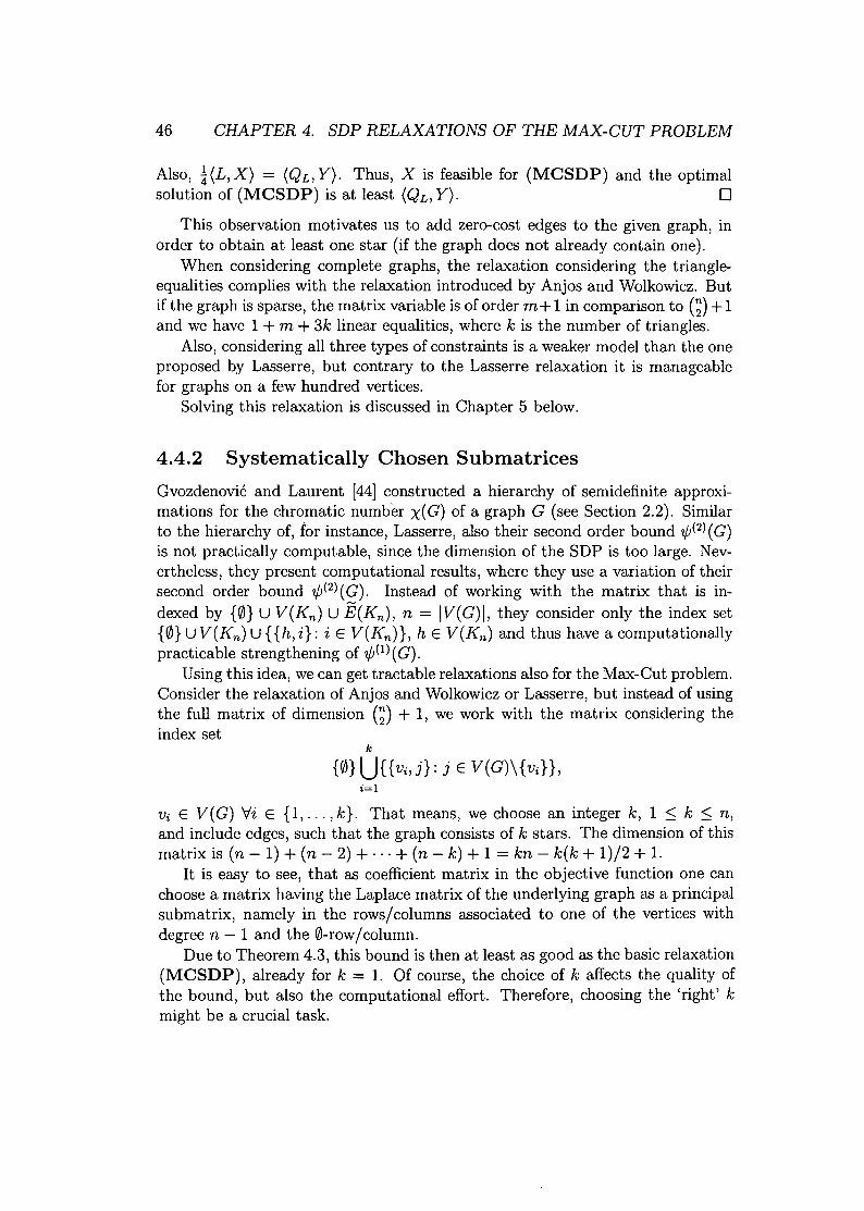
46 CHAPTER 4. SDP RELAXATIONS OF THE MAX-CUT PROBLEM
Also, ~(L, X) = (QL, Y). Thus, X is feasible for (MCSDP) and the optimalsolution of (MCSDP) is at least (QL, Y). 0
This observation motivates us to add zero-cost edges to the given graph, inorder to obtain at least one star (if the graph does not already contain one).
When considering complete graphs, the relaxation considering the triangle-equalities complies with the relaxation introduced by Anjos and Wolkowicz. Butif the graph is sparse, the matrix variable is of order m+ 1 in comparison to (;) + 1and we have 1+ m + 3k linear equalities, where k is the number of triangles.
Also, considering all three types of constraints is a weaker model than the oneproposed by Lasserre, but contrary to the Lasserre relaxation it is manageablefor graphs on a few hundred vertices.
Solving this relaxation is discussed in Chapter 5 below.
4.4.2 Systematically Chosen Submatrices
Gvozdenovié and Laurent [44] constructed a hierarchy of semidefinite approxi-mations for the chromatic number X(G) of a graph G (see Section 2.2). Similarto the hierarchy of, for instance, Lasserre, also their second order bound 'ljJ(2) (G)is not practically computable, since the dimension of the SDP is too large. Nev-ertheless, they present computational results, where they use a variation of theirsecond order bound 'ljJ(2) (G). Instead of working with the matrix that is in-dexed by {0} U V(Kn) U E(Kn), n = IV(G)I, they consider only the index set{0}UV(Kn)U{{h,i}: i E V(Kn)}, hE V(Kn) and thus have acomputationallypracticable strengthening of 'ljJ(1) (G).
Using this idea, we can get tractable relaxations also for the Max-Cut problem.Consider the relaxation of Anjos and Wolkowiczor Lasserre, but instead of usingthe full matrix of dimension (;) + 1, we work with the matrix considering theindex set
k
{0}U{{Vi,j}: jE V(G)\{và},i=l
Vi E V( G) 'Vi E {I, ... , k}. That means, we choose an integer k, 1 ::; k ::; n,and include edges, such that the graph consists of k stars. The dimension of thismatrix is (n - 1) + (n - 2) + ... + (n - k) + 1 = kn - k(k + 1)/2 + 1.
It is easy to see, that as coefficient matrix in the objective function one canchoose a matrix having the Laplace matrix of the underlying graph as a principalsubmatrix, namely in the rows/columns associated to one of the vertices withdegree n - 1 and the 0-row/ column.
Due to Theorem 4.3, this bound is then at least as good as the basic relaxation(MCSDP), already for k = 1. Of course, the choice of k affects the quality ofthe bound, but also the computational effort. Therefore, choosing the 'right' kmight be a crucial task.
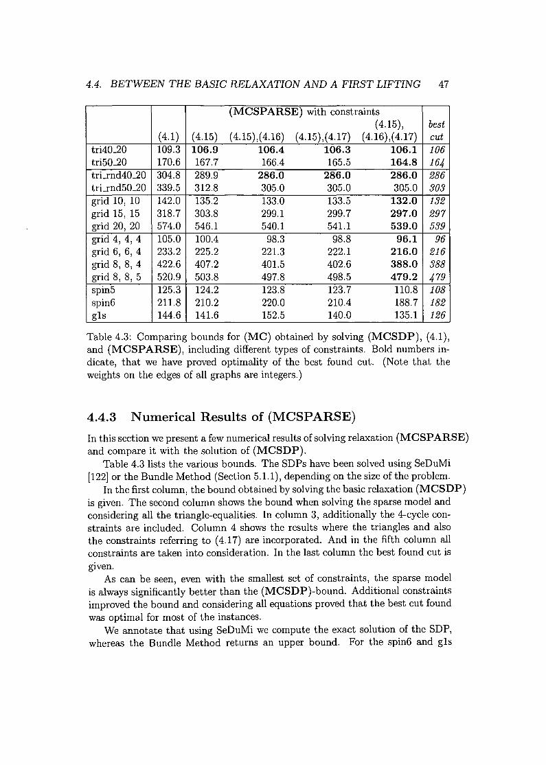
4.4. BETWEEN THE BASIC RELAXATION AND A FIRST LIFTING 47
(MCSPARSE) with constraints(4.15), best
(4.1) (4.15) (4.15),(4.16) (4.15),(4.17) (4.16),(4.17) cuttri40-20 109.3 106.9 106.4 106.3 106.1 106tri50-20 170.6 167.7 166.4 165.5 164.8 164trLrnd40_20 304.8 289.9 286.0 286.0 286.0 286trLrnd50_20 339.5 312.8 305.0 305.0 305.0 303grid 10, 10 142.0 135.2 133.0 133.5 132.0 132grid 15, 15 318.7 303.8 299.1 299.7 297.0 297grid 20,20 574.0 546.1 540.1 541.1 539.0 539grid 4,4,4 105.0 100.4 98.3 98.8 96.1 96grid 6,6,4 233.2 225.2 221.3 222.1 216.0 216grid 8,8,4 422.6 407.2 401.5 402.6 388.0 388grid 8, 8, 5 520.9 503.8 497.8 498.5 479.2 479spin5 125.3 124.2 123.8 123.7 110.8 108spin6 211.8 210.2 220.0 210.4 188.7 182gIs 144.6 141.6 152.5 140.0 135.1 126
Table 4.3: Comparing bounds for (MC) obtained by solving (MCSDP), (4.1),and (MCSPARSE), including different types of constraints. Bold numbers in-dicate, that we have proved optimality of the best found cut. (Note that theweights on the edges of all graphs are integers.)
4.4.3 Numerical Results of (MCSPARSE)In this section we present a few numerical results of solving relaxation (MCSPARSE)and compare it with the solution of (MCSDP).
Table 4.3 lists the various bounds. The SDPs have been solved using SeDuMi[122] or the Bundle Method (Section 5.1.1), depending on the size ofthe problem.
In the first column, the bound obtained by solving the basic relaxation (MCSDP)is given. The second column shows the bound when solving the sparse model andconsidering all the triangle-equalities. In column 3, additionally the 4-cycle con-straints are included. Column 4 shows the results where the triangles and alsothe constraints referring to (4.17) are incorporated. And in the fifth column allconstraints are taken into consideration. In the last column the best found cut isgiven.
As can be seen, even with the smallest set of constraints, the sparse modelis always significantly better than the (MCSDP)-bound. Additional constraintsimproved the bound and considering all equations proved that the best cut foundwas optimal for most of the instances.
We annotate that using SeDuMi we compute the exact solution of the SDP,whereas the Bundle Method returns an upper bound. For the spin6 and gIs

48 CHAPTER 4. SDP RELAXATIONS OF THE MAX-CUT PROBLEM
graphs, the relaxation with constraints (4.15),(4.16) (which is intractable to besolved by SeDuMi) was hard to solve for the Bundle Method. The progress wasnot satisfactory and therefore we end up with a bound that is rather far from theoptimum of the SDP. Nevertheless, the Bundle Method for solving the relaxationusing constraints (4.15),(4.16),(4.17) shows a more satisfying behavior and thebounds for graphs spin6 and gIs are improved significantly.
Chapter 5
Algorithms for SolvingLarge-Scale SemidefinitePrograms
In previous chapters we investigated various Semidefinite Programs for solving orapproximating NP-hard problems arising from Combinatorial Optimization. Thischapter is dedicated to methods for solving these SDPs. Two prominent solutionmethods have already been investigated in Chapter 1, namely the Interior-PointMethod and the Spectral Bundle Method. Although these two methods arewidely used, for various kinds of relaxations the dimension of the matrix variableor the number of constraints is simply too large to be solved by one of thesealgorithms.
This means that for various NP-hard problems promising Semidefinite Pro-gramming relaxations exist, but due to the vast computational effort or the hugememory requirements, the SDPs are not solvable.
Another way to tackle the problems of solving these SDPs, is using Lagrangianduality and then solving the underlying problem by Bundle Methods, a tool foroptimizing non-differentiable functions (see Schramm and Zowe [118], Kiwiel [70],Lemarechal [82]). We will focus on these methods in this chapter and will elab-orate the details for solving the relaxations introduced in the previous chapter.Furthermore, we will come back to the Spectral Bundle Method, introduced inSection 1.4.2 and establish second order models to improve the performance.Finally, the Boundary Point Method is introduced in this chapter. This newalgorithm uses an augmented Lagrangian algorithm applied to the dual SDP. Atthe end of the chapter, a brief guidance for choosing the proper algorithm to solvea given SDP is presented.
49
50 CHAPTER 5. ALGORITHMS FOR SOLVING LARGE-SCALE SDPS
5.1 The Bundle Method in Combinatorial Op-timization
Barahona and Anbil [11]and Barahona and Ladanyi [12]use the volume algorithmfor solving LP relaxations arising from combinatorial optimization problems. Thisalgorithm allows solving LPs with a large number of constraints, because theyare not handled directly, but are incorporated by using the Lagrangian dual.Bahiense, Maculan, and Sagastizabal [7])show that this algorithm can be viewedas a simple variant of the Bundle Method.
Bundle Methods were first proposed by Lemarechal [82], and later on furtherinvestigated by Kiwiel [69],Lemaréchal, Nemirovskii, and Nesterov [83]. A recentsurvey can be found in the paper of Mäkelä [91]. A detailed presentation can befound in the textbook of Hiriart-Urruty and Lemaréchal [60].
We want to apply this method to solve semidefinite programs with a largenumber of constraints, for example those introduced in Sections 4.2 and 4.4.
The ingredients of the Bundle Method are basically the following:
• For a convex objective function 1 and a point 1E lRm we are able tocompute
- the objective value 1(1)- a subgradient 9 E ô1(i), i.e. 9 satisfying
• This information is used to construct a cutting plane model j of I, mi-norizing 1 on lRm
:
• Since the quality of minorant j is reasonable only in the vicinity of thecurrent iterate, displacement is penalized by considering
where u E lR is the penalty parameter.
The bundle (of size k) can be seen as the set of triples
We sketch the generic framework as follows.

(5.1)
5.1. THE BUNDLE METHOD IN COMBINATORIAL OPTIMIZATION 51
Algorithm 5.1 (Generic Bundle Algorithm)Input.
Function fand 1E IRm.Start.
Evaluate f (1) and obtain subgradient g.Construct cutting plane model Î of f, minorizing f on IRm.
while some stopping condition is not satisfiedSolve min-yÎh) + ~II, - 1112to get 'test.Evaluate f at ,test and obtain subgradient gtest.if reasonable progress is made
Do a serious step,update bundle, giving updated l
elseDo a null step,update bundle, giving updated l
Check stopping condition.end
In the two subsequent sections we want to elaborate the details for applying theBundle Method to solve SDP relaxations of the Max-Cut problem.
5.1.1 Solving (MCSPARSE) Using the Bundle Method
We want to solve the Max-Cut relaxation introduced in Section 4.4, namely
(MCSPARSE) max (QL, Y)s.t. diag(Y) = e
A(Y) = bY E Sm+l, Y t: 0
where m = IE(G)I and A(Y) = b denotes the set of triangle- and possibly the4-cycle-equalities. Let l be the number of these constraints, Le. b E IRl.
Recall that the set of positive semidefinite matrices with an all-ones diagonalis the elliptope, denoted by £. Thus, (5.1) can equivalently be written as
(MCSPARSE) max (QL, Y)s.t. A(Y) = b
Y E£.(5.2)
The goal is to optimize the dual functional to (MCSPARSE). Let us introducethe Lagrangian
£(Y, ,) := (QL, Y) + ,T(b - A(Y»
and the dual functional
(5.3)
52 CHAPTER 5. ALGORITHMS FOR SOLVING LARGErSCALE SDPS
Evaluating f for some 'Yamounts to solving a problem of type (4.1), which canbe done easily for problem sizes of our interest by Interior-Point Methods (seeSection 1.4.1).
We call apair ("{,Y) a matching pair for f, if f("{) = £(Y, 'Y). A subgradientis given by g("{) = b-A(Y). By applying Corollary A.12 we obtain the Lagrangiandual
maxmin£(Y,'Y) = minmax£(Y,'Y) = minf("{).YE£ ~. ~ YE£ ~
Following the ideas of the bundle concept, we build up a bundle of matricesto construct the minorant
fappr("{) := max{£(Y, 'Y): Y E conv(Y1, ... , Yk)}.
Obviously, Y E conv(Y1, ... , Yk) can be expressed as Y = >'1Y1+ ... + ÀkYk,eTÀ = l,À ~ O.
In each iteration we have some current iterate1' and we have to solve
(5.5)
which is convex quadratic in 'Y, and then we find Y (i.e. solving an SDP ofdimension n with n linear constraints), such that ("{,Y) is a matching pair.
Some notation. Let us collect Yi, ... ,Yk symbolically in y and for a vectorÀ E IRk define YÀ := L:7=1 ÀiYi. Furthermore we define A := {À E IRk: eTÀ =1, À ~ a}. G E IR1xk is the collection of the k subgradients, i.e. G := (gl, ... , gk)and F E IRk is the vector of the primal function values of the matrices in y, Le.Fi:= (QL,Yi), 1~ i ~k.
With this notation we rewrite
f appr ("{ ) max bT'Y+ (QL - AT ("{), Y À) =ÀEAmax (b - A(YÀ), 'Y)+ (QL, YÀ) =ÀEAmax'YTGÀ + FTÀ.ÀEA
Therefore, (5.5), the problem to be solved, reads
min max 'YTGÀ + FT À + 21iI'Y - 1'112=~ ÀEA t
= max min 'YT GÀ + FTÀ + 2
1tiI'Y - l'11
2.ÀEA ~
(5.6)
The inner problem in (5.6) is an unconstrained convex quadratic problem in 'Yand therefore we can replace the minimization by insuring t~(.)= 0:
GÀ + !("{ - 1') = at'Y = l' - tGÀ. (5.7)
5.1. THE BUNDLE METHOD IN COMBINATORIAL OPTIMIZATION 53
Substituting (5.7) in (5.6) we obtain
max,T GÀ + pT À + 2-1IT - 1'112=ÀEA 2t
- max(1' - tGÀ)TGÀ + pTÀ + ~II1' - tGÀ - 1'112=ÀEA 2t
- max1'TGÀ - tllGÀI12 + pTÀ + -2tIIGÀII2 =
ÀEA
- max(GT1' + pfÀ - -2tIIGÀII2. (5.8)
ÀEA
This convex quadratic problem over A can be solved efficiently by an Interior-Point Method.
We can summarize now the algorithm to solve problem (5.1).
Algorithm 5.2 (Bundle Method to solve (MCSPARSE))Input.
QL, A, b defining the problem.Starting point l' E ]Rm (optional).Parameter t, a, é.
Start.i=l, done=lalse.Evaluate 1 at 1':
solve max (QL - AT(1'), Y) s.t. Y E £ giving Y,1 (1') = bTl'+ (QL - AT (1'), Y) ,subgradient G = g(1') = b - A(Y).
repeatSolve (5.8) and obtain À.
,test = l' - tGÀ.lappr(,test) = (P + GT,test)TÀ.ifi < itermax and 1(1') - lappr(,test) > é
Evaluate 1 at ,test:solve max (QL - AT(,), Y) s.t. Y E £ giving Y'test,Itest = bT,test + (QL - AT(,test), Y'test),subgradient gtest = b - A(Y'test).
if Itest ::; alappr(,test) + (1 - a)I(1')Serious step:l' = ,test.Increase t.
elseNull step:Decrease t.
Purge bundle (*).Append Y'test to y, gtest to G, (QL, Y'test) to P.

54 CHAPTER 5. ALGORITHMS FOR SOLVING LARGFrSCALE SDPS
i=i+l.else
done=true.until done.
ad (*): In order to keep the size of the bundle reasonably small, we purge it ineach iteration, meaning that we eliminate points Yi from y (and corresponding Fiand the i-th column of G) whose contribution to the minorant Jappr is negligiblysmall (i.e. 'xi < p' maxl:Sj:Sk'xj, for small P > 0).
Computational effort. Solving problem (5.8) can be done efficiently and alsothe matrix and vector manipulations are of minor computational effort. Themost expensive task during one iteration is the function evaluation, i.e. solvingan SDP of dimension m with the m equality constraints fixing the main diagonalto all ones. This SDP has to be solved exactly once in each iteration. Therefore,one has to limit the number of iterations in order to get reasonable computationtimes.
Quality of the solution obtained by the Bundle Method. Since the Bun-dle Method returns only a "nearly" optimal solution, we want to evaluate thequality of this solution. We run the following experiment. Instances, which aresolvable by Interior-Point Methods, as well as by the Bundle Method, are cho-sen and solved using SeDuMi (Sturm [122]) and using our Bundle code, fixingthe number of iterations to 100. (In detail, we set the parameters as follows:c = lQ-8, a = 0.2, estimate for t: t = 2(f(-Ystart) - best)j(GTG), where best issome best known lower bound; if serious step: t = 1.0It, if null step: t = tj1.02.)We summarize the results in Table 5.1. It turns out, that the bundle solution isalways less than 1% above the solution of the Interior-Point Method and thereforeit is definitely arguable to talk about a "nearly" optimal solution.
5.1.2 Solving (SDPMET) Using the Bundle Method
Fischer, Gruber, Rendl, and Sotirov [35] developed a dynamic version of theBundle Method to solve problem
(SDPMET) max (L, X)s.t. A(X)::; b
XE£,(5.9)
where A(X) ::; b denotes the set of triangle inequalities (see Section 4.2).Contrary to solving (MCSPARSE), explained in Section 5.1.1, we have to
deal with inequalities, instead of equalities, which requires further examination.
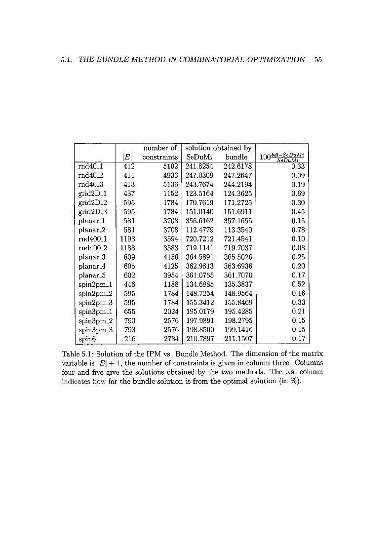
5.1. THE BUNDLE METHOD IN COMBINATORIAL OPTIMIZATION 55
number of solution obtained bylEI constraints SeDuMi bundle 100bdl-SeDu~i
rnd40_1 412 5102 241.8254 242.6178 0.33rnd40_2 411 4933 247.0309 247.2647 0.09rnd40_3 413 5136 243.7674 244.2194 0.19grid2D_1 437 1152 123.5164 124.3625 0.69grid2D_2 595 1784 170.7619 171.2725 0.30grid2D_3 595 1784 151.0140 151.6911 0.45planar_1 581 3708 356.6162 357.1655 0.15planar_2 581 3708 112.4779 113.3540 0.78rnd400_1 1193 3594 720.7212 721.4541 0.10rnd400_2 1188 3583 719.1141 719.7037 0.08planar_3 609 4156 364.5891 365.5026 0.25planarA 605 4125 362.9813 363.6936 0.20pianaL5 602 3954 361.0765 361.7070 0.17spin2pm_1 446 1188 134.6885 135.3837 0.52spin2pm_2 595 1784 148.7254 148.9564 0.16spin2pm_3 595 1784 155.3412 155.8469 0.33spin3pm_1 655 2024 195.0179 195.4285 0.21spin3pm_2 793 2576 197.9891 198.2795 0.15spin3pm_3 793 2576 198.8500 199.1416 0.15spin6 216 2784 210.7897 211.1507 0.17
Table 5.1: Solution ofthe IPM vs. Bundle Method. The dimension oft he matrixvariable is lEI + 1, the number of constraints is given in column three. Columnsfour and five give the solutions obtained by the two methods. The last columnindicates how far the bundle-solution is from the optimal solution (in %).
56 CHAPTER 5. ALGORITHMS FOR SOLVING LARGE-SCALE SDPS
We now have to solve the Lagrangian dual
min f(r),'Y~O
with f defined in (5.4). Dualizing also the constraints "( 2:: 0, we obtain
max min "(TG>' + pT>. + ~II"( - 1112 - "(T'flÀEA,7J~O 'Y 2t
(5.10)
where in addition to (5.6) we have 'fl, the Lagrange multipliers to the constraints"( 2:: O. As before, the inner minimization can be replaced by setting the derivativewith respect to "( to zero yielding
"(=1- t('fl - G>').
Plugging this into (5.10) we obtain
(5.11)
(5.12)
This is a convex quadratic optimization problem in >.and 'fl. Solving it directlyis too time consuming and thus, we solve it approximately by alternately keepingone set of variables constant. Keeping 'fl constant leads to a convex quadraticproblem similar to (5.8). Keeping>. fixed (say, >'), we obtain
The maximizer fi to this problem can be determined coordinate-wise:
(see for instance Helmberg, Kiwiei, and Rendl [57]). This process of keepingone set of variables constant is iterated several times, and we end up with anapproximate solution of (5.12).
A further difference to the algorithm described in Section 5.1.1 is, that thefunction f(r) to be minimized is not considered to be fixed, but changes in thecourse of the algorithm. This is due to the fact, that we do not want to considerall the triangle-inequalities at the same time, since the number of them is of orderO(n3
) (n is the dimension of X).As initial function we solve
max{ (L,X): XE £}
5.1. THE BUNDLE METHOD IN COMBINATORIAL OPTIMIZATION 57
yielding an initial maximizer X*. We could now define Jb) by dualizing all theconstraints A(X) ::; b, but to maintain efficiency,we are interested only in thoseconstraints, which are likely to be active at the optimum. Therefore we look atthe violation r* := b-A(X*) and set rmin:= min{r;}. In the unlikely event thatrmin~ 0, X* is optimal for (SDPMET) and we are done. Otherwise rmin < 0and we consider now only those constraints from A(X) ::; b which are 'badly'violated by X* to define J.
Specifically, let 0 < Π< 1 and set
We denote by AI the operator that contains only those matrices Aï, which cor-respond to the triangle-inequalities in I. Similarly, we define bIo For notationalconvenience we denote
Thus we start by minimizing fI using the Bundle Method described above. Af-ter a preassigned number of bundle iterations, some 'YI and some X are obtained.It is likely that 'YI is still far from the true minimizer of fI. Before continuingwith further iterations, we will update I, the index set ofthe triangle-inequalitiesunder consideration, by removing those which seem to be not important andadding those, that promise progress. Thus, we need to answer the following twoquestions:
• Which of the constraints in J should be kept?
• Are there additional constraints that should be added to I?
To answer the first question, we use 'YI' A large value 'Yi indicates that theconstraint i is binding and hence should not be removed. 'Yi = 0 indicates thatconstraint i may be inactive, and therefore could be removed. In summary, we use'YI to purge J by removing constraints i with a value 'Yi smaller than a prescribedfraction of max( 'YI).
It is less obvious to decide which new constraints should be added to J. Ex-periments showed that using a convex combination of X and the previous pointXo1d to identify violated constraints gives the most satisfactory behaviour of thealgorithm.
Numerical results for using this method to solve (SDPMET) can be foundin [35, Table 4]. The algorithm reduces the gap of the basic SDP relaxation (4.1)by 20% up to 90% for medium sized graphs (n ::; 512), and by at least 10% forlarger graphs (729 ::; n ::;2000). No other method so far is capable of producingsimilar or even better bounds.
58 CHAPTER 5. ALGORITHMS FOR SOLVING LARGE-SCALE SDPS
5.2 The Spectral Bundle Method with SecondOrder Information
What follows in this section is based on joint work with Armbruster, Overtonand Rendl [4]. We will use within this section definitions and formulas fromSection 1.3 (Eigenvalue Optimization) and Section 1.4.2 (The Spectral BundleMethod).
Although the Spectral Bundle Method is capable of solving quite large-scaledSemidefinite Programs, convergence is very slow. Within the method, the regu-larized model (1.17)
min{Î(y) + ~IIY _yI12}yElRk 2
is optimized. Since the choice of the parameter u is "somewhat of an art" (seeRemark 1.14), the idea is to replace uI by making partial use of second orderinformation and thus solve the following problem:
~ 1 ~min{f(y) + -2(y -yfH(y -y)},yElRk
where ÎI is a suitable approximation of the Hessian matrix of l With this choicewe hope to get a better performance of the algorithm.
To work out the details, what a "suitable approximation" of the Hessian is,recall definition (1.16)
Here we define
Î(y) := max (C - AT(y), W) + bTy.WEW
(5.13)
w:= {PVpT: trV = 1,V ES:},
with integer k being significantly smaller than n. Thus (1.18), the problem to besolved in the course of the algorithm, becomes
and (1.19) readsy = y + ~(A(PV pT) - b).
u(5.15)
In order to derive a second order model, let us explore the derivatives of thefunction in question. Let
be the spectral decomposition, where Q = (ql, q2, ... , qn) is an n x n matrix,QTQ = I, À1 > À2 ~ ... ~ Àn, A = Diag(Àl" .. ,Àn).
(5.16)
(5.17)
5.2. SPECTRAL BUNDLE WITH 2ND ORDER INFORMATION 59
Assuming that the largest eigenvalue is simple, function Àmax(C- AT(y)) issmooth and we obtain
8 ( T( T~Àmax C - A y)) = -ql Aql,UYi
82T ) -1 T8 8 Àmax(C - A (y) = 2qlAiQ2(ÀIln-I - D2) Q2 Ajql,
Yi yj
where Q2 = (q2, ... , qn), D2 = Diag(À2, ... ,Àn), see for instance Lancaster [75].In general, the largest eigenvalue will have multiplicity k > 1. In this case,Àmax(C- AT(y)) may not be written as a differentiable function in general.
Overton and Womersley [101] develop a second order model to minimize func-tion Àmax(A(x)) with A(x) being a sufficiently smooth symmetric matrix. Ourapproach is closely related to this even more general work.
Suppose the largest eigenvalue Àmax(C- AT(y)) has multiplicity k, i.e.
and partition Q in QI and Q2, such that
For finding a suitable approximation of the Hessian, we first need a matrix W =PV pT. Recall from (1.10) that condition A(PV PT) = bmust hold for optimality.Now QI plays the role of P in Section 1.3, and to avoid confusion let us use Uinstead of V. Therefore, one way to find a proper U is to solve the problem
mm lib - A(Q1UQf)112s.t. trU = 1
UtO(5.18)
and then define W := Q1UQf. In this way we obtain a subgradient g(y) =b - A(W) E 8f(y) of minimum norm. If A(W) = b, then 0 E 8f(y) holds andhence, we have a certificate for optimality.
We use matrix U to define the following matrix H(U) = (hij),
hij = 2tr(A(QIUQf)AjQ2(ÀIln-k - D2)-lQf)
with D2 = Diag(Àk+l"'" Àn). Matrix H(U) captures the second order behaviourof f(y) around the current point y with k being the multiplicity of the largesteigenvalue of C-AT(y), see Helmberg and Oustry [53]or Overton and Womersley[101]. In the case of a simple largest eigenvalue, H(U) indeed coincides with theHessian of f(y).
By using H(U) instead of uI in (5.15) we get
y = y + H(U)-l(A(W) - b). (5.19)
60 CHAPTER 5. ALGORITHMS FOR SOLVING LARGE-SCALE SDPS
Plugging this and H(U) into (5.14), the program to be solved, we obtain
maxW=QIVQ[ (C - AT(Y), W) + bTy - ~(y - yl H(U)(y - y) =trV=l,V1::0
= maxW=QIVQ[ (C - AT(Y + H(U)-I(A(W) - b)), W) +trV=l,V1::0
+bT(Y + H(Utl(A(W) - b)) +
+~(-H(U)-I(A(W) - b))TH(U)(-H(U)-I(A(W) - b)) =
= maxW=QIVQ[ (C - AT(y) + AT(H(U)-lb), W) +trV=l,V1::0
_~(AT(H(U)-IA(W)), W) + bTy - ~bTH(U)-lb.
By defining
AT(H(U)-IA(W))C - AT(y) + AT(H(U)-lb)
C3 '- bTy - ~bTH(U)-lb2
we end up with the quadratic problem
max{ -(CI(W), W) + (C2, W) + C3: W = QI VQf, trY = 1, V tO}. (5.20)
We can now outline the algorithm as follows.
Algorithm 5.3 (Spectral Bundle Method with Second Order Information)Input.
C, A, b defining the problem.Starting point y E ~m (optional).Parameter iter max and €.
Start.Evaluate f at y:
Compute spectral decomposition C - AT(y) = QAQT,f(y) = -Xl + bTy.
Estimate k, the multiplicity of -Xmax.
QI = (ql, ... , qk)repeat
Solve (5.18) and obtain U.Compute H(U).Solve (5.20) and obtain W.Compute direction d = H(U)-I(A(W) - b) (see (5.19)).Do a line search and obtain t in y = y + td.y f- Y + td.
5.2. SPECTRAL BUNDLE WITH 2ND ORDERINFORMATION 61
Evaluate f at the new point y and obtain new Q.Estimate k, the multiplicity of Àmax.
QI = (Q11 ... ,Qk).until iter max reached or IIdll < é.
Four items of this algorithm need further comments:
• Eigenvalue computation .
• Variation of H(U) in order to gain computational efficiency.
• Guessing the multiplicity of Àmax.
• Line search.
Eigenvalue computation. The eigenvalue computation can be done efficientlyby iterative methods, see Parlett [104]. There exist several implementations ofthese methods, for instance, the Arnoldi method [5]can be found in the ARPACKpackage [81].
Variation of H(U). Computing matrix H(U) and the inverse ofit requires sub-stantial computational effort. A way to replace these operations by much cheaperones, is to use only the main diagonal of H(U) and ignore the off-diagonal en-tries. In this way we still utilize second order information, but require only cheapmatrix operations and have therefore a computationally practical algorithm.
Multiplicity of Àmax. The multiplicity of the largest eigenvalue is usually notknown in advance and therefore we have to cleverly guess this value. We computethe differences of the normalized eigenvalues
~À' '= _À_i-_À_i+_1 1< . < - 1t • À
1' - 'I, _ n .
If ~À1 is a value larger than, say 0.01, we can assume the eigenvalue À1 to besimple. Otherwise, the multiplicity is k, if there is either a relatively to ~À1 largegap ~Àk, or if the difference between À1 and Àk is considerably big, i.e.
with [) being for instance 0.05.
62 CHAPTER 5. ALGORITHMS FOR SOLVING LARGE-SCALE SDPS
Line search. Lancaster [75] shows that for any matrix C(t) whose elementsare functions of a scalar parameter t, the function À(C(t)) has continuous secondderivatives with respect to t. We can use this in the line search, by computingthe Taylor expansion up to order two of f(Y + td) and therefore, have a cheapway of computing the approximate function value. I.e. if we know 'xmax(t) and).max(t), we can compute
f(Y + td) - Àmax(C - AT(y + td)) + bT(y + td) =- Àmax((C - AT(Y)) + tAT(d)) + bTy + t(bT d) ~
T ~ T~' T t2 ..~ Àmax(C - A (y)) + b y + t((Àmax(t)) + b d) + 2Àmax(t).
Note, that eigenvalue Àmax(C - AT(Y)) is already known in the current iteration.To work out the details what 'xmax(t) and ).max(t) is, consider
with C and D being symmetric n x n matrices, and Ài denotes the i-th eigenvalueof the matrix in question. We also assume that eigenvalues are sorted in non-increasing order, i.e. À1 ~ ... ~ Àn. (Applied to our function, C corresponds toC - AT(Y) and D to AT(d).)
We rewrite the relevant theorems, applied to our problem. Note, that thetheorems concerning existence of the eigenvalues (following from the theory ofimplicit functions and the work of Goursat [40]) and differentiability can also befound in the paper of Lancaster [75].
Theorem 5.4 Lancaster [75, Theorem g}Assume that all eigenvalues Ài' 1 ::; i ::;n, of B(to) = C + toD, with spectraldecomposition B(to) = XAXT, XTX = XXT = I, are distinct. Then for aneigenvalue Ài of B(to) we have
where
'xi(tO) = Pii,n 2
).i (to) = 2L À. ~ À. 'j=l t JNi
p = XTDX.
(5.21)
(5.22)
(5.23)
Proof: First, by differentiating XT X = I we get j(T X + XT j( = 0 and definethe skew-symmetric matrix
'T T .S:=X X=-X X. (5.24)

5.2. SPECTRAL BUNDLE WITH 2ND ORDERINFORMATION 63
Now, we differentiate A = XT EX and by defining P = XT DX and (5.24) weobtain
A(to) - XTEX+XTDX+XTEX=XTDX +XTXXTEX +XTEXXTX =
- P+SA-AS.
For the diagonal elements we obtain
The off-diagonal elements have to be zero and thus,
)..ij(tO) = 0 ~ Pij + Sij).,j - ).,iSij = 0Pij
~ Sij = ).,i _ ).,j for i =I- j.
And since S is skew-symmetric we have
Sii = O.
To compute .Ài(to) we differentiate P.
P = XTDX+XTDX=_ XTXXTDX+XTDXXTX=
(XTX)(XTDX) - (XTDX)(XTX) =- SP-PS.
And since P is symmetric and S skew-symmetric, we obtain
n n n
Pii = L SijPji - LPijSji = 2 L Sijpji'j=l j=l j=l
Combining this with (5.26) and (5.27), we finally get
n 2.. . ~ Pij).,i ( to) = Pii = 2 ~ ).,. _ ).,..
;=1 t J#i
(5.25)
(5.26)
(5.27)
oFormula (5.22) will not hold in the presence of multiple eigenvalues. In this
case the following theorem applies.
64 CHAPTER 5. ALGORITHMS FOR SOLVING LARGE-SCALE SDPS
Theorem 5.5 Lancaster [75, Theorem 10]Assume that the largest eigenvalue >-lof B(to) = C + toD has multiplicity k,i.e. >-I = ... = >-k > >-k+l 2: ... 2: >-n. The spectral decomposition of B(to) isgiven by B(to) = XAXT, XTX = XXT = I, with X = [Xk Xn-k], Xk E jRnxk,Xn-k E jRnx(n-k). Furthermore, Xl DXk has eigenvalues 'l/Jl,' .. , 'l/Jkand denotethe spectral decomposition of this product by Y'lJyT, with W = Diag( 'l/Jl, ... ,'l/Jk)'Then for 1~ i ~k it follows
).i(tO) = Pii,n -2
'\i(to) = 2 L >-.~ >-. 'j=k+l t J
where
Using these two theorems, we can do several function evaluations during theline search, without explicitly computing the largest eigenvalue.
5.3 A Boundary Point MethodThe work presented in this section has been done jointly with Povh and Rendl[110].
A further method for solving Semidefinite Programs apart from the one pre-sented so far, has been proposed by Burer and Vandenbussche [27]. Theyapplythe Augmented Lagrangian technique to the primal SDP. Malick [92]uses a sim-ilar approach for solving semidefinite least squares problems.
We will take up the idea of using the Augmented Lagrangian technique, butwill contrary to [27] apply it to the dual SDP, which is given as
(DSDP) mm (b, y)S.t. AT(y) - C = Z
Y E jRm, Z E Sn, Z t: O.
Throughout this section, we make the assumption that the Slater condition (Def-inition 1.6) is satisfied.
We introduce a Lagrange multiplier X and consider for fixed {J > a the aug-mented Lagrangian
5.3. A BOUNDARY POINT METHOD 65
(5.28)
that has to be minimized. The Augmented Lagrangian method applied to ourproblem can be sketched as follows (see Bertsekas [22]).
Algorithm 5.6 (Augmented Lagrangian method to solve (DSDP»Input.
C,A,b.Initialization.
k = O.Select O"k> 0, Xk t O.
while some stopping condition is not satisfiedKeep Xk fixed andsolve miny,zto LUk (y, Z; X) giving Yk, Zk.Update X: Xk+1 = Xk + O"(Zk + C - AT(Yk».Select O"k+l2: O"k.Check the stopping condition and increase k.
return (Xk, Yk, Zk).
To simplify notation, we define
W(y) := AT(y) - C - .!X,0"
and rewrite the augmented Lagrangian as0" 1
Lu(Y,Z;X):= bTy+ "2IIZ - W(Y)112 - 20"11X1I2.
Thus, the minimization in Algorithm 5.6 reads
min bTy + ~IIZ - W(y)112.y,ZtO 2(5.29)
This is a convex quadratic SDP and therefore tractable. However, when lookingat the optimality conditions of this SDP, one can find a cheap way of solving itby iteratively keeping one set of variables fixed.
To derive the optimality conditions of this problem, let us introduce the La-grange multiplier V for the constraint Z t 0:
L(y, Z; V) = bTy + ~IIZ - W(y)1I2 - (V, Z).
Computing the derivatives of L(y, Z; V) with respect to y and Z, we get:1
"VyL(Y, Z; V) = b - O"A(Z - AT(y) + C + -X) =0"
1= O"A(AT(y» - O"A(Z + C + -X) + b,
0"1
"VZL(y, Z; V) = O"(Z - AT(y) + C + -X) - V =0"
O"(Z - W(y» - V,
66 CHAPTER 5. ALGORITHMS FOR SOLVING LARGE-SCALE SDPS
and by setting these derivatives equal to zero, we obtain the following KKTconditions, necessary for optimality:
1\ly£(Y, Z; V) = 0 => o-A(AT(y)) = aA(Z + C + -X) - b,
a\l z£(y, Z; V) = 0 => V = a(Z - W(y)), (5.30)
V t 0, Z t 0, V Z = o.Since the problem is convex and the Slater condition holds, these conditions arealso sufficient for optimality.
We observe that keeping y (and X) constant, Z is given by the projection ontothe cone of positive semidefinite matrices and thus, Z must satisfy the projectioncondition
(5.31)
It is well known, that W(y)+ can be computed via the eigenvalue decompositionof W(y), see for instance Higham [58]. This works as follows. Let W(y) = P ApT,pT P = I, A = Diag(,\), and partition P and A according to its non-negativeand negative eigenvalues: A = Diag(A+, A_), P = (P+ P_) with Al ~ 0, A2 < o.Therefore,
W(y) = P+A+PJ. + P_A_P!. = W(y)+ + W(y)_.
On the other hand, keeping Z (and X) constant, the minimization prob-lem (5.29) is unconstrained and y can be computed by solving the linear system
1aA(AT(y)) = aA(Z + C + -X) - b.
a(5.32)
Furthermore, from (5.30) we get V = a(Z - W(y)) = a(W(y)+ - W(y)) =-aW(y)_. Thus, we can reformulate conditions (5.30) as
1 1A(AT(y)) = A(Z + C + -X) - -b,
a aZ = W(y)+,
V = -aW(y)_.
Keeping one set of the variables (y or Z) constant leads to problems that areeasy to solve. Thus, we carry out minimization (5.29) by iteratively alternatingbetween solving (5.32) and computing Z by projection (5.31).
The minimization is then followed by the update on X (see Algorithm 5.6),which can with (5.28) and (5.31) be simplified to
Xnew - X+a(Z+C-AT(y))=
= -a(W(y) - W(y)+) =- -aW(y)_.
5.3. A BOUNDARY POINT METHOD 67
The Lagrange multiplier V is therefore indeed identical with the primal matrixX.
Note, that throughout the algorithm, the conditions X ~ 0, Z ~ 0 andZX = 0 hold. Therefore, we call this algorithm a boundary point method, asboth, Z and X, are on the boundary of the cone of semidefinite matrices. Oncewe have reached feasibility regarding the primal and dual linear equations, wehave an optimal solution. Thus, primal and dual feasibility will serve as thestopping criterion in the algorithm.
Summarizing, we can now state the Boundary Point Method as the following
Algorithm 5.7 (Boundary Point Method)Input.
C,A,b.Initialization.
k = O.Select a> 0, E > 0, {Ed ~ o.Xk = 0, Zk = o.
repeatrepeat
solve A(AT(y)) = A(Zk + C + lXk) - lb giving Yk.T 1 a aW(Yk) = A (Yk) - C - -;;Xk.
Zk = W(Yk)+.Vk = -aW(Yk)_.Dinner = iIA(Vk) - bll.
until Dinner:::; aEk.
Xk+l = Vk.
Douter = IIZk - AT(Yk) + Cil.k=k+1.
until Douter :::;E.
The highest computational costs arise in computing the spectral decompositionof matrix W(y) and in solving the system of linear equations (5.32). Contraryto Interior-Point Methods where the system matrix changes in each iteration, inthe Boundary Point Method the matrix arising from A(AT(.)) remains the samethroughout the algorithm. By computing for instance the QR-decompositiononly once, at the beginning of the iterations, one can obtain Yk by performingbacksolves. Moreover, for some problems the system-matrix of (5.32) is simplya diagonal matrix and therefore the computation times for solving the equationsare negligibly small.
For the theoretical convergence results the reader is referred to Povh et al.[110]. Therein numerical results of computing the 'l9-number of a graph are alsogiven. These results show that the Boundary Point Method works very well onthese instances. Comparison to the most efficient codes currently available, which
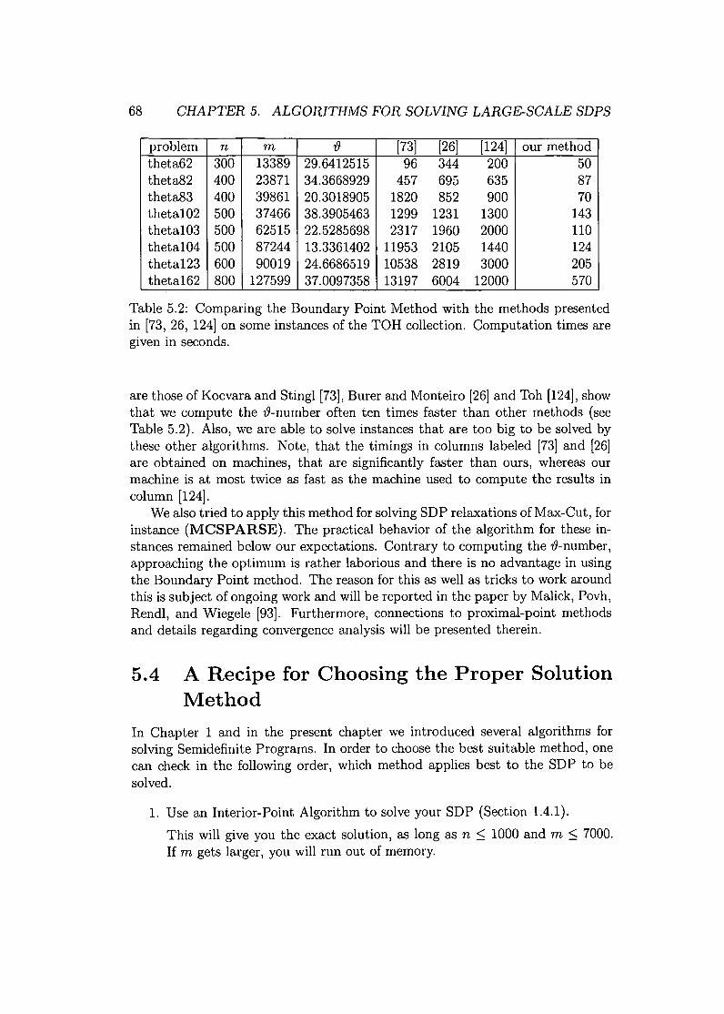
68 CHAPTER 5. ALGORITHMS FOR SOLVING LARGE-SCALE SDPS
problem n m rJ [73] [26] [124] our methodtheta62 300 13389 29.6412515 96 344 200 50theta82 400 23871 34.3668929 457 695 635 87theta83 400 39861 20.3018905 1820 852 900 70theta102 500 37466 38.3905463 1299 1231 1300 143theta103 500 62515 22.5285698 2317 1960 2000 110theta104 500 87244 13.3361402 11953 2105 1440 124theta123 600 90019 24.6686519 10538 2819 3000 205theta162 800 127599 37.0097358 13197 6004 12000 570
Table 5.2: Comparing the Boundary Point Method with the methods presentedin [73, 26, 124] on some instances of the TOR collection. Computation times aregiven in seconds.
are those of Kocvara and Stingl [73], Burer and Monteiro [26] and Toh [124], showthat we compute the rJ-number often ten times faster than other methods (seeTable 5.2). Also, we are able to solve instances that are too big to be solved bythese other algorithms. Note, that the timings in columns labeled [73] and [26]are obtained on machines, that are significantly faster than ours, whereas ourmachine is at most twice as fast as the machine used to compute the results incolumn [124].
We also tried to apply this method for solving SDP relaxations of Max-Cut, forinstance (MCSPARSE). The practical behavior of the algorithm for these in-stances remained below our expectations. Contrary to computing the rJ-number,approaching the optimum is rather laborious and there is no advantage in usingthe Boundary Point method. The reason for this as well as tricks to work aroundthis is subject of ongoing work and will be reported in the paper by Malick, Povh,Rendl, and Wiegele [93]. Furthermore, connections to proximal-point methodsand details regarding convergence analysis will be presented therein.
5.4 A Recipe for Choosing the Proper SolutionMethod
In Chapter 1 and in the present chapter we introduced several algorithms forsolving Semidefinite Programs. In order to choose the best suitable method, onecan check in the following order, which method applies best to the SDP to besolved.
1. Use an Interior-Point Algorithm to solve your SDP (Section 1.4.1).
This will give you the exact solution, as long as n ::;1000 and m ::; 7000.If m gets larger, you will run out of memory.

5.4. A RECIPE FOR CHOOSING THE PROPER SOLUTION METHOD 69
2. If the matrix formed by A(AT(.)) is sparse (maybe even diagonal), try usingthe Boundary Point Method (Section 5.3).
3. Dualize some of the constraints and use the Bundle Method (Section 5.1).
You will obtain a "nearly" optimal and "nearly" feasible solution. If thedimension of your problem is n with n :::;2000 the computation time shouldbe reasonable. For larger n this method is not advisable, because an SDPof dimension n, and the constraints that have not been dualized, has to besolved several times during the algorithm by an Interior-Point Code.
4. Dualize all the constraints, meaning you use the Spectral Bundle Method(Section 1.4.2).
Computations are possible even for a very large number of constraints, butconvergence may be rather slow.
5. Use the Spectral Bundle Method with second order information (Section 5.2).
Due to the Spectral Bundle Method you can manage large-scale problems,and the second order information will improve the convergence behaviour.

70 CHAPTER 5. ALGORITHMS FOR SOLVING LARGE-SCALE SDPS
(6.1)
Chapter 6
Biq Mac - Binary Quadratic andMax-Cut Solver
This chapter is concerned with an exact solution method for the Max-Cut prob-lem, developed jointly with Rendl and Rinaldi [115]. The remarkable boundsobtained by using the Bundle Method for solving (SDPMET) motivated us touse this method within a Branch & Bound framework. We call the outcome ofthis work Biq Mac Solver - Binary Quadratic and Max-Cut solver.
In this chapter we explain the generic Branch & Bound algorithm. We discusssome branching rules and address implementation issues. In the last sectionnumerical results are presented.
Recall the notation from Section 3.1 where we stated the Max-Cut problemas
(MC) max xT Lxs.t. xE {::I::1}n,
where L is the Laplace matrix of the underlying graph and x represents a cutvector.
6.1 A Branch & Bound Framework for (MC)Even though the Branch & Bound (B&B) idea is rather simple and can be foundin virtually any textbook on enumerative methods for NP-hard problems, wesummarize the key features of this procedure in the context of our problem.
Given an instance of (MC) through the matrix L, we need the following threesubroutines to define the B&B process.
1. Upper Bound. The bounding routine
Zub = upper-bound(L)
determines an upper bound Zub on the optimal value ZMC of (MC) for costmatrix L.
71

72 CHAPTER 6. BIQ MAC
2. Heuristic. We also need to be able to produce some (good) feasible solu-tion XI with value zl = xJ Lx I (hopefully) close to ZMC.
xI = feasible-solution(L)
3. Branching Information. Finally we need a procedure that tells us howto subdivide the set of feasible solutions. We follow a very simple approachand subdivide by selecting two vertices i and j and consider the two subproblems
Xi~j := {x E {::f:1}n: Xi - Xj = O},
Xi-fj := {x E {::f:1}n: Xi + Xj = O}.
In the first case, i and j are in the same partition block, in the second casethey are in separate blocks.
It is well known [106]that optimizing over both sets can be done by solvingMax-Cut on graphs of size n - 1. The two vertices that are specified tobe in the same subset or not are merged into one new vertex and thus, thedimension is reduced by one. For the case i ,.....,j, all solutions satisfy XvXi =XvXj for all v E V (C), and for the case i -f j, the relation XvXi = -XvXj forall v E V(C) must hold. Therefore one can eliminate variable Xj and bothsubproblems can be represented through their respective Laplace matricesLi~j and Li-fj. To get an idea of the construction of these matrices, weexemplify the case where vertices n -1 and n go into the same set, i.e. edge[n - 1,n] is not cut. Then we have L(n-l)~n = (lij) with
{
lij
l-.. - li,n-l + li,ntJ - l ln-l,j + n,j
ln-1on-l + 2ln-1on + lnon
for 1 ::; i < n - 1, 1 ::; j < n - 1for 1 ::; i < n - 1, j = n - 1for i = n - 1, 1 ::; j < n - 1for i = j = n - 1.
Using these three ingredients, we can summarize a generic B&B approach for(MC) as follows.
Algorithm 6.1 (Generic Branch & Bound Algorithm for (MC»Input.
LE Sn.Initialization.
Zub = 00 (upper bound)Xbk = (1, ... , l)T (best known (bk) cut vector)Zbk = xfkLxbk (best known solution value)Q = {(zub,L)} (problem list)
while Q =1= 0Remove problem (ZI, L') (with z' maximal) from Q. (*)
6.2. BRANCHING RULES
Determine new upper bound and feasible solution for L':Zub = upper-bound(L')x = feasible-solution(L'); Z = xT Lx.
if Z > Zbk
Update (Zbk, Xbk) andremove all problems (ZII, L") from Q with Z" < Zbk.
if Zbk < Zub
Determine Li~j, Lifj from branching pair {i,j}.Add {(z, Li~j), (z, Lifj)} to Q.
return Xbk.
73
At the beginning of each iteration one has to make the choice, from which nodeto branch next. One possibility is a depth-first search, where always the deepestnode is chosen. This strategy has the advantage that the storage demand is verysmall since less problems have to be memorized. However, we use the strategy ofselecting the node with the largest upper bound, see (*). In this way, the upperbound of the overall problem is monotonically decreasing and therefore, whenstopping after a certain number of nodes, the bound is expected to be tighterthan in the case of using a depth-first search.
Finding good feasible solutions can be done routinely in our case, as any vectorx E {:l::l}n is feasible. We use the Goemans-Williamson hyperplane roundingtechnique, in conjunction with some simple ideas for improving this result. Theprocedure is described in detail in Section 3.4.
The relaxation (SDPMET) solved by the Bundle Method, as explained inSection 5.1.2, serves as bounding routine.
And the branching strategy to determine a pair (i, j) of vertices to be split ormerged will be desribed in detail in Section 6.2 below.
6.2 Branching RulesAt each node of the Branch & Bound tree, we branch by fixing the relationbetween two vertices ('branching on an edge'). Either the edge will be cut, ornot.
Helmberg and Rendl [54] discuss carefully five different branching strategies,called Rl - R5. Rl and R2 follow the strategy, to branch first on a pair of vertices{i,j}, where the decision whether edge [ij] is cut at the optimum or not seemsto be obvious. Rules R3 and R4 go for the opposite policy, namely branchingfirst, where the decision seems to be hard. In rule R5, information offered by thetriangle inequalities is used.
According to the experiments in [54], we decide to use R2 and R3, and fur-thermore a variation of R3 in our algorithm. Moreover, we experiment with twostrong branching rules. In detail the branching rules work as follows.
74 CHAPTER 6. BIQ MAC
6.2.1 Easy First
A first idea is to choose two vertices for branching, where the decision whetherthese two vertices should be in the same set of the partition or not seems to beobvious. We choose i and j such that their rows are 'closest' to a {:i:l} vector,i.e. they minimize L:~=1(1- IXik1)2. We mayassume, that for these two verywell articulated nodes, the value IXij I is also very large. Setting Xij oppositeto its current sign should lead to a sharp drop of the optimal solution in thecorresponding sub tree. Hoping that the bound also drops as fast, we will beable to cut off this sub tree quickly. We illustrate the B&B tree created by thisrule in Figure 6.1. The picture nicely shows that we obtain rather a chain thana balanced tree. The decision opposite to Xij can, for this instance, always befathomed without further branching. According to [54]we call this rule R2.
6.2.2 Difficult First
Rule R3 in [54] fixes the hard decisions first. We branch by fixing the relationbetween vertices i and j with minimum IXijl. This means, we fix the most difficultdecisions and hope that the quality of the bound gets better fast. The effect is,that we obtain a very balanced B&B tree. A picture of the tree obtained by thisrule is given in Figure 6.2. (The input graph is the same as in Figure 6.1.)
6.2.3 A Variant of R3As a variation of R3, we can instead of considering the complete graph, only lookat edges with non-zero weights. However, this rule did not show a significantlydifferent behavior than rule R3.
6.2.4 Strong BranchingTo make use of the dual information, available from the bundle algorithm, weconsider also 2 branching rules, where we forecast on some potential branchingdecisions. In this section we explain, how to make use of this information todecide a priori, that a node can be omitted from the Branch & Bound tree.
Join node i and node j. If we consider the decision to join nodes i and j (i.e.Xij = Xji = 1), we would have to solve the SDP
Zi~j = max{trLX : diag(X) = e, A(X) :::;b, Xij + Xji = 2, X ta} (6.2)
which has the Lagrangian
.c(X; "l, u) = (L, X) + ("(,b - A(X)) + (u, (Eij + Eji, X) - 2).
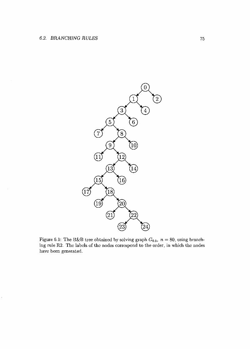
6.2. BRANCHING RULES 75
Figure 6.1: The B&B tree obtained by solving graph GO.5, n = 80, using branch-ing rule R2. The labels of the nodes correspond to the order, in which the nodeshave been generated.
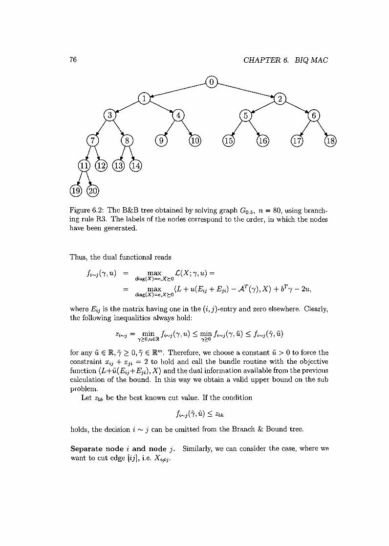
76 CHAPTER 6. BIQ MAC
Figure 6.2: The B&B tree obtained by solving graph GO.5, n = 80, using branch-ing rule R3. The labels of the nodes correspond to the order, in which the nodeshave been generated.
Thus, the dual functional reads
max L:(X;" u) =diag(X)=e,X~O
max (L + u(Eij + Eji) - ATh), X) + bT,_ 2u,diag(X)=e,X~O
where Eij is the matrix having one in the (i, j)-entry and zero elsewhere. Clearly,the following inequalities always hold:
for any u E 1R,1';:::0,1' E IRm. Therefore, we choose a constant u > 0 to force theconstraint Xij + Xji = 2 to hold and call the bundle routine with the objectivefunction (L+u(Eij+Eji), X) and the dual information available from the previouscalculation of the bound. In this way we obtain a valid upper bound on the subproblem.
Let Zbk be the best known cut value. If the condition
holds, the decision i rv j can be omitted from the Branch & Bound tree.
Separate node i and node j. Similarly, we can consider the case, where wewant to cut edge [ij], i.e. Xifj.
6.3. IMPLEMENTATION OF THE BIQ MAC SOLVER 77
How to use strong branching. We consider two different variants of incor-porating strong branching.
First R2J then R3. First, find the 6 'best' potential branching edges accordingto rule R2. These are edges, where we expect to be able to cut off one of thesub trees quickly. We do a quick forecast on each of these branching decisionsand hope to be able to fathom this node (before we actually add it), i.e. we onlyhave to add one node to the branching tree. If we do not succeed in finding suchan edge, we do a forecast on the 6 'best' branching edges according to rule R3and branch then on the edge, where the decrease of the bound in both childrenis maximal.
R3 only. Do a forecast on the 6 'best' branching edges of rule R3. Branch onthe edge, where the largest decrease of the bound in both children is expected.
Performance. It was disappointing to see, that strong branching does notseem to be worth the effort. There was only a slight decrease in the numberof nodes, compared to the vast increase of computation time. Contrary to LP,where sensitivity analysis is at hand, for Semidefinite Programming no similarresults exist and the dual information available at the end of the bundle iterationscannot be utilized. If we actually add a node to the B&B tree, that could beomitted by strong branching, the effect is, that after very little bundle iterationsthe node can be fathomed anyway.
6.3 Implementation of the Biq Mac SolverWe implemented the Branch & Bound Algorithm described above in C. For op-erations arising from linear algebra we use ATLAS (Automatically Tuned LinearAlgebra Software), which is an open source implementation of BLAS (Basic Lin-ear Algebra Subprograms) and parts of LAPACK (Linear Algebra PACKage).
To solve the SDP, which has to be done several times during the algorithm, weimplemented a predictor-corrector version of an Interior-Point Algorithm usingthe HKM-direction (see Section 1.4.1).
We did not cover yet, when to stop the bundle algorithm. Although thereis a very distinct tailing-off effect, it is not advisable to let the algorithm run,until we have reached tailing-off. The reason is, that if it is obvious, that thebounding procedure will not succeed to declare the best known feasible solutionof this node to be optimal, we do not want to waste time by calculating thebound tightly. Therefore, after some bundle iterations we make a rough forecastto decide whether it is worth doing more bundle iterations or if the gap, i.e. thedifference between the bound and the best known feasible solution, cannot beclosed anyway.
Another issue is, after how many bundle-iterations we should purge the con-straints and add newly violated ones. Let us call the bundle-iterations done
78 CHAPTER 6. BIQ MAC
between the process of purging/separating 'inner iterations' and one round of do-ing the inner iterations followed by purging and separating constraints an 'outeriteration'. At the beginning of the bundle algorithm the number of inner iter-ations should be small, say three iterations. Then this number is increased ineach outer iteration until a limit of, say ten inner iterations, is reached. This ismotivated by the fact, that in the beginning it will take a while until we havefound the 'right' set of triangle-inequalities and we do not waste time by tryinghard to push the bound down if the current set of triangle-inequalities does notallow much progress.
Experiments show that it is definitely advisable to apply these dynamic strate-gies. Using the Bundle Method as described in Section 5.1.2 in a B&B frameworkwithout these features leads to significantly longer computation times. By apply-ing the dynamic strategies, we saved up to 30% of computation time comparedto an algorithm using a static number of inner and outer iterations.
We can now summarize the algorithm, performed at each node of the B&Btree as Algorithm 6.2, with subroutines described in Algorithms 6.3 and 6.4 below.
Algorithm 6.2 (Biq Mac, algorithm performed at each node of the B&B tree)Subroutines 'function evaluation' and 'separation' can be found in Algorithms 6.3and 6.4 below.
Input.Laplace matrix L.Parameter:
itinneTl itouter, itextra, maxitinner, minitoutergaprelax = 1 if all weights are integers} otherwise gaprelax = O.branchingule} c.
Start.i=l} done=false, I= 0, l' = D.j, g, X f- function evaluation with L, 1', I.G = g,F = (L,X),X = X.I f- separation with X.Xbk, Zbk f- rounding heuristic, see Section 3.4.
repeatj, g, X f- function evaluation with L, 1', I.add this information to bundle F, G, X.j=l.while j < itinner and f + c ~ Zbk + gaprelax
Solve (5.12) and obtain À, 'Tl."(test = l' - t('Tl- GÀ), see (5.11)ftest, gtest, Xtest f- function evaluation f at "(test.
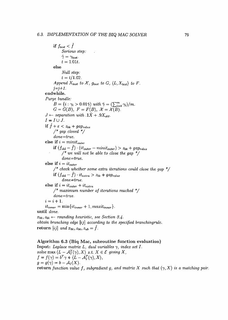
6.3. IMPLEMENTATION OF THE BIQ MAC SOLVER
if ftest < fSerious step:..y = Itest.t = 1.0It.
elseNull step:t = t/1.02.
Append Xtest to X, gtest to G, (L,Xtest) to F.j=j+1.
endwhile.Purge bundle:
B = {i : Ii > 0.011') with l' = O::z:,11i)/m.G = G(B), F = F(B), X = X(B).
J f- separation with .1X + .9Xold'1= lU J.if j + E < Zbk + gaprelax
j* gap closed *jdone=true.
else if i = minitouterif (fold - j) . (itouter - minitouter) > Zbk + gaprelax
j* we will not be able to close the gap *jdone=true.
else if i = itouterj* check whether some extra iterations could close the gap *jif (fold - j) . itextra > Zbk + gaprelax
done=true.else if i = itouter + itextra
j* maximum number of iterations reached *jdone=true.
i=i+1.itinner = min {itinner + 1, maxitinner}.
until done.Xbk, Zbk f- rounding heuristic, see Section 3.4.obtain branching edge [ij] according to the specified branchingrule.return [ij] and Xbk, Zbk, Zub = j.
79
Algorithm 6.3 (Biq Mac, subroutine function evaluation)Input: Laplace matrix L, dual variables l, index set l.solve max (L - Afb), X) s.t. X E £ giving X,f = fb) = bTI + (L - Afb),X),g = gb) = b - A1(X).return function value f, subgradient g, and matrix X such that b,X) is a matching pair.
80 CHAPTER 6. BIQ MAC
Algorithm 6.4 (Biq Mac, subroutine separation)Input.
Matrix X.Parameter heapsize, maxgentri, mandatorYtri
Create a heap of size 'heapsize' with those triangle-inequalities violatedmost by X.I f- indices of the mandatorYtr most violated ones.Choose randomly (max gen - mandatorYtr) triangle-inequalities fromthe remaining heap and add it to I.return indices I of new constraints.
In Figure 6.3 we present a typical call-graph of solving some instance. mainis the program that administrates the B&B tree and calls the bounding proce-dure. In bound the bundle-routine is called and the branching-edge is determined.bdLlIlain calls the heuristic, starts the bundle-iterations and also separation andpurging of the triangles are done in this program. Note, that the heuristic-routineas well as the separation-routine takes so little time (less than 2% each), thatthey are not displayed in this call-graph. The 'inner' bundle iterations are donein bdLlllC2, here also the routine doing the function evaluation fct_eval andthe routine lam_eta for solving the À-1]-problem(5.12) are invoked. Solving theSDP in order to evaluate the function is done in mc_psdpk. The other routines inthe graph are doing linear algebra operations, like matrix multiplications, matrixinversion, cholesky factorization, etc.
Since the programs of our interest are only the top-level routines, we zoomin Figure 6.4 into the top 11 sub-programs. We see that program mcpsdpk,which solves the SDP, uses up 88% of the overall time, whereas time for solvingthe À-1]-problem,solving the heuristic, and doing separation is negligible. Thismeans, the best way of saving computation time, is trying to keep the number offunction evaluations small. For this reason we choose the number of inner andouter iterations dynamically, as described above.
6.4 The Biq Mac LibraryWe have collected a wide variety of test problems of both, (MC) and (QP).All the data sets together with a description can be downloaded from http: / /www.math.uni-klu.ac.at/or/Software. The instances are taken from varioussources, here we provide the characteristics of the data sets and references topapers where the problems are introduced and (possibly) solved. Throughout thissection n is the dimension of the graph (for (MC) instances) or the dimensionof matrix Q (for (QP) instances). d is the density of the graph or of matrix Q,respectively.

6.4. THE BIQ MAC LIBRARY 81
Figure 6.3: A typical call graph. Note, that the subroutine that does the separa-tion of the triangle inequalities consumes so little time, that it does not appearin this graph.
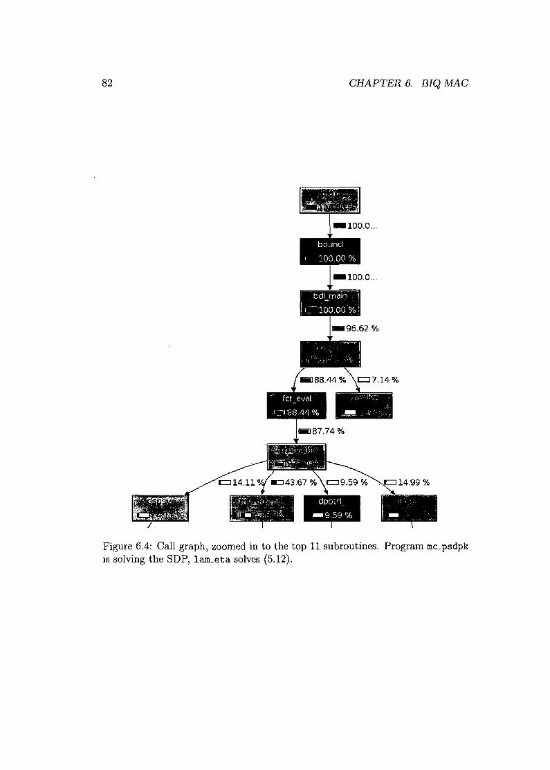
82 CHAPTER 6. BIQ MAC
--Figure 6.4: Call graph, zoomed in to the top 11 subroutines. Program mc_psdpkis solving the SDP, lam_eta solves (5.12).
6.4. THE BIQ MAC LIBRARY
6.4.1 Max-Cut
83
rudy-generated instances
The first group of instances is suggested by Helmberg and Rendl [54] and consistsof random graphs (of specified edge density) with various types of random edgeweights. All graphs were generated by the graph generator rudy of Rinaldi [116].We generated ten instances each of the following types of graphs:
• GO.5unweighted graphs with edge probability 1/2, n = 80 and n = 100.
• G-1/O/1weighted (complete) graphs with edge weights chosen uniformly from {-l,a, I}and density d = 0.1 and d = 0.99, n = 100.
• G[-lO,lO]Graphs with integer edge weights chosen from [-10,10] and density d = 0.5and d = 0.9, n = 100.
• G[O,lOlGraphs with integer edge weights chosen from [-la, la] and density d = 0.5and d = 0.9, n = 100.
Applications in physics: Ising instances
We also consider a set of test-problems from F. Liers [personal communication,Dec. 2005] deduced from physical applications. There are two kind of instances:
• two- and three-dimensional grid graphs, with Gaussian-distributed weights(zero mean and variance one). We select graphs of size 10 x la, 15 x 15,20 x 20, 5 x 5 x 5, 6 x 6 x 6 and 7 x 7 x 7.
• dense Ising instances (one dimensional Ising chain), i.e. complete graphswith a certain structure. These instances are obtained in the followingway: all nodes lie evenly distributed on a cycle. The weights of the edgesdepend on the Euclidean distance between two nodes and a parameter (7,
such that the following proportion holds:
€ijCi' rv -
J rf!.tJ
where €ij is chosen according to a Gaussian distribution with zero meanand variance one and rij is the Euclidean distance between nodes i and j.The graphs we have chosen are of size n E {lOa, 150,200,250, 300}.
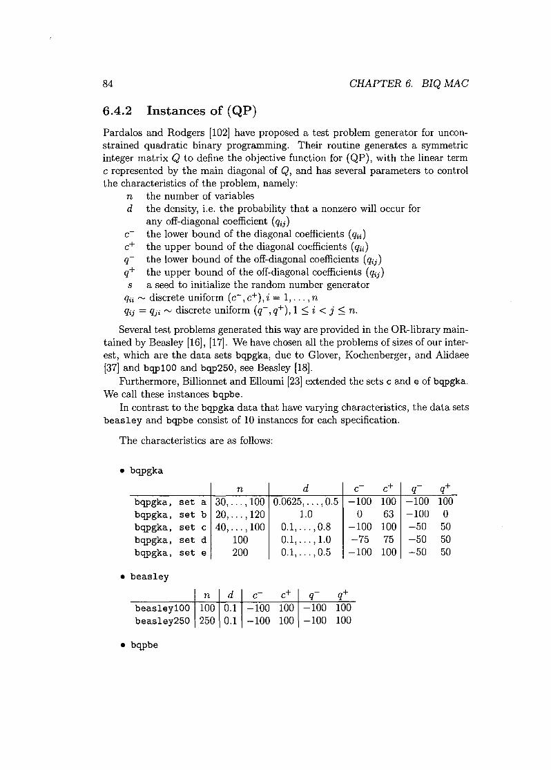
84 CHAPTER 6. BIQ MAC
6.4.2 Instances of (QP)Pardalos and Rodgers [102] have proposed a test problem generator for uncon-strained quadratic binary programming. Their routine generates a symmetricinteger matrix Q to define the objective function for (QP), with the linear termc represented by the main diagonal of Q, and has several parameters to controlthe characteristics of the problem, namely:
n the number of variablesd the density, i.e. the probability that a nonzero will occur for
any off-diagonal coefficient (%)c the lower bound of the diagonal coefficients (qii)c+ the upper bound of the diagonal coefficients (qii)q the lower bound of the off-diagonal coefficients (%)q+ the upper bound of the off-diagonal coefficients (%)s a seed to initialize the random number generator
qii rv discrete uniform (c-, c+), i = 1, ... , n% = %i rv discrete uniform (q-, q+), 1 :::;i < j :::;n.
Several test problems generated this way are provided in the OR-library main-tained by Beasley [16], [17]. We have chosen all the problems of sizes of our inter-est, which are the data sets bqpgka, due to Glover, Kochenberger, and Alidaee[37] and bqp100 and bqp250, see Beasley [18].
Furthermore, Billionnet and Elloumi [23]extended the sets c and e of bqpgka.We call these instances bqpbe.
In contrast to the bqpgka data that have varying characteristics, the data setsbeasley and bqpbe consist of 10 instances for each specification.
The characteristics are as follows:
• bqpgka
n d c- c+ q- q+bqpgka, set a 30, ... ,100 0.0625, ... ,0.5 -100 100 -100 100bqpgka, set b 20, ... ,120 1.0 0 63 -100 0bqpgka, set c 40, ... ,100 0.1, ... ,0.8 -100 100 -50 50bqpgka, set d 100 0.1, ... ,1.0 -75 75 -50 50bqpgka, set e 200 0.1, ... ,0.5 -100 100 -50 50
• beasley
n d c- c+ q q+beasley100 100 0.1 -100 100 -100 100beasley250 250 0.1 -100 100 -100 100
• bqpbe
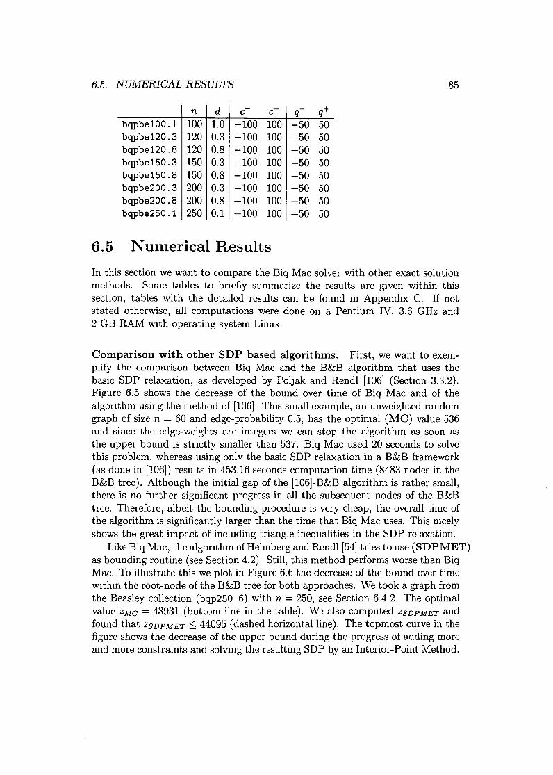
6.5. NUMERICAL RESULTS
n d c- c+ q- q+bqpbel00.l 100 1.0 -100 100 -50 50bqpbe120.3 120 0.3 -100 100 -50 50bqpbe120.8 120 0.8 -100 100 -50 50bqpbe150.3 150 0.3 -100 100 -50 50bqpbe150.8 150 0.8 -100 100 -50 50bqpbe200.3 200 0.3 -100 100 -50 50bqpbe200.8 200 0.8 -100 100 -50 50bqpbe250.1 250 0.1 -100 100 -50 50
6.5 Numerical Results
85
In this section we want to compare the Biq Mac solver with other exact solutionmethods. Some tables to briefly summarize the results are given within thissection, tables with the detailed results can be found in Appendix C. If notstated otherwise, all computations were done on a Pentium IV, 3.6 GHz and2 GB RAM with operating system Linux.
Comparison with other SDP based algorithms. First, we want to exem-plify the comparison between Biq Mac and the B&B algorithm that uses thebasic SDP relaxation, as developed by Poljak and Rendl [106] (Section 3.3.2).Figure 6.5 shows the decrease of the bound over time of Biq Mac and of thealgorithm using the method of [106]. This small example, an unweighted randomgraph of size n = 60 and edge-probability 0.5, has the optimal (MC) value 536and since the edge-weights are integers we can stop the algorithm as soon asthe upper bound is strictly smaller than 537. Biq Mac used 20 seconds to solvethis problem, whereas using only the basic SDP relaxation in a B&B framework(as done in [106]) results in 453.16 seconds computation time (8483 nodes in theB&B tree). Although the initial gap of the [106]-B&B algorithm is rather small,there is no further significant progress in all the subsequent nodes of the B&Btree. Therefore, albeit the bounding procedure is very cheap, the overall time ofthe algorithm is significantly larger than the time that Biq Mac uses. This nicelyshows the great impact of including triangle-inequalities in the SDP relaxation.
Like Biq Mac, the algorithm of Helmberg and Rendl [54]tries to use (SDPMET)as bounding routine (see Section 4.2). Still, this method performs worse than BiqMac. To illustrate this we plot in Figure 6.6 the decrease of the bound over timewithin the root-node of the B&B tree for both approaches. We took a graph fromthe Beasley collection (bqp250-6) with n = 250, see Section 6.4.2. The optimalvalue ZMC = 43931 (bottom line in the table). We also computed ZSDPMET andfound that ZSDPMET :s: 44095 (dashed horizontalline). The topmost curve in thefigure shows the decrease of the upper bound during the progress of adding moreand more constraints and solving the resulting SDP by an Interior-Point Method.

86
55
Q)=>ëij>
B 545I
)(t'IlE
"Cc:t'IlCIl"Cc:=>o.0
~ 540a.=>
CHAPTER 6. BIQ MAC
535o 5 10 15 20 25 30computation time in seconds
35 40
Figure 6.5: Solving an instance of GO.5, n = 60, with the B&B algorithm intro-duced by Poljak and Rendl [106] (line above) and Biq Mac. Optimal solution ofBiq Mac after 20 seconds, [106] takes 453.16 seconds.
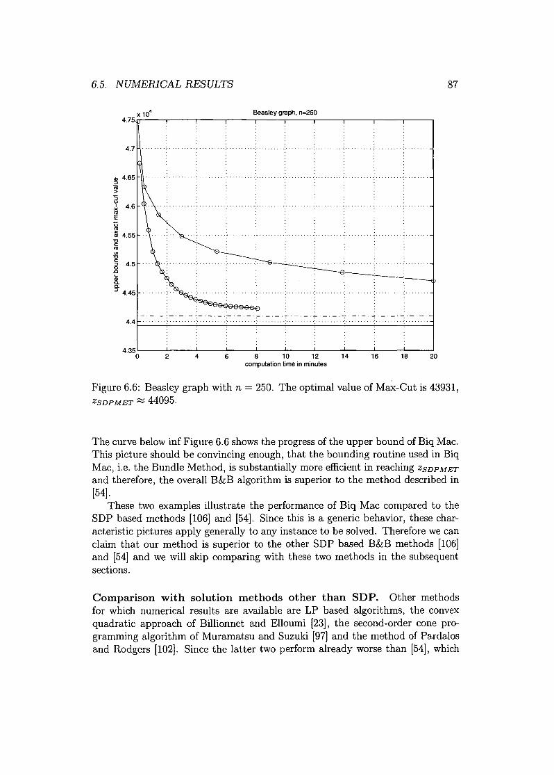
6.5. NUMERICAL RESULTS
X 10'4.75
4.7
Beasley graph, n=250
. .............
87
CIl 4.65:::l(ij>:;(.)
~ 4.6
~Ü<11~ 4.55uc:<11
'"Uc::::lo.0Q;e.e.:::l 4.45
4.4. . . .-,-.-.-.-.-'-.-.-.-.-.-. . . .
.............. . - .
4.35o 2 4 6 8 10 12 14computation time in minutes
16 18 20
Figure 6.6: Beasley graph with n = 250. The optimal value of Max-Cut is 43931,ZSDPMET:::::: 44095.
The curve below inf Figure 6.6 shows the progress of the upper bound of Biq Mac.This picture should be convincing enough, that the bounding routine used in BiqMac, i.e. the Bundle Method, is substantially more efficient in reaching ZSDPMET
and therefore, the overall B&B algorithm is superior to the method described in[54].
These two examples illustrate the performance of Biq Mac compared to theSDP based methods [106] and [54]. Since this is a generic behavior, these char-acteristic pictures apply generally to any instance to be solved. Therefore we canclaim that our method is superior to the other SDP based B&B methods [106]and [54] and we will skip comparing with these two methods in the subsequentsections.
Comparison with solution methods other than SDP. Other methodsfor which numerical results are available are LP based algorithms, the convexquadratic approach of Billionnet and Elloumi [23], the second-order cone pro-gramming algorithm of Muramatsu and Suzuki [97] and the method of Pardalosand Rodgers [102]. Since the latter two perform already worse than [54], which
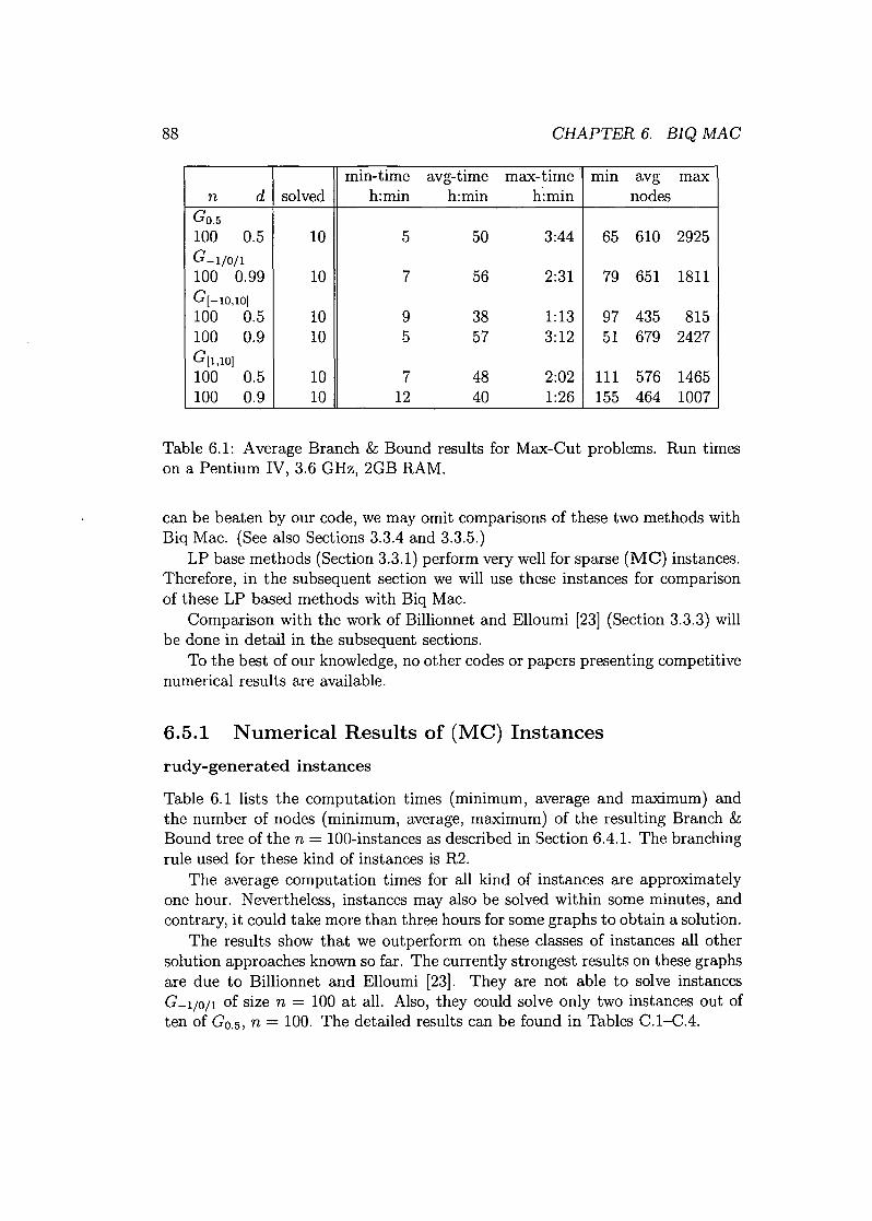
88 CHAPTER 6. BIQ MAC
min-time avg-time max-time mm avg maxn d solved h:min h:min h':min nodes
GO.5
100 0.5 10 5 50 3:44 65 610 2925G-1/O/1
100 0.99 10 7 56 2:31 79 651 1811G[-lO,lOj100 0.5 10 9 38 1:13 97 435 815100 0.9 10 5 57 3:12 51 679 2427G[l,lOj100 0.5 10 7 48 2:02 111 576 1465100 0.9 10 12 40 1:26 155 464 1007
Table 6.1: Average Branch & Bound results for Max-Cut problems. Run timeson a Pentium IV, 3.6 GHz, 2GB RAM.
can be beaten by our code, we mayomit comparisons of these two methods withBiq Mac. (See also Sections 3.3A and 3.3.5.)
LP base methods (Section 3.3.1) perform very well for sparse (MC) instances.Therefore, in the subsequent section we will use these instances for comparisonof these LP based methods with Biq Mac.
Comparison with the work of Billionnet and Elloumi [23] (Section 3.3.3) willbe done in detail in the subsequent sections.
To the best of our knowledge, no other codes or papers presenting competitivenumerical results are available.
6.5.1 Numerical Results of (MC) Instances
rudy-generated instances
Table 6.1 lists the computation times (minimum, average and maximum) andthe number of nodes (minimum, average, maximum) of the resulting Branch &Bound tree of the n = lOO-instances as described in Section 6.4.1. The branchingrule used for these kind of instances is R2.
The average computation times for all kind of instances are approximatelyone hour. Nevertheless, instances mayalso be solved within some minutes, andcontrary, it could take more than three hours for some graphs to obtain a solution.
The results show that we outperform on these classes of instances all othersolution approaches known so far. The currently strongest results on these graphsare due to Billionnet and Elloumi [23]. They are not able to solve instancesG-1/O/1 of size n = 100 at all. Also, they could solve only two instances out often of GO.5, n = 100. The detailed results can be found in Tables o.1-CA.
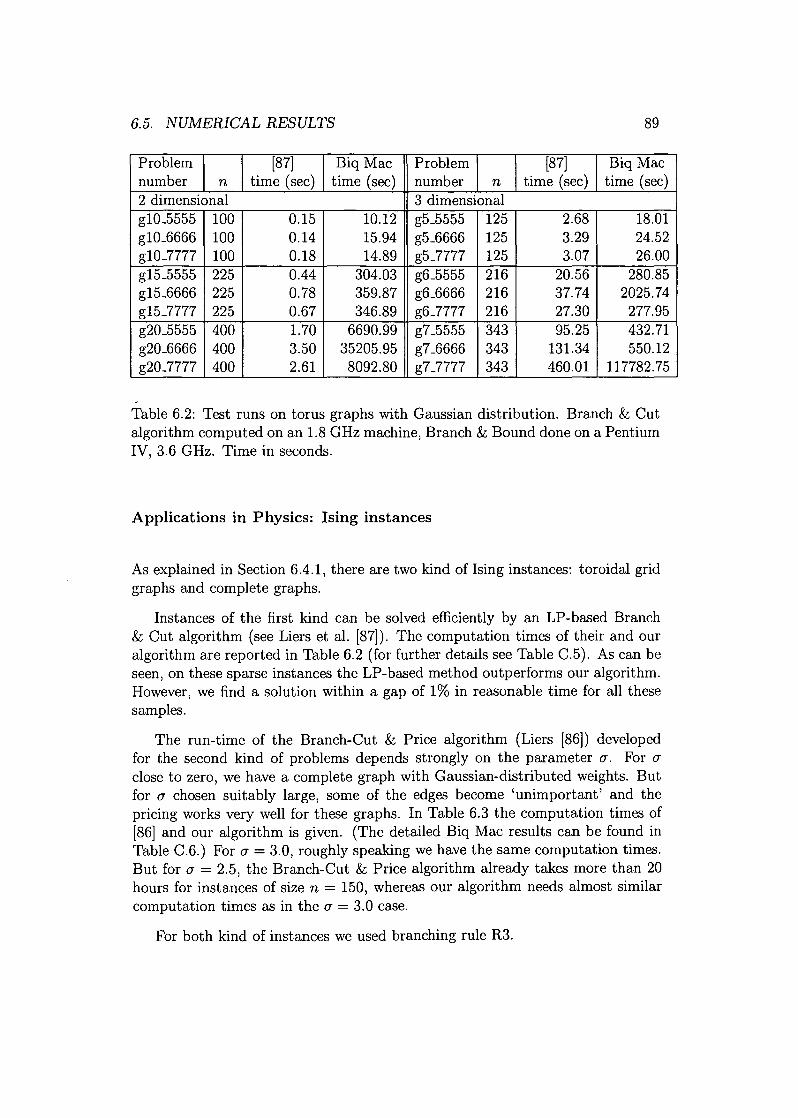
6.5. NUMERICAL RESULTS 89
Problem [87] Biq Mac Problem [87] Biq Macnumber n time (sec) time (sec) number n time (sec) time (sec)2 dimensional 3 dimensionalglO_5555 100 0.15 10.12 g5_5555 125 2.68 18.01g10_6666 100 0.14 15.94 g5_6666 125 3.29 24.52g10-7777 100 0.18 14.89 g5_7777 125 3.07 26.00g15_5555 225 0.44 304.03 g6_5555 216 20.56 280.85g15_6666 225 0.78 359.87 g6_6666 216 37.74 2025.74g15-7777 225 0.67 346.89 g6-7777 216 27.30 277.95g20_5555 400 1.70 6690.99 g7_5555 343 95.25 432.71g20_6666 400 3.50 35205.95 g7_6666 343 131.34 550.12g20-7777 400 2.61 8092.80 g7-7777 343 460.01 117782.75
Table 6.2: Test runs on torus graphs with Gaussian distribution. Branch & Cutalgorithm computed on an 1.8 GHz machine, Branch & Bound done on a PentiumIV, 3.6 GHz. Time in seconds.
Applications in Physics: Ising instances
As explained in Section 6.4.1, there are two kind of Ising instances: toroidal gridgraphs and complete graphs.
Instances of the first kind can be solved efficiently by an LP-based Branch& Cut algorithm (see Liers et al. [87]). The computation times of their and ouralgorithm are reported in Table 6.2 (for further details see Table C.5). As can beseen, on these sparse instances the LP-based method outperforms our algorithm.However, we find a solution within a gap of 1% in reasonable time for all thesesamples.
The run-time of the Branch-Cut & Price algorithm (Liers [86]) developedfor the second kind of problems depends stronglyon the parameter (}". For (}"close to zero, we have a complete graph with Gaussian-distributed weights. Butfor (}"chosen suitably large, some of the edges become 'unimportant' and thepricing works very well for these graphs. In Table 6.3 the computation times of[86] and our algorithm is given. (The detailed Biq Mac results can be found inTable C.6.) For (}"= 3.0, roughly speaking we have the same computation times.But for (}"= 2.5, the Branch-Cut & Price algorithm already takes more than 20hours for instances of size n = 150, whereas our algorithm needs almost similarcomputation times as in the (}"= 3.0 case.
For both kind of instances we used branching rule R3.

90 CHAPTER 6. BIQ MAC
Problem [86] Biq Mac Problem [86] Biq Macnumber n h:min:sec h:min:sec number n h:min:sec h:min:sec
(J = 3.0 (J = 2.5100_5555 100 4:52 1:36 100_5555 100 18:22 1:32100_6666 100 0:24 0:34 100_6666 100 6:27 1:061003777 100 7:31 0:48 1003777 100 10:08 0:47150_5555 150 2:36:46 4:38 150_5555 150 21:28:39 4:25150_6666 150 4:49:05 3:55 150_6666 150 23:35:11 5:391503777 150 3:48:41 6:06 1503777 150 31:40:07 9:19200_5555 200 9:22:03 10:07 200_5555 200 - 10:05200_6666 200 32:48:03 18:53 200_6666 200 - 17:552003777 200 8:53:26 22:42 2003777 200 - 21:3825015555 250 21:17:07 1:46:29 250_5555 250 - 3:00:28250_6666 250 7:42:25 15:49 250_6666 250 - 1:17:04
. 2503777 250 17:30:13 57:24 250_7777 250 - 1:10:50300_5555 300 17:20:54 2:20:14 300_5555 300 - 6:43:47300_6666 300 10:21:40 1:32:22 300_6666 300 - 9:04:383003777 300 18:33:49 3:12:13 3003777 300 - 13:00:10
Table 6.3: Test runs on Ising instances (complete graphs). Branch-Cut & Pricecomputed on a 1.8 GHz Machine, Branch & Bound on a 3.6 GHz PC. Times inhours: minu tes:seconds.
6.5. NUMERICAL RESULTS
6.5.2 Numerical Results of (QP) Instances
91
In this section we report the results for the instances derived from (QP). Bestknown lower and upper bounds for bqpgka and beasley data are reported at thepseudo-Boolean website maintained by Boros, Hammer, and Tavares [25]. Ourresults can be found in Tables C.7-C.12, summarized we obtain the following:
• bqpgka.
- Set a. All problems are solved in the root node of the Branch &Bound tree within seconds.
Set b. These instances could all be solved, but were extremely chal-lenging for our algorithm. The reason is, that the objective value inthe Max-Cut formulation is of magnitude 106, and therefore even arelative gap of 0.1% does not allow to fathom the node. However,allowing a relative gap of 0.1%, we can solve all problems in the rootnode .of the Branch & Bound tree.
- Set c. Similar to a, also these instances were solved within someseconds in the root node of the Branch & Bound tree.
- Set d. The problems of set d could be solved within at most 7 minutes.
- Set e. The instances with 10, 20, 30 and 40% density could all besolved within 2 hours of computation time. The 50% instance hasbeen solved after 35 hours. According to [25],these problems have notbeen solved before .
• beasley.
Solving the 10 problems of size n = 100can be done in the root node withinone minute. Regarding the n = 250 instances, two out of the ten problemshave been solved before (see [25]), for the other eight problems we couldprove optimality for the first time. Six out of these eight were solved within5 hours, the other two needed 15 and 80 hours, respectively .
• bqpbe.
We report the results of Billionnet and Elloumi [23] and our results inTable 6.4. As is shown in this table, [23] could not solve all out of theten problems from the n = 120 variables and 80% density instances on,whereas our method still succeeded to solve them all. From the instancesn = 150,d = 80% on, the convex-quadratic approach failed to solve anyinstance within their time limit of 3 hours. We still managed to obtainsolutions to all of these instances (although for one graph it took 54 hours).
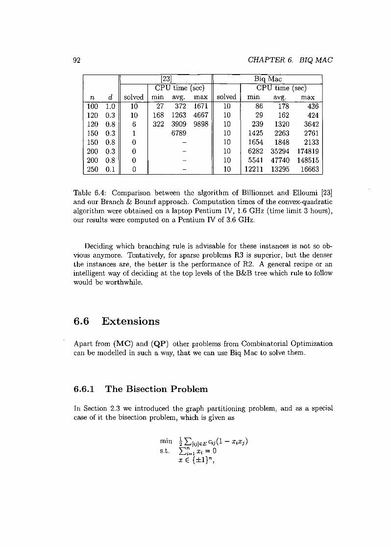
92 CHAPTER 6. BIQ MAC
[23] Biq MacCPU time (sec) CPU time (sec)
n d solved mm avg. max solved mm avg. max100 1.0 10 27 372 1671 10 86 178 436120 0.3 la 168 1263 4667 la 29 162 424120 0.8 6 322 3909 9898 10 239 1320 3642150 0.3 1 6789 10 1425 2263 2761150 0.8 a - la 1654 1848 2133200 0.3 a - 10 6282 35294 174819200 0.8 0 - 10 5541 47740 148515250 0.1 0 - 10 12211 13295 16663
Table 6.4: Comparison between the algorithm of Billionnet and Elloumi [23]and our Branch & Bound approach. Computation times of the convex-quadraticalgorithm were obtained on a laptop Pentium IV, 1.6 GHz (time limit 3 hours),our results were computed on a Pentium IV of 3.6 GHz.
Deciding which branching rule is advisable for these instances is not so ob-vious anymore. Tentatively, for sparse problems R3 is superior, but the denserthe instances are, the better is the performance of R2. A general recipe or anintelligent way of deciding at the top levels of the B&B tree which rule to followwould be worthwhile.
6.6 Extensions
Apart from (MC) and (QP) other problems from Combinatorial Optimizationcan be modelled in such a way, that we can use Biq Mac to solve them.
6.6.1 The Bisection Problem
In Section 2.3 we introduced the graph partitioning problem, and as a specialcase of it the bisection problem, which is given as
mm !L:[ij]EEG,;j(l- XiXj)
s.t. L:~=lXi = 0xE {:i:1}n,
6.6. EXTENSIONS 93
for a graph G = (V (G), E( G)) and edge weights Cij. By setting X := XXT, thefollowing natural semidefinite relaxation arises:
mm ~trLXs.t. trJX = a
diag(X) = eXtO,
where L is the Laplace matrix of graph Gand J is the matrix of all ones.Let A be the adjacency matrix of an unweighted graph. Solving the Max-Cut
problem of a graph with cost matrix
B = -A+ J
gives a cut 8(S) with value z. If ISI = ~ then
n2--z4
is the optimal value of the bisection problem. (The "-" in B = -A + J arises,because we do a maximization instead of minimizing, and the J comes from theconstraint tr JX = 0, that is lifted into the objective function. The Lagrangemultiplier for this constraint is guessed to be one.)
We consider the instances introduced by Johnson, Aragon, McGeoch, andSchevon [63] of size n = 124 and n = 250 and summarize in Table 6.5 the bestresults for these instances known so far (see Karisch and Rendl [65]). With ouralgorithm we could prove optimality of the known lower bounds of all instancesof size n = 124, and one of the instances of size n = 250. To the best of ourknowledge, these exact solutions were obtained for the first time. The improvedgap for the instances of size n = 250 and densities 0.02, 0.04 and 0.08 wereobtained after a time limit of 32 hours cpu-time.
6.6.2 Max-2SatIn Section 2.4 the Max-Sat problem has been introduced, and as a special caseof it Max-kSat. We consider here Max-2Sat, Le. we have Boolean variables{Xl, ... , Xn} and clauses that are the disjunction of at most two literals. Letus introduce variables {YI, ... , Yn}, with the correspondence Yi = a if Xi is false,and Yi = 1 if Xi is true. For each clause we can then form a cost coefficient in the(0-1) model by the following transformation
Xi V Xj ---t Yi + Yj - YiYj,
Xi V Xj ---t 1 - Yi + YiYj,Xi V Xj ---t 1 - YiYj.
With this correspondence every problem arising from Max-2Sat can be trans-formed to an instance of (QP)and thus solved by Biq Mac.
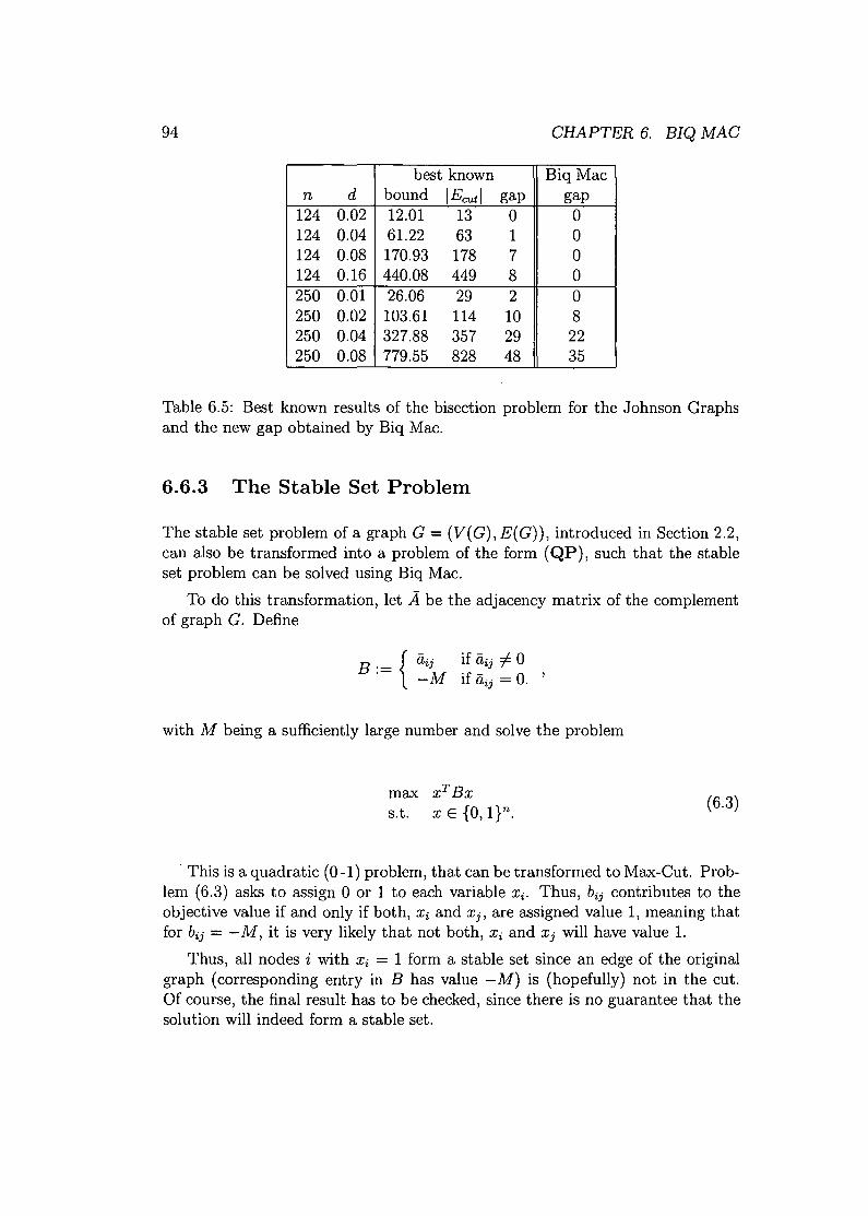
94 CHAPTER 6. BIQ MAC
best known Biq Macn d bound IEcutl gap gap
124 0.02 12.01 13 a a124 0.04 61.22 63 1 a124 0.08 170.93 178 7 a124 0.16 440.08 449 8 a250 0.01 26.06 29 2 a250 0.02 103.61 114 10 8250 0.04 327.88 357 29 22250 0.08 779.55 828 48 35
Table 6.5: Best known results of the bisection problem for the Johnson Graphsand the new gap obtained by Biq Mac.
6.6.3 The Stable Set Problem
The stable set problem of a graph G = (V(G),E(G)), introduced in Section 2.2,can also be transformed into a problem of the form (QP), such that the stableset problem can be solved using Biq Mac.
To do this transformation, let Ä be the adjacency matrix of the complementof graph G. Define
with M being a sufficiently large number and solve the problem
max xTBxS.t. x E {a, l}n . (6.3)
. This is a quadratic (0-1) problem, that can be transformed to Max-Cut. Prob-lem (6.3) asks to assign a or 1 to each variable Xi' Thus, bij contributes to theobjective value if and only if both, Xi and Xj, are assigned value 1, meaning thatfor bij = -M, it is very likely that not both, Xi and Xj will have value 1.
Thus, all nodes i with Xi = 1 form a stable set since an edge of the originalgraph (corresponding entry in B has value - M) is (hopefully) not in the cut.Of course, the final result has to be checked, since there is no guarantee that thesolution will indeed form a stable set.
6.7. CONCLUDING REMARKS ON BIQ MAC
6.6.4 The Quadratic Knapsack Problem
95
Another standard Combinatorial Optimization problem is the quadratic knapsackproblem:
(QK) max xTCxs.t. aT x:::; b
x E {a, l}n.A detailed study of this problem can be found in the book of Kellerer, Pferschy,and Pisinger [67]. Clearly, by simply providing the possibility of handling onelinear constraint, we can also solve problems of this type by Biq Mac. Incorpo-rating the possibility of having one (or even more) linear constraint(s) is part ofongoing research with C. Buchheim [personal communication, 2006].
6.7 Concluding Remarks on Biq MacThe solver Biq Mac, available via the web interface http://BiqMac .uni - klu.ac. at, solves (MC) and (QP) problems of any density up to size n = 100. To thebest of our knowledge, no other algorithm can manage these instances in a routineway. Many kind of instances of sizes up to n = 300 can be solved as well. Forthe first time optimality could be proved for several problems of the OR-library,for instance all problems that are reported at the pseudo-Boolean website [25]with dimensions up to n = 250 are now solved. Also for the bisection problemoptimality for some of the Johnson-Graphs has been proved for the first time,and for those where we could not close the gap, we reduced it significantly.
Using Biq Mac for sparse graphs is not advisable. Since linear programmingbased methods are capable of exploiting sparsity, solutions might be obtainedmuch faster when applying these methods to sparse data.
We are currently working on an extended version of Biq Mac that is capableof handling some linear constraints explicitly, which will broaden the field ofapplications. Also, having a recipe for the proper branching rule or a way ofdynamically deciding which rule to use, is work in progress.
Summary and Outlook
This thesis covers algorithms for large-scale Semidefinite Programs, as well assolution methods for the Max-Cut problem, an NP-complete problem arisingfrom Combinatorial Optimization.
We explain basic theoretical issues of Semidefinite Programs and the mostwell-known solution methods (Chapter 1). The field of Combinatorial Optimiza-tion problems is reviewed (Chapter 2) and one of the problems, namely the Max-Cut problem, is discussed in more detail in Chapter 3.
Chapter 4 addresses SDP based relaxations for Max-Cut. We introduce a newrelaxation for sparse problems where the support of the graph plays a major roleto develop the SDP-relaxation and we implemented a Bundle Method to solvethis Semidefinite Program. A topic of further investigations is to look at thepractical behavior of other sparse models that are independent of the structureof the graph.
The increasing demand of algorithms for solving large-scale SDPs motivatedthe work in Chapter 5. Apart from recalling the concept of Bundle Methods andapplying it in Semidefinite Programming, we developed a Spectral Bundle methodthat uses second order information. An implementation of this algorithm is partof ongoing work. This code should then also be capable of solving the sparserelaxation from Chapter 4 for higher dimensions. Another new algorithm intro-duced in Chapter 5 is the Boundary Point Method. The augmented Lagrangianalgorithm is the background of this method, that works astonishing well for theproblem of calculating the 'l9-numberof a graph. For solving relaxations arisingfrom other sources, the algorithm does not behave as nicely. Finding a way tomake the Boundary Point Method applicable to more problems is part of futureresearch.
In the final chapter we introduced the Biq Mac solver - a tool for solving Max-Cut (or, equivalently unconstrained binary quadratic programs) and the Biq Maclibrary - various instances arising from Max-Cut or unconstrained quadratic (a-1) programming. We made this solver publicly available via the web-site http:/ /BiqMac. uni -klu. ac. at. Also, the collection of test problems is accessible. Anongoing maintenance of this library in order to develop benchmarks for Max-Cutand unconstrained quadratic (0 -1) problems is intended.
97
Appendix A
Background Material
A.I Positive Semidefinite MatricesIn this section we state some of the definitions and theorems concerning positivesemidefinite matrices. All the proofs can be found in Horn and Johnson [61].
Theorem A.I (Characterization of positive semidefinite matrices)Let X E Sn. The following statements are equivalent .
• X t: O .
• À(X) ~ 0 for all Eigenvalues À of X .
• All principal minors of X are non-negative .
• :3L E IRnxn: X = LLT.
Lemma A.2 Any principal submatrix of a positive definite matrix is positivedefinite.
Theorem A.3 (Fejer) A E s;t if and only iftrAB ~ 0 VB E s;t
Lemma AA If A, B E s;t, then (A, B) > 0 and (A, B) - 0 if and only ifAB=O.
Observation A.5 If A E s;t and aii = 0 for some i E {I, ... ,n}, then aij =aji = 0 for all j E {I, ... ,n}.
99

100 APPENDIX A. BACKGROUND MATERIAL
Definition A.6 (Schur complement) If
where A is nonsingular and C is symmetric. Then
is called the Schur complement of A in M.
Theorem A.7 Let
M= (tT ~)
where A is positive definite and C is symmetric. Then
A.2 Convexity, Minimax InequalityDefinition A.8 (convex set) A set C ç ]Rn is convex if Cl, C2 E C impliesaCI + (1 - a)c2 E C for all a E [0,1].
Definition A.9 (convex hull) The convexhull conv(S) of some set S ç ]Rnisthe smallest convex set that contains S.
Lemma A.IO conv({vvT, Ilvll = I}) = {W ~ 0, trW = I}.
Lemma A.II (minimax inequality) [117, Lemma 36.1} Let f be a functionfrom the non-empty product set C x D to [-00,00], then
sup inf f(u,v)::; inf supf(u,v).uEC vED vED uEC
Corollary A.12 [117, Theorem 37.3) Let f be a function from the non-emptyproduct set C x D, C and D being closed convex sets in]Rm and ]Rn, respectively,to [-00,00]. If either C or D is bounded, then
sup inf f(u,v) = inf supf(u,v).UEcVED VEDuEC
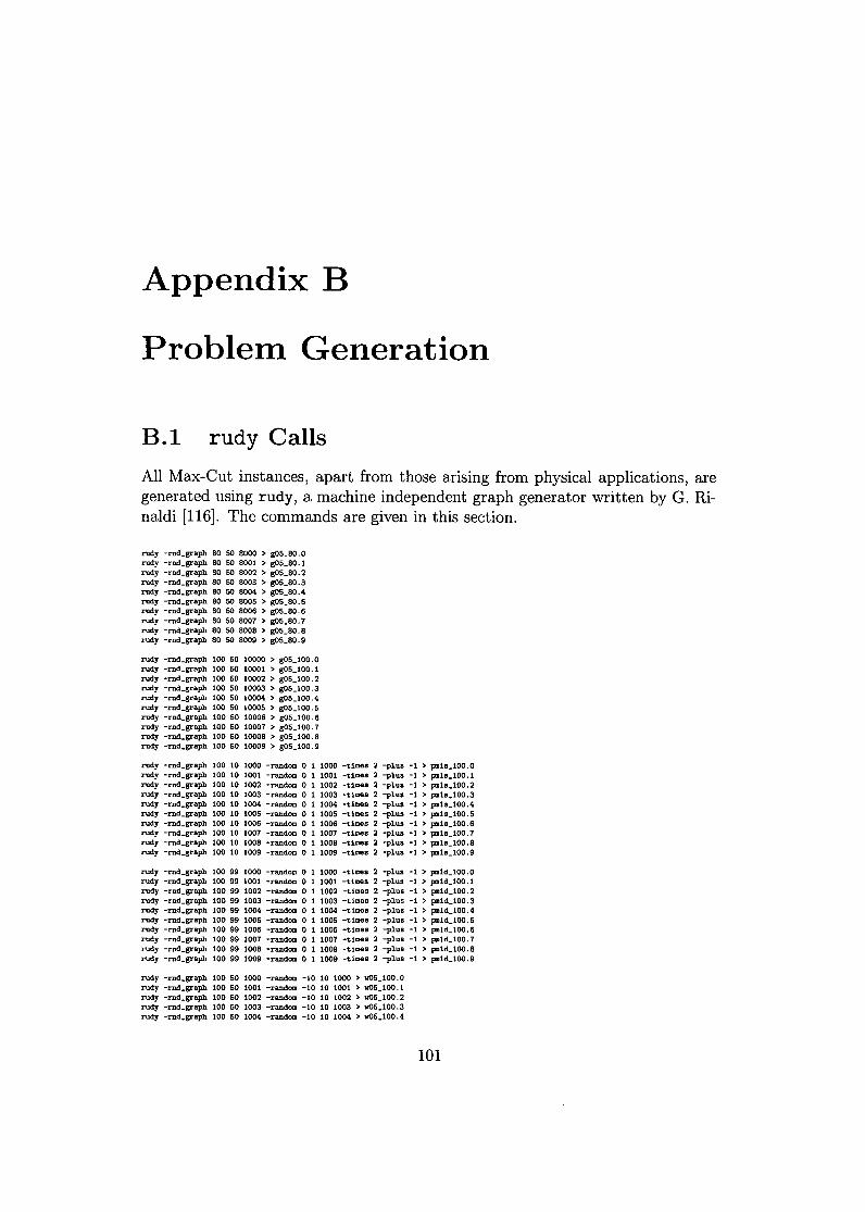
Appendix B
Problem Generation
B.l rudy CallsAll Max-Cut instances, apart from those arising from physical applications, aregenerated using rudy, a machine independent graph generator written by G. Ri-naldi [116]. The commands are given in this section.
rudy -rnd_graph 80 50 8000 > 805_80.0rudy -md_graph 80 50 8001 > 805_80.1rudy -md_graph 80 50 8002 > 805_80.2rudy -md_graph 80 50 8003 > 805_80.3rudy -md_graph 80 50 8004 > 805_80.4rudy -md_graph 80 50 8005 > 805_80.5rudy -rnd_graph 80 50 8006 > 805_80.6rudy -rnd_graph 80 50 8007 > 805_80.7rudy -md_graph 80 50 8008 > 805_80.8rudy -md_graph 80 50 8009 > 805_80.9
rudy -md_graph 100 50 10000 > 805_100.0rudy -rnd_graph 100 50 10001 > 805_100.1rudy -rnd_graph 100 50 10002 > 805_100.2rudy -md_graph 100 50 10003 > 805_100.3rudy -rnd_graph 100 50 10004 > 805_100.4rudy -rnd_graph 100 50 10005 > 805_100.5rudy -rnd_graph 100 50 10006 > 805_100.6rudy -rnd_graph 100 50 10007 > 805_100.7rudy -md_graph 100 50 10008 > 805_100.8rudy -md_graph 100 50 10009 > 805_100.9
rudy -md_graph 100 10 1000 -random 0rudy -rnd_graph 100 10 1001 -random 0rudy -rnd_graph 100 10 1002 -random 0rudy -md_graph 100 10 1003 -random 0rudy -rnd_graph 100 10 1004 -random 0rudy -rnd_graph 100 10 1005 -random 0rudy -md_graph 100 10 1006 -random 0rudy -md_graph 100 10 1007 -random 0rudy -md_graph 100 10 1008 -random 0rudy -md_graph 100 10 1009 -random 0
rudy -md_graph 100 99 1000 -random 0rudy -rnd_graph 100 99 1001 -random 0rudy -rnd_graph 100 99 1002 -random 0rudy -rnd_graph 100 99 1003 -random 0rudy -md_graph 100 99 1004 -random 0rudy -md_graph 100 99 1005 -random 0rudy -rnd_graph 100 99 1006 -random 0rudy -rnd_graph 100 99 1001 -random 0rudy -md_graph 100 99 1008 -random 0rudy -rnd_graph 100 99 1009 -random 0
1000 -times 2 -plus -1 > pIlls_IOO.a1001 -times 2 -plus -1 > pnls_l00.11002 -times 2 -pIUB -1 > pnls_100.21003 -times 2 -plus -1 > pmls_lOO. 31004 -times 2 -plus -1 > pnls_100.41005 -tlmes 2 -plus -I > ""ls_100.51006 -tlmes 2 -plus -I > ""ls_IOO. 61007 -times 2 -plus -1 > pIlls_lOO. 71008 -times 2 -plus -1 > pn18_100. 81009 -times 2 -plus -I > ""ls_IOO. 9
1000 -times 2 -plus -I > ""ld_IOO. 01001 -times 2 -plus -I > ""ld_loo.11002 -times 2 -plus -1 > pald_IOO. 21003 -tlmes 2 -plus -I > ""ld_IOO. 31004 -times 2 -plus -I > ""ld_IOO.41005 -tlmes 2 -plus -I > ""ld_IOO. 51006 -times 2 -plus -1 > pDld_l00. 61007 -times 2 -pIUB -1 > pald_IOO. 71008 -tlmes 2 -plus -I > ""Id_loo. 81009 -times 2 -plus -I > ""Id_loo. 9
rudy -rnd_graph 100 50 1000 -random -10 iO 1000 > ..05_100.0rudy -md_graph 100 50 1001 -random -10 iO 1001 > ..05_100.1rudy -md_graph 100 50 1002 -random -10 10 1002 > ..05_100.2rudy -md_graph 100 50 1003 -random -10 10 1003 > ..05_100.3rudy -md_graph 100 50 1004 -random -10 10 1004 > ..05_100.4
101
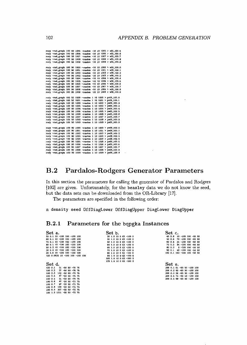
102 APPENDIX B. PROBLEM GENERATION
rudy -md_graph 100 50 1005 -random -10 10 1005 > ..05_100.5rudy -md_graph 100 50 1006 -random -10 10 1006 > ..05_100.6rudy -md_graph 100 50 1007 -random -10 10 1007 > ..05_100.7rudy -md_graph 100 50 1008 -random -10 10 1008 > ..05_100.8rudy -md_graph 100 50 1009 -random -10 10 1009 > ..05_100.9
rudy -md_graph 100 90 1000 -random -10 10 1000 > ..09_100.0rudy -md_graph 100 90 1001 -random -10 10 1001 > ..09_100.1rudy -md_graph 100 90 1002 -random -10 10 1002 > ..09_100.2rudy -md_graph 100 90 1003 -random -10 10 1003 > ..09_100.3rudy -md_graph 100 90 1004 -random -10 10 1004 > ..09_100.4rudy -md_graph 100 90 1005 -random -10 10 1005 > ..09_100.5rudy -rod_graph 100 90 1006 -random -10 10 1006 > ..09_100.6rudy -md_graph 100 90 1007 -random -10 10 1007 > ..09_100.7rudy -md_graph 100 90 1008 -random -10 10 1008 > ..09_100.8rudy -md-sraph 100 90 1009 -random -10 10 1009 > ..09_100.9
rudy -rod_graph 100 50 1000 -random 1 10 1000 > p..o5_100.0rudy -md_graph 100 50 1001 -random 1 10 1001 > p..o5_100.1rudy -md_graph 100 50 1002 -random 1 10 1002 > p..o5_100. 2rudy -md_graph 100 50 1003 -random 1 10 1003 > p..o5_100.3rudy -rod_graph 100 50 1004 -random 1 10 1004 > p..o5_100.4rudy -md_graph 100 50 1005 -random 1 10 1005 > p..o5_100. 5rudy -md_graph 100 50 1006 -random 1 10 1006 > pv05_100.6rudy -md_graph 100 50 1007 -random 1 10 1007 > p..o5_100.7rudy -rod_graph 100 50 1008 -random 1 10 1008 > p..o5_100. 8rudy -rod-sraph 100 50 1009 -random 1 10 1009 > p..o5_100. 9
rudy -md_graph 100 90 1000 -random 1 10 1000 > pw09_100.0rudy -rod_graph 100 90 1001 -random 1 10 1001 > p..o9_l00.lrudy -rod_graph 100 90 1002 -random 1 10 1002 > pw09_100.2rudy -md-sraph 100 90 1003 -random 1 10 1003 > pw09_100.3rudy -rod_graph 100 90 1004 -random 1 10 1004 > pw09_100.4rudy -rod_graph 100 90 1005 -random 1 10 1005 > pw09_100.5rudy -md_graph 100 90 1006 -random 1 10 1006 > p..o9_100.6rudy -rod_graph 100 90 1007 -random 1 10 1007 > pw09_100.7rudy -md_graph 100 90 1008 -random 1 10 1008 > pw09_100.8rudy -rod_graph 100 90 1009 -random 1 10 1009 > pw09_100.9
B.2 Pardalos-Rodgers Generator ParametersIn this section the parameters for calling the generator of Pardalos and Rodgers[102] are given. Unfortunately, for the beasley data we do not know the seed,but the data sets can be downloaded from the OR-Library [17].
The parameters are specified in the following order:
n density seed OffDiagLower OffDiagUpper DiagLower DiagUpper
Set a.50 0.1 10 -100 100 -100 10060 0.1 10 -100 100 -100 10070 0.1 10 -100 100 -100 10080 0.1 10 -100 100 -100 10050 0.2 10 -100 100 -100 10030 0.4 10 -100 100 -100 10030 0.5 10 -100 100 -100 100100 0.0625 10 -100 100 -100 100
c.40 0.8 10 -100 100 -50 5050 0.6 70 -100 100 -50 5060 0.4 31 -100 100 -50 5070 0.3 34 -100 100 -50 5080 0.2 8 -100 100 -50 5090 0.1 80 -100 100 -50 50
100 0.1 142 -100 100 -50 50
Parameters for the bqpgka Instances
Set b. Set20 1.0 10 0 63 -100 030 1.0 10 0 63 -100 040 1.0 10 0 63 -100 050 1.0 10 0 63 -100 060 1.0 10 0 63 -100 070 1.0 10 0 63 -100 080 1.0 10 0 63 -100 090 1.0 10 0 63 -100 0
100 1.0 10 0 63 -100 0125 1.0 10 0 63 -100 0
B.2.!
Set d.100 0.1 31 -50 50 -75 75100 0.2 37 -50 50 -75 75100 0.3 143 -50 50 -75 75100 0.4 47 -50 50 -75 75100 0.5 31 -50 50 -75 75100 0.6 47 -50 50 -75 75100 0.7 97 -50 50 -75 75100 0.8 133 -50 50 -75 75100 0.9 307 -50 50 -75 75100 1.0 1311 -50 50 -75 75
Set e.200 0.1 51 -50 50 -100 100200 0.2 43 -50 50 -100 100200 0.3 34 -50 50 -100 100200 0.4 73 -50 50 -100 100200 0.5 89 -50 50 -100 100
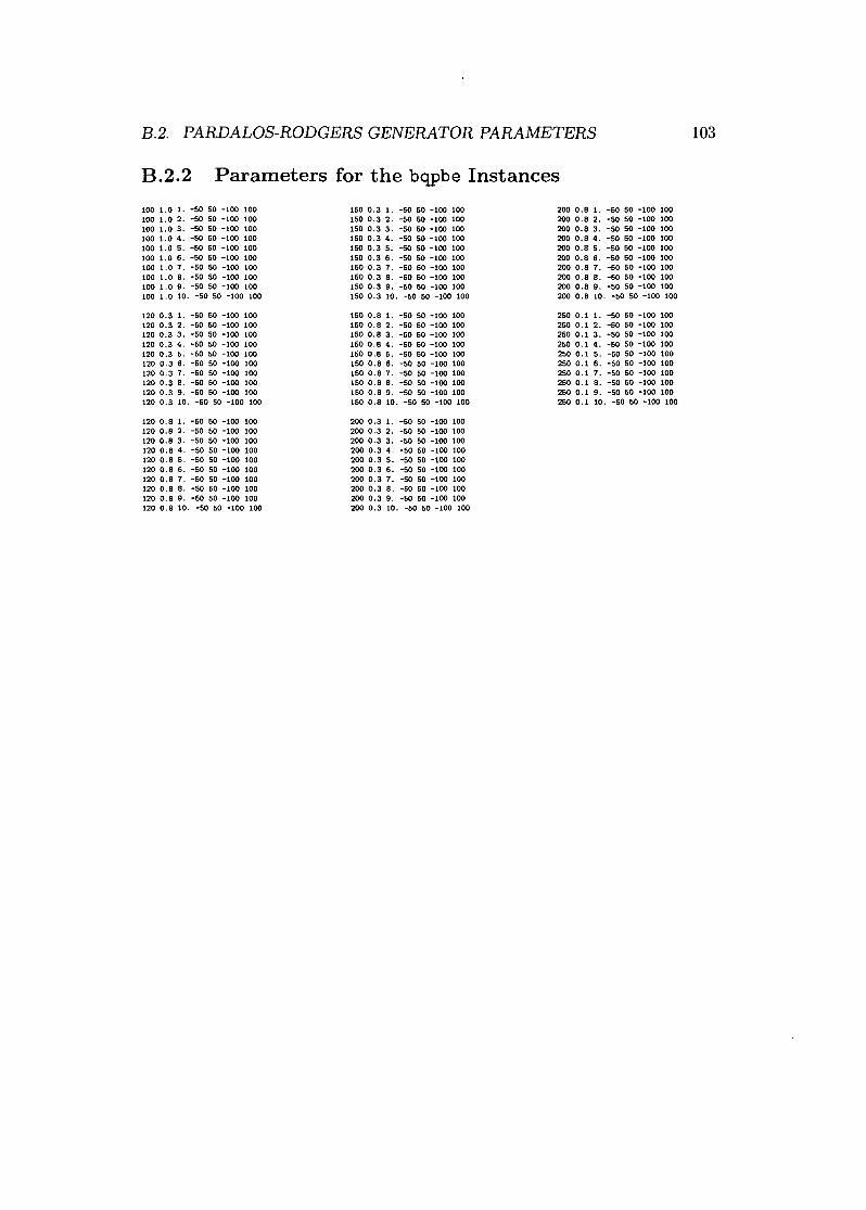
B.2. PARDALOS-RODGERS GENERATOR PARAMETERS
B.2.2 Parameters for the bqpbe Instances100 1.0 1. -50 50 -100 100 150 0.3 1. -50 50 -100 100 200 0.8 1. -50 50 -100 100100 1.0 2. -50 50 -100 100 150 0.3 2. -50 50 -100 100 200 0.8 2. -50 50 -100 100100 1.0 3. -50 50 -100 100 1500.3 3. -50 50 -100 100 200 0.8 3. -50 50 -100 100100 1.0 4. -50 50 -100 100 150 0.3 4. -50 50 -100 100 200 0.8 4. -50 50 -100 100100 1.0 5. -50 50 -100 100 150 0.3 5. -50 50 -100 100 200 0.8 5. -50 50 -100 100100 1.0 6. -50 50 -100 100 150 0.3 6. -50 50 -100 100 200 0.8 6. -50 50 -100 100100 1.07. -50 50 -100 100 1500.37. -50 50 -100 100 2000.87. -50 50 -100 100100 1.0 8. -50 50 -100 100 150 0.3 8. -50 50 -100 100 200 0.8 8. -50 50 -100 100100 1.0 9. -50 50 -100 100 150 0.3 9. -50 50 -100 100 200 0.8 9. -50 50 -100 100100 1.0 10. -50 50 -100 100 150 0.3 10. -50 50 -100 100 200 0.8 10. -50 50 -100 100
120 0.3 1. -50 50 -100 100 150 0.8 1. -50 50 -100 100 250 0.1 1. -50 50 -100 100120 0.3 2. -50 50 -100 100 150 0.8 2. -50 50 -100 100 250 0.1 2. -50 50 -100 100120 0.3 3. -50 50 -100 100 150 0.8 3. -50 50 -100 100 250 0.1 3. -50 50 -100 100120 0.3 4. -50 50 -100 100 150 0.8 4. -50 50 -100 100 2500.1 4. -50 50 -100 100120 0.3 5. -50 50 -100 100 150 0.8 5. -50 50 -100 100 250 0.1 5. -50 50 -100 100120 0.3 6. -50 50 -100 100 150 0.8 6. -50 50 -100 100 250 0.1 6. -50 50 -100 1001200.37. -50 50 -100 100 1500.87. -50 50 -100 100 250 0.1 7. -50 50 -100 100120 0.3 8. -50 50 -100 100 150 0.8 8. -50 50 -100 100 250 0.1 8. -50 50 -100 100120 0.3 9. -50 50 -100 100 150 0.8 9. -50 50 -100 100 250 0.1 9. -50 50 -100 100120 0.3 10. -50 50 -100 100 150 0.8 10. -50 50 -100 100 250 0.1 10. -50 50 -100 100
120 0.8 1. -50 50 -100 100 200 0.3 1. -50 50 -100 100120 0.8 2. -50 50 -100 100 200 0.3 2. -50 50 -100 100120 0.8 3. -50 50 -100 100 200 0.3 3. -50 50 -100 100120 0.8 4. -50 50 -100 100 200 0.3 4. -50 50 -100 100120 0.8 5. -50 50 -100 100 200 0.3 5. -50 50 -100 100120 0.8 6. -50 50 -100 100 200 0.3 6. -50 50 -100 1001200.87. -50 50 -100 100 2000.37. -50 50 -100 100120 0.8 8. -50 50 -100 100 200 0.3 8. -50 50 -100 100120 0.8 9. -50 50 -100 100 200 0.3 9. -50 50 -100 100120 0.8 10. -50 50 -100 100 200 0.3 10. -50 50 -100 100
103

104 APPENDIX B. PROBLEM GENERATION

Appendix C
Tables with Detailed NumericalResults
This chapter presents the detailed numerical results. For each instance collectedin the Biq Mac library, we tried solving the problem using both branching rulesand list in the subsequent tables the solution times in seconds and the numberof Branch & Bound nodes. All calculations were done on a Pentium IV with 3.6GHz and 2GB RAM, operating system Linux.
If no run-time is given, the problem could not be solved within a time limit of50 hours CPU-time. Instance bqp250-8 was the only one of the bqp250 instancesthat could not be solved within 50 hours. Therefore, we suspended the time limitfor this instance and could solve it within 80 hours CPU-time.
105
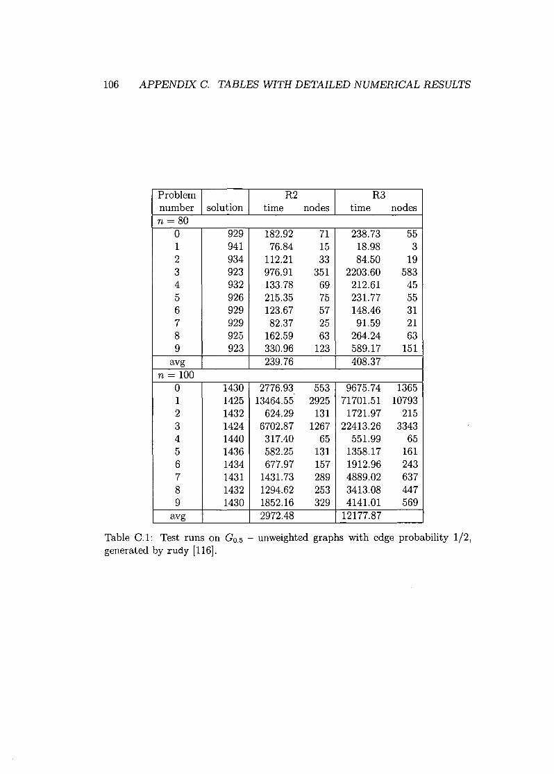
106 APPENDIX C. TABLES WITH DETAILED NUMERICAL RESULTS
Problem R2 R3number solution time nodes time nodesn = 80
a 929 182.92 71 238.73 551 941 76.84 15 18.98 32 934 112.21 33 84.50 193 923 976.91 351 2203.60 5834 932 133.78 69 212.61 455 926 215.35 75 231.77 556 929 123.67 57 148.46 317 929 82.37 25 91.59 218 925 162.59 63 264.24 639 923 330.96 123 589.17 151
avg 239.76 408.37n = 100
a 1430 2776.93 553 9675.74 13651 1425 13464.55 2925 71701.51 107932 1432 624.29 131 1721.97 2153 1424 6702.87 1267 22413.26 33434 1440 317.40 65 551.99 655 1436 582.25 131 1358.17 1616 1434 677.97 157 1912.96 2437 1431 1431.73 289 4889.02 6378 1432 1294.62 253 3413.08 4479 1430 1852.16 329 4141.01 569
avg 2972.48 12177.87
Table C.1: Test runs on GO.5 - unweighted graphs with edge probability 1/2,generated by rudy [116].
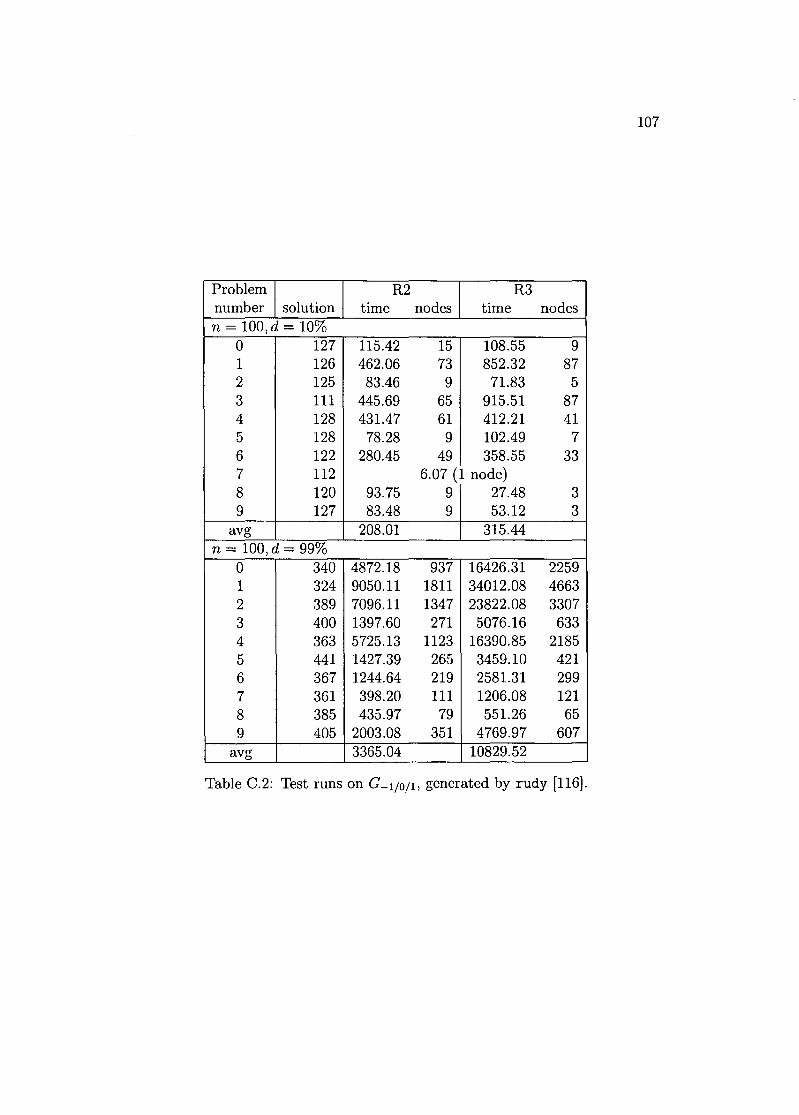
Problem R2 R3number solution time nodes time nodesn = 100,d = 10%
0 127 115.42 15 108.55 91 126 462.06 73 852.32 872 125 83.46 9 71.83 53 111 445.69 65 915.51 874 128 431.47 61 412.21 415 128 78.28 9 102.49 76 122 280.45 49 358.55 337 112 6.07 (1 node)8 120 93.75 9 27.48 39 127 83.48 9 53.12 3
avg 208.01 315.44n = 100,d = 99%
0 340 4872.18 937 16426.31 22591 324 9050.11 1811 34012.08 46632 389 7096.11 1347 23822.08 33073 400 1397.60 271 5076.16 6334 363 5725.13 1123 16390.85 21855 441 1427.39 265 3459.10 4216 367 1244.64 219 2581.31 2997 361 398.20 111 1206.08 1218 385 435.97 79 551.26 659 405 2003.08 351 4769.97 607
avg 3365.04 10829.52
Table C.2: Test runs on G-1/O/1, generated by rudy [116].
107
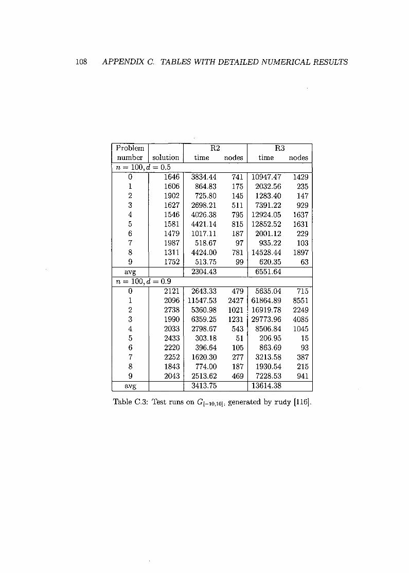
108 APPENDIX C. TABLES WITH DETAILED NUMERICAL RESULTS
Problem R2 R3number solution time nodes time nodesn = 100,d = 0.5
0 1646 3834.44 741 10947.47 14291 1606 864.83 175 2032.56 2352 1902 725.80 145 1283.40 1473 1627 2698.21 511 7391.22 9294 1546 4026.38 795 12924.05 16375 1581 4421.14 815 12852.52 16316 1479 1017.11 187 2001.12 2297 1987 518.67 97 935.22 1038 1311 4424.00 781 14528.44 18979 1752 513.75 99 620.35 63
avg 2304.43 6551.64n = 100, d = 0.9
0 2121 2643.33 479 5635.04 7151 2096 11547.53 2427 61864.89 85512 2738 5360.98 1021 16919.78 22493 1990 6359.25 1231 29773.96 40854 2033 2798.67 543 8506.84 10455 2433 303.18 51 206.95 156 2220 396.64 105 863.69 937 2252 1620.30 277 3213.58 3878 1843 774.00 187 1930.54 2159 2043 2513.62 469 7228.53 941
avg 3413.75 13614.38
Table C.3: Test runs on G[-lO,lOj, generated by rudy [116].
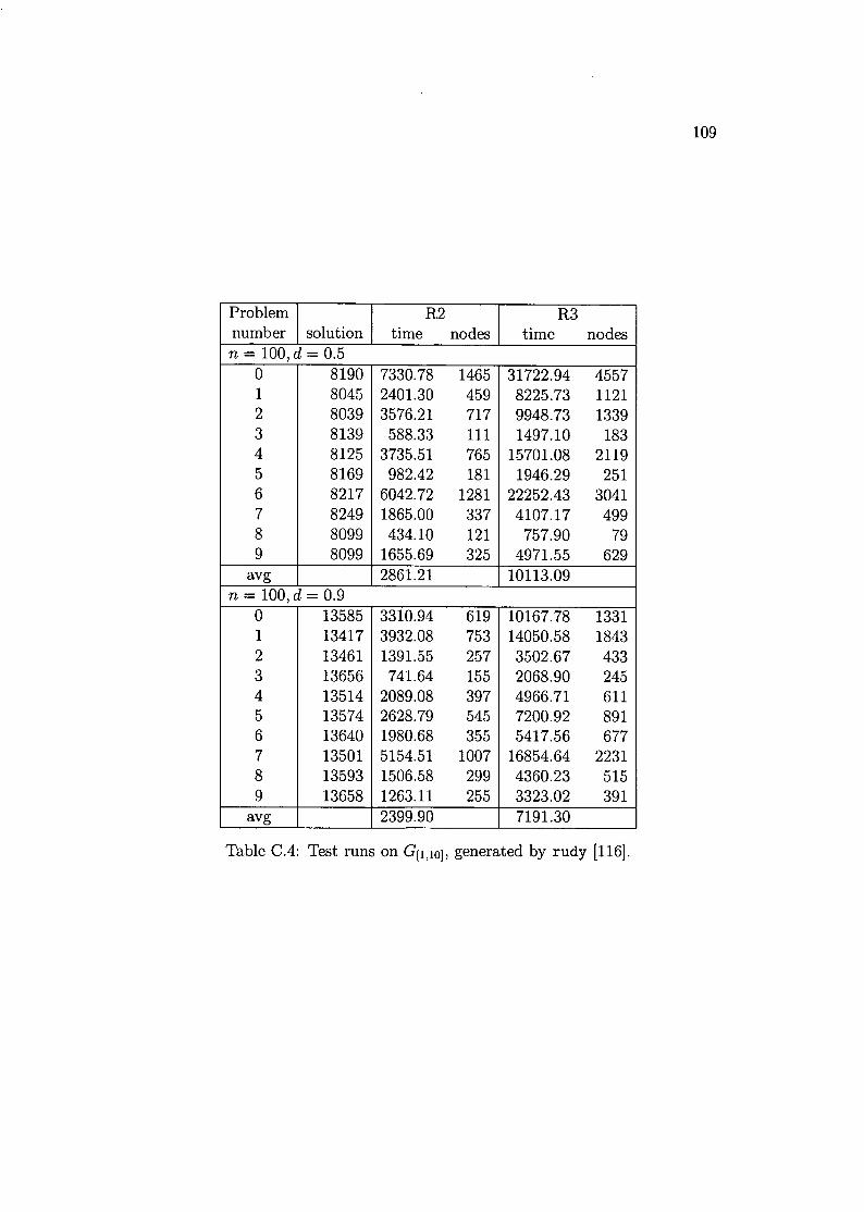
Problem R2 R3number solution time nodes time nodesn = 100,d = 0.5
0 8190 7330.78 1465 31722.94 45571 8045 2401.30 459 8225.73 11212 8039 3576.21 717 9948.73 13393 8139 588.33 111 1497.10 1834 8125 3735.51 765 15701.08 21195 8169 982.42 181 1946.29 2516 8217 6042.72 1281 22252.43 30417 8249 1865.00 337 4107.17 4998 8099 434.10 121 757.90 799 8099 1655.69 325 4971.55 629
avg 2861.21 10113.09n = 100, d = 0.9
0 13585 3310.94 619 10167.78 13311 13417 3932.08 753 14050.58 18432 13461 1391.55 257 3502.67 4333 13656 741.64 155 2068.90 2454 13514 2089.08 397 4966.71 6115 13574 2628.79 545 7200.92 8916 13640 1980.68 355 5417.56 6777 13501 5154.51 1007 16854.64 22318 13593 1506.58 299 4360.23 5159 13658 1263.11 255 3323.02 391
avg 2399.90 7191.30
Table C.4: Test runs on C[I,lOl, generated by rudy [116].
109
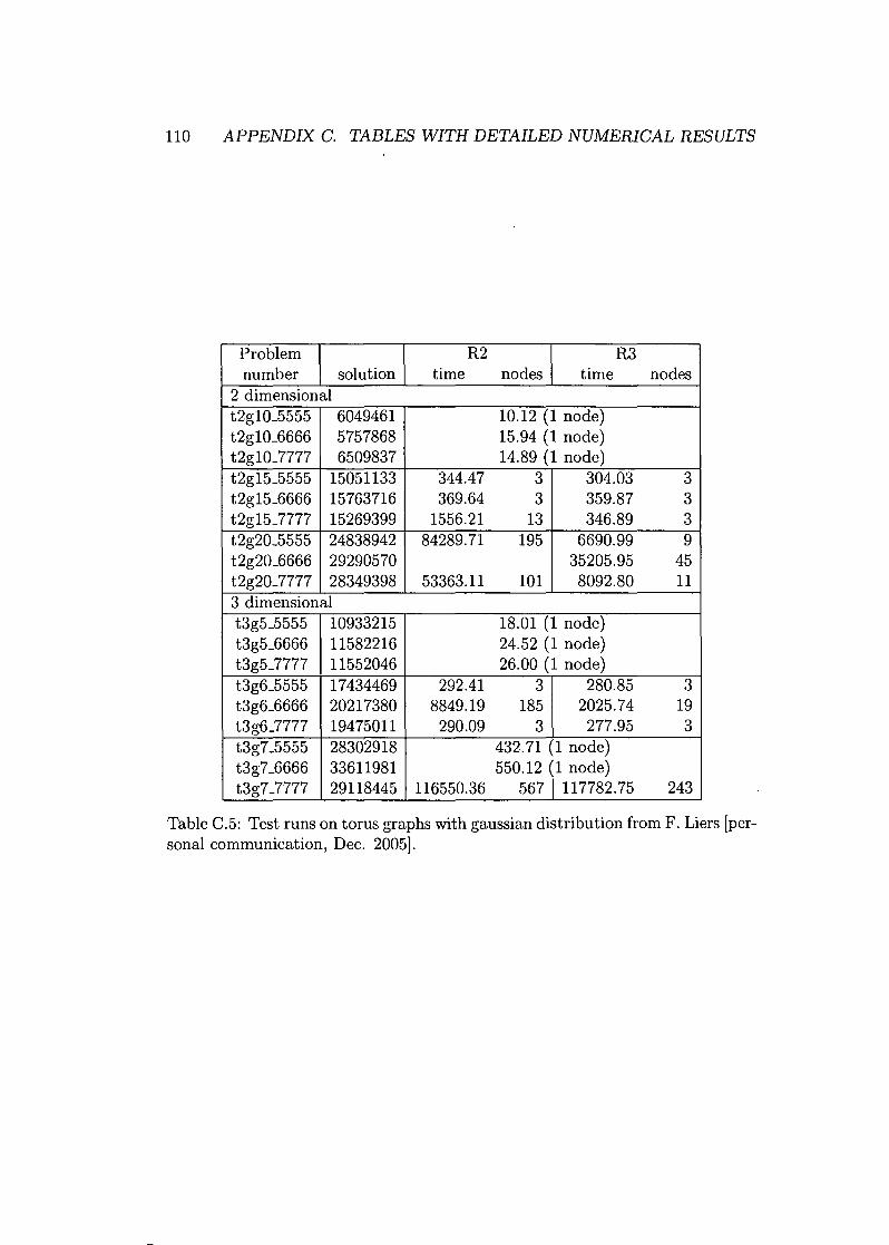
110 APPENDIX C. TABLES WITH DETAILED NUMERICAL RESULTS
Problem R2 R3number solution time nodes time nodes
2 dimensionalt2g10_5555 6049461 10.12 (1 node)t2g10_6666 5757868 15.94 (1 node)t2g103777 6509837 14.89 (1 node)t2g15_5555 15051133 344.47 3 304.03 3t2g15_6666 15763716 369.64 3 359.87 3t2g153777 15269399 1556.21 13 346.89 3t2g20_5555 24838942 84289.71 195 6690.99 9t2g20_6666 29290570 35205.95 45t2g203777 28349398 53363.11 101 8092.80 113 dimensionalt3g5_5555 10933215 18.01 (1 node)t3g5_6666 11582216 24.52 (1 node)t3g53777 11552046 26.00 (1 node)t3g6_5555 17434469 292.41 3 280.85 3t3g6_6666 20217380 8849.19 185 2025.74 19t3g63777 19475011 290.09 3 277.95 3t3g7_5555 28302918 432.71 (1 node)t3g7_6666 33611981 550.12 (1 node)t3g73777 29118445 116550.36 567 1117782.75 243
Table C.5: Test runs on torus graphs with gaussian distribution from F. Liers [per-sonal communication, Dec. 2005].

111
Problem R2 R3number solution time nodes time nodes
n = 1002.5-100_5555 2460049 542.28 85 92.43 72.5-100_6666 2031217 502.50 55 65.65 52.5-100-7777 3363230 654.60 81 47.49 33.0-100_5555 2448189 276.21 91 96.45 73.0-100_6666 1984099 306.41 137 33.82 33.0-100-7777 3335814 80.70 5 48.16 3n = 1502.5-150_5555 4363532 1342.15 49 265.14 72.5-150_6666 4057153 2940.15 167 338.94 72.5-150-7777 4243269 2752.18 157 559.14 113.0-150_5555 4279261 1932.23 157 278.02 73.0-150_6666 3949317 1229.10 127 235.00 73.0-150-7777 4211158 1852.36 147 366.80 9n = 2002.5-200_5555 6294701 8139.05 277 604.76 72.5-200_6666 6795365 4518.01 73 1074.65 112.5-200-7777 5568272 10258.25 599 1298.48 133.0-200_5555 6215531 7048.29 263 607.20 93.0-200_6666 6756263 4806.96 115 1133.12 133.0-200-7777 5560824 8357.32 557 1362.60 15n = 2502.5-250_5555 7919449 14740.00 409 10828.49 592.5-250_6666 6925717 7581.61 87 4623.67 272.5-250-7777 6596797 15868.20 739 4249.66 233.0-250_5555 7823791* 16351.90 739 6388.59 393.0-250_6666 6903351* 16529.27 526 949.19 53.0-250-7777 6418276* 11979.72 251 3443.85 19n = 3002.5-300_5555 8579363 77388.27 1207 24226.96 832.5-300_6666 9102033 79469.93 1041 32678.08 1052.5-300-7777 8323804 102622.88 1523 46810.17 1393.0-300_5555 8493173* 26310.19 499 8414.36 293.0-300_6666 8915110* 26437.34 169 5541.51 193.0-300-7777 8242904* 29937.24 475 11533.05 39
Table C.6: Test runs on Ising instances from F. Liers [personal communication,Dec. 2005].
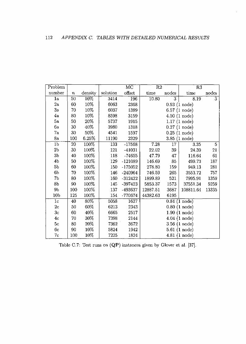
112 APPENDIX C. TABLES WITH DETAILED NUMERICAL RESULTS
Problem MC R2 R3number n density solution offset time nodes time nodes
la 50 10% 3414 196 10.80 3 8.19 32a 60 10% 6063 2368 0.93 (1 node)3a 70 10% 6037 1389 6.57 (1 node)4a 80 10% 8598 3159 4.50 (1 node)5a 50 20% 5737 1915 1.17 (1 node)6a 30 40% 3980 1318 0.27 (1 node)7a 30 50% 4541 1597 0.25 (1 node)8a 100 6.25% 11190 2329 3.85 (1 node)Ib 20 100% 133 -17568 7.28 17 3.35 52b 30 100% 121 -41031 22.02 39 24.30 213b 40 100% 118 -74655 47.79 47 116.64 614b 50 100% 129 -121089 146.69 85 499.73 1875b 60 100% 150 -175052 278.80 159 949.13 2816b 70 100% 146 -240964 746.59 265 3553.72 7577b 80 100% 160 -312422 1899.89 521 7995.91 13598b 90 100% 145 -397423 5853.37 1573 37551.34 52599b 100 100% 137 -493637 12887.51 3687 108811.64 13335lOb 125 100% 154 -770674 44382.63 6195le 40 80% 5058 1627 0.84 (1 node)2c 50 60% 6213 2343 0.80 (1 node)3c 60 40% 6665 2517 1.90 (1 node)4c 70 30% 7398 2144 4.04 (1 node)5c 80 20% 7362 3672 3.56 (1 node)6c 90 10% 5824 1942 5.61 (1 node)7c 100 10% 7225 1824 4.81 (1 node)
Table C.7: Test runs on (QP) instances given by Glover et al. [37].
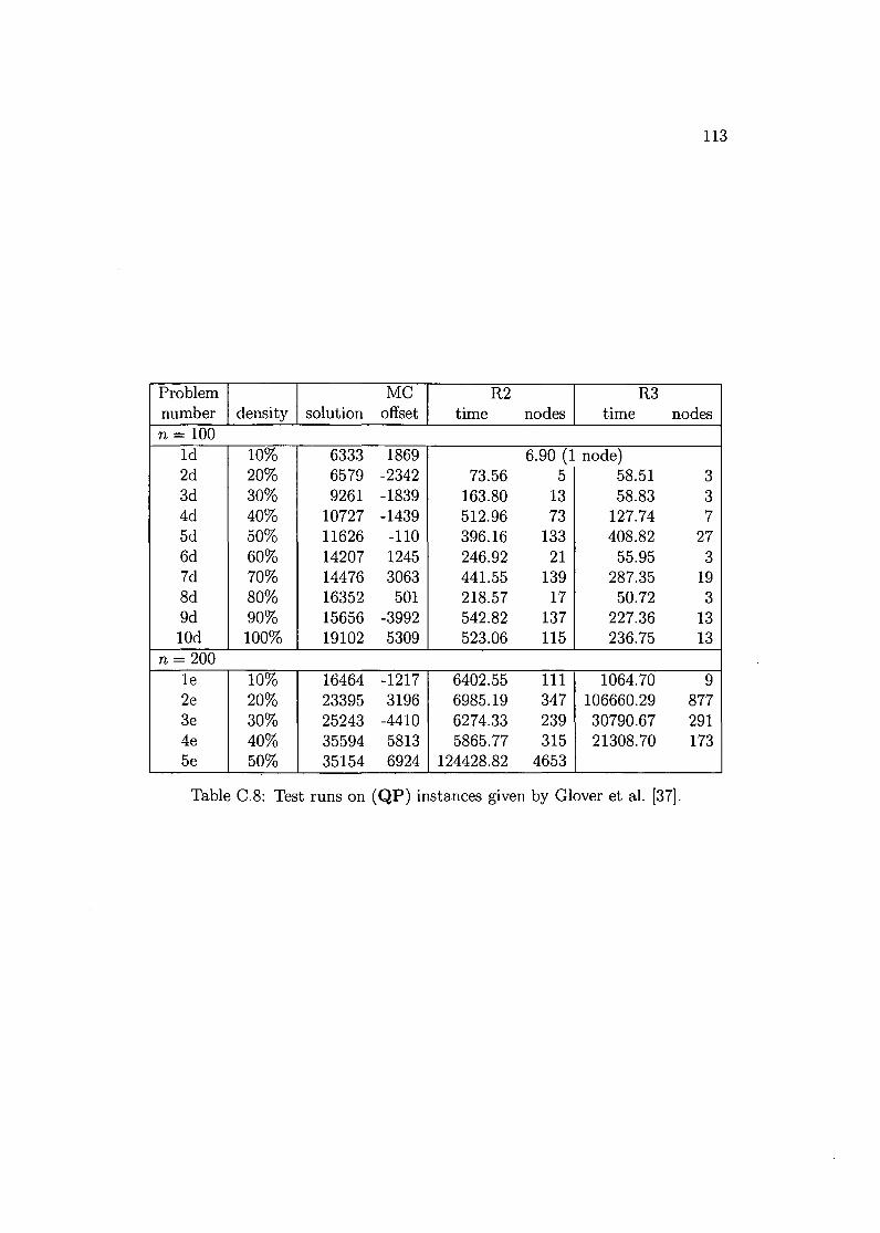
113
Problem MC R2 R3number density solution offset time nodes time nodesn = 100
Id 10% 6333 1869 6.90 (1 node)2d 20% 6579 -2342 73.56 5 58.51 33d 30% 9261 -1839 163.80 13 58.83 34d 40% 10727 -1439 512.96 73 127.74 75d 50% 11626 -110 396.16 133 408.82 276d 60% 14207 1245 246.92 21 55.95 37d 70% 14476 3063 441.55 139 287.35 198d 80% 16352 501 218.57 17 50.72 39d 90% 15656 -3992 542.82 137 227.36 13IOd 100% 19102 5309 523.06 115 236.75 13
n = 200le 10% 16464 -1217 6402.55 111 1064.70 92e 20% 23395 3196 6985.19 347 106660.29 8773e 30% 25243 -4410 6274.33 239 30790.67 2914e 40% 35594 5813 5865.77 315 21308.70 1735e 50% 35154 6924 124428.82 4653
Table C.8: Test runs on (QP) instances given by Glover et al. [37].
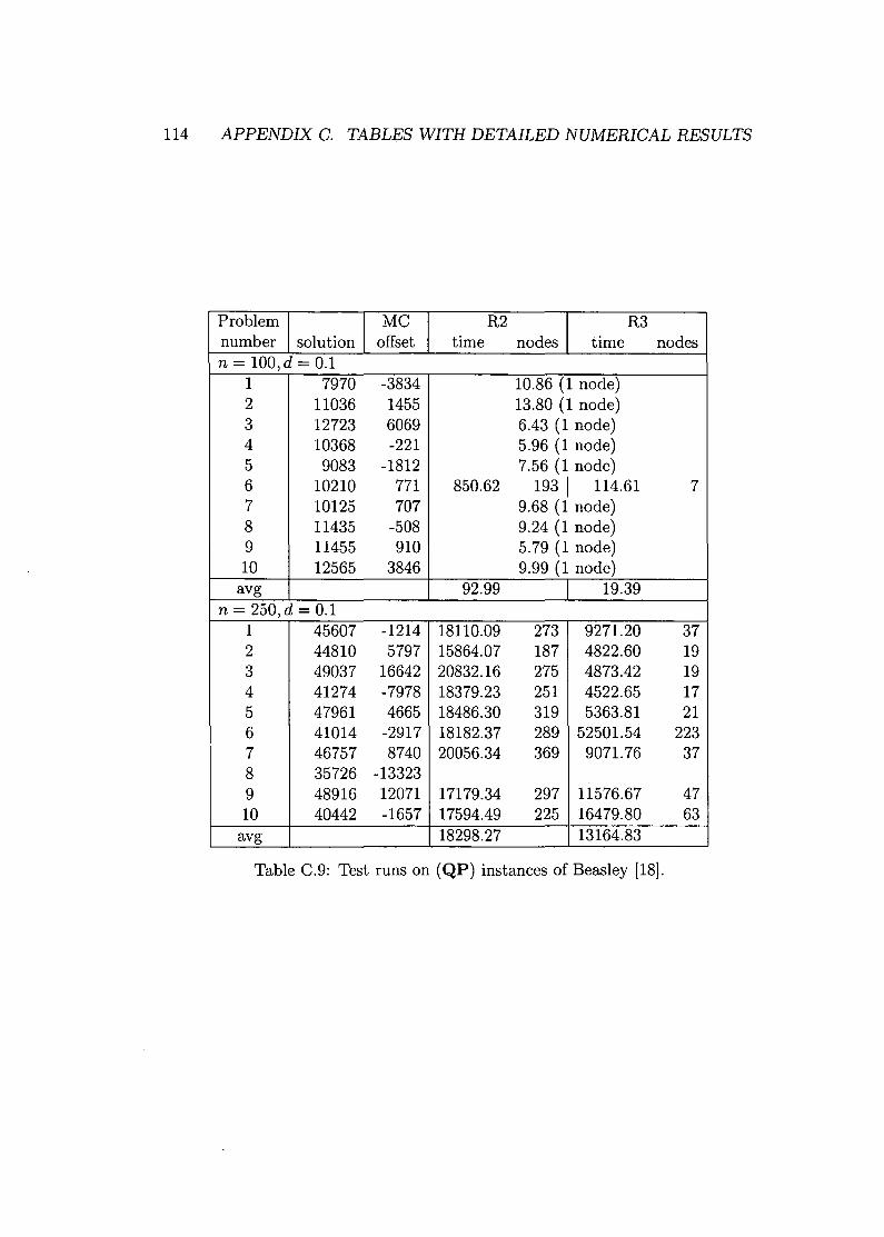
114 APPENDIX C. TABLES WITH DETAILED NUMERICAL RESULTS
Problem I MC R2 R3number solution offset time nodes time nodesn = 100,d = 0.1
1 7970 -3834 10.86 (1 node)2 11036 1455 13.80 (1 node)3 12723 6069 6.43 (1 node)4 10368 -221 5.96 (1 node)5 9083 -1812 7.56 (1 node)6 10210 771 850.62 193 I 114.61 77 10125 707 9.68 (1 node)8 11435 -508 9.24 (1 node)9 11455 910 5.79 (1 node)10 12565 3846 9.99 (1 node)avg 92.99 19.39
n = 250, d = 0.11 45607 -1214 18110.09 273 9271.20 372 44810 5797 15864.07 187 4822.60 193 49037 16642 20832.16 275 4873.42 194 41274 -7978 18379.23 251 4522.65 175 47961 4665 18486.30 319 5363.81 216 41014 -2917 18182.37 289 52501.54 2237 46757 8740 20056.34 369 9071.76 378 35726 -133239 48916 12071 17179.34 297 11576.67 4710 40442 -1657 17594.49 225 16479.80 63avg 18298.27 13164.83
Table C.9: Test runs on (QP) instances of Beasley [18].
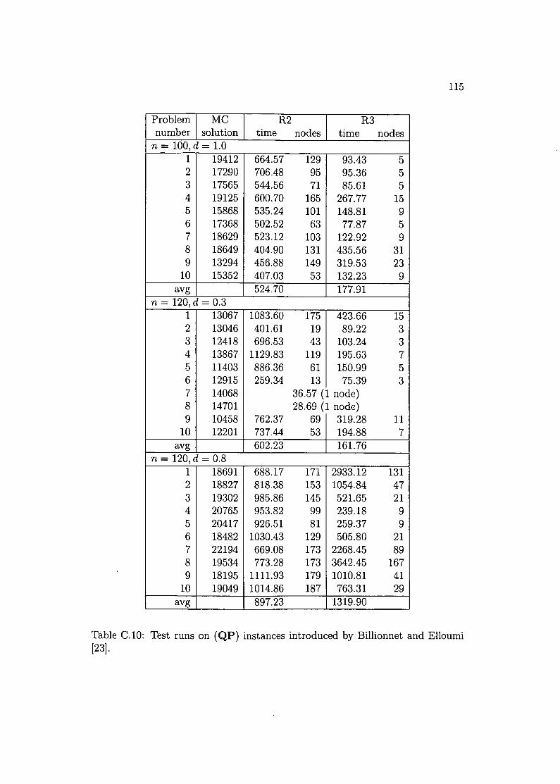
115
Problem MC R2 R3number solution time nodes time nodesn = 100, d = 1.0
1 19412 664.57 129 93.43 52 17290 706.48 95 95.36 53 17565 544.56 71 85.61 54 19125 600.70 165 267.77 155 15868 535.24 101 148.81 96 17368 502.52 63 77.87 57 18629 523.12 103 122.92 98 18649 404.90 131 435.56 319 13294 456.88 149 319.53 23
10 15352 407.03 53 132.23 9avg 524.70 177.91
n = 120, d = 0.31 13067 1083.60 175 423.66 152 13046 401.61 19 89.22 33 12418 696.53 43 103.24 34 13867 1129.83 119 195.63 75 11403 886.36 61 150.99 56 12915 259.34 13 75.39 37 14068 36.57 (1 node)8 14701 28.69 (1 node)9 10458 762.37 69 319.28 11
10 12201 737.44 53 194.88 7avg 602.23 161.76
n = 120, d = 0.81 18691 688.17 171 2933.12 1312 18827 818.38 153 1054.84 473 19302 985.86 145 521.65 214 20765 953.82 99 239.18 95 20417 926.51 81 259.37 96 18482 1030.43 129 505.80 217 22194 669.08 173 2268.45 898 19534 773.28 173 3642.45 1679 18195 1111.93 179 1010.81 41
10 19049 1014.86 187 763.31 29avg 897.23 1319.90
Table C.10: Test runs on (QP) instances introduced by Billionnet and Elloumi[23].
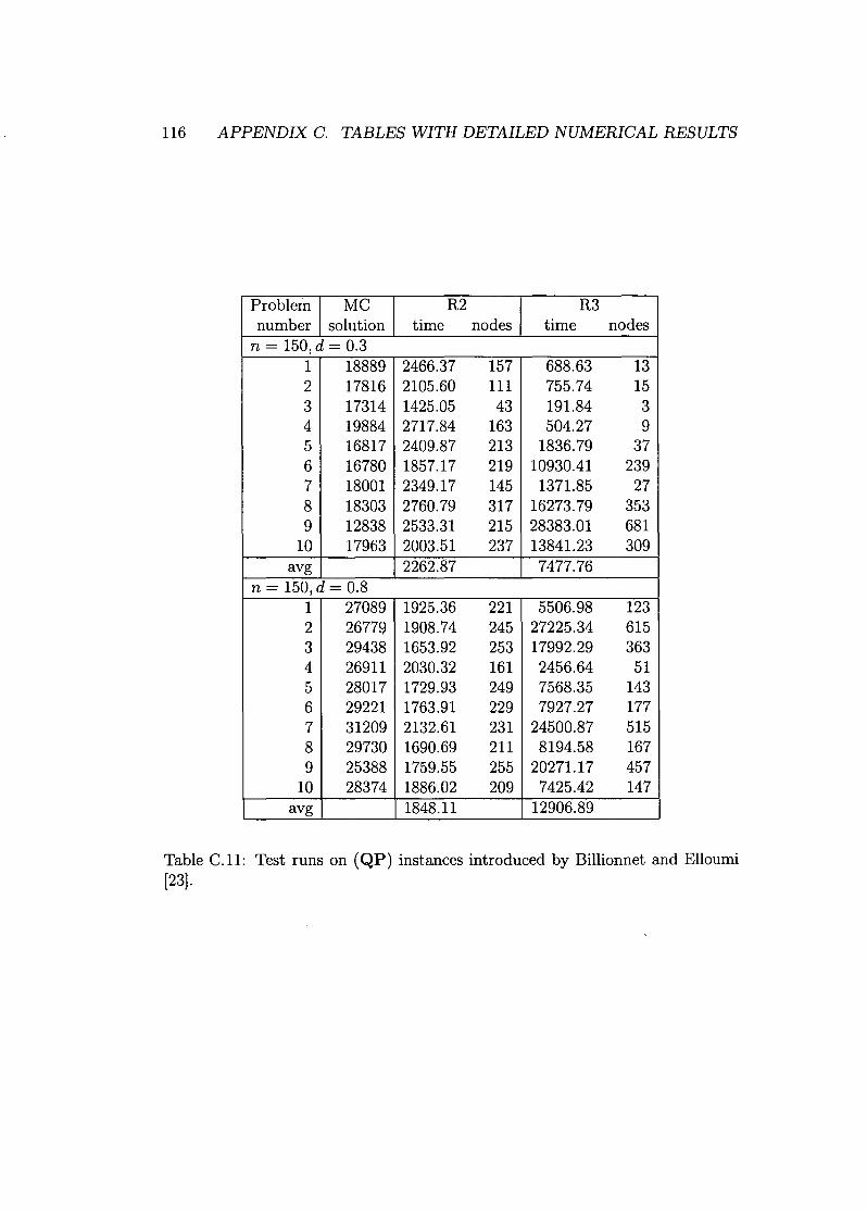
116 APPENDIX C. TABLES WITH DETAILED NUMERICAL RESULTS
Problem MC R2 R3number solution time nodes time nodes
n = 150,d = 0.31 18889 2466.37 157 688.63 132 17816 2105.60 111 755.74 153 17314 1425.05 43 191.84 34 19884 2717.84 163 504.27 95 16817 2409.87 213 1836.79 376 16780 1857.17 219 10930.41 2397 18001 2349.17 145 1371.85 278 18303 2760.79 317 16273.79 3539 12838 2533.31 215 28383.01 681
10 17963 2003.51 237 13841.23 309avg 2262.87 7477.76
n = 150, d = 0.81 27089 1925.36 221 5506.98 1232 26779 1908.74 245 27225.34 6153 29438 1653.92 253 17992.29 3634 26911 2030.32 161 2456.64 515 28017 1729.93 249 7568.35 1436 29221 1763.91 229 7927.27 1777 31209 2132.61 231 24500.87 5158 29730 1690.69 211 8194.58 1679 25388 1759.55 255 20271.17 457
10 28374 1886.02 209 7425.42 147avg 1848.11 12906.89
Table C.11: Test runs on (QP) instances introduced by Billionnet and Elloumi[23].
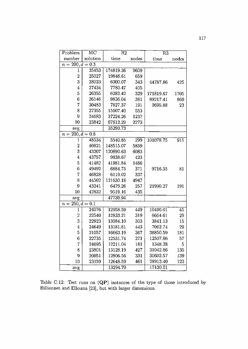
117
Problem MC R2 R3number solution time nodes time nodes
n = 200, d = 0.31 25453 174819.36 96092 25027 19846.61 6593 28023 6300.07 343 44787.86 4254 27434 7780.47 4055 26355 6282.42 329 171819.67 17056 26146 9836.04 381 89217.41 8697 30483 7627.37 191 2695.88 238 27355 15607.40 5539 24683 37224.26 1237
10 23842 67613.29 2273avg 35293.73
n = 200, d = 0.81 48534 5540.85 299 101078.75 9112 40821 148515.07 58593 43207 120890.63 60834 43757 9838.67 4235 41482 41981.84 14866 49492 6884.75 371 9716.35 817 46828 6119.02 3378 44502 121630.18 49479 43241 6479.26 257 21990.27 191
10 42832 9519.16 435avg 47739.94
n = 250, d = 0.11 24076 12958.59 449 10466.01 452 22540 12833.21 319 6664.61 293 22923 13984.10 303 3841.13 154 24649 13181.81 443 7062.74 295 21057 16663.19 367 38850.59 1816 22735 12531.74 271 12507.86 577 24095 12211.04 181 1348.28 58 23801 13128.19 427 31042.86 1359 20051 12806.56 331 30602.57 139
10 23159 12648.59 461 28913.40 123avg 13294.70 17130.01
Table C.12: Test runs on (QP) instances of the type of those introduced byBillionnet and Elloumi [23], but with larger dimensions.

118 APPENDIX C. TABLES WITH DETAILED NUMERICAL RESULTS
Bibliography
[1] Farid Alizadeh. Interior point methods in semidefinite programming withapplications to combinatorial optimization. SIAM J. Optim., 5(1):13-51,1995.
[2] Noga Alon and Nabil Kahale. Approximating the independence numbervia the O-function. Math. Programming, 80(3, Ser. A):253-264, 1998.
[3] Miguel F. Anjos and Henry Wolkowicz. Strengthened semidefinite relax-ations via a second lifting for the Max-Cut problem. Discrete Appl. Math.,119(1-2):79-106,2002.
[4] Michael Armbruster, Michael L. Overton, Franz Rendl, and AngelikaWiegele. The spectral bundle method with second order information. Tech-nical report, Alpen-Adria-Universität Klagenfurt, Universitätsstr. 65-67,9020 Klagenfurt, Austria, 2005.
[5] W. E. Arnoldi. The principle of minimized iteration in the solution of thematrix eigenvalue problem. Quart. Appl. Math., 9:17-29, 1951.
[6] Sanjeev Arora, Carsten Lund, Rajeev Motwani, Madhu Sudan, and MarioSzegedy. Proof verification and the hardness of approximation problems.J. ACM, 45(3):501-555, 1998.
[7] Laura Bahiense, Nelson F. Maculan, and Claudia A. Sagastizabal. Thevolume algorithm revisited: relation with bundle methods. Math. Program.,94(1, SeroA):41-69, 2002.
[8] Egon Balas, Sebastian Ceria, and Gérard Cornuéjols. A lift-and-projectcutting plane algorithm for mixed 0-1 programs. Math. Programming, 58(3, Ser. A):295-324, 1993.
[9] Francisco Barahona. The max-cut problem on graphs not contractible toKs. Oper. Res. Lett., 2(3):107-111, 1983.
[10] Francisco Barahona. On cuts and matchings in planar graphs. Math. Pro-gramming, 60(1, Ser. A):53-68, 1993.
119
120 BIBLIOGRAPHY
[11] Francisco Barahona and Ranga Anbil. The volume algorithm: producingprimal solutions with a subgradient method. Math. Program., 87(3, Ser.A):385-399, 2000.
[12] Francisco Barahona and Laszl6 Ladanyi. Branch and cut based on thevolume algorithm: Steiner trees in graphs and max-cut. RAIRa Oper.Res., 40(1):53-73, 2006.
[13] Francisco Barahona and Ali Ridha Mahjoub. On the cut polytope. Math.Programming, 36(2): 157-173, 1986.
[14] Francisco Barahona, Michael Jünger, and Gerhard Reinelt. Experiments inquadratic 0-1 programming. Math. Programming, 44(2, (Ser. A)):127-137,1989.
[15] Earl R Barnes and Alan J. Hoffman. Partitioning, spectra and linearprogramming. In Progress in combinatorial optimization (Waterloo, ant.,1982), pages 13-25. Academic Press, Toronto, ON, 1984.
[16] John E. Beasley. Or-library: distributing test problems by electronic mail.J. Oper. Res. Soc., 41(11):1069-1072, 1990.
[17] John E. Beasley. Or-library. http://people .brunel. ac. uk/~mastjjb/j eb/info. html.
[18] John E. Beasley. Heuristic algorithms for the unconstrained binaryquadratic programming problem. Technical report, The ManagementSchool, Imperial College, London SW7 2AZ, England, 1998.
[19] Richard Bellman and Ky Fan. On systems of linear inequalities in Hermitianmatrix variables. In Proc. Sympos. Pure Math., Vol. VII, pages 1-11. Amer.Math. Soc., Providence, RI., 1963.
[20] Claude Berge. Perfect graphs. In Six papers on Graph Theory, pages 1-21.Academic Press, Indian Statistical Institute, Calcutta, 1963.
[21] Claude Berge. Un application de la theorie des graphes à un problemede codage. ln E. R Caianiello, editor, Automata Theory, pages 25-34.Academic Press, 1966.
[22] Dimitri P. Bertsekas. Constrained optimization and Lagrange multipliermethods. Computer Science and Applied Mathematics. Academic PressInc. [Harcourt Brace Jovanovich Publishers], New York, 1982.
[23] Alain Billionnet and Sourour Elloumi. Using a mixed integer quadraticprogramming solver for the unconstrained quadratic 0-1 problem. Math.Programming, 2006. to appear.
BIBLIOGRAPHY 121
[24] Brian Borchers. CSDP, a C library for semidefinite programming. Optim.Methods Softw., 11/12(1-4):613-623, 1999.
[25] Endre Boros, Peter L. Hammer, and Gabriel Tavares. The pseudo-booleanoptimization website, 2005. http://rutcor .rutgers. edu/~pbo/.
[26] Samuel Burer and Renato D. C. Monteiro. A nonlinear programming algo-rithm for solving semidefinite programs via low-rank factorization. Math.Program., 95(2, Ser. B):329-357, 2003.
[27] Samuel Burer and Dieter Vandenbussche. Solving lift-and-project relax-ations of binary integer programs. SIAM J. Optim., 16(3):726-750 (elec-tronic), 2006.
[28] Maria Chudnovsky, Neil Robertson, P. D. Seymour, and Robin Thomas.Progress on perfect graphs. Math. Program., 97(1-2, Sero B):405-422, 2003.
[29] Etienne de Klerk. Aspects of semidefinite programming, volume 65 of Ap-plied Optimization. Kluwer Academic Publishers, Dordrecht, 2002.
[30] Charles Delorme and Svatopluk Poljak. Laplacian eigenvalues and the max-imum cut problem. Math. Programming, 62(3, Ser. A):557-574, 1993.
[31] Michel Deza and Monique Laurent. Applications of cut polyhedra. I, II. J.Comput. Appl. Math., 55(2):191-216, 217-247, 1994.
[32] Michel Marie Deza and Monique Laurent. Geometry of cuts and metrics,volume 15 of Algorithms and Combinatorics. Springer-Verlag, Berlin, 1997.
[33] Wilm E. Donath and Alan J. Hoffman. Lower bounds for the partitioningof graphs. IBM J. Res. Develop., 17:420-425, 1973.
[34] Richard J. Duffin. Infinite programs. In Linear inequalities and relatedsystems, Annals of Mathematics Studies, no. 38, pages 157-170. PrincetonUniversity Press, Princeton, N. J., 1956.
[35] Ilse Fischer, Gerald Gruber, Franz Rendl, and Renata Sotirov. Compu-tational experience with a bundle approach for semidefinite cutting planerelaxations of Max-Cut and equipartition. Math. Program., 105(2-3, Ser.B):451-469,2006.
[36] Michael R. Garey and David S. Johnson. Computers and intractability. W.H. Freeman and Co., San Francisco, Calif., 1979.
[37] Fred Glover, Gary Kochenberger, and Bahram Alidaee. Adaptative memorytabu search for binary quadratic programs. Management Sei., 44(3):336-345, 1998.
122 BIBLIOGRAPHY
[38] Michel X. Goemans and David P. Williamson. New ~-approximation algo-rithms for the maximum satisfiability problem. SIAM J. Discrete Math., 7(4):656-666, 1994.
[39] Michel X. Goemans and David P. Williamson. Improved approximationalgorithms for maximum cut and satisfiability problems using semidefiniteprogramming. J. Assoc. Gomput. Mach., 42(6):1115-1145, 1995.
[40] Édouard Goursat. Functions of a complex variable, 2, Pt. 1. Ginn & Co.,1916.
[41] Martin Grätschel and George L. Nemhauser. A polynomial algorithm forthe max-cut problem on graphs without long odd cycles. Math. Program-ming, 29(1):28-40, 1984.
[42] Martin Grätschei, Laszl6 Lovasz, and Alexander Schrijver. The ellipsoidmethod and its consequences in combinatorial optimization. Gombinator-ica, 1(2):169-197, 1981.
[43] Martin Grätschei, Laszl6 Lovasz, and Alexander Schrijver. Geometric algo-rithms and combinatorial optimization, volume 2 of Algorithms and Gom-binatorics: Study and Research Texts. Springer-Verlag, Berlin, 1988.
[44] Nebojsa Gvozdenovié and Monique Laurent. Approximating the chromaticnumber of a graph by semidefinite programming. Technical report, Centrumvoor Wiskunde en Informatica, Kruislaan 413, 1098 SJ Amsterdam, TheNetherlands, 2006.
[45] Frank O. Hadlock. Finding a maximum cut of a planar graph in polynomialtime. SIAM J. Gomput., 4(3):221-225, 1975.
[46] Peter 1. Hammer. Some network flow problems solved with pseudo-Booleanprogramming. Operations Res., 13:388-399, 1965.
[47] Pierre Hansen. Methods of nonlinear 0 - 1 programming. Ann. DiscreteMath., 5:53-70, 1979.
[48] Johan Hästad. Some optimal inapproximability results. In STOG '97 (ElPaso, TX), pages 1-10 (electronic). ACM, New York, 1999.
[49] Christoph Helmberg. Semidefinite programming website. http: / /www-user.tu-chemnitz.de/~helmberg/semidef.html.
[50] Christoph Helmberg. Fixing variables in semidefinite relaxations. SIAM J.Matrix Anal. Appl., 21(3):952-969 (electronic), 2000.
BIBLIOGRAPHY 123
[51] Christoph Helmberg. Semidefinite programming for combinatorial opti-mization, 2000. Habilitation thesis.
[52] Christoph Helmberg. Semidefinite programming. European J. Oper. Res.,137(3):461-482, 2002.
[53] Christoph Helmberg and Francois Oustry. Bundle methods to minimize themaximum eigenvalue function. In Handbook of semidefinite programming,volume 27 of Internat. Sero Oper. Res. Management Sei., pages 307-337.Kluwer Acad. Pub!., Boston, MA, 2000.
[54] Christoph Helmberg and Franz Rend!. Solving quadratic (0, I)-problemsby semidefinite programs and cutting planes. Math. Programming, 82(3,Ser. A):291-315, 1998.
[55] Christoph Helmberg and Franz Rend!. A spectral bundle method forsemidefinite programming. SIAM J. Optim., 10(3):673-696 (electronic),2000.
[56] Christoph Helmberg, Franz Rendl, Robert J. Vanderbei, and HenryWolkowicz. An interior-point method for semidefinite programming. SIAMJ. Optim., 6(2):342-361, 1996.
[57] Christoph Helmberg, Krzysztof C. KiwieI, and Franz Rend!. Incorporatinginequality constraints in the spectral bundle method. In Integer program-ming and combinatorial optimization (Houston, TX, 1998), volume 1412 ofLecture Notes in Comput. Sei., pages 423-435. Springer, Berlin, 1998.
[58] Nicholas J. Higham. Computing a nearest symmetric positive semidefinitematrix. Linear Algebra Appl., 103:103-118, 1988.
[59] Jean-Baptiste Hiriart-Urruty and Claude Lemarécha!. Convex analysis andminimization algorithms. I, volume 305 of Grundlehren der Mathematis-chen Wissenschaften [Fundamental Principles of Mathematical Sciences].Springer-Verlag, Berlin, 1993.
[60] Jean-Baptiste Hiriart-Urruty and Claude Lemarécha!. Convex analysis andminimization algorithms. II, volume 306 of Grundlehren der Mathematis-chen Wissenschaften [Fundamental Principles of Mathematical Sciences].Springer-Verlag, Berlin, 1993.
[61] Roger A. Horn and Charles R. Johnson. Matrix analysis. Cambridge Uni-versity Press, Cambridge, 1985.
[62] David S. Johnson. Approximation algorithms for combinatorial problems.J. Comput. System Sei., 9:256-278, 1974.
124 BIBLIOGRAPHY
[63] David S. Johnson, Cecilia R. Aragon, Lyle A. McGeoch, and CatherineSchevon. Optimization by simulated annealing: an experimental evaluation.part i, graph partitioning. Oper. Res., 37(6):865-892, 1989.
[64] David Karger, Rajeev Motwani, and Madhu Sudan. Approximate graphcoloring by semidefinite programming. J. ACM, 45(2):246-265, 1998.
[65] Stefan E. Karisch and Franz Rendl. Semidefinite programming andgraph equipartition. In Topics in semidefinite and interior-point methods(Toronto, ON, 1996), volume 18 of Fields Inst. Commun., pages 77-95.Amer. Math. Soc., Providence, RI, 1998.
[66] Richard M. Karp. Reducibility among combinatorial problems. In Com-plexity of computer computations (Proc. Sympos., IBM Thomas J. WatsonRes. Center, Yorktown Heights, N. Y, 1972), pages 85-103. Plenum, NewYork,1972.
[67] Hans Kellerer, Ulrich Pferschy, and David Pisinger. Knapsack problems.Springer-Verlag, Berlin, 2004.
[68] Sunyoung Kim and Masakazu Kojima. Second order cone programmingrelaxation of nonconvex quadratic optimization problems. Optim. MethodsSoftw., 15(3-4):201-224,2001.
[69] Krzysztof C. Kiwiel. Methods of descent for nondifferentiable optimization,volume 1133 of Lecture Notes in Mathematics. Springer- Verlag, Berlin,1985.
[70] Krzysztof C. Kiwiel. A survey of bundle methods for nondifferentiableoptimization. In Mathematical programming (Tokyo, 1988), volume 6 ofMath. Appt. (Japanese Ser.), pages 263-282. SCIPRESS, Tokyo, 1989.
[71] Krzysztof C. Kiwiel. Proximity control in bundle methods for convex non-differentiable minimization. Math. Programming, 46(1, (Ser. A)):105-122,1990.
[72] Donald E. Knuth. The sandwich theorem. Electron. J. Combin., I:Article1, approx. 48 pp. (electronic), 1994.
[73] Michal Kocvara and Michael Stingl. On the solution of large-scale SDPproblems by the modified barrier method using iterative solvers. Math.Programming. Published online: September 2006.
[74] Masakazu Kojima, Susumu Shindoh, and Shinji Hara. Interior-point meth-ods for the monotone semidefinite linear complementarity problem in sym-metric matrices. SIAM J. Optim., 7(1):86-125, 1997.
BIBLIOGRAPHY 125
[75] Peter Lancaster. On eigenvalues of matrices dependent on a parameter.Numer. Math., 6:377-387, 1964.
[76] Jean B. Lasserre. An explicit equivalent positive semidefinite program fornonlinear 0-1 programs. SIAM J. Optim., 12(3):756-769 (electronic), 2002.
[77] Monique Laurent. A comparison of the Sherali-Adams, Lovasz-Schrijver,and Lasserre relaxations for 0-1 programming. Math. Oper. Res., 28(3):470-496, 2003.
[78] Monique Laurent and Svatopluk Poljak. On a positive semidefinite relax-ation of the cut polytope. Linear Algebra Appl., 223/224:439-461, 1995.
[79] Monique Laurent and Svatopluk Poljak. On the facial structure of the setof correlation matrices. SIAM J. Matrix Anal. Appl., 17(3):530-547, 1996.
[80] Monique Laurent and Franz Rendl. Semidefinite programming and integerprogramming. In K. Aardal, G.L. Nemhauser, and R. Weismantel, editors,Discrete Optimization, volume 12 of Handbooks in Operations Research andManagement Science, chapter 8, pages 393-514. Elsevier, Amsterdam, TheNetherlands, 2005.
[81] Richard B. Lehoucq, Danny C. Sorensen, and Chao Yang. ARPACK users'guide, volume 6 of Software, Environments, and Tools. Society for Industrialand Applied Mathematics (SIAM), Philadelphia, PA, 1998.
[82] Claude Lemarechal. Bundle methods in nonsmooth optimization. In Non-smooth optimization (Proc. IIASA Workshop, Laxenburg, 1977), volume 3of IIASA Proc. Ser., pages 79-102. Pergamon, Oxford, 1978.
[83] Claude Lemaréchal, Arkadii Nemirovskii, and Yurii Nesterov. New variantsof bundle methods. Math. Programming, 69(1, Ser. B):111-147, 1995.
[84] Thomas Lengauer. Combinatorial algorithms for integrated circuit layout.Applicable Theory in Computer Science. John Wiley & Sons Ltd., Chich-ester, 1990.
[85] Adrian S. Lewis and Michael L. Overton. Eigenvalue optimization. In Actanumerica, 1996, volume 5 of Acta Numer., pages 149-190. Cambridge Univ.Press, Cambridge, 1996.
[86] Frauke Liers. Contributions to Determining Exact Ground-States of IsingSpin-Glasses and to their Physics. PhD thesis, Universität zu Köln, 2004.
[87] Frauke Liers, Michael Jünger, Gerhard Reinelt, and Giovanni Rinaldi. Com-puting Exact Ground States of Hard Ising Spin Glass Problems by Branch-and-Cut, pages 47-68. Wiley, 2004.
126 BIBLIOGRAPHY
[88] Laszlo Lovasz. On the Shannon capacity of a graph. IEEE Trans. Inform.Theory, 25(1):1-7, 1979.
[89] Laszlo Lovasz and Alexander Schrijver. Cones of matrices and set-functionsand 0-1 optimization. SIAM J. Optim., 1(2):166-190, 1991.
[90] Carsten Lund and Mihalis Yannakakis. On the hardness of approximatingminimization problems. J. Assoc. Comput. Mach., 41(5):960-981, 1994.
[91] Marko M. Mäkelä. Survey of bundle methods for nonsmooth optimization.Optim. Methods Softw., 17(1):1-29, 2002.
[92] Jérôme Malick. A dual approach to semidefinite least-squares problems.SIAM J. Matrix Anal. Appl., 26(1):272-284 (electronic), 2004.
[93] Jérôme Malick, Janez Povh, Franz Rendl, and Angelika Wiegele. Proximalmethods for semidefinite programming. Technical report, Alpen-Adria-Universität Klagenfurt, Universitätsstr. 65-67, 9020 Klagenfurt, Austria,2006.
[94] Hans Mittelmann. Benchmarks for optimization software. http://plato .asu.edu/bench.html.
[95] Renato D. C. Monteiro. Primal-dual path-following algorithms for semidef-inite programming. SIAM J. Optim., 7(3):663-678, 1997.
[96] Renato D. C. Monteiro and Michael J. Todd. Path-following methods. InHandbook of semidefinite programming, volume 27 of Internat. Sero Oper.Res. Management Sei., pages 267-306. Kluwer Acad. Pub!., Boston, MA,2000.
[97] Masakazu Muramatsu and Tsunehiro Suzuki. A new second-order coneprogramming relaxation for MAX-CUT problems. J. Oper. Res. Soc. Japan,46(2):164-177,2003.
[98] Yurii Nesterov and Arkadii Nemirovskii. Interior-point polynomial algo-rithms in convex programming, volume 13 of SIAM Studies in AppliedMathematics. Society for Industrial and Applied Mathematics (SIAM),Philadelphia, PA, 1994.
[99] G. 1. Orlova and Va. G. Dorfman. Finding the maximum cut in a graph.Izv. Akad. Nauk SSSR Tehn. Kibernet., (3):155-159, 1972.
[100] Michael L. Overton. Large-scale optimization of eigenvalues. SIAM J.Optim., 2(1):88-120, 1992.
BIBLIOGRAPHY 127
[101] Michael L. Overton and Robert S. Womersley. Second derivatives for op-timizing eigenvalues of symmetric matrices. SIAM J. Matrix Anal. Appl.,16(3):697-718, 1995.
[102] Panos M. Pardalos and Gregory P. Rodgers. Computational aspects of abranch and bound algorithm for quadratic zero-one programming. Com-puting, 45(2):131-144, 1990.
[103] Panos M. Pardalos and Gregory P. Rodgers. Parallel branch and boundalgorithms for quadratic zero-one programs on the hypercube architecture.Ann. Oper. Res., 22(1-4):271-292, 1990.
[104] Beresford N. Parlett. The symmetric eigenvalue problem, volume 20 ofClassics in Applied Mathematics. Society for Industrial and Applied Math-ematics (SIAM), Philadelphia, PA, 1998.
[105] Svatopluk Poljak. Polyhedral and eigenvalue approximations of the max-cut problem. In Sets, graphs and numbers (Budapest, 1991), volume 60 ofColloq. Math. Soc. Janos Bolyai, pages 569-581. North-Holland, Amster-dam,1992.
[106] Svatopluk Poljak and Franz Rend!. Solving the max-cut problem usingeigenvalues. Discrete Appl. Math., 62(1-3):249-278, 1995.
[107] Svatopluk Poljak and Franz Rend!. Nonpolyhedral relaxations of graph-bisection problems. SIAM J. Optim., 5(3):467-487, 1995.
[108] Svatopluk Poljak and Zsolt Tuza. The expected relative error of the poly-hedral approximation of the max-cut problem. Oper. Res. LeU., 16(4):191-198, 1994.
[109] Svatopluk Poljak and Zsolt Tuza. Maximum cuts and large bipartite sub-graphs. In Combinatorial optimization (New Brunswick, NJ, 1992-1993),volume 20 of DIMACS Sero Discrete Math. Theoret. Comput. Sei., pages181-244. Amer. Math. Soc., Providence, RI, 1995.
[110] Janez Povh, Franz Rendl, and Angelika Wiegele. A Boundary Point Methodto solve Semidefinite Programs. Computing, to appear.
[111] Franz Rend!. Semidefinite programming and combinatorial optimization.Appl. Numer. Math., 29(3):255-281, 1999.
[112] Franz Rendl and Renata Sotirov. Bounds for the quadratic assignmentproblem using the bundle method. Math. Programming. Published online:September 2006.

128 BIBLIOGRAPHY
[113] Franz Rendl and Angelika Wiegele. Semidefinite relaxations for sparsemax-cut problems. Technical report, Alpen-Adria-Universität Klagenfurt,Universitätsstr. 65-67, 9020 Klagenfurt, Austria, 2005.
[114] Franz Rendl and Henry Wolkowicz. A projection technique for partitioningthe nodes of a graph. Ann. Oper. Res., 58:155-179, 1995.
[115] Franz Rendl, Giovanni Rinaldi, and Angelika Wiegele. SDP based Branch &Bound for Max-Cut. Technical report, Alpen-Adria-Universität Klagenfurt,Universitätsstr. 65-67, 9020 Klagenfurt, Austria, 2006.
[116] Giovanni Rinaldi. Rudy. http://www-user.tu-chemnitz.de/~helmberg/rudy. tar. gz.
[117] R. Tyrrell Rockafellar. Convex analysis. Princeton Mathematical Series,No. 28. Princeton University Press, Princeton, N.J., 1970.
[118] Helga Schramm and Jochem Zowe.A version ofthe bundle idea for minimiz-ing a nonsmooth function: conceptual idea, convergence analysis, numericalresults. SIAM J. Optim., 2(1):121-152, 1992.
[119] Alexander Schrijver. Combinatorialoptimization. Polyhedra and efficiency.Vol. A,B, C, volume 24 of Algorithms and Combinatorics. Springer-Verlag,Berlin, 2003.
[120] Alexander Schrijver. On the history of combinatorial optimization (till1960). In K. Aardal, G.L. Nemhauser, and R. Weismantel, editors, Dis-crete Optimization, volume 12 of Handbooks in Operations Research andManagement Science, chapter 1, pages 1-68. Elsevier, Amsterdam, TheNetherlands, 2005.
[121] Hanif D. Sherali and Warren P. Adams. A hierarchy ofrelaxations betweenthe continuous and convex hull representations for zero-one programmingproblems. SIAM J. Discrete Math., 3(3):411-430, 1990.
[122] Jas F. Sturm. Using SeDuMi 1.02, a MATLAB toolbox for optimizationover symmetric cones. Optim. Methods Softw.OPTMS, 11-12:625-653, 1999.
[123] Michael J. Todd. A study of search directions in primal-dual interior-pointmethods for semidefinite programming. Optim. Methods Softw., 11/12(1-4):1-46, 1999.
[124] Kim-Chuan Toh. Solving large scale semidefinite programs via an iterativesolver on the augmented systems. SIAM J. Optim., 14(3):670-698 (elec-tronic), 2003.
BIBLIOGRAPHY 129
[125] Kim-Chuan Toh, Michael J. Todd, and Reha H. Tütüncü. SDPT3-a MAT-LAB software package for semidefinite programming, version 1.3. Optim.Methods Softw., 11/12(1-4):545-581, 1999.
[126] Lieven Vandenberghe and Stephen Boyd. Semidefinite programming. SIAMRev., 38(1):49-95, 1996.
[127] Henry Wolkowicz and Qing Zhao. Semidefinite programming relaxationsfor the graph partitioning problem. Discrete Appt. Math., 96/97:461-479,1999.
Index
adjoint operator, 4aggregate subgradient, 14Augmented Lagrangian method, 65
barrierfunction, 11parameter, 11
Biq Mac, 71, 97algorithm, 78library, 80ud, 95
Bisection problem, 20, 92Boundary point method, 64-69, 97Branch & Bound, 71Branching rules, 73
R2,74R3,74strong branching, 74
Bundle method, 13, 50-57, 97
central path, 11, 12clique, 19coloring problem, 19combinatorial optimization, 17complementary slackness, 8constant trace property, 8convex hull, 100convex set, 100cut polytope, 24
duality gap, 5duality theory, 5
eigenvalue optimization, 8Elliptope, 35
feasibility, 5
strict, 5Fejer Theorem, 994-cycle equalities, 42
Goemans- Williamson hyperplane round-ing, 34, 73
Graph partitioning problem, 20
hypermetric inequalities, 36
incidence vector, 24Interior-Point methods, la, 68Ising instances, 83
KKT-conditions, 11
Laplace matrix, 23Lift-and-project methods, 37Linear programming relaxations, 27
Max-Cut problem, 18, 23properties, 23relaxations, 27
Max-Sat problem, 22Max-kSat problem, 22Max-2Sat, 93
maximum clique problem, 19metric polytope, 36minimax inequality, 100MIQP,32
odd cycle inequalities, 27optimality conditions, 8, 11
Penalty parameter, 50primal-dual central path, 12proximal point, 13
quadratic (0-1) program, 25
130
INDEX
Quadratic Assignment Problem, 22Quadratic Knapsack Problem, 95
Schur complement, 100Second-order cone, 33Semidefinite Programming Problem
dual,5in standard form, 4
Slater constraint qualification, 6SOCP,33Spectral bundle method, 13, 69
Second order model, 58-64, 69, 97stable set problem, 19, 94strict feasibility, 5strong duality, 5
'l9-number, 19triangle equalities, 39triangle inequalities, 27
weak duality, 5
131
Recommended