Nonlinear Micromorphic ContinuumMechanics and Finite Strain
Elastoplasticity
by
Richard A. RegueiroAssistant Professor
Department of Civil, Environmental, and Architectural EngineeringUniversity of Colorado at Boulder
1111 Engineering Dr.428 UCB, ECOT 441
Boulder, CO 80309-0428
for
Weapons and Materials Research DirectorateU.S. Army Research Laboratory
Aberdeen Proving Ground, MD 21005
June 11, 2010
Contract No. W911NF-07-D-0001
TCN 10-077
Scientific Services Program
The views, opinions, and/or findings contained in this report are those of the author(s) and should
not be construed as an official Department of the Army position, policy or decision, unless so
designated by other documentation.
1
REPORT DOCUMENTATION PAGE
Form Approved OMB No. 0704-0188
Public reporting burden for this collection of information is estimated to average 1 hour per response, including the time for reviewing instructions, searching data sources, gathering and maintaining the data needed, and completing and reviewing the collection of information. Send comments regarding this burden estimate or any other aspect of this collection of information, including suggestions for reducing this burden to Washington Headquarters Service, Directorate for Information Operations and Reports, 1215 Jefferson Davis Highway, Suite 1204, Arlington, VA 22202-4302, and to the Office of Management and Budget, Paperwork Reduction Project (0704-0188) Washington, DC 20503. PLEASE DO NOT RETURN YOUR FORM TO THE ABOVE ADDRESS. 1. REPORT DATE (DD-MM-YYYY) 11-06-2010
2. REPORT DATE FINAL REPORT
3. DATES COVERED (From - To) 1 Jun 2008 – 31 May 2010
5a. CONTRACT NUMBER Contract W911NF-07-D-0001 5b. GRANT NUMBER
4. TITLE AND SUBTITLE Nonlinear Micromorphic Continuum Mechanics and Finite Strain Elastoplasticity
5c. PROGRAM ELEMENT NUMBER 5d. PROJECT NUMBER 5e. TASK NUMBER
6. AUTHOR(S) Richard A. Regueiro
5f. WORK UNIT NUMBER 7. PERFORMING ORGANIZATION NAME(S) AND ADDRESS(ES) University of Colorado at Boulder 1111 Engineering Dr. Boulder, CO 80309
8. PERFORMING ORGANIZATION REPORT NUMBER Delivery Order 0356
10. SPONSOR/MONITOR'S ACRONYM(S) ARO
9. SPONSORING/MONITORING AGENCY NAME(S) AND ADDRESS(ES) U.S. Army Research Office P.O. Box 12211 Research Triangle Park, NC 27709 11. SPONSORING/MONITORING
AGENCY REPORT NUMBER TCN 08-080
12. DISTRIBUTION AVAILABILITY STATEMENT May not be released by other than sponsoring organization without approval of US Army Research Office.
13. SUPPLEMENTARY NOTES Task was performed under a Scientific Services Agreement issued by Battelle Chapel Hill Operations, 50101 Governors Drive, Suite 110, Chapel Hill, NC 27517 14. ABSTRACT The report presents the detailed formulation of nonlinear micromorphic continuum kinematics and balance equations (balance of mass; micro-inertia; linear, angular, and first moment of momentum; energy; and the Clausius-Duhem inequality). The theory is extended to elastoplasticity assuming a multiplicative decomposition of the deformation gradient and micro-deformation tensor. A general three-level (macro, micro, and micro-gradient) micromorphic finite strain elastoplasticity theory results, with simpler forms presented for linear isotropic elasticity, J2 flow associative plasticity, and non-associative Drucker-Prager pressure-sensitive plasticity. Assuming small elastic deformations for the class of materials of interest, bound particulate materials (ceramics, metal matrix composites, energetic materials, infrastructure materials, and geologic materials), the constitutive equations formulated in the intermediate configuration are mapped to the current configuration, and a new elastic Truesdell objective higher order stress rate is defined. A semi-implicit time integration scheme is presented for the Drucker-Prager model mapped to the current configuration. A strategy to couple the micromorphic continuum finite element implementation to a direct numerical simulation of the grain-scale response of a bound particulate material is outlined that will lead to a concurrent multiscale computational method for simulating dynamic failure in bound particulate materials. 15. SUBJECT TERMS nonlinear micromorphic continuum mechanics; finite strain elastoplasticity; concurrent multiscale computational method; bound particulate materials
16. SECURITY CLASSIFICATION OF: 19a. NAME OF RESPONSIBLE PERSON
a. REPORT
b. ABSTRACT
c. THIS PAGE
17. LIMITATION OF ABSTRACT
18. NUMBER OF PAGES: 104 19b. TELEPONE NUMBER (Include area code)
Standard Form 298 (Rev. 8-98) Prescribed by ANSI-Std Z39-18

Contents
1 Introduction 9
1.1 Description of problem . . . . . . . . . . . . . . . . . . . . . . . . . . . . . . 9
1.2 Proposed Approach . . . . . . . . . . . . . . . . . . . . . . . . . . . . . . . . 12
1.3 Focus of Report . . . . . . . . . . . . . . . . . . . . . . . . . . . . . . . . . . 13
1.4 Notation . . . . . . . . . . . . . . . . . . . . . . . . . . . . . . . . . . . . . . 14
2 Technical Discussion 16
2.1 Statement of Work (SOW) and Specific Tasks . . . . . . . . . . . . . . . . . 16
2.1.1 Specific Tasks . . . . . . . . . . . . . . . . . . . . . . . . . . . . . . . 18
2.2 Nonlinear micromorphic continuum mechanics . . . . . . . . . . . . . . . . . 19
2.2.1 Kinematics . . . . . . . . . . . . . . . . . . . . . . . . . . . . . . . . 19
2.2.2 Micromorphic balance equations and Clausius-Duhem inequality . . . 22
2.3 Finite strain micromorphic elastoplasticity . . . . . . . . . . . . . . . . . . . 35
2.3.1 Kinematics . . . . . . . . . . . . . . . . . . . . . . . . . . . . . . . . 37
2.3.2 Clausius-Duhem inequality in B . . . . . . . . . . . . . . . . . . . . . 40
2.3.3 Constitutive equations . . . . . . . . . . . . . . . . . . . . . . . . . . 49
2.3.4 Numerical time integration . . . . . . . . . . . . . . . . . . . . . . . . 72
3

2.4 Upscaling from grain-scale to micromorphic elastoplasticity . . . . . . . . . . 79
2.5 Coupled formulation . . . . . . . . . . . . . . . . . . . . . . . . . . . . . . . 81
3 Summary 89
3.1 Results . . . . . . . . . . . . . . . . . . . . . . . . . . . . . . . . . . . . . . . 89
3.2 Conclusions . . . . . . . . . . . . . . . . . . . . . . . . . . . . . . . . . . . . 89
3.3 Future Work . . . . . . . . . . . . . . . . . . . . . . . . . . . . . . . . . . . . 90
4 Bibliography 91
A Derivation of F ′ 97
B Another set of elastic deformation measures 99
C Deformation measures 101
D Distribution 103
4

List of Figures
1.1 (a) Microstructure of alumina, composed of grains bound by glassy phase. (b) SiC
reinforced 2080 aluminum metal matrix composite [Chawla et al., 2004]. The 4
black squares are indents to identify the region. (c) Cracking in explosive HMX
grains and at grain-matrix interfaces [Baer et al., 2007]. (d) Cracking in asphalt
pavement. . . . . . . . . . . . . . . . . . . . . . . . . . . . . . . . . . . . . . 11
1.2 2D illustration of concurrent computational multi-scale modeling approach in the
contact interface region between a bound particulate material (e.g., ceramic target)
and deformable solid body (e.g., refractory metal projectile). The discrete element
(DE) and/or finite element (FE) representation of the particulate micro-structure is
intentionally not shown in order not to clutter the drawing of the micro-structure.
The grains (binder matrix not shown) of the micro-structure are ‘meshed’ using DEs
and/or FEs with cohesive surface elements (CSEs). The open circles denote contin-
uum FE nodes that have prescribed degrees of freedom (dofs) D based on the under-
lying grain-scale response, while the solid circles denote continuum FE nodes that
have free dofsD governed by the micromorphic continuum model. We intentionally
leave an ‘open window’ (i.e., DNS) on the particulate micro-structural mesh in or-
der to model dynamic failure. If the continuum mesh overlays the whole particulate
micro-structural region, as in Klein and Zimmerman [2006] for atomistic-continuum
coupling, then the continuum FEs would eventually become too deformed by fol-
lowing the micro-structural motion during fragmentation. The blue-dashed box at
the bottom-center of the illustration is a micromorphic continuum FE region that
can be converted to a DNS region for adaptive high-fidelity material modeling as
the projectile penetrates the target. . . . . . . . . . . . . . . . . . . . . . . . . 14
2.1 Map from reference B0 to current configuration B accounting for relative position Ξ,
ξ of micro-element centroid C ′, c′ with respect to centroid of macro-element C, c. F
and χ can load and unload independently (although coupled through constitutive
equations and balance equations), and thus the additional current configuration is
shown. . . . . . . . . . . . . . . . . . . . . . . . . . . . . . . . . . . . . . . . 21
2.2 Differential area of micro-element da′ within macro-element da in current configu-
ration B. . . . . . . . . . . . . . . . . . . . . . . . . . . . . . . . . . . . . . . 34
5
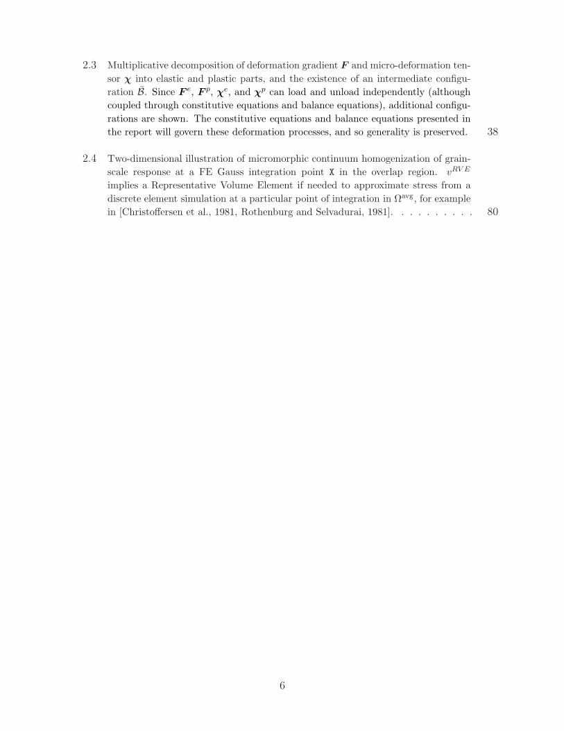
2.3 Multiplicative decomposition of deformation gradient F and micro-deformation ten-
sor χ into elastic and plastic parts, and the existence of an intermediate configu-
ration B. Since F e, F p, χe, and χp can load and unload independently (although
coupled through constitutive equations and balance equations), additional configu-
rations are shown. The constitutive equations and balance equations presented in
the report will govern these deformation processes, and so generality is preserved. 38
2.4 Two-dimensional illustration of micromorphic continuum homogenization of grain-
scale response at a FE Gauss integration point X in the overlap region. vRV E
implies a Representative Volume Element if needed to approximate stress from a
discrete element simulation at a particular point of integration in Ωavg, for example
in [Christoffersen et al., 1981, Rothenburg and Selvadurai, 1981]. . . . . . . . . . 80
6

Acknowledgements
This work was supported by the ARMY RESEARCH LABORATORY (Dr. John Clayton)under the auspices of the U.S. Army Research Office Scientific Services Program administeredby Battelle (Delivery Order 0356, Contract No. W911NF-07-D-0001).
7

This page intentionally left blank.
8
Chapter 1
Introduction
1.1 Description of problem
Dynamic failure in bound particulate materials is a combination of physical processes in-
cluding grain and matrix deformation, intra-granular cracking, matrix cracking, and inter-
granular-matrix/binder cracking/debonding, and is influenced by global initial boundary
value problem (IBVP) conditions. Discovering how these processes occur by experimen-
tal measurements is difficult because of their dynamic nature and the influence of global
boundary conditions (BCs). Typically, post-mortem microscopy observations are made of
fractured/fragmented/comminuted material [Kipp et al., 1993], or real-time in-situ infrared-
optical surface observations are conducted of the dynamic failure process [Guduru et al.,
2001]. These observation techniques, however, miss the origins of dynamic failure internally
in the material. Under quasi-static loading conditions, non-destructive high spatial resolu-
tion (a few microns) synchrotron micro-computed tomography can be conducted [Fredrich
et al., 2006]∗ to track three-dimensionally the internal grain-scale fracture process leading
to macro-cracks (though these cracks can propagate unstably). Dynamic loading, however,
can generate significantly-different micro-structural response, usually fragmented and com-
minuted material [Kipp et al., 1993]. Global BCs, such as lateral confinement on cylindrical
compression specimens, also can influence the resulting failure mode, generating in a glass
ceramic composite axial splitting and fragmentation when there is no confinement and shear
fractures with confinement [Chen and Ravichandran, 1997]. Thus, we resort to physics-based
∗Such experimental techniques are not yet mature, but can provide meaningful insight into the origins of‘static’ fracture, and thus could play an important role in the discovery of the origins of dynamic failure.
9

CHAPTER 1. INTRODUCTION
modeling to help uncover these origins dynamically.
Examples of bound particulate materials include, but are not limited to, the following: poly-
crystalline ceramics (crystalline grains with amorphous grain boundary phases, Fig.1.1(a)),
metal matrix composites (metallic grains with bulk amorphous metallic binder, Fig.1.1(b)),
particulate energetic materials (explosive crystalline grains with polymeric binder, Fig.1.1(c)),
asphalt pavement (stone/rubber aggregate with hardened binder, Fig.1.1(d)), mortar (sand
grains with cement binder), conventional quasi-brittle concrete (stone aggregate with cement
binder), and sandstones (sand grains with clayey binder). Bound particulate materials con-
tain grains (quasi-brittle or ductile) bound by binder material oftentimes called the “matrix.”
The heterogeneous particulate nature of these materials governs their mechanical behavior
at the grain-to-macro-scales, especially in IBVPs for which localized deformation nucleates.
Thus, grain-scale material model resolution is needed in regions of localized deformation nu-
cleation (e.g., at a macro-crack tip, or at the high shear strain rate interface region between
a projectile and target material†). To predict dynamic failure for realistic IBVPs, a model-
ing approach will need to account simultaneously for the underlying grain-scale physics and
macro-scale continuum IBVP conditions.
Traditional single-scale continuum constitutive models have provided the basis for under-
standing the dynamic failure of these materials for IBVPs on the macro-scale [Rajendran
and Grove, 1996, Dienes et al., 2006, Johnson and Holmquist, 1999], but cannot predict dy-
namic failure because they do not account explicitly for the material’s particulate nature.
Direct Numerical Simulation (DNS) represents directly the grain-scale mechanical behavior
under static [Caballero et al., 2006] and dynamic loading conditions [Kraft et al., 2008, Kraft
and Molinari, 2008]. Currently, DNS is the best approach to understanding fundamentally
dynamic material failure, but is deficient in the following ways: (i) it is limited by current
computing power (even massively-parallel computing) to a small representative volume el-
ement (RVE) of the material; and (ii) it usually must assume unrealistic BCs on the RVE
(e.g., periodic, or prescribed uniform traction or displacement). Thus, multi-scale modeling
techniques are needed to predict dynamic failure in bound particulate materials.
Current multi-scale approaches attempt to do this but fall short by one or more of the
following limitations: (i) not providing proper BCs on the micro-structural DNS region
†Both projectile and target material could be modeled with such grain-scale material model resolutionat their interface region where significant fracture and comminution occurs. We will start by assuming theprojectile is a deformable solid continuum body without grain-scale resolution, and then extend to includesuch resolution in the future.
10

1.1. DESCRIPTION OF PROBLEM
(a) (b)
(c) (d)
Figure 1.1. (a) Microstructure of alumina, composed of grains bound by glassy phase. (b) SiCreinforced 2080 aluminum metal matrix composite [Chawla et al., 2004]. The 4 black squares areindents to identify the region. (c) Cracking in explosive HMX grains and at grain-matrix interfaces[Baer et al., 2007]. (d) Cracking in asphalt pavement.
(called “unit cell” by Feyel and Chaboche [2000], extended to account for discontinuities
in Belytschko et al. [2008]); (ii) homogenizing at the macro-scale the underlying micro-
structural response in the unit cell and thus not maintaining a computational ‘open window’
to model micro-structurally dynamic failure‡; and (c) not making these methods adaptive,
i.e., moving a computational ‘open window’ with grain-scale model resolution over regions
experiencing dynamic failure.
Feyel and Chaboche [2000] and Belytschko et al. [2008] recognized the complexities and
‡This is a problem especially for modeling fragmentation and comminution micro-structurally.
11

CHAPTER 1. INTRODUCTION
limitations of unit cell methods as they are currently formulated, implemented, and applied.
Feyel [2003] stated that, in addition to the periodicity assumption for the micro-structure
(impossible to model fracture), “... real structures have edges, either external or internal
ones (in case of a multimaterial structure). In the present FE2 framework, nothing has been
done to treat such effects. As a consequence, one cannot expect a good solution near edges.
This is clearly a weak point of the approach ...” In fact, for a non-periodic heterogeneous
micro-structure found in bound particulate materials, we should not expect predictive results
for modeling nucleation of fracture anywhere in the unit cell.
Belytschko et al. [2008] introduced discontinuities into Feyel and Chaboche [2000]’s unit
cell (calling it a “perforated unit cell”) and relaxed the periodicity assumption to model
fracture nucleation, while up-scaling the effects of unit cell discontinuities to the macro-scale
to obtain global cracks embedded in the FE solution (using the extended finite element
method). BCs on the unit cell are an issue, as well as the interaction of adjacent unit cells.
As noted in Belytschko et al. [2008], if regular displacement BCs (i.e., no jumps) are applied
to unit cells that are fracturing, then the fracture is constrained non-physically. Belytschko
et al. [2008] proposed to address this issue by solving iteratively for displacement BCs by
applying a traction instead. What traction to apply is still an unknown and can be provided
by the coarse-scale FE solution. Belytschko et al. [2008] stated that “... the application
of boundary conditions on the unit cell and information transfer to/from the unit cell pose
several difficulties ... When the unit cell localizes, prescribed linear displacements as given
in the analysis are not compatible with the discontinuities ... The effects of boundaries and
adjacent discontinuities are not reflected in the method.”
1.2 Proposed Approach
A finite strain micromorphic plasticity model framework [Regueiro, 2010] is applied to formu-
late a simple pressure-sensitive plasticity model to account for the underlying microstructural
mechanical response in bound particulate materials (pressure-sensitive heterogeneous mate-
rials). Linear isotropic elasticity and non-associative Drucker-Prager plasticity with cohesion
hardening/softening are assumed for the constitutive equations [Regueiro, 2009]. Micromor-
phic continuum mechanics is used in the sense of Eringen [1999]. This was found to be
one of the more general higher order continuum mechanics frameworks for accounting for
underlying microstructural mechanical response. Until this work, however, the finite
12

1.3. FOCUS OF REPORT
strain formulation based on multiplicative decomposition of the deformation gra-
dient F and micro-deformation tensor χ has not been presented in the literature
with sufficient account of the reduced dissipation inequality and conjugate plas-
tic power terms to dictate the plastic evolution equation forms. We provide such
details in this report.
To illustrate the application of the micromorphic plasticity model to the problem of interest,
we refer to an illustration in Fig.1.2 of a concurrent multiscale modeling framework for
bound particulate materials (target) impacted by a deformable solid (projectile). The higher
order continuum micromorphic plasticity model is used in the overlap region between a
continuum finite element (FE) and DNS representation of the particulate material. The
additional degrees of freedom provided by the micromorphic model (micro-shear, micro-
dilation/compaction, and micro-rotation) will allow the overlap region to be placed closer
to the region of interest, such as at a projectile-target interface. Further from this interface
region, standard continuum mechanics and constitutive models can be used.
1.3 Focus of Report
Regarding the approach described in Sect.1.2, this Report focusses primarily on the nonlin-
ear micromorphic continuum mechanics and finite strain elastoplasticity constitutive model
tasks. How this generalized continuum model couples via an overlapping region to the DNS
region (Fig.1.2) is described in Sects.2.4,2.5.
An outline of the report is as follows: Section 2.1 summarizes the Statement of Work (SOW)
and the Tasks, 2.2 presents the formulation of the nonlinear (finite deformation) micromor-
phic continuum mechanics balance equations, 2.3 presents the finite strain elastoplasticity
modeling framework based on a multiplicative decomposition of the deformation gradient
and micro-deformation tensor, Sects.2.4 and 2.5 describe how the micromorphic continuum
mechanics fits into a multiscale modeling approach, and Chapt.3 summarizes the results,
conclusions, and future work.
13

CHAPTER 1. INTRODUCTION
particulate micro-structural DNS region
(DE and/or FE/CSE)
micromorphic continuum FE region
coupling region
(micromorphic continuum FE
to particulate micro-structural DNS)
deformable solid body (projectile)
continuum FE mesh
bound particulate material (target)
multi-scale computational modelv
Figure 1.2. 2D illustration of concurrent computational multi-scale modeling approach in thecontact interface region between a bound particulate material (e.g., ceramic target) and deformablesolid body (e.g., refractory metal projectile). The discrete element (DE) and/or finite element (FE)representation of the particulate micro-structure is intentionally not shown in order not to clutterthe drawing of the micro-structure. The grains (binder matrix not shown) of the micro-structureare ‘meshed’ using DEs and/or FEs with cohesive surface elements (CSEs). The open circles denotecontinuum FE nodes that have prescribed degrees of freedom (dofs) D based on the underlyinggrain-scale response, while the solid circles denote continuum FE nodes that have free dofs Dgoverned by the micromorphic continuum model. We intentionally leave an ‘open window’ (i.e.,DNS) on the particulate micro-structural mesh in order to model dynamic failure. If the continuummesh overlays the whole particulate micro-structural region, as in Klein and Zimmerman [2006] foratomistic-continuum coupling, then the continuum FEs would eventually become too deformed byfollowing the micro-structural motion during fragmentation. The blue-dashed box at the bottom-center of the illustration is a micromorphic continuum FE region that can be converted to a DNSregion for adaptive high-fidelity material modeling as the projectile penetrates the target.
1.4 Notation
Cartesian coordinates are assumed for easier presentation of concepts and also to be able to
define a Lagrangian elastic strain measure Eein the intermediate configuration B, assuming a
multiplicative decomposition of the deformation gradient F and micro-deformation tensor χ
14

1.4. NOTATION
into elastic and plastic parts (Sect.2.3.1). See Regueiro [2010] for more details regarding finite
strain micromorphic elastoplasticity in general curvilinear coordinates, and also Eringen
[1962] for nonlinear continuum mechanics in general curvilinear coordinates, and Clayton
et al. [2004, 2005] for nonlinear crystal elastoplasticity in general curvilinear coordinates.
Index notation will be used mostly so as to be as clear as possible with regard to details of
the formulation. Cartesian coordinates are assumed, so all indices are subscripts, and spatial
partial derivative is the same as covariant derivative [Eringen, 1962]. Some symbolic/direct
notation is also given, such that (ab)ik = aijbjk, (a ⊗ b)ijkl = aijbkl, (a ⊙ c)ijk = aimcjmk.
Boldface denotes a tensor or vector, where its index notation is given. Generally, variables in
uppercase letters and no overbar live in the reference configuration B0 (such as the reference
differential volume dV ), variables in lowercase live in the current configuration B (such
as the current differential volume dv), and variables in uppercase with overbar live in the
intermediate configuration B (such as the intermediate differential volume dV ). The same
applies to their indices, such that a differential line segment in the current configuration
dxi is related to a differential line segment in the reference configuration dXI through the
deformation gradient: dxi = FiIdXI (Einstein’s summation convention assumed [see Eringen,
1962, Holzapfel, 2000]). In addition, the multiplicative decomposition of the deformation
gradient is written as FiI = F eiIF p
II(F = F eF p), where superscripts e and p denote elastic
and plastic parts, respectively. Subscripts (•),i (•),I and (•),I imply spatial partial derivatives
in the current, intermediate, and reference configurations, respectively. A superscript prime
symbol (•)′ denotes a variable associated with the micro-element for micromorphic continuum
mechanics. Superposed dot ˙(2) = D(2)/Dt denotes material time derivative. The symboldef= implies a definition.
15

Chapter 2
Technical Discussion
2.1 Statement of Work (SOW) and Specific Tasks
Bound particulate materials are commonly found in industrial products, construction ma-
terials, and nature (e.g., geological materials). They include polycrystalline ceramics (e.g.,
crystalline grains with amorphous grain boundary phases), energetic materials (high explo-
sives and solid rocket propellant), hot asphalt, asphalt pavement (after asphalt has cured),
mortar, conventional quasi-brittle concrete, ductile fiber composite concretes, and sand-
stones, for instance. Bound particulate materials contain particles∗ (quasi-brittle or ductile)
bound by binder material oftentimes called the “matrix”.
The heterogeneous nature of bound particulate materials governs its mechanical behavior at
the particle- to continuum-scales. The particle-scale is denoted as the scale at which particle-
matrix mechanical behavior is dominant, thus necessitating that particles and matrix mate-
rial be resolved explicitly (i.e., meshed directly in a numerical model), accounting for their
interfaces and differences in material properties. Currently, there is no approach enabling pre-
diction of initiation and propagation of dynamic fracture in bound particulate materials—for
example polycrystalline ceramics, particulate energetic materials, mortar, and sandstone—
accounting for their underlying particulate microstructure across multiple length-scales con-
currently. Traditional continuum methods have provided the basis for understanding the
dynamic fracture of these materials, but cannot predict the initiation of dynamic fracture
∗We use ‘particle’ and ‘grain’ interchangeably.
16

2.1. STATEMENT OF WORK (SOW) AND SPECIFIC TASKS
without accounting for the material’s particulate nature. Direct numerical simulation (DNS)
of deformation, intra-particle cracking, and inter-particle-matrix/binder debonding at the
particle-scale is limited by current computing power (even massively-parallel computing)
to a small representative volume element (RVE) of the material, and usually must assume
overly-restrictive boundary conditions (BCs) on the RVE (e.g., fixed normal displacement).
Multiscale modeling techniques are clearly needed to accurately capture the response of
bound particulate materials in a way accounting simultaneously for effects of the microstruc-
ture at the particle-scale and boundary conditions applied to the engineering structure of
interest, at the continuum-scale. The services of a scientist or engineer are required to de-
velop the mathematical theory and numerical methodology for multiscale modeling of bound
particulate materials of interest to the Army Research Laboratory (ARL).
The overall objective of the proposed research is to develop a concurrent multi-scale com-
putational modeling approach that couples regions of continuum deformation to regions
of particle-matrix deformation, cracking, and debonding, while bridging the particle- to
continuum-scale mechanics to allow numerical adaptivity in modeling initiation of dynamic
fracture and degradation in bound particulate materials.
For computational efficiency, the solicited research will use DNS only in spatial regions
of interest, such as the initiation site of a crack and its tip during propagation, and a
micromorphic continuum approach will be used in the overlap and adjacent regions to provide
proper BCs on the DNS region, as well as an overlay continuum to which to project the
underlying particle-scale mechanical response (stress, internal state variables (ISVs)). The
micromorphic continuum constitutive model will account for the inherent length scale of
damaged fracture zone at the particle-scale, and thus includes the kinematics to enable
the proper coupling with the fractured DNS particle region. Outside of the DNS region, a
micromorphic extension of existing continuum model(s), with the particular model(s) to be
determined based on ARL needs, of material behavior will be used.
This SOW calls for development of the formulation and finite element implementation of
a finite strain micromorphic inelastic constitutive model to bridge particle-scale mechanics
to the continuum-scale. The desired result is formulation of such a model enabling a more
complete understanding of the role of microstructure-scale physics on the thermomechanical
properties and performance of heterogeneous materials of interest to ARL. These materials
could include, but are not limited to, the following: ceramic materials, energetic materials,
geological materials, and urban structural materials.
17

CHAPTER 2. TECHNICAL DISCUSSION
2.1.1 Specific Tasks
Specific tasks, and summary of what was accomplished for each Task.
1. Investigate and assess specific needs of ARL researchers with regards to multi-scale
modeling of heterogeneous particulate materials. Determine, following discussion with
ARL materials researchers, the desired classical continuum constitutive model to be
reformulated as a micromorphic continuum constitutive model and used in the region
outside and overlapping partially the DNS window, for material(s) of interest to ARL.
For example, polycrystalline ceramics models include those of Johnson and Holmquist
[1999] or Rajendran and Grove [1996] and energetic materials include those following
Dienes et al. [2006].
A finite strain Drucker-Prager pressure-sensitive elastoplasticity model [Regueiro, 2009]
was selected as a simple model approximation to start, with future extension to the
more sophisticated constitutive model forms mentioned in the Task 1. This model is
presented in Sect.2.3.3.
2. Formulate theory and numerical algorithms for a finite strain micromorphic inelastic
constitutive model to bridge particle-scale mechanics to the continuum-scale based on
the decided constitutive equations from Task 1.
See summary for Task 1.
3. Initiate finite element implementation of the formulated finite strain micromorphic
inelastic constitutive model in a continuum mechanics code.
The finite element implementation has been initiated in the password-protected ver-
sion of Tahoe tahoe.colorado.edu, where the opensource is available at tahoe.cvs.
sourceforge.net. This report focusses on the theory, while details of finite element
implementation and numerical examples will follow in journal articles and a future
report.
4. Interact with ARL researchers in order to improve mutual understanding (i.e., under-
standing of both PI and of ARL) with regards to dynamic fracture and material degra-
dation in bound particulate materials and associated numerical modeling techniques.
Continue to interact with ARL researchers regarding their needs for this research prob-
lem.
18

2.2. NONLINEAR MICROMORPHIC CONTINUUM MECHANICS
5. Formulate algorithm to couple finite strain micromorphic continuum finite elements to
DNS finite elements of bound particulate material through an overlapping region.
The formulated algorithm is presented in Sect.2.5.
6. Initiate implementation of coupling algorithm in [previous] Task using finite element
code Tahoe (both for micromorphic continuum and DNS). Future extension can be made
for coupling micromorphic model (Tahoe) to DNS model (ARL or other finite element,
or particle/meshfree, code).
The coupling algorithm has been initiated for a finite element and discrete element
coupling. Extension to other DNS models of the grain-scale response is part of future
work. See Sect.2.5.
2.2 Nonlinear micromorphic continuum mechanics
2.2.1 Kinematics
Figure 2.1 illustrates the mapping of the macro-element and micro-element in the refer-
ence configuration to the current configuration through the deformation gradient F and
micro-deformation tensor χ. The macro-element continuum point is denoted by P (X,Ξ)
and p(x, ξ, t) in the reference and current configurations, respectively, with centroid C and
c. The micro-element continuum point centroid is denoted by C ′ and c′ in the reference
and current configurations, respectively. The micro-element is denoted by an assembly of
particles, but in general represents a grain/particle/fiber microstructural sub-volume of the
heterogeneous material. The relative position vector of the micro-element centroid with re-
spect to the macro-element centroid is denoted by Ξ and ξ(X,Ξ, t) in the reference and
current configurations, respectively, such that the micro-element centroid position vectors
are written as (Fig.2.1) [Eringen and Suhubi, 1964, Eringen, 1999]
X ′K = XK + ΞK , x′k = xk(X, t) + ξk(X,Ξ, t) (2.1)
Eringen and Suhubi [1964] assumed that for sufficiently small lengths ‖Ξ‖ ≪ 1 ( ‖ • ‖ is the
L2 norm), ξ is linearly related to Ξ through the micro-deformation tensor χ, such that
19

CHAPTER 2. TECHNICAL DISCUSSION
ξk(X,Ξ, t) = χkK(X, t)ΞK (2.2)
where then the spatial position vector of the micro-element centroid is written as
x′k = xk(X, t) + χkK(X, t)ΞK (2.3)
This is equivalent to assuming an affine, or homogeneous, deformation of the macro-element
differential volume dV (but not the body B; i.e., the continuum body B is expected to
experience heterogeneous deformation because of χ, even if boundary conditions (BCs) are
uniform). It also simplifies considerably the formulation of the micromorphic continuum
balance equations as presented in Eringen and Suhubi [1964], Eringen [1999]. This micro-
deformation χ is analogous to the small strain micro-deformation tensor ψ in Mindlin [1964],
physically described in his Fig.1. Eringen [1968] also provides a physical interpretation of
χ generally, but then simplies for the micropolar case. For example, χ can be interpreted
as calculated from a micro-displacement gradient tensor Φ as χ = 1 + Φ, where Φ is not
actually calculated from a micro-displacement vector u′, but a u′ can be calculated once Φ
is known (see (2.265)). The micro-element spatial velocity vector (holding X and Ξ fixed)
is then written as
v′k = x′k = xk + ξk = vk + νklξl (2.4)
where ξk = χkKΞK = χkKχ−1Klξl = νklξl, vk is the macro-element spatial velocity vector,
νkl = χkKχ−1Kl (ν = χχ−1) the micro-gyration tensor, similar in form to the velocity gradient
vk,l = FkKF−1Kl (ℓ = F F−1).
Now we take the partial spatial derivative of (2.3) with respect to the reference micro-element
position vector X ′K , to arrive at an expression for the micro-element deformation gradient
F ′kK as (see Appendix A)
20

2.2. NONLINEAR MICROMORPHIC CONTINUUM MECHANICS
P (X ,Ξ)
p(x, ξ, t)
X1
X2
X3
C
c
c
C ′
C ′c′
Ξ
Ξξ
X
xX ′
x′
F , χ
F , 1
1, χ
X ′K = XK + ΞK
x′k = xk(X , t) + ξk(X,Ξ, t)
dV
dv
dv
dV ′
dV ′dv′
BB0
Figure 2.1. Map from reference B0 to current configuration B accounting for relative positionΞ, ξ of micro-element centroid C ′, c′ with respect to centroid of macro-element C, c. F and χcan load and unload independently (although coupled through constitutive equations and balanceequations), and thus the additional current configuration is shown.
F ′kK = FkK(X , t) +
∂χkL(X, t)
∂XK
ΞL
+
(χkA(X, t)− FkA(X, t)− ∂χkM(X , t)
∂XA
ΞM
)∂ΞA∂XK
(2.5)
21
CHAPTER 2. TECHNICAL DISCUSSION
where the deformation gradient of the macro-element is FkK = ∂xk(X, t)/∂XK . The micro-
element deformation gradient F ′kK maps micro-element differential line segments dx′k =
F ′kKdX
′K and volumes dv′ = J ′dV ′, where J ′ = detF ′ is the micro-element Jacobian of
deformation. This is presented for generality of mapping stresses between B0 and B, B0 and
B, B and B, but will not be used explicitly in the constitutive equations in Sect.2.3.3.
2.2.2 Micromorphic balance equations and Clausius-Duhem in-
equality
Using the spatial integral-averaging approach in Eringen and Suhubi [1964], we can derive
the balance equations and Clausius-Duhem inequality summarized in (2.57). The rationale of
this integral-averaging approach over dv and B in the current configuration is to assume the
classical balance equations in micro-element differential volume dv′ must hold over integrated
macro-element differential volume dv, in turn integrated over the current configuration of
the body in B. This approach will be applied repeatedly to derive the micromorphic balance
equations in (2.57).
Balance of mass: The micro-element mass m′ over dv can be expressed as
m′ =
∫
dv
ρ′dv′ =
∫
dV
ρ′0dV′ (2.6)
where ρ′0 = ρ′J ′, J ′ = detF ′. Then, the conservation of micro-element mass m′ is
Dm′
Dt= 0 (2.7)
=D
Dt
∫
dv
ρ′dv′ =D
Dt
∫
dV
ρ′J ′dV ′
=
∫
dV
(Dρ′
DtJ ′ + ρ′
DJ ′
Dt
)dV ′
=
∫
dv
(Dρ′
Dt+ ρ′
∂v′l∂x′l
)dv′ = 0
Thus, the pointwise (localized) balance of mass over dv is
22
2.2. NONLINEAR MICROMORPHIC CONTINUUM MECHANICS
Dρ′
Dt+ ρ′
∂v′l∂x′l
= 0 (2.8)
Now, consider the balance of mass of solid over the whole body B. We start with the
integral-average definition of mass density:
ρdvdef=
∫
dv
ρ′dv′ (2.9)
The total mass m of body B is expressed as
m =
∫
B
ρdv =
∫
B
[∫
dv
ρ′dv′]=
∫
B0
[∫
dV
ρ′J ′dV ′
](2.10)
Then for conservation of mass over the body B we have
Dm
Dt=
∫
B0
[∫
dV
D(ρ′J ′)
DtdV ′
]
=
∫
B
∫
dv
Dρ′
Dt+ ρ′
∂v′l∂x′l︸ ︷︷ ︸
=0
dv′
= 0 (2.11)
Then, the balance of mass in B leads to the standard result
Dm
Dt=
D
Dt
∫
B
ρdv = 0
=
∫
B0
D(ρJ)
DtdV
=
∫
B
(Dρ
Dt+ ρ
∂vl∂xl
)dv = 0 (2.12)
Localizing the integral we have the pointwise satisfaction of balance of mass for a single
23

CHAPTER 2. TECHNICAL DISCUSSION
constituent (in this case, solid) material:
Dρ
Dt+ ρ
∂vl∂xl
= 0 (2.13)
Balance of micro-inertia:
Given that ΞK is the position of micro-element dV ′ centroid C ′ in the reference configuration
with respect to the mass center of the macro-element dV centroid C (see Fig.2.1), we have
the result
∫
dV
ρ′0ΞKdV′ = 0 (2.14)
This can be thought of as the first mass moment being zero because of the definition ΞK as
the “relative” position of C ′ with respect to C (the mass center of dV ) [Eringen, 1999]. The
second mass moment is not zero, and in the process a micro-inertia IKL in B0 is defined as
ρ0IKLdVdef=
∫
dV
ρ′0ΞKΞLdV′ (2.15)
Likewise, a micro-inertia ikl in B is defined as
ρikldvdef=
∫
dv
ρ′ξkξldv′ (2.16)
=
∫
dv
ρ′χkKΞKχlLΞLdv′
= χkKχlL
∫
dv
ρ′0ΞKΞLdV′
= χkKχlLρ0IKLdV = χkKχlLρIKLdv
=⇒ IKL = χ−1Kkχ
−1Ll ikl (2.17)
The balance of micro-inertia in B0 is then defined as
24

2.2. NONLINEAR MICROMORPHIC CONTINUUM MECHANICS
D
Dt
∫
B0
ρ0IKLdV =
∫
B0
ρ0DIKLDt
dV = 0 (2.18)
DIKLDt
= χ−1Kkχ
−1Ll
(DiklDt
− νkaial − νlaiak
)
=
∫
B
ρχ−1Kkχ
−1Ll
(DiklDt
− νkaial − νlaiak
)dv = 0
Localizing the integral, and factoring out ρχ−1Kkχ
−1Ll , the pointwise balance of micro-inertia in
B is
DiklDt
− νkaial − νlaiak = 0 (2.19)
Balance of linear momentum, and first moment of momentum: To derive the micromorphic
balance of linear momentum and first moment of momentum (different than angular mo-
mentum), Eringen and Suhubi [1964] followed a weighted residual approach, where the point
of departure is that balance of linear and angular momentum in the micro-element dv′ over
dv are satisfied:
σ′lk,l + ρ′(f ′
k − a′k) = 0 (2.20)
σ′lk = σ′
kl (2.21)
where micro-element Cauchy stress σ′ is symmetric (macro-element Cauchy stress σ will
be shown to be symmetric). Using a smooth weighting function φ′ (to be defined for three
cases), the weighted average over B of the balance of linear momentum on dv is expressed
as
∫
B
∫
dv
φ′[σ′lk,l + ρ′(f ′
k − a′k)]dv′
= 0 (2.22)
where (•)′,l = ∂(•)′/∂x′l. Applying the chain rule (φ′σ′lk),l = φ′
,lσ′lk + φ′σ′
lk,l, we can rewrite
(2.22) as
25

CHAPTER 2. TECHNICAL DISCUSSION
∫
B
∫
dv
[(φ′σ′
lk),l − φ′,lσ
′lk + ρ′φ′(f ′
k − a′k)]dv′
= 0 (2.23)
∫
∂B
∫
da
(φ′σ′lk)n
′lda
′
+
∫
B
∫
dv
[−φ′
,lσ′lk + ρ′φ′(f ′
k − a′k)]dv′
= 0 (2.24)
We consider three cases for the weighting function φ′ leading to three separate micromorphic
balance equations on B:
1. φ′ = 1, balance of linear momentum
2. φ′ = enmkx′m, balance of angular momentum, where enmk is the permutation tensor
[Holzapfel, 2000]
3. φ′ = x′m, balance of first moment of momentum
Substituting these three choices for φ′ into (2.24), we can derive the respective micromorphic
balance equations on B:
1. φ′ = 1, balance of linear momentum:
∫
∂B
∫
da
σ′lkn
′lda
′
+
∫
B
∫
dv
[ρ′(f ′k − a′k)] dv
′
= 0 (2.25)
The spatial-averaged definitions of unsymmetric Cauchy stress σlk, body force fk, and
acceleration ak are used to derive the micromorphic balance of linear momentum:
σlknldadef=
∫
da
σ′lkn
′lda
′ (2.26)
ρfkdvdef=
∫
dv
ρ′f ′kdv
′ (2.27)
ρakdvdef=
∫
dv
ρ′a′kdv′ (2.28)
From (2.25) and (2.26-2.28), there results
26
2.2. NONLINEAR MICROMORPHIC CONTINUUM MECHANICS
∫
∂B
σlknlda+
∫
B
ρ(fk − ak)dv = 0 (2.29)∫
B
[σlk,l + ρ(fk − ak)] dv = 0 (2.30)
Localizing the integral, we have the pointwise expression for micromorphic balance of
linear momentum
σlk,l + ρ(fk − ak) = 0 (2.31)
Note that the macroscopic Cauchy stress σlk is unsymmetric.
2. φ′ = enmkx′m, x
′m = xm + ξm, balance of angular momentum:
∫
∂B
∫
da
enmk(x′mσ
′lk)n
′lda
′
+
∫
B
∫
dv
enmk[−x′m,lσ′
lk + ρ′x′m(f′k − a′k)
]dv′
= 0
∫
∂B
∫
da
enmk((xm + ξm)σ′lk)n
′lda
′
+
∫
B
∫
dv
enmk [−σ′mk + ρ′(xm + ξm)(f
′k − a′k)] dv
′
= 0 (2.32)
where x′m,l = ∂x′m/∂x′l = δml. We analyze the terms in (2.32), using a′k = ak + ξk and
ξk = (νkc + νkbνbc)ξc, such that
27
CHAPTER 2. TECHNICAL DISCUSSION
∫
∂B
∫
da
enmk((xm + ξm)σ′lk)n
′lda
′
=
∫
∂B
enmkxm
∫
da
σ′lkn
′lda
′
︸ ︷︷ ︸def= σlknlda
+
∫
∂B
enmk
∫
da
σ′lkξmn
′lda
′
︸ ︷︷ ︸def=mlkmnlda
= enmk
∫
∂B
[xmσlknl +mlkmnl] da
= enmk
∫
B
[σmk + xmσlk,l +mlkm,l] dv (2.33)
∫
B
∫
dv
enmk [−σ′mk] dv
′
= −enmk
∫
B
∫
dv
σ′mkdv
′
︸ ︷︷ ︸def= smkdv
= −enmk∫
B
smkdv (2.34)
∫
B
∫
dv
enmk [ρ′(xm + ξm)f
′k] dv
′
=
∫
B
enmkxm
∫
dv
ρ′f ′kdv
′
︸ ︷︷ ︸def= ρfkdv
+
∫
B
enmk
∫
dv
ρ′f ′kξmdv
′
︸ ︷︷ ︸def= ρℓkmdv
= enmk
∫
B
(xmρfk + ρℓkm) dv (2.35)
∫
B
∫
dv
enmk [ρ′(xm + ξm)(−a′k)] dv′
= −enmk
∫
B
∫
dv
ρ′(xmak + xmξk + ξmak
+ξmξk)dv′
= −enmk∫
B
xmak
∫
dv
ρ′dv′
︸ ︷︷ ︸def= ρdv
+xm(νkc + νkbνbc)
∫
dv
ρ′ξcdv′
︸ ︷︷ ︸=0
+ak
∫
dv
ρ′ξmdv′
︸ ︷︷ ︸=0
+
∫
dv
ρ′ξkξmdv′
︸ ︷︷ ︸def= ρωkmdv
= −enmk∫
B
[xmρak + ρωkm] dv (2.36)
where mlkm is the higher order (couple) stress, smk is the symmetric micro-stress, ℓkm
28

2.2. NONLINEAR MICROMORPHIC CONTINUUM MECHANICS
is the body force couple, and ωkm is the micro-spin inertia. Combining the terms, we
have
enmk
∫
B
xm(σlk,l + ρ(fk − ak)︸ ︷︷ ︸
=0
) + σmk − smk +mlkm,l + ρ(ℓkm − ωkm)
dv = 0
enmk
∫
B
[σmk − smk +mlkm,l + ρ(ℓkm − ωkm)] dv = 0 (2.37)
Thus, upon localizing the integral,
enmk [σmk − smk +mlkm,l + ρ(ℓkm − ωkm)] = 0 (2.38)
σ[mk] − s[mk]︸︷︷︸=0
+ml[km],l + ρ(ℓ[km] − ω[km]) = 0 (2.39)
resulting in
σ[mk] +ml[km],l + ρ(ℓ[km] − ω[km]) = 0 (2.40)
where the antisymmetric definition σ[mk] = (σmk − σkm)/2. Eq(2.40) is the pointwise
balance of angular momentum on B, providing 3 equations to solve for a micro-rotation
vector ϕk [Eringen, 1968]. But we want to solve for the general nine-dimensional micro-
deformation tensor χkK , thus we need 6 more equations. The balance of first moment
of momentum provides these additional equations.
3. φ′ = x′m, balance of first moment of momentum: The analysis follows that for balance
of angular momentum, except we do not multiply by the permutation tensor enmk.
Thus, we may write directly (2.38) without enmk as
σmk − smk +mlkm,l + ρ(ℓkm − ωkm) = 0 (2.41)
This in general provides 9 equations to solve for a micro-displacement gradient tensor
ΦkK through the definition χkK = δkK +ΦkK . We note that (2.41) encompasses (2.40)
(the 3 antisymmetric equations), and provides 6 additional equations (the symmetric
part of (2.41)) [Eringen and Suhubi, 1964].
29
CHAPTER 2. TECHNICAL DISCUSSION
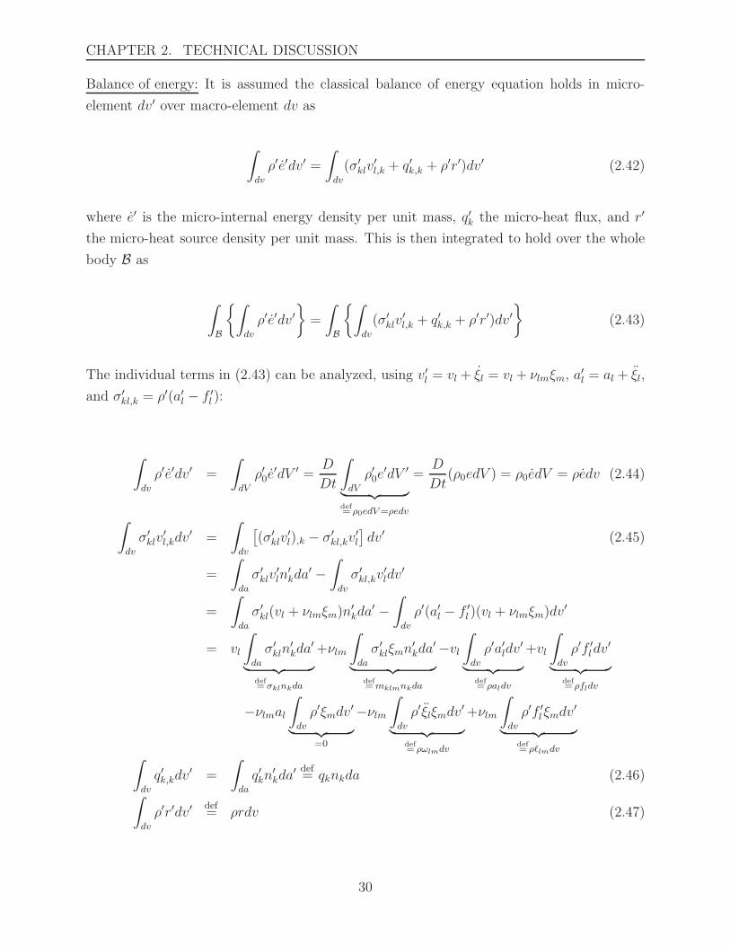
Balance of energy: It is assumed the classical balance of energy equation holds in micro-
element dv′ over macro-element dv as
∫
dv
ρ′e′dv′ =
∫
dv
(σ′klv
′l,k + q′k,k + ρ′r′)dv′ (2.42)
where e′ is the micro-internal energy density per unit mass, q′k the micro-heat flux, and r′
the micro-heat source density per unit mass. This is then integrated to hold over the whole
body B as
∫
B
∫
dv
ρ′e′dv′
=
∫
B
∫
dv
(σ′klv
′l,k + q′k,k + ρ′r′)dv′
(2.43)
The individual terms in (2.43) can be analyzed, using v′l = vl + ξl = vl + νlmξm, a′l = al + ξl,
and σ′kl,k = ρ′(a′l − f ′
l ):
∫
dv
ρ′e′dv′ =
∫
dV
ρ′0e′dV ′ =
D
Dt
∫
dV
ρ′0e′dV ′
︸ ︷︷ ︸def= ρ0edV=ρedv
=D
Dt(ρ0edV ) = ρ0edV = ρedv (2.44)
∫
dv
σ′klv
′l,kdv
′ =
∫
dv
[(σ′
klv′l),k − σ′
kl,kv′l
]dv′ (2.45)
=
∫
da
σ′klv
′ln
′kda
′ −∫
dv
σ′kl,kv
′ldv
′
=
∫
da
σ′kl(vl + νlmξm)n
′kda
′ −∫
dv
ρ′(a′l − f ′l )(vl + νlmξm)dv
′
= vl
∫
da
σ′kln
′kda
′
︸ ︷︷ ︸def= σklnkda
+νlm
∫
da
σ′klξmn
′kda
′
︸ ︷︷ ︸def=mklmnkda
−vl∫
dv
ρ′a′ldv′
︸ ︷︷ ︸def= ρaldv
+vl
∫
dv
ρ′f ′ldv
′
︸ ︷︷ ︸def= ρfldv
−νlmal∫
dv
ρ′ξmdv′
︸ ︷︷ ︸=0
−νlm∫
dv
ρ′ξlξmdv′
︸ ︷︷ ︸def= ρωlmdv
+νlm
∫
dv
ρ′f ′l ξmdv
′
︸ ︷︷ ︸def= ρℓlmdv∫
dv
q′k,kdv′ =
∫
da
q′kn′kda
′ def= qknkda (2.46)
∫
dv
ρ′r′dv′def= ρrdv (2.47)
30

2.2. NONLINEAR MICROMORPHIC CONTINUUM MECHANICS
Substituting these terms back into (2.43), we have
∫
B
ρedv =
∫
∂B
(vlσklnk + νlmmklmnk)da−∫
B
vlρ(al − fl)dv −∫
B
νlmρ(ωlm − ℓlm)dv
+
∫
∂B
qknkda+
∫
B
ρrdv (2.48)
=
∫
B
vl(σkl,k + ρ(fl − al)︸ ︷︷ ︸
=0
) + νlm(mklm,k + ρ(ℓlm − ωlm)︸ ︷︷ ︸=sml−σml
)
+vl,kσkl + νlm,kmklm + qk,k + ρr] dv
Localizing the integral, the pointwise balance of energy over B becomes
ρe = νlm(sml − σml) + vl,kσkl + νlm,kmklm + qk,k + ρr (2.49)
Second Law of Thermodynamics and Clausius-Duhem Inequality: We assume the second law
is valid in micro-element dv′ over dv such that
D
Dt
∫
dv
ρ′η′dv′
︸ ︷︷ ︸∫dvρ′η′dv′
def= ρηdv
−∫
da
1
θq′kn
′kda
′
︸ ︷︷ ︸∫dv
(q′kθ),kdv′
def= (
qkθ),kdv
−∫
dv
ρ′r′
θdv′
︸ ︷︷ ︸def= ρr
θdv
≥ 0 (2.50)
Note that no micro-temperature θ′ is currently introduced [Eringen, 1999]. Integrating over
B, localizing the integral, and multiplying by macro-temperature θ, we arrive at the pointwise
form of the second law as
∫
B
ρηdv −∫
B
(1
θqk,k −
qkθ2θ,k
)dv −
∫
B
ρr
θdv ≥ 0 (2.51)
ρθη − qk,k +1
θqkθ,k − ρr ≥ 0 (2.52)
We derive the micromorphic Clausius-Duhem inequality by introducing the Helmholtz free
31

CHAPTER 2. TECHNICAL DISCUSSION
energy function ψ, and using the balance of energy in (2.49). Recall the definition of ψ
[Holzapfel, 2000], and its material time derivative leading to an expression for ρθη in (2.52)
as
ψ = e− θη (2.53)
ψ = e− θη − θη (2.54)
ρθη = ρe− ρθη − ρψ (2.55)
Upon substitution into (2.52) and using (2.49), we arrive at the micromorphic Clausius-
Duhem inequality:
−ρ(ψ + ηθ) + σkl(vl,k − νlk) + sklνlk +mklmνlm,k +1
θqkθ,k ≥ 0 (2.56)
32
2.2. NONLINEAR MICROMORPHIC CONTINUUM MECHANICS
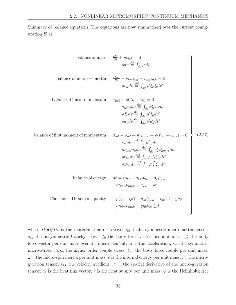
Summary of balance equations: The equations are now summarized over the current config-
uration B as
balance of mass : Dρ
Dt+ ρvk,k = 0
ρdvdef=∫dvρ′dv′
balance of micro − inertia : DiklDt
− νkmiml − νlmimk = 0
ρikldvdef=∫dvρ′ξkξldv
′
balance of linearmomentum : σlk,l + ρ(fk − ak) = 0
σlknldadef=∫daσ′lkn
′lda
′
ρfkdvdef=∫dvρ′f ′
kdv′
ρakdvdef=∫dvρ′a′kdv
′
balance of firstmoment of momentum : σml − sml +mklm,k + ρ(ℓlm − ωlm) = 0
smldvdef=∫dvσ′mldv
′
mklmnkdadef=∫daσ′klξmn
′kda
′
ρℓlmdvdef=∫dvρ′f ′
l ξmdv′
ρωlmdvdef=∫dvρ′ξlξmdv
′
balance of energy : ρe = (skl − σkl)νlk + σklvl,k
+mklmνlm,k + qk,k + ρr
Clausius −Duhem inequality : −ρ(ψ + ηθ) + σkl(vl,k − νlk) + sklνlk
+mklmνlm,k +1θqkθ,k ≥ 0
(2.57)
where D(•)/Dt is the material time derivative, ikl is the symmetric micro-inertia tensor,
σlk the unsymmetric Cauchy stress, fk the body force vector per unit mass, f ′l the body
force vector per unit mass over the micro-element, ak is the acceleration, sml the symmetric
micro-stress, mklm the higher order couple stress, ℓlm the body force couple per unit mass,
ωlm the micro-spin inertia per unit mass, e is the internal energy per unit mass, νlk the micro-
gyration tensor, vl,k the velocity gradient, νlm,k the spatial derivative of the micro-gyration
tensor, qk is the heat flux vector, r is the heat supply per unit mass, ψ is the Helmholtz free
33

CHAPTER 2. TECHNICAL DISCUSSION
energy per unit mass, η is the entropy per unit mass, and θ is the absolute temperature. Note
that the balance of first moment of momentum is more general than the balance of angular
momentum (or “moment of momentum” [Eringen, 1962]), such that its skew-symmetric part
is the angular momentum balance of a micropolar continuum (see above (2.40)). Recall that
the Cauchy stress σ′ml over the micro-element is symmetric because the balance of angular
momentum is satisfied over the micro-element [Eringen and Suhubi, 1964].
da
da′
n
n′
Figure 2.2. Differential area of micro-element da′ within macro-element da in current configurationB.
Physically, the micro-stress s defined in (2.57)4 as the volume average of the Cauchy stress
σ′ over the micro-element, can be interpreted in the context of its difference with the un-
symmetric Cauchy stress as s− σ (Mindlin [1964] called this the “relative stress”). This is
the energy conjugate driving stress for the micro-deformation χ through its micro-gyration
tensor ν = χχ−1 in (2.57)5, and also the reduced dissipation inequality in the intermediate
configuration (2.95) and (2.98) as Σ − S (the analogous stress difference in B). In fact,
we do not solve for s or Σ directly, but constitutively we solve for the difference s − σ
or Σ − S (see (2.118)). The higher order stress m is analogous to the double stress µ in
Mindlin [1964] with physical components of micro-stretch, micro-shear, and micro-rotation
34
2.3. FINITE STRAIN MICROMORPHIC ELASTOPLASTICITY
shown in his Fig.2. For example, m112 is the higher order shear stress in the x2 direc-
tion based on a stretch in the x1 direction. Using the area average definition for mklm, we
have m112n1def= (1/da)
∫daσ′11ξ2n
′1da
′, where σ′11 is the normal micro-element stress in the x1
direction, and ξ2 is the shear couple in the x2 direction.
2.3 Finite strain micromorphic elastoplasticity
This section proposes a phenomenological bridging-scale constitutive modeling framework
in the context of finite strain micromorphic elastoplasticity based on a multiplicative de-
composition of the deformation gradient F and micro-deformation tensor χ into elastic and
plastic parts. In addition to the 3 translational displacement vector u degrees of freedom
(dofs), there are 9 dofs associated with the unsymmetric micro-deformation tensor χ (micro-
rotation, micro-stretch, and micro-shear). We leave the formulation general in terms of χ,
which can be further simplified depending on the material and associated constitutive as-
sumptions (see Forest and Sievert [2003, 2006]). The Clausius-Duhem inequality formulated
in the intermediate configuration yields the mathematical form of three levels of plastic
evolutions equations in either (1) Mandel-stress form [Mandel, 1974], or (2) an alternate
‘metric’ form. For demonstration of the micromorphic elastoplasticity modeling framework,
J2 flow plasticity and linear isotropic elasticity are initially assumed, extended to a pressure-
sensitive Drucker-Prager plasticity model, and then mapped to the current configuration for
semi-implicit numerical time integration.
The formulation presented here differs from other works on finite strain micromorphic elasto-
plasticity that consider a multiplicative decomposition into elastic and plastic parts [Sansour,
1998, Forest and Sievert, 2003, 2006] and those that do not [Lee and Chen, 2003, Vernerey
et al., 2007].
Sansour [1998] considered a finite strain Cosserat and micromorphic plastic continuum, re-
defining the micromorphic strain measures (see (B.1) in Appendix B) to be invariant with
respect to rigid rotations only, not also translations. Sansour did not extend his formulation
to include details on a finite strain micromorphic elastoplasticity constitutive model formu-
lation, as this report does. Sansour proposed to arrive at the higher-order macro-continuum
by integrally-averaging micro-continuum plasticity behavior using computation. Such an
approach is similar to computational homogenization, as proposed by Forest and Sievert
[2006] to estimate material parameters for generalized continuum plasticity models. On a
35

CHAPTER 2. TECHNICAL DISCUSSION
side note, one advantage to the micromorphic continuum approach by Eringen and Suhubi
[1964] is that the integral-averaging of certain stresses, body forces, and micro-inertia terms
are already part of the formulation. This will become especially useful when computa-
tionally homogenizing underlying microstructural mechanical response (e.g., provided by a
microstructural finite element or discrete element simulation) in regions of interest, such as
overlapping between micromorphic continuum and grain/particle/fiber representations for a
concurrent multiscale modeling approach (Fig.1.2).
Forest and Sievert [2003, 2006] established a hierarchy of elastoplastic models for generalized
continua, including Cosserat, higher grade, and micromorphic at small and finite strain.
Specifically with regard to micromorphic finite strain theory, Forest and Sievert [2003] follows
the approach of Germain [1973], which leads to different stress power terms in the balance of
energy and, in turn, Clausius-Duhem inequality than presented by Eringen [1999]. Also, the
invariant elastic deformation measures do not match the sets (2.89) and (B.1) proposed by
Eringen [1999]. Upon analyzing the change in square of micro-element arc-lengths (ds′)2 −(dS ′)2 between current B and intermediate configurations B (cf. Appendix C), then either
set (2.89) or (B.1) is unique. Forest and Sievert [2003, 2006] proposed to use a mix of
the two sets, i.e. (2.89)1, (B.1)2, and (B.1)3, in their Helmholtz free energy function. When
analyzing (ds′)2−(dS ′)2, they would also need (B.1)1 as a fourth elastic deformation measure.
As Eringen proposed, however, it is more straightforward to use either set (2.89) or (B.1)
when representing elastic deformation. The report presents both sets, but we use (2.89).
Mandel stress tensors are identified in Forest and Sievert [2003, 2006] to use in the plastic
evolution equations. This report presents additional Mandel stresses and considers also an
alternate ‘metric’-form oftentimes used in finite deformation elastoplasticity modeling.
Vernerey et al. [2007] treated micromorphic plasticity modeling similar to Germain [1973]
and Mindlin [1964], which leads to different stress power terms and balance equations than
in Eringen [1999]. The resulting plasticity model form is thus similar to Forest and Sievert
[2003], although does not use a multiplicative decomposition and thus does not assume the
existence of an intermediate configuration. An extension presented by Vernerey et al. [2007]
is to consider multiple scale micromorphic kinematics, stresses, and balance equations, where
the number of scales is a choice made by the constitutive modeler. A multiple scale averaging
procedure is introduced to determine material parameters at the higher scales based on lower
scale response.
In general, in terms of a multiplicative decomposition of the deformation gradient and micro-
deformation, as compared to recent formulations of finite strain micromorphic elastoplasticity
36
2.3. FINITE STRAIN MICROMORPHIC ELASTOPLASTICITY
reported in the literature (just reviewed in preceding paragraphs), we view our approach
to be more in line with the original concept and formulation presented by Eringen and
Suhubi [1964], Eringen [1999], which provide a clear link between micro-element and macro-
element deformation, balance equations, and stresses. Thus, we believe our formulation and
resulting elastoplasticity model framework is more general than what has been presented
previously. The paper by Lee and Chen [2003] also follows closely Eringen’s micromorphic
kinematics and balance laws, but does not treat multiplicative decomposition kinematics and
subsequent constitutive model form in the intermediate configuration, as this report does.
We demonstrate the formulation for three levels of J2 plasticity and linear isotropic elasticity,
as well as pressure-sensitive Drucker-Prager plasticity, and numerical time integration by a
semi-implicit scheme in the current configuration B.
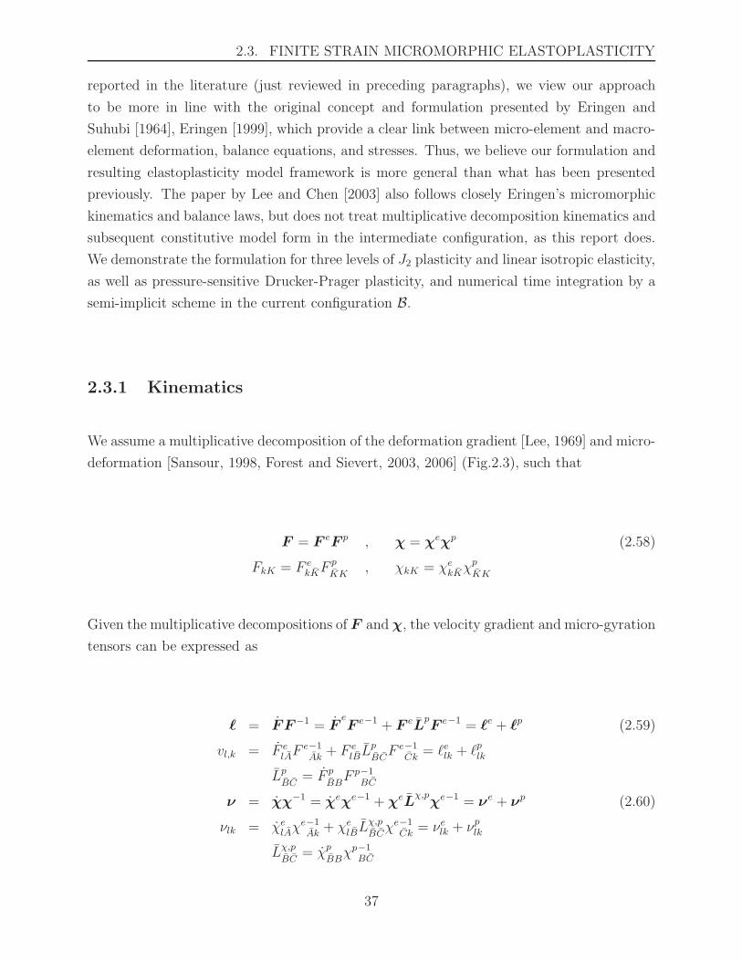
2.3.1 Kinematics
We assume a multiplicative decomposition of the deformation gradient [Lee, 1969] and micro-
deformation [Sansour, 1998, Forest and Sievert, 2003, 2006] (Fig.2.3), such that
F = F eF p , χ = χeχp (2.58)
FkK = F ekKF
p
KK, χkK = χekKχ
p
KK
Given the multiplicative decompositions of F and χ, the velocity gradient and micro-gyration
tensors can be expressed as
ℓ = F F−1 = FeF e−1 + F eL
pF e−1 = ℓe + ℓp (2.59)
vl,k = F elAF
e−1Ak
+ F elBL
p
BCF e−1
Ck= ℓelk + ℓplk
LpBC
= F p
BBF p−1
BC
ν = χχ−1 = χeχe−1 + χeLχ,pχe−1 = νe + νp (2.60)
νlk = χelAχe−1Ak
+ χelBLχ,p
BCχe−1
Ck= νelk + νplk
Lχ,pBC
= χpBBχp−1
BC
37

CHAPTER 2. TECHNICAL DISCUSSION
P
C ′
C ′
Ξ
Ξ
F e, χe
F e, 1
1, χe
F p, χp
F p, 1
1, χp
dV ′
dV ′
dV
dV
P (X ,Ξ)
p(x, ξ, t)
X1
X2
X3
C
C
C
c
c
c
C ′
C ′
C ′
c′
Ξ
Ξ
Ξξ
X
xX ′
x′
F , χ
F , 1
1, χ
dV
dv
dv
dv
dV ′
dV ′
dV ′
dv′
B
B
B0
Figure 2.3. Multiplicative decomposition of deformation gradient F and micro-deformation tensorχ into elastic and plastic parts, and the existence of an intermediate configuration B. Since F e, F p,χe, and χp can load and unload independently (although coupled through constitutive equationsand balance equations), additional configurations are shown. The constitutive equations and bal-ance equations presented in the report will govern these deformation processes, and so generalityis preserved.
In the next section, the Clausius-Duhem inequality requires the spatial derivative of the
micro-gyration tensor, which will be split into elastic and plastic parts based on (2.60).
Thus, it is written as
38

2.3. FINITE STRAIN MICROMORPHIC ELASTOPLASTICITY
∇ν = ∇νe +∇νp (2.61)
νlm,k = νelm,k + νplm,k
νelm,k = χelA,kχe−1Am
− νelnχenD,kχ
e−1Dm
(2.62)
νplm,k =(χelC,k χ
p
CA+ χelE χ
p
EA,k− χelF L
χ,p
F GχpGA,k
)χ−1Am
−νplaχeaA,kχe−1Am
(2.63)
The spatial derivative of the elastic micro-deformation tensor ∇χe is analogous to the small
strain micro-deformation gradient ℵ in Mindlin [1964], and its physical interpretation in Fig.2
of Mindlin [1964]. For example, χe11,2 is an elastic micro-shear gradient in the x2 direction
based on a micro-stretch in the x1 direction. Furthermore, just as differential macro-element
volumes map as
dv = JdV = JeJpdV = JedV (2.64)
where Je = detF e and Jp = detF p, then micro-element differential volumes map as
dv′ = J ′dV ′ = Je′Jp′dV ′ = Je′dV ′ (2.65)
where Je′ = detF e′ and Jp′ = detF p′. F e′ and F p′ have not been defined from (2.5), and are
not required for formulating the final constitutive equations. Likewise, according to micro-
and macro-element mass conservation, mass densities map as
ρ0 = ρJ = ρJeJp = ρJp (2.66)
ρ′0 = ρ′J ′ = ρ′Je′Jp′ = ρ′Jp′ (2.67)
This last result was achieved by using a volume-average definition relating macro-element
mass density to micro-element mass density as
39

CHAPTER 2. TECHNICAL DISCUSSION
ρdvdef=
∫
dv
ρ′dv′ , ρ0dVdef=
∫
dV
ρ′0dV′ , ρdV
def=
∫
dV
ρ′dV ′ (2.68)
This volume averaging approach by Eringen and Suhubi [1964] is used extensively in formu-
lating the balance equations and Clausius-Duhem inequality in Sect.2.2.2.
2.3.2 Clausius-Duhem inequality in B
This section focusses on the Clausius-Duhem inequality mapped to the intermediate config-
uration to identify evolution equations for various plastic deformation rates that must be
defined constitutively, and their appropriate conjugate stress arguments in B.
From a materials modeling perspective, it is oftentimes preferred to write the Clausius-
Duhem inequality in the intermediate configuration B, which is considered naturally elas-
tically unloaded, and formulate constitutive equations there. The physical motivation lies
with earlier work by Kondo [1952], Bilby et al. [1955], Kroner [1960], and others, who viewed
dislocations in crystals as defects with associated local elastic deformation, where macro-
scopic elastic deformation could be applied and removed without disrupting the dislocation
structure of a crystal. More recent models extend this concept, such as papers by Clayton
et al. [2005, 2006] and references therein. The intermediate configuration B can be considered
a “reference” material configuration in which fabric/texture anisotropy and other inelastic
material properties can be defined. Thus, details on the mapping to B are given in this
section. Recall that the Clausius-Duhem inequality in (2.57)6 was written using localization
of an integral over the current configuration B, such that
∫
B
[−ρ(ψ + ηθ) + σkl(vl,k − νlk) + sklνlk +mklmνlm,k +
1
θqkθ,k
]dv ≥ 0 (2.69)
Using the micro-element Piola transform σ′kl = F e′
kKS′KLF e′
lL/Je′ and Nanson’s formula
n′kda
′ = Je′F e′Ak
−1N ′AdA′, the following mappings of the area-averaged unsymmetric Cauchy
stress σ, volume-averaged symmetric micro-stress s, and area-averaged higher order couple
stress m terms are obtained as
40

2.3. FINITE STRAIN MICROMORPHIC ELASTOPLASTICITY
σmlnmdadef=
∫
da
σ′mln
′mda
′
=
∫
dA
1
Je′F e′mM S
′MNF
e′lNJ
e′F e′Am
−1N ′AdA
′
=
∫
dA
F e′lN S
′MNN
′MdA
′
= F elN SMN NMdA
where SMNNMdAdef= F e
Na−1
∫
dA
F e′aBS
′ABN
′AdA
′
recall NMdA =1
JeF emMnmda
=1
JeF emM SMNF
elN︸ ︷︷ ︸
=σml
nmda (2.70)
skldvdef=
∫
dv
σ′kldv
′ =
∫
dV
1
Je′F e′kKS
′KLF
e′lLJ
e′dV ′
= F ekKF
elLΣKLdV
where ΣKLdVdef= F e
Ki−1F e
Lj−1
∫
dV
F e′iIF
e′jJ S
′I JdV
′
=1
JeF ekKΣKLF
elL︸ ︷︷ ︸
=skl
dv (2.71)
41
CHAPTER 2. TECHNICAL DISCUSSION
mklmnkdadef=
∫
da
σ′klξmn
′kda
′
=
∫
dA
1
Je′F e′kKS
′KLF
e′lKχ
emM ΞMJ
e′F e′Ak
−1N ′AdA
′
=
∫
dA
F e′lLχ
emM S
′KLΞMN
′KdA
′
= F elLχ
emMMKLMNKdA
where MKLMNKdAdef= F e
La−1
∫
dA
F e′aBS
′KBΞMN
′KdA
′
recall NKdA =1
JeF ekKnkda
=1
JeF ekKF
elLχ
emMMKLM
︸ ︷︷ ︸=mklm
nkda (2.72)
where S ′KL
is the symmetric second Piola-Kirchhoff stress in the micro-element intermedi-
ate configuration (over dV ), SKL is the unsymmetric second Piola-Kirchhoff stress in the
intermediate configuration B, ΣKL is the symmetric second Piola-Kirchhoff micro-stress in
the intermediate configuration B, MKLM is the higher order couple stress written in the
intermediate configuration, and NK the unit normal on dA. In general, F e′ 6= F e, but the
constitutive equations in Sect.2.3.3 do not require that F e′ be defined or solved.
Using the mappings for ρ and dv, and the Piola transform on qk, the Clausius-Duhem
inequality can be rewritten in the intermediate configuration as
∫
B
[−ρ( ˙ψ + ηθ) + Jeσkl(vl,k − νlk) + Jesklνlk
+νlm,k(F ekKF
elLχ
emMMKLM
)+
1
θQKθ,K
]dV ≥ 0 (2.73)
Individual stress power terms in (2.73) can be additively decomposed into elastic and plastic
parts based on (2.59-2.61). Using (2.61), the higher order couple stress power can be written
as
42

2.3. FINITE STRAIN MICROMORPHIC ELASTOPLASTICITY
νlm,k(F ekKF elLχemM
MKLM
)=
MKLMFelL
(χeaM,K
− νelnχenM,K
)elastic
+MKLMFelL
(−νplnχenM,K
+[χeaC,K
χpCA
+ χeaDχpDA,K
− χeaB Lχ,p
BEχpEA,K
]χp−1
AM
) plastic
(2.74)
where the spatial derivative with respect to the intermediate configuration B can be defined
as
(•),K def= (•),kF e
kK (2.75)
The other stress power terms using (2.59,2.60) are written as
Jeσklvl,k = F ekLF
ekKSKL︸ ︷︷ ︸
elastic
+ CeLBL
p
BKSKL︸ ︷︷ ︸
plastic
(2.76)
Jeσklνlk = (F elLν
elkF
ekK) SKL︸ ︷︷ ︸
elastic
+ ΨeLEL
χ,p
EFχe−1
F kF ekKSKL︸ ︷︷ ︸
plastic
(2.77)
Jesklνlk = (F elLν
elkF
ekK) ΣKL︸ ︷︷ ︸
elastic
+ ΨeLEL
χ,p
EFχe−1
F kF ekKΣKL︸ ︷︷ ︸
plastic
(2.78)
where CeLB
= F eaLF eaB
is the right elastic Cauchy-Green tensor Ce= F eTF e in B, and
ΨeLE
= F elLχ
elE an elastic deformation measure in B as Ψ
e= F eTχe (cf. Appendix C).
Similar to Eringen and Suhubi [1964] for a micromorphic elastic material, the Helmholtz
free energy function in B is assumed to take the following functional form for micromorphic
elastoplasticity as
43

CHAPTER 2. TECHNICAL DISCUSSION
ρψ(F e,χe, ∇χe, Z, Zχ, ∇Z
χ, θ) (2.79)
ρψ(F ekK , χ
ekK, χ
ekM,K , ZK, Z
χ
K, Zχ
K,L, θ)
where ZK is a vector of macro strain-like ISVs in B, Zχ
Kis a vector of micro strain-like ISVs,
and Zχ
K,Lis a spatial derivative of a vector of micro strain-like ISVs. Then, by the chain rule
D(ρψ)
Dt=
∂(ρψ)
∂F ekK
F ekK +
∂(ρψ)
∂χekK
χekK +∂(ρψ)
∂χekM,K
D(χekM,K
)
Dt
+∂(ρψ)
∂ZK
˙ZK +∂(ρψ)
∂Zχ
K
˙ZχK +
∂(ρψ)
∂Zχ
K,L
D(Zχ
K,L)
Dt+∂(ρψ)
∂θθ (2.80)
where an artifact of the “free energy per unit mass” assumption is that
D(ρψ)
Dt= ˙ρψ + ρ ˙ψ = −(ρψ)
Jp
Jp+ ρ ˙ψ =⇒ ρ ˙ψ = (ρψ)
Jp
Jp+D(ρψ)
Dt(2.81)
where we used the result ˙ρ = D(ρ0/Jp)/Dt = −ρJp/Jp. Substituting (2.74-2.78) and
(2.80,2.81) into (2.73), and using the Coleman and Noll [1963] argument for independent
rate processes (independent F ekK
, χekK
, D(χekM,K)/Dt, and θ), the Clausius-Duhem inequal-
ity is satisfied if the following constitutive equations hold:
44

2.3. FINITE STRAIN MICROMORPHIC ELASTOPLASTICITY
SKL =∂(ρψ)
∂F ekK
F e−1Lk
(2.82)
ΣKL =∂(ρψ)
∂F ekK
F e−1Lk
+ F e−1KcχecA
∂(ρψ)
∂χeaA
F e−1La
+F e−1KdχedM ,E
∂(ρψ)
∂χefM ,E
F e−1Lf
(2.83)
MKLM =∂(ρψ)
∂χekM,K
F e−1Lk
(2.84)
ρη = −∂(ρψ)∂θ
(2.85)
For comparison to the result reported in equation (6.3) of Eringen and Suhubi [1964], we
map these stresses to the current configuration, using
σkl =1
JeF ekKSKLF
elL =
1
JeF ekK
∂(ρψ)
∂F elK
(2.86)
skl =1
JeF ekKΣKLF
elL
=1
Je
(F ekK
∂(ρψ)
∂F elK
+ χekA∂(ρψ)
∂χelA
+ χekM,E
∂(ρψ)
∂χelM ,E
)(2.87)
mklm =1
JeF ekKF
elLχ
emMMKLM =
1
Je∂(ρψ)
∂χelM,K
F ekKχ
emM (2.88)
The equations match those in (6.3) of Eringen and Suhubi [1964] if elastic, i.e. F e =
F , χe = χ. We prefer, however, to express the Helmholtz free energy function in terms
of invariant—with respect to rigid body motion on the current configuration B—elastic
deformation measures, such as the set proposed by Eringen and Suhubi [1964] as
CeKL = F e
kKFekL , Ψ
eKL = F e
kKχekL , Γ
eKLM = F e
kKχekL,M (2.89)
We have good physical interpretation of F e (and F p) from crystal lattice mechanics [Bilby
et al., 1955, Kroner, 1960, Lee and Liu, 1967, Lee, 1969], while the elastic micro-deformation
45

CHAPTER 2. TECHNICAL DISCUSSION
χe has its interpretation in Fig.2.3 of this report (elastic deformation of micro-element) and
also Fig.1 of Mindlin [1964] for small strain theory. The spatial derivative of elastic micro-
deformation ∇χe has it physical interpretation in Fig.2 of Mindlin [1964], and was earlier
in this report described, for example, as χe11,2 is the micro-shear gradient in the x2 direction
based on a stretch in the x1 direction (although directions are not exact here because of
the spatial derivative with respect to the intermediate configuration B). The Helmholtz free
energy function ψ per unit mass is then written as
ρψ(Ce, Ψ
e, Γ
e, Z, Z
χ, ∇Z
χ, θ) (2.90)
ρψ(CeKL, Ψ
eKL, Γ
eKLM , ZK, Z
χ
K, Zχ
K,L, θ)
and the constitutive equations for stress result from (2.82-2.84) as
SKL = 2∂(ρψ)
∂CeKL
+∂(ρψ)
∂ΨeKB
Ce−1LA
ΨeAB
+∂(ρψ)
∂ΓeKBC
Ce−1LA
ΓeABC (2.91)
ΣKL = 2∂(ρψ)
∂CeKL
+ 2sym
[∂(ρψ)
∂ΨeKB
Ce−1LA
ΨeAB
]
+2sym
[∂(ρψ)
∂ΓeKBC
Ce−1LA
ΓeABC
](2.92)
MKLM =∂(ρψ)
∂ΓeLMK
(2.93)
where sym [•] denotes the symmetric part. These stress equations (2.91-2.93) when mapped
to the current configuration are the same as equations (6.9-11) in Eringen and Suhubi [1964]
if there is no plasticity, i.e. F e = F and χe = χ. To consider another set of elastic
deformation measures and resulting stresses, refer to Appendix B.
The thermodynamically-conjugate stress-like ISVs are defined as
46
2.3. FINITE STRAIN MICROMORPHIC ELASTOPLASTICITY
QKdef=∂(ρψ)
∂ZK, Qχ
K
def=∂(ρψ)
∂Zχ
K
, Q∇χ
KL
def=
∂(ρψ)
∂Zχ
K,L
(2.94)
which will be used in the evolution equations for plastic deformation rates, as well as multiple
scale yield functions, where we will assume scalar Z, Zχ, ∇Zχ, and Q, Qχ, Q∇χ
. The stress-
like ISVs in Sect.2.3.3 will be physically interpreted as yield stress Q and Qχ for macro-
plasticity (stress S calculated from elastic deformation) and micro-plasticity (stress difference
Σ− S calculated from elastic deformation), respectively, while Q∇χ
is a higher order yield
stress for micro-gradient plasticity (higher order stress M calculated from gradient elastic
deformation).
The remaining terms in the Clausius-Duhem inequality lead to the reduced dissipation in-
equality expressed in localized form in two ways: (1) Mandel form with Mandel-like stresses
[Mandel, 1974], and (2) an alternate ‘metric’ form. Each will lead to different ways of writing
the plastic evolution equations, and stresses that are used in these evolution equations. From
(2.73), the reduced dissipation inequality in Mandel form is written as
−(ρψ) Jp
Jp +1θQKθ,K − QK
˙ZK − Qχ
K˙Zχ
K− Q∇χ
KL
D(Zχ
K,L)
Dt
+(SKBC
eBL
)LpLK
+[Cχ,e−1
KNΨeAN
(ΣAB − SAB)ΨeBL
]Lχ,pLK
+(MKLMΨe
LD
)Lχ,pDM,K
− 2skw[Lχ,pDC
Ψe−1CF
ΓeF MK
]≥ 0
(2.95)
where Cχ,e−1KN
= χe−1Kkχe−1
Nk, Ψe−1
CF= χe−1
CiF e−1
F i, skw [•] denotes the skew-symmetric part
defined as
2skw [•] def=[Lχ,pDC
Ψe−1CF
ΓeF MK
]−[Lχ,pBM
Ψe−1DG
ΓeGBK]
(2.96)
and the spatial derivative of the micro-scale plastic velocity gradient is
Lχ,pDM,K
=[χpDBχp−1
BM
],K
=(χpDB,K
− Lχ,pDB
χpBB,K
)χp−1
BM(2.97)
47
CHAPTER 2. TECHNICAL DISCUSSION
The Mandel stresses are SKBCeBL
, Cχ,e−1KN
ΨeAN
(ΣAB − SAB)ΨeBL
, and MKLMΨeLD
, where the
first one is well-known as the “Mandel stress,” whereas the second and third are the relative
micro-Mandel-stress and the higher order Mandel couple stress, respectively. We rewrite the
reduced dissipation inequality (2.95) in an alternate ‘metric’ form as
−(ρψ) Jp
Jp +1θQKθ,K − QK
˙ZK − Qχ
K˙ZχK − Q∇χ
KL
D(Zχ
K,L)
Dt
+SKL(CeLBLpBK
)+ (ΣKL − SKL)
[ΨeLELχ,pEFCχ,e−1
F NΨeKN
]
+MKLM
ΨeLDLχ,pDM,K
− 2ΨeLD
skw[Lχ,pDC
Ψe−1CF
ΓeF MK
]≥ 0
(2.98)
Form of plastic evolution equations: Based on (2.95), in order to satisfy the reduced dissipa-
tion inequality, we can write plastic evolution equations to solve for F p
KK, χp
KK, and χp
KK,L
in Mandel stress form as
LpLK
= HLK
(SC
e, Q)
(2.99)
solve for F p
KKandF e
kK = FkKFp−1KK
Lχ,pLK
= Hχ
LK
((C
χ,e)−1Ψ
eT (Σ− S)Ψe, Q
χ)(2.100)
solve for χpKK
andχekK = χkKχp−1KK
Lχ,pDM,K
− 2skw[Lχ,pDC
Ψe−1CF
ΓeF MK
]= H∇χ
DMK
(MΨ
e, Q
∇χ)
(2.101)
solve for χpKK,L
andχekK,L = (χkK,L − χekAχp
AK,L)χp−1
KK
where the arguments in parentheses (•) denote the Mandel stress and stress-like ISV to use
in the respective plastic evolution equation, where H , Hχ, and H
∇χdenote tensor functions
for the evolution equations, chosen to ensure that convexity is satisfied, and the dissipation
is positive. This can be seen for the evolution equations in (2.102-2.104) by the constitutive
definitions in (2.120), (2.124), and (2.128) in terms of stress gradients of potential functions
(i.e., the yield functions for associative plasticity). In an alternate ‘metric’ form, from
(2.98), we can solve for the plastic deformation variables as
48
2.3. FINITE STRAIN MICROMORPHIC ELASTOPLASTICITY
CeLBL
p
BK= HLK
(S, Q
)(2.102)
solve for F p
KKandF e
kK = FkKFp−1KK
ΨeLEL
χ,p
EFCχ,e−1
F NΨeKN = Hχ
LK
(Σ− S, Qχ)
(2.103)
solve for χpKK
andχekK = χkKχp−1KK
ΨeLDL
χ,p
DM,K− 2Ψe
LDskw[Lχ,pDC
Ψe−1CF
ΓeF MK
]= H∇χ
LMK
(M , Q
∇χ)
(2.104)
solve for χpKK,L
andχekK,L = (χkK,L − χekAχp
AK,L)χp−1
KK
We use this ‘metric’ form in defining evolution equations in Sect.2.3.3.
Remark 1. The reason that we propose the third plastic evolution equation (2.101) or
(2.104) to solve for χpKK,L
directly (not calculating a spatial derivative of the tensor χpKK
from a finite element interpolation of χp) is to potentially avoid requiring an additional bal-
ance equation to solve in weak form by a nonlinear finite element method (refer to Regueiro
et al. [2007] and references therein). With future finite element implementation and numer-
ical examples, we will attempt to determine whether (2.101) or (2.104) leads to an accurate
calculation of χpKK,L
. In Regueiro [2010], a simpler anti-plane shear version of the model
demonstrates the two ways for calculating ∇χp, either by an evolution equation like in
(2.101) or (2.104), or a finite element interpolation for χp and corresponding gradient cal-
culation ∇χp. Note that in Forest and Sievert [2003], for their equation (155)3, they also
propose a direct evolution of a gradient of plastic micro-deformation.
2.3.3 Constitutive equations
The constitutive equations for linear isotropic elasticity, J2 flow associative plasticity, and
Drucker-Prager non-associative plasticity with scalar ISV hardening/softening are formu-
lated. We define a specific form of the Helmholtz free energy function, yield functions, and
evolution equations for ISVs, and then conduct a semi-implicit numerical time integration
presented in Sect.2.3.4.
49

CHAPTER 2. TECHNICAL DISCUSSION
Linear Isotropic Elasticity and J2 Flow Isochoric Plasticity
Helmholtz free energy and stresses: Assuming linear elasticity and linear relation be-
tween stress-like and strain-like ISVs, a quadratic form for the Helmholtz free energy function
results as
ρψdef=
1
2EeKLAKLMN E
eMN +
1
2EeKLBKLMN EeMN
+1
2ΓeKLM CKLMNP QΓ
eNP Q + Ee
KLDKLMN EeMN
+1
2HZ2 +
1
2Hχ(Zχ)2 +
1
2Zχ
,KH∇χ
KLZχ
,L(2.105)
Note that the ISVs are scalar variables in this model, which will be related to scalar yield
strength of the material at two scales, macro and micro, and H and Hχ are scalar harden-
ing/softening parameters, and H∇χ
KLis a symmetric second order hardening/softening modu-
lus tensor, which we will assume is isotropic as H∇χ
KL= (H∇χ)δKL. Elastic strains are defined
as [Suhubi and Eringen, 1964] 2EeKL
= CeKL
− δKL and EeKL
= ΨeKL
− δKL. The elastic
moduli are defined for isotropic linear elasticity, after manipulation of equations in Suhubi
and Eringen [1964] as
AKLMN = λδKLδMN + µ (δKMδLN + δKNδLM) (2.106)
BKLMN = (η − τ)δKLδMN + κδKMδLN + νδKNδLM
−σ(δKMδLN + δKNδLM) (2.107)
CKLMNP Q = τ1(δKLδMNδP Q + δKQδLMδNP
)
+τ2(δKLδMP δNQ + δKMδLQδN P
)
+τ3δKLδMQδNP + τ4δKNδLMδP Q
+τ5(δKMδLNδP Q + δKP δLMδNQ
)
+τ6δKMδLP δNQ + τ7δKNδLP δMQ
+τ8(δKP δLQδMN + δKQδLNδMP
)+ τ9δKNδLQδMP
+τ10δKP δLNδMQ + τ11δKQδLP δMN (2.108)
DKLMN = τδKLδMN + σ(δKMδLN + δKNδLM) (2.109)
50

2.3. FINITE STRAIN MICROMORPHIC ELASTOPLASTICITY
where AKLMN and DKLMN have major and minor symmetry, while BKLMN and CKLMNP Q
have only major symmetry, and the elastic parameters are λ, µ, η, τ , κ, ν, σ, τ1 . . . τ11. Note
that the units for τ1 . . . τ11 are stress×length2 (e.g., Pa.m2), thus there is a built in length
scale to these elastic parameters for the higher order stress. The elastic modulus tensors
AKLMN , BKLMN , and DKLMN are not the same as in Eringen [1999] because different elastic
strain measures were used, but the higher order elastic modulus tensor CKLMNP Q is the
same. Note that A is the typical linear isotropic elastic tangent modulus tensor, and λ and
µ are the Lame parameters. After some algebra using (2.91-2.94), and (2.105), it can be
shown that the stress constitutive relations are
SKL = AKLMN EeMN + DKBMN EeMN
+(DKBMN EeMN + BKBMN EeMN)
[Ce−1
LAEeAB + δLB
]
+CKBCNP QΓeNP QC
e−1LQ
ΓeQBC (2.110)
ΣKL = AKLMN EeMN + DKBMN EeMN
+2sym(DKLMN E
eMN + BKBMN EeMN)
[Ce−1
LAEeAB + δLB
]
+CKBCNP QΓeNP QC
e−1LQ
ΓeQBC
(2.111)
MKLM = CKLMNP QΓeNP Q (2.112)
Q = HZ (2.113)
Qχ = HχZχ (2.114)
Qχ
L= H∇χZχ
,L(2.115)
Note that the units for H∇χ are stress×length2 (e.g., Pa.m2), thus there is a built in length
scale to this hardening/softening parameter for the higher order stress-like ISV. Assuming
elastic deformations are small, we ignore quadratic terms in (2.110) and (2.111) relative to
the linear terms, leading to the simplified stress constitutive equations for SKL and ΣKL as
51
CHAPTER 2. TECHNICAL DISCUSSION
SKL = (AKLMN + DKLMN)EeMN + (BKLMN + DKLMN )EeMN
= (λ+ τ)(EeMM)δKL + 2(µ+ σ)Ee
KL (2.116)
+η(EeMM)δKL + κEeKL + νEeLKΣKL = (λ+ τ)(Ee
MM)δKL + 2(µ+ σ)EeKL (2.117)
+η(EeMM)δKL + 2sym[κEeKL + νEeLK
]
Note that the stress difference used in (2.103) then becomes
Σ− S = κEeT + νE
e(2.118)
ΣKL − SKL = κEeLK + νEeKL
52

2.3. FINITE STRAIN MICROMORPHIC ELASTOPLASTICITY
Yield functions and evolution equations: In this discussion, three levels of plastic yield
functions are defined based on the three conjugate stress-plastic-power terms appearing in
the reduced dissipation inequality (2.98), with the intent to define the plastic deformation
evolution equations such that (2.98) is satisfied. This allows separate yielding and plastic
deformation at two scales (micro and macro) including the gradient deformation at the
micro-scale. If only one yield function were chosen to be a function of all three stresses
(S, Σ, M), then yielding at the three scales would occur simultaneously, a representation
we feel is not as physical as if the scales can yield and evolve separately (although coupled
through balance equations and stress equations for S and Σ). Recall the plastic power terms
in (2.98) come naturally from the kinematic assumptions F = F eF p and χ = χeχp, and
from the Helmholtz free energy function dependence on the invariant elastic deformation
measures Ce, Ψ
e, Γ
e, and the plastic strain-like ISVs Z, Zχ, and ∇Zχ.
Macro-scale plasticity: For macro-scale plasticity, we write the yield function F as
F (S, α)def= ‖devS‖ − α ≤ 0 (2.119)
‖devS‖ =√(devS) : (devS)
(devS) : (devS) = (devSI J)(devSI J)
devSI Jdef= SI J −
(1
3CeABSAB
)Ce−1
I J
where α is the macro yield strength (i.e., stress-like ISV Qdef= α).
The definitions of the plastic velocity gradient Lpand strain-like ISV then follow as
CeLBL
p
BK
def= ˙γ
∂F
∂SKL(2.120)
∂F
∂SKL= ˆN KL
ˆN KL =devSKL‖devS‖
˙Zdef= − ˙γ
∂F
∂α= ˙γ (2.121)
α = HZ (2.122)
53
CHAPTER 2. TECHNICAL DISCUSSION
where ˙γ is the macro plastic multiplier.
Micro-scale plasticity: For micro-scale plasticity, we write the yield function F χ as
F χ(Σ− S, αχ) def= ‖dev(Σ− S)‖ − αχ ≤ 0 (2.123)
dev(ΣI J − SI J)def= (ΣI J − SI J)−
[1
3CeAB(ΣAB − SAB)
]Ce−1
I J
where αχ is the micro yield strength (stress-like ISV Qχ def= αχ). Note that at the micro-scale,
the yield strength αχ can be determined separately from the macro-scale parameter α.
Remark 2. We use the same functional forms for macro and micro plasticity (F χ with
similar functional form as F , but different ISVs and parameters), but this is only for the
example model presented here. It is possible for the functional forms to be different when
representing different phenomenology at the micro and macro scales. More micromechanical
analysis and experimental data are necessary to determine the micro-plasticity functional
forms in the future.
The definitions of the micro-scale plastic velocity gradient Lχ,p
and strain-like ISV then
follow as
ΨeLEL
χ,p
EFCχ,e−1
F NΨeKN
def= ˙γχ
∂F χ
∂(ΣKL − SKL)(2.124)
∂F χ
∂(ΣKL − SKL)= ˆNχ
KL
ˆNχ
KL=
dev(ΣKL − SKL)
‖dev(Σ− S)‖˙Zχ def
= − ˙γχ∂F χ
∂αχ= ˙γχ (2.125)
αχ = HχZχ (2.126)
54
2.3. FINITE STRAIN MICROMORPHIC ELASTOPLASTICITY
where ˙γχ is the micro plastic multiplier.
Micro-scale gradient plasticity: For micro-scale gradient plasticity, we write the yield function
F∇χ as
F∇χ(M , α∇χ)def= ‖devM‖ − ‖α∇χ‖ ≤ 0 (2.127)
devMI JKdef= MI JK − (Ce−1)IJ
[1
3CeABMABK
]
where α∇χ is the micro gradient yield strength (stress-like ISV Q∇χ def
= α∇χ). Note that at
the gradient micro-scale, the yield strength can be determined separately from the micro- and
macro-scale parameters, which is a constitutive assumption. The definitions of the spatial
derivative of micro-scale plastic velocity gradient ∇Lχ,p
and strain-like ISV then follow as
ΨeLDL
χ,p
DM,K− 2Ψe
LDskw[Lχ,pDC
Ψe−1CF
ΓeF MK
] def= ˙γ∇χ
∂F∇χ
∂MKLM
(2.128)
∂F∇χ
∂MKLM
=devMKLM
‖devM‖D(Zχ
,A)
Dtdef= − ˙γ∇χ
∂F∇χ
∂α∇χ
A
= ( ˙γ∇χ)α∇χ
A
‖α∇χ‖ (2.129)
α∇χ
L= H∇χZχ
,L(2.130)
where ˙γ∇χ is the micro plastic gradient multiplier.
Remark 3. The main advantage to defining constitutively the evolution of the spatial
derivative of micro-scale plastic velocity gradient ∇Lχ,p
in (2.128) separate from the micro-
scale plastic velocity gradient Lχ,p
in (2.124) (i.e., no PDE in χpKK
) is to avoid finite element
solution of an additional balance equation in weak form. One could allow ∇Lχ,p
and ∇˙Zχ
to be defined as the spatial derivatives of Lχ,p
and ˙Zχ, respectively, but then the plastic
evolution equations are PDEs and require coupled finite element implementation (such as in
Regueiro et al. [2007]). We plan to implement the model, after time integration in Sect.2.3.4,
within a coupled finite element formulation for the coupled balance of linear and first moment
55

CHAPTER 2. TECHNICAL DISCUSSION
of momentum, and thus avoiding another coupled equation to include in the finite element
equations is desired.
Remark 4. With these evolution equations in B, (2.120) can be integrated numerically to
solve for F p and in turn F e, (2.124) can be integrated numerically to solve for χp and in
turn χe, and (2.128) can be integrated numerically to solve for ∇χp and in turn ∇χe. Then,
the stresses S, Σ − S, and M can be calculated and mapped to the current configuration
to update the balance equations for finite element nonlinear solution. Such numerical time
integration will be carried out in Sect.2.3.4, and finite element implementation is ongoing
work.
Drucker-Prager Pressure-Sensitive Plasticity
Following the ‘metric’ form in (2.98), the J2 flow plasticity model is generalized to include
pressure-sensitivity of yield and volumetric plastic deformation (dilation only for now, i.e.,
no cap on the yield and plastic potential surfaces that allows plastic compaction, e.g. pore
space collapse).
Macro-scale plasticity: For macro-scale plasticity, we write yield F and plastic potential G
functions as
F (S, c)def= ‖devS‖ −
(Aφc− Bφp
)≤ 0 (2.131)
Aφ = βφ cosφ , Bφ = βφ sin φ , βφ =2√6
3 + β sin φ
‖devS‖ =√
(devS) : (devS)
(devS) : (devS) = (devSI J)(devSI J)
devSI Jdef= SIJ −
(1
3CeABSAB
)Ce−1
IJ
pdef=
1
3CeABSAB =
1
3Ce: S
G(S, c)def= ‖devS‖ −
(Aψc−Bψp
)(2.132)
56

2.3. FINITE STRAIN MICROMORPHIC ELASTOPLASTICITY
where c is the macro cohesion, φ the macro friction angle, ψ the macro dilation angle, and
−1 ≤ β ≤ 1 (β = 1 causes the Drucker-Prager yield surface to pass through the triaxial
extension vertices of the Mohr-Coulomb yield surface, and β = −1 the triaxial compression
vertices). Functional forms of Aψ and Bψ are similar to Aφ and Bφ, respectively, except φ
is replaced with ψ.
The yield and plastic potential functions have the usual functional form for pressure-sensitive
plasticity with cohesive and frictional strength, as well as dilatancy [Desai and Siriwardane,
1984].
Remark 5. To satisfy the reduced dissipation inequality, it can be shown that φ ≥ ψ
[Vermeer and de Borst, 1984] which also has been verified experimentally. We note that
φ > ψ leads to non-associative plasticity, which violates the principle of maximum plastic
dissipation [Lubliner, 1990], but does not violate the reduced dissipation inequality. It is
well known that frictional materials like concrete and rock exhibit non-associative plastic
flow, and thus such feature is also included here. An associative flow rule is reached when
the friction and dilation angles are equal, φ = ψ.
The definitions of the plastic velocity gradient Lpand strain-like ISV then follow as
CeLBL
p
BK
def= ˙γ
∂G
∂SKL(2.133)
∂G
∂SKL= ˆN KL +
1
3BψCe
KL
ˆN KL =devSKL‖devS‖
˙Zdef= − ˙γ
∂G
∂c= Aψ ˙γ (2.134)
c = HZ (2.135)
where ˙γ is the macro plastic multiplier, and the stress-like ISV is Qdef= c.
Remark 6. Note that the functional forms of the plastic evolution equations are similar to
those dictated by the principle of maximum plastic dissipation [Lubliner, 1990], except that
a plastic potential function G is used in place of the yield function F (i.e., non-associative).
57
CHAPTER 2. TECHNICAL DISCUSSION
For purposes of discussion, we show the evolution equations for small strain plasticity:
ǫpdef= γ
∂g
∂σ, ζ
def= −γ ∂g
∂c(2.136)
where ǫp is the plastic strain, and ζ the strain-like ISV. Non-associative plasticity violates
the principle of maximum plastic dissipation, but we use similar functional forms that will
satisfy the reduced dissipation inequality (i.e., the 2nd law of thermodynamics is satisfied).
Micro-scale plasticity: For micro-scale plasticity, we write the yield F χ and plastic potential
Gχ functions as
F χ(Σ− S, cχ) def= ‖dev(Σ− S)‖ −
(Aχ,φcχ −Bχ,φpχ
)≤ 0 (2.137)
Aχ,φ = βχ,φ cosφχ , Bχ,φ = βχ,φ sinφχ , βχ,φ =2√6
3 + βχ sin φχ
dev(ΣI J − SI J)def= (ΣI J − SI J)− pχCe−1
I J
pχdef=
1
3CeAB(ΣAB − SAB)
Gχ(Σ− S, cχ) def= ‖dev(Σ− S)‖ −
(Aχ,ψcχ − Bχ,ψpχ
)(2.138)
where cχ is the micro cohesion, φχ the micro friction angle, ψχ the micro dilation angle, and
−1 ≤ βχ ≤ 1, which are material parameters for the micro-scale. Functional forms of Aχ,ψ
and Bχ,ψ are similar to Aχ,φ and Bχ,φ, respectively, except φχ is replaced with ψχ. Note that
at the micro-scale, the cohesion, friction and dilation angles can be determined separately
from the macro-scale parameters, and likewise the yielding and plastic deformation.
Remark 7. We use the same functional forms for macro and micro plasticity (F χ and Gχ
with similar functional form as F and G), but this is only for the example model presented
here. It is possible for the functional forms to be different when representing different phe-
nomenology at the micro and macro scales. More micromechanical analysis and experimental
data are necessary to determine the pressure-sensitive micro-plasticity functional forms in
the future.
58

2.3. FINITE STRAIN MICROMORPHIC ELASTOPLASTICITY
The definitions of the micro-scale plastic velocity gradient Lχ,p
and strain-like ISV then
follow as
ΨeLEL
χ,p
EFCχ,e−1
F NΨeKN
def= ˙γχ
∂Gχ
∂(ΣKL − SKL)(2.139)
∂Gχ
∂(ΣKL − SKL)= ˆNχ
KL+
1
3Bχ,ψCe
KL
ˆNχ
KL=
dev(ΣKL − SKL)
‖dev(Σ− S)‖˙Zχ def
= − ˙γχ∂Gχ
∂cχ= Aχ,ψ ˙γχ (2.140)
cχ = HχZχ (2.141)
where ˙γχ is the micro plastic multiplier, and Qχ def= cχ.
Micro-scale gradient plasticity: For micro-scale gradient plasticity, we write the yield F∇χ
and plastic potential G∇χ functions as
F∇χ(M , c∇χ)def= ‖devM‖ −
(A∇χ,φ‖c∇χ‖ −B∇χ,φ‖p∇χ‖
)≤ 0 (2.142)
A∇χ,φ = β∇χ,φ cosφ∇χ , B∇χ,φ = β∇χ,φ sinφ∇χ , β∇χ,φ =2√6
3 + β∇χ sinφ∇χ
devMI JKdef= MI JK − Ce−1
I Jp∇χK
p∇χK
def=
1
3CeABMABK
G∇χ(M , c∇χ)def= ‖devM‖ −
(A∇χ,ψ‖c∇χ‖ − B∇χ,ψ‖p∇χ‖
)(2.143)
where c∇χ is the micro gradient cohesion, φ∇χ the micro gradient friction angle, ψ∇χ the
micro gradient dilation angle, and −1 ≤ β∇χ ≤ 1, which are material parameters for the
gradient micro-scale. Functional forms of A∇χ,ψ and B∇χ,ψ are similar to A∇χ,φ and B∇χ,φ,
respectively, except φ∇χ is replaced with ψ∇χ. Note that at the gradient micro-scale, the
cohesion, friction, and dilation angles can be determined separately from the micro- and
macro-scale parameters, which is a constitutive assumption. The definitions of the gradient
of micro-scale plastic velocity gradient ∇Lχ,p
and strain-like ISV then follow as
59

CHAPTER 2. TECHNICAL DISCUSSION
ΨeLDL
χ,p
DM,K− 2Ψe
LDskw[Lχ,pDC
Ψe−1CF
ΓeF MK
] def= ˙γ∇χ
∂G∇χ
∂MKLM
(2.144)
∂G∇χ
∂MKLM
=devMKLM
‖devM‖ +1
3B∇χ,ψCe
KL
p∇χM
‖p∇χ‖˙Zχ
,A
def= − ˙γ∇χ
∂G∇χ
∂c∇χA
= A∇χ,ψ( ˙γ∇χ)c∇χA
‖c∇χ‖ (2.145)
c∇χL
= H∇χZχ
,L(2.146)
where ˙γ∇χ is the micro plastic gradient multiplier.
Remark 8. With these evolution equations in B, (2.133) can be integrated numerically to
solve for F p and in turn F e, (2.139) can be integrated numerically to solve for χp and in
turn χe, and (2.144) can be integrated numerically to solve for ∇χp and in turn ∇χe. Then,
the stresses S, Σ − S, and M can be calculated and mapped to the current configuration
to update the balance equations for finite element nonlinear solution. Such numerical time
integration will be carried out in Sect.2.3.4 for the form of the constitutive equations after
mapping to the current configuration.
Mapping constitutive equations to current configuration B: Oftentimes, the consti-
tutive equations in the intermediate configuration are mapped to the current configuration
Eringen and Suhubi [1964], and the material time derivative is taken to obtain an objective
stress rate and corresponding stress evolution equation in B (cf. Moran et al. [1990], Simo
[1998]). Recall the stress mappings in (2.86-2.88) which when we take the material time
derivative leads to the following equations
σkl = − Je
Jeσkl + ℓekiσil + σkiℓ
eli +
1
JeF e
kK˙SKLF
elL (2.147)
skl = − Je
Jeskl + ℓekisil + skiℓ
eli +
1
JeF e
kK˙ΣKLF
elL (2.148)
mklm = − Je
Jemklm + ℓekimilm +mkimℓ
eli +mkliν
emi +
1
JeF e
kKFelLχ
emM
˙MKLM
(2.149)
60

2.3. FINITE STRAIN MICROMORPHIC ELASTOPLASTICITY
To complete these equations, we need the material time derivative of the stresses in the
intermediate configuration, ˙SKL,˙ΣKL, and
˙MKLM , as well as the mapping of the plastic
evolutions equations to the current configuration. Given the constitutive equation for SKL
in (2.116), we can write
˙SKL = (λ+ τ)( ˙EeMM)δKL + 2(µ+ σ) ˙Ee
KL + η( ˙EeMM)δKL
+κ ˙EeKL + ν ˙EeLK (2.150)
where ˙EeMN
= ˙CeMN
/2 and ˙EeMN
= ˙ΨeMN
. We can show that
˙CeMN = 2F e
iMdeijF
ejN , deij = (ℓeij + ℓeji)/2 , ℓeij = F e
iIFe−1Ij
(2.151)
˙ΨeMN = F e
iMεeijχ
ejN , εeij = νeij + ℓeji , νeij = χeiIχ
e−1Ij
(2.152)
where de is the symmetric elastic deformation rate in B, and εe a mixed micro-macro elastic
velocity gradient in B. Then we can write
F ekK
˙SKLFelL = (λ+ τ)(beijd
eij)b
ekl + 2(µ+ σ)bekid
eijb
ejl + η(ψeijε
eij)b
ekl
+κbekiεeijψ
ejl + νbeliε
eijψ
ejk (2.153)
where the left elastic Cauchy-Green tensor is beij = F eiNF ejN
and a mixed elastic deformation
tensor ψeij = F eiNχejN
. It is then possible to write the material time derivative of the stress
difference map as
F ekK(
˙ΣKL − ˙SKL)FelL = κbeliε
eijψ
ejk + νbekiε
eijψ
ejl (2.154)
For the couple stress, the material time derivative is written as
61

CHAPTER 2. TECHNICAL DISCUSSION
˙MKLM = CKLMNP Q˙ΓeNP Q (2.155)
We can rewrite the gradient of elastic micro-deformation as
ΓeN P Q = F enNγ
enpqχ
epPF
eqQ , γenpq
def= χe−1
ApχenA,q (2.156)
such that
˙ΓeNP Q = F enN
γe
npq χepPF
eqQ (2.157)
γe
npq
def= γenpq + ℓeanγ
eapq + γenpaℓ
eaq + γenaqν
eap (2.158)
Then, the couple stress material time derivative map becomes
F ekKF
elLχ
emM
˙MKLM =[τ1(beklψ
enmψ
eqp + ψelmψ
enpb
ekq
)+ τ2
(beklb
χ,empb
enq + ψekmb
elqψ
enp
)
+τ3beklψ
eqmψ
enp + τ4ψ
elmb
eknψ
eqp + τ5
(ψekmb
elnψ
eqp + ψelmψ
ekpb
enq
)
+τ6ψekmψ
elpb
enq + τ7b
eknψ
elpψ
eqm + τ8
(ψekpb
elqψ
enm + bekqb
elnb
χ,emp
)
+τ9beknb
elqb
χ,emp + τ10ψ
ekpb
elnψ
eqm + τ11b
ekqψ
elpψ
enm
] γe
npq (2.159)
where bχ,emp = χemM
χepM
. In summary, we have the stress evolution equations in B as
62

2.3. FINITE STRAIN MICROMORPHIC ELASTOPLASTICITY
σkl = − Je
Jeσkl + ℓekiσil + σkiℓ
eli +
1
Je[(λ+ τ)(beijd
eij)b
ekl + 2(µ+ σ)bekid
eijb
ejl + η(ψeijε
eij)b
ekl
+κbekiεeijψ
ejl + νbeliε
eijψ
ejk
](2.160)
skl − σkl = − Je
Je(skl − σkl) + ℓeki(sil − σil) + (ski − σki)ℓ
eli +
1
Je(κbeliε
eijψ
ejk + νbekiε
eijψ
ejl) (2.161)
mklm = − Je
Jemklm + ℓekimilm +mkimℓ
eli +mkliν
emi +
1
Je[τ1(beklψ
enmψ
eqp + ψelmψ
enpb
ekq
)+ τ2
(beklb
χ,empb
enq + ψekmbelqψ
enp
)
+τ3beklψ
eqmψ
enp + τ4ψ
elmb
eknψ
eqp + τ5
(ψekmb
elnψ
eqp + ψelmψ
ekpb
enq
)
+τ6ψekmψ
elpb
enq + τ7b
eknψ
elpψ
eqm + τ8
(ψekpb
elqψ
enm + bekqb
elnb
χ,emp
)
+τ9beknb
elqb
χ,emp + τ10ψ
ekpb
elnψ
eqm + τ11b
ekqψ
elpψ
enm
] γe
npq (2.162)
where objective elastic stress rates are defined as
2
σkldef= σkl − ℓekiσil − σkiℓ
eli + deiiσkl (2.163)
2
(skl − σkl)def= (skl − σkl)− ℓeki(sil − σil)− (ski − σki)ℓ
eli + deii(skl − σkl) (2.164)
2
mklmdef= mklm − ℓekimilm −mkimℓ
eli −mkliν
emi + deiimklm (2.165)
where Je/Je = deii. The stress rates on σ and (s−σ) are recognized as the elastic Truesdell
stress rates [Holzapfel, 2000], whereas the stress rate on the higher order stress is new, and
can similarly be defined as an elastic Truesdell higher order stress rate. To show2
m is
objective, consider a rigid body motion [Holzapfel, 2000], with translation c and rotation Q
(orthogonal: QQT = 1) on the current configuration B, resulting in B+, such that
x′+ = c+Q(x+ ξ) = c +Qx′ (2.166)
Recall the definition of the higher order stress through the area-averaging, but now on the
63

CHAPTER 2. TECHNICAL DISCUSSION
translated and rotated configuration B+ as
m+klmn
+k da
def=
∫
da
σ′+kl ξ
+mn
′+k da
′
where σ′+kl = Qkaσ
′abQlb , ξ
+m = Qmcξc , n
′+k = Qkdn
′d
=
∫
da
Qkaσ′abQlbQmcξcQkdn
′dda
′
= Qka
(∫
da
σ′abξcn
′dda
′
)
︸ ︷︷ ︸def=mabcndda
QlbQmcQkd
= QkamabcQlbQmc︸ ︷︷ ︸=m+
klm
n+k da (2.167)
We employ the standard results [Holzapfel, 2000]
ℓe+kl = Ωkl +QkiℓeijQlj (2.168)
νe+kl = Ωkl +QkiνeijQlj (2.169)
de+ii = deii (2.170)
where Ωkl = QkaQla. We substitute into the expression for2
m+, with after some tensor
algebra, we can show that2
m is objective:
2
m+
klm
def= m+
klm − ℓe+ki m+ilm −m+
kimℓe+li −m+
kliνe+mi + de+ii m
+klm
= Qka(mklm − ℓekimilm −mkimℓeli −mkliν
emi + deiimklm)QlbQmc
= Qka
2
mklm QlbQmc (2.171)
q.e.d.
Now, to map the plastic evolution equations, we start with the macro-scale plasticity. The
yield and plastic potential functions in B become
64

2.3. FINITE STRAIN MICROMORPHIC ELASTOPLASTICITY
F (σ, c) = Je‖devσ‖e − Je(Aφc−Bφp
)≤ 0 (2.172)
‖devσ‖e def=√(devσij)be
−1imb
e−1jn (devσmn)
devσij = σij −(1
3σkk
)δij , p =
1
3σkk
G(σ, c) = Je‖devσ‖e − Je(Aψc− Bψp
)(2.173)
where be−1ij = F e−1
MiF e−1
Mj. The map of the plastic velocity gradient and strain-like ISV become
ℓplk = γ∂G
∂σkl(2.174)
∂G
∂σkl= Je
(be−1ka
devσab‖devσ‖e b
e−1bl +
1
3Bψδkl
)
Z = −γ ∂G∂c
= AψγJe (2.175)
c = HZ (2.176)
Next, for micro-scale plasticity, the yield and plastic potential functions in B become
F χ(s− σ, cχ) = Je‖dev(s− σ)‖e − Je(Aχ,φcχ − Bχ,φpχ
)≤ 0 (2.177)
pχ =1
3(skl − σkl)δkl
Gχ(s− σ, cχ) = Je‖dev(s− σ)‖e − Je(Aχ,ψcχ − Bχ,ψpχ
)(2.178)
The map of the plastic micro-gyration tensor and strain-like ISV become
65

CHAPTER 2. TECHNICAL DISCUSSION
νplk = γχ∂Gχ
∂(skl − σkl)(2.179)
∂Gχ
∂(skl − σkl)= Je
(be−1ka
dev(sab − σab)
‖dev(s− σ)‖e be−1bl +
1
3Bχ,ψδkl
)
Zχ = −γχ∂Gχ
∂cχ= Aχ,ψγJe (2.180)
cχ = HχZχ (2.181)
For micro-scale gradient plasticity, the yield and plastic potential functions in B become
F∇χ(m, c∇χ) = Je‖devm‖χ − Je(A∇χ,φ‖c∇χ‖χ −B∇χ,φ‖p∇χ‖χ
)≤ 0 (2.182)
‖c∇χ‖χ def=
√c∇χm bχ,e−1
mnc∇χn
‖devm‖χ def=√
(devmijk)be−1imb
e−1jn b
χ,e−1kp (devmmnp)
‖p∇χ‖χ def=
√p∇χm bχ,e−1
mnp∇χn , p∇χm =
1
3mkkm
G∇χ(m, c∇χ) = Je‖devm‖χ − Je(A∇χ,ψ‖c∇χ‖χ − B∇χ,ψ‖p∇χ‖χ
)(2.183)
The map of the gradient plastic micro-gyration tensor and strain-like ISV become
νplm,k = (γ∇χ)∂G∇χ
∂mklm
(2.184)
∂G∇χ
∂mklm
= Je(
devmabc
‖devm‖χ be−1ka b
e−1lb b
χ,e−1mc +
1
3B∇χ,ψδkl
p∇χa‖p∇χ‖χ b
χ,e−1am
)
Zχ,a = −(γ∇χ)
∂G∇χ
∂c∇χa= A∇χ,ψ(γ∇χ)Je
c∇χb‖c∇χ‖χ b
χ,e−1ba (2.185)
c∇χl = H∇χZχ,ab
χ,eal (2.186)
Remark 9. It is reassuring to see that the left hand sides of the plastic deformation evolu-
tion equations (2.174,2.179,2.184) simplify considerably in the current configuration from the
forms in the intermediate configuration (2.133,2.139,2.144). They will be further simplified
when assuming small elastic deformations.
66
2.3. FINITE STRAIN MICROMORPHIC ELASTOPLASTICITY
Remark 10. Solving numerically for the increment of νplm,k leads to the solution of the
increment of νelm,k, and in turn the evolution of the couple stress mklm over time. We see
this by taking the spatial derivative of the micro-gyration tensor as
νlm,k = νelm,k + νplm,k (2.187)
νlm,k =[χlKχ
−1Km
],k
νelm,k = γelmk − νelaγeamk + νeamγ
elak (2.188)
Remark 11. With the definition of the plastic evolution equations, plastic deformation can
be calculated, and elastic deformation updated to calculate the stresses. A finite element
implementation will solve these equations. We will take advantage of small deformation
elasticity, such that elastic deformation in the current configuration, be−1ij , b
eij , etc, can be
approximated by the second order unit tensor δij .
To illustrate the implementation, we apply assumptions for small elastic deformation in the
next section.
Small elastic deformation and Cartesian coordinates for current configuration B:Assuming small elastic deformation, the tensors be−1
ij , beij, ψ
eij , b
χ,e−1ij ≈ δij and Je ≈ 1,
when multiplied by another variable that is not δij or 1, such as be−1ka devσabb
e−1bl ≈ devσkl.
Also, the rate of elastic volumetric deformation is Je/Je = deii. With these approximations,
in summary, we have the stress evolution equations in B as
67

CHAPTER 2. TECHNICAL DISCUSSION
σkl = −(deii)σkl + ℓekiσil + σkiℓeli + (λ+ τ)(deii)δkl + 2(µ+ σ)dekl
+η(εeii)δkl + κεekl + νεelk (2.189)
skl − σkl = −(deii)(skl − σkl) + ℓeki(sil − σil) + (ski − σki)ℓeli + κεelk + νεekl (2.190)
mklm = −(deii)mklm + ℓekimilm +mkimℓeli +mkliν
emi + cklmnpq
γe
npq
cklmnpq = τ1 (δklδnmδqp + δlmδnpδkq) + τ2 (δklδmpδnq + δkmδlqδnp)
+τ3δklδqmδnp + τ4δlmδknδqp + τ5 (δkmδlnδqp + δlmδkpδnq)
+τ6δkmδlpδnq + τ7δknδlpδqm + τ8 (δkpδlqδnm + δkqδlnδmp)
+τ9δknδlqδmp + τ10δkpδlnδqm + τ11δkqδlpδnm (2.191)
The yield and plastic potential functions in B become
F (σ, c) = ‖devσ‖ −(Aφc− Bφp
)≤ 0 (2.192)
‖devσ‖ =√
(devσij)(devσij)
devσij = σij −(1
3σkk
)δij , p =
1
3σkk
G(σ, c) = ‖devσ‖ −(Aψc−Bψp
)(2.193)
The map of the plastic velocity gradient and strain-like ISV become
ℓplk = γ∂G
∂σkl(2.194)
∂G
∂σkl=
devσkl‖devσ‖ +
1
3Bψδkl
Z = −γ ∂G∂c
= Aψγ (2.195)
c = HZ (2.196)
Notice that ℓp = γ(∂G/∂σ)T . Next, for micro-scale plasticity, the yield and plastic potential
functions in B become
68

2.3. FINITE STRAIN MICROMORPHIC ELASTOPLASTICITY
F χ(s− σ, cχ) = ‖dev(s− σ)‖ −(Aχ,φcχ −Bχ,φpχ
)≤ 0 (2.197)
pχ =1
3(skk − σkk)
Gχ(s− σ, cχ) = ‖dev(s− σ)‖ −(Aχ,ψcχ − Bχ,ψpχ
)(2.198)
The map of the plastic micro-gyration tensor and strain-like ISV become
νplk = γχ∂Gχ
∂(skl − σkl)(2.199)
∂Gχ
∂(skl − σkl)=
dev(skl − σkl)
‖dev(s− σ)‖ +1
3Bχ,ψδkl
Zχ = −γχ∂Gχ
∂cχ= Aχ,ψγχ (2.200)
cχ = HχZχ (2.201)
For micro-scale gradient plasticity, the yield and plastic potential functions in B become
F∇χ(m, c∇χ) = ‖devm‖ −(A∇χ,φ‖c∇χ‖ − B∇χ,φ‖p∇χ‖
)≤ 0 (2.202)
‖c∇χ‖ =
√c∇χm c∇χm
‖devm‖ =√
(devmijk)(devmijk)
devmijk = mijk −1
3δijmaak (2.203)
‖p∇χ‖ =
√p∇χm p∇χm , p∇χm =
1
3mkkm
G∇χ(m, c∇χ) = ‖devm‖ −(A∇χ,ψ‖c∇χ‖ − B∇χ,ψ‖p∇χ‖
)(2.204)
The map of the gradient plastic micro-gyration tensor and strain-like ISV become
69
CHAPTER 2. TECHNICAL DISCUSSION
νplm,k = (γ∇χ)∂G∇χ
∂mklm
(2.205)
∂G∇χ
∂mklm
=devmklm
‖devm‖ +1
3B∇χ,ψδkl
p∇χm‖p∇χ‖
Zχ,a = −(γ∇χ)
∂G∇χ
∂c∇χa= A∇χ,ψ(γ∇χ)
c∇χa‖c∇χ‖ (2.206)
c∇χl = H∇χZχ,l (2.207)
Solving numerically for the increment of νplm,k leads to the solution of the increment of νelm,k,
and in turn the evolution of the couple stress mklm over time. We see this by taking the
spatial derivative of the micro-gyration tensor as
νlm,k = νelm,k + νplm,k (2.208)
νlm,k =[χlKχ
−1Km
],k
νelm,k = γelmk − νelaγeamk + νeamγ
elak
Boxes 1 and 2 provide summaries of the stress and plastic evolution equations, respectively,
in symbolic form to solve numerically in time. The details of the symbolic equations have
been provided in index notation in this Section. The numerical time integration scheme is
presented next in Sect.2.3.4.
70

2.3. FINITE STRAIN MICROMORPHIC ELASTOPLASTICITY
Box 1. Summary of stress evolution equations in the current configuration in symbolic notation.
σ = −(trde)σ + ℓeσ + σℓeT + (λ+ τ)(trde)1+ 2(µ + σ)de
+η(trεe)1+ κεe + νεeT (2.209)
s− σ = −(trde)(s − σ) + ℓe(s− σ) + (s− σ)ℓeT + κεeT + νεe (2.210)
m = −(trde)m+ ℓem+m⊙ ℓeT +mνeT + c...γe
(2.211)
Box 2. Summary of plastic evolution equations in the current configuration in symbolic notation.
ℓp = γ
(∂G
∂σ
)T(2.212)
∂G
∂σ=
devσ
‖devσ‖ +1
3Bψ1 = r
Z = Aψγ (2.213)
νp = γχ(
∂Gχ
∂(s− σ)
)T(2.214)
∂Gχ
∂(s− σ) =dev(s− σ)‖dev(s− σ)‖ +
1
3Bχ,ψ1 = rχ
Zχ = Aχ,ψγ (2.215)
∇νp = (γ∇χ)
(∂G∇χ
∂m
)T(2.216)
∂G∇χ
∂m=
devm
‖devm‖ +1
3B∇χ,ψ1⊗ p∇χ
‖p∇χ‖ = r∇χ
∇Zχ = A∇χ,ψ(γ∇χ)c∇χ
‖c∇χ‖ (2.217)
71
CHAPTER 2. TECHNICAL DISCUSSION
2.3.4 Numerical time integration
The constitutive equations in Sect.2.3.3 are integrated numerically in time following a semi-
implicit scheme [Moran et al., 1990]. We will solve for plastic multiplier increments ∆γ and
∆γχ in a coupled fashion (if yielding is detected at both scales; see Box 9), and multiplier
∆γ∇χ afterward because it is uncoupled. It is uncoupled because of the assumption that
quadratic terms in (2.110) and (2.111) were ignored, leading to uncoupling of the higher
order stress m from Cauchy stress σ and micro-stress s, whereas σ and s remain coupled
(thus coupling γ and γχ).
We assume a deformation-driven time integration scheme within a finite element program
solving the isothermal coupled balance of linear momentum and first moment of momentum
equations (2.57)3 and (2.57)4, respectively, such that deformation gradient F n+1 and micro-
deformation tensor χn+1 are given at time tn+1, as well as their increments ∆F n+1 = F n+1−F n and ∆χn+1 = χn+1 − χn. We assume a time step ∆t = tn+1 − tn. Boxes 3-8 provide
summaries of the semi-implicit time integration of the stress and plastic evolution equations,
respectively, in symbolic form.
To obtain γe in Box 1 throughγe
, we use (2.208) such that
∇ν = ∇νe +∇νp
∇ν = ∇[χχ−1
]
∇νe = γe − νeγe + νeT ⊙ γe
=⇒ γe = νeγe − νeT ⊙ γe +∇ν −∇νp (2.218)
Recall (2.158) which gives the equation for the objective rate of γe as
γedef= γe + ℓeTγe + γeℓe + γe ⊙ νe (2.219)
which appears in (2.211) in Box 1, and in Box 4 for the numerical integration. For ∇(χn+1−χn) and ∇χn+1 in Box 4, because χ is a nodal degree of freedom in a finite element solution
and thus interpolated in a standard fashion, its spatial gradient can be calculated.
72
2.3. FINITE STRAIN MICROMORPHIC ELASTOPLASTICITY
Box 9 summarizes the algorithm for solving the plastic multipliers from evaluating the yield
functions at time tn+1. It involves multiple plastic yield checks, such that macro and/or micro
plasticity could be enabled, and/or micro gradient plasticity. Because the macro and micro
plasticity yield functions F and F χ, respectively, are decoupled from the micro gradient
plastic multiplier γ∇χ, we will solve first for the micro and macro plastic multipliers, as
indicated by (I) in Box 9, and then for the micro gradient plastic multiplier in (II) afterward.
Once the plastic multipliers are calculated, the stresses and ISVs can be updated as indicated
in Boxes 5-8.
This micromorphic plasticity model numerical integration scheme will fit nicely into a cou-
pled Lagrangian finite element formulation and implementation of the balance of linear
momentum and first moment of momentum. Such work is ongoing.
73

CHAPTER 2. TECHNICAL DISCUSSION
Box 3. Summary of semi-implicit time integration of Cauchy stress σ and micro-stress-Cauchy-
stress difference (s − σ) evolution equations. (•)tr implies the trial value, in this case the trial
stress. Results of the semi-implicit time integration of the plastic evolution equations in Box 5 are
included here.
σn+1 = (1− tr(∆tden+1))σn + (∆tℓen+1)σn + σn(∆tℓen+1)T +
(λ+ τ)tr(∆tden+1)1+ 2(µ + σ)(∆tden+1) + ηtr(∆tεen+1)1
+κ(∆tεen+1) + ν(∆tεen+1)T (2.220)
(s− σ)n+1 = (1− tr(∆tden+1))(s − σ)n + (∆tℓen+1)(s− σ)n + (s− σ)n(∆tℓen+1)T +
κ(∆tεen+1)T + ν(∆tεen+1) (2.221)
∆tℓen+1 = ∆tℓn+1 −∆tℓpn+1 (2.222)
∆tℓn+1 = (∆F n+1)F−1n+1
∆tℓpn+1 = (∆γn+1)(r
tr)T , rtr =devσtr
‖devσtr‖ +1
3Bψ1
tr(∆tden+1) = tr(∆tℓn+1)− tr(∆tℓpn+1) = tr(∆tℓn+1)−Bψ(∆γn+1)
∆tεen+1 = ∆tνen+1 +∆tℓeTn+1 (2.223)
∆tνen+1 = ∆tνn+1 −∆tνpn+1
∆tνn+1 = (∆χn+1)χ−1n+1
∆tνpn+1 = (∆γ
χn+1)(r
χ,tr)T , rχ,tr =dev(s− σ)tr‖dev(s− σ)tr‖ +
1
3Bχ,ψ1
tr(∆tεen+1) = tr(∆tεn+1)− tr(∆tεpn+1) = tr(∆tεn+1)−Bχ,ψ(∆γ
χn+1)
tr(∆tεn+1) = tr(∆tνn+1) + tr(∆tℓn+1)
74

2.3. FINITE STRAIN MICROMORPHIC ELASTOPLASTICITY
Box 4. Summary of semi-implicit time integration of higher order stress m evolution equation.
Results of the semi-implicit time integration of the plastic evolution equations in Box 5 are
included here.
mn+1 = (1− tr(∆tden+1))mn + (∆tℓen+1)mn +mn ⊙ (∆tℓen+1)T +mn(∆tνen+1)
T +
c...(∆t
γe
n+1) (2.224)
∆tγe
n+1 = ∆tγen+1 + (∆tℓen+1)Tγen + γ
en(∆tℓen+1) + γ
en ⊙ (∆tνen+1) (2.225)
∆tγen+1 = (∆tνen+1)γen − (∆tνen+1)
T ⊙ γen +∆t∇νn+1 −∆t∇νpn+1 (2.226)
∆t∇νn+1 = ∇(χn+1 − χn)χ−1n+1 − (χn+1 − χn)χ−1
n+1(∇χn+1)χ−1n+1 (2.227)
∆t∇νpn+1 = (∆γ
∇χn+1)(r
∇χ,tr)T (2.228)
r∇χ,tr =devmtr
‖devmtr‖ +1
3B∇χ,ψ1⊗ p∇χ,tr
‖p∇χ,tr‖
75

CHAPTER 2. TECHNICAL DISCUSSION
Box 5. Summary of semi-implicit time integration of plastic evolution equations in the current
configuration.
∆tℓpn+1 = ∆γn+1
(∂G
∂σtr
)T(2.229)
∂G
∂σtr=
devσtr
‖devσtr‖ +1
3Bψ1 = rtr
Zn+1 = Zn +Aψ∆γn+1 (2.230)
cn+1 = HZn+1 (2.231)
∆tνpn+1 = ∆γ
χn+1
(∂Gχ
∂(s− σ)tr)T
(2.232)
∂Gχ
∂(s− σ)tr =dev(s− σ)tr‖dev(s− σ)tr‖ +
1
3Bχ,ψ1 = rχ,tr
Zχn+1 = Zχ
n +Aχ,ψ∆γχn+1 (2.233)
cχn+1 = HχZ
χn+1 (2.234)
∆t∇νpn+1 = (∆γ
∇χn+1)
(∂G∇χ
∂mtr
)T(2.235)
∂G∇χ
∂mtr=
devmtr
‖devmtr‖ +1
3B∇χ,ψ1⊗ p∇χ,tr
‖p∇χ,tr‖ = r∇χ,tr
∇Zχn+1 = ∇Zχ
n +A∇χ,ψ(∆γ∇χn+1)
c∇χn
‖c∇χn ‖(2.236)
c∇χn+1 = H∇χ
∇Zχn+1 (2.237)
76
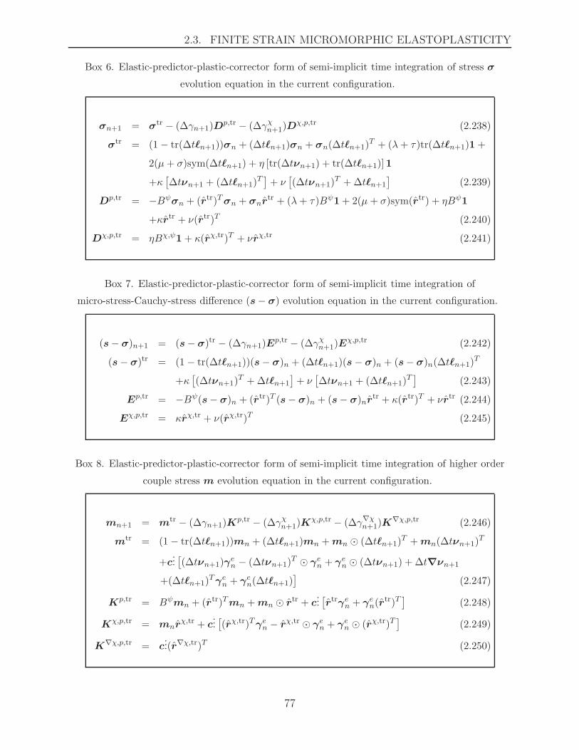
2.3. FINITE STRAIN MICROMORPHIC ELASTOPLASTICITY
Box 6. Elastic-predictor-plastic-corrector form of semi-implicit time integration of stress σ
evolution equation in the current configuration.
σn+1 = σtr − (∆γn+1)Dp,tr − (∆γ
χn+1)D
χ,p,tr (2.238)
σtr = (1− tr(∆tℓn+1))σn + (∆tℓn+1)σn + σn(∆tℓn+1)T + (λ+ τ)tr(∆tℓn+1)1+
2(µ + σ)sym(∆tℓn+1) + η [tr(∆tνn+1) + tr(∆tℓn+1)] 1
+κ[∆tνn+1 + (∆tℓn+1)
T]+ ν
[(∆tνn+1)
T +∆tℓn+1
](2.239)
Dp,tr = −Bψσn + (rtr)Tσn + σnrtr + (λ+ τ)Bψ1+ 2(µ + σ)sym(rtr) + ηBψ1
+κrtr + ν(rtr)T (2.240)
Dχ,p,tr = ηBχ,ψ1+ κ(rχ,tr)T + νrχ,tr (2.241)
Box 7. Elastic-predictor-plastic-corrector form of semi-implicit time integration of
micro-stress-Cauchy-stress difference (s− σ) evolution equation in the current configuration.
(s− σ)n+1 = (s− σ)tr − (∆γn+1)Ep,tr − (∆γ
χn+1)E
χ,p,tr (2.242)
(s− σ)tr = (1− tr(∆tℓn+1))(s− σ)n + (∆tℓn+1)(s − σ)n + (s− σ)n(∆tℓn+1)T
+κ[(∆tνn+1)
T +∆tℓn+1
]+ ν
[∆tνn+1 + (∆tℓn+1)
T]
(2.243)
Ep,tr = −Bψ(s− σ)n + (rtr)T (s− σ)n + (s− σ)nrtr + κ(rtr)T + νrtr (2.244)
Eχ,p,tr = κrχ,tr + ν(rχ,tr)T (2.245)
Box 8. Elastic-predictor-plastic-corrector form of semi-implicit time integration of higher order
couple stress m evolution equation in the current configuration.
mn+1 = mtr − (∆γn+1)Kp,tr − (∆γ
χn+1)K
χ,p,tr − (∆γ∇χn+1)K
∇χ,p,tr (2.246)
mtr = (1− tr(∆tℓn+1))mn + (∆tℓn+1)mn +mn ⊙ (∆tℓn+1)T +mn(∆tνn+1)
T
+c...[(∆tνn+1)γ
en − (∆tνn+1)
T ⊙ γen + γen ⊙ (∆tνn+1) + ∆t∇νn+1
+(∆tℓn+1)Tγen + γ
en(∆tℓn+1)
](2.247)
Kp,tr = Bψmn + (rtr)Tmn +mn ⊙ rtr + c...[rtrγen + γ
en(r
tr)T]
(2.248)
Kχ,p,tr = mnrχ,tr + c
...[(rχ,tr)Tγen − rχ,tr ⊙ γen + γen ⊙ (rχ,tr)T
](2.249)
K∇χ,p,tr = c...(r∇χ,tr)T (2.250)
77

CHAPTER 2. TECHNICAL DISCUSSION
Box 9. Check for plastic yielding and solve for plastic multipliers.
(I) solve for macro and micro plastic multipliers ∆γ and ∆γχ:
Step 1. Compute trial stresses σtr, (s− σ)tr, and trial yield functions F tr, Fχ,tr
Step 2. Consider 3 cases:
(i) If F tr > 0 and Fχ,tr > 0, solve for ∆γn+1 and ∆γχn+1 using Newton-Raphson for
coupled equations:
F (σn+1, cn+1) = F (∆γn+1,∆γχn+1) = 0 (2.251)
Fχ((s − σ)n+1, cχn+1) = Fχ(∆γn+1,∆γ
χn+1) = 0 (2.252)
(ii) If F tr > 0 and Fχ,tr < 0, solve for ∆γn+1 with ∆γχn+1 = 0 using Newton-Raphson:
F (σn+1, cn+1) = F (∆γn+1,∆γχn+1 = 0) = 0 (2.253)
(iii) If F tr < 0 and Fχ,tr > 0, solve for ∆γχn+1 with ∆γn+1 = 0 using Newton-Raphson:
Fχ((s− σ)n+1, cχn+1) = Fχ(∆γn+1 = 0,∆γ
χn+1) = 0 (2.254)
(II) solve for micro gradient plastic multiplier ∆γ∇χ, given ∆γ and ∆γχ:
Step 1. Compute trial stress mtr and trial yield function F∇χ,tr
Step 2. If F∇χ,tr > 0, solve for ∆γ∇χn+1 using Newton-Raphson:
F∇χ(mn+1, c∇χn+1) = F∇χ(∆γ
∇χn+1) = 0 (2.255)
78

2.4. UPSCALING FROM GRAIN-SCALE TO MICROMORPHICELASTOPLASTICITY
2.4 Upscaling from grain-scale to micromorphic elasto-
plasticity
In the overlapping domain, the continuum-scale micromorphic solution can be calculated
as a partly-homogenized representation of the grain-scale solution (Fig.2.4)†. This will be
useful for fitting micromorphic material parameters, and also in estimating DNS material
parameters when converting from micromorphic continuum finite element (FE) mesh to
DNS in a future adaptive scheme. Thus, a micromorphic continuum-scale field 2micromorphic
is defined as a weighted average (over volume and area) of the corresponding field 2grain at
the grain-scale, which is written as follows:
2micromorphic,vol def
=⟨2
grain⟩v
def=
1
vω,avg
∫
Ωavg
ω(r, θ, ϑ)2graindv (2.256)
2micromorphic,arean
def=⟨2
grainngrain⟩a
def=
1
Γavg
∫
Γavg
2grainngrainda (2.257)
where 〈•〉v denotes the volume-averaging operator, vω,avgdef=∫Ωavg ω(r, θ, ϑ)dv the weighted
average current volume, ω(r, θ, ϑ) the kernel function (if using spherical coordinates in 3D
averaging), Ωavg the grain-scale volume averaging domain, 〈•〉a denotes the area-averaging
operator, and Γavg the grain-scale area averaging domain. These averaging operators will be
mapped back to the reference configuration, such that the domains Ωavg0 and Γavg
0 are fixed.
A length ℓ (approximate diameter of Ωavg and Γavg) is a material property and is directly
related to the length scale used in the micromorphic constitutive model.
A macro-element material point (Figs.2.3,2.4) can be characterized as fully overlapping, non-
overlapping, or partly-overlapping according to the level of overlapping between the averaging
domain Ωavg and the full grain-scale DNS region Ωgrain. Within the fully-overlapping aver-
aging domain, the Cauchy stress tensor σgrainkl and vector of ISVs qgraina at the grain-scale will
be projected to the micromorphic continuum-scale using the averaging operators⟨2
grain⟩v
and⟨2
grain⟩ato define the unsymmetric Cauchy stress σkl, the symmetric micro-stress skl,
and the higher order stress mklm:
†The author would like to acknowledge discussions with his colleague at UCB, Prof. F. Vernerey, regardingthe natural built-in homogenization in micromorphic continuum theories of Eringen [1999], Eringen andSuhubi [1964].
79
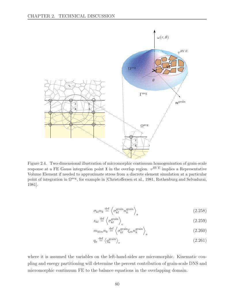
CHAPTER 2. TECHNICAL DISCUSSION
X
X
X
X
X
X
X
X
X
rξ
θ
vRV E
Γavg
ngrain
Ωavg
Ωavg
ω(r, θ)
Figure 2.4. Two-dimensional illustration of micromorphic continuum homogenization of grain-scale
response at a FE Gauss integration point X in the overlap region. vRV E implies a RepresentativeVolume Element if needed to approximate stress from a discrete element simulation at a particularpoint of integration in Ωavg, for example in [Christoffersen et al., 1981, Rothenburg and Selvadurai,1981].
σklnkdef=⟨σgrainkl ngrain
k
⟩a
(2.258)
skldef=⟨σgrainkl
⟩v
(2.259)
mklmnkdef=⟨σgrainkl ξmn
graink
⟩a
(2.260)
qadef=⟨qgraina
⟩v
(2.261)
where it is assumed the variables on the left-hand-sides are micromorphic. Kinematic cou-
pling and energy partitioning will determine the percent contribution of grain-scale DNS and
micromorphic continuum FE to the balance equations in the overlapping domain.
80
2.5. COUPLED FORMULATION
2.5 Coupled formulation
We consider here the bridging-scale decomposition [Kadowaki and Liu, 2004, Klein and
Zimmerman, 2006, Wagner and Liu, 2003] to provide proper BC constraints on a DNS
region to remove fictitious boundary forces and wave reflections.
Kinematics:
The kinematics of the coupled regions are given, following the illustration shown in Fig.1.2.
It is assumed that the micromorphic continuum-FE mesh covers the domain of the problem
in which the bound particulate mechanics is not significantly dominant, whereas in regions
of significant grain-matrix debonding or intra-granular cracking leading to a macro-crack, a
grain-scale mechanics representation is used (grain-FE or grain-DE-FE). Following some of
the same notation presented in Kadowaki and Liu [2004], Wagner and Liu [2003], grain-FE
displacements in the system in the current configuration B are defined as
Q = [qα, qβ, . . . , qγ]T , α, β, . . . , γ ∈ A (2.262)
where qα is the displacement vector of grain-FE node α, and A is the set of all grain-FE
nodes. The micromorphic continuum-FE nodal displacements da and micro-displacement-
gradients φd (see below for χh = 1+Φh [Eringen, 1968]) are written as
D = [da,db, . . . ,dc,φd,φe, . . . ,φf ]T (2.263)
a, b, . . . , c ∈ N , d, e, . . . , f ∈ M
where da is the displacement vector at node a, φd is the micro-displacement-gradient ma-
trix at node d, N is the set of all nodes, and M is the set of finite element nodes with
micro-displacement-gradient dofs, where typically M ⊂ N . In order to satisfy the BCs for
both regions, the motion of the grain-FE nodes in the overlap region (referred to as “ghost”
grain-FE nodes, Fig.1.2) is prescribed by the micromorphic continuum displacement and
micro-displacement-gradient fields, and written as Q ∈ A, while the unprescribed (or free)
grain-FE nodal displacements are Q ∈ A, where A ∪ A = A and A ∩ A = ∅. The displace-
ments and micro-displacement-gradients of continuum-FE nodes overlaying the grain-FE are
driven by the grain-FE motion (also through the averaging shown in Fig.2.4) and written as
D ∈ N ,M, while the unprescribed (or free) nodal displacements and micro-displacement-
81
CHAPTER 2. TECHNICAL DISCUSSION
gradients are D ∈ N ,M, where N ∪N = N , N ∩N = ∅, M∪M = M, and M∩M = ∅.
In general, the displacement vector of a grain-FE node α can be represented by the finite
element interpolation of the continuum macro-displacement field uh and micro-displacement-
gradient field Φh (where χh = 1 + Φh [Eringen, 1968]) evaluated at the grain-FE node in
the reference configuration Xα, such that
uh(Xα, t) =∑
a∈N
Nua (Xα)da(t) , Φh(Xα, t) =
∑
b∈M
NΦb (Xα)φb(t) α ∈ A (2.264)
where Nua are the shape functions associated with the continuum displacement field uh, and
NΦb the shape functions associated with the continuum micro-displacement-gradient field
Φh. Recall that Nua and NΦ
b have compact support and thus are evaluated only for grain-FE
nodes that lie within a micromorphic continuum element containing nodes a and b in its
domain. The displacement of a micro-element (Fig.2.1) can be written as
u′(X,Ξ, t) = x′(X,Ξ, t)−X ′(X,Ξ)
= x(X, t) + ξ(X,Ξ, t)−X − Ξ
= x(X, t)−X︸ ︷︷ ︸u(X ,t)
+ ξ(X,Ξ, t)︸ ︷︷ ︸χ(X ,t)Ξ
−Ξ
= u(X, t) + [χ(X, t)− 1]︸ ︷︷ ︸Φ(X ,t)
Ξ
= u(X, t) +Φ(X, t)Ξ (2.265)
where we used the definition χ = 1+Φ [Eringen, 1968] to put the form of micro-deformation
tensor χ similar to the deformation gradient F = 1+∂u/∂X . The prescribed displacement
of ghost grain-FE node α can then be written as
qα(t) = (u′)h(Xα,Ξα, t) = uh(Xα, t) +Φh(Xα, t)Ξα α ∈ A (2.266)
where Ξα is the relative position of grain-FE node α from a micromorphic continuum point.
The choice of this continuum point could be either a continuum-FE node or Gauss inte-
gration point. This will be investigated in the multiscale implementation. The influence
82
2.5. COUPLED FORMULATION
of the micro-displacement-gradient tensor Φh in the overlap region on the ghost grain-FE
nodal displacement could, through specific micromorphic viscoelastic constitutive relations
for χe, act to “damp out” high-frequency waves propagating through the fine mesh grain-FE
region to the overlap/coupling region. The partitioning of potential and kinetic energies be-
tween grain-FE and micromorphic-continuum-FE systems within the overlap region will be
dependent on the grain-FE equations of the bound particulate system and the micromorphic
continuum-FE equations of the continuum system.
For all ghost grain-FE nodes, the interpolations can be written as
Q =N QD ·D +N QD · D (2.267)
where NQD
and NQD
are shape function matrices containing individual nodal shape func-
tions Nua and NΦ
b , but for now these matrices will be left general to increase our flexibility
in choosing interpolation/projection functions (such as those used in meshfree methods).
Overall, the grain-FE displacements may be written as
[Q
Q
]=
[NQD NQD
N QD N QD
]·[D
D
]+
[Q′
0
](2.268)
where Q′ is introduced [Klein and Zimmerman, 2006] as the error (or “fine-scale” [Wagner
and Liu, 2003]) in the interpolation of the free grain-FE displacements Q, whose function
space is not rich enough to represent the true free grain-FE nodal motion. The shape function
matrices N are in general not square because the number of free grain-FE nodes are not the
same as free micromorphic-FE nodes and prescribed nodes, and number of ghost grain-FE
nodes not the same as prescribed and free micromorphic-FE nodes. A scalar measure of
error in grain-FE nodal displacements is defined as [Klein and Zimmerman, 2006]
e = Q′ ·Q′ (2.269)
which may be minimized with respect to prescribed continuum micromorphic-FE nodal dofs
D to solve for D in terms of free grain-FE nodal dofs and micromorphic continuum FE
nodal dofs as
83

CHAPTER 2. TECHNICAL DISCUSSION
D =M−1
DDNT
QD(Q−NQDD) , M DD =NT
QDNQD (2.270)
This is known as the “discretized L2 projection” [Klein and Zimmerman, 2006] of the free
grain-FE nodal motion Q and free micromorphic-FE nodal dofs D onto the prescribed
micromorphic-FE nodals dofs D. Upon substituting (2.270) into (2.267), we may write the
prescribed grain-FE nodal dofs Q in terms of free grain-FE nodal Q and micromorphic-FE
nodal D dofs. In summary, these relations are written as
Q = BQQQ+BQDD (2.271)
D = BDQQ+B
DDD (2.272)
where
BQQ = N QDBDQ (2.273)
BQD = N QD +N QDBDD (2.274)
BDQ
= M−1
DDNT
QD(2.275)
BDD = −M−1
DDNT
QDNQD (2.276)
As shown in Fig.1.2, for a finite element implementation of this dof coupling, we expect that
free grain-FE nodal dofs Q will not fall within the support of free micromorphic continuum
FE nodal dofs D, such that it can be assumed that NQD = 0 and
Q = BQQQ+BQDD (2.277)
D = BDQQ (2.278)
where
84

2.5. COUPLED FORMULATION
BQQ
= NQDBDQ
(2.279)
BQD = N QD (2.280)
BDQ = M−1
DDNT
QD(2.281)
BDD
= 0 (2.282)
The assumption NQD 6= 0 would be valid for a meshfree projection of the grain-FE nodal
motions to the micromorphic-FE nodal dofs, as in Klein and Zimmerman [2006], where we
could imagine that the domain of influence of the meshfree projection could encompass a
free grain-FE node; the degree of encompassment would be controlled by the chosen support
size of the meshfree kernel function. The choice of meshfree projection in Klein and Zim-
merman [2006] was not necessarily to allow Q be projected to D (and vice versa), but to
remove the computationally costly calculation of the inverse M−1
DDin (2.271) and (2.272).
Since we will also be using the Tahoe code TAHOE for the coupled multiscale grain-FE-
micromorphic-FE implementation, where the meshfree projection has been implemented for
atomistic-continuum coupling [Klein and Zimmerman, 2006], we will also consider the mesh-
free projection in the future.
FE Balance Equations:
Following standard finite element methods to formulate the nonlinear dynamic matrix FE
equations, using the dofs defined in the previous section, the balance of linear momentum
for the grain-scale FE is
MQQ+ F INT,Q(Q) = FEXT,Q (2.283)
where MQ is the mass matrix (lumped or consistent [Hughes, 1987]), F INT,Q(Q) the non-
linear internal force vector, and F EXT,Q the external force vector (which could be a function
of Q, but here such dependence is not shown).
For the balance of linear momentum and balance of first moment of momentum in (2.57),
the weak form can be derived following the method of weighted residuals in Hughes [1987]
(details not shown), the Galerkin form expressed, and then the FE matrix equations written
in coupled form as
85
CHAPTER 2. TECHNICAL DISCUSSION
MDD + F INT,D(D) = FEXT,D (2.284)
where MD is the mass and micro-inertia matrix, F INT,D(D) the nonlinear internal force
vector, F EXT,D the external force vector, and D = [dφ]T is the generalized dof vector for
the coupled micromorphic FE formulation.
These FE equations can be written in energy form to make the partitioning of energy in the
next section more straightforward. For the FE matrix form of balance of linear momentum
at the grain-scale, we have
d
dt
(∂TQ
∂Q
)− ∂TQ
∂Q+∂UQ
∂Q= F EXT,Q (2.285)
where TQ is the kinetic energy and UQ the potential energy, such that
TQ =1
2QMQQ
UQ(Q) =
∫ Q
0F INT,Q(S)dS
Carrying out the derivatives in (2.285), and using the Second Fundamental Theorem of
Calculus for ∂UQ/∂Q, leads to (2.283). Likewise, for the coupled micromorphic balance
equations, we have the energy form
d
dt
(∂TD
∂D
)− ∂TD
∂D+∂UD
∂D= FEXT,D (2.286)
where TD is the kinetic energy and UD the potential energy, such that
86
2.5. COUPLED FORMULATION
TD =1
2DMDD
UD(D) =
∫ D
0F INT,D(S)dS
Partitioning of Energy:
We assume the total kinetic and potential energy of the coupled grain-FE-micromorphic-FE
system may be written as the sum of the energies
T (Q, D) = TQ(Q,˙Q(Q, D)) + TD(D,
˙D(Q)) (2.287)
U(Q,D) = UQ(Q, Q(Q,D)) + UD(D, D(Q)) (2.288)
where we have indicated the functional dependence of the prescribed grain-FE nodal dofs and
micromorphic-FE nodal dofs solely upon the free grain-FE nodal dofs and micromorphic-FE
nodal dofs Q and D, respectively. Lagrange’s equations may then be stated as
d
dt
(∂T
∂Q
)− ∂T
∂Q+∂U
∂Q= FEXT,Q
d
dt
(∂T
∂D
)− ∂T
∂D+∂U
∂D= F EXT,D (2.289)
which lead to a coupled system of governing equations (linear and first moment of mo-
mentum) for the coupled grain-FE-micromorphic-FE mechanics. Details of the derivatives,
partitioning coefficients, and numerical examples will follow in a future report and journal
articles.
87
CHAPTER 2. TECHNICAL DISCUSSION
This page intentionally left blank.
88

Chapter 3
Summary
3.1 Results
The schematic for a concurrent multiscale computational modeling approach for simulating
dynamic fracture in bound particulate materials was presented, that will account for grain-
scale micro-cracking influences on macroscale fracture. Details of a finite strain micromorphic
pressure-sensitive Drucker-Prager elastoplastic constitutive model were presented, as well as
its semi-implicit numerical integration. The approach for coupling grain-scale finite element
equations to the macroscale micromorphic finite element equations was presented.
3.2 Conclusions
A three-level (macro, micro, and micro-gradient) micromorphic pressure-sensitive plasticity
model will provide additional flexibility in coupling with grain-scale mechanics in an overlap-
ping region (Fig.1.2) for attempting to account for influences of grain-scale micro-cracking on
macroscale fracture nucleation and propagation under dynamic loading of bound particulate
materials. The thorough formulation of the finite strain micromorphic elastoplastic consti-
tutive equations in the context of nonlinear micromorphic continuum mechanics has been
established, allowing the multiscale framework to stand on a firm footing, which heretofore
was not presented in the literature.
89

CHAPTER 3. SUMMARY
3.3 Future Work
Future work involves completing the finite element implementation of the finite strain micro-
morphic pressure-sensitive Drucker-Prager plasticity model, and coupling via an overlapping
region to the grain-scale finite element mesh where a projectile may impact a bound partic-
ulate materials target (Fig.1.2).
90

Bibliography
M.R. Baer, C.A. Hall, R.L. Gustavsen, D.E. Hooks, and S.A. Sheffield. Isentropic loading
experiments of a plastic bonded explosive and constituents. J. Appl. Phys., 101(3):34906
– 1, 2007.
T. Belytschko, S. Loehnert, and J.-H. Song. Multiscale aggregating discontinuities: A
method for circumventing loss of material stability. Int. J. Numer. Methods Eng., 73:
869–94, 2008.
B.A. Bilby, R. Bullough, and E. Smith. Continuous distributions of dislocations: a new
application of the methods of non-Riemannian geometry. Proc. R. Soc. Lond. A, Math.
Phys. Eng. Sci., 231:263–273, 1955.
A. Caballero, I. Carol, and C.M. Lopez. A meso-level approach to the 3d numerical analysis
of cracking and fracture of concrete materials. Fatigue Fract. Eng. Mater. Struct., 29(12):
979 – 991, 2006. ISSN 8756-758X.
N. Chawla, V.V. Ganesh, and B. Wunsch. Three-dimensional (3d) microstructure visual-
ization and finite element modeling of the mechanical behavior of sic particle reinforced
aluminum composites. Scripta Mater., 51(2):161 – 165, 2004.
W. Chen and G. Ravichandran. Dynamic compressive failure of a glass ceramic under lateral
confinement. J. Mech. Phys. Solids, 45:1303–28, 1997.
J. Christoffersen, M.M. Mehrabadi, and S. Nemat-Nasser. A micromechanical description of
granular material behavior. J. App. Mech., 48:339–344, 1981.
J.D. Clayton, D.J. Bammann, and D.L. McDowell. Anholonomic configuration spaces and
metric tensors in finite elastoplasticity. Int. J. Non. Linear Mech., 39(6):1039 – 1049, 2004.
J.D. Clayton, D.J. Bammann, and D.L. McDowell. A geometric framework for the kinematics
of crystals with defects. Philos. Mag., 85(33-35):3983 – 4010, 2005.
91

BIBLIOGRAPHY
J.D. Clayton, D.L. McDowell, and D.J. Bammann. Modeling dislocations and disclinations
with finite micropolar elastoplasticity. Int. J. Plast., 22(2):210 – 256, 2006.
B. D. Coleman and W. Noll. The thermodynamics of elastic materials with heat conduction
and viscosity. Arch. Ration. Mech. Anal., 13:167–178, 1963.
C.S. Desai and H.J. Siriwardane. Constitutive Laws for Engineering Materials: With Em-
phasis on Geologic Materials. Prentice-Hall, 1984.
J.K. Dienes, Q.H. Zuo, and J.D. Kershner. Impact initiation of explosives and propellants
via statistical crack mechanics. J. Mech. Phys. Solids, 54(6):1237 – 1275, 2006.
A.C. Eringen. Nonlinear Theory of Continuous Media. McGraw-Hill, 1 edition, 1962.
A.C. Eringen. Theory of Micropolar Elasticity. In H. Liebowitz, editor, Fracture, An Ad-
vanced Treatise, volume 2, pages 622–729. Academic Press, 1968.
A.C. Eringen. Microcontinuum Field Theories I: Foundations and Solids. Springer-Verlag,
1999.
A.C. Eringen and E.S. Suhubi. Nonlinear theory of simple micro-elastic solids–i. Int. J.
Engr. Sci., 2(2):189 – 203, 1964.
F. Feyel. A multilevel finite element method (FE2) to describe the response of highly non-
linear structures using generalized continua. Comp. Meth. App. Mech. Engr., 192:3233–44,
2003.
F. Feyel and J.L. Chaboche. FE2 multiscale approach for modelling the elastoviscoplastic
behaviour of long fibre SiC/Ti composite materials. Comp. Meth. App. Mech. Engr., 183:
309–30, 2000.
S. Forest and R. Sievert. Elastoviscoplastic constitutive frameworks for generalized continua.
Acta Mech., 160(1-2):71 – 111, 2003.
S. Forest and R. Sievert. Nonlinear microstrain theories. Int. J. Solids Struct., 43(24):7224
– 7245, 2006.
J.T. Fredrich, A.A. DiGiovanni, and D.R. Noble. Predicting macroscopic transport properties
using microscopic image data. J. Geophy. Res., B, Solid Earth (USA), 111(B3):14 pp. –,
2006.
P. Germain. The method of virtual power in the mechanics of continuous media. ii. mi-
crostructure. SIAM J. Appl. Math., 25(3):556–75, 1973.
92

BIBLIOGRAPHY
P.R. Guduru, A.J. Rosakis, and G. Ravichandran. Dynamic shear bands: an investigation
using high speed optical and infrared diagnostics. Mech. Mater., 33:371–402, 2001.
G. A. Holzapfel. Nonlinear Solid Mechanics: A Continuum Approach for Engineering. John
Wiley & Sons, 2000.
T. J. R. Hughes. The Finite Element Method. Prentice-Hall: New Jersey, 1987.
G.R. Johnson and T.J. Holmquist. Response of boron carbide subjected to large strains,
high strain rates, and high pressures. J. App. Phys., 85(12):8060–73, 1999.
H. Kadowaki and W.K. Liu. Bridging multi-scale method for localization problems. Comp.
Meth. App. Mech. Engr., 193(30-32):3267 – 3302, 2004.
M.E. Kipp, D.E. Grady, and J.W. Swegle. Numerical and experimental studies of high-
velocity impact fragmentation. Int. J. Impact Eng., 14:427–38, 1993.
P.A. Klein and J.A. Zimmerman. Coupled atomistic-continuum simulations using arbitrary
overlapping domains. J. Comput. Phys., 213(1):86 – 116, 2006.
K. Kondo. On the geometrical and physical foundations of the theory of yielding. In Pro-
ceedings of the 2nd Japan National Congress for Appl. Mech., pages 41–47, 1952.
R.H. Kraft and J.F. Molinari. A statistical investigation of the effects of grain boundary
properties on transgranular fracture. Acta Mater., 56(17):4739–49, 2008.
R.H. Kraft, J.F. Molinari, K.T. Ramesh, and D.H. Warner. Computational micromechanics
of dynamic compressive loading of a brittle polycrystalline material using a distribution
of grain boundary properties. J. Mech. Phys. Solids, 56:2618–41, 2008.
E. Kroner. Allgemeine kontinuumstheorie der versetzungen and eigenspannungen. Arch.
Ration. Mech. Anal., 4:273–334, 1960.
E.H. Lee. Elastic-plastic deformation at finite strains. J. App. Mech., 36:1–6, 1969.
E.H. Lee and D.T. Liu. Finite-strain elastic-plastic theory with application to plane-wave
analysis. J. App. Phys., 38:19–27, 1967.
J.D. Lee and Y. Chen. Constitutive relations of micromorphic thermoplasticity. Int. J. Engr.
Sci., 41(3-5):387 – 399, 2003. ISSN 0020-7225.
J. Lubliner. Plasticity Theory. Macmillan Pub., NY, 1990.
93
BIBLIOGRAPHY
J. Mandel. Thermodynamics and plasticity. In J.J. Delgado et al., editor, Foundations of
Continuum Thermodynamics, pages 283–304. Macmillan, New York, 1974.
R.D. Mindlin. Microstructure in linear elasticity. Arch. Ration. Mech. Anal., 16:51–78, 1964.
B. Moran, M. Ortiz, and C.F. Shih. Formulation of implicit finite-element methods for
multiplicative finite deformation plasticity. Int. J. Numer. Methods Eng., 29(3):483–514,
1990.
A.M. Rajendran and D.J. Grove. Modeling the shock response of silicon carbide, boron
carbide and titanium diboride. Int. J. Impact Eng., 18(6):611–31, 1996.
R.A. Regueiro. Finite strain micromorphic pressure-sensitive plasticity. J. Eng. Mech., 135:
178–191, 2009.
R.A. Regueiro. On finite strain micromorphic elastoplasticity. Int. J. Solids Struct., 47:
786–800, 2010.
R.A. Regueiro, P.A. Dixit, and K. Garikipati. On standard and vector finite element analysis
of a strict anti-plane shear plasticity model with elastic curvature. Comp. Meth. App.
Mech. Engr., 196:2692–2712, 2007.
L. Rothenburg and A.P.S. Selvadurai. Micromechanical definition of the Cauchy stress tensor
for particulate media. In A.P.S. Selvadurai, editor, Mechanics of Structured Media, pages
469–486. Elsevier Scientific, 1981.
C. Sansour. Unified concept of elastic-viscoplastic cosserat and micromorphic continua.
Journal De Physique. IV, 8(8):341 – 348, 1998.
J. C. Simo. Numerical Analysis and Simulation of Plasticity. In P.G. Ciarlet and J.L. Lions,
editors, Handbook of Numerical Analysis. Elsevier Science, 1998.
E.S. Suhubi and A.C. Eringen. Nonlinear theory of simple micro-elastic solids–ii. Int. J.
Engr. Sci., 2(2):389–404, 1964.
TAHOE. Tahoe Development Server. http://tahoe.ca.sandia.gov.
P. A. Vermeer and R. de Borst. Non-associated plasticity for soils, concrete, and rock. Heron,
29(3):3–64, 1984.
F. Vernerey, W.K. Liu, and B. Moran. Multi-scale micromorphic theory for hierarchical
materials. J. Mech. Phys. Solids, 55(12):2603 – 2651, 2007.
94
BIBLIOGRAPHY
G.J. Wagner and W.K. Liu. Coupling of atomistic and continuum simulations using a
bridging scale decomposition. J. Comput. Phys., 190(1):249 – 74, 2003.
95

BIBLIOGRAPHY
This page intentionally left blank.
96

Appendix A
Derivation of F ′
The formulation of (2.5) is presented in this appendix, and we will use direct notation. To
start, we recognize that
F ′ =∂x′
∂X ′ =∂x′
∂X
∂X
∂X ′ (A.1)
where
∂x′
∂X= F +
∂χ
∂XΞ+ χ
∂Ξ
∂X(A.2)
and
∂X
∂X ′ = 1− ∂Ξ
∂X ′ (A.3)
It is possible to show that ∂Ξ/∂X ′ ≈ ∂Ξ/∂X , starting with
∂Ξ
∂X ′ =∂Ξ
∂X
∂X
∂X ′ (A.4)
which using (A.3) leads to
97

APPENDIX A. DERIVATION OF F ′
∂Ξ
∂X ′ =
(1+
∂Ξ
∂X
)−1∂Ξ
∂X(A.5)
If we assume the gradient of microstructural internal length is small across a material
‖∂Ξ/∂X‖ ≪ 1 (for the region of interest where the micromorphic continuum model is
used), then
(1 +
∂Ξ
∂X
)−1
≈ 1− ∂Ξ
∂X(A.6)
where then
∂Ξ
∂X ′ =
(1− ∂Ξ
∂X
)∂Ξ
∂X≈ ∂Ξ
∂X(A.7)
The expression for F ′ then results as in (2.5).
98

Appendix B
Another set of elastic deformation
measures
Here, another set of elastic deformation measures, (1.5.11) in [Eringen, 1999], are considered
as
Cχ,e
KL= χekKχ
ekL , Υ
eKL = χe−1
LaF eaK , Πe
KLM = χe−1KaχeaL,M (B.1)
Thus, the Helmholtz free energy function is written as
ρψ(Cχ,e
KL, Υe
KL, ΠeKLM , ZK , Z
χ
K, Zχ
K,L, θ) (B.2)
and the constitutive equations for stress result from (2.82) - (2.84) as
SKL =∂(ρψ)
∂ΥeKB
χe−1BkF e−1
Lk(B.3)
ΣKL = 2Υe−1AK
∂(ρψ)
∂Cχ,e
AB
Υe−1BL
(B.4)
MKLM =∂(ρψ)
∂ΠeIMK
χe−1IkF e−1
Lk(B.5)
99

APPENDIX B. ANOTHER SET OF ELASTIC DEFORMATION MEASURES
where Υe−1AK
= F e−1KkχekA. These stress equations take a somewhat simpler form than in
(2.91) - (2.93). Thus, it becomes a choice of the modeler how the specific constitutive form
of the elastic part of the Helmholtz free energy function is written, i.e. in terms of (2.90) or
(B.2). Eringen [1999] advocated the use of (B.2) for micromorphic elasticity, whereas Suhubi
and Eringen [1964] used (2.90). We use (2.90).
100
Appendix C
Deformation measures
It was mentioned that the change in square of micro-element arc-lengths (ds′)2 − (dS ′)2
should include only three unique elastic deformation measures (the two sets proposed by
Eringen [1999] and considered in this report for finite strain elastoplasticity). Here, we write
directly
(ds′)2 = dx′dx′ = dx′kdx′k (C.1)
where
dx′k = F ekKdXK + χekK,LΞKdXL + χekKχ
p
KK,LΞKdXL + χekKdΞK (C.2)
Then
101

APPENDIX C. DEFORMATION MEASURES
(ds′)2 =[CeKL + 2sym(ΓeKBL)ΞB + ΓeDAKC
e−1DM
ΓeMBLΞAΞB
+2sym(ΨeBEC
e−1BC
ΓeCAKχp
EE,L)ΞAΞE
+ΨeADC
e−1AB
ΨeBE χ
p
DD,KχpEE,L
ΞDΞE
+2sym(ΨeKEχ
p
EE,L)ΞE
]dXKdXL
+2[ΨeKL + Ψe
BLCe−1BC
ΓeCAKΞA
+ΨeALC
e−1AB
ΨeBD χ
p
DD,KΞD
]dXKdΞL
+[ΨeAKC
e−1AB
ΨeBL
]dΞKdΞL (C.3)
and
(dS ′)2 = dXKdXK + 2dXKdΞK + dΞKdΞK (C.4)
It can be seen that the first set in (2.89) appears exclusively as elastic deformation in (C.3);
there are also some plastic terms, which do not appear in (1.5.8) in Eringen [1999]. Equation
(C.3) could likewise be expressed in terms of the elastic set in (B.1). But one or the other
set is unique, as outlined by Eringen [1999] for micromorphic elasticity, here put into context
for finite strain micromorphic elastoplasticity.
102
Appendix D
DISTRIBUTION:
5 Dr. John Clayton
RDRL-WMP-B
U.S. Army Research Laboratory
Aberdeen Proving Ground, MD 21005-5066
10 Prof. Richard Regueiro
University of Colorado at Boulder
1111 Engineering Dr.
428 UCB, ECOT 441
Boulder, CO 80309-0428
1 RDRL-WMP-B
U.S. Army Research Laboratory
Aberdeen Proving Ground, MD 21005-5066
R. Becker [1]
S. Bilyk [1]
D. Dandekar [1]
M. Greenfield [1]
C. Hoppel [1]
B. Leavy [1]
B. Love [1]
Y. Huang [1]
R. Kraft [1]
103

APPENDIX D. DISTRIBUTION
M. Raftenberg [1]
M. Scheidler [1]
C. Williams [1]
1 Dr. Todd Bjerke
RDRL-WMP-C
U.S. Army Research Laboratory
Aberdeen Proving Ground, MD 21005-5066
1 Dr. Neil Gniazdowski
RDRL-WMP-F
U.S. Army Research Laboratory
Aberdeen Proving Ground, MD 21005-5066
1 Prof. Douglas Bammann
Mississippi State University
Box 5405
Mississippi State, MS 39762-5405
1 Dr. Jon Zimmermann
Sandia National Laboratories
P.O. Box 969 - MS 9404
Livermore, CA 94551
1 Prof. James Lee
George Washington University
Phillips Hall, Suite 739
801 22nd St NW
Washington, DC 20052
1 Prof. Youping Chen
University of Florida
MAE-B228
PO Box 116250
Gainesville, FL 32611
104
Recommended