NONLINEAR DYNAMICS OF THE BLACK SEA ECOSYSTEM AND ITS
RESPONSE TO ANTHROPOGENIC AND CLIMATE VARIATIONS
DOCTOR OF PHILOSOPHY
IN
MARINE BIOLOGY AND FISHERIES
MIDDLE EAST TECHNICAL UNIVERSITY
INSTITUTE OF MARINE SCIENCES
BY
EKİN AKOĞLU
MERSİN – TURKEY
JULY 2013

NONLINEAR DYNAMICS OF THE BLACK SEA ECOSYSTEM AND ITS
RESPONSE TO ANTHROPOGENIC AND CLIMATE VARIATIONS
A THESIS SUBMITTED TO
INSTITUTE OF MARINE SCIENCES
OF
MIDDLE EAST TECHNICAL UNIVERSITY
BY
EKİN AKOĞLU
IN PARTIAL FULFILLMENT OF THE REQUIREMENTS
FOR
THE DEGREE OF DOCTOR OF PHILOSOPHY
IN
THE DEPARTMENT OF MARINE BIOLOGY AND FISHERIES
JULY 2013

Approval of the thesis:
NONLINEAR DYNAMICS OF THE BLACK SEA
ECOSYSTEM AND ITS RESPONSE TO
ANTHROPOGENIC AND CLIMATE VARIATIONS submitted by EKİN AKOĞLU in partial fulfilment of the requirements for the
degree of Doctor of Philosophy in the Department of Marine Biology and
Fisheries, Middle East Technical University by,
Prof. Dr. Ahmet Erkan Kıdeyş
Director, Institute of Marine Sciences
Prof. Dr. Zahit Uysal
Head of Department, Marine Biology and Fisheries
Assist. Prof. Dr. Barış Salihoğlu
Supervisor, Institute of Marine Sciences
Examining Committee Members:
Prof. Dr. Zahit Uysal
Institute of Marine Sciences, METU
Assist. Prof. Dr. Barış Salihoğlu
Institute of Marine Sciences, METU
Prof. Dr. Ahmet Erkan Kıdeyş
Institute of Marine Sciences, METU
Assist. Prof. Dr. Bettina Andrea Fach Salihoğlu
Institute of Marine Sciences, METU
Dr. Cosimo Solidoro
Istituto Nazionale di Oceanografia e di Geofisica Sperimentale
Date: July 18, 2013

I hereby declare that all information in this document has been obtained and presented in
accordance with academic rules and ethical conduct. I also declare that, as required by these
rules and conduct, I have fully cited and referenced all material and results that are not original
to this work.
Name, Last name: Ekin Akoğlu
Signature:

v
ABSTRACT
NONLINEAR DYNAMICS OF THE BLACK SEA ECOSYSTEM AND ITS
RESPONSE TO ANTHROPOGENIC AND CLIMATE VARIATIONS
AKOĞLU, Ekin
Ph. D., Institute of Marine Sciences
Supervisor: Assist. Prof. Dr. Barış SALİHOĞLU
July 2013, 126 pages
The main objectives of this research were i) to provide a quantitative
understanding of the changes in the Black Sea ecosystem between 1960 – 1999, ii) to
identify its food web dynamics including the infamous anchovy – Mnemiopsis shift in
1989, and iii) utilising this understanding to explore future progressions of the Black
Sea ecosystem under predicted physical and biogeochemical changes. For this
purpose, three different but complementary modelling approaches were used all of
which were detailed under three distinctive chapters in this thesis manuscript; i) a
steady-state modelling approach utilising Ecopath mass-balance models of the Black
Sea to quantitatively analyse and differentiate its ecosystem structure and functioning
under four different regimes using ecological indicators, ii) an Ecosim time-dynamic
modelling approach to explore the nonlinear food web dynamics over the course of its
history between 1960 - 1999 and identify the shifts that led to the transitions between
its four different periods explored by the mass-balance models, and iii) an Ecopath
with Ecosim (EwE) – BIMS-ECO coupled physical – biogeochemical end-to-end
modelling approach to predict future changes in the Black Sea ecosystem under
predicted climatological and physical conditions and explore management strategy
options that are going to help the ecosystem recover to achieve its good environmental
status (GES). All of the developed models were evaluated using historical time series
data and results obtained from classical modelling approaches such as Virtual
Population Analysis (VPA), which was carried out using data obtained from field
sampling.
vi
The mass-balance modelling results (chapter 2) showed how the Black Sea
ecosystem structure started to change after the 1960s as a result of a series of trophic
transformations occurred in the food web. These transformations were initiated by two
main anthropogenic factors; fishing down the food web – gradually harvesting fish
species in the ecosystem to the extent of extinction starting from higher trophic level
species down to lower trophic level species - and nutrient enrichment that led to
increasing proliferation of opportunistic organisms in the ecosystem as a consequence
of the removal of predatory and competitive controls in the food web. This, in turn,
caused the transfer of large quantities of energy to these trophic dead-end opportunistic
groups of organisms; i.e. jellyfish and heterotrophic dinoflagellates. Concurrently, an
alternative short pathway for energy transfers was formed which converted significant
amounts of system production back to detritus rather than transferring up through the
food web to produce fish biomass by decreasing the transfer efficiency of energy flows
from the primary producers to the higher trophic levels from 9% in the 1960s to 3% in
the period from 1980-1987.
The time-dynamic model results (chapter 3 and 5) delineated that a break down
in the ecosystem’s balance (homeostasis) sensu Odum (1985) happened with
eutrophication, overfishing and establishment of trophic dead-end organisms. The
sensitivity tests showed that interspecies competition and overfishing were the main
drivers of changes within the ecosystem which were exacerbated by overpopulation of
some r-selected organisms; i.e. Noctiluca and jellyfish species, in the food web and
these were moderated by the changes in the primary production in the ecosystem.
Incessant fisheries overexploitation since the beginning of 1980s that caused the
anchovy stock decline continuously and lead to increasing resource competition
between jellyfish and small pelagic fish brought about the anchovy stock collapse in
1989. The predation exerted by Mnemiopsis on small pelagic fish eggs was found to
be of secondary importance compared to the resource competition. However, all these
stressors acted concomitantly in eroding the structure and functioning of the ecosystem
by manipulating the food web to reorganise itself by means of introduced and
selectively removed organisms so that the average path length of recycled flows was
shortened and the transfer efficiency of energy to higher trophic levels was further
reduced to deprive the ecosystem of commercially important fish assemblages.

vii
The coupled model forecast simulations (chapter 5) showed that a decrease in
the commercial fish stocks was predicted during 2080-2099 due to fisheries
exploitation. If current fishing intensity levels were kept status quo, some
economically important small pelagic fish species of the Black Sea will likely
disappear from the catches let alone the recovery of more valuable piscivorous fish
stocks. In addition, maintaining the current exploitation levels of the fish stocks in the
Black Sea was predicted to cause a further decrease in the proportion of large fish by
weight in the whole fish community in the future. Fisheries were found to be the main
driver in determining the future state of the stocks under changing environmental
conditions. For management purposes, along with decreasing fishing mortality levels
of the target stocks, monitoring and management of other fish species that were tightly
coupled with the target species as a measure were found to be the most effective way
of fisheries management and sustainable utilisation of fish stocks.
Keywords: Black Sea, ecosystem modelling, fisheries, food web dynamics,
anthropogenic and climate variations

viii
ÖZ
KARADENİZ EKOSİSTEMİNİN DOĞRUSAL OLMAYAN DİNAMİKLERİ VE
ANTROPOJENİK VE İKLİMSEL DEĞİŞKENLERE OLAN TEPKİSİ
AKOĞLU, Ekin
Doktora, Deniz Bilimleri Enstitüsü
Tez Yöneticisi: Yrd. Doç. Dr. Barış SALİHOĞLU
Temmuz 2013, 126 sayfa
Bu doktora tezinin amacı; i) Karadeniz ekosisteminde 1960-1999 yılları
arasında gerçekleşen değişimlerin kantitatif olarak açıklanması, ii) genel ve 1989
yılında gerçekleşen hamsi – Mnemiopsis değişimi esnasındaki besin ağı dinamiklerinin
tanımlanması, ve iii) bu bulguları kullanarak Karadeniz ekosisteminin gelecekte
öngörülen fiziksel ve biyojeokimyasal değişimler altında gösterebileceği değişimlerin
araştırılmasıdır. Bu amaçla, tez kapsamında birbirinden farklı fakat birbirini
tamamlayan üç farklı ekosistem modellemesi yaklaşım kullanılmıştır. Bu yaklaşımlar
tez içerisinde; i) Karadeniz ekosisteminin geçirdiği dört farklı rejim altındaki yapısı ve
işleyişinin ekolojik indikatörler aracılığı ile kantitatif olarak analizinin
gerçekleştirildiği Ecopath kütle-denge modelleri kullanılarak oluşturulan sabit-hal
modelleme yaklaşımı, ii) Karadeniz ekosisteminin 1960-1999 yılları arasındaki lineer
olmayan besin ağı dinamiklerinin kütle-denge modelleri ile incelenmiş olan dört farklı
rejim arasındaki geçişlere neden olan etkenlerinin tanımlandığı Ecosim dinamik
modelleme yaklaşımı, ve iii) gelecekte öngörülen fiziksel ve biyojeokimyasal
değişiklikler altında Karadeniz ekosisteminin gösterebileceği değişimleri araştıran ve
ekosistemin tekrar “iyi çevresel durum” statüsüne ulaşabilmesi için gereken yönetim
stratejilerinin sorgulandığı üst trofik seviye Ecopath with Ecosim (EwE) ve fiziksel –
biyojeokimyasal BIMS-ECO modellerinin kullanıldığı bütünleşik modelleme
yaklaşımı olmak üzere üç ayrı başlık altında incelenmiştir. Araştırmada kullanılan
bütün modeller geçmiş zaman serisi verileri ve “Sanal Popülasyon Analizi” gibi klasik

ix
modelleme yöntemleri ile elde edilmiş sonuçlar kullanılarak karşılaştırmalı olarak
değerlendirilmiştir.
Kütle-denge model (bölüm 2) sonuçları Karadeniz ekosisteminin yapısının
1960’lardan sonra besin ağında gerçekleşen bir dizi trofik dönüşümler sonucunda
değiştiğini ortaya koymuştur. Bu trofik değişimler; besin ağında aşağıya doğru avcılık;
diğer bir değişle balıkçılığın ekosistemdeki balık popülasyonlarını yüksek trofik
seviyeden başlayarak aşamalı bir şekilde alt trofik seviye balık türlerini hedef alacak
şekilde ilerlemesi ve ekosistemde fırsatçı organizmaların artışına sebep olacak şekilde
besin ağında gerçekleşen av-avcı ve rekabetçi mekanizmaları ortadan kaldırarak
sistemdeki üretimin büyük bir kısmının trofik çıkmaz-sokak olan fırsatçı
organizmalara; örn. denizanaları ve heterotrofik dinoflagellatlar, yönlenmesini
sağlayan besin zenginleşmesi olmak üzere iki temel antropojenik faktör etkisinde
gerçekleşmiştir. Bununla eş zamanlı olarak, sistem üretiminin önemli bir kısmının üst
trofik seviyelerdeki balık popülasyonlarına ulaşamadan tekrar detritusa aktarılmasını
sağlayan alternatif bir enerji transfer kısa yolu oluşmuştur. Bu kısa yol neticesinde,
birincil üreticilerden üst trofik seviye organizmalara ulaşan enerji transferinin
verimliliği 1960’larda % 9’ dan 1980-1987 yılları arasında % 3’ e kadar azalmıştır.
Dinamik model sonuçları (bölüm 3 ve 5) ise ötrofikasyon, aşırı avcılık ve trofik
çıkmaz-sokak türlerin aşırı artışı ile birlikte ekosistemin dengesinde (Odum, 1985) bir
kırılma gerçekleştiğini ortaya koymuştur. Model duyarlılık testleri, türler arası rekabet
ve aşırı avcılığın ekosistemde gerçekleşen değişimlerin ana kaynağı olduğunu
göstermiş ve bu değişimlerin Noctiluca ve denizanası gibi fırsatçı türlerin besin ağında
aşırı artışı ile daha ciddi boyutlara ulaştığını ve tüm bu etkenlerin birincil üretimdeki
değişimlerin etkisi altında seyrettiğini ortaya koymuştur. 1980’lerin başından beri
aralıksız devam eden aşırı avcılık, hamsi stokunun sürekli olarak azalmasına ve buna
ek olarak giderek artan ötrofik koşullar neticesinde sayıca aşırı olarak artan denizanası
türleri ile hamsi popülasyonu arasındaki besin rekabetinin şiddetinin artmasına yol
açmış ve nihayetinde 1989 yılında hamsi stoklarının çökmesiyle sonuçlanmıştır.
Mnemiopsis türünün hamsi larva ve yumurtaları üzerindeki yeme baskısının bu iki tür
arasındaki besin rekabetine kıyasla ikinci planda kaldığı bulunmuştur. Bununla
birlikte, tüm bu stres faktörleri eş zamanlı gerçekleşerek, yabancı türlerin ekosisteme
tanıtılması ve bazı balık türlerinin sistematik olarak ekosistemden çıkarılması

x
aracılığıyla, sistemde dolaşan resirküle madde akışının ortalama dolaşım mesafesinin
ve enerji transfer verimliliğinin azalmasına neden olmuştur. Tüm bunların etkisi
altında gerçekleşen besin ağı organizasyonun yeniden şekillenmesi sonucunda
ekosistemdeki ekonomik açıdan değerli balık türleri önemli ölçüde azalmış ve
ekosistemin doğal yapısı ve işleyişi bozulmuştur.
Bütünleşik model sonuçları (bölüm 5) 2080-2099 yılları arasında, balıkçılık
baskısına bağlı olarak ticari balık stoklarında bir azalma gerçekleşebileceğini ortaya
koymuştur. Günümüz balıkçılık baskısı seviyeleri gelecekte de devam ettiği koşulda,
büyük pelajik balık türlerinin geri kazanılmasının mümkün olamayabileceği ve dahası
günümüzde var olan bazı ekonomik balık türlerinin de ekosistemden kaybolabileceği
öngörülmüştür. Buna ek olarak, balık türleri üzerindeki günümüz balıkçılık baskı
seviyelerinin gelecekte de devam etmesi durumunda ekosistemdeki nispi büyük balık
miktarının gelecekte daha da azalacağını göstermiştir. Balık stoklarının değişen iklim
koşulları altında gelecekteki durumunu belirleyecek olan en önemli etkenin balıkçılık
baskısı olduğu bulunmuştur. Bu durum göz önüne alınarak yönetimsel açıdan
bakıldığında, korunması hedeflenen balık türleri üzerindeki balıkçılık ölümlerinin
azaltılmasının yanı sıra, bu türler ile besin ağında bütünleşik (sıkı) ilişkiler içerisinde
olan diğer türlerin izlenmesi ve stoklarının yönetimi gelecekte balık stoklarının
sürdürülebilir bir şekilde kullanılabilmesinin en verimli yolu olacağı ortaya
konmuştur.
Anahtar Kelimeler: Karadeniz, ekosistem modellemesi, balıkçılık, besin ağı
dinamikleri, antropojenik ve iklimsel değişimler

xi
To my wife, for her endless love and unyielding support.

xii
ACKNOWLEDGEMENTS
First and foremost, I would like to thank my advisor, Dr. Barış Salihoğlu, for
his never-ending guidance, support, and patience during the whole course of my PhD
study. Dr. Salihoğlu has been much more than just an advisor to me during this period
of my life. He has also been a friend, a continuous source of inspiration and a colleague
with whom I could have the chance to discuss many aspects of my research so as to
prosper transferring my ideas from just being ideas to sound scientific ground. I am
also indebted to Dr. Salihoğlu for providing me opportunities and support to attend
meetings, workshops and conferences related to my field of research, all of which
definitely contributed my development in the way to become a scientist.
I am also thankful for the contributions and comments of my thesis committee
members; Dr. Ahmet Kıdeyş, Dr. Zahit Uysal, Dr. Bettina Fach Salihoğlu and Dr.
Cosimo Solidoro. Their contributions to me in constituting this research as a PhD
thesis are invaluable. Further, I would also like to thank Dr. Ferit Bingel, an earlier
member of my thesis committee until he retired, for his insightful comments,
suggestions and contributions.
I am grateful to Dr. Temel Oğuz, without whom I could not be part of and
collaborate to many outstanding projects and research activities without which I would
miss valuable scientific and research experience as well as opportunities to meet,
discuss with and learn from many leading scientists in the field of oceanography. Dr.
Oğuz’s help, tutoring and contributions to my PhD research could not be explained by
plain words and without his support and guidance many valuable aspects of this PhD
research would be missing.
I would like to thank Dr. Bettina Fach Salihoğlu also for providing me her
expertise on, model details and results from the BIMS-ECO biogeochemical model of
the Black Sea, upon which I have built the higher-trophic-level (HTL) model detailed
in Chapter 5. Without her, there would be no coupled lower trophic level (LTL) – HTL
modelling. I am also thankful to Dr. Heather Cannaby for running the BIMS-CIR
hydrodynamic model of the Black Sea, therefore, making all the LTL and HTL
modelling efforts possible.

xiii
I am indebted to Dr. Simone Libralato and Dr. Cosimo Solidoro for their great
contribution, help and support. Their expertise and guidance made the first and fourth
chapters of this thesis work possible.
I would like to express my gratitude to Dr. Sinan Arkın, Dr. Valeria Ibello,
Çağlar Yumruktepe, Nusret Sevinç, Ceren Güraslan, Anıl Akpınar, Özge Yelekçi and
Ayşe Gazihan Akoğlu for our fruitful discussions during our weekly “Ecomodel”
meetings on various parts of this thesis research. Further, I would also like to thank
Dr. Ali Cemal Gücü for sharing his valuable thoughts and comments with me in
various stages of this study, especially concerning topics related to fisheries.
Last but not least, I owe my dearest wife, Ayşe Gazihan Akoğlu, a heartful of
thanksgiving for her support, love and encouragement she provided and most
importantly her belief in me since the very first moment we met.
Major parts of this thesis study were made possible and supported by the
international projects of the Institute of Marine Sciences, Middle East Technical
University, namely; Black Sea SCENE (http://www.blackseascene.net/), SESAME
(Southern European Seas: Assessing and Modelling Ecosystem Changes), MEECE
(Marine Ecosystem Evolution in a Changing Environment, www.meece.eu), ODEMM
(Options for Delivering Ecosystem-based Marine Management,
(http://www.liv.ac.uk/odemm/), PERSEUS (Policy-orientated marine Environmental
Research for the Southern European Seas, http://www.perseus-net.eu/) and OPEC
(Operational Ecology, http://marine-opec.eu/).

xiv
Table of Contents
NONLINEAR DYNAMICS OF THE BLACK SEA ECOSYSTEM AND ITS
RESPONSE TO ANTHROPOGENIC AND CLIMATE VARIATIONS ............ iii
ABSTRACT ................................................................................................................. v
ÖZ .............................................................................................................................. viii
ACKNOWLEDGEMENTS ........................................................................................ xii
List of Tables.............................................................................................................. xvi
List of Figures .......................................................................................................... xviii
1. CHAPTER: Thesis introduction ........................................................................... 1
2. CHAPTER: An indicator-based evaluation of the Black Sea food web dynamics
during 1960 – 2000 using mass-balance HTL models ................................................. 9
2.1. Introduction ................................................................................................... 9
2.2. Materials and Methods ................................................................................ 13
2.2.1. The Model Setup .................................................................................. 13
2.2.2. Ecological Indicators ............................................................................ 20
2.3. Results ......................................................................................................... 22
2.3.1. Model Outputs ...................................................................................... 22
2.3.2. Mixed Trophic Impact.......................................................................... 25
2.3.3. Keystoneness........................................................................................ 27
2.3.4. Trophic flows and transfer efficiency .................................................. 29
2.3.5. Summary statistics and synthetic indicators ........................................ 30
2.4. Discussions and conclusions ....................................................................... 35
2.4.1. Considerations specific to the methodology ........................................ 35
2.4.2. Interpretation of model results ............................................................. 36
3. CHAPTER: Modelling regime shifts of the Black Sea food web dynamics using
a complex food web representation............................................................................ 41
3.1. Introduction ................................................................................................. 41
3.2. Materials and Methods ................................................................................ 43
3.2.1. Model Assessment ............................................................................... 49
3.3. Results ......................................................................................................... 51
3.3.1. Evaluation of Hindcast Model Results ................................................. 51

xv
3.3.2. Assessment of Indicators and Ratios.................................................... 52
3.4. Discussions and conclusions ....................................................................... 59
4. CHAPTER: Translation of Ecopath with Ecosim into FORTRAN 95/2003
language for coupling ................................................................................................. 62
4.1. Introduction ................................................................................................. 62
4.2. Materials and Methods ................................................................................ 64
4.2.1. Nutrient calculations ............................................................................ 64
4.2.2. Prey – predator calculations ................................................................. 65
4.2.3. Derivative Function Calculations ......................................................... 68
4.2.4. Integrator Calculations ......................................................................... 70
4.2.5. The Skill Assessment of EwE-FORTRAN .......................................... 71
4.3. Results and Discussions .............................................................................. 71
5. CHAPTER: Scenarios on future ecosystem functioning under changing
climatological and fisheries conditions ...................................................................... 73
5.1. Introduction ................................................................................................. 73
5.2. Materials and Methods ................................................................................ 74
5.2.1. The Hydrodynamic and LTL Biogeochemical Model ......................... 75
5.2.2. HTL Model .......................................................................................... 77
5.2.3. Scenarios .............................................................................................. 78
5.3. Results ......................................................................................................... 80
5.3.1. Evaluation of Hindcast Model Results ................................................. 80
5.3.2. Changes in LTL.................................................................................... 82
5.3.3. Changes in HTL ................................................................................... 86
5.3.4. Assessment of Indicators and Ratios.................................................... 89
5.3.5. Sensitivity of results to changes in fishing mortality ........................... 94
5.3.6. Experiments of Anchovy Stocks Collapse ........................................... 97
5.4. Discussions and conclusions ....................................................................... 99
6. CHAPTER: Thesis conclusions ........................................................................ 104
6.1. Dynamics of the Black Sea Ecosystem ..................................................... 104
6.2. The MSFD Perspective ............................................................................. 105
References ................................................................................................................ 110
CURRICULUM VITAE .......................................................................................... 125

xvi
List of Tables
TABLE 1. INDICATORS OF BIOLOGICAL DIVERSITY USED IN THE STUDY AND THEIR
EXPLANATIONS. ..................................................................................................... 3
TABLE 2. INDICATORS OF NON-INDIGENOUS USED IN THE STUDY AND THEIR
EXPLANATIONS. ..................................................................................................... 4
TABLE 3. INDICATORS OF COMMERCIAL FISH USED IN THE STUDY AND THEIR
EXPLANATIONS. ..................................................................................................... 5
TABLE 4. INDICATORS OF FOOD WEBS USED IN THE STUDY AND THEIR EXPLANATIONS. 6
TABLE 5. INDICATORS OF EUTROPHICATION USED IN THE STUDY AND THEIR
EXPLANATIONS. ..................................................................................................... 7
TABLE 6. TROPHIC GROUPS AND MAIN SPECIES INCLUDED IN THE MODEL SETUP. ....... 15
TABLE 7. MULTIPLIERS USED TO CONVERT BIOMASS AND CATCH VALUES FROM GRAMS
WET WEIGHT INTO GRAMS CARBON. ..................................................................... 16
TABLE 8. INPUT PARAMETERS OF FUNCTIONAL GROUPS IN FOUR MODEL PERIODS.
CATCH VALUES WERE OBTAINED FROM PRODANOV ET AL. (1997) AND
COMPLEMENTED FROM SHLYAKHOV AND DASKALOV (2008). P/B AND Q/B
VALUES WERE FROM DASKALOV (2002). BIOMASS ESTIMATIONS OF GROUPS IN
PERIOD 1960-1969 WERE FROM DASKALOV (2002). BIOMASS ESTIMATES FOR THE
LATTER PERIODS FOR FISH GROUPS WERE FROM SHLYAKHOV AND DASKALOV
(2008) AND FOR LOWER TROPHIC LEVEL GROUPS WERE FROM SHIGANOVA ET AL.
(2008) EXCEPT PHYTOPLANKTON GROUP, OF WHICH BIOMASS VALUES WERE FROM
NESTEROVA ET AL. (2008). ESTIMATED EE VALUES OF DOLPHINS AND PELAGIC
PISCIVOROUS FISH IN PERIOD 1960-1969 WERE USED IN THE MODELS OF THE
LATTER PERIODS AS INPUTS. “EST.” STANDS FOR “ESTIMATED” AND DENOTES
PARAMETERS COMPUTED BY THE ECOPATH MASS-BALANCE ALGORITHM. P1, P2,
P3 AND P4 DENOTE MODEL PERIODS OF 1960-1969, 1980-1987, 1988-1994 AND
1995-2000 RESPECTIVELY. .................................................................................. 17
TABLE 9. DIET COMPOSITION MATRIX USED IN ALL MODEL PERIODS (COMPILED MAINLY
FROM GUCU (2002) AND DASKALOV (2002)). THE DETAILS WERE EXPLAINED IN
THE TEXT. ............................................................................................................ 19
TABLE 10. ECOSYSTEM INDICES AND SYNTHETIC ECOLOGICAL INDICATORS USED TO
ASSESS THE ECOLOGICAL STATUS OF THE BLACK SEA ECOSYSTEM IN THE FOUR
MODEL STATES ..................................................................................................... 22
TABLE 11. BASIC OUTPUT PARAMETERS CALCULATED BY THE ECOPATH FOR THE FOUR
MODELLED PERIODS. P1, P2, P3 AND P4 DENOTE MODEL PERIODS OF 1960-1969,
1980-1987, 1988-1994 AND 1995-2000 RESPECTIVELY. ..................................... 24
TABLE 12. TRANSFER EFFICIENCY OF FLOWS ACROSS TROPHIC LEVELS IN THE FOUR
MODELLED PERIODS. ............................................................................................ 30
TABLE 13. SUMMARY STATISTICS OF THE FOUR MASS-BALANCE MODELS OF THE BLACK
SEA ECOSYSTEM FOR THEIR RESPECTIVE PERIODS. ............................................... 32

xvii
TABLE 14. CATCHES BY TROPHIC LEVELS IN FOUR MODELLED PERIODS OF THE BLACK
SEA. ..................................................................................................................... 34
TABLE 15. LIVING BIOMASS BY TROPHIC LEVELS IN FOUR MODELLED PERIODS OF THE
BLACK SEA. ......................................................................................................... 34
TABLE 16. BASIC INPUT PARAMETERS OF STATE VARIABLES IN THE BLACK SEA TIME-
DYNAMIC MODEL. “EST.” DENOTES THE ESTIMATED PARAMETERS BY THE
ECOPATH MASS-BALANCE ALGORITHM. ............................................................... 46
TABLE 17. RELATIVE DIET PROPORTIONS OF THE STATE VARIABLES. .......................... 47
TABLE 18. ECOSYSTEM INDICES AND SYNTHETIC ECOLOGICAL INDICATORS USED TO
ASSESS THE ECOLOGICAL STATUS OF THE BLACK SEA ECOSYSTEM WITH THE
ECOSIM MODEL. ................................................................................................... 50
TABLE 19. FISHING SCENARIOS USED TO EXPLORE THE CAUSALITIES OF ANCHOVY-
MNEMIOPSIS SHIFT UNDER DIFFERENT COMBINATIONS OF CHANGING FISHING
MORTALITY LEVELS ON THE ANCHOVY STOCKS AND ALTERNATING PRIMARY
PRODUCTION AND FOOD WEB CONDITIONS. .......................................................... 79
TABLE 20. STATISTICS OF CHANGE IN FISH BIOMASS UNDER FISHING MORTALITY
INCREASE (+50%) AND DECREASE (-50%) RELATIVE TO PD. ............................... 95
TABLE 21. SUMMARY OF MSFD DESCRIPTORS ......................................................... 108
xviii
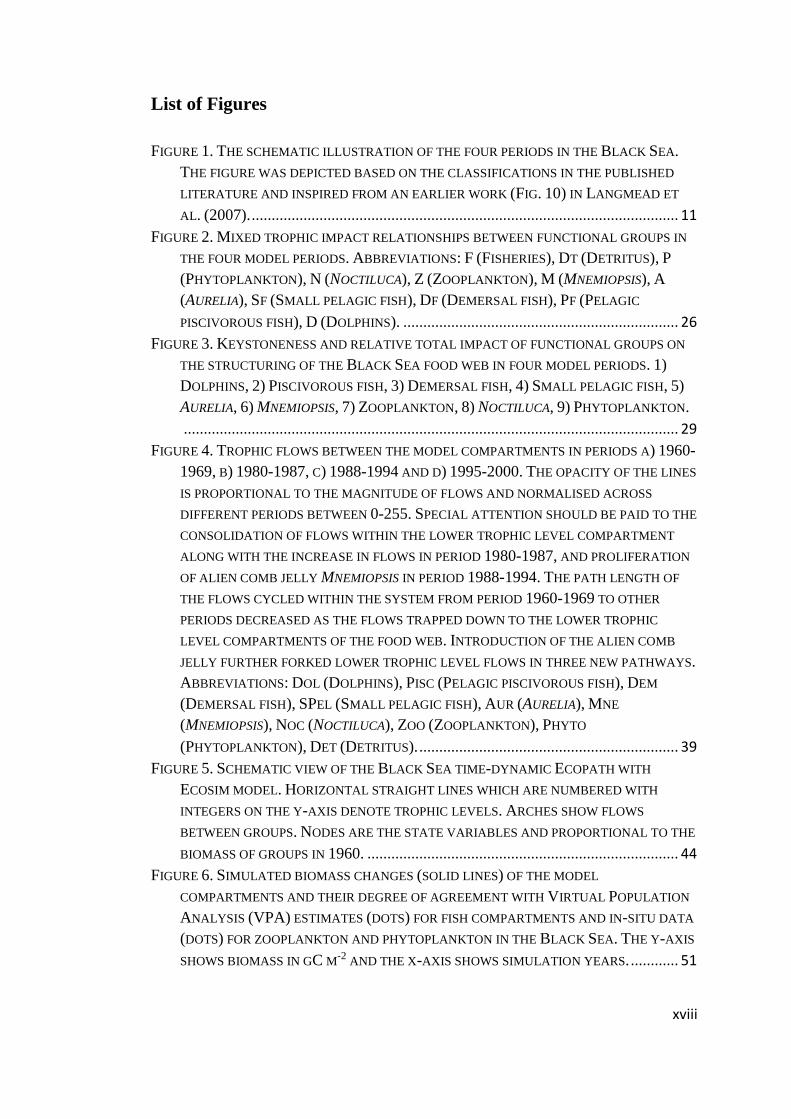
List of Figures
FIGURE 1. THE SCHEMATIC ILLUSTRATION OF THE FOUR PERIODS IN THE BLACK SEA.
THE FIGURE WAS DEPICTED BASED ON THE CLASSIFICATIONS IN THE PUBLISHED
LITERATURE AND INSPIRED FROM AN EARLIER WORK (FIG. 10) IN LANGMEAD ET
AL. (2007). ........................................................................................................... 11
FIGURE 2. MIXED TROPHIC IMPACT RELATIONSHIPS BETWEEN FUNCTIONAL GROUPS IN
THE FOUR MODEL PERIODS. ABBREVIATIONS: F (FISHERIES), DT (DETRITUS), P
(PHYTOPLANKTON), N (NOCTILUCA), Z (ZOOPLANKTON), M (MNEMIOPSIS), A
(AURELIA), SF (SMALL PELAGIC FISH), DF (DEMERSAL FISH), PF (PELAGIC
PISCIVOROUS FISH), D (DOLPHINS). ..................................................................... 26
FIGURE 3. KEYSTONENESS AND RELATIVE TOTAL IMPACT OF FUNCTIONAL GROUPS ON
THE STRUCTURING OF THE BLACK SEA FOOD WEB IN FOUR MODEL PERIODS. 1)
DOLPHINS, 2) PISCIVOROUS FISH, 3) DEMERSAL FISH, 4) SMALL PELAGIC FISH, 5)
AURELIA, 6) MNEMIOPSIS, 7) ZOOPLANKTON, 8) NOCTILUCA, 9) PHYTOPLANKTON.
............................................................................................................................ 29
FIGURE 4. TROPHIC FLOWS BETWEEN THE MODEL COMPARTMENTS IN PERIODS A) 1960-
1969, B) 1980-1987, C) 1988-1994 AND D) 1995-2000. THE OPACITY OF THE LINES
IS PROPORTIONAL TO THE MAGNITUDE OF FLOWS AND NORMALISED ACROSS
DIFFERENT PERIODS BETWEEN 0-255. SPECIAL ATTENTION SHOULD BE PAID TO THE
CONSOLIDATION OF FLOWS WITHIN THE LOWER TROPHIC LEVEL COMPARTMENT
ALONG WITH THE INCREASE IN FLOWS IN PERIOD 1980-1987, AND PROLIFERATION
OF ALIEN COMB JELLY MNEMIOPSIS IN PERIOD 1988-1994. THE PATH LENGTH OF
THE FLOWS CYCLED WITHIN THE SYSTEM FROM PERIOD 1960-1969 TO OTHER
PERIODS DECREASED AS THE FLOWS TRAPPED DOWN TO THE LOWER TROPHIC
LEVEL COMPARTMENTS OF THE FOOD WEB. INTRODUCTION OF THE ALIEN COMB
JELLY FURTHER FORKED LOWER TROPHIC LEVEL FLOWS IN THREE NEW PATHWAYS.
ABBREVIATIONS: DOL (DOLPHINS), PISC (PELAGIC PISCIVOROUS FISH), DEM
(DEMERSAL FISH), SPEL (SMALL PELAGIC FISH), AUR (AURELIA), MNE
(MNEMIOPSIS), NOC (NOCTILUCA), ZOO (ZOOPLANKTON), PHYTO
(PHYTOPLANKTON), DET (DETRITUS). ................................................................. 39
FIGURE 5. SCHEMATIC VIEW OF THE BLACK SEA TIME-DYNAMIC ECOPATH WITH
ECOSIM MODEL. HORIZONTAL STRAIGHT LINES WHICH ARE NUMBERED WITH
INTEGERS ON THE Y-AXIS DENOTE TROPHIC LEVELS. ARCHES SHOW FLOWS
BETWEEN GROUPS. NODES ARE THE STATE VARIABLES AND PROPORTIONAL TO THE
BIOMASS OF GROUPS IN 1960. .............................................................................. 44
FIGURE 6. SIMULATED BIOMASS CHANGES (SOLID LINES) OF THE MODEL
COMPARTMENTS AND THEIR DEGREE OF AGREEMENT WITH VIRTUAL POPULATION
ANALYSIS (VPA) ESTIMATES (DOTS) FOR FISH COMPARTMENTS AND IN-SITU DATA
(DOTS) FOR ZOOPLANKTON AND PHYTOPLANKTON IN THE BLACK SEA. THE Y-AXIS
SHOWS BIOMASS IN GC M-2
AND THE X-AXIS SHOWS SIMULATION YEARS. ............ 51
xix
FIGURE 7. SIMULATED YIELD CHANGES (SOLID LINES) OF THE MODEL COMPARTMENTS
AND THEIR DEGREE OF AGREEMENT WITH STATISTICAL CATCH DATA (DOTS) IN THE
BLACK SEA. THE Y-AXIS SHOWS BIOMASS IN GC M-2
AND THE X-AXIS SHOWS
SIMULATION YEARS.............................................................................................. 52
FIGURE 8. THE TIME-DYNAMIC CHANGES IN THE INDICATORS (DOTS) AND THE REGIMES
DETECTED (LINES) BY THE STARS ALGORITHM. ABBREVIATIONS ARE AS
FOLLOWS: TST (TOTAL SYSTEM THROUGHPUT), FCI (FINN’S CYCLING INDEX),
%PPR (RELATIVE PRIMARY PRODUCTION REQUIRED TO SUPPORT CATCHES),
MTLC (MEAN TROPHIC LEVEL OF CATCH), AND FIB (FISHING IN BALANCE). THE
TST, PRIMARY PRODUCTION, CATCH, AND BIOMASS PROPERTIES ARE IN GC M-2
Y-1.
FCI IS PERCENT OF TST. ASCENDENCY, OVERHEAD AND %PPR ARE IN
PERCENTAGES. OTHER INDICATORS ARE UNITLESS. THE X-AXIS DENOTES
SIMULATION YEARS.............................................................................................. 56
FIGURE 9. LARGE FISH BY WEIGHT SIMULATED BY THE TIME-DYNAMIC MODEL. DOTS
REPRESENT THE MODEL SIMULATION AND LINE REPRESENTS THE REGIMES
DETECTED BY THE STARS ANALYSIS. ................................................................. 57
FIGURE 10. THE TIME-DYNAMIC CHANGES IN THE RATIOS (DOTS) AND THE REGIMES
DETECTED (LINES) BY THE STARS ALGORITHM. THE X-AXIS DENOTES
SIMULATION YEARS.............................................................................................. 58
FIGURE 11. THE RATIO OF HETEROTROPHIC DINOFLAGELLATE NOCTILUCA BIOMASS TO
THE SUM OF NOCTILUCA AND PHYTOPLANKTON BIOMASS. DOTS REPRESENT THE
MODEL SIMULATION AND LINE REPRESENTS THE REGIMES DETECTED BY THE
STARS ANALYSIS. .............................................................................................. 59
FIGURE 12. PRIMARY PRODUCTION REQUIRED (PPR) TO SUSTAIN FISHERIES CATCHES.
............................................................................................................................ 61
FIGURE 13. FLOW BETWEEN VULNERABLE (𝑽𝒊) AND INVULNERABLE PREY BIOMASS
(𝑩𝒊 − 𝑽𝒊) IN ECOSIM. 𝒗 IS THE EXCHANGE RATE BETWEEN VULNERABLE AND
INVULNERABLE COMPARTMENTS. 𝒂𝒊𝒋 IS THE SEARCH RATE OF THE PREDATOR J
FOR PREY I (FROM CHRISTENSEN ET AL., 2005). ................................................... 65
FIGURE 14. THE RESIDUALS OF THE SIMULATED BIOMASSES OF THE STATE VARIABLES
SHOWING THE DEGREE OF MISFIT BETWEEN EWE 6 AND EWE-FORTRAN MODEL
SIMULATION OUTPUTS FOR THE GENERIC 37 MODEL. ........................................... 72
FIGURE 15. COUPLED BLACK SEA MODEL SCHEME. LIGHT-GREY BOXES REPRESENT
BIMS-ECO MODEL COMPARTMENTS AND ORANGE BOXES REPRESENT EWE
BLACK SEA MODEL COMPARTMENTS. ARROWS INDICATE FLOWS IN TERMS OF
PREY-PREDATOR INTERACTIONS. ......................................................................... 75
FIGURE 16. BIMS-ECO LOWER TROPHIC LEVEL MODEL STRUCTURE (FROM OGUZ ET
AL., 2001). ........................................................................................................... 76
FIGURE 17. PD RUN: SIMULATED BIOMASS CHANGES (SOLID LINES) OF THE MODEL
COMPARTMENTS AND THEIR DEGREE OF AGREEMENT WITH VIRTUAL POPULATION
ANALYSIS (VPA) ESTIMATES (DOTS) FOR FISH COMPARTMENTS. THE Y-AXIS
SHOWS BIOMASS IN GC M-2
AND THE X-AXIS SHOWS SIMULATION YEARS. ............ 81
xx
FIGURE 18. PD RUN: SIMULATED YIELD CHANGES (SOLID LINES) OF THE MODEL
COMPARTMENTS AND THEIR DEGREE OF AGREEMENT WITH STATISTICAL CATCH
DATA (DOTS) IN THE BLACK SEA. THE Y-AXIS SHOWS BIOMASS IN GC M-2
AND THE
X-AXIS SHOWS SIMULATION YEARS. ..................................................................... 82
FIGURE 19. ANNUAL MEAN TIME SERIES OF DEPTH-INTEGRATED AND BASIN-AVERAGED
NET PRIMARY PRODUCTION OF PD (LEFT) AND A1B (RIGHT) SCENARIOS IN THE
BLACK SEA (FROM CANNABY ET AL., 2012). ....................................................... 83
FIGURE 20. ANNUAL MEAN TIME SERIES OF DEPTH-INTEGRATED AND BASIN-AVERAGED
PHYTOPLANKTON BIOMASS OF PD (LEFT) AND A1B (RIGHT) SCENARIOS IN THE
BLACK SEA (FROM CANNABY ET AL., 2012). ....................................................... 84
FIGURE 21. ANNUAL MEAN TIME SERIES OF DEPTH-INTEGRATED AND BASIN-AVERAGED
ZOOPLANKTON BIOMASS OF PD (LEFT) AND A1B (RIGHT) SCENARIOS IN THE
BLACK SEA (FROM CANNABY ET AL., 2012). ....................................................... 84
FIGURE 22. ANNUAL MEAN TIME SERIES OF DEPTH-INTEGRATED AND BASIN-AVERAGED
AURELIA BIOMASS OF PD (LEFT) AND A1B (RIGHT) SCENARIOS IN THE BLACK SEA
(FROM CANNABY ET AL., 2012). .......................................................................... 85
FIGURE 23. ANNUAL MEAN TIME SERIES OF DEPTH-INTEGRATED AND BASIN-AVERAGED
MNEMIOPSIS BIOMASS OF PD (LEFT) AND A1B (RIGHT) SCENARIOS IN THE BLACK
SEA (FROM CANNABY ET AL., 2012). ................................................................... 86
FIGURE 24. BIOMASS DISTRIBUTIONS OF FISH AND DOLPHINS GROUPS IN PD (LEFT) AND
A1B (RIGHT) SIMULATIONS. THE Y-AXIS SHOWS BIOMASS IN GC M-2
AND THE X-
AXIS SHOWS SIMULATION YEARS. ........................................................................ 88
FIGURE 25. FRACTIONAL CHANGE PREDICTED FOR FISH AND DOLPHIN GROUPS IN A1B
(2080-2099) SCENARIO RELATIVE TO THE PD (1980-1999) SCENARIO. ............... 89
FIGURE 26. THE TIME-DYNAMIC CHANGES IN THE INDICATORS (DOTS) AND THE
REGIMES DETECTED (LINES) BY THE STARS ALGORITHM. ABBREVIATIONS ARE AS
FOLLOWS: TST (TOTAL SYSTEM THROUGHPUT), FCI (FINN’S CYCLING INDEX),
%PPR (RELATIVE PRIMARY PRODUCTION REQUIRED TO SUPPORT CATCHES),
MTLC (MEAN TROPHIC LEVEL OF CATCH), AND FIB (FISHING IN BALANCE). THE
TST, PRIMARY PRODUCTION, CATCH, AND BIOMASS VALUES ARE IN GC M-2
Y-1.
FCI IS PERCENT OF TST. ASCENDENCY, OVERHEAD AND %PPR ARE IN
PERCENTAGES. OTHER INDICATORS ARE UNITLESS. THE X-AXIS DENOTES
SIMULATION YEARS.............................................................................................. 93
FIGURE 27. THE TIME-DYNAMIC CHANGES IN THE RATIOS (DOTS) AND THE REGIMES
DETECTED (LINES) BY THE STARS ALGORITHM. THE X-AXIS DENOTES THE
SIMULATION YEARS.............................................................................................. 94
FIGURE 28. SIMULATED CHANGES IN ALL FISH BIOMASS UNDER CURRENT (F), 50%
INCREASED (F + 50%) AND 50% DECREASED (F – 50%) FISHING MORTALITY
VALUES FOR THE PD SCENARIO. .......................................................................... 95
FIGURE 29. LARGE FISH BY WEIGHT IN PRESENT DAY (PD) SCENARIO FOR THREE
DIFFERENT FISHING MORTALITY REGIMES. ........................................................... 96
xxi
FIGURE 30. THE SIMULATED ANCHOVY STOCK BIOMASS PROGRESSIONS IN PD; SCEN. 1:
FMSY = 0.41; SCEN. 2: FMSY = 0.41 AND CONSTANT PRIMARY PRODUCTION (~293.6
MGC M-2
DAY-1); SCEN. 3: FMSY = 0.41 ALONG WITH NO MNEMIOPSIS AND BEROE
INTRODUCTION; AND SCEN. 4: FMSY = 0.41, CONSTANT PRIMARY PRODUCTION
(~293.6 MGC M-2
DAY-1) ALONG WITH NO MNEMIOPSIS AND BEROE INTRODUCTION,
SCEN. 5: PD ECOSYSTEM CONDITIONS BUT WITH NO MNEMIOPSIS AND BEROE
INTRODUCTION, AND SCEN 6: PD ECOSYSTEM CONDITIONS WITH CONSTANT
PRIMARY PRODUCTION (~293.6 MGC M-2
DAY-1). ................................................. 98
FIGURE 31. THE SIMULATED ANCHOVY STOCK CATCH PROGRESSIONS IN PD; SCEN. 1:
FMSY = 0.41; SCEN. 2: FMSY = 0.41 AND CONSTANT PRIMARY PRODUCTION (~293.6
MGC M-2
DAY-1); SCEN. 3: FMSY = 0.41 ALONG WITH NO MNEMIOPSIS AND BEROE
INTRODUCTION; AND SCEN. 4: FMSY = 0.41, CONSTANT PRIMARY PRODUCTION
(~293.6 MGC M-2
DAY-1) ALONG WITH NO MNEMIOPSIS AND BEROE INTRODUCTION,
SCEN. 5: PD ECOSYSTEM CONDITIONS BUT WITH NO MNEMIOPSIS AND BEROE
INTRODUCTION, AND SCEN 6: PD ECOSYSTEM CONDITIONS WITH CONSTANT
PRIMARY PRODUCTION (~293.6 MGC M-2
DAY-1). ................................................. 99

1
1. CHAPTER: Thesis introduction
This thesis work was dedicated to explore and discover the historical and
contemporary ecosystem characteristics of the Black Sea, the structure and functioning
of its food web and its interactions with anthropogenic and climatological factors. The
fundamental approach used to achieve the objectives was based on ecological
modelling practices using three different schemes; i) a mass-balance modelling
scheme, ii) a time-dynamic modelling scheme, and iii) a coupled end-to-end lower
trophic level (LTL) and higher-trophic-level (HTL) modelling scheme. For this
purpose, the widely adopted Ecopath with Ecosim (hereinafter EwE, Christensen,
2005) model was used in each scheme. The mass-balance modelling scheme
incorporated the Black Sea ecosystem’s food web structure over the second half of the
20th century using Ecopath snapshots of four discrete periods of the Black Sea between
1960-1969, 1980-1987, 1988-1994, and 1995-2000 by averaging conditions of the
food web structure of the respective periods over its time frame. The time-dynamic
modelling scheme took this discrete mass-balance Ecopath modelling approach onto a
continuous Ecosim simulation between 1960 and 1999 and investigated the dynamics
of the food web components under changing environmental and anthropogenic
conditions. Finally, this time-dynamic model of the Black Sea was coupled with a
detailed biogeochemical model of the Black Sea; BIMS-ECO, in order to investigate
the future progressions of the ecosystem under projected future climate scenarios.
This work utilised a broad set of ecological indicators in order to bisect the
Black Sea’s environmental evolution (status over time) and tried to address and
develop options for delivering ecosystem-based management practices which fell
within the scope of the Marine Strategy Framework Directive (hereinafter MSFD,
2008/56/European Commission). MSFD is a framework that requires good
environmental status (GES) to be achieved in all European Regional Seas by the year
2020 via implementing necessary management and research policies. The Black Sea
is considered as one of the European regional seas due to the fact that some of its
riparian countries are EU members, i.e. Bulgaria and Romania, or, like Turkey, is a

2
candidate to become a full member. Therefore, it is of utmost benefit to Turkey to aim
GES not only in the Black Sea but also in all of its national seas.
For the purpose of reaching GES, the current status of the marine ecosystems
should be quantitatively documented in order to determine how far the status of any
given sea ecosystem is away from reaching GES. Further, GES itself should be
quantitatively identified so as to provide knowledge about what it is to aim in order to
achieve GES in a given marine ecosystem. For this purpose, Cardoso et al. (2010)
elaborated the eleven MSFD descriptors to provide quantitative criteria to assess the
status of marine ecosystems and defined that in what condition the marine ecosystems
could be considered in GES. They provided definitions to eleven descriptors made up
of several indicators to delineate the GES and these descriptors were as follows:
1. Biological diversity
2. Non-indigenous species
3. Commercially exploited fish and shellfish populations
4. Food webs
5. Eutrophication
6. Sea floor integrity
7. Hydrographical conditions
8. Contaminants
9. Food safety
10. Litter
11. Energy and noise
In relation to the modelling approach adopted in this study, the analyses and
the methodology used provided quantitative indicators to five of these eleven
descriptors, namely i) biological diversity, ii) non-indigenous species, iii)
commercially exploited fish and shellfish populations, iv) food webs and v)
eutrophication. These five descriptors and the related indicators used in this thesis’
study were as follows:
1. Biological diversity: This descriptor was defined in Cardoso et al. (2010)
in accordance with the Convention on Biological Diversity (United
Nations, 1992) as “the variability among living organisms from all sources

3
including, inter alia, [terrestrial,] marine [and other aquatic ecosystems]
and the ecological complexes of which they are part; this includes diversity
within species, between species and of ecosystems”. Three of its four
attributes given in Cardoso et al. (2010) and its related indicators were of
concern in this thesis study, namely; i) species state, ii) habitat/community
state, and iii) ecosystem state. In this study, the indicators used related to
these attributes and their explanations were summarised in Table 1.
Table 1. Indicators of biological diversity used in the study and their explanations.
Att
rib
ute
MS
FD
Crit
eri
a
MSFD
Indicators
Corresponding Indicators
(this study)
Explanation
Spec
ies
sta
te
Po
pu
lati
on
size
Population
biomass
Population biomass The population biomass of any given species should be
within safe biological limits so as not to drive itself to
vulnerable conditions in terms of extinction.
Po
pu
lati
on
cond
itio
n
Population
demography
Brody growth coefficient (K)
Recruitment power
Instantaneous mortalities (F,
M, Z)
Every population of any given species in an ecosystem
should be able to self-sustain by means of its
reproductive capabilities and growth performance,
both of which should not be compromised by
anthropogenic and/or natural stressors. Mortality
levels should not exceed limits so as to cause depletion
of the population in time.
Inter- and intra-
specific
interactions
Mixed Trophic Impact
(MTI)
Any particular species should not dominate the system
so as to cause negative feedbacks to other native
species. Concerning intraspecific interactions, any
given cohort in a population should not dominate so as
to cause negative feedback mechanisms that risk the
sustainability of its population (e.g. cannibalism)
Ha
bit
at/
com
mun
ity
sta
te
Co
mm
un
ity c
ondit
ion
Species
composition
mean Trophic Level of
community (mTLco),
mean Trophic Level of catch
(mTLc), Kempton’s Q
Index, Groups ratios
The composition of organisms in a given ecosystem
should be in a state so that the proportions of the
species should not adversely affect the well-being of
other species or the structure and functioning of the
ecosystem.
Community
biomass
mean Trophic Level of
community (mTLco),
Kempton’s Q, Groups ratios
The community in an environment should be made up
of natural proportions of the resident species so as not
to dominate others adversely.
Functional Traits Keystoneness Functional traits define species in terms of their
ecological roles in the ecosystem, i.e. their impact on
ecosystem functioning. Effects of diversity in
functional traits on ecosystem processes should be
evaluated (Diaz and Cabido, 2001).

4
Eco
syst
em s
tate
Eco
syst
em
stru
ctu
re
Composition and
relative
proportions of the
ecosystem
components
Community ratios The composition and proportions of the communities
that form the ecosystem should not be in negative
feedback state; i.e. inhibiting each other so as to cause
malfunction in the ecosystem by means of invading
others’ resources or habitat (e.g. Harmful Algal
Blooms - HAB).
Eco
syst
em p
roce
sses
and
funct
ion
s
Interactions
between structural
components of the
ecosystem
Mixed Trophic Impact
(MTI),
Keystoneness
This is similar to the interspecific and intraspecific
interactions on the ecosystem state.
2. Non-indigenous species (NIS): This descriptor was defined in Cardoso
et al. (2010) as “species, subspecies or lower taxa introduced outside of their
natural range (past or present) and outside of their natural dispersal
potential”. This category also included invasive alien species (IAS). IAS were
defined as “a subset of NIS which have spread, are spreading or have
demonstrated their potential to spread elsewhere, and have an adverse effect
on biological diversity, ecosystem functioning, socio-economic values and/or
human health in invaded regions” (Cardoso et al., 2010). Two of its five
attributes were of concern in this thesis study as summarised in Table 2.
Table 2. Indicators of non-indigenous used in the study and their explanations.
Att
rib
ute
MS
FD
Crit
eri
a
MSFD
Indicators
Corresponding Indicators
(this study)
Explanation
# o
f N
IS r
eco
rded
in
the
area
Red
uce
d r
isk
of
new
in
vas
ion
s
Ratio
between NIS
and other
species
Group ratios The dominancy of NIS in a given habitat makes the
ecosystem vulnerable to other invasions. Therefore, the
ratio should be within safe biological limits so as not to
dominate the system or other species in the ecosystem.

5
Env
iro
nm
enta
l im
pac
t o
f IA
S o
n
ecosy
stem
fun
ctio
nin
g
Ab
sen
ce o
r m
inim
al i
mp
act
of
IAS
adv
erse
ly a
ffec
ting
envir
on
men
tal
qual
ity
Shifts in
trophic nets,
alteration of
energy flow
and organic
matter
cycling
Cycling indicators (Finn’s
Cycling Index), Finn’s mean
path length, proportion of
flows to detritus, transfer
efficiency analysis of
energetic flows
The IAS should not reach to the extent that they will
cause leakage in the structure and functioning in the
ecosystem by means of loss of production in the food
web.
3. Commercially exploited fish and shellfish populations: This descriptor
applied to all living marine resources used for economical purposes
(Cardoso et al., 2010). The attributes used in this thesis work and its related
indicators were summarised and explained in Table 3.
Table 3. Indicators of commercial fish used in the study and their explanations.
Att
rib
ute
MS
FD
Crit
eri
a
MSFD
Indicators
Corresponding Indicators
(this study)
Explanation
Su
stai
nab
ilit
y o
f th
e ex
plo
itat
ion
Hig
h l
on
g-t
erm
yie
ld
Fishing mortality
(F), ratio of catch
to biomass
Fishing mortality (F), Ratio
of catch to biomass
The fisheries should not deplete the stocks. The
fisheries exploitation levels (F/Z) should not approach
unity in adult stocks.
Rep
rod
uct
ive
cap
acit
y
No
co
mp
rom
ise
of
rep
rodu
ctiv
e ca
pac
ity
Spawning stock
biomass
Spawning stock biomass The reproductive capacity of any given population
should not be exploited to the extent that the
populations cannot self-sustain themselves through
their natural reproductive processes.
4. Food webs: This descriptor concerned the structure and functioning in any
given marine ecosystem with respect to organic matter recycling, energy

6
transfers and roles of the components in the food webs Table 4.
Table 4. Indicators of food webs used in the study and their explanations.
Att
rib
ute
MS
FD
Crit
eri
a
MSFD
Indicators
Corresponding Indicators
(this study)
Explanation
En
erg
y f
low
s in
th
e fo
od
web
Pro
du
ctio
n o
r bio
mas
s ra
tio
s o
f co
mpo
nen
ts
Ratio of
pelagic to
demersal fish
Zooplankton
production
required to
sustain catches
Ratio of pelagic fish biomass
to demersal fish biomass
Ratio of piscivorous fish
biomass to forage fish
biomass
Ratio piscivorous fish
biomass to other fish
biomass
Primary production required
(PPR) to sustain catches
The production in the food web should not be
selectively exported by fisheries in exceeding levels so
as to change the natural proportions of the native
populations in the ecosystem to cause diversions or
leakage in the flows of the food web.
Tro
phic
rel
atio
nsh
ips
secu
ring
lo
ng
-ter
m
via
bil
ity
of
com
ponen
ts
Trophic levels
(functional
groups)
Trophic level decomposition
(energetic flow analysis)
Biomass by trophic level
The energy flows in the food web should be
sufficiently distributed across all trophic levels.
Trapping-down of energy in one of the trophic levels
may cause loss in system’s production.
Str
uct
ure
of
food
web
s
Pro
po
rtio
n o
f la
rge
fish
mai
nta
ined
Proportion of
large fish by
weight
Proportion of large fish by
weight
This is an indicator of the fishing pressure as well as
how the flows (energy, production) in the ecosystem
are shared among its components. In any given
ecosystem, the higher trophic levels should be
sufficiently represented by predatory species.
Ab
und
ance
/
dis
trib
uti
on
mai
nta
ined
Charismatic
indicator
species
Keystoneness These species indicate whether a food web in an
ecosystem is performing well, i.e. have the diversity in
the web that could be used as indicators of flows in the
ecosystem. Such species are usually marine mammals
and large fish species.

7
Groups species
targeted by
fishing and
their response
to exploitation
Fishing in Balance Index
(FiB)
Mean trophic level of catch
(mTLc)
Similar to biomass ratios of components, the trophic
levels in a food web should not be underrepresented by
means of continuous selective extraction of certain
components so as to cause overpopulation in certain
levels of the food web.
5. Eutrophication: This descriptor concerned human-introduced
eutrophication and its adverse effects in terms of damage to the ecosystem
structure and functioning Table 5.
Table 5. Indicators of eutrophication used in the study and their explanations.
Att
rib
ut
e
MS
FD
Crit
eri
a
MSFD
Indicators
Corresponding Indicators
(this study)
Explanation
Ph
yto
pla
nkto
n b
iom
ass
Incr
ease
/ d
ecre
ase
Opportunistic
species
Ratio of opportunistic r-
selected species to K-
selected species
Used as a proxy for deterioration of primary
production to cause adverse effects on the higher
trophic level communities.
All of the above attributes and related criteria and indicators were discussed in
the forthcoming chapters. The chapters 2, 3 and 5 examined the ecosystem structure
and functioning with increasing level of complexity. The second chapter was
dedicated to analyse and assess the ecosystem structure and functioning of the
Black Sea ecosystem utilising mass-balance snapshots of the discrete phases it had
undergone in the second half of the twentieth century through a set of
synthetically calculated ecological indicators of energetic flows, catches and
biomasses.
The third chapter elaborated the analyses given in the second chapter
using a dynamic EwE model of the Black Sea ecosystem between 1960 and 2000,
and examined the time-dynamic changes of a broader set of ecological indicators
in search for different regimes prevailed during the changes the Black Sea had

8
undergone and the causes behind the shifts of the detected regimes as well as the
dynamic evolution of the ecological indicators and what they did represent
throughout the simulation period in terms of functioning of the Black Sea
ecosystem.
The fourth chapter dealt with technical difficulties of coupling EwE
models with biogeochemical models that were mostly written in FORTRAN and,
hence, presented the FORTRAN transcription of the EwE model in order to make
this powerful modelling tool ready for coupling with such models.
The fifth chapter expanded the time-dynamic model of the Black Sea used
in the third chapter so as to include a sophisticated lower trophic level
representation by coupling with a biogeochemical model of the Black Sea in order
to investigate the impacts of the changes in the lower trophic level compartments
under climatologic and anthropogenic drivers on the higher trophic level
assemblages of the Black Sea between 1980 and 1999. This chapter also
elaborated the investigation of the ecological indicators used in the previous
chapters in more detail in order to describe the impacts of inclusion of a refined
representation of the lower trophic level compartment on the higher trophic level
organisms and aimed to explain the changes in the Black Sea from a more detailed
perspective. It also aimed to answer the question of under which conditions and
ecosystem-based management practices the Black Sea ecosystem could be
improved towards its GES. Further, this chapter included a forecast simulation
for the Intergovernmental Panel on Climate Change (IPCC) A1B carbon
emission scenario in order to investigate the impacts of predicted climatologic
changes between 2080 and 2099 on the Black Sea ecosystem. Finally in the sixth
chapter, a summary was given in relation to the above mentioned MSFD
indicators by making a detailed diagnosis of the Black Sea ecosystem structure
and functioning from the perspective of its GES.

9
2. CHAPTER: An indicator-based evaluation of the Black Sea
food web dynamics during 1960 – 2000 using mass-balance
HTL models
2.1. Introduction
The Black Sea ecosystem had been through significant trophic transformations
over the second half of the 20th century (Oguz and Gilbert, 2007). The history of these
changes could be classified into four distinctive periods; 1) the 1960s - pre-eutrophication,
2) 1980-1987 - representing intense eutrophication, 3) 1988-1994 - the infamous
Mnemiopsis leidyi (Agassiz, 1865) – anchovy shift, and 4) 1995-2000 - signifying the post-
eutrophication phase (Figure 1). The principal reasons for these transformations have long
been debated (Zaitsev, 1992; Shiganova, 1998; Kovalev and Piontkovski, 1998; Kovalev
et al., 1998; Kideys et al., 2000; Oguz et al., 2003; Yunev et al., 2002, 2007; Bilio and
Nierman, 2004; Oguz and Gilbert, 2007; McQuatters-Gollop et al., 2008). Whilst primarily
focusing on the anchovy - Mnemiopsis shift in 1989 (Kideys, 2002), studies sought
answers to enhance comprehension of the mechanisms underlying the observed changes
(Berdnikov, 1999; Daskalov, 2002; Gucu, 2002; Daskalov et al., 2007; Oguz, 2007; Oguz
et al., 2008a, b; Llope et al., 2011). The roles of trophic cascades through overfishing
(Daskalov, 2002; Gucu, 2002), Mnemiopsis leidyi (hereafter referred to as Mnemiopsis)
predation on anchovy eggs and larvae (Lebedeva and Shushkina, 1994; Shiganova and
Bulgakova, 2000; Kideys, 2002) and the combination of bottom-up and top-down controls
(Bilio and Nierman, 2004; Oguz, 2007; Oguz et al., 2008a, b) were all suggested as
significant factors catalysing these changes.
The pre-eutrophication phase of the 1960s characterised a healthy mesotrophic
ecosystem with primary production values between 100-200 mgC m-2 y-1 (Oguz et al.,
2012). Relatively rich biological diversity of the 1960s’ Black Sea comprised fishes from
large demersal fish species such as turbot (Psetta maeotica, Pallas, 1814), Black Sea
striped mullet (Mullus barbatus ponticus, Essipov, 1927), spiny dogfish (Squalus
acanthias, Linnaeus, 1758), and Black Sea whiting (Merlangius merlangus euxinus,
Nordmann, 1840) to piscivorous pelagic fish; Atlantic bonito (Sarda sarda; Bloch,

10
1973), bluefish (Pomatomus saltator; Linnaeus, 1776), and Atlantic mackerel (Scomber
scombrus; Linnaeus, 1758) as well as small pelagic fish; predominantly the Black Sea
anchovy (Engraulis encrasicolus ponticus; Alexandrov, 1927), Black Sea horse
mackerel (Trachurus mediterraneaus ponticus; Aleev, 1956), and Black Sea sprat
(Sprattus sprattus phalaericus; Risso, 1827). Three cetacean species; the Black Sea
common dolphin (Delphinus delphis spp. ponticus; Barabash-Nikiforov, 1935), the
Black Sea bottlenose dolphin (Tursiops truncatus spp. ponticus; Barabasch, 1940), and
the Black Sea harbour porpoise (Phocoena phocoena spp. relicta; Abel, 1905)
constituted the top predators of the system. During the subsequent two decades, the stocks
of both pelagic piscivorous fishes and marine mammals had been overexploited and
further, primary and secondary pelagic production increased excessively due to nutrient
enrichment from the rivers discharging mainly into the northwestern shelf of the Black
Sea. The small pelagic fish species and the moon jelly; Aurelia aurita (Linnaeus, 1758),
thus became dominant in the ecosystem. The benthic flora and fauna deteriorated to a great
extent due to the frequent hypoxia events on the shelf waters (Zaitsev, 1992; Zaitsev and
Mamaev, 1997; Mee, 2006). Simultaneously, the Turkish fishing fleet developed
enormously in size and technology (Gucu, 2002) and the fisheries yield attained 700 kt, a
significant proportion (~500 kt) of which consisted of anchovy. In 1989, the non-
indigenous comb jelly species Mnemiopsis leidyi (Agassiz, 1865), which was introduced
to the Black Sea ecosystem in the early 1980s via the ballast waters of shipping vessels,
flourished both in abundance and biomass. This same year also coincided with the collapse
of the total Turkish fisheries yield from an average of 700 kt during the early 1980s to only
150 kt in 1989 (Oguz, 2007). Subsequently, the Turkish fishery yield recovered to about
300 ± 100 kt whereas it remained at very low levels throughout the rest of the Black Sea
(Oguz et al., 2012). During this recuperation period, blooms of Mnemiopsis were
suppressed naturally due to the appearance of another non-indigenous gelatinous species;
Beroe ovata (Mayer, 1912), an inherent Mnemiopsis predator. By the end of the 1990s,
the Black Sea ecosystem as a whole was characterised by moderate primary (200-400 mgC
m-2 y-1, Oguz et al. (2012)) and secondary productivity (Mee, 2006; McQuatters-Gallop,
2008) although the ecosystem of the northwestern shelf and western coastal waters were
still far from recovery and rehabilitation (Oguz and Velikova, 2010).

11
Figure 1. The schematic illustration of the four periods in the Black Sea. The figure
was depicted based on the classifications in the published literature and inspired from
an earlier work (Fig. 10) in Langmead et al. (2007).
In order to investigate the aforementioned changes and the underlying
mechanisms, the various aspects of the functioning of the Black Sea lower trophic
food web were studied in terms of aggregated biogeochemical models (e.g. Oguz and
Salihoglu, 2000; Oguz et al., 2001, 2008b; Oguz and Merico, 2006; Lancelot et al.,
2002; Gregoire and Lacroix, 2003; Gregoire and Friedrich, 2004; Gregoire et al.,
2004, 2008; Gregoire and Soetaert, 2010; Tsiaras et al., 2008; Staneva et al., 2010; He
et al., 2012). Further, mass-balance models of different complexities were also
invoked by Gucu (2002), Daskalov (2002), and Orek (2000). Gucu (2002) focused on
the second half of the 1980s when examining the role of increased fishing pressure on
the collapse of anchovy stocks, whereas Daskalov (2002) adopted a broader time
frame starting from the pre-eutrophication period and pointed out that trophic cascade
12
initiated by overfishing played a leading role on the ecosystem changes. However,
both of these studies lacked the quantification and insight of ecosystem characteristics
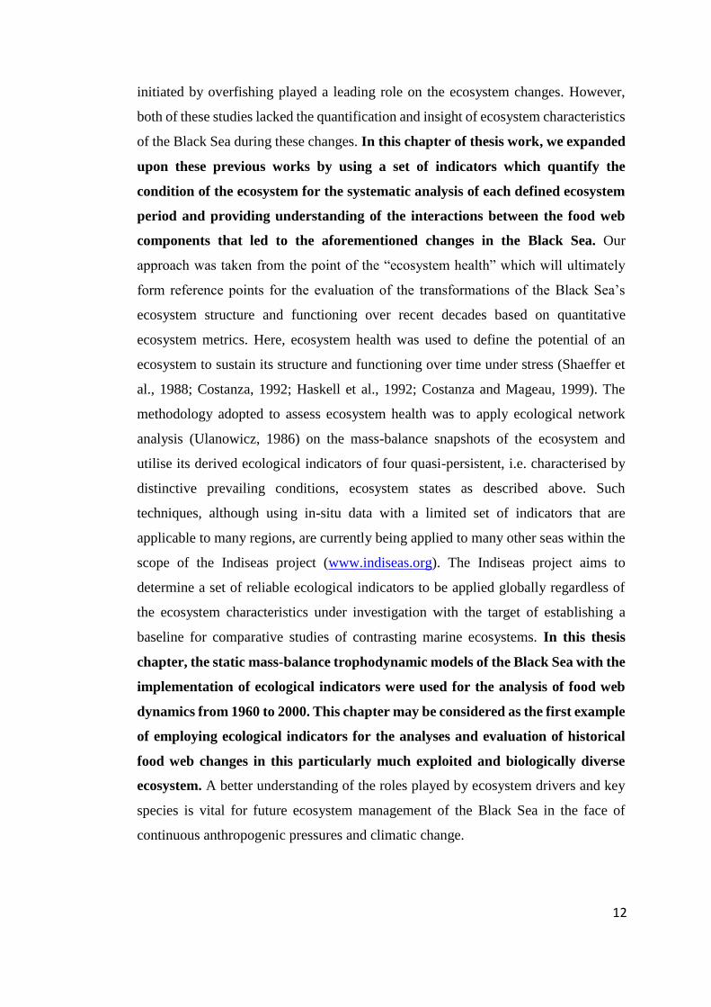
of the Black Sea during these changes. In this chapter of thesis work, we expanded
upon these previous works by using a set of indicators which quantify the
condition of the ecosystem for the systematic analysis of each defined ecosystem
period and providing understanding of the interactions between the food web
components that led to the aforementioned changes in the Black Sea. Our
approach was taken from the point of the “ecosystem health” which will ultimately
form reference points for the evaluation of the transformations of the Black Sea’s
ecosystem structure and functioning over recent decades based on quantitative
ecosystem metrics. Here, ecosystem health was used to define the potential of an
ecosystem to sustain its structure and functioning over time under stress (Shaeffer et
al., 1988; Costanza, 1992; Haskell et al., 1992; Costanza and Mageau, 1999). The
methodology adopted to assess ecosystem health was to apply ecological network
analysis (Ulanowicz, 1986) on the mass-balance snapshots of the ecosystem and
utilise its derived ecological indicators of four quasi-persistent, i.e. characterised by
distinctive prevailing conditions, ecosystem states as described above. Such
techniques, although using in-situ data with a limited set of indicators that are
applicable to many regions, are currently being applied to many other seas within the
scope of the Indiseas project (www.indiseas.org). The Indiseas project aims to
determine a set of reliable ecological indicators to be applied globally regardless of
the ecosystem characteristics under investigation with the target of establishing a
baseline for comparative studies of contrasting marine ecosystems. In this thesis
chapter, the static mass-balance trophodynamic models of the Black Sea with the
implementation of ecological indicators were used for the analysis of food web
dynamics from 1960 to 2000. This chapter may be considered as the first example
of employing ecological indicators for the analyses and evaluation of historical
food web changes in this particularly much exploited and biologically diverse
ecosystem. A better understanding of the roles played by ecosystem drivers and key
species is vital for future ecosystem management of the Black Sea in the face of
continuous anthropogenic pressures and climatic change.

13
2.2. Materials and Methods
The static mass-balance modelling of the food web was implemented by
developing an Ecopath (Christensen et al., 2005) food web model for each ecosystem
period (Figure 1). The Ecopath models of the Black Sea were built to represent the
general food web structure of the inner Black Sea basin, avoiding the extremely
variable conditions of the Northwestern Shelf (NWS). The model covered an area of
150 000 km2 where fisheries operated intensively (Oguz et al., 2008a) in the vicinity
of the exclusive economic zones (EEZs) of the six riparian countries. The geographical
representation of the model did not include depths greater than 150 m in the open Black
Sea where anoxia prevails.
2.2.1. The Model Setup
Four mass-balance Ecopath models were set up to represent the four distinctive
periods of the Black Sea ecosystem as described in the previous section. Ecopath
comprises a series of linear equations that define a mass-balance state of the food web
in the form of functional groups (each representing a species or groups of species)
linked by trophic interactions. The functional groups are regulated by gains
(consumption, immigration) and losses (mortality, emigration), and are linked to each
other by predator-prey relationships. Fisheries extract biomass from the targeted and
by-catch groups. Each linear equation describes flows of mass into and out of discrete
biomass pools of the form
𝐵𝑖 ∗ (𝑃
𝐵)𝑖−∑𝐵𝑗
𝑛
𝑗=1
∗ (𝑄
𝐵)𝑗∗ 𝐷𝐶𝑗𝑖 − 𝐵𝑖 ∗ (
𝑃
𝐵)𝑖∗ (1 − 𝐸𝐸𝑖) − 𝑌𝑖 − 𝐸𝑖 − 𝐵𝐴𝑖 = 0 (1)
where for each functional group i, B stands for biomass, (P/B)i stands for the
production to biomass ratio, (Q/B)j stands for the consumption to biomass ratio of
predator j, DCji is the fraction of prey i in the average diet of predator j, Y is the

14
landings, E is net migration rate, BA is the biomass accumulation rate, and EE is the
proportion of the production utilised in the system (Christensen et al., 2005). EE must
be less than or equal to unity under the assumption of mass-balance conservation. E
and BA values were assumed to be zero for all groups. Typically, three of B, (P/B),
(Q/B) or (P/Q) and EE parameters and diet composition are defined as input for each
functional group and the values of remaining parameters are estimated by the Ecopath
mass-balance algorithm. Ecopath software computes mass-balance by solving the
system of equations for the unknown parameters of all groups. A balanced model,
however, might not be obtained at the first parameterisation, thus it may require
iterative adjusments to the input values (usually the diet composition) following the
guidelines given by Christensen et al. (2005).
The model set-up in this investigation presented a simplified representation of
the pelagic food web structure using ten functional groups (Table 6); five of which
were the guilds of ecologically similar species, namely dolphins, pelagic piscivorous
fish, demersal fish, small pelagic fish, zooplankton and phytoplankton, whilst the other
three groups were individual species; the comb jelly Mnemiopsis, the moon jelly
Aurelia aurita (hereafter referred to as Aurelia) and the heterotrophic dinoflagellate
Noctiluca scintillans (Ehrenberg, 1834) (hereafter referred to as Noctiluca). These
organisms were represented by exclusive groups since they played specific roles (r-
selected behaviour; Pianka, 1970) in ecosystem functioning and were important
indicators of ecosystem changes during the specified periods. Since the aim of this
chapter was to investigate the changes in ecosystem structure of the Black Sea and not
the interactions amongst different types of fisheries, fisheries were collectively
represented although the Black Sea industrial fisheries included mainly three gears;
trawling, gill-netting and seining. Thus, a single fleet was considered in the model, and
fisheries yields by species were pooled to ensure correctly aggregated catches for each
functional group. For each modelled state of the Black Sea, an average annual catch
value was calculated from the data for the period investigated. The average value was
then divided by the total area of the fishing grounds (150 000 km2; Oguz et al., 2008a)
to obtain the yield per unit of fishing area.

15
Table 6. Trophic groups and main species included in the model setup.
Groups Main Species
Dolphins
Black Sea common dolphin
Black Sea bottlenose dolphin
Black Sea harbour porpoise
Pelagic Piscivorous
Fish
Bluefish
Atlantic bonito
Atlantic mackerel
Demersal
Fish
Black Sea whiting
Black Sea turbot
Black Sea striped mullet
Small Pelagic Fish
Black Sea anchovy
Black Sea sprat
Black Sea horse mackerel
Aurelia Aurelia aurita
Mnemiopsis Mnemiopsis leidyi
Noctiluca Noctiluca scintillans
Zooplankton Mesozooplankton
Microzooplankton
Phytoplankton Diatoms
Dinoflagellates
Detritus POM + Detritus
Each given ecosystem state was described by key parameters and input data
for each functional group such as biomass per unit area, rates of production and
consumption, diet composition, and fishery losses. The units were in gC m-2 year-1 for
quantities and year-1 for rates. Models that include jellyfish organisms are prone to bias
considering that the significant portion of the wet weight of these organisms are of
water. Hence, in such cases, carbon weight is the preferred currency (Pauly et al.,
2009). Because our model set-up included gelatinuous organisms as important
components of the food web, carbon weight was used as the model currency.
Considering that the catch statistics and in-situ data available in the literature were in
tons and grams wet weight per square meter respectively, the values were converted
into grams carbon per square meter using conversion factors specific to the concerning
group as listed in Table 7.

16
Table 7. Multipliers used to convert biomass and catch values from grams wet
weight into grams carbon.
Group Conversion Multiplier
(grams wet weight to grams
carbon)
Reference
Phytoplankton 0.1 O’Reilly and Dow (2006)
Zooplankton 0.08 Dow, O’Reilly and Green
(2006), Weslawski and
Legezynska (1998)
Noctiluca 0.08 Dow, O’Reilly and Green
(2006)
Aurelia 0.002 Oguz et al. (2001)
Mnemiopsis 0.001 Oguz et al. (2001)
Fish groups 0.11 Oguz et al. (2008a)
On the basis of data availability, the biomass values for dolphins and pelagic
piscivorous fish were used as input parameters for the 1960s model set-up; whereas,
for the remaining three model set-ups the estimated EE values for these two species
groups were used as input due to the lack of biomass estimates for these organisms in
the literature corresponding to the respective model periods. The EE parameters for all
of the remaining groups were calculated by the model in all model set-ups. The fraction
of the consumption which is not assilimated was set to the Ecopath’s default value 0.2
for all groups. The fisheries yields and other input values used for the parameterisation
of the four Ecopath models were summarised in Table 8. The input data were derived
from the literature and previously published mass-balance modelling studies
concerning the Black Sea and used with slight rounding modifications. However, the
input P/B and Q/B parameters for Mnemiopsis were not taken from elsewhere but
assumed to be identical to Aurelia’s. Further, since the input parameters inherited from
previously published models composed of more functional groups (e.g.
microzooplankton and mesozooplankton in Daskalov (2002)) compared to the model
set-up used in this study (e.g. zooplankton), the weighted average values of the input
parameters for such groups were computed and used in the four mass-balance models.
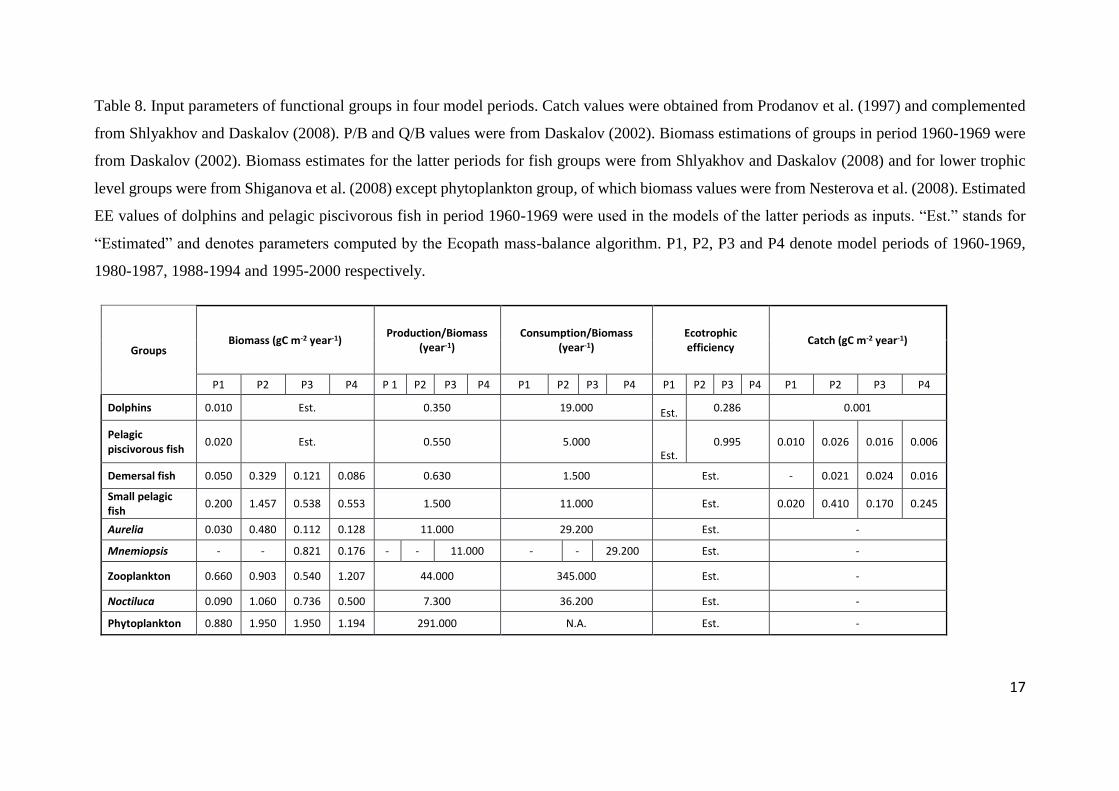
17
Table 8. Input parameters of functional groups in four model periods. Catch values were obtained from Prodanov et al. (1997) and complemented
from Shlyakhov and Daskalov (2008). P/B and Q/B values were from Daskalov (2002). Biomass estimations of groups in period 1960-1969 were
from Daskalov (2002). Biomass estimates for the latter periods for fish groups were from Shlyakhov and Daskalov (2008) and for lower trophic
level groups were from Shiganova et al. (2008) except phytoplankton group, of which biomass values were from Nesterova et al. (2008). Estimated
EE values of dolphins and pelagic piscivorous fish in period 1960-1969 were used in the models of the latter periods as inputs. “Est.” stands for
“Estimated” and denotes parameters computed by the Ecopath mass-balance algorithm. P1, P2, P3 and P4 denote model periods of 1960-1969,
1980-1987, 1988-1994 and 1995-2000 respectively.
Groups Biomass (gC m-2 year-1)
Production/Biomass (year-1)
Consumption/Biomass (year-1)
Ecotrophic efficiency
Catch (gC m-2 year-1)
P1 P2 P3 P4 P 1 P2 P3 P4 P1 P2 P3 P4 P1 P2 P3 P4 P1 P2 P3 P4
Dolphins 0.010 Est. 0.350 19.000 Est. 0.286 0.001
Pelagic piscivorous fish
0.020 Est. 0.550 5.000 Est.
0.995 0.010 0.026 0.016 0.006
Demersal fish 0.050 0.329 0.121 0.086 0.630 1.500 Est. - 0.021 0.024 0.016
Small pelagic fish
0.200 1.457 0.538 0.553 1.500 11.000 Est. 0.020 0.410 0.170 0.245
Aurelia 0.030 0.480 0.112 0.128 11.000 29.200 Est. -
Mnemiopsis - - 0.821 0.176 - - 11.000 - - 29.200 Est. -
Zooplankton 0.660 0.903 0.540 1.207 44.000 345.000 Est. -
Noctiluca 0.090 1.060 0.736 0.500 7.300 36.200 Est. -
Phytoplankton 0.880 1.950 1.950 1.194 291.000 N.A. Est. -

18
The diet composition matrix that incorporated the relative proportions of
predation on each group followed those from previous studies by Gucu (2002) and
Daskalov (2002) except for some specific adjustments (Table 9). The diets of small
pelagic fish and demersal fish were taken from Gucu (2002) and used without
modifications. The model of Gucu (2002) only included one jellyfish group by pooling
all the jellyfish species (Aurelia, Mnemiopsis and Pleurobrachia pileus) in the Black
Sea. Although the model set-up used in our study included distinctive groups for
Aurelia and Mnemiopsis and completely exluded Pleurobrachia, their diets were
assumed to be identical and therefore the diet composition given in Gucu (2002) for
the jellyfish group was used intact and the same for these two groups. The diet of
zooplankton group was taken from Gucu (2002) (50% phytoplankton and 50%
detritus), however, modified to include 60% phytoplankton and 40% detritus assuming
that zooplankton had more preference to graze on phytoplankton than detritus. The
diet of piscivorous fish was also inherited from Gucu (2002) (50% small pelagic fish,
10% demersal fish and 40% import) but modified to include 60% small pleagic fish
and 40% import by excluding the demersal fish group in their diet. The ommision of
demersal fish from the diet was done considering that the habitat distributions of these
two groups were quite distinct and therefore piscivorous fish group was inclined to
have more consumption on the small pelagic fish group. The diet of dolphins was taken
from Daskalov (2002) (96% small pleagic fish, 3.5% demersal fish and 0.5%
piscivorous fish), however, modified to include 90% small pelagic fish, 9.5% demersal
fish and 0.5% piscivorous fish in order to obtain mass-balance. The diet items of
Noctiluca were constructed following Oguz et al. (2001), who included its grazing on
phytoplankton, zooplankton and detritus. The relative proportions of the items in the
diet of Noctiluca were determined following the study of Umani et al. (2004).
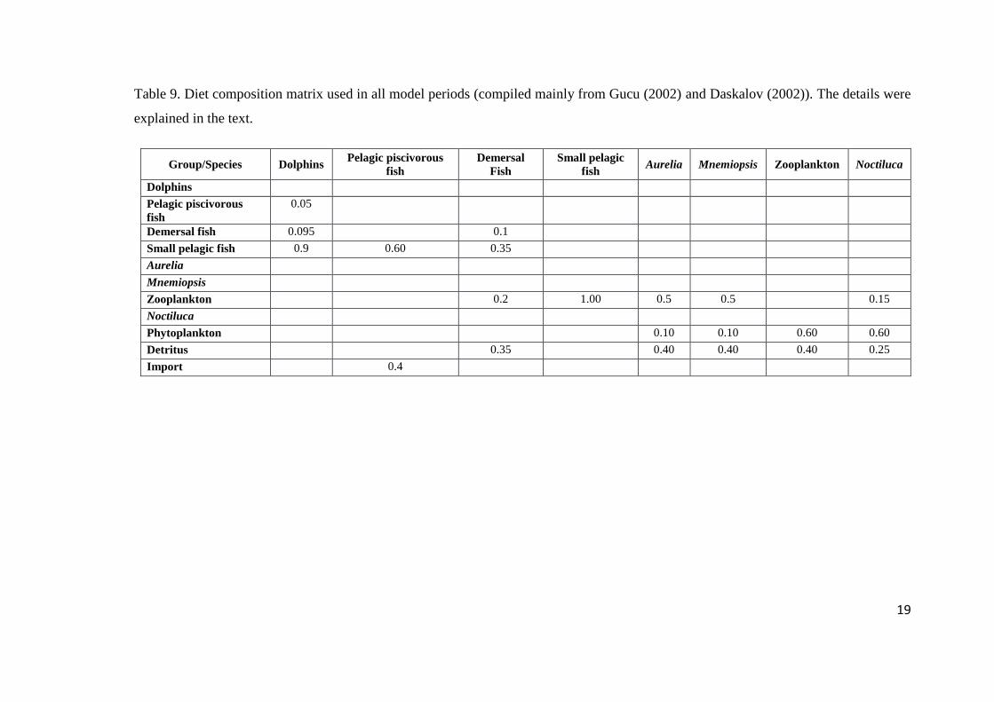
19
Table 9. Diet composition matrix used in all model periods (compiled mainly from Gucu (2002) and Daskalov (2002)). The details were
explained in the text.
Group/Species Dolphins Pelagic piscivorous
fish Demersal
Fish Small pelagic
fish Aurelia Mnemiopsis Zooplankton Noctiluca
Dolphins Pelagic piscivorous
fish 0.05
Demersal fish 0.095 0.1 Small pelagic fish 0.9 0.60 0.35 Aurelia Mnemiopsis Zooplankton 0.2 1.00 0.5 0.5 0.15
Noctiluca Phytoplankton 0.10 0.10 0.60 0.60
Detritus 0.35 0.40 0.40 0.40 0.25
Import 0.4

20
2.2.2. Ecological Indicators
The four ecosystem periods were examined by utilising several indicators
provided by the Ecopath model package using the final mass-balance biomass and
flow estimates. Mixed Trophic Impact (MTI) analysis was performed to analyse the
relative direct and indirect effects of variations within a group’s biomass on the
biomass of the other groups (Ulanowicz and Puccia, 1990). The direct impact of any
one group upon another, related to predation or fishing, might cascade to other groups
through any order of indirect interaction. MTI enables to quantify all possible direct
and indirect interactions between two groups. By defining MTI (mij) as the product of
all the impacts that group i has on group j, it is calculated as
𝑚𝑖𝑗 =∏(𝑑𝑗𝑖 − 𝑓𝑖𝑗)
𝑛
𝑖=1
(2)
where dji denotes the positive effects that i has on j and is calculated by means of the
fraction of prey i in the diet of the predator j and fij signifies the negative effects that j
has on i, calculated through the fraction of total consumption of prey i used by predator
j (Libralato et al., 2006). Mixed trophic impact values scale between -1 (strong
negative impact) and 1 (strong positive impact) and are relative measures of the
interactions between two groups. Negative values indicate an inhibiting and positive
values indicate a promoting effect between two corresponding groups.
Furthermore, keystone functional groups were determined for each model
period. Keystone groups are groups or species with relatively low biomass values
despite having an important functional role in their ecosystems (Power et al, 1996).
The keystone value of each group is calculated as
𝐾𝑆𝑖 = log[𝜀𝑖(1 − 𝑝𝑖)] (3)
where KSi is the keystoneness of group i, and pi is the ratio of the biomass of group i
(Bi) to the sum of the biomass values of all groups and is calculated as

21
𝑝𝑖 =𝐵𝑖∑𝐵𝑖
(4)
following Libralato et al. (2006).
The transfer efficiency (TE) is an index for the measure of efficiency with
which energy is transferred between adjacent trophic levels. It is calculated as the ratio
of production of a trophic level to the production of the preceding trophic level (Lalli
and Parsons, 1993). Thus, the primary producers and detritus groups are
conventionally attributed to TL I, the herbivorous fraction of flows and biomasses to
TL II, first order carnivorous flows and biomasses to TL III and second order
carnivorous flows and biomasses to TL IV. This classification allowed us to
distinguish biomasses and flows along the primary producer-based and the detritus-
based food chains. Here, transfer efficiencies were calculated by disaggregating
functional groups’ biomasses and flows at each integer trophic level (TL), and then
aggregating the results by integer TLs as defined by Lindeman (1942).
Additionally, some commonly used ecosystem indices and synthetic ecological
indicators were also employed in assessing the ecological status of the Black Sea
ecosystem for the four model periods (Table 10). These indicators were chosen
because they could easily be calculated by using simple mathematical algorithms.
They can be derived with the utilisation of basic network theory and are readily
integrated into a number of ecological network and mass-balance analyses packages
such as Ecopath.
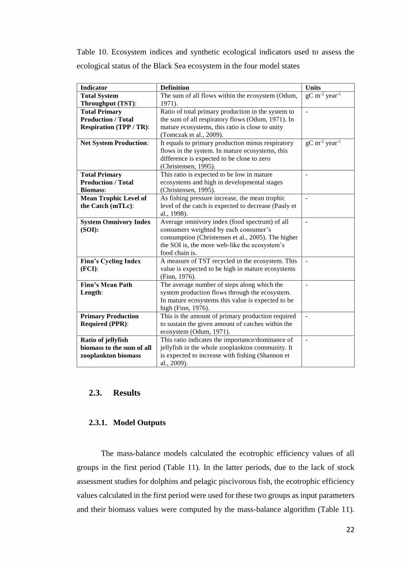
22
Table 10. Ecosystem indices and synthetic ecological indicators used to assess the
ecological status of the Black Sea ecosystem in the four model states
Indicator Definition Units
Total System
Throughput (TST):
The sum of all flows within the ecosystem (Odum,
1971).
gC m-2 year-1
Total Primary
Production / Total
Respiration (TPP / TR):
Ratio of total primary production in the system to
the sum of all respiratory flows (Odum, 1971). In
mature ecosystems, this ratio is close to unity
(Tomczak et al., 2009).
-
Net System Production: It equals to primary production minus respiratory
flows in the system. In mature ecosystems, this
difference is expected to be close to zero
(Christensen, 1995).
gC m-2 year-1
Total Primary
Production / Total
Biomass:
This ratio is expected to be low in mature
ecosystems and high in developmental stages
(Christensen, 1995).
-
Mean Trophic Level of
the Catch (mTLc):
As fishing pressure increase, the mean trophic
level of the catch is expected to decrease (Pauly et
al., 1998).
-
System Omnivory Index
(SOI):
Average omnivory index (food spectrum) of all
consumers weighted by each consumer’s
consumption (Christensen et al., 2005). The higher
the SOI is, the more web-like the ecosystem’s
food chain is.
-
Finn’s Cycling Index
(FCI):
A measure of TST recycled in the ecosystem. This
value is expected to be high in mature ecosystems
(Finn, 1976).
-
Finn’s Mean Path
Length:
The average number of steps along which the
system production flows through the ecosystem.
In mature ecosystems this value is expected to be
high (Finn, 1976).
-
Primary Production
Required (PPR):
This is the amount of primary production required
to sustain the given amount of catches within the
ecosystem (Odum, 1971).
-
Ratio of jellyfish
biomass to the sum of all
zooplankton biomass
This ratio indicates the importance/dominance of
jellyfish in the whole zooplankton community. It
is expected to increase with fishing (Shannon et
al., 2009).
-
2.3. Results
2.3.1. Model Outputs
The mass-balance models calculated the ecotrophic efficiency values of all
groups in the first period (Table 11). In the latter periods, due to the lack of stock
assessment studies for dolphins and pelagic piscivorous fish, the ecotrophic efficiency
values calculated in the first period were used for these two groups as input parameters
and their biomass values were computed by the mass-balance algorithm (Table 11).

23
For all the other functional groups, ecotrophic efficiency values were calculated by the
model for periods two, three and four. Further, respiratory flows for all functional
groups were calculated from energetic balance of the sources and sinks in each
functional compartment (Table 11) as the model product and were in compliance with
the energy budget of each state variable described in the model which assumed that
the consumption of a group was the sum of production, respiration, and unassimilated
food. The increases in respiratory flows of zooplankton and gelatinous organisms as
well as small pelagic fish from the first period to the second and third periods were
remarkable. The decrease in estimated biomass levels of piscivorous fish from the first
period to the latter periods was also pronounced and found to be in correspondence
with the explanations provided by others (Gucu, 2002; Oguz, 2007).
The primary production values calculated by the model were 256, 567, 567 and
347.5 mg C m-2 d-1 for the four periods respectively. The primary production values
were found to be marginally overestimated for the first period (100-200 mgC m-2 d-1)
and underestimated for the second and third periods (600-800 mgC m-2 d-1 for 1975-
1990) and in the last period primary production matched the literature averages (200-
400 mgC m-2 d-1) (Oguz et al., 2012, Yunev et al. 2002).

24
Table 11. Basic output parameters calculated by the Ecopath for the four modelled periods. P1, P2, P3 and P4 denote model periods of 1960-
1969, 1980-1987, 1988-1994 and 1995-2000 respectively.
Parameter / Group
Ecotrophic Efficiency Biomass (gC m-2y-1) Respiration (gC m-2y-1)
P1 P2 P3 P4 P1 P2 P3 P4 P1 P2 P3 P4
Dolphins 0.296 - 0.01 0.01 0.01 0.15 0.15 0.15 0.15
Piscivorous fish 0.995 - 0.05 0.03 0.01 0.07 0.17 0.11 0.05
Demersal fish 0.811 0.427 0.791 0.862 - 0.03 0.19 0.07 0.05
Small pelagic fish 0.924 0.413 0.618 0.603 - 1.46 10.64 3.93 4.04
Aurelia 0 - 0.37 5.93 1.38 1.58
Mnemiopsis 0 - - - 10.15 2.18
Zooplankton 0.108 0.727 0.992 0.25 - 153.1 209.50 125.30 280.0
Noctiluca 0 - 1.949 22.96 15.94 10.83
Phytoplankton 0.541 0.372 0.230 0.753 - -
Detritus 0.483 0.306 0.183 0.783 - -

25
2.3.2. Mixed Trophic Impact
The MTI analysis was performed separately for fishery and interspecies
competition among gelatinous organisms and small pelagic fish, and predation impact
of the opportunistic species Noctiluca on zooplankton and phytoplankton groups
(Figure 2). According to the analysis, fisheries incurred positive mixed trophic impacts
on demersal (0.489) and small pelagic fish (0.308) groups, whereas it sustained
negative impacts on dolphins (-0.650) and pelagic piscivorous fish (-0.645) groups for
the period 1960-1969. The positive impacts on small pelagic and demersal fish groups
were realised due to the positive indirect impacts of fisheries on these groups (i.e. the
exploitation of their predators; dolphins and pelagic piscivorous fish) exceeded the
direct negative impacts due to harvesting. Conversely, in the model period 1980-1987,
the fisheries impacts on all fish groups as well as dolphins were negative (-0.954 for
dolphins, -0.865 for piscivorous fish, -0.029 for demersal fish and -0.058 for small
pelagic fish) due to the increasing exploitation rates exerted by fisheries on all target
groups. The fisheries impact on small pelagic fish groups turned to positive (0.120) for
1988-1994 because of the collapse of the small pelagic fishery and its respective
stocks, generating a shift in the fishery hence realising the relatively more intensive
targeting of demersal and pelagic piscivorous fish groups. The fisheries impacts were
calculated as negative for small pelagic fish (-0.055) and positive for demersal fish
(0.036) during 1995-2000 due to the recovery of the small pelagic fishery which
realised some release of fishing pressure on the demersal fish species along with more
intensive targeting of small pelagic fish. As expected, the fishery exerted negative
impacts on all other targeted groups in all four time periods other than those denoted
above.

26
Figure 2. Mixed trophic impact relationships between functional groups in the four
model periods. Abbreviations: F (Fisheries), Dt (Detritus), P (Phytoplankton), N
(Noctiluca), Z (Zooplankton), M (Mnemiopsis), A (Aurelia), Sf (Small pelagic fish),
Df (Demersal fish), Pf (Pelagic piscivorous fish), D (Dolphins).
Because the gelatinous species Aurelia displayed a preference for zooplankton
consumption, its MTI on small pelagic fish group was negative (-0.0477 for 1960-
1969 and -0.0856 for 1980-1987). After the outburst of Mnemiopsis, Aurelia’s impact
remained negative but its MTI values diminished by nearly half to -0.0285 and -0.0473
during 1988-1995 and 1995-2000, respectively. On the contrary, Mnemiopsis
maintained a stronger negative impact on the small pelagic fish groups (-0.209 and -
0.0650) during the last two periods.
Direct predation of the heterotrophic dinoflagellate Noctiluca exerted a
negative mixed trophic impact on zooplankton group (-0.0673 in 1960-1969, -0.122 in
1980-1988, -0.116 in 1989-1994 and -0.107 in 1995-2000) in all periods. A notable
significant change occurred between the first and the second time periods due to
27
increasing Noctiluca biomass in accordance with the degradation of the food web. On
the other hand, Noctiluca’s mixed trophic impact on phytoplankton group was positive
and equal to 0.0517 in 1960-1969; because Noctiluca’s direct negative impact on
phytoplankton (predation) was outcompeted by its indirect positive impact, which was
the consumption of the main predator of phytoplankton, i.e. zooplankton. In the model
period 1988-1995, the impact of Noctiluca on phytoplankton was calculated negative
(-0.0197) due to Noctiluca’s increasing biomass concentration in the ecosystem. For
the last period (1995-2000), the impact of Noctiluca on phytoplankton was calculated
positive and was equal to 0.059 due to its diminishing biomass values. In the model
period of 1980-1987, Noctiluca demonstrated a slightly negative impact on the
phytoplankton group.
2.3.3. Keystoneness
The keystoneness index (KS) of the functional groups showed relevant
differences in the four time periods (Figure 3). In all periods, with the exception of
1960-1969, zooplankton group had the highest KS values. In 1960-1969, the dolphins
group acquired the highest KS value of -0.143, and was followed by comparable KS
values of zooplankton (-0,404), small pelagic fish (-0.428), phytoplankton (-0.532) and
piscivorous fish (-0,561) demonstrating the dolphins’ top-down control on the lower
trophic levels. Considering that food webs are under the tension of either top-down /
bottom-up or wasp-waist controls in terms of trophic relationships, predator keystone
species could be interpreted as exerting top-down control on their food web. Similarly,
when producers are the most keystone groups, it could be inferred that their primary
or secondary production shapes the food web by transferring the resources from the
bottom to the top of the food web. The same period displayed much smaller KS values
(around -1) for the heterotrophic dinoflagellate Noctiluca and jellyfish Aurelia, along
with the demersal fish group because of their marginal dominance during the first
period. However, the keystoneness indices of Aurelia and Noctiluca increased slightly
to -0.772 and -0.881 respectively closely following the KS value of small pelagic fish
(-0.623) in 1980-1987 in contrast to a major reduction in the dolphins’ keystone level
to -0.75 as well as similar reductions in the KS values of the piscivorous and demersal
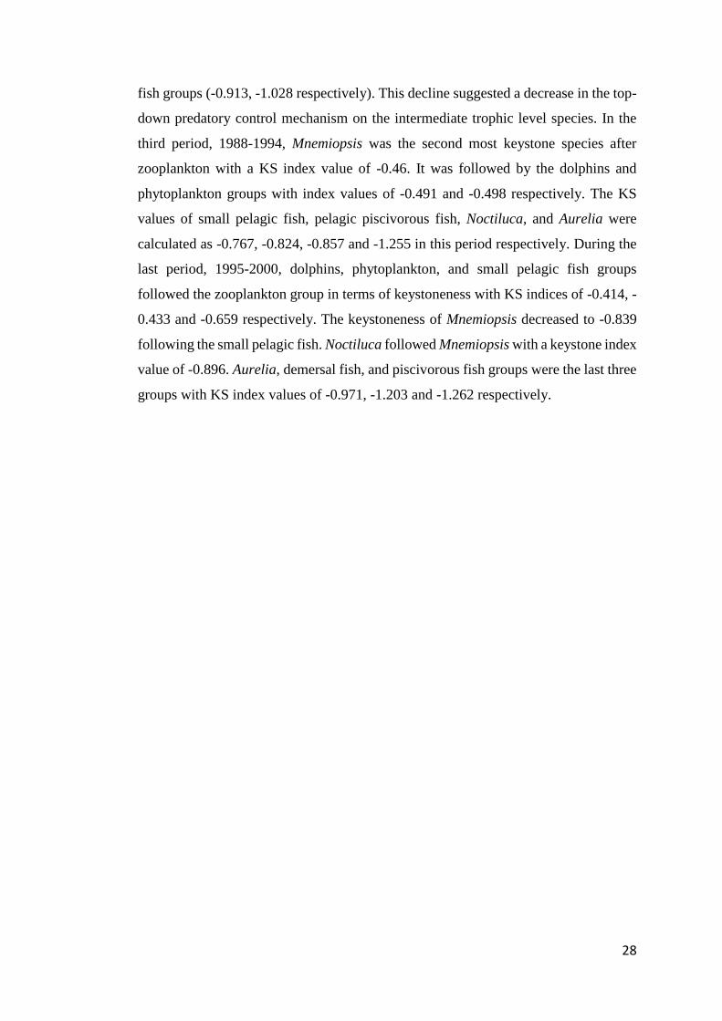
28
fish groups (-0.913, -1.028 respectively). This decline suggested a decrease in the top-
down predatory control mechanism on the intermediate trophic level species. In the
third period, 1988-1994, Mnemiopsis was the second most keystone species after
zooplankton with a KS index value of -0.46. It was followed by the dolphins and
phytoplankton groups with index values of -0.491 and -0.498 respectively. The KS
values of small pelagic fish, pelagic piscivorous fish, Noctiluca, and Aurelia were
calculated as -0.767, -0.824, -0.857 and -1.255 in this period respectively. During the
last period, 1995-2000, dolphins, phytoplankton, and small pelagic fish groups
followed the zooplankton group in terms of keystoneness with KS indices of -0.414, -
0.433 and -0.659 respectively. The keystoneness of Mnemiopsis decreased to -0.839
following the small pelagic fish. Noctiluca followed Mnemiopsis with a keystone index
value of -0.896. Aurelia, demersal fish, and piscivorous fish groups were the last three
groups with KS index values of -0.971, -1.203 and -1.262 respectively.
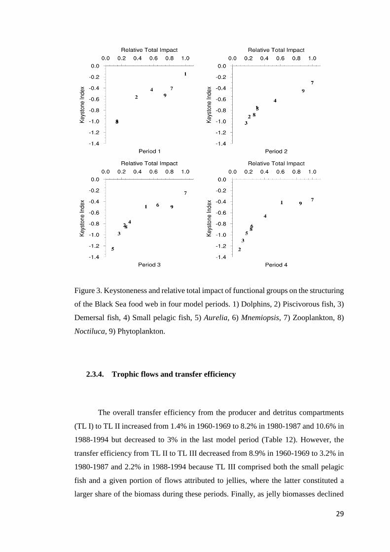
29
Figure 3. Keystoneness and relative total impact of functional groups on the structuring
of the Black Sea food web in four model periods. 1) Dolphins, 2) Piscivorous fish, 3)
Demersal fish, 4) Small pelagic fish, 5) Aurelia, 6) Mnemiopsis, 7) Zooplankton, 8)
Noctiluca, 9) Phytoplankton.
2.3.4. Trophic flows and transfer efficiency
The overall transfer efficiency from the producer and detritus compartments
(TL I) to TL II increased from 1.4% in 1960-1969 to 8.2% in 1980-1987 and 10.6% in
1988-1994 but decreased to 3% in the last model period (Table 12). However, the
transfer efficiency from TL II to TL III decreased from 8.9% in 1960-1969 to 3.2% in
1980-1987 and 2.2% in 1988-1994 because TL III comprised both the small pelagic
fish and a given portion of flows attributed to jellies, where the latter constituted a
larger share of the biomass during these periods. Finally, as jelly biomasses declined
30
to moderate values, the transfer efficiency from TL II to TL III increased slightly to
3.8% in period 1995-2000. The transfer efficiencies of all flows from TL III to TL IV
were calculated as 6.3%, 7.3%, 8.7% and 7.4% in the four modelled periods,
respectively. Considering the transfer efficiencies from TL IV to TL V, a rough
estimate of 0.5% was calculated for each period; however this estimate was biased by
the relatively low dolphin biomass due to the lack of reliable observational data.
Table 12. Transfer efficiency of flows across trophic levels in the four modelled
periods.
Source \
Trophic
level
1960-1969 1980-1987 1989-1994 1995-2000
II III IV V II III IV V II III IV V II III IV V
Producer 1.4 9.0 6.3 0.5 8.2 3.2 7.3 0.5 10.8 2.2 8.7 0.5 3.0 3.8 7.4 0.5
Detritus 1.4 8.9 6.3 0.5 8.3 3.2 7.3 0.5 10.3 2.2 8.7 0.5 3.0 3.8 7.4 0.5
All flows 1.4 8.9 6.3 0.5 8.2 3.2 7.3 0.5 10.6 2.2 8.7 0.5 3.0 3.8 7.4 0.5
2.3.5. Summary statistics and synthetic indicators
The results of the analyses of the synthetic indicators and the statistical
parameters (

31
Table 13) calculated for the four model periods were summarised in this
section. Total System Throughput (TST) increased from 681.733 gC m-2 y-1 in the
period 1960-1969 up to 1,405.977 gC m-2 y-1 in 1980-1987 with increasing productive
capacity of the ecosystem due to eutrophication. In the periods 1988-1994 and 1995-
2000, TST values were calculated as 1,316.583 gC m-2 y-1 and 1,020.347 gC m-2 y-1
respectively.

32
Table 13. Summary statistics of the four mass-balance models of the Black Sea
ecosystem for their respective periods.
Parameter/Period 1960-1969 1980-1987 1988-1994 1995-2000 Units
Summary Statistics
Sum of all consumption 234 381 247 450 gC m-2 y-1
Sum of all exports 99 318 411 49 gC m-2 y-1
Sum of all respiratory
flows 157 250 157 299 gC m-2 y-1
Sum of all flows into
detritus 191 458 502 223 gC m-2 y-1
Total system throughput 682 1,406 1,317 1,021 gC m-2 y-1
Sum of all production 286 623 608 408 gC m-2 y-1
Mean trophic level of the
catch 3.36 3.07 3.1 3.0 -
Gross efficiency
(catch/net p.p.) 0.000 0.001 0.000 0.001 -
Calculated total net
primary production 256 567 567 347 gC m-2 y-1
Total primary
production / total
respiration 1.63 2.27 3.61 1.16 -
Net system production 99 318 410 49 gC m-2 y-1
Total primary
production / total
biomass 1320 91 117 90 year-1
Total biomass / total
throughput 0.003 0.004 0.004 0.004 year-1
Total biomass (excluding
detritus) 1.94 6.24 4.86 3.87 gC m-2
Primary Production
Required / Total PP
(PPR/TotPP) 6.87 52.82 25.84 28.93 %
Network Flow Indices
System Omnivory Index 0.072 0.122 0.115 0.116 -
Finn’s Cycling Index 9.40 4.61 2.76 15.01 (% of
TST)
Finn’s mean path length 2.662 2.477 2.320 2.936 -
Net system production increased from 98.934 gC m-2 y-1 in 1960-1969 to
317.918 gC m-2 y-1 in period 1980-1987. In the periods 1988-1994 and 1995-2000, net
system production was calculated as 410.443 gC m-2 y-1 and 48.563 gC m-2 y-1
respectively. The ratio of total primary production to the sum of all respiratory flows

33
in the system was calculated as 1.63 in 1960-1969. In period 1980-1987, this ratio
increased to 2.274. It further increased to 3.614 in 1988-1995. In the last period of
1995-2000, this ratio decreased to 1.162.
The mean trophic level of catches (mTLc) decreased from 3.36 in 1960-1969
to 3.07 in period 1980-1987. mTLc values were calculated as 3.10 and 3.03 in the
periods 1988-1994 and 1995-2000 respectively. Furthermore, the catches by trophic
levels showed that different trophic levels dominated the fisheries catches in particular
periods (Table 14). In period 1960-1969, TL III and TL IV constituted 64% and 35%
of the entire fisheries yield in the system respectively. In 1980-1987, the percentage of
TL IV organisms in fisheries catches decreased to 7.8% whereas TL III species
constituted 90% of the yield. In 1988-1995, the catch composition comprised 82% of
TL III groups and 12.6% of TL IV groups. In the last period 1995-2000, the percentage
of TL IV organisms in the catches decreased to 4.5% whereas TL III organisms
increased to 92%. Similarly, the biomass distribution by trophic levels in the system
reflected the dominance of different trophic level species in the four model periods
(Table 15). The ecosystem was dominated by TL IV and TL III organisms which
represented 64.5% and 35% of all biomasses respectively in period 1960-1969
illustrating the dominance of higher-trophic-level groups within the ecosystem. In
period 1980-1987, TL III organisms constituted over 90% of the total biomass within
the ecosystem whereas TL IV organisms decreased to 7.7%. This was the result of the
removal of top predatory species from the ecosystem by fisheries. The percentage of
TL IV organisms in the total living biomass increased to 12.5% when TL III organisms
decreased to 83% in period 1988-1995. This was a direct consequence of the collapse
of small pelagic fish stocks, which in turn, reflected as an increase in the relative
biomass proportion of higher-trophic-level species in the community. In the last period
(1995-2000), the proportion of TL IV organisms decreased to 5% and TL III organisms
increased to 92% due to the recovery of the small pelagic fish stocks.

34
Table 14. Catches by trophic levels in four modelled periods of the Black Sea.
Trophic Level 1960-1969 1980-1987 1988-1994 1995-2000
V 0.00004 0.00004 0.00004 0.00004
IV 0.0109 0.0355 0.0266 0.0133
III 0.02 0.415 0.175 0.249
II 0 0.00824 0.00937 0.00614
I 0 0 0 0
Table 15. Living biomass by trophic levels in four modelled periods of the Black Sea.
Trophic Level 1960-1969 1980-1987 1988-1994 1995-2000
V 0.0004 0.0004 0.0004 0.0004
IV 0.0487 0.187 0.0878 0.0558
III 0.24 1.929 1.142 0.8
II 0.771 2.172 1.679 1.817
I 0.88 1.95 1.95 1.194
Finn’s Cycling Index (FCI) decreased from 9.4% in 1960-1969 to 4.61% in
1980-1987. It further decreased down to 2.76% in 1988-1994. This indicated that
energy turnover in the food web decreased from 1960-1969 to periods 1980-1987 and
1988-1994. The FCI increased to 15.01% in period 1995-2000 due to a slight
ecosystem-wide recovery, i.e. improving transfer efficiency rates of trophic flows
through the food web and reduction in the proportion of the short-circuited energy
flows, in response to the reduced eutrophication and the introduction of Mnemiopsis-
predator Beroe. This impact was also reflected in the Finn’s mean path length which
was calculated as 2.662, 2.477, 2.320 in periods 1960-1969, 1980-1987, and 1988-
1994 respectively, showing a shortening in the average distance of a unit of energy
travelled within the food web as the system degraded (i.e. short-circuiting of energy
flows) in periods 1980-1987 and 1988-1994. A subsequent increase in Finn’s mean
path length to 2.936 in 1995-2000 agreed with the slight recovery observed in
ecosystem conditions.
The biomass ratios of Aurelia, Mnemiopsis and Noctiluca, which could be
considered as r-strategist species, to the community biomass in general and plankton
biomass in particular, increased from 0.0435 in 1960-1969 to 0.347 and 0.633 in
35
periods 1980-1987 and 1988-1994 respectively. This reflected the increased
perturbations, i.e. stress conditions sensu Odum (1985), which prevailed in the Black
Sea ecosystem during these latter periods.
2.4. Discussions and conclusions
2.4.1. Considerations specific to the methodology
The chapter of the thesis considerably utilised parameterisations of previous
mass-balance modelling studies in the Black Sea with minor modifications and
followed a similar modelling scheme, however, it elaborated these former
contributions by focusing on the ecosystem functioning itself through energetic flows
and prey-predator interactions with the help of synthetically produced trophic
indicators. Further, it included important functional groups such as dolphins and
Mnemiopsis, which were not considered in the previous studies utilising Ecopath
models. These aspects of this chapter differed from the similar earlier studies and up
till now this had been a deficiency in the literature shadowing the understanding of the
trophic characteristics of the changes the Black Sea ecosystem had undergone in the
second half of the 20th century.
The simplicity of the model scheme, i.e. the inclusion of a limited number of
functional groups, was designed purposefully in order not to overcomplicate the
models to cause increasing source of uncertainty in the model outputs due to the
increased number of parameters required to set up the models. However, the modelling
scheme was capable of adequately representing the general structure of the Black Sea
food web so as to derive interpretations from ecological indicators calculated utilising
the food web’s functional properties. It was more of a concern for this chapter to
examine the characteristics of the food web over the model periods by focusing on
traits of organisms rather than dealing with specific species dynamics within the
ecosystem.
In this chapter of the thesis, it was assumed that the EE values calculated by

36
the mass-balance model set-up in the first period of the Black Sea for dolphins and
pelagic piscivorous fish groups would approximately remain unchanged in the latter
model periods. This assumption might have significantly impacted the calculated
values of indicators such as keystoneness for these groups. Therefore, this situation
should be noted when evaluating the results of the keystoneness analysis. However,
considering the complete absence of stock assessment studies for these two functional
groups, this assumption was inevitable. Further, the exploitation levels of pelagic
piscivorous fish should have remained approximately stable over the years if the high
fisheries demand on these fishes was acknowledged (Gucu, 2002; Oguz, 2007; Oguz
et al., 2008b), hence leading to high EE estimates used in the mass-balance models.
Pelagic piscivorous fish in the Black Sea have always been under exceeding levels of
exploitation and their predators have been limited in the system. Hence, it could be
assumed that EE values for this functional group might have fluctuated around the
same mean value over the four modelled periods. On the other hand, dolphins had been
exploited intensively in the Black Sea until the ban of its fisheries in 1966 in USSR,
Bulgaria and Romania and finally in 1983 in Turkey. Therefore, a decreasing EE value
was most likely to be expected for dolphins group over the four modelled periods. In
this aspect, it could be stated that mass-balance model set-ups in this chapter led to
relatively higher estimates of natural mortality values for this group. However, by-
catch has been a significant mortality source for dolphins even after the dolphin
fisheries ban in the Black Sea (2000-3000 individuals per year, Ozturk et al., 1999),
which might have compensated the release of fishing pressure on this group after the
fishing bans so as to cause high “natural” mortality levels.
2.4.2. Interpretation of model results
This chapter of the thesis provided an assessment of the Black Sea ecosystem
structure and functioning using the ecological indicator approach pioneered by Odum
(1969, 1985) and elaborated upon by many others (Ulanowicz and Puccia, 1990;
Christensen, 1995; Costanza and Mageau, 1999; Ulanowicz, 2004; Shannon et al.,
2009; Gaichas et al., 2009). A similar approach was previously implemented in the
Black Sea by Christensen and Caddy (1993) with limited scope that compared the pre-

37
Mnemiopsis (early 1980s) and post-Mnemiopsis (early 1990s) eras and examined the
likely impacts of introduction of Beroe ovata on the Mnemiopsis population. This
chapter’s work expanded upon this in terms of complexity of analysis and time periods
of the ecosystem examined. It differed from those of Gucu (2002) and Daskalov (2002)
because of the interpretation of model products since the mass-balance modelling in
this chapter comprised the entire food web and its quantitative analysis through the use
of ecological indicators to assess the ecosystem status prevailed in the Black Sea
during the last few decades.
Evidence of top-down control in the first period (1960-69) was demonstrated
by the highest KS value belonging to dolphins group in the food web. One interesting
outcome of the analysis was the lack of recovery of dolphins even though the dolphin
fishery was banned after 1966 in USSR, Bulgaria, Romania and 1983 in Turkey
(Birkun, 2008). This was clearly supported by the MTI and transfer efficiency (TE)
analyses. In MTI analysis, the continuous increase in the negative impact of fisheries
on dolphins even after the fishing ban suggested that excessive harvesting of small
pelagic fish did not leave sufficient food resources for dolphins to promote their
population growth, hence, consolidated the indirect negative impact of fisheries on
dolphins. TE analysis further quantified increasing resource supply to TL II in
accordance with intensive eutrophication, but this did not propagate further up in the
food web due to the short-circuiting of energy flows by the gelatinous population
which dominated the food web. This short-circuiting and the decrease in energy
transfer efficiency to higher trophic levels were also signified by the decrease in Finn’s
Cycling and Finn’s Mean Path Length indicators starting from the first period. Further
basis for the severity of this short-circuiting effect was provided by the KS value of
Mnemiopsis in 1988-1994, which suggested Mnemiopsis as being the second most
significant keystone species after the zooplankton group.
The impact of intensive eutrophication was also reflected in the TST values of
the ecosystem which increased almost two-fold between the first and second model
periods. This reversal in the food web from a top-down controlled state to become
more influenced by bottom-up controls was demonstrated by the highest keystone
values calculated for zooplankton and phytoplankton groups in the latter three model
periods. Fisheries also played an important role in this reorganisation as depicted by
the decrease in the mean trophic level of catch (mTLc) and the mean trophic level of

38
community (mTLco) indices due to selective extraction of particular fish groups from
the ecosystem so that top-down control on the food web abated. This “fishing down
the food web” (Pauly et al., 1998) impact has been continuing in the Black Sea since
the 1960s.
In accordance with the notion defined by Odum (1985), the stability of the
Black Sea ecosystem had been regressed from many aspects. The net system
production, an indicator expected to be close to zero in mature ecosystems, increased
roughly three-fold from the first period to the latter two periods. Similarly, the TPP/TR
ratio increased by about four-fold from a close-to-unity value (typical for healthy
ecosystems) in the first time period to the subsequent time periods also suggesting this
deterioration (growing instability) in the ecosystem. The biomass ratio of the sum of
opportunistic species Mnemiopsis, Aurelia, and Noctiluca with respect to the total
zooplankton increased by more than an order of magnitude from the first period to
period 1988-1994. These species had no natural predators within the Black Sea
ecosystem. Hence, the accumulated energy in their respective TLs of these organisms
was not transferred upwards in the trophic chain but was circuited back to detritus by
means of natural mortality. This leakage in the food web reduced the TE of flows
through the trophic chain up to TL III (Figure 4).
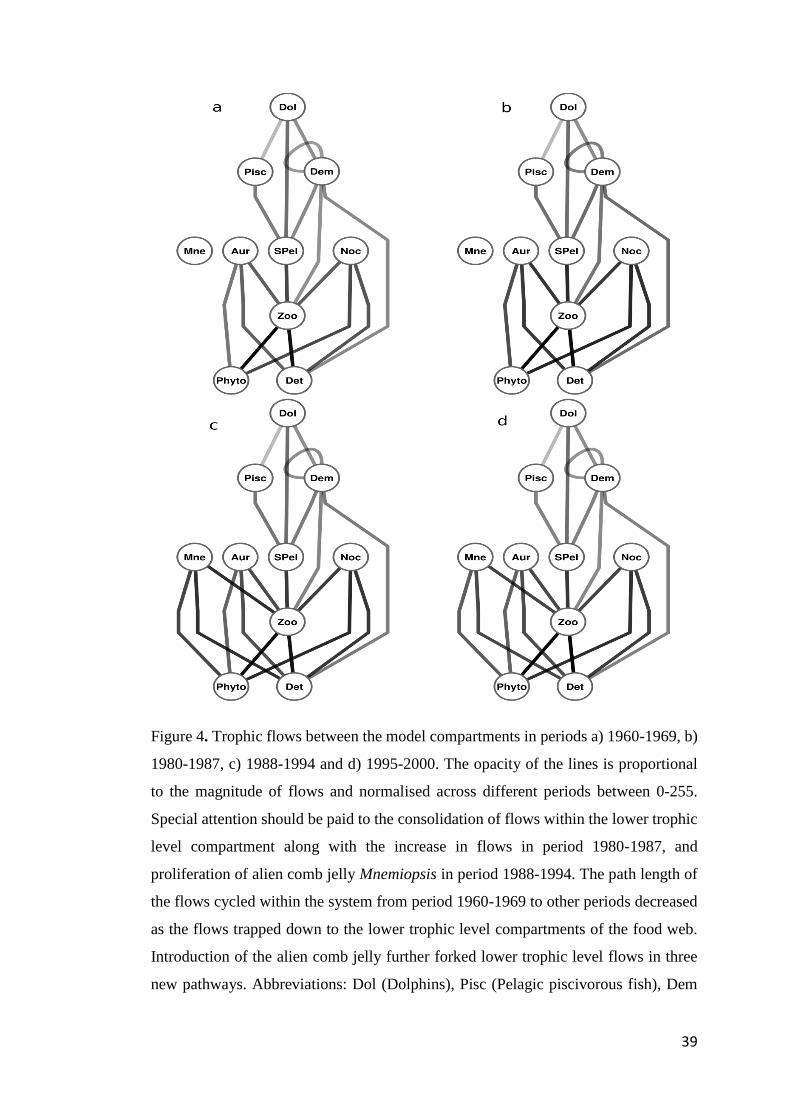
39
Figure 4. Trophic flows between the model compartments in periods a) 1960-1969, b)
1980-1987, c) 1988-1994 and d) 1995-2000. The opacity of the lines is proportional
to the magnitude of flows and normalised across different periods between 0-255.
Special attention should be paid to the consolidation of flows within the lower trophic
level compartment along with the increase in flows in period 1980-1987, and
proliferation of alien comb jelly Mnemiopsis in period 1988-1994. The path length of
the flows cycled within the system from period 1960-1969 to other periods decreased
as the flows trapped down to the lower trophic level compartments of the food web.
Introduction of the alien comb jelly further forked lower trophic level flows in three
new pathways. Abbreviations: Dol (Dolphins), Pisc (Pelagic piscivorous fish), Dem

40
(Demersal fish), SPel (Small pelagic fish), Aur (Aurelia), Mne (Mnemiopsis), Noc
(Noctiluca), Zoo (Zooplankton), Phyto (Phytoplankton), Det (Detritus).
In conclusion, contrary to Gucu (2002) and Daskalov (2002) who suggested
overfishing as the prime cause of the collapse of small pelagic fish stocks in 1989,
according to the analyses in this chapter I conclude that this collapse was most
probably related to more than one single cause. Indeed, overexploitation by fisheries
was severe and evident in the various system indices, such as i) the decrease in the
mean trophic level catches from 3.34 in 1960-1969 down to 3.07 in 1980-1987, ii) the
increase in primary production required to support catches from 6.87 % in 1960-1969
to 52.82 % in period 1980-1987, and iii) the increase in proportion of opportunistic
species within the plankton community. Further, the impact of increased competition
between gelatinous organisms and small pelagic fish for resources as calculated in the
MTI analysis with increasing negative impact index values between these groups in
period three and four provided an additional strong explanation for the collapse. The
negative impact of trophic competition between Aurelia and small pelagic fish in 1980-
1987 was demonstrated by the MTI analysis. This trophic competition was further
exacerbated by the proliferation of Mnemiopsis as shown by the strong negative impact
between Mnemiopsis and small pelagic fish in period 1988-1994. Based on what was
demonstrated by the ecological indicators and statistical properties of the Black Sea
ecosystem examined in this chapter, I propose that the synergistic effects of “resource
competition” with jellyfish and “overexploitation” by fisheries were the most likely
causes to lead such a collapse in the small pelagic fish stocks in 1989.
Using the Black Sea ecosystem as a case study, this chapter of the thesis
validated that the structure and functioning of a marine ecosystem can be examined
coherently through a carefully selected set of ecological indicators even by utilising a
simple mass-balance model such as Ecopath. Moreover, if complemented by a time-
dynamic Ecosim model of the Black Sea of similar or a more detailed food web
complexity (chapters 3 and 5), and further supplemented by the application of network
analyses to obtain dynamically varying ecological indicators used in this chapter, the
findings of this section may be regarded as a simplistic but quantitative assessment of
the Black Sea’s food web structure and functioning over the last few decades in order
to provide a baseline towards establishing the goal of "integrated ecosystem
assessment" (Levin et al. 2009) for the region.

41
3. CHAPTER: Modelling regime shifts of the Black Sea food web
dynamics using a complex food web representation
3.1. Introduction
For more than a decade, regime shifts; i.e. persistent changes in the
ecosystems’ organisation, structure and functioning (Kinzig et al., 2006), have been a
special focus in marine research in link with the impacts of anthropogenic forcing on
climate and ecosystems (Steele, 1998, 2004). Recent studies have been increasingly
focused on regime-shift phenomena along with the recent advances in ecological and
statistical modelling tools that enabled both diagnostic and prognostic analyses under
different environmental scenarios and anthropogenic impacts (e.g. Reid et al., 2001;
Beaugrand, 2004; Daskalov et al., 2003, 2007; Möllmann et al., 2008, 2009; Llope et
al., 2011). Ecosystem models have recently emerged as important tools to develop
Ecosystem-Based Management (EBM) strategies to address community-scale
ecological questions (e.g. Fulton et al., 2005; Plaganyi, 2007) under changing regimes
as well as investigating historical progressions of ecosystems. Lower trophic level
models have long been used in this respect for the investigation of the consequences
of intrinsic and extrinsic pressures on marine ecosystems (e.g. Oguz et al., 2001;
Salihoglu, 2009; Salihoglu et al., 2011). During recent decades, together with the
advancement of higher trophic level models focusing on fish, end-to-end ecosystem
models, which represent the ecosystem from biogeochemical processes up to top
predators, that would provide a holistic understanding of the changes in marine
ecosystems with respect to climatic and anthropogenic impacts started to develop
(Fulton, 2010).
Ecopath with Ecosim has emerged as one of the most widely acclaimed higher
trophic level model and has been applied to a great range of marine and freshwater
ecosystems for more than two decades. Specifically in the last decade, with the
recognition of the usefulness of such end-to-end holistic modelling approaches,
Ecopath and Ecosim models have been used to investigate regime shifts and/or system
reorganisations in marine ecosystems, with or without coupling with lower trophic

42
level and hydrodynamic models, using indicator-based assessment methods which
inspected the ecosystem in question through a set of ecological indicators (Fulton et
al., 2005; Coll et al., 2006, 2009). This indicator-based ecosystem assessment was
pioneered by Odum (1969), who formed the basis of the approach known today as “the
ecosystem theory”. In his pioneering work entitled “The Strategy of Ecosystem
Development”, Odum quantified many aspects of ecosystem development through
various statistical parameters and indicators of ecosystems and put forward their
expected behaviours under changing ecological conditions so as to determine its
properties of structure, i.e. the organisation of organisms across the food web, and
functioning, i.e. properties of energetic flows transferred through various trophic levels
from grazing and detritus-based food chains. Only after quantifying these attributes
and properties, it could have been possible to deduce whether a given ecosystem was
under stress, e.g. exposed to anthropogenic pressure like overfishing, or balancing
itself and its processes (ecological homeostasis, Odum (1985)). This pioneering work
was further elaborated by many ecologists over the course of time (Odum, 1985;
Shaeffer et al., 1988; Christensen, 1995; Rapport et al., 1992, 1998; Costanza and
Mageau, 1999; Shannon et al., 2009; Shin et al., 2010b, c) and applied to a number of
ecosystems, either marine or terrestrial, across the world (Christensen and Cury, 2005;
Cury and Christensen, 2005; Shin et al., 2005). Furthermore, it was developed to
include indicators and parameters derived synthetically from “ecological network
theory” (Ulanowicz, 1986). Such studies on fishery and ecosystem related indicators
have been presented by Coll et al. (2005, 2006) and Fulton et al. (2005) showing
usefulness of such trophodynamic indicators in ecosystems analysis. Similar tools to
investigate changes in the food web structure under different pressures were recently
used by Cury et al. (2005), Guénette et al. (2006) and Travers et al. (2010). Further,
Fulton et al. (2005) demonstrated the effectiveness of ecological indicators as the most
reliable tools to investigate the ecosystem impacts of fishing by providing the
characterisation of ecosystem state and indicating the causality of the changes it had
undergone. All these studies proved the effectiveness of using ecological indicators in
assessing ecosystem changes over a long period of time and investigating their
likely/unlikely consequences. In this aspect, this chapter of this thesis work was
dedicated to investigating the presence of different regimes in the food web
dynamics and ecosystem properties of the Black Sea in a holistic approach using
synthetically obtained time series of ecosystem indicators so as to support the

43
findings of indicator-based mass-balance model analysis in the previous chapter.
This chapter further investigated the presence of significant changes in the Black
Sea ecosystem in the second half of the 20th century that could be attributed as
different persistent regimes.
3.2. Materials and Methods
The mass-balance Ecopath model of the Black Sea detailed in section 2.2.1 was
further developed by disaggregating the functional groups of small pelagic fish,
pelagic piscivorous fish and demersal fish, which were aggregated guilds of multiple
species, into individual species components. Further, new state variables were
introduced; i.e. two new jellyfish species and another detritus compartment; particulate
organic matter (POM). The model was extended to include twenty-two functional
groups, which comprised twelve fish groups; Black Sea anchovy (Engraulis
encrasicolus ponticus; Alexandrov, 1927), Black Sea sprat (Sprattus sprattus
phalaericus; Risso, 1827), Black Sea horse mackerel (Trachurus mediterraneaus
ponticus; Aleev, 1956), Atlantic bonito (Sarda sarda; Bloch, 1973), bluefish
(Pomatomus saltator; Linnaeus, 1776), Atlantic mackerel (Scomber scombrus;
Linnaeus, 1758), turbot (Psetta maeotica, Pallas, 1814), Black Sea whiting
(Merlangius merlangus euxinus, Nordmann, 1840), spiny dogfish (Squalus acanthias,
Linnaeus, 1758) and Black Sea striped mullet (Mullus barbatus ponticus, Essipov,
1927), four jellyfish; Mnemiopsis leidyi (Agassiz, 1865), Aurelia aurita (Linnaeus,
1758), Pleurobrachia spp. and Beroe ovata (Mayer, 1912); two detritus groups; one
sediment and one representing particulate organic matter (POM); one phytoplankton
and one zooplankton group due to lack of time series data for functional sub-groups;
one heterotrophic dinoflagellate Noctiluca scintillans (Ehrenberg, 1834) and one
dolphins group to represent the Black Sea marine mammals, which were mainly
composed of Black Sea common dolphin (Delphinus delphis spp. ponticus; Barabash-
Nikiforov, 1935), Black Sea bottlenose dolphin (Tursiops truncatus spp. ponticus;
Barabasch, 1940) and Black Sea harbour porpoise (Phocoena phocoena spp. relicta;
Abel, 1905) (Table 16, Figure 5). Anchovy was defined as a multi-compartment group
and was represented with two subgroups; one for `eggs and larvae`, and the other for

44
`adult` life stages. The compartments were linked to each other by means of von
Bertalanffy growth function (VBGF). Three fishing types were identified; trawlers,
purse seiners and gill-netters to represent the fishery impact on the ecosystem.
Figure 5. Schematic view of the Black Sea time-dynamic Ecopath with Ecosim model.
Horizontal straight lines which are numbered with integers on the y-axis denote trophic
levels. Arches show flows between groups. Nodes are the state variables and
proportional to the biomass of groups in 1960.
The model currency was chosen as gC m-2 y-1 based on the reasons detailed in
section 2.2.1. The in-situ biomass data and catch statistics, which were used to fit the
model, were available in wet weight and converted to the model currency using the
specified wet-weight to grams carbon conversion multipliers given in Table 7.
The mass-balance model was setup and balanced for the quasi-pristine
conditions of the early 1960s based on the mass-balance model of the first period in
Chapter 2. For this purpose, the P/B and Q/B values of aggregated groups in the
simplified mass-balance models of Chapter 2 were used for the individual species
forming the corresponding group in this chapter’s model, which included
representations at the individual species level. For instance, the P/B and Q/B values of

45
small pelagic fish group in the Ecopath model of the first period in chapter 2 were used
for the species which formed the small pelagic fish group; i.e. horse mackerel, shad,
sprat, and anchovy in this chapter’s model. Similarly, the pelagic piscivorous fish;
Atlantic bonito, bluefish and Atlantic mackerel, and demersal fish; turbot, whiting, red
mullet and spiny dogfish, were parameterised using the same approach. The input
biomass and catch values of the fish species were obtained from Prodanov et al.,
(1997). For the fish species with no biomass estimates for the initial year, an EE value
of 0.9 was assumed.
Concerning groups/species other than fish and dolphins, data from Shiganova
(2008) were used for input biomass values except for the phytoplankton group. For
phytoplankton, input biomass value was taken from Nesterova (2008). Although
Mnemiopsis and Beroe species were not present in the ecosystem conditions of 1960s
and introduced in late 1980s and 1990s respectively, these two species were included
in the model set-up of 1960s because it was not possible to introduce these two groups
into the ecosystem at their specific year of introduction unless included in the initial
model set-up. Therefore, their input biomass values were set to unrealistically low
values in order to prevent them interacting within the food web with other components
of the model until their year of introduction.
All of the basic input parameters (Table 16) were then perturbed within 20 %
coefficient of variation using a Monte-Carlo style parameter search routine in EwE in
order to obtain the best fitting combination of initial conditions to the time series used
to fit the model.
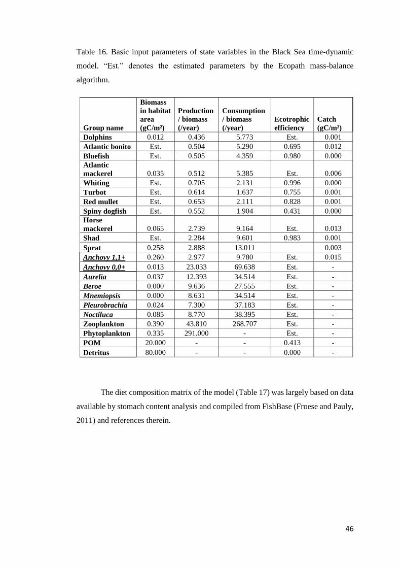
46
Table 16. Basic input parameters of state variables in the Black Sea time-dynamic
model. “Est.” denotes the estimated parameters by the Ecopath mass-balance
algorithm.
Group name
Biomass
in habitat
area
(gC/m²)
Production
/ biomass
(/year)
Consumption
/ biomass
(/year)
Ecotrophic
efficiency
Catch
(gC/m²)
Dolphins 0.012 0.436 5.773 Est. 0.001
Atlantic bonito Est. 0.504 5.290 0.695 0.012
Bluefish Est. 0.505 4.359 0.980 0.000
Atlantic
mackerel 0.035 0.512 5.385 Est. 0.006
Whiting Est. 0.705 2.131 0.996 0.000
Turbot Est. 0.614 1.637 0.755 0.001
Red mullet Est. 0.653 2.111 0.828 0.001
Spiny dogfish Est. 0.552 1.904 0.431 0.000
Horse
mackerel 0.065 2.739 9.164 Est. 0.013
Shad Est. 2.284 9.601 0.983 0.001
Sprat 0.258 2.888 13.011 0.003
Anchovy 1,1+ 0.260 2.977 9.780 Est. 0.015
Anchovy 0,0+ 0.013 23.033 69.638 Est. -
Aurelia 0.037 12.393 34.514 Est. -
Beroe 0.000 9.636 27.555 Est. -
Mnemiopsis 0.000 8.631 34.514 Est. -
Pleurobrachia 0.024 7.300 37.183 Est. -
Noctiluca 0.085 8.770 38.395 Est. -
Zooplankton 0.390 43.810 268.707 Est. -
Phytoplankton 0.335 291.000 - Est. -
POM 20.000 - - 0.413 -
Detritus 80.000 - - 0.000 -
The diet composition matrix of the model (Table 17) was largely based on data
available by stomach content analysis and compiled from FishBase (Froese and Pauly,
2011) and references therein.
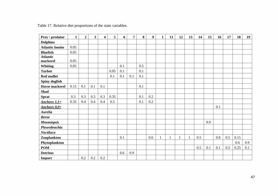
47
Table 17. Relative diet proportions of the state variables.
Prey \ predator 1 2 3 4 5 6 7 8 9 1 11 12 13 14 15 16 17 18 19
Dolphins
Atlantic bonito 0.05
Bluefish 0.05
Atlantic
mackerel 0.05
Whiting 0.05 0.1 0.5
Turbot 0.05 0.1 0.1
Red mullet 0.1 0.1 0.1 0.1
Spiny dogfish
Horse mackerel 0.15 0.1 0.1 0.1 0.1
Shad
Sprat 0.3 0.3 0.3 0.3 0.35 0.1 0.2
Anchovy 1,1+ 0.35 0.4 0.4 0.4 0.5 0.1 0.2
Anchovy 0,0+ 0.1
Aurelia
Beroe
Mnemiopsis 0.9
Pleurobrachia
Noctiluca
Zooplankton 0.1 0.6 1 1 1 1 0.5 0.8 0.5 0.15
Phytoplankton 0.6 0.9
POM 0.5 0.1 0.1 0.5 0.25 0.1
Detritus 0.6 0.9
Import 0.2 0.2 0.2

48
Concerning lower trophic level groups, the biomass estimations from in-situ
sampling data were used to fit their simulated biomass values. For the zooplankton
group, the data were obtained from Shiganova (2008) and for the phytoplankton group
the data obtained from Nesterova (2008) were used. However, the zooplankton groups
that had no natural predators in the ecosystem, i.e. Aurelia, Pleurobrachia, Noctiluca,
Mnemiopsis (until 1997) and Beroe, were forced with biomass estimates obtained from
in-situ samplings. The primary productivity of the phytoplankton group was forced
using calculations from Oguz et al. (2012).
The dynamic model of the Black Sea was run starting from the year 1960 until
the end of the year 1999. The fish groups were forced with time series of fishing
mortality estimates obtained from conventional models (e.g. Virtual Population
Analysis (VPA)). The time series of catch data and VPA biomass estimations of fish
groups used to fit the model and the time series of fishing mortality values used to
force the fish groups were taken from Prodanov et al. (1997) for the years (1960-1992)
and complemented from Shlyakhov (2008) for the years 1993-1999. However, time
series of catch and VPA biomass estimations had occasional gaps and these were left
missing. Concerning fishing mortalities, the missing values at the start/end of the time
series were complemented by continuing the first/last fishing mortality value until the
beginning/end year of the simulation. For groups that completely lacked fishing
mortality estimates, hence, biomass estimations, the fishing mortality values were
estimated so as to achieve better fits for the simulated catches to the statistical catch
data. However, the fishing mortalities for these groups were not changed year-to-year
but kept constant throughout the simulation period.
In the dynamic module of Ecopath with Ecosim, the mass-balance system of
linear equations of Ecopath detailed in the previous chapter was transferred to the time-
dynamic domain in the form of a differential equation:
𝑑𝐵𝑖𝑑𝑡
= (𝑃
𝑄)𝑖
∗∑𝑄𝑗𝑖
𝑘
𝑖=1
−∑𝑄𝑖𝑗
𝑘
𝑗=1
+ 𝐼𝑖 − (𝑀𝑖 + 𝐹𝑖 + 𝑒𝑖) ∗ 𝐵𝑖 (5)
where 𝑑𝐵𝑖/𝑑𝑡 is the rate of change of biomass (B) of group i over time t, (P/Q) is the
gross efficiency, ∑ Qji is the sum of the consumptions of group i, ∑ Qij is the sum of

49
the predation on group i, I is the immigration (incoming migration), M is the non-
predation mortality, F is the fisheries mortality and e is the emigration rate (outgoing
migration) of group i (Walters et al., 1997). This system of differential equations was
numerically integrated over time under the influence of forcing functions and initial
condition settings for the state variables.
3.2.1. Model Assessment
First, model skill assessments were carried out by evaluating the degree of fit
of simulated biomass and catch values with the VPA estimates of fish biomass, catch
statistics of fish groups and in-situ measurements of unforced lower trophic level
groups. The model was calibrated by tuning vulnerability (half-saturation) settings of
the functional groups as well as Monte-Carlo style parameter searching for the mass-
balance Ecopath model. For biomass and catch estimates simulated by the EwE model,
the goodness of fit measure was the weighted sum of squared deviations (SS, Mood et
al., 1974) of log biomasses/catches from the log predicted biomasses and/or catches
and Akaike Information Criterion (AIC; Akaike, 1974). For LTL groups, i.e.
zooplankton and phytoplankton biomass, the same measure of goodness of fit was
calculated against the in-situ time-series data from which biomass predictions were
obtained.
Similar to section 2.2.2, Ecological Network Analysis (ENA, Ulanowicz, 1986,
2004) was applied to the outputs of the dynamic Ecosim model in order to derive
synthetic indicators and system metrics of the ecosystem. Fluctuations of synthetic
indicators and system metrics over the simulation time of the dynamic model were
analysed using the annual biomass, catch and flow estimates. Afterwards, a sequential
algorithm based on the Student’s t-test (Student, 1908) for the detection of regime
shifts (Sequential T-test Analysis for the detection of Regime Shifts (STARS) analysis,
Rodionov, 2004) was applied to the indicators. This analysis is based on sequential
data processing in which the number of samples is not fixed and come in sequence.
For each new sample appended to the end of the data series, a t-test is applied to
determine whether a regime shift was present (Rodionov, 2004). Due to the presence

50
of significant autocorrelation in the time series of the synthetic indicators, pre-
whitening (Rodionov, 2006) was applied to the synthetic time series before applying
regime shift detection algorithm.
The ENA indicators in addition to those used in the evaluation of mass-balance
models were summarised in Table 18. Such synthetic indicators were valuable to
assess the ecosystem status and responses in different conditions as detailed in Odum
(1969) and discussed as ecosystem and fishery indicators in Christensen et al. (1995)
and Shannon et al. (2009).
Table 18. Ecosystem indices and synthetic ecological indicators used to assess the
ecological status of the Black Sea ecosystem with the Ecosim model.
Indicator Explanation
Ratios
Piscivorous fish to other fish ratio Expected to decrease with increased
exploitation.
Ratio of predatory fish biomass to forage
fish biomass
This ratio is an indicator of the “fishing
down the food web” effect as a result of
harvesting top predatory fish species. It is
expected to decrease with fishing
(Shannon et al., 2009).
Ratio of demersal fish to pelagic fish This ratio is an indicator of the “fishing
down the food web” effect as a result of
harvesting top predatory fish species. It is
expected to decrease with fishing.
(Shannon et al., 2009).
Ecosystem metrics
Biomass Total biomass of living groups in the
ecosystem.
Catch Total fisheries catches.
Kempton's Biodiversity Index (Q) Increase in this index indicates an increase
in biomass of high trophic level (TL >= III)
organisms (Kempton and Taylor, 1976). A
decrease would indicate a degraded state
(Shannon et al., 2009).
Fishing in balance index (FiB) FiB = 0 when a decrease/increase in TL is
matched by a corresponding respective
increase/decrease in catch. Increasing FiB
may indicate the geographic expansion of
the fishery or that it is now covering
previously underexploited stocks.
Decreasing FiB may indicate a collapsed
ecosystem or geographic contraction of the
fisheries (Shannon et al., 2009).

51
3.3. Results
3.3.1. Evaluation of Hindcast Model Results
The sum of squared deviations (SS) for 38 time series and AIC score for 76
data points were calculated as 470 and 576 respectively. Considering the gaps in time
series for most demersal species; i.e. whiting, turbot and spiny dogfish, and certain fish
species; bonito, bluefish and red mullet, did not have stock estimates but only catch
statistics, the SS and AIC values indicated that the model had a good fit and medium
uncertainty (Figure 6 and Figure 7).
Figure 6. Simulated biomass changes (solid lines) of the model compartments and their
degree of agreement with Virtual Population Analysis (VPA) estimates (dots) for fish
compartments and in-situ data (dots) for zooplankton and phytoplankton in the Black
Sea. The y-axis shows biomass in gC m-2 and the x-axis shows simulation years.
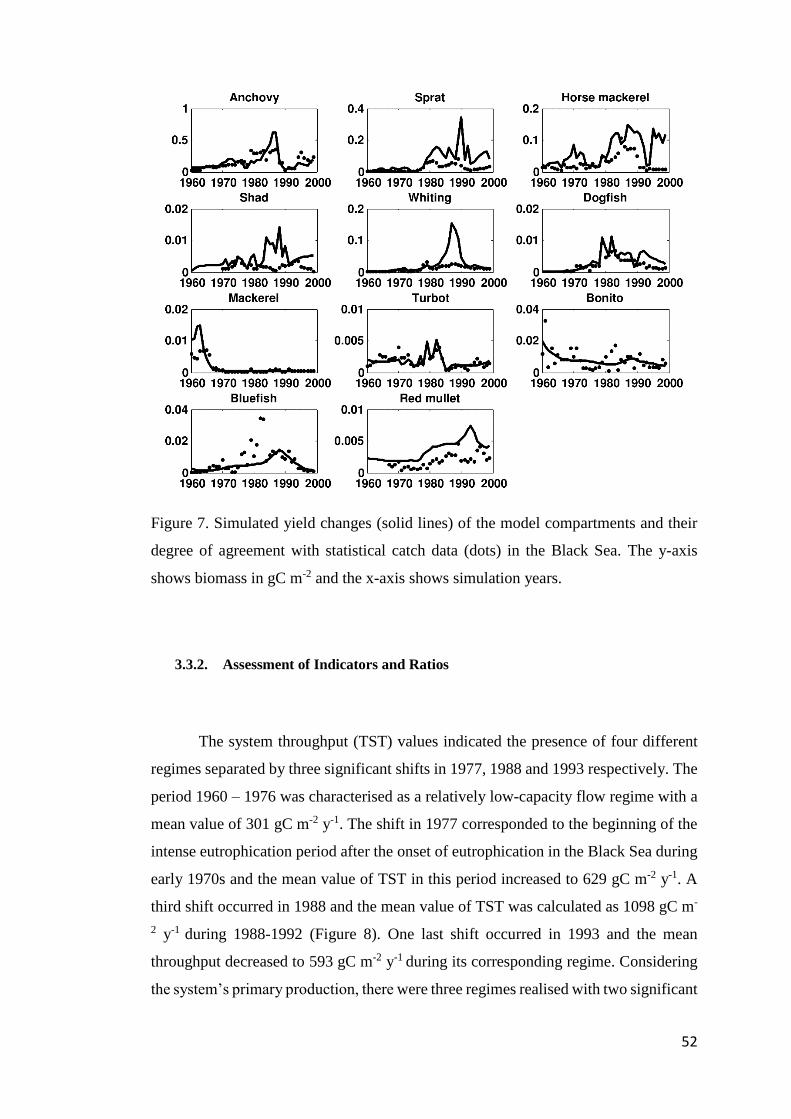
52
Figure 7. Simulated yield changes (solid lines) of the model compartments and their
degree of agreement with statistical catch data (dots) in the Black Sea. The y-axis
shows biomass in gC m-2 and the x-axis shows simulation years.
3.3.2. Assessment of Indicators and Ratios
The system throughput (TST) values indicated the presence of four different
regimes separated by three significant shifts in 1977, 1988 and 1993 respectively. The
period 1960 – 1976 was characterised as a relatively low-capacity flow regime with a
mean value of 301 gC m-2 y-1. The shift in 1977 corresponded to the beginning of the
intense eutrophication period after the onset of eutrophication in the Black Sea during
early 1970s and the mean value of TST in this period increased to 629 gC m-2 y-1. A
third shift occurred in 1988 and the mean value of TST was calculated as 1098 gC m-
2 y-1 during 1988-1992 (Figure 8). One last shift occurred in 1993 and the mean
throughput decreased to 593 gC m-2 y-1 during its corresponding regime. Considering
the system’s primary production, there were three regimes realised with two significant

53
shifts in 1978 and 1994. Further, the timing of these shifts almost matched the shifts
in TST occurred in 1977 and 1993 with a one year delay (Figure 8). The mean values
of primary production for these three regimes were calculated as125.7 mgC m-2 d-1,
494.0 mgC m-2 d-1 and 315.3 mgC m-2 d-1 respectively. These estimates were quite
close to the predictions given by Yunev et al. (2002) as; ~150 mgC m-2 d-1 before
1970s, ~600 mgC m-2 d-1 between 1980 and 1990, and ~300 mgC m-2 d-1 after 1990.
This showed that the fluctuations in the system’s primary production, which was a
consequence of changes in eutrophication, were the driving factor for the detected
regimes in the TST as well.
The STARS analysis of ascendency of the system indicated that two successive
regimes prevailed with mean values of 24.2% and 26.4% (Figure 8) separated with a
shift in 1976; which closely matched the onset of intense eutrophication. However,
considering the system overhead; i.e. resilience, four regimes were detected with shifts
in 1971, 1977 and 1994. The first three regimes were characterised by gradually
decreasing mean values of 45.2%, 42.5%, 36% respectively. During the last regime
began in 1994, the overhead value of the system increased slightly to 38.5% (Figure
8).
The recycling in the system (FCI) showed decreasing trends in the detected
first three regimes. The first regime change in the mean value of FCI occurred in 1968.
During 1960-1967, the mean value of FCI was calculated as 5.29. Afterwards until
1976, the mean FCI decreased to 3.89. In the third period starting with 1976, the mean
value of FCI further decreased and was calculated as 1.46. Finally, a last regime shift
occurred in 1994 and thereafter the mean value of FCI increased up to 2.32. This
showed that along with the increase in the system’s flow capacity, the cycling of
energy decreased significantly until 1994. This was in accordance with the increasing
populations of trophic dead-end species such as jellyfish and Noctiluca (Figure 8), all
of which diverted significant proportions of recycled matter back to detritus during
those corresponding years. With the decrease in the energetic capacity of the system
with alleviating eutrophic conditions starting with the collapse of the USSR in 1991
(Shiganova et al., 2008), the recycling of energy in the system increased (Figure 8) via
the limitation exerted on these opportunistic groups by constrained system production.
A similar pattern which supported this situation was detected by the STARS analysis
in the mean path length indicator (Figure 8) with detected regime shifts in 1968, 1977,

54
1988 and 1996. During the first four regimes, the mean path length travelled by a unit
of energy continuously decreased from a mean value of 2.60 in the first regime down
to mean values of 2.50, 2.37 and 2.32 in the latter three. In the last regime starting from
1996, the mean value of the mean path length indicator increased up to 2.37. These
two indicators suggested that along with the development of the ecosystem by means
of energetic capacity, the recycled energy in the system through the food web was
confined to lower trophic level compartments. To an extent, this matched the regimes
detected in the proportion of flows to the detritus compartment (Figure 8). The shifts
in the proportion of flows to detritus occurred in 1973, 1983 and 1999 respectively and
the mean values of this indicator were calculated for the four regimes were 0.12, 0.14,
0.12 and 0.13 respectively. This delineated that the increasing eutrophic conditions led
to increased amounts of flows diverted back to detritus within the food web.
Considering ecosystem’s biomass, four regimes were detected with shifts in
1973, 1981 and 1993 respectively. Until the third shift, the mean values of biomass
increased continuously and were calculated as 1.74 gC m-2, 2.76 gC m-2 and 4.49 gC
m-2 in the first three regimes. In the last regime starting with 1993, the mean value of
biomass decreased down to 3.05 gC m-2. These three regimes could be characterised
as i) a low-biomass regime until 1972 without over-enrichment in the ecosystem, ii)
(1973-1980) a medium-biomass regime started with the onset of eutrophication, iii) a
high-biomass regime between 1981 and 1992 under intensive eutrophic conditions,
and iv) (1993-2000) again a medium-biomass regime with alleviating eutrophic
conditions. This interpretation was similar to the one delineated by Oguz et al. (2008b),
however, considering only the size of the anchovy stock. Considering catches (Figure
8), three regimes were detected by the STARS analysis with shifts in 1979 and 1991.
In the first period corresponding to 1960-1978, the mean value of catches was
calculated as 0.19 gC m-2 y-1. This was succeeded by another regime (1979-1990) with
a higher mean value of 0.58 gC m-2 y-1. The third period of 1991-1999 was
characterised with a mean value of catches as 0.34 gC m-2 y-1. The coincidence in
timing of the third regime shift with the collapse of the anchovy stocks as well as the
outburst of alien ctenophore Mnemiopsis leidyi was found noteworthy. Another
indicator with respect to catches, the mean trophic level of the catch, showed
significant changes in 1971, 1987 and 1998 (Figure 8). The mean trophic level of catch
was calculated as 3.24 in the first period and decreased to 3.18 for the period 1972-
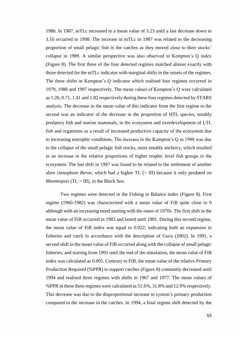
55
1986. In 1987, mTLc increased to a mean value of 3.23 until a last decrease down to
3.16 occurred in 1998. The increase in mTLc in 1987 was related to the decreasing
proportion of small pelagic fish in the catches as they moved close to their stocks’
collapse in 1989. A similar perspective was also observed in Kempton’s Q index
(Figure 8). The first three of the four detected regimes matched almost exactly with
those detected for the mTLc indicator with marginal shifts in the onsets of the regimes.
The three shifts in Kempton’s Q indicator which realised four regimes occurred in
1979, 1988 and 1997 respectively. The mean values of Kempton’s Q were calculated
as 1.26, 0.71, 1.41 and 1.82 respectively during these four regimes detected by STARS
analysis. The decrease in the mean value of this indicator from the first regime to the
second was an indicator of the decrease in the proportion of HTL species, notably
predatory fish and marine mammals, in the ecosystem and overdevelopment of LTL
fish and organisms as a result of increased productive capacity of the ecosystem due
to increasing eutrophic conditions. The increase in the Kempton’s Q in 1988 was due
to the collapse of the small pelagic fish stocks, most notably anchovy, which resulted
in an increase in the relative proportions of higher trophic level fish groups in the
ecosystem. The last shift in 1997 was found to be related to the settlement of another
alien ctenophore Beroe, which had a higher TL (> III) because it only predated on
Mnemiopsis (TL = III), in the Black Sea.
Two regimes were detected in the Fishing in Balance index (Figure 8). First
regime (1960-1982) was characterised with a mean value of FiB quite close to 0
although with an increasing trend starting with the onset of 1970s. The first shift in the
mean value of FiB occurred in 1983 and lasted until 1991. During this second regime,
the mean value of FiB index was equal to 0.022, indicating both an expansion in
fisheries and catch in accordance with the description of Gucu (2002). In 1991, a
second shift in the mean value of FiB occurred along with the collapse of small pelagic
fisheries, and starting from 1991 until the end of the simulation, the mean value of FiB
index was calculated as 0.005. Contrary to FiB, the mean value of the relative Primary
Production Required (%PPR) to support catches (Figure 8) constantly decreased until
1994 and realised three regimes with shifts in 1967 and 1977. The mean values of
%PPR in these three regimes were calculated as 51.6%, 31.8% and 12.9% respectively.
This decrease was due to the disproportional increase in system’s primary production
compared to the increase in the catches. In 1994, a final regime shift detected by the

56
STARS algorithm and the mean %PPR increased to 19% along with recuperating
fisheries.
Figure 8. The time-dynamic changes in the indicators (dots) and the regimes detected
(lines) by the STARS algorithm. Abbreviations are as follows: TST (Total System
Throughput), FCI (Finn’s Cycling Index), %PPR (relative Primary Production
Required to support catches), mTLc (mean trophic level of catch), and FiB (Fishing in
Balance). The TST, primary production, catch, and biomass properties are in gC m-2

57
y-1. FCI is percent of TST. Ascendency, overhead and %PPR are in percentages. Other
indicators are unitless. The x-axis denotes simulation years.
Considering ratios, although some inverse trends occurred during specific
years when catastrophic events like anchovy-Mnemiopsis shift occurred, the
proportion of large fish by weight in the ecosystem decreased after 1965 realising the
decrease in the mean trophic level of the catches observed throughout the simulation
(Figure 9).
Figure 9. Large fish by weight simulated by the time-dynamic model. Dots represent
the model simulation and line represents the regimes detected by the STARS analysis.
Considering ratios of fish groups (Figure 10), the consequences of fisheries
exploitation were also found to be evident. The ratio of piscivorous fish to forage and
other fish in the Black Sea had declined with time. The STARS algorithm detected two
regimes in these two ratios both of which separated by a shift in 1965. Further, the
ratio of demersal fish to pelagic fish increased during 1971 and decreased again in the
1994 showing the impact of fisheries exploitation on the ecosystem.
The ratio of opportunistic zooplankton (jellyfish and heterotrophic
dinoflagellates) to total zooplankton biomass increased in the early 1970s reaching up

58
to 55% of the whole zooplankton community in 1980s. This finding was also justified
by the in-situ observations (Shiganova et al., 2008). After 1994, this ratio decreased to
an extent so as to decrease the dominance of opportunistic zooplankton in the
zooplankton community.
Figure 10. The time-dynamic changes in the ratios (dots) and the regimes detected
(lines) by the STARS algorithm. The x-axis denotes simulation years.
The increasing enrichment in the Black Sea ecosystem was also delineated by
the biomass ratio of heterotrophic dinoflagellate Noctiluca to the sum of the biomasses
of Noctiluca and phytoplankton (Figure 11). Although there were significant
fluctuations, there was a general increasing trend in the ratio in accordance with the
increase in the primary production and total system throughput of the ecosystem
(Figure 8).
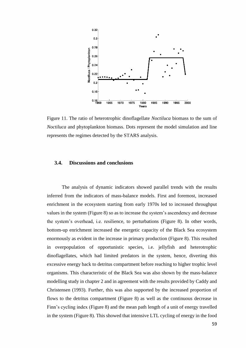
59
Figure 11. The ratio of heterotrophic dinoflagellate Noctiluca biomass to the sum of
Noctiluca and phytoplankton biomass. Dots represent the model simulation and line
represents the regimes detected by the STARS analysis.
3.4. Discussions and conclusions
The analysis of dynamic indicators showed parallel trends with the results
inferred from the indicators of mass-balance models. First and foremost, increased
enrichment in the ecosystem starting from early 1970s led to increased throughput
values in the system (Figure 8) so as to increase the system’s ascendency and decrease
the system’s overhead, i.e. resilience, to perturbations (Figure 8). In other words,
bottom-up enrichment increased the energetic capacity of the Black Sea ecosystem
enormously as evident in the increase in primary production (Figure 8). This resulted
in overpopulation of opportunistic species, i.e. jellyfish and heterotrophic
dinoflagellates, which had limited predators in the system, hence, diverting this
excessive energy back to detritus compartment before reaching to higher trophic level
organisms. This characteristic of the Black Sea was also shown by the mass-balance
modelling study in chapter 2 and in agreement with the results provided by Caddy and
Christensen (1993). Further, this was also supported by the increased proportion of
flows to the detritus compartment (Figure 8) as well as the continuous decrease in
Finn’s cycling index (Figure 8) and the mean path length of a unit of energy travelled
in the system (Figure 8). This showed that intensive LTL cycling of energy in the food

60
web due to over-proliferation of opportunistic organisms deprived the HTL groups,
i.e. fish, of significant resources from system’s production, which otherwise would be
shared across the upper trophic levels of the food web to support their biomass
development. Further, the increasing proportion of opportunistic zooplankton in the
total zooplankton community was a reason of this situation (Figure 10).
Second, fisheries played a structuring role on the ecosystem of the Black Sea.
The decreasing mTLc suggested that a “fishing down the food web” (Pauly et al.,
1998) effect had been realised in the ecosystem. This effect was also supported by the
decreasing ratio of piscivorous organisms (predatory fish and marine mammals) to
forage and other fish assemblages (Figure 10). By the end of 1960s, many of the higher
trophic level fish species had already been overexploited leading to the shift in 1965
detected by the STARS analysis, which was in accordance with the analysis of Oguz
(2007). This thinning-out (Petersen, 1903) of the Black Sea ecosystem’s fish
community was also reflected by the decreasing Kempton’s Q index from 1960s to the
end of 1970s. Kempton’s Q, which indicates the proportion of organisms in the
ecosystem with a trophic level equal to or higher than III, decreased significantly by
the end of 1970s (Figure 8).
The relative primary production required to support catches (%PPR) decreased
through the simulation period until its shift in 1994. However, at a first glance, the
%PPR would have been expected to increase in accordance with the increases detected
in the “Catch” and “FiB” indicators of the system when catches started to increase
significantly. Considering this decrease in the mean value of %PPR, it could be
concluded that the disproportionate increase in the system’s primary productivity
capacity far exceeded the increase in the catches. If the absolute PPR value was
considered (Figure 12), it was shown that the value of PPR increased in accordance
with the increasing catches. With the overexploitation of higher trophic level fish
species by the end of 1960s and with the onset of overenrichment as well as the
expansion of fishing fleet, the catches started to increase, however, the mean trophic
level of the catch was significantly lower compared to 1960s (as evident in the shift in
mTLc in 1967) because it consisted of mostly lower trophic level fish species like
small pelagic fish. Therefore, the %PPR decreased continuously until 1994 due to the
disproportionate increase in system’s primary production compared to the increase in
catches. In 1994, with the alleviating eutrophic conditions, a decreasing shift in the

61
mean value of %PPR occurred. After this year, the fisheries and the fish stocks
recovered; however, the catch did not reach to those levels of 1980s and the primary
productivity of the system was considerably constrained compared to the 1980s, hence,
an increase in the %PPR and a regime shift for this indicator were detected.
Figure 12. Primary Production Required (PPR) to sustain fisheries catches.
Considering the final status of the Black Sea ecosystem in the end of the
simulation period in 1999, it could be inferred that the ecosystem conditions in the
Black Sea was more degraded compared to the 1960s, however, in a better situation
than that observed during the 1970s and 1980s considering the above discussed
changes in the synthetic indicators and ratios. The most important factors that drove
these changes over time was the eutrophication and fisheries exploitation. As detected
in the primary production, the ecosystem experienced two shifts in 1978 and 1994.
The shift in 1978 was due to the onset of intensive eutrophication and the latter was
due to the alleviating eutrophic conditions and pollution in the Black Sea. The
consequences of this alleviation were evident in the shift observed in the non-edible
zooplankton to total zooplankton ratio towards the end of 1990s, which led to decrease
in the proportion of these opportunistic organisms among the total zooplankton
community. The timing of this shift in the zooplankton assemblage was also supported
by Shiganova et al. (2008) depending on in-situ sampling data and regarded as “a sign
of ecosystem rehabilitation at the zooplankton community level”.
62
4. CHAPTER: Translation of Ecopath with Ecosim into
FORTRAN 95/2003 language for coupling
4.1. Introduction
Since the very first steps taken by the founding father of ecology (Haeckel,
1866), ecosystem research has developed to become a challenging field of science with
the increasing understanding of the nonlinear interactions between the components that
make up an ecosystem. This had first led to the development of primitive “ecosystem”
models in the form of simple mathematical functions to represent prey-predator
relationships (Lotka, 1920; Volterra, 1926). Later with the advancement in the
computing technology during the second half of the 20th century, these mathematical
representations of individuals in the ecosystem started to be used to build up
mathematical models to represent multi-species interactions by coupling these
equations with one another. For a couple of decades, such models of biogeochemistry
and lower and higher trophic levels have been used in the marine environment with a
certain degree of success. Though useful for understanding fundamental interactions,
these representations of the ecosystems were short on explaining the holistic picture in
the marine environments they represented. This led to the necessity for building
integrated descriptions of food webs by coupling these models with one another in
order to form a complete ecosystem representation from the microbiological and
primary production processes up to fish assemblages and marine mammals through
schemes called End-to-End (E2E) models (Rose et al., 2010; Salihoglu et al., 2013).
This has been proven to be a challenging task (Fulton, 2010).
Hydrodynamic and biogeochemical models, which have been developed for
more than a couple of decades, have been used together to assess the interactions
between the biological and physical processes in the marine environment on the level
of lower trophic level processes. Parallel to these efforts, various comprehensive
models focusing on higher trophic level processes have been developed such as
Ecopath (Polovina, 1984; Christensen and Pauly, 1992), Ecosim (Walters et al., 1997;
2000), OSMOSE (Shin et al., 2004) and ATLANTIS (Fulton et al., 2011). Among
63
these tools, Ecopath with Ecosim (Christensen et al., 2005) was the most adopted tool
in marine ecosystems as an end-to-end model. However, though its success, EwE is
considered to be short on representing the nutrient cycle and lower trophic level
dynamics such as primary and secondary productions and focused on the
representation of life processes of fish species and other HTL organisms with annual
and multiannual development cycles. In the recent years, this shortcoming of EwE has
been tried to be remedied by utilising simple offline (Libralato and Solidoro, 2009)
and complicated online (Beecham et al., in prep.) linking methodologies with existing
models to a limited extent. However, these efforts has yet to be successful to the degree
that they could be recognised and widely adopted by ecosystem modellers because
until now these efforts either utilised only offline coupling and/or incorporated
complicated programming tricks far more sophisticated than the modelling itself. This
was the consequence of the fact that biogeochemical and hydrodynamic models were
mostly written FORTRAN whereas EwE was prescribed in Visual Basic.
Considering above mentioned complications, in this chapter of the thesis,
the first version of Ecopath with Ecosim translated into the FORTRAN language
was presented in the endeavour of providing a useful tool for directly
incorporating EwE as a module in existing biogeochemical models. Therefore, in
this chapter, the methodology used for the translation was explained and evidence of
the reliability of the code was provided by means of comparisons between standard
EwE 6 version and the EwE-FORTRAN using the Generic 37 model scenario, which
is distributed by the EwE 6 package, as a comparative test case. Further, the
FORTRAN version of the model explained in the subsequent sections was also used
for offline and one-way coupling with BIMS-ECO model for the analyses and testes
detailed in Chapter 5. By providing such a tool, it was believed that it will be useful
in expanding the application of the software either for coupling and/or analyses
by the interested scientific community, which have been hampered by the lack of
a FORTRAN version of the model until now.
64
4.2. Materials and Methods
The calculations in the Ecosim dynamic model were classified under four main
groups; i) nutrient calculations, ii) prey-predator calculations, iii) derivative function
calculations, and iv) integrator calculations, all of which were summarised in the
subsequent subsections.
4.2.1. Nutrient calculations
Ecosim dynamic model starts with initial state calculations for setting up the
initial conditions of state variables and parameters using basic input parameters of
Ecopath. As a first step, the total and free base nutrient concentrations, which are going
to drive the production of every state variable, are calculated as
𝑁𝑏𝑖𝑜𝑚𝑎𝑠𝑠 =∑𝐵𝑖𝐸
𝑛
𝑖
(6)
where 𝑁𝑏𝑖𝑜𝑚𝑎𝑠𝑠 is the biomass available in the system for the nutrient budget, i is the
group number, n equals to the number of state variables and 𝐵𝑖𝐸 is the Ecopath biomass
estimate of group i. Then total nutrient concentration (𝑁𝑡𝑜𝑡𝑎𝑙) is calculated as
𝑁𝑡𝑜𝑡𝑎𝑙 =𝑁𝑏𝑖𝑜𝑚𝑎𝑠𝑠
(1 − 𝑁𝐵𝑎𝑠𝑒𝐹𝑟𝑒𝑒𝑃𝑟𝑜𝑝) (7)
where 𝑁𝐵𝑎𝑠𝑒𝐹𝑟𝑒𝑒𝑃𝑟𝑜𝑝 is the base proportion of free nutrients, which equals to a value
close to unity. Hence, free nutrient concentration (𝑁𝑓𝑟𝑒𝑒) is estimated as
𝑁𝑓𝑟𝑒𝑒 = 𝑁𝑡𝑜𝑡𝑎𝑙 − 𝑁𝑏𝑖𝑜𝑚𝑎𝑠𝑠
(8)
and free base nutrient concentration (𝑁𝐹𝑟𝑒𝑒𝐵𝑎𝑠𝑒) equals
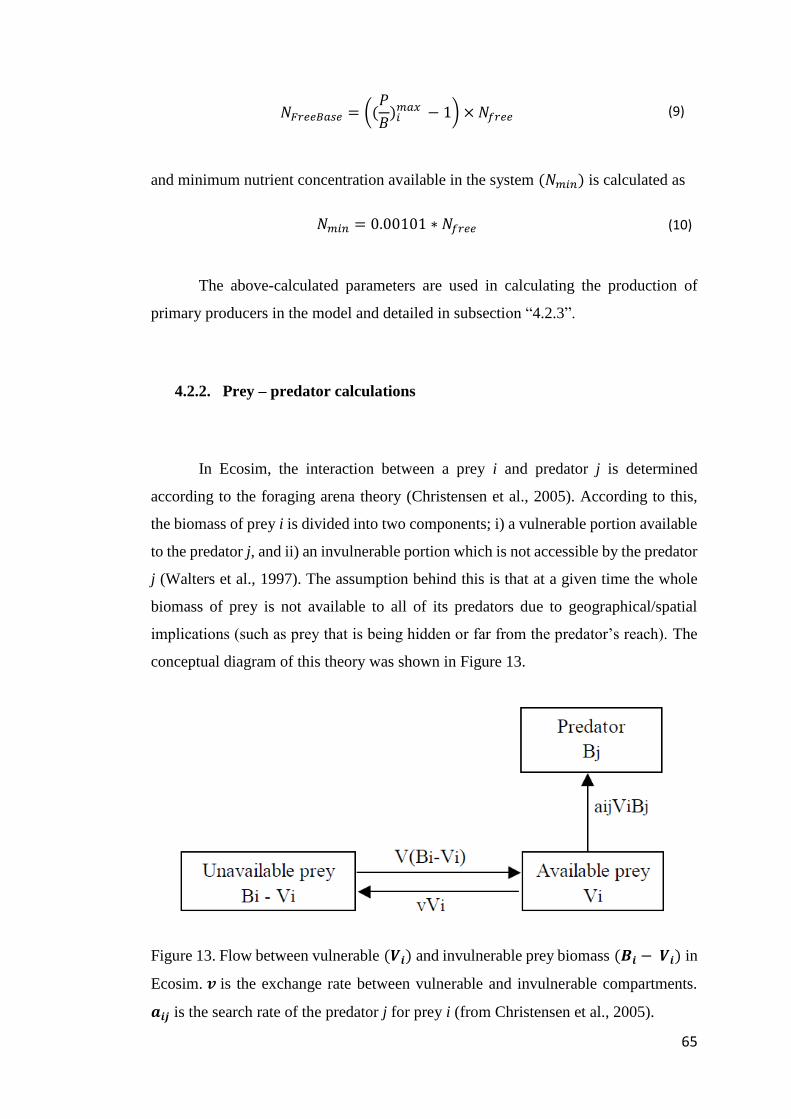
65
𝑁𝐹𝑟𝑒𝑒𝐵𝑎𝑠𝑒 = ((𝑃
𝐵)𝑖𝑚𝑎𝑥 − 1) × 𝑁𝑓𝑟𝑒𝑒 (9)
and minimum nutrient concentration available in the system (𝑁𝑚𝑖𝑛) is calculated as
𝑁𝑚𝑖𝑛 = 0.00101 ∗ 𝑁𝑓𝑟𝑒𝑒 (10)
The above-calculated parameters are used in calculating the production of
primary producers in the model and detailed in subsection “4.2.3”.
4.2.2. Prey – predator calculations
In Ecosim, the interaction between a prey i and predator j is determined
according to the foraging arena theory (Christensen et al., 2005). According to this,
the biomass of prey i is divided into two components; i) a vulnerable portion available
to the predator j, and ii) an invulnerable portion which is not accessible by the predator
j (Walters et al., 1997). The assumption behind this is that at a given time the whole
biomass of prey is not available to all of its predators due to geographical/spatial
implications (such as prey that is being hidden or far from the predator’s reach). The
conceptual diagram of this theory was shown in Figure 13.
Figure 13. Flow between vulnerable (𝑽𝒊) and invulnerable prey biomass (𝑩𝒊 − 𝑽𝒊) in
Ecosim. 𝒗 is the exchange rate between vulnerable and invulnerable compartments.
𝒂𝒊𝒋 is the search rate of the predator j for prey i (from Christensen et al., 2005).
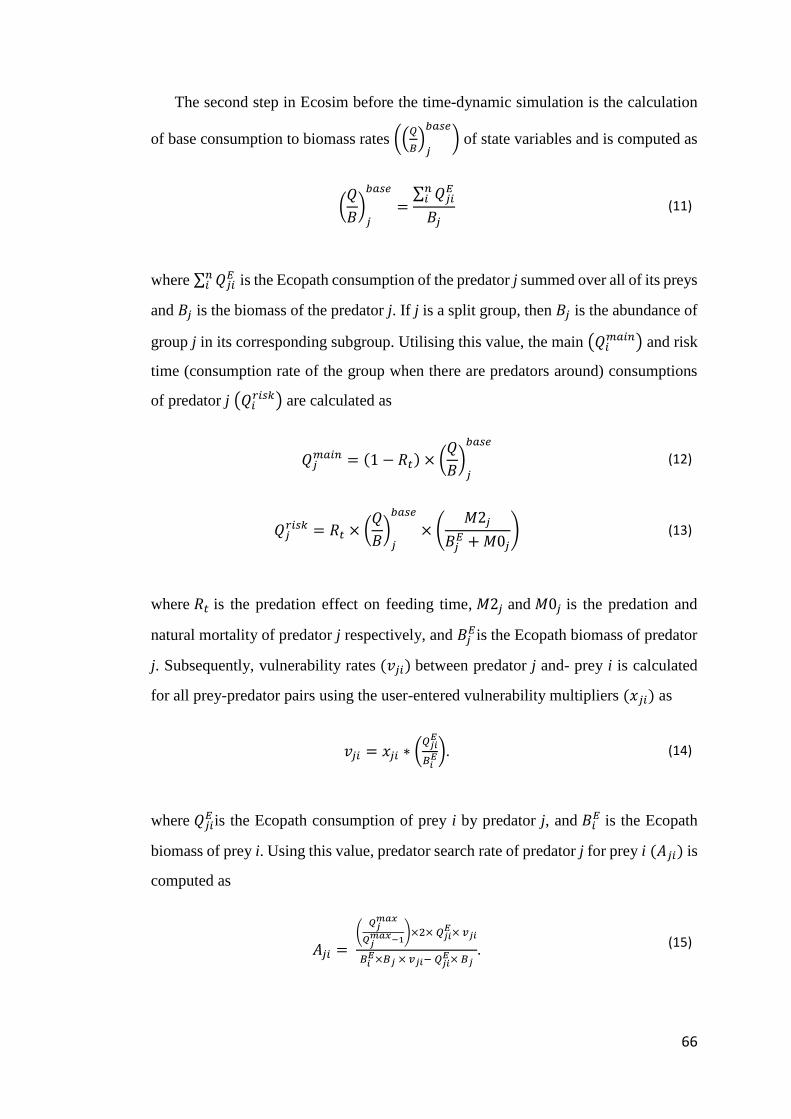
66
The second step in Ecosim before the time-dynamic simulation is the calculation
of base consumption to biomass rates ((𝑄
𝐵)𝑗
𝑏𝑎𝑠𝑒
) of state variables and is computed as
(𝑄
𝐵)𝑗
𝑏𝑎𝑠𝑒
=∑ 𝑄𝑗𝑖
𝐸𝑛𝑖
𝐵𝑗 (11)
where ∑ 𝑄𝑗𝑖𝐸𝑛
𝑖 is the Ecopath consumption of the predator j summed over all of its preys
and 𝐵𝑗 is the biomass of the predator j. If j is a split group, then 𝐵𝑗 is the abundance of
group j in its corresponding subgroup. Utilising this value, the main (𝑄𝑖𝑚𝑎𝑖𝑛) and risk
time (consumption rate of the group when there are predators around) consumptions
of predator j (𝑄𝑖𝑟𝑖𝑠𝑘) are calculated as
𝑄𝑗𝑚𝑎𝑖𝑛 = (1 − 𝑅𝑡) × (
𝑄
𝐵)𝑗
𝑏𝑎𝑠𝑒
(12)
𝑄𝑗𝑟𝑖𝑠𝑘 = 𝑅𝑡 × (
𝑄
𝐵)𝑗
𝑏𝑎𝑠𝑒
× (𝑀2𝑗
𝐵𝑗𝐸 +𝑀0𝑗
) (13)
where 𝑅𝑡 is the predation effect on feeding time, 𝑀2𝑗 and 𝑀0𝑗 is the predation and
natural mortality of predator j respectively, and 𝐵𝑗𝐸is the Ecopath biomass of predator
j. Subsequently, vulnerability rates (𝑣𝑗𝑖) between predator j and- prey i is calculated
for all prey-predator pairs using the user-entered vulnerability multipliers (𝑥𝑗𝑖) as
𝑣𝑗𝑖 = 𝑥𝑗𝑖 ∗ (𝑄𝑗𝑖𝐸
𝐵𝑖𝐸). (14)
where 𝑄𝑗𝑖𝐸 is the Ecopath consumption of prey i by predator j, and 𝐵𝑖
𝐸 is the Ecopath
biomass of prey i. Using this value, predator search rate of predator j for prey i (𝐴𝑗𝑖) is
computed as
𝐴𝑗𝑖 = (𝑄𝑗𝑚𝑎𝑥
𝑄𝑗𝑚𝑎𝑥−1
)×2× 𝑄𝑗𝑖𝐸× 𝑣𝑗𝑖
𝐵𝑖𝐸×𝐵𝑗 × 𝑣𝑗𝑖− 𝑄𝑗𝑖
𝐸× 𝐵𝑗. (15)

67
where 𝑄𝑗𝑚𝑎𝑥 is the maximum relative consumption of predator j and 𝐵𝑗 is the biomass
of predator j at time 0. The relative prey switching parameter (𝑇𝑗𝑅𝑒𝑙𝑎𝑆𝑤𝑖𝑡𝑐ℎ) of predator
j for prey i at each simulation time step is calculated considering the base prey
switching parameter (𝑇𝑗𝐵𝑎𝑠𝑒𝑇𝑖𝑚𝑒𝑆𝑤𝑖𝑡𝑐ℎ) of predator j, which is calculated using
Ecopath values, as
𝑇𝑗𝐵𝑎𝑠𝑒𝑇𝑖𝑚𝑒𝑆𝑤𝑖𝑡𝑐ℎ =
𝐴𝑗𝑖 × (𝐵𝑖𝐸)𝑆𝑃𝑗
∑ (𝐴𝑗𝑖 ×𝑛𝑖 (𝐵𝑖
𝐸)𝑆𝑃𝑗) (16)
𝑇𝑗𝑅𝑒𝑙𝑎𝑆𝑤𝑖𝑡𝑐ℎ =
𝐴𝑗𝑖 × (𝐵𝑖(𝑡))𝑆𝑃𝑗
∑ (𝐴𝑗𝑖 ×𝑛𝑖 (𝐵𝑖(𝑡))
𝑆𝑃𝑗)
𝑇𝑗𝐵𝑎𝑠𝑒𝑇𝑖𝑚𝑒𝑆𝑤𝑖𝑡𝑐ℎ
(17)
where 𝑆𝑃𝑗 is the user-entered switching power parameter of predator j in the Group
Info tab of Ecosim and 𝐵𝑖(𝑡) is the biomass of prey i at simulation time t. From this,
vulnerable pool of biomass of prey i (𝑉𝑖) is calculated as
𝑉𝑖 = (𝑥𝑗𝑖 − 1) ∗ (𝑄𝑗
2∗𝑣𝑗𝑖). (18)
where 𝑄𝑗 is the consumption of predator j in its corresponding foraging arena and
calculated by multiplying the Ecopath consumption of predator j of prey i with the
feeding time, which is a relative indicator of time spent by predator j for seeking prey
i. Hence, feeding time ranges between 0 and 1 and depends on the concentration of the
predators of j present in the system at time step t.

68
4.2.3. Derivative Function Calculations
The state equation of a variable i is
𝑑𝑖
𝑑𝑡= 𝑓(𝐵𝑖) + 𝐼𝑖 −∑𝑄𝑗𝑖(𝑡) − 𝑀0𝑖 − 𝐹𝑖, − 𝐸𝑖
𝑛
𝑗
(19)
where 𝑓(𝐵𝑖) is production as a function of biomass, 𝐼𝑖 is emigration, 𝑄𝑗𝑖 is
consumption of i by predator j, 𝑀0𝑖 is natural mortality, 𝐹𝑖 is the fishing mortality and
𝐸𝑖 is the emigration. If i is a primary producer, 𝑓(𝐵𝑖) equals to
𝑓(𝐵𝑖) = 𝑅𝑖𝑚𝑎𝑥 ∗ 𝑁𝑓𝑟𝑒𝑒
𝑁𝑓𝑟𝑒𝑒 + 𝑁𝐹𝑟𝑒𝑒𝐵𝑎𝑠𝑒∗
(𝑃𝐵)𝑖
𝐸
∗ 𝑅𝑖𝑚𝑎𝑥
1 + 𝐵𝑖(𝑡) ∗ (((𝑃𝐵)𝑖
𝐸
∗ 𝑅𝑖𝑚𝑎𝑥
(𝑃𝐵)𝑖
𝐸
− 1
)/ 𝐵𝑖𝐸)
∗ 𝐹(𝑡) ∗ 𝐵𝑖(𝑡) (20)
where (𝑃
𝐵)𝑖
𝐸
is the Ecopath production to biomass ratio, 𝐵𝑖𝐸 is the Ecopath biomass of
producer, 𝐵𝑖(𝑡) is the biomass of producer at time t, 𝑅𝑖𝑚𝑎𝑥 is maximum relative
production to biomass ratio, 𝑁𝑓𝑟𝑒𝑒is total amount of free nutrients and 𝑁𝐹𝑟𝑒𝑒𝐵𝑎𝑠𝑒 is the
free base nutrient concentration.
For consumer groups the state equation becomes in the form of
𝑑𝑖
𝑑𝑡= 𝑔𝑖
𝑚𝑎𝑥 ∗∑𝑄𝑖𝑗(𝑡)
𝑛
𝑖
+ 𝐼𝑖 −∑𝑄𝑗𝑖(𝑡) − 𝑀0𝑖 − 𝐹𝑖, − 𝐸𝑖
𝑛
𝑗
(21)
where 𝑔𝑖𝑚𝑎𝑥 is the maximum growth efficiency of group i, 𝑄𝑖𝑗(𝑡) is the consumption
of group i on group j at simulation time t, 𝑄𝑗𝑖 is the consumption of group I by its
predator j, and the rest of the parameters are identical to those of the state equation for
primary producers. 𝑔𝑖𝑚𝑎𝑥 is estimated as

69
𝑔𝑖𝑚𝑎𝑥 = (
𝑃
𝑄)𝑖
𝐸
(22)
where (𝑃
𝑄)𝑖
𝐸
is the Ecopath production to consumption ratio of group i. The
consumption of predator j on prey i (𝑄𝑗𝑖) is calculated as
𝑄𝑗𝑖 = ∑𝐴𝑗𝑒𝑓𝑓
∗ 𝑉𝑖
0.5 ∗ (1 + 𝐻𝑗 ∗ 𝐴𝑗𝑒𝑓𝑓
∗ 𝑉𝑖) + 0.5 ∗ (𝑄𝑗𝑚𝑎𝑥
𝑄𝑗𝑚𝑎𝑥 − 1
)
∗ 𝐵𝑗(𝑡)
𝑛
𝑖
(23)
where 𝐴𝑗𝑒𝑓𝑓
is the effective search rate of predator j and 𝐻𝑗 is the handling time of the
predator. 𝐻𝑗 is calculated as
𝐻𝑗 =𝐵𝑗
𝑄𝑗𝑚𝑎𝑥 ∗ 𝐵𝑗
𝐸 ∗ (𝑄𝐵)𝑗
𝐸 (24)
where 𝐵𝑗 is the biomass of predator j at time 0, 𝐵𝑗𝐸is the Ecopath calculated biomass
of predator j. (𝑄
𝐵)𝑗
𝐸
is the Ecopath consumption to biomass ratio of predator j. And 𝐴𝑗𝑒𝑓𝑓
is calculated as
𝐴𝑗𝑒𝑓𝑓
=
(𝑄𝑗𝑚𝑎𝑥
𝑄𝑗𝑚𝑎𝑥 − 1
) ∗ 𝑄𝑗𝑖
𝑉𝑖 ∗ 𝐵𝑗∗ 𝐹𝑗
𝑡𝑖𝑚𝑒 ∗ 𝑇𝑗𝑟𝑒𝑙𝑎𝑠𝑤𝑖𝑡𝑐ℎ
(25)
where 𝐹𝑗𝑡𝑖𝑚𝑒is the feeding time of predator j, which is equal to unity at simulation time
0. And (𝑉𝑖) is the final vulnerable biomass of prey i and is equal to
𝑉𝑖 = 𝑉𝑗𝑖𝑒𝑓𝑓
𝑣𝑗𝑖 + 𝑉𝑗𝑖𝑒𝑓𝑓 +
(
𝐴𝑗
𝑒𝑓𝑓∗ 𝐵𝑗(𝑡)
0.5 ∗ (1 + 𝐻𝑗 ∗ 𝐴𝑗𝑒𝑓𝑓∗ 𝑉𝑖
∗) + 0.5 ∗ (𝑄𝑗𝑚𝑎𝑥
𝑄𝑗𝑚𝑎𝑥 − 1
)
)
∗ 𝐵𝑖(𝑡)
(26)
where (𝑉𝑖∗) is the initial vulnerable biomass estimate of prey i and equals to
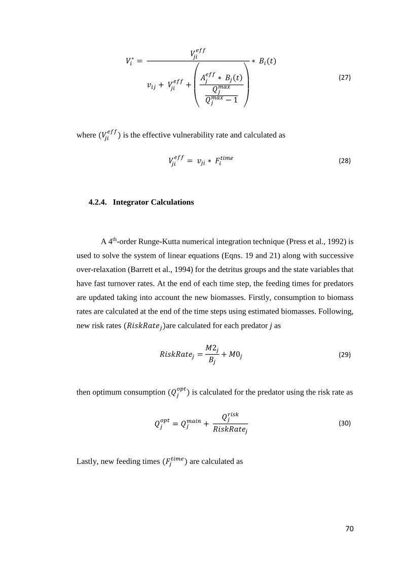
70
𝑉𝑖∗ =
𝑉𝑗𝑖𝑒𝑓𝑓
𝑣𝑖𝑗 + 𝑉𝑗𝑖𝑒𝑓𝑓
+
(
𝐴𝑗
𝑒𝑓𝑓∗ 𝐵𝑗(𝑡)
𝑄𝑗𝑚𝑎𝑥
𝑄𝑗𝑚𝑎𝑥 − 1
)
∗ 𝐵𝑖(𝑡)
(27)
where (𝑉𝑗𝑖𝑒𝑓𝑓) is the effective vulnerability rate and calculated as
𝑉𝑗𝑖𝑒𝑓𝑓
= 𝑣𝑗𝑖 ∗ 𝐹𝑖𝑡𝑖𝑚𝑒 (28)
4.2.4. Integrator Calculations
A 4th-order Runge-Kutta numerical integration technique (Press et al., 1992) is
used to solve the system of linear equations (Eqns. 19 and 21) along with successive
over-relaxation (Barrett et al., 1994) for the detritus groups and the state variables that
have fast turnover rates. At the end of each time step, the feeding times for predators
are updated taking into account the new biomasses. Firstly, consumption to biomass
rates are calculated at the end of the time steps using estimated biomasses. Following,
new risk rates (𝑅𝑖𝑠𝑘𝑅𝑎𝑡𝑒𝑗)are calculated for each predator j as
𝑅𝑖𝑠𝑘𝑅𝑎𝑡𝑒𝑗 =𝑀2𝑗
𝐵𝑗+𝑀0𝑗 (29)
then optimum consumption (𝑄𝑗𝑜𝑝𝑡) is calculated for the predator using the risk rate as
𝑄𝑗𝑜𝑝𝑡 = 𝑄𝑗
𝑚𝑎𝑖𝑛 + 𝑄𝑗𝑟𝑖𝑠𝑘
𝑅𝑖𝑠𝑘𝑅𝑎𝑡𝑒𝑗 (30)
Lastly, new feeding times (𝐹𝑗𝑡𝑖𝑚𝑒) are calculated as

71
𝐹𝑗𝑡𝑖𝑚𝑒 = 0.1 + 0.9 ∗ 𝐹𝑗
𝑡𝑖𝑚𝑒 ∗
(
1 − 𝐹𝑗𝑡𝑖𝑚𝑒𝐴𝑑𝑗𝑢𝑠𝑡𝑒𝑑
+𝐹𝑗𝑡𝑖𝑚𝑒𝐴𝑑𝑗𝑢𝑠𝑡𝑒𝑑
∗ 𝑄𝑗𝑜𝑝𝑡
(𝑄𝐵)𝑗
𝑡
)
(31)
where 𝐹𝑗𝑡𝑖𝑚𝑒𝐴𝑑𝑗𝑢𝑠𝑡𝑒𝑑
is the user-entered feeding time adjustment rate in the Group Info
tab of Ecosim.
4.2.5. The Skill Assessment of EwE-FORTRAN
The skill of the FORTRAN transcribed version of Ecopath with Ecosim (EwE-
FORTRAN) was tested with the sample hypothetical model named “Generic 37”,
which is distributed with the Ecopath with Ecosim 6 model package. The “Generic 37”
model was run both with EwE 6 and EwE-FORTRAN programs and the results of the
simulated biomasses of state variables were compared.
4.3. Results and Discussions
The residuals of the state variables calculated from the comparison of the
simulations of Generic 37 model with EwE 6 and EwE-FORTRAN models justified
that the FORTRAN version of the model had skill to reproduce the results of the EwE
6 for the Generic 37 model scenario (Figure 14). The residuals ranged between the
orders of 10-6 and 10-4, and the maximum error was found to be on the order of 10-4
for groups feeding on detritus (groups 6, 8, 16, 17, 24, 27, 29, 31) and the detritus
group (group 37). This suggested that detritus dynamics might not have been correctly
formulated in the FORTRAN version of the model and should be further refined.
However, the magnitude of the misfits concluded that EwE-FORTRAN was capable
of being used in coupling with biogeochemical models as detailed in chapter 5 without
introducing significant sources of error to the resulting model scheme.

72
Figure 14. The residuals of the simulated biomasses of the state variables showing the degree of misfit between EwE 6 and EwE-FORTRAN
model simulation outputs for the Generic 37 model.

73
5. CHAPTER: Scenarios on future ecosystem functioning under
changing climatological and fisheries conditions
5.1. Introduction
For more than a decade, end-to-end models have increased the understanding
of ecosystems at a broader scale including the feedbacks and interactions between
coupled physical, chemical and biological systems (Fulton, 2010; Shin et al., 2010a;
Rose et al., 2010; Travers et al., 2007). These models were considered as integrated
ecosystem models that included ecosystem components from primary producers up to
top predatory organisms and their interactions with the abiotic environment (Fulton,
2010). With such models, not only were the impacts of anthropogenic activities such
as fishing and pollution examined, but long-term effects of climate variability and its
consequences on the ecosystem scale could have also been investigated.
Ecopath with Ecosim model could be regarded as an end-to-end representation
of the marine ecosystem from primary producers to top predators such as fish, marine
mammals and even sea birds. Because the primary motivation in developing the EwE
model focused on fisheries, the life history of fish groups was formulated in detail,
whereas, the lower trophic level groups with relatively higher rate of turnover
remained weakly prescribed. Further, concerning the complicated biogeochemical
processes that take part in a given system’s primary and secondary productivity
processes under the strong influence of physical drivers such as mixing, temperature,
and light, the lower trophic level representation of EwE could be considered as rather
simplistic (see section 4.2.1). It did not incorporate these processes explicitly,
however, implicit representations of their effects on the biogeochemical processes
such as the production capacity of primary producers were represented through
implementation of forcing and mediation functions. Therefore, for the sake of better
representation of these aforementioned processes and their impacts, the EwE model
was required to be coupled with advanced biogeochemical models which functioned
in conjunction with hydrodynamic models.
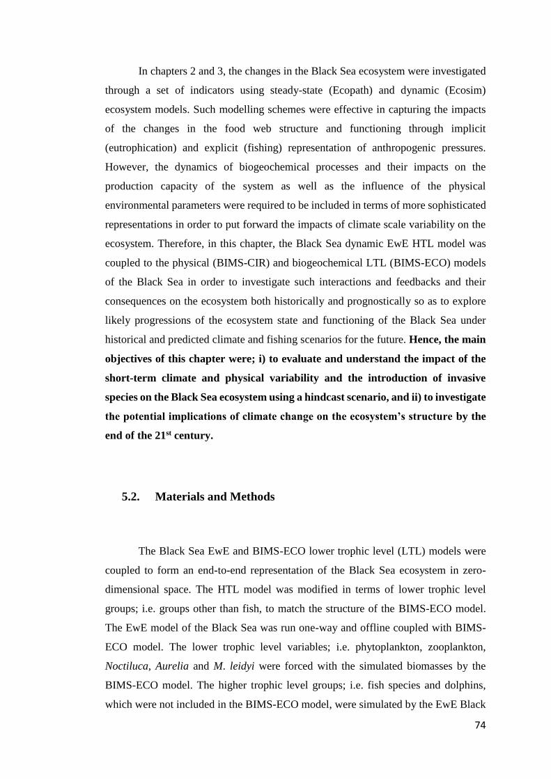
74
In chapters 2 and 3, the changes in the Black Sea ecosystem were investigated
through a set of indicators using steady-state (Ecopath) and dynamic (Ecosim)
ecosystem models. Such modelling schemes were effective in capturing the impacts
of the changes in the food web structure and functioning through implicit
(eutrophication) and explicit (fishing) representation of anthropogenic pressures.
However, the dynamics of biogeochemical processes and their impacts on the
production capacity of the system as well as the influence of the physical
environmental parameters were required to be included in terms of more sophisticated
representations in order to put forward the impacts of climate scale variability on the
ecosystem. Therefore, in this chapter, the Black Sea dynamic EwE HTL model was
coupled to the physical (BIMS-CIR) and biogeochemical LTL (BIMS-ECO) models
of the Black Sea in order to investigate such interactions and feedbacks and their
consequences on the ecosystem both historically and prognostically so as to explore
likely progressions of the ecosystem state and functioning of the Black Sea under
historical and predicted climate and fishing scenarios for the future. Hence, the main
objectives of this chapter were; i) to evaluate and understand the impact of the
short-term climate and physical variability and the introduction of invasive
species on the Black Sea ecosystem using a hindcast scenario, and ii) to investigate
the potential implications of climate change on the ecosystem’s structure by the
end of the 21st century.
5.2. Materials and Methods
The Black Sea EwE and BIMS-ECO lower trophic level (LTL) models were
coupled to form an end-to-end representation of the Black Sea ecosystem in zero-
dimensional space. The HTL model was modified in terms of lower trophic level
groups; i.e. groups other than fish, to match the structure of the BIMS-ECO model.
The EwE model of the Black Sea was run one-way and offline coupled with BIMS-
ECO model. The lower trophic level variables; i.e. phytoplankton, zooplankton,
Noctiluca, Aurelia and M. leidyi were forced with the simulated biomasses by the
BIMS-ECO model. The higher trophic level groups; i.e. fish species and dolphins,
which were not included in the BIMS-ECO model, were simulated by the EwE Black

75
Sea model. The resulting scheme of the one-way offline coupled model was shown in
Figure 15.
Figure 15. Coupled Black Sea model scheme. Light-grey boxes represent BIMS-ECO
model compartments and orange boxes represent EwE Black Sea model
compartments. Arrows indicate flows in terms of prey-predator interactions.
5.2.1. The Hydrodynamic and LTL Biogeochemical Model
The hydrodynamic model was a modified version of the sigma coordinate, free
surface Princeton Ocean Model (POM; Blumberg and Mellor, 1987). The model
domain incorporated the entire Black Sea (41°S - 46°N, 28°E - 41.5°E) excluding the
Azov Sea. It consisted of a 0.1o x 0.0625o resolution Arakawa C-type of horizontal grid

76
and a 26-level vertical grid. The sigma levels were compressed at the surface and
bottom boundary layers. The maximum depth of the model domain was 2200 m.
Considering that the Black Sea is a semi-enclosed sea, the lateral boundary conditions
were no-slip and zero-heat, and salt fluxes were prescribed everywhere in the whole
domain except the Bosphorus and Kerch straits as well as the mouths of the eight
largest rivers draining into the Black Sea (Danube, Dniester, Dnieper, Inguri, Rioni,
Yesilirmak, Kizilirmak, and Sakarya). At the mouths of the rivers and straits, boundary
conditions of temperature and salinity were prescribed as inflow conditions. Diffusive
heat and salt fluxes were set to nil in the straits outflow points (Cannaby et al., 2012).
The biogeochemical ecosystem model used in this study was the BIMS-ECO
model based on the 1D model by Oguz et al. (2001). The model had 12 state variables
that included two phytoplankton groups, small and large phytoplankton representing
flagellates and diatoms respectively, micro- (< 0.2 mm, Zs) and mesozooplankton (>
0.2-2 mm, Zl), bacterioplankton (B), labile pelagic detritus (D), DON, nitrate (N),
ammonium (A), as well as the opportunistic heterotrophic dinoflagellate Noctiluca
scintillans (Zn) and the gelatinous carnivores Aurelia aurita (Za) and Mnemiopsis
leidyi (Zm) (Figure 16).
Figure 16. BIMS-ECO lower trophic level model structure (from Oguz et al., 2001).
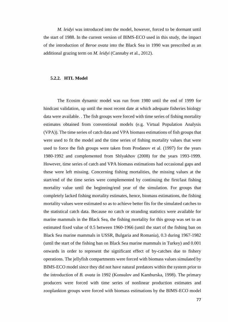
77
M. leidyi was introduced into the model, however, forced to be dormant until
the start of 1988. In the current version of BIMS-ECO used in this study, the impact
of the introduction of Beroe ovata into the Black Sea in 1990 was prescribed as an
additional grazing term on M. leidyi (Cannaby et al., 2012).
5.2.2. HTL Model
The Ecosim dynamic model was run from 1980 until the end of 1999 for
hindcast validation, up until the most recent date at which adequate fisheries biology
data were available. . The fish groups were forced with time series of fishing mortality
estimates obtained from conventional models (e.g. Virtual Population Analysis
(VPA)). The time series of catch data and VPA biomass estimations of fish groups that
were used to fit the model and the time series of fishing mortality values that were
used to force the fish groups were taken from Prodanov et al. (1997) for the years
1980-1992 and complemented from Shlyakhov (2008) for the years 1993-1999.
However, time series of catch and VPA biomass estimations had occasional gaps and
these were left missing. Concerning fishing mortalities, the missing values at the
start/end of the time series were complemented by continuing the first/last fishing
mortality value until the beginning/end year of the simulation. For groups that
completely lacked fishing mortality estimates, hence, biomass estimations, the fishing
mortality values were estimated so as to achieve better fits for the simulated catches to
the statistical catch data. Because no catch or stranding statistics were available for
marine mammals in the Black Sea, the fishing mortality for this group was set to an
estimated fixed value of 0.5 between 1960-1966 (until the start of the fishing ban on
Black Sea marine mammals in USSR, Bulgaria and Romania), 0.3 during 1967-1982
(until the start of the fishing ban on Black Sea marine mammals in Turkey) and 0.001
onwards in order to represent the significant effect of by-catches due to fishery
operations. The jellyfish compartments were forced with biomass values simulated by
BIMS-ECO model since they did not have natural predators within the system prior to
the introduction of B. ovata in 1992 (Konsulov and Kamburska, 1998). The primary
producers were forced with time series of nonlinear production estimates and
zooplankton groups were forced with biomass estimations by the BIMS-ECO model

78
during the simulation period. The time series of catch data and stock assessments of
other models such as VPA were used as a measure for the model fitting. The model
was calibrated utilising vulnerability (half-saturation) settings of the functional groups
as well as Monte-Carlo style parameter search routine for the mass-balance Ecopath
model. For biomass and catch estimates simulated by the EwE model, the goodness of
fit measures were the weighted sum of squared deviations (SS, Mood et al., 1974) of
log biomasses/catches from the log predicted biomasses and/or catches and Akaike
Information Criterion (AIC; Akaike, 1974). For phytoplankton groups, the same
measure of goodness of fit was calculated against the in-situ time series data from
which biomass predictions were calculated. There were 36 time series consisting of
in-situ catch and biomass measurements and statistical catch data which were used to
fit the model (for more details see section 3.2).
5.2.3. Scenarios
One hindcast scenario entitled Present Day (PD) was used by means of the
BIMS-CIR hydrodynamic model. The PD scenario was run for 20 years from 1980
until the end of 1999. Surface forcing was prescribed using 6-hourly fields of wind
stress, fresh water fluxes (evaporation, convective precipitation and large-scale
precipitation), and radiation fields (surface shortwave radiation, surface long-wave
radiation, evaporative heat flux, and convective heat flux). The PD scenario was forced
with the data extracted from Institut Pierre Simon Laplace (IPSL) Climate Model 4
(CM4) Ocean Atmosphere Global Circulation Model (OA-GCM) (Marti et al., 2006).
Further, one climate forced simulation (A1B) was run from 2080 until the end of 2099.
For this simulation, the model setup, initial conditions and river inputs were identical
to the end of the control simulation. The A1B scenario was evaluated and compared
against PD scenario on the basis of fractional change in the multiannual simulated
model outputs of the state variables. For any given state variable i, the fractional
change (fc) was calculated as

79
𝑓𝑐𝑖 =𝐵𝑖𝐴1𝐵𝐵𝑖𝑃𝐷
− 1 (32)
where 𝐵𝑖𝐴1𝐵and 𝐵𝑖𝑃𝐷were the average biomass of i over the whole simulation periods
of A1B and PD respectively. In order to test any given fractional change of state
variable i was statistically significant, a Kruskal-Wallis non-parametric 1-way
ANOVA test (Kruskal and Wallis, 1952) was applied to the model simulated time
series biomass values of the state variables.
The progressions in the fish community structure under 50% increased and
decreased fishing mortality levels for all fish groups were investigated in section 5.3.5
using the present day (PD) scenario. Furthermore, the sensitivity of the Black Sea
ecosystem to various fishing and primary productivity conditions was also explored
by means of six different scenarios focusing on the anchovy-Mnemiopsis shift using
the PD simulation in order to investigate the underlying causalities of the incident
(Table 19).
Table 19. Fishing scenarios used to explore the causalities of anchovy-Mnemiopsis
shift under different combinations of changing fishing mortality levels on the anchovy
stocks and alternating primary production and food web conditions.
Scenario Explanation
Scen. 1 Fmsy (Fishing mortality (F) required to
obtain Maximum Sustainable Yield (MSY))
value forced on anchovy stocks
Scen. 2 Fmsy value forced on anchovy stocks in
combination with invariant primary
production equal to the year of 1980
throughout the simulation period
Scen. 3 Fmsy value forced on anchovy stocks along
with no Mnemiopsis and Beroe introduction
to the food web

80
Scen. 4 Fmsy value forced on anchovy stocks along
with invariant primary production equal to
the year of 1980 throughout the simulation
period and no Mnemiopsis and Beroe
introduction to the food web
Scen. 5 Status quo (PD) fishing mortality values
applied on anchovy stock along with no
Mnemiopsis and Beroe introduction to the
food web
Scen. 6 Status quo (PD) fishing mortality values
applied on anchovy stock along with
invariant primary production equal to the
year of 1980 throughout the simulation
period
5.3. Results
5.3.1. Evaluation of Hindcast Model Results
The sum of squared deviations (SS) for 36 time series and AIC score for 72
data points were calculated as 164 and 475 respectively. Considering that the time
series had gaps for most demersal species; i.e. whiting, turbot, and spiny dogfish; and
some fish species such as bonito, bluefish, Atlantic mackerel, and red mullet did not
have any stock estimates but only catch statistics, the SS and AIC values could be
evaluated as the model had a good fit and medium uncertainty (Figure 17 and Figure
18).

81
Figure 17. PD run: Simulated biomass changes (solid lines) of the model
compartments and their degree of agreement with Virtual Population Analysis (VPA)
estimates (dots) for fish compartments. The y-axis shows biomass in gC m-2 and the
x-axis shows simulation years.

82
Figure 18. PD run: Simulated yield changes (solid lines) of the model compartments
and their degree of agreement with statistical catch data (dots) in the Black Sea. The
y-axis shows biomass in gC m-2 and the x-axis shows simulation years.
5.3.2. Changes in LTL
The annual mean depth-integrated basin-averaged primary production in the
A1B scenario was simulated to increase significantly compared to the PD scenario
according to the Kruskal-Wallis test (p < 0.05) and calculated to be 5% higher (mean
206 mgC m-2 d-1) than the PD scenario reflecting the impact of changed circulation
patterns in the A1B scenario due to the basin-wide 3 ºC temperature increase (Figure
19).
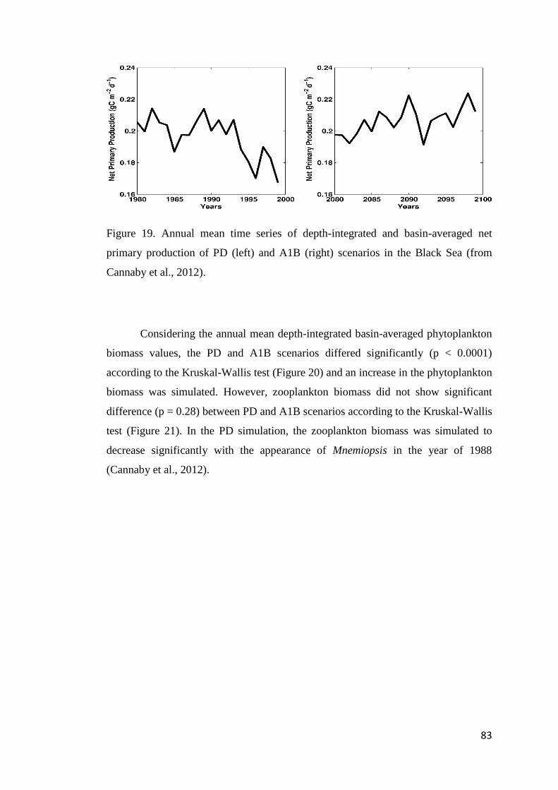
83
Figure 19. Annual mean time series of depth-integrated and basin-averaged net
primary production of PD (left) and A1B (right) scenarios in the Black Sea (from
Cannaby et al., 2012).
Considering the annual mean depth-integrated basin-averaged phytoplankton
biomass values, the PD and A1B scenarios differed significantly (p < 0.0001)
according to the Kruskal-Wallis test (Figure 20) and an increase in the phytoplankton
biomass was simulated. However, zooplankton biomass did not show significant
difference (p = 0.28) between PD and A1B scenarios according to the Kruskal-Wallis
test (Figure 21). In the PD simulation, the zooplankton biomass was simulated to
decrease significantly with the appearance of Mnemiopsis in the year of 1988
(Cannaby et al., 2012).

84
Figure 20. Annual mean time series of depth-integrated and basin-averaged
phytoplankton biomass of PD (left) and A1B (right) scenarios in the Black Sea (from
Cannaby et al., 2012).
Figure 21. Annual mean time series of depth-integrated and basin-averaged
zooplankton biomass of PD (left) and A1B (right) scenarios in the Black Sea (from
Cannaby et al., 2012).
Concerning the biomass variations of Aurelia, although a significant difference
was observed considering the minimum and maximum values, the 20-year biomass
fluctuations did not show significant difference between PD and A1B scenarios
according to the Kruskal-Wallis test (p = 0.3) (Figure 22).

85
Figure 22. Annual mean time series of depth-integrated and basin-averaged Aurelia
biomass of PD (left) and A1B (right) scenarios in the Black Sea (from Cannaby et al.,
2012).
Contrary to Aurelia’s, the biomass of Mnemiopsis, however, showed
significant difference between PD and A1B scenarios according to the Kruskal-Wallis
test (p = 0.001) (Figure 23).
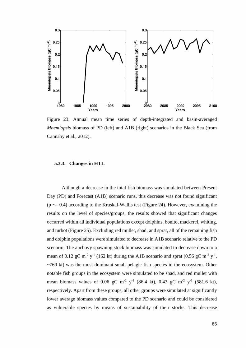
86
Figure 23. Annual mean time series of depth-integrated and basin-averaged
Mnemiopsis biomass of PD (left) and A1B (right) scenarios in the Black Sea (from
Cannaby et al., 2012).
5.3.3. Changes in HTL
Although a decrease in the total fish biomass was simulated between Present
Day (PD) and Forecast (A1B) scenario runs, this decrease was not found significant
(p ~= 0.4) according to the Kruskal-Wallis test (Figure 24). However, examining the
results on the level of species/groups, the results showed that significant changes
occurred within all individual populations except dolphins, bonito, mackerel, whiting,
and turbot (Figure 25). Excluding red mullet, shad, and sprat, all of the remaining fish
and dolphin populations were simulated to decrease in A1B scenario relative to the PD
scenario. The anchovy spawning stock biomass was simulated to decrease down to a
mean of 0.12 gC m-2 y-1 (162 kt) during the A1B scenario and sprat (0.56 gC m-2 y-1,
~760 kt) was the most dominant small pelagic fish species in the ecosystem. Other
notable fish groups in the ecosystem were simulated to be shad, and red mullet with
mean biomass values of 0.06 gC m-2 y-1 (86.4 kt), 0.43 gC m-2 y-1 (581.6 kt),
respectively. Apart from these groups, all other groups were simulated at significantly
lower average biomass values compared to the PD scenario and could be considered
as vulnerable species by means of sustainability of their stocks. This decrease

87
simulated in the fish stocks was related to the assumption that high contemporary
fisheries exploitation rates will continue in the Black Sea ecosystem in the A1B
simulation. This resulted in the decrease of biomass values of many fish assemblages
although an increase in the basin-wide primary productivity was predicted by the
biogeochemical model. The increasing biomass levels of shad and sprat were found to
be related to the reduced competitive strength of anchovy for resources, hence,
favouring these species with more food available in the ecosystem. Under this
circumstance, their development and growth were supported by the indirect positive
impact of fisheries, i.e. selectively removing anchovy, the dominant competitor of the
two, from the ecosystem. Similarly, such a competitive advantage enhancing the
growth of red mullet was experienced along with the decreasing biomass values of
whiting and spiny dogfish due to fisheries exploitation. However, considering that
whiting and spiny dogfish groups significantly fed on other demersal fish species (see
Table 17), it could be stated that their exploitation also decreased the predation
pressure on its rivals, i.e. red mullet, hence supporting its increased establishment
within the demersal fish compartment.
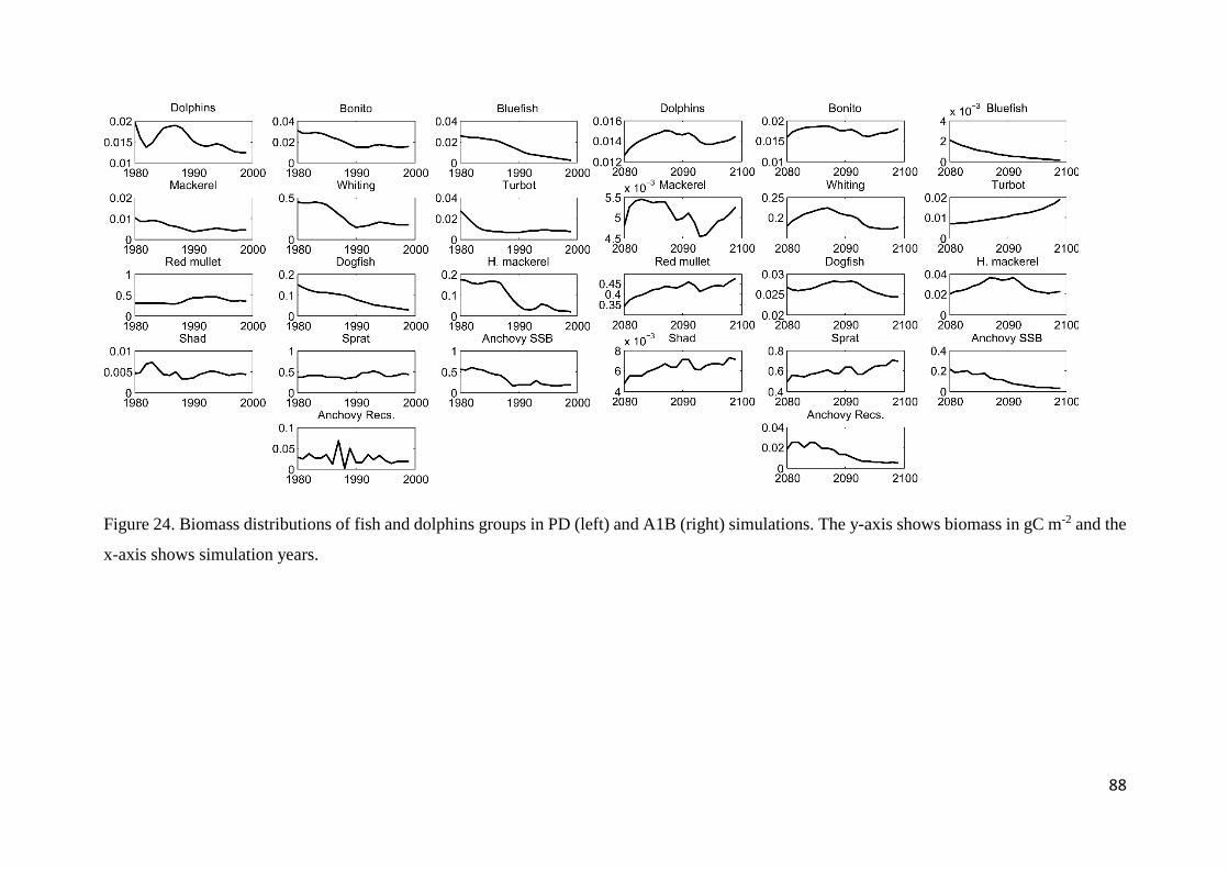
88
Figure 24. Biomass distributions of fish and dolphins groups in PD (left) and A1B (right) simulations. The y-axis shows biomass in gC m-2 and the
x-axis shows simulation years.

89
Figure 25. Fractional change predicted for fish and dolphin groups in A1B (2080-
2099) scenario relative to the PD (1980-1999) scenario.
5.3.4. Assessment of Indicators and Ratios
Considering the system’s throughput (TST), it decreased from a mean value of
436 gC m-2 y-1 in the early 1980s to a mean value of 353 gC m-2 y-1 in 1988 and
remained around this value after the anchovy-Mnemiopsis shift in the 1989-1990 until
the end of the PD scenario. The mean value of TST showed a marginal but significant
increase up to 371 gC m-2 y-1 with the onset of the A1B scenario due to the simulated
increase in the system’s primary productivity (Figure 26).
The system’s ascendency showed a significant shift in 1988 from 12.0% to a
mean value of 11.2% and afterwards, contrary to TST, no significant shift in the mean
value of this indicator was detected between PD and A1B scenarios (Figure 26). In
1988, the overhead (resilience) of the Black Sea ecosystem increased from a mean
value of 65.8% to 68.5% as a result of the decrease in the system’s ascendency. This
indicated that almost coinciding with the anchovy-Mnemiopsis shift, the Black Sea

90
ecosystem, afterwards, transitioned into a new state which could be characterised by
improved ecosystem conditions compared to the 1980s.
In the PD simulation, the relative primary production required to sustain
catches (%PPR) showed one significant shift in 1989 from an average value of 82% to
36% along with the collapse of the anchovy fishery. %PPR fluctuated around this lower
mean value throughout the rest of PD and entire A1B simulations (Figure 26). In
accordance with %PPR, the STARS algorithm identified one significant shift in the
annual mean value of the catches in the PD scenario. Catches showed a significant
decrease in 1990 from a mean value of 0.68 gC m-2 y-1 to 0.32 gC m-2 y-1 coinciding
with the collapse of anchovy stocks and the proliferation of Mnemiopsis in late 1980s.
The mean value of catch did not show any significant shift from its 1990s values and
remained at a lower level in the A1B scenario compared to 1980s simulated by the PD
scenario (Figure 26).
The STARS analysis detected a significant change in the mean value of the
system’s primary production, which was simulated by the BIMS-ECO model, in 1995
from 203 gC m-2 y-1 down to 165 gC m-2 y-1 (Figure 26) along with alleviating
eutrophic conditions with the onset of 1990s. With the start of the A1B simulation, in
accordance with the increased primary productivity simulated by the BIMS-ECO
model (Figure 19), the primary production showed a significant increase to a mean
value of 215 gC m-2 y-1 in 2083, which further increased up to a mean value of 241 gC
m-2 y-1 by the end of 2090s with the continuous increase of primary productivity in the
system (Figure 19).
The FiB index indicated a contraction in fisheries by means of quantity as a
consequence of decreasing fish stocks in the ecosystem (Figure 26). However, after its
shift in 1990 from a mean value of 0.013 to -0.006, the mean value of FiB index did
not show a significant change between PD and A1B scenarios. On the other hand, the
mTLc of the fleet changed significantly in the years 1990 and 2094 (Figure 26). The
first significant change in mTLc from a mean value of 3.12 to 3.06 in 1990 was a
consequence of the infamous anchovy-Mnemiopsis shift incident. The second shift
occurred by the end of the A1B scenario and mTLc decreased down to a value of 3.04.
The reason behind this decrease was the continuous decrease in the stocks of many
higher trophic level fish and dolphin groups in the A1B scenario along with the

91
increasing dominancy of particular lower trophic level demersal fish species, i.e. red
mullet, instead of its relatively higher trophic level demersal counterparts, i.e. whiting
and spiny dogfish. This resulted in the increasing dominancy of lower trophic level
fish species in the catches not only by means of the absence of higher trophic level
piscivorous fishes but also with the absence of higher trophic level demersal fish
assemblages. This compositional change in catch was also reflected by the changes in
Kempton’s Q indicator (Figure 26). The first shift in this indicator occurred in 1992
from a mean value of 0.76 to 1.024 after the anchovy-Mnemiopsis shift, which resulted
as an increase in the relative proportion of the organisms of and above trophic level III
in the ecosystem with the collapse of the anchovy stock. Kempton’s Q further
increased to 1.43 in 2080 with the changing conditions of the A1B scenario compared
to PD but this time by means of successful establishment of a high trophic level (TL >
III) jellyfish predator Beroe ovata. This latter increase was further intensified by the
continuous decrease of anchovy, the dominant fish in the ecosystem, stock in the Black
Sea by its continued intensive selective extraction during the A1B scenario, which, to
an extent, outcompeted the decrease in the higher tropic level fish species in the
ecosystem.
Considering the cycling properties of the ecosystem, the mean path length
travelled by a unit of energy increased from 4.96 to 6.23 in 1988 along with the
catastrophic disturbance of the system in 1989 by means of anchovy-Mnemiopsis shift
and further decreased down to 5.85 with the onset of the A1B scenario in 2080. This
showed that with the onset of 1990s along with alleviating eutrophic conditions, the
system transitioned into a more healthy state but with the onset of A1B scenario, the
increased primary productivity reverted this improvement backwards to some extent.
However, the FCI decreased from 3.05 to 1.93 in 1988 contrastingly (Figure 26). This
showed that the catastrophic shift of the 1989-1990 decreased the material cycling
along with Mnemiopsis’s overpopulation in the food web and this situation continued
with episodic blooms of Mnemiopsis in early 1990s and after the proliferation of Beroe
ovata in the ecosystem in 1997. The FCI showed a significant change in 2080 and
increased to 2.32 due to “relatively” decreasing dominancy of jellyfish and other
opportunistic organisms in the system moderated by the decrease in the system’s
primary productivity compared to the intensive eutrophic conditions of the 1980s. In
conjunction with these changes, the mean value of the proportion of flows to detritus,

92
after its first decrease in 1988 from 0.21 to 0.20, decreased further to 0.2 in 1997 until
its rise in 2091 to a mean value of 0.20 (Figure 26). This latest increase in the mean
value of the proportion of flows to detritus indicated that such a continuous increase
in the primary productivity of the system, i.e. nutrient enrichment, as simulated by the
BIMS-ECO model for the A1B scenario, had the possibility to revert the improved
conditions of the Black Sea food web obtained during the 1990s back to its undesired
state experienced during 1980s.
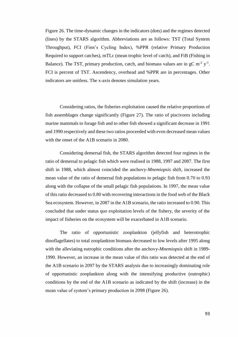
93
Figure 26. The time-dynamic changes in the indicators (dots) and the regimes detected
(lines) by the STARS algorithm. Abbreviations are as follows: TST (Total System
Throughput), FCI (Finn’s Cycling Index), %PPR (relative Primary Production
Required to support catches), mTLc (mean trophic level of catch), and FiB (Fishing in
Balance). The TST, primary production, catch, and biomass values are in gC m-2 y-1.
FCI is percent of TST. Ascendency, overhead and %PPR are in percentages. Other
indicators are unitless. The x-axis denotes simulation years.
Considering ratios, the fisheries exploitation caused the relative proportions of
fish assemblages change significantly (Figure 27). The ratio of piscivores including
marine mammals to forage fish and to other fish showed a significant decrease in 1991
and 1990 respectively and these two ratios proceeded with even decreased mean values
with the onset of the A1B scenario in 2080.
Considering demersal fish, the STARS algorithm detected four regimes in the
ratio of demersal to pelagic fish which were realised in 1988, 1997 and 2087. The first
shift in 1988, which almost coincided the anchovy-Mnemiopsis shift, increased the
mean value of the ratio of demersal fish populations to pelagic fish from 0.70 to 0.93
along with the collapse of the small pelagic fish populations. In 1997, the mean value
of this ratio decreased to 0.80 with recovering interactions in the food web of the Black
Sea ecosystem. However, in 2087 in the A1B scenario, the ratio increased to 0.90. This
concluded that under status quo exploitation levels of the fishery, the severity of the
impact of fisheries on the ecosystem will be exacerbated in A1B scenario.
The ratio of opportunistic zooplankton (jellyfish and heterotrophic
dinoflagellates) to total zooplankton biomass decreased to low levels after 1995 along
with the alleviating eutrophic conditions after the anchovy-Mnemiopsis shift in 1989-
1990. However, an increase in the mean value of this ratio was detected at the end of
the A1B scenario in 2097 by the STARS analysis due to increasingly dominating role
of opportunistic zooplankton along with the intensifying productive (eutrophic)
conditions by the end of the A1B scenario as indicated by the shift (increase) in the
mean value of system’s primary production in 2098 (Figure 26).

94
Figure 27. The time-dynamic changes in the ratios (dots) and the regimes detected
(lines) by the STARS algorithm. The x-axis denotes the simulation years.
5.3.5. Sensitivity of results to changes in fishing mortality
The simulated biomass values under three scenarios with three different fishing
mortality (F) rates, (F status quo, F with 50% increase and F with 50% decrease) were
shown in Figure 28. In the scenario with 50% less fishing mortality for all fish species,
the biomass of all fish species showed a significant increase with respect to the
scenario in which F values equalled to the status quo rates, and a 50% increase in
fishing mortality rates of the fish species resulted in a more moderate decrease in
simulated biomass values of the fish community within the Black Sea ecosystem.
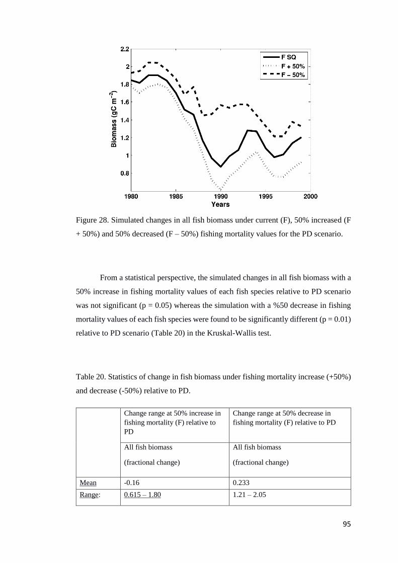
95
Figure 28. Simulated changes in all fish biomass under current (F), 50% increased (F
+ 50%) and 50% decreased (F – 50%) fishing mortality values for the PD scenario.
From a statistical perspective, the simulated changes in all fish biomass with a
50% increase in fishing mortality values of each fish species relative to PD scenario
was not significant (p = 0.05) whereas the simulation with a %50 decrease in fishing
mortality values of each fish species were found to be significantly different (p = 0.01)
relative to PD scenario (Table 20) in the Kruskal-Wallis test.
Table 20. Statistics of change in fish biomass under fishing mortality increase (+50%)
and decrease (-50%) relative to PD.
Change range at 50% increase in
fishing mortality (F) relative to
PD
Change range at 50% decrease in
fishing mortality (F) relative to PD
All fish biomass
(fractional change)
All fish biomass
(fractional change)
Mean -0.16 0.233
Range: 0.615 – 1.80 1.21 – 2.05

96
Percentile
25;
Percentile
75
-0.241, -0.065 0.085, 0.241
Test
Kruskal-
Wallis (p-
value)
0.0453 0.0094
The relative proportions of large fish by weight to the total fish biomass for the
three simulations with different fishing mortality levels were shown in Figure 29. In
all three scenarios, the changes in the large fish biomass were found to be significantly
different (p < 0.0001). This underlined the importance of fisheries management for
sustaining the relative proportions of fish stocks within a given ecosystem.
Figure 29. Large fish by weight in Present Day (PD) scenario for three different fishing
mortality regimes.

97
5.3.6. Experiments of Anchovy Stocks Collapse
The reasons behind the anchovy stock’s collapse were investigated under six
different scenario settings detailed in Table 19. All of the applied scenarios except
scenarios 3 and 4 simulated a decrease in the anchovy stock biomass in 1989-1990 and
a trailing decrease in the stock after 1993 (Figure 30). The trailing decrease was due
to the basin-wide decrease in primary production simulated by the biogeochemical
model, which was removed in constant primary productivity conditions in scenarios 2
and 4. The slight decrease in 1989-1990 observed in scenarios 3 and 4 was related to
the decrease in the forced zooplankton biomass values in that particular year.
Considering these, the decrease in 1989-1990 was related to a combination of the
impacts of fishing and over-proliferation of alien species Mnemiopsis, which in turn
caused a reduction in the zooplankton biomass in 1988-1989. Both of the scenarios
with Fmsy values applied on the anchovy stocks and with Fmsy values and an invariant
primary production equal to that in 1980 applied simulated the anchovy stocks collapse
in 1989-1990, whereas, scenario 2 did not experience a trailing decrease after 1995.
This showed that the trailing decrease was solely related to the simulated decrease in
the basin-wide primary production by the BIMS-ECO model. Scenario 3 with Fmsy
values applied and the invasion of alien ctenophores removed, the first collapse of the
anchovy stock in 1989-1990 vanished. Scenario 4, where Fmsy, an invariant primary
production equal to that in 1980 applied and the invasive ctenophores were removed
from the ecosystem, showed fluctuations, however, the simulated time series of the
anchovy biomass was stable to prevent any sort of sharp decrease considering the
criterion whether a simulated decrease/increase fell within the one standard deviation
distance of the simulated time series biomass data. Further, removal of Mnemiopsis
predation on anchovy eggs and larvae but keeping the Mnemiopsis’ predation pressure
on zooplankton in the system by means of forced zooplankton biomass values
(scenarios 3 and 4) still caused a slight decline in 1988-1989 in the anchovy stocks.
However, the opposite was not found to be true.

98
Figure 30. The simulated anchovy stock biomass progressions in PD; Scen. 1: Fmsy =
0.41; Scen. 2: Fmsy = 0.41 and constant primary production (~293.6 mgC m-2 day-1);
Scen. 3: Fmsy = 0.41 along with no Mnemiopsis and Beroe introduction; and Scen. 4:
Fmsy = 0.41, constant primary production (~293.6 mgC m-2 day-1) along with no
Mnemiopsis and Beroe introduction, Scen. 5: PD ecosystem conditions but with no
Mnemiopsis and Beroe introduction, and Scen 6: PD ecosystem conditions with
constant primary production (~293.6 mgC m-2 day-1).
In line with the simulated biomass predictions, the simulated catches showed
similar behaviour. The only scenarios in which such a collapse was not observed were
Scen. 3 and 4. Considering these, in a condition of invariant and constant primary
production equal to the initial conditions of the model and where no alien
invasions/introductions occurred, the maximum sustainable yield for the anchovy
stock was calculated to be able to reach ~300 000 kt with an exploitation rate (F/Z) of
0.14 (F = 0.41). However, in 2000s, the conditions were quite different than that of the
1990s. Considering the changes in primary production capacity (the decrease) of the
Black Sea ecosystem and the current stock progressions where invasive species were
present, sensitivity analysis of the Present Day model concluded that an MSY of ~200
kt with an exploitation rate of 0.11, which equalled Fmsy to 0.33, was possible (Figure

99
31) and will likely prevent catastrophic events like anchovy-Mnemiopsis shift in the
future under such circumstances where various environmental and trophic episodic
phenomena may occur.
Figure 31. The simulated anchovy stock catch progressions in PD; Scen. 1: Fmsy = 0.41;
Scen. 2: Fmsy = 0.41 and constant primary production (~293.6 mgC m-2 day-1); Scen.
3: Fmsy = 0.41 along with no Mnemiopsis and Beroe introduction; and Scen. 4: Fmsy =
0.41, constant primary production (~293.6 mgC m-2 day-1) along with no Mnemiopsis
and Beroe introduction, Scen. 5: PD ecosystem conditions but with no Mnemiopsis
and Beroe introduction, and Scen 6: PD ecosystem conditions with constant primary
production (~293.6 mgC m-2 day-1).
5.4. Discussions and conclusions
In this section, the reasons behind the collapse of small pelagic fish stocks, in
general, and anchovy-Mnemiopsis shift, in particular, occurred in 1989 were discussed
and this was followed by the explanations of relative changes between the PD and A1B
scenarios by means of the regime shifts in the synthetic indicators and ratios detected
100
by the STARS analysis. Finally, the management option for the fisheries on anchovy
stocks provided in the previous section was revisited considering the multi-species
interactions in the ecosystem.
The BIMS-ECO biogeochemical model simulated a decrease in the
zooplankton biomass with the appearance of the Mnemiopsis in the Black Sea
ecosystem. This was reflected as an increase in the phytoplankton biomass with the
onset of 1990s. This impact of decreased secondary production resources after/during
the anchovy-Mnemiopsis shift was observed in the decreasing biomass of forage fish
groups. According to Prodanov et al. (1997) and Daskalov (1998), heavy overfishing
could have led to this decline of the small pelagic fish stocks. Oguz et al. (2008b) also
underlined the competitive interference between Mnemiopsis and small pelagic fish.
As a contribution, I also related this decrease to changes in average primary
productivity of the 1990s. As indicated by the sensitivity experiments in section 5.3.5,
it could be concluded that the anchovy-Mnemiopsis shift occurred in 1989 was due to
the synergistic impacts of overfishing and resource competition with Mnemiopsis.
However, the impacts of both of these factors were mediated by the changes in the
primary productivity of the system. The predation of Mnemiopsis on anchovy eggs and
larvae was found to be negligible compared to trophic competition between anchovy
and Mnemiopsis. Finally, the experiments delineated that it could not be due to only
one single factor; i.e. overfishing (Daskalov, 2002; Gucu 2002; Llope, 2011) or trophic
competition and/or Mnemiopsis predation on anchovy eggs and larvae (Kideys, 2002).
The A1B simulation, along with the predicted basin-wide significant (p <
0.0001) increase in the primary production compared to the PD scenario due to
changes in circulation patterns, would have led an increase in the fish stocks, however,
under the assumption that the contemporary exploitation levels of fish species
continued, this inhibited the likely positive impact of such a productivity change.
The catch indicator showed significant changes between PD and A1B scenarios
according to the STARS analysis. This was a result of the continuation of the
unmanaged exploitation of the fish assemblages during the A1B scenario as shown by
the decreasing mTLc values throughout the simulation. This was also shown with the
three different regimes detected in the primary production indicator by the STARS
analysis between PD and A1B scenarios. The simulated increase in Kempton’s Q

101
index were not due to the recovery of the piscivorous fish stocks but rather due to the
simulated decrease in the forage fish biomass values for the A1B scenario, which in
turn, resulted in relatively increased proportions of the piscivorous fish both in the fish
community and the catches. Although a similar situation realised by the fishery
concerning lower trophic level fish species, i.e. small pelagic fish and most demersal
fish species, the decreases in the mTLc in A1B scenario indicated that the decreases
in the stocks of certain fish species in these assemblages were compensated by their
peers in their respective functional group of organisms (e.g. decrease in anchovy stocks
led to greater establishment of shad and sprat among the small pelagics; the decrease
in turbot and whiting led to greater establishment of red mullet among the demersals).
Considering the fractional change calculated for fish and marine mammal groups, all
of the populations except red mullet, shad and sprat were simulated to decrease (Figure
25).
Compared to the period after 1990s in the PD scenario, in A1B scenario the
proportion of flows to detritus was simulated to increase in 2091 along with the
increased primary productivity of the system. This underlined the fact that, in such
circumstances that will lead to increased productivity in the Black Sea, hence,
eutrophication, will likely reverse the rehabilitating structure of the ecosystem realised
by the onset of 1990s, leading to stress in the functioning of the food web and
deteriorate its integrity as it was the case during 1980s. Contrastingly, the FCI
increased with the onset of A1B simulation indicating better material cycling in the
food web. This indicated that the jellyfish populations will not have pronounced effects
in the ecosystem conditions predicted for the A1B scenario although enrichment of the
system was possible to some degree. However, towards the end of the A1B simulation,
the ratio of non-edible zooplankton to total zooplankton increased (Figure 27). This
indicated the tendency of the Black Sea ecosystem to return back to undesirable food
web conditions under predicted productivity increases. The decrease in the mean path
length indicator occurred with the onset of A1B scenario further supported this
interpretation.
Considering the multispecies interactions and an ecosystem-based approach to
the management of fish resources of the Black Sea, the calculated MSY value for
anchovy (see section 5.3.6) should be revisited. In order to obtain long-term consistent
yield from the anchovy stocks, a value of 200 kt at an exploitation rate of 0.11 was
102
found to be feasible. However, this exploitation intensity could only be succeeded in
a single-species, i.e. anchovy, dominant Black Sea ecosystem. With this exploitation
regime, recovery of the already depleted stocks of mackerel, bonito and bluefish would
not be possible. Further, the extinction of the Black Sea marine mammals was highly
expected by 2080 according to the simulation results of the A1B scenario (Figure 24,
Figure 27, and Figure 29). The sensitivity analyses carried out using the PD run put
forward that for the recovery of the Black Sea piscivorous fish and mammal stocks by
2080; strict management measures should be reinforced on the fishing fleet of the
Black Sea. First and foremost, only looking from the ecosystem perspective, the
fisheries for mackerel, bonito, and bluefish should end up in a complete halt. But this
perspective was found to be detrimental by means of socio-economic impacts on
fisheries. Therefore, a compromise should be made and in order to prevent such a
catastrophic effect, the fisheries of these species could be either subsided financially
or compensated by means of other value-added marketing of other profitable fish
products. However, only by minimising the fishing mortality for these groups proved
to be not sufficient for the recovery. Further considering the piscivorous fish and
mammals, the exploitation rate of forage fish groups should be rearranged sparingly
to ensure providing a consistent feeding stock for their recovery. Hence, the sensitivity
experiments indicated that anchovy catch should not exceed ~200 kt considering all
these implications. A value close to this estimation was also given by Oguz et al.
(2012).
In conclusion, the environmental conditions in the Black Sea simulated by the
A1B scenario will not be favourable from many aspects including the fishery as put
forward by means of indicators, ratios and fishing experiments. Further, continued
increase in system’s primary productivity by means of nutrient enrichment proved to
have a deteriorating impact on the functioning of the food web as shown by the analysis
of cycling indicators, i.e. FCI, proportional flows to detritus and mean path length.
This situation was found to bring about the possibility of reinstating the Black Sea
ecosystem back to its undesired conditions of 1980s. Under such an ecosystem state,
the regulation of fisheries as an activity could be focused on single species, i.e.
anchovy, so as to maximise the yield and the profit. However, in such circumstances,
fisheries of other target groups were simulated to disappear in the Black Sea and,
further, anchovy was predicted to be replaced by sprat under continuous exploitation.

103
Therefore, it was proposed to decrease the exploitation levels of the forage fish stocks
and completely halt the fisheries on piscivorous organisms for the sake of the Black
Sea ecosystem as well as its sustainability of economic goods and services in the long
term. The economic loss that would be created with such an action should also be
compensated by means of marketing strategies so as to alleviate the drawbacks by
introducing value-added capture production of other fisheries. This will increase the
prices of the capture fishes in the market marginally but compensate the
socioeconomic loss during the fisheries moratorium period for these target species.

104
6. CHAPTER: Thesis conclusions
6.1. Dynamics of the Black Sea Ecosystem
Considering the indicator-based analyses of ecological characteristics of the
Black Sea carried out in this thesis work, it was shown that the dynamics of the Black
Sea ecosystem during the second half of the 20th century were driven by two significant
factors; i) fisheries, and ii) eutrophication. The remaining processes of changes were
initiated by these two most significant factors as a series of a chain reaction.
First, during 1960s, the predatory species in the ecosystem were overexploited
by the fisheries as indicated by the decreasing mTLc and Kempton’s Q and increasing
PPR values. This was followed by the development of forage fish groups after the
release of predatory pressure on their stocks to dominate the system. Second, starting
with eutrophic conditions, the community size of small pelagic fish grew and
opportunistic species like jellyfish and Noctiluca became abundant. The resulting
ecosystem structure was dominated by forage fish in the higher trophic level and
opportunistic plankton species in the lower trophic level as shown by increasing
keystone values of these groups in 1980s. After the collapse of small pelagic fish
stocks in 1989, the eutrophic conditions started to alleviate and small pelagic fish
stocks started to recover. This new ecosystem structure of 1990s was characterised by
a medium stock level as shown by the biomass and catch indicators.
The sensitivity experiments using PD simulation showed that the most
significant factor for the anchovy stock collapse was fisheries and it was followed by
resource competition between small pelagic fish and opportunistic jellyfish species.
The outburst of Mnemiopsis contributed adversely to the ever-present resource
competition between small pelagic fish and jellyfish by outcompeting all the other
groups’ grazing on zooplankton with its high consumption to biomass ratio. The levels
of primary production were also influent on the progression of the anchovy stocks but
only due to the fact that it was one of the determining factors of available zooplankton
in the ecosystem. Further, considering the presence of voracious predators like
jellyfish, the deterministic factor of the resource availability to the forage fish species

105
was the grazing intensity on zooplankton by these opportunistic plankton. However,
none of these factors was found to be sufficient enough to cause such a catastrophic
anchovy-Mnemiopsis alone.
Future simulations of the Black Sea ecosystem (A1B) showed that, under
contemporary fishing exploitation levels, most significant fish species were likely to
experience significant decreases in their stocks. These species were found to be
anchovy, predatory species, and certain demersal fish species. In such circumstance,
due to released predation and resource competition pressures, species like sprat, shad
and red mullet will likely substitute these species in their respective environments and
develop their populations. Further, examining the indicators related to the energy flows
in the A1B scenario, it was shown that increased primary production in the Black Sea
bore the possibility to deteriorate the food web structure and functioning and cause
increasing dominancy of opportunistic organisms so as to reinstate undesirable
conditions of eutrophication across the food web. Under such situation, management
of fish stocks and their exploitation levels were found to be the most effective tool to
prevent catastrophic events in the ecosystem. However, sustainable management of
fish stocks could only be possible when considered together with their peers’ stock
dynamics rather than only evaluating the stock progressions of economically important
species in isolation from the ecosystem-wide impacts of anthropogenic and
climatologic stressors as well as the nonlinear interactions in the food web with other
lower and higher trophic level organisms.
6.2. The MSFD Perspective
Biological diversity (MSFD-D1, Table 21) of the Black Sea ecosystem had
experienced significant transformations since 1960s. The population biomasses of top
predatory species, i.e. dolphins, bluefish, bonito and mackerel, diminished to the extent
that their structuring role in the ecosystem almost vanished as put forward by the
keystoneness analysis (section 2.3.3). Further, the proportion of higher trophic level
organisms in the ecosystem decreased in time with the onset of 1970s due to continued
overexploitation of their stocks, which in turn, released the top-down control (section
106
2.3.3) exerted by these predatory species and this was followed by the resource
enrichment (section 2.3.5) in the Black Sea so that the development of lower trophic
level fish species, i.e. anchovy and sprat, and other gelatinous predators were promoted
(see Table 14 and Table 15). The decrease in the Kempton’s Q indicator starting from
1960s also reflected this shift in the dynamic simulations (sections 3.3.2 and 5.3.4).
All these changes brought the top predatory species almost to the brink of extinction
in the Black Sea (e.g. Atlantic mackerel) so that they could not self-sustain their
populations’ growth any longer. Future simulations put forward that these organisms
were likely to disappear completely from the Black Sea ecosystem if contemporary
fishing exploitation levels on these species prevailed in the future (section 5.3.3) and
the overexploitation of their food resources continued.
Concerning non-indigenous species (MSFD-D2, Table 21) in the Black Sea,
after 1988, Mnemiopsis became the most dominant zooplankton in the ecosystem until
mid-1990s. This was proven by the increasing keystoneness value of this organism
(section 2.3.3). Further, the feedbacks of this dominancy were quantified by the MTI
analysis (section 2.3), especially by the strong negative impact of Mnemiopsis against
small pelagic fish and trophic zooplankton. This was due to the changes in the energy
cycling through the food web, which was brought to the ecosystem along with the
increasing dominating role of gelatinous organisms in the 1970s and 1980s (section
2.3.4). The transfer efficiency of energy from primary producers to higher trophic level
groups was clogged by these gelatinous zooplankton and because they had no natural
predators in the ecosystem, the energy restrained by these organisms were “short-
circuited” back to detritus without contributing to the production of higher trophic
level organisms at and above trophic level III.
Commercial fish stocks (MSFD-D3, Table 21) were also negatively impacted
by all these changes. Their continuously high fishing mortalities caused a decline in
their stocks’ biomass along with the above mentioned transformations in the energy
cycling through the food web. Even the stocks of anchovy, the inexhaustible fish with
respect to fisheries in the ecosystem, continuously declined with the onset of 1980s
until its collapse in 1989 as simulated by the hindcast simulation of the time-dynamic
model (section 3.3.1) and to some extent, by the dynamic simulation of the coupled
model in section 5.3.1. This decrease was evident in the spawning stock biomass of

107
anchovy and also in the weakening recruitment power of the younger stages to the
adult stock (Figure 24).
The food web structure and functioning (MSFD-D4, Table 21) of the Black
Sea ecosystem had also experienced significant transformations. Concerning PPR, the
required primary production to sustain catches had increased continuously until the
collapse in 1989 (Figure 12). This structure was also supported by the decreasing ratio
of predatory fish to other fish and demersal fish to pelagic fish since the beginning of
the simulation period in 1960. Further, the trophic level decomposition of catches
(Table 14) and community biomass (Table 15) explicitly delineated the occurrence of
this shift with increasing ratio of lower trophic level fish and organisms in the catches
and in the community biomass respectively. Time-dynamic model results also
supported this hypothesis with the continuously decreasing large fish by weight
simulated from the beginning of 1960s (Figure 9). However, the most significant
change in the food web dynamics was the “short-circuiting” of flows back to detritus
by gelatinous organisms, hence, leaving the higher trophic level organisms up in the
food web deprived of the significant part of the system’s production which could have
been used for the growth of their populations. This short-circuiting was realized by
Aurelia and Noctiluca in the 1970s and 1980s until the outburst of Mnemiopsis.
Afterwards in the early 1990s, this short-circuiting was realised predominantly by
Mnemiopsis until the eutrophic conditions started to alleviate in the mid-1990s and
finally Beroe ovata arrived and settled in the ecosystem.
Eutrophication (MSFD-D5, Table 21) had also significant impact on the
ecosystem and could be regarded as the primary reason of the increased settlement of
the opportunistic, i.e. Noctiluca scintillans and/or r-selected (gelatinous species)
organisms in the ecosystem. This settlement led to the changes in the functioning of
the food web, hence, limiting the carrying capacity of the Black Sea ecosystem. The
negative impact of these changes were reflected in the decreasing overhead, i.e.
resilience, values of the ecosystem (Figure 8). In conjunction with other anthropogenic
(overfishing) and climatological (Oguz et al., 2008b) pressures, the Black Sea
ecosystem became famous for its rises and falls (Kideys, 2002) and was started to be
considered as a natural laboratory to investigate the impacts of synergistic effects of
concurrent alien introduction, overfishing, climatological changes and eutrophication
on the structure and functioning of a marine ecosystem.
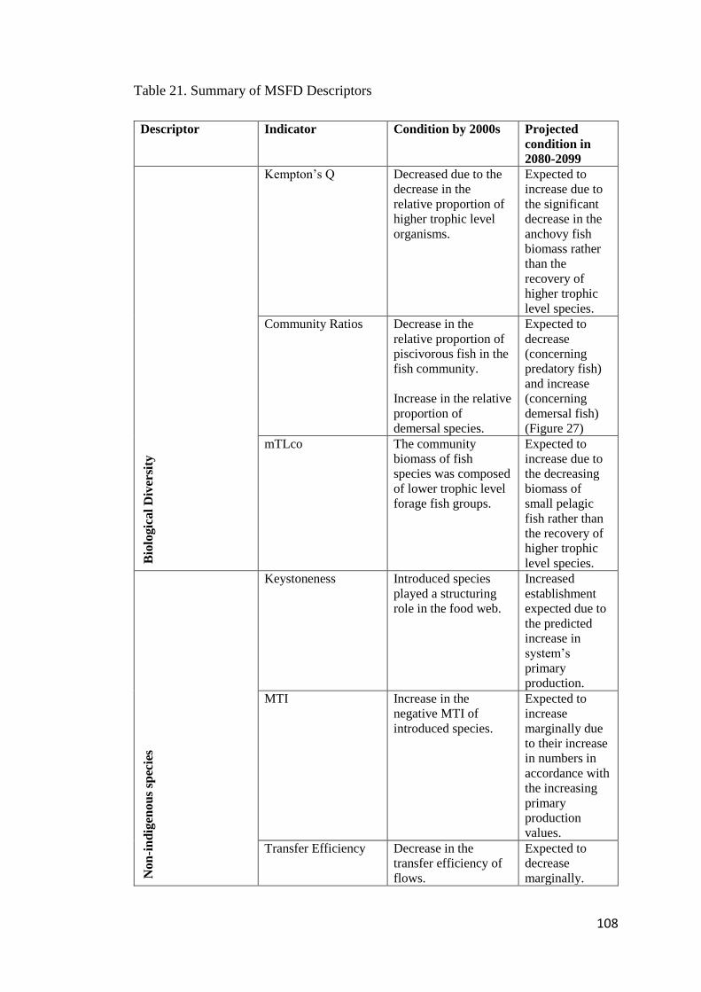
108
Table 21. Summary of MSFD Descriptors
Descriptor Indicator Condition by 2000s Projected
condition in
2080-2099 B
iolo
gic
al
Div
ersi
ty
Kempton’s Q Decreased due to the
decrease in the
relative proportion of
higher trophic level
organisms.
Expected to
increase due to
the significant
decrease in the
anchovy fish
biomass rather
than the
recovery of
higher trophic
level species.
Community Ratios Decrease in the
relative proportion of
piscivorous fish in the
fish community.
Increase in the relative
proportion of
demersal species.
Expected to
decrease
(concerning
predatory fish)
and increase
(concerning
demersal fish)
(Figure 27)
mTLco The community
biomass of fish
species was composed
of lower trophic level
forage fish groups.
Expected to
increase due to
the decreasing
biomass of
small pelagic
fish rather than
the recovery of
higher trophic
level species.
Non
-in
dig
eno
us
spec
ies
Keystoneness Introduced species
played a structuring
role in the food web.
Increased
establishment
expected due to
the predicted
increase in
system’s
primary
production.
MTI Increase in the
negative MTI of
introduced species.
Expected to
increase
marginally due
to their increase
in numbers in
accordance with
the increasing
primary
production
values.
Transfer Efficiency
Decrease in the
transfer efficiency of
flows.
Expected to
decrease
marginally.
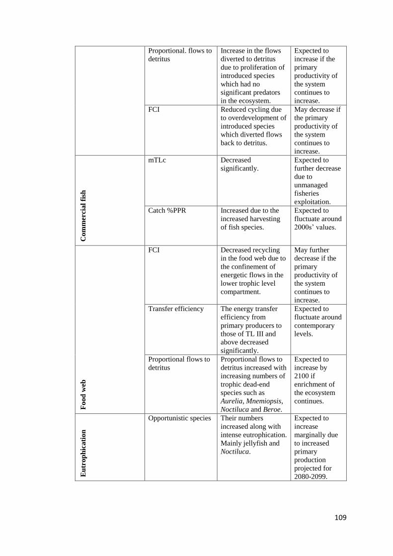
109
Proportional. flows to
detritus
Increase in the flows
diverted to detritus
due to proliferation of
introduced species
which had no
significant predators
in the ecosystem.
Expected to
increase if the
primary
productivity of
the system
continues to
increase.
FCI Reduced cycling due
to overdevelopment of
introduced species
which diverted flows
back to detritus.
May decrease if
the primary
productivity of
the system
continues to
increase.
Com
mer
cia
l fi
sh
mTLc Decreased
significantly.
Expected to
further decrease
due to
unmanaged
fisheries
exploitation.
Catch %PPR Increased due to the
increased harvesting
of fish species.
Expected to
fluctuate around
2000s’ values.
Fo
od
web
FCI Decreased recycling
in the food web due to
the confinement of
energetic flows in the
lower trophic level
compartment.
May further
decrease if the
primary
productivity of
the system
continues to
increase.
Transfer efficiency The energy transfer
efficiency from
primary producers to
those of TL III and
above decreased
significantly.
Expected to
fluctuate around
contemporary
levels.
Proportional flows to
detritus
Proportional flows to
detritus increased with
increasing numbers of
trophic dead-end
species such as
Aurelia, Mnemiopsis,
Noctiluca and Beroe.
Expected to
increase by
2100 if
enrichment of
the ecosystem
continues.
Eu
tro
ph
ica
tio
n
Opportunistic species Their numbers
increased along with
intense eutrophication.
Mainly jellyfish and
Noctiluca.
Expected to
increase
marginally due
to increased
primary
production
projected for
2080-2099.
110
References
Akaike, H., 1974. A new look at the statistical model identification. IEEE
Transactions on Automatic Control 19 (6), 716–723.
Barrett, R., Berry, M., Chan, T. F., Demmel, J., Donato, J., Dongarra, J.,
Eijkhout, V., Pozo, R., Romine, C., and van der Vorst, H, 1994. Templates for the
Solution of Linear Systems: Building Blocks for Iterative Methods, 2nd ed.
Philadelphia, PA: SIAM, 107 pp.
Beaugrand, G., 2004. The North Sea regime shift: Evidence, causes,
mechanisms and consequences. Progress in Oceanography, 60 (2–4), 245-262.
Berdnikov, S. V., Selyutin, V. V., Vasilchenko, V. V., Caddy, J. F., 1999.
Trophodynamic model of the Black and Azov Sea pelagic ecosystem: consequences
of the comb jelly, Mnemiopsis leidyi, invasion. Fisheries Research, 42, 261-289.
Bilio, M., and Niermann, U., 2004. Is the comb jelly really to blame for it all?
Mnemiopsis leidyi and the ecological concerns about the Caspian Sea. Marine Ecology
Progress Series 269, 173 – 183.
Birkun, A., 2008. The state of Cetacean populations. In: Oguz, T. (ed.), State
of the Environment of the Black Sea (2001 - 2006/7), Publications of the Commission
on the Protection of the Black Sea Against Pollution (BSC) 2008-3, Istanbul, Turkey,
pp. 365-396.
Blumberg, A. F., and Mellor, G. L., 1987. A description of a three dimensional
coastal ocean model. In: Heaps, N. (ed.), Three dimensional coastal ocean models,
A.G.U., Washington. pp. 1-16.
Cannaby, H., Fach, B. A., Akoglu, E., Salihoglu, B., 2012. Synthesis report for
Climate Simulations, Marine Ecosystem Evolution in a Changing Environment
(MEECE) Black Sea Regional Report D3.4, 51 pp.
Cardoso, A. C., Cochrane, S., Doerner, H., Ferreira, J. G., Galgani, F.,
Hagebro, C., Hanke, G., Hoepffner, N., Keizer, P. D., Law, R., Olenin, S., Piet, G. J.,

111
Rice, J., Rogers, S. I., Swartenbroux, F., Tasker, M., van de Bund, W., 2010. Scientific
Support to the European Commission on the Marine Strategy Framework Directive –
Management Group Report, Luxembourg: Office for Official Publications of the
European Communities, 57 pp.
Christensen V., and Cury P., 2005. Application of ecological indicators for
assessing health of marine ecosystems. In: Jorgensen, S. E., Costanza. R., Xu, F. L.,
(eds.) Handbook of ecological indicators for assessment of ecosystem health. Boca
Raton, FL, USA: CRC Press, pp. 193–212.
Christensen, V., 1995. Ecosystem maturity – towards quantification.
Ecological Modelling, 77, 3-32.
Christensen, V., and Caddy, J. F., 1993. Reflections on the pelagic food pelagic
food web structure in the Black Sea. In: Second Technical Consultation on Stock
Assessment in the Black Sea, Ankara, Turkey, 15-19 February. FAO Fisheries Report,
495, pp. 84-101.
Christensen, V., and Pauly, D. 1992. Ecopath II - a software for balancing
steady-state ecosystem models and calculating network characteristics. Ecological
Modelling, 61(3-4), 169-185.
Christensen, V., Walters, C. J., Pauly, D., 2005. Ecopath with Ecosim: A User's
Guide, Fisheries Centre, University of British Columbia, Vancouver, Canada, 154 pp.
Coll, M., Palomera, I., Tudela, S., Sarda, F., 2005. Trophic flows, ecosystem
structure and fishing impact in the South Catalan Sea, Northwestern Mediterranean. J.
Mar. Syst. 59, 63–96.
Coll, M., Santojanni, A., Palomares, I., Arneri, E., 2009. Food-web changes in
the Adriatic Sea over the last three decades. Mar Ecol Prog Ser, 381, 17–37.
Coll, M., Shannon, L. J., Moloney, C. L., Palomera, I., Tudela, S., 2006.
Comparing trophic flows and fishing impacts of a NW Mediterranean ecosystem with
coastal upwelling systems by means of standardized models and indicators, Ecological
Modelling, 198 (1–2), 53-70.

112
Costanza, R., 1992. Toward an operational definition of ecosystem health. In:
Costanza, R., Norton, B. G., Haskell, B. D. (eds.), Ecosystem Health: New Goals for
Environmental Management, Island Press, pp. 239–256.
Costanza, R., and Mageau, M., 1999. What is a healthy ecosystem? Aquatic
Ecology, 33, 105-115.
Cury, P., and Christensen, V., 2005. Quantitative ecosystem indicators for
fisheries management. ICES Journal of Marine Science, 62: 307-310.
Cury, P., Shannon, L., Roux, J., Daskalov, G., Jarre, A., Moloney, C., Pauly D.
2005. Trophodynamic indicators for an ecosystem approach to fisheries. ICES Journal
of Marine Science, 62, 430-442.
Daskalov G. M., 1998. Pêcheries et changement environmental à long-term en
mer Noire. PhD thesis. Centre d'océanologie de Marseille, Univ. Aix-Marseille II (in
French).
Daskalov, G. M., 2002. Overfishing drives a trophic cascade in the Black Sea.
Marine Ecology Progress Series, 225, 53-63.
Daskalov, G. M., 2003. Long-term changes in fish abundance and
environmental indices in the Black Sea. Marine Ecology Progress Series, 255, 259-
270.
Daskalov, G., Prodanov, K., Zengin, M., 2007. The Black Sea fisheries and
ecosystem change: discriminating between natural variability and human-related
effects. In: Proceedings of the Fourth World Fishery Congress, AFS Book, 1946 pp.
Diaz, S., and Cabido, M., 2001. Vive la différence: plant functional diversity
matters to ecosystem processes. TRENDS in Ecology & Evolution, Vol. 16, No.11.
Dow, D. D., O’Reilly, J. E., Green, J. R., 2006. Microzooplankton. In: Link, J.
S., Griswold, C. A., Methratta, E. T., Gunnard, J. (Eds.), 2006. Documentation for the
Energy Modelling and Analysis eXercise (EMAX). US Dep. Commer., Northeast
Fish. Sci. Cent. Ref. Doc. 06-15; 166 p.
Finn, J. T., 1976. Measures of ecosystem structure and function derived from

113
analysis of flows. J. Theor. Biol., 56, 363-380.
Froese, R. and Pauly, D. (eds.) 2011. FishBase. World Wide Web electronic
publication. www.fishbase.org, version (08/2011).
Fulton, E. A., 2010. Approaches to end-to-end ecosystem models. Journal of
Marine Systems, 81, 171–183.
Fulton, E. A., Anthony, A. D. M., Punt, A. E., 2005. Which ecological
indicators can robustly detect effects of fishing? ICES Journal of Marine Science, 62,
540-551.
Fulton, E.A., Link, J., Kaplan, I.C., Johnson, P., Savina-Rolland, M.,
Ainsworth, C., Horne, P., Gorton, R., Gamble, R.J., Smith, T., Smith D., 2011. Lessons
in modelling and management of marine ecosystems: The Atlantis experience. Fish
and Fisheries, 2:171-188.
Gaichas, S., Skaret, G., Falk-Petersen, J., Link, J. S., Overholtz, W., Megrey,
B. A., Gjøster, H., Stockhausen, W. T., Dommasnes, A., Friedland, K. D., Aydin, K.
Y., 2009. A comparison of community and trophic structure in five marine ecosystems
based on energy budgets and system metrics. Progress in Oceanography, 81, 47–62.
Grégoire, M., and Friedrich, J., 2004. Nitrogen budget of the northwestern
Black Sea shelf inferred from modelling studies and in situ benthic measurements Mar.
Ecol. Prog. Ser. 270, 15-39.
Gregoire, M., and Lacroix, G., 2003. Exchange processes and nitrogen cycling
on the shelf and continental slope of the Black Sea basin. Global Biogeochemical
Cycles, 17(2), 1073.
Gregoire, M., and Soetaert, K., 2010. Carbon, nitrogen, oxygen and sulphide
budgets in the Black Sea: A biogeochemical model of the whole water column
coupling the oxic and anoxic parts, 221(19), 2287-2301.
Gregoire, M., Raick, C., Soetaert, K., 2008. Numerical modelling of the central
Black Sea ecosystem functioning during the eutrophication phase. Progress in
Oceanography, 76, 286-333.
114
Gregoire, M., Soetaert, K., Nezlin, N., Kostianoy, A., 2004. Modelling the
nitrogen cycling and plankton productivity in the Black Sea using a three-dimensional
interdisciplinary model. Journal of Geophysical Research, 109, C05007.
Gucu, A. C., 2002. Can overfishing be responsible for the successful
establishment of Mnemiopsis leidyi in the Black Sea? Estuarine, Coastal and Shelf
Science, 54, 439-451.
Guénette, S., Heymans, S. J. J., Christensen, V., Trites, A. W., 2006.
Ecosystem models show combined effects of fishing, predation, competition, and
ocean productivity on Steller sea lions (Eumetopias jubatus) in Alaska. Canadian
Journal of Fisheries and Aquatic Sciences, 63, 2495-2517.
Haeckel, E., 1866. Generelle Morphologie der Organismen. Allgemeine
Grundzige der organischen Formen- Wissenschaft, mechanisch begriindet durch die
von Charles Darwin reformirte Descendenz-Theorie. 2 vols. Reimer, Berlin.
Haskell, B. D., Norton, B. G., Costanza, R., 1992. What is ecosystem health
and why should we worry about it? In: Costanza, R., Norton, B. G., Haskell, B. D.
(eds.), Ecosystem Health: New Goals for Environmental Management, Island Press,
pp. 3–19.
He, Y., Stanev, E. V., Yakushev, E., Staneva, J., 2012. Black Sea
biogeochemistry: Response to decadal atmospheric variability during 1960–2000
inferred from numerical modelling, Marine Environmental Research, 77, 90-102.
Kempton, R. A., and Taylor, L. R., 1976. Models and statistics for species
diversity. Nature, 262, pp. 818–820.
Kideys, A. E., Kovalev, A. V., Shulman, G., Gordina, A. and Bingel, F., 2000.
A review of zooplankton investigations of the Black Sea over the last decade. Journal
of Marine Systems, 24(2000), 355-371.
Kideys, E. A., 2002. Fall and rise of the Black Sea Ecosystem. Science 297,
1482-1483.
Kinzig, A. P., Ryan, P., Etienne, M., Allison, H., Elmqvist, T., Walker, B. H.,
115
2006. Resilience and regime shifts: assessing cascading effects. Ecology and Society
11(1), 20.
Konsulov, A. S., and Kamburska, L. T., 1998. Ecological determination of the
new Ctenophora Beroe ovata invasion in the Black Sea. Proceedings of the Institute
of Oceanology, Varna, 2, pp. 195–198.
Kovalev, A. V., and Piontkovski, S. A., 1998. Interannual changes in the
biomass of the Black Sea gelatinous zooplankton. Journal of Plankton Research, 20(7),
1377-1385.
Kovalev, A., Niermann, U., Melnikov, V., Belokopitov, V., Uysal, Z., Kideys,
A. E., Unsal, M., Altukhov, D., 1998. Long-term changes in the Black Sea
Zooplankton: The role of natural and anthropogenic factors. In: Ivanov L. I., and Oguz,
T. (eds.), Ecosystem Modelling as a Management Tool for the Black Sea. 2.
Environmental Security - Vol. 47, NATO Science Series, pp. 221-234.
Kruskal, W. H., and Wallis, W. A., 1952. Use of ranks in one-criterion variance
analysis. Journal of the American Statistical Association, 47 (260), 583–621.
Lalli, C. M., and Parsons, T. R., 1993. Biological oceanography: an
introduction. Pergamon Press, Oxford, 296 pp.
Lancelot, C., Stanevab, J., van Eeckhout, D., Beckers, J. M., Stanev, E., 2002.
Modelling the Danube-influenced North-western Continental Shelf of the Black Sea.
II: Ecosystem Response to Changes in Nutrient Delivery by the Danube River after its
Damming in 1972. Estuarine, Coastal and Shelf Science, 54(3), 473-499.
Langmead, O., McQuatters-Gollop, A., Mee, L. D. (Eds.). 2007. European
Lifestyles and Marine Ecosystems: Exploring challenges for managing Europe’s seas.
43pp. University of Plymouth Marine Institute, Plymouth, UK.
Lebedeva, L. P., and Shushkina, E. A., 1994. Modelling the effect of
Mnemiopsis on the Black Sea plankton community. Oceanology, Vol. 34(I), 72-80.
Levin, P. S., Fogarty, M. J., Murawski, S. A., Fluharty, D., 2009. Integrated
Ecosystem Assessments: Developing the Scientific Basis for Ecosystem-Based
116
Management of the Ocean. PLoS Biol 7(1): e1000014.
Libralato, S., Christensen, V., Pauly, D., 2006. A method for identifying
keystone species in food web models. Ecological Modelling, 195, 153-171.
Libralato, S., Solidoro, C., 2009. Bridging biogeochemical and food web
models for an End-to-End representation of marine ecosystem dynamics: The Venice
lagoon case study, Ecological Modelling 220: 2960–2971.
Lindeman, R. L., 1942. The trophodynamic aspect of ecology. Ecology, 23,
399-418.
Llope, M., Daskalov, G. M., Rouyer, T. A., Mihneva, V., Chan, K., Grishin,
A. N., Stenseth, N. C., 2011. Overfishing of top predators eroded the resilience of the
Black Sea system regardless of the climate and anthropogenic conditions. Global
Change Biology, 17, 1251–1265.
Lotka, A. J., 1920. Analytical Note on Certain Rhythmic Relations in Organic
Systems. Proc. Natl. Acad. Sci. 6, 410–415.
Marti, O., Braconnot, P., Bellier, J. R. B., Bony, S., Brockmann, P., Cadule, P.,
Caubel, A., Denvil, S., Dufresne, J. L., Fairhead, L., Filiberti, M. A., Foujols, M. A.,
Fichefet, T., Friedlingstein, P., Gosse, H., Grandpeix, J. Y., Hourdin, F., Krinner, G.,
Levy, C., Madec, G., Musat, I., Noblet, N. D., Polcher, J., Talandier, C., 2006. The
new IPSL climate system model: IPSL-CM4, Note du Pole de Modelisation, 26.
McQuatters-Gollop A., Mee, L. D., Raitsos, D. E., Shapiro, G. I., 2008.
Nonlinearities, regime shifts and recovery: the recent influence of climate on Black
Sea chlorophyll. Journal of Marine Systems, 74, 649–658.
Mee, L. D., 2006. Reviving dead zones. Scientific American 295, 54-61.
Möllmann, C., Diekmann, R., Muller-Karulis, B., Kornilovs, G., Plikshs, M.,
Axe, P., 2009. Reorganisation of a large marine ecosystem due to atmospheric and
anthropogenic pressure: a discontinuous regime shift in the Central Baltic Sea. Global
Change Biology, 15, 1377-1393.
Möllmann, C., Muller-Karulis, B., Kornilovs, G., and St. John, M. A., 2008.
117
Effects of climate and overfishing on zooplankton dynamics and ecosystem structure:
regime shifts, trophic cascade, and feedback loops in a simple ecosystem. ICES
Journal of Marine Science, 65, 302–310.
Mood, A. M., Graybill, F. A., Boes, D. C., 1974. Introduction to the Theory of
Statistics (3rd Edition). McGraw-Hill, 480 pp.
Nesterova, D., Moncheva, S., Mikaelyan, A., Vershinin, A., Akatov, V.,
Boicenco, L., Aktan, Y., Sahin, F., Gvarishvili, T., 2008. The state of phytoplankton.
In: Oguz, T. (ed.), State of the Environment of the Black Sea (2001 - 2006/7),
Publications of the Commission on the Protection of the Black Sea Against Pollution
(BSC) 2008-3, Istanbul, Turkey, pp 173-200.
O’Reilly, J. E., Dow, D. D., 2006. Phytoplankton and primary production. In:
Link, J. S., Griswold, C. A., Methratta, E. T., Gunnard, J. (Eds.), 2006. Documentation
for the Energy Modelling and Analysis eXercise (EMAX). US Dep. Commer.,
Northeast Fish. Sci. Cent. Ref. Doc. 06-15; 166 p.
Odum, E. P., 1969. The strategy of ecosystem development. Science, 104, 262-
270.
Odum, E. P., 1971. Fundamentals of Ecology. Saunders, Philadelphia, 574 pp.
Odum, E. P., 1985. Trends expected in stressed ecosystems, BioScience 35,
419– 422
Oguz, T., 2007. Nonlinear response of Black Sea pelagic fish stocks to over-
exploitation. Marine Ecology Progress Series, 345, 211-228.
Oguz, T., Akoglu, E., Salihoglu, B., 2012. Current state of overfishing and its
regional differences in the Black Sea. Ocean and Coastal Management, 58, 47-56.
Oguz, T., and Gilbert, D., 2007. Abrupt transitions of the top-down controlled
Black Sea pelagic ecosystem during 1960-2000: Evidence for regime-shifts under
strong fishery exploitation and nutrient enrichment modulated by climate-induced
variations. Deep-Sea Research, 54(I), 220-242.
Oguz, T., and Merico, A., 2006. Factors controlling the summer Emiliania
118
huxleyi bloom in the Black Sea: a modelling study. J. Marine Systems, 59, 173-188.
Oguz, T., and Salihoglu, B., 2000. Simulation of eddy-driven phytoplankton
production in the Black Sea. Geophysical Research Letters, 27(14), 2125-2128.
Oguz, T., and Velikova, V., 2010. Abrupt transition of the northwestern Black
Sea shelf ecosystem from a eutrophic to an alternative pristine state. Mar. Ecol. Prog.
Ser. 405, 231-242.
Oguz, T., Cokacar, T., Malanotte-Rizzoli, P., Ducklow, H. W., 2003. Climatic
warming and accompanying changes in the ecological regime of the Black Sea during
1990s. Global Biogeochem. Cycles, 17(3), 1088.
Oguz, T., Ducklow, H. W., Purcell, J. E., Malanotte-Rizzoli, P., 2001.
Modelling the response of top-down control exerted by gelatinous carnivores on the
Black Sea pelagic food-web. Journal of Geophysical Research, 106(C3), 4543-4564.
Oguz, T., Fach, B., Salihoglu, B., 2008a. Invasion dynamics of the alien
ctenophore Mnemiopsis leidyi and its impact on anchovy collapse in the Black Sea.
Journal of Plankton Research, 34(II), 1385-1397.
Oguz, T., Fach, B., Salihoglu, B., 2008b. A coupled plankton-anchovy
population dynamics model assessing nonlinear controls of anchovy and gelatinous
biomass in the Black Sea. Mar Ecol Prog Ser, 369, 229-256.
Orek, H., 2000. An application of mass balance Ecopath model to the trophic
structure in the Black Sea after anchovy collapse. M. S. in Marine Science, Middle
East Technical University, 119 pp.
Ozturk, B., Ozturk, A. A., Dede, A., 1999. Cetacean By-catch in the Western
Coast of the Turkish Black Sea in 1993-1997. In Evans, P. G. H., Cruz, J., Raga, J. A.,
(Eds.). Proc. 13th Annual Conf. European Cetacean Society, Valencia, Spain.
Pauly, D., Christensen, V., Dalsgaard, J., Froese, R., Torres, F., 1998. Fishing
down marine food webs. Science, 279, 860-863.
Pauly, D., Graham, W., Libralato, S., Morissette, L., Palomares Deng, M. L.,
2009. Jellyfish in ecosystems, online databases and ecosystem models. Hydrobiologia,

119
616, 67–85.
Petersen, C. G. J., 1903. What Is Overfishing?. Journal of the Marine
Biological Association, 6, 587-594.
Pianka, E. R., 1970. On r and K selection. American Naturalist 104(940), 592–
597.
Plaganyi, E. E., 2007. Models for an ecosystem approach to fisheries. FAO
Fisheries Technical Paper. No. 477. Rome, FAO, 108 pp.
Polovina, J. J., 1984. An overview of the ECOPATH model. Fishbyte, 2(2),
5-7.
Power, M. E., Tilman, D., Estes, J. A., Menge, B. A., Bond, W. J., Mills, L. S.,
Daily, G., Castilla, J. C., Lubchenco, J., Paine, R. T., 1996. Challenges in the quest for
keystones. Bioscience, 46(8), 609-620.
Press, W. H., Flannery, B. P., Teukolsky, S. A., and Vetterling, W. T., 1992.
"Runge-Kutta Method" and "Adaptive Step Size Control for Runge-Kutta." §16.1 and
16.2 in Numerical Recipes in FORTRAN: The Art of Scientific Computing, 2nd ed.
Cambridge, England, Cambridge University Press, pp. 704-716.
Prodanov, K., Mikhaylov, K., Daskalov, G., Maxim, K. and others, 1997.
Environmental management of fish resources in the Black Sea and their rational
exploitation. GFCM Stud. Rev., 68, 178 pp.
Rapport, D. J. 1992. Evolution of indicators of ecosystem health. In:
McKenzie, D. H., Hyatt, D. E., McDonald, V. J. (Eds.), Ecological Indicators.
Proceedings of the International Symposium on Ecological Indicators, Fort
Lauderdale, Florida, Elsevier Science, London, vol. 1, pp. 121-134., vol. 1:.
Rapport, D., Costanza, R., Epstein, P. R., Gaudet, C., Levins, R. 1998.
Ecosystem Health. Malden, MA, Blackwell Science.
Reid, P. C., Borges, M., Svendsen, E., 2001. A regime shift in the North Sea
circa 1988 linked to changes in the North Sea horse mackerel fishery. Fisheries
Research, 50, pp. 163–171.

120
Rodionov, S. N., 2004. A sequential algorithm for testing climate regime shifts.
Geophysical Research Letters, 31, L09204.
Rodionov, S. N., 2006. The use of prewhitening in climate regime shift
detection, Geophysical Research Letters, 31, L12707.
Rose, K. A., Allen, J. I., Artioli, Y., Barange, M., Blackford, J., Carlotti, F.,
Cropp, R., Daewel, U., Edwards, K., Flynn, K., Hill, S. L., HilleRisLambers, R., Huse,
G., Mackinson, S., Megrey, B., Moll, A., Rivkin, R., Salihoglu, B., Schrum, C.,
Shannon, L., Shin, Y. –J., Smith, S. L., Smith, C., Solidoro, C., St. John, M., Zhou,
M., 2010. End-To-End Models for the Analysis of Marine Ecosystems: Challenges,
Issues, and Next Steps, Marine and Coastal Fisheries: Dynamics, Management, and
Ecosystem Science, 2, 115-130.
Salihoglu, B., 2009. Effects of ENSO on the Cold Tongue and the Warm Pool
ecosystems in the equatorial Pacific Ocean: a modelling study. Journal of Marine
Systems, doi:10.1016/j.jmarsys.2008.12.004.
Salihoglu, B., Fach, B. A., Oguz, T., 2011. Control mechanisms on the
ctenophore Mnemiopsis leidyi population dynamics: A modelling study. Journal of
Marine Systems, doi:10.1016/j.jmarsys.2011.03.001.
Salihoglu, B., Neuer, S., Painting, S., Murtugudde, R., Hofmann, E. E., Steele,
J. H., Hood, R. R., Legendre, L., Lomas, M. W., Wiggert, J. D., Ito, S., Lachkar, Z.,
Hunt Jr., G. L., Drinkwater, K. F., and Sabine, C. L., 2013. Bridging marine ecosystem
and biogeochemistry research: Lessons and recommendations from comparative
studies, J. Mar. Syst., 109, 161–175.
Schaeffer, D. J., Henricks, E. E., Kerster, H. W., 1988. Ecosystem health: 1.
Measuring ecosystem health, Environ. Manage. 12, 445–455.
Shannon, L. J., Coll, M., Neira, S. 2009. Exploring the dynamics of ecological
indicators using food web models fitted to time series of abundance and catch data.
Ecological Indicators, 9, 1078–1095.
Shiganova, T. A., 1998. Invasion of the Black Sea by the ctenophore
Mnemiopsis leidyi and recent changes in pelagic community structure. Fish.

121
Oceanogr., 7(3/4), 305-310.
Shiganova, T. A., and Bulgakova, Y. V., 2000. Effects of gelatinous plankton
on Black Sea and Sea of Azov fish and their food resources. ICES Journal of Marine
Science, 57, 641-648.
Shiganova, T. A., Musaeva, E., Arashkevich, E., Kamburska, L., Stefanova,
K., Mihneva, M., Polishchuk, L., Timofte, F., Ustun, F., Oguz, T., 2008. The state of
zooplankton. In: Oguz, T. (ed.), State of the Environment of the Black Sea (2001 -
2006/7), Publications of the Commission on the Protection of the Black Sea Against
Pollution (BSC) 2008-3, Istanbul, Turkey, pp. 201-246.
Shin, Y. –J., Travers, M., Maury, O., 2010a. Coupling low and high trophic
levels models: Towards a pathways-orientated approach for end-to-end models.
Progress in Oceanography 84, 105–112.
Shin, Y.-J., Bundy, A., Shannon, L. J., Simier, M., Coll, M., Fulton, E. A.,
Link, J. S., Jouffre, D., Ojaveer, H., Mackinson, S., Heymans, J. J., and Raid, T.,
2010b. Can simple be useful and reliable? Using ecological indicators to represent and
compare the states of marine ecosystems. ICES Journal of Marine Science, 67, 717-
731.
Shin, Y.-J., Shannon L. J., Cury, P. M., 2004. Simulations of fishing effects on
the southern Benguela fish community using an individual based model: learning from
a comparison with ECOSIM. In: Ecosystem Approaches to Fisheries in the Southern
Benguela. Shannon, L. J., Cochrane, K. L. and S. C. Pillar (Eds.). African Journal of
marine Science 26: 95-114.
Shin, Y.-J., Shannon, L. J., Bundy, A., Coll, M., Aydin, K., Bez, N., Blanchard,
J. L., Borges, M. F., Diallo, I., Diaz, E., Heymans, J. J., Hill, L., Johannesen, E.,
Jouffre, D., Kifani, S., Labrosse, P., Link, J. S., Mackinson, S., Masski, H., Möllmann,
C., Neira, S., Ojaveer, H., Ould Mohammed Abdallahi, K., Perry, I., Thiao, D.,
Yemane, D., Cury, P. M., 2010c. Using indicators for evaluating, comparing and
communicating the ecological status of exploited marine ecosystems. Part 2: Setting
the scene. ICES Journal of Marine Science, 67, 692-716.
Shin, Y-J., Rochet, M-J., Jennings, S., Field, J. G., Gislason, H. 2005. Using

122
size-based indicators to evaluate the ecosystem effects of fishing. ICES Journal of
Marine Science, 62, 384–396.
Shlyakhov, V. A., and Daskalov, G. M., 2008. The state of marine living
resources. In: Oguz, T. (ed.), State of the Environment of the Black Sea (2001 -
2006/7), Publications of the Commission on the Protection of the Black Sea Against
Pollution (BSC) 2008-3, Istanbul, Turkey, pp. 321-364.
Staneva, J., Kourafalou, V., Tsiaras, K., 2010. Seasonal and Interannual
Variability of the North-Western Black Sea Ecosystem, TERR. ATMOS. OCEAN.
SCI., 21(1).
Steele, J. H., 1998. From carbon flux to regime shift. Fisheries Oceanography,
7(3/4), 176-181.
Steele, J. H., 2004. Regime shifts in the ocean: reconciling observations and
theory. Progress in Oceanography 60, 135–141.
Student, 1908. The probable error of a mean. Biometrika, Vol. 6(1), 1-25.
Tomczak, M. T., Müller-Karulis, B., Leili Jarv, Kotta, J., Martin, G., Minde,
A., Pollumae, A., Razinkovas, A., Strake, S., Bucas, M., Blenckner, T., 2009. Analysis
of trophic networks and carbon flows in South Eastern Baltic coastal ecosystems.
Progress in Oceanography, 81(1-4), 111-131.
Travers, M., Shin, Y. –J., Jennings, S., Cury, P., 2007. Towards end-to-end
models for investigating the effects of climate and fishing in marine ecosystems.
Progress in Oceanography, 75, 751–770.
Travers, M., Watermeyer, K., Shannon, L. J., Shin, Y. J., 2010. Changes in
food web structure under scenarios of overfishing in the southern Benguela:
Comparison of the Ecosim and OSMOSE modelling approaches. Journal of Marine
Systems, 79:101-111. DOI: 10.1016/j.jmarsys.2009.07.005.
Tsiaras, K., Kourafalou, V. H., Davidov, A., Staneva, J. 2008. A three-
dimensional coupled model of the western Black Sea plankton dynamics: Seasonal
variability and comparison to SeaWiFs data. J. Geophys. Res., 113, C07007.
123
Ulanowicz, R. E., 1986. Growth and development: ecosystem phenomenology.
Springer Verlag, New York, 203 pp.
Ulanowicz, R. E., 2004. Quantitative methods for ecological network analysis.
Computational Biology and Chemistry, 28(5-6), 321-339.
Ulanowicz, R. E., and Puccia, C. J., 1990. Mixed trophic impacts in
ecosystems. Coenoses, 5(1), 7-16.
Umani, S. F., Beran, A., Parloto, S., Virgilio, D., Zollet, T., de Olazabal, A.,
Lazzarini, B., Cabrini, M., 2004. Noctiluca scintillans Macartney in the Northern
Adriatic Sea: long-term dynamics, relationships with temperature and eutrophication,
and role in the food web. J. Plankton Res., 26(5), 545-561.
United Nations, 1992. Convention on Biological Diversity (CBD), Rio de
Janeiro, 28 pp.
Volterra, V., 1926. Variazioni e fluttuazioni del numero d’individui in specie
animali conviventi, Mem. Acad. Lincei, 2, 31–113.
Walters, C., Christensen, V., Pauly, D., 1997. Structuring dynamic models of
exploited ecosystems from trophic mass-balance assessments. Reviews in Fish
Biology and Fisheries, 7(2), 139-172.
Walters, C., Pauly, D., Christensen, V., and Kitchell, J. F. 2000. Representing
density dependent consequences of life history strategies in aquatic ecosystems:
EcoSim II. Ecosystems, 3(1):70-83.
Weslawski, J. M., Legeżyńska, J., 1998. Glaciers caused zooplankton
mortality? Journal of Plankton Research 20(7), 1233-1240.
Yunev, O. A., Carstensen, J., Moncheva, S., Khaliulin, A., Ærtebjerg, G.,
Nixon, S., 2007. Nutrient and phytoplankton trends on the western Black Sea shelf in
response to cultural eutrophication and climate changes. Estuarine, Coastal and Shelf
Science, 74, 63-76.
Yunev, O. A., Vedernikov, V. I., Basturk, O., Yilmaz, A., Kideys, A. E.,
Moncheva, S., Konovalov, S. K., 2002. Long-term variations of surface chlorophyll-a

124
and primary production in the open Black Sea. Mar Ecol Prog Ser, 230, 11–28.
Zaitsev, YU. P., 1992. Recent changes in the trophic structure of the Black Sea.
Fisheries Oceanography, 1(II), 180-189.
Zaitsev, YU. P., Mamaev, V., 1997. Biological Diversity in the Black Sea: A
Study of Change and Decline. United Nations Publications, New York, 208 pp.

125
CURRICULUM VITAE
PERSONAL INFORMATION
Surname, Name: Akoğlu, Ekin
Nationality: Turkish
Date and Place of Birth: 09 February 1982, Çanakkale
Marital Status: Married
Phone: +90 324 521 24 06
Fax: +90 324 521 23 27
Email: [email protected]
EDUCATION
Degree Institution Year of Graduation
PhD METU, Institute of Marine Sciences 2013
MS METU, Institute of Marine Sciences 2008
BS Istanbul University, Faculty of Fisheries 2004
High School İçel Anadolu High School, Mersin 2000
WORK EXPERIENCE
Year Place Enrolment
Feb, 2013 – Present METU, Inst. of Marine Sciences Project assistant
Dec, 2008 – Feb, 2013 METU, Inst. of Marine Sciences Research assistant
Oct, 2007 – July, 2008 METU, Inst. of Marine Sciences Project assistant
Oct, 2005 – Jan, 2007 METU, Inst. of Marine Sciences Project assistant
126
FOREIGN LANGUAGES
C2 English, A2 German, A1 Italian
PUBLICATIONS
1. Oguz, T., Akoglu, E. and Salihoglu, B., 2012. Current state of overfishing and its
regional differences in the Black Sea. Ocean and Coastal Management, 58(2012): 47
– 56.
2. Breen, P., Robinson, L. A., Rogers, S. I., Knights, A. M., Piet, G., Churilova, T.,
Margonski, P., Papadopoulou, N., Akoglu, E., Eriksson, A., Finenko, Z., Fleming-
Lehtinen, V., Galil, B., Goodsir, F., Goren, M., Kryvenko, O., Leppanen, J. M.,
Markantonatou, V., Moncheva, S., Oguz, T., Paltriguera, L., Stefanova, K., Timofte,
F., Thomsen, F., 2012. An environmental assessment of risk in achieving good
environmental status to support regional prioritisation of management in Europe.
Marine Policy, 36(5): 1033 – 1043.
3. Celebi B., Gucu A.C., Ok M., Sakinan S., Akoglu E., 2006. Hydrographic
indications to understand the absence of Posidonia oceanica in the Levant Sea (Eastern
Mediterranean). Biol. Mar. Medit., 13(4): 34 – 38.
HOBBIES
Playing the Guitar, Music Theory, Computer Technologies
Recommended