New Iterative Decoding Algorithms for
Low-Density Parity-Check (LDPC) Codes
by
Nastaran Mobini, B.Sc.
A thesis submitted to the
Faculty of Graduate and Postdoctoral Affairs
in partial fulfillment of the requirements for the degree of
Master of Applied Science in Electrical Engineering
Ottawa-Carleton Institute for Electrical and Computer Engineering
Department of Systems and Computer Engineering
Carleton University
Ottawa, Ontario
August, 2011
c©Copyright

The undersigned hereby recommends to the
Faculty of Graduate and Postdoctoral Affairs
acceptance of the thesis
New Iterative Decoding Algorithms for Low-Density
Parity-Check (LDPC) Codes
submitted by Nastaran Mobini, B.Sc.
in partial fulfillment of the requirements for the degree of
Master of Applied Science in Electrical Engineering
Professor Claude D’Amours, Examiner
Professor Ian Marsland, Examiner
Professor Amir Banihashemi, Thesis supervisor
Professor Thomas Kunz, Chair
iii

Abstract
Low-Density Parity-Check (LDPC) codes have gained lots of popularity due to their
capacity achieving/approaching property. This work studies the iterative decoding
also known as message-passing algorithms applied to LDPC codes. Belief propagation
(BP) algorithm and its approximations, most notably min-sum (MS), are popular
iterative decoding algorithms used for LDPC and turbo codes. The thesis is divided
in two parts. In the first part, a low-complexity binary message-passing algorithm
derived from the dynamic of analog decoders is presented and thoroughly studied.
In the second part, a modification for improving the performance of BP and MS
algorithms is proposed. It uses adaptive normalization of variable node messages.
v

Table of Contents
Abstract v
Table of Contents vi
List of Tables viii
List of Figures ix
Nomenclature xi
1 Introduction 1
1.1 Research Motivation and Contributions . . . . . . . . . . . . . . . . . 1
2 Channel Coding 4
2.1 Communication Systems . . . . . . . . . . . . . . . . . . . . . . . . . 4
2.2 Error Control Codes . . . . . . . . . . . . . . . . . . . . . . . . . . . 5
2.3 Block Codes . . . . . . . . . . . . . . . . . . . . . . . . . . . . . . . . 6
2.4 Low-Density Parity-Check Codes . . . . . . . . . . . . . . . . . . . . 8
2.5 Iterative Decoding . . . . . . . . . . . . . . . . . . . . . . . . . . . . 10
2.5.1 Hard-decision Algorithms . . . . . . . . . . . . . . . . . . . . 10
2.5.2 Soft-decision Algorithms . . . . . . . . . . . . . . . . . . . . . 11
3 Fixed Point Problem of Iterative Decoding 14
vi

3.1 Successive Substitution . . . . . . . . . . . . . . . . . . . . . . . . . . 15
3.2 Solving the First Order Differential Equation . . . . . . . . . . . . . . 18
4 Differential Binary Message Passing Decoding 22
4.1 Algorithm . . . . . . . . . . . . . . . . . . . . . . . . . . . . . . . . . 23
4.1.1 DD-BMP Algorithm . . . . . . . . . . . . . . . . . . . . . . . 24
4.1.2 Complexity . . . . . . . . . . . . . . . . . . . . . . . . . . . . 25
4.2 Simulation results . . . . . . . . . . . . . . . . . . . . . . . . . . . . . 27
5 Adaptive Belief Propagation Decoding of LDPC Codes 40
5.1 System Model and the Adaptive Control Technique . . . . . . . . . . 42
5.2 Simulation Results and Analysis . . . . . . . . . . . . . . . . . . . . . 44
6 Conclusions and Future Work 50
List of References 52
vii

List of Tables
4.1 Optimal values of q and 4∗ for different codes . . . . . . . . . . . . . 29
5.1 Breakdown of errors based on their type for the (1268,456) code, de-
coded by standard BP and adaptive BP, as a function of the maximum
number of iterations at different SNR values; “C”, “P” and “F” stand
for “Chaotic”, “Periodic” and “Fixed-pattern”, respectively. . . . . . 48
5.2 Breakdown of errors based on their type for the (504,252) code, de-
coded by standard BP and adaptive BP, as a function of the maximum
number of iterations at different SNR values; “C”, “P” and “F” stand
for “Chaotic”, “Periodic” and “Fixed-pattern”, respectively. . . . . . 48
viii

List of Figures
2.1 Elements of a communication system. . . . . . . . . . . . . . . . . . . 4
3.1 Illustration of the orbit of the function f(x) = λx(1−x) with different
values of λ. (a) illustrates an attractive fixed point, (b) repelling fixed
point, (c) periodic cycle and (d) chaos. . . . . . . . . . . . . . . . . . 16
3.2 BER curves of BP, MS, SR-MS for (1268,456) code. . . . . . . . . . . 19
3.3 Average number of iterations vs. BER for BP, MS, and SR-MS for
(1268,456) code. . . . . . . . . . . . . . . . . . . . . . . . . . . . . . . 20
3.4 BER curves of BP, MS, SR-MS for (504,252) code. . . . . . . . . . . 21
3.5 Average number of iterations vs. BER for BP, MS, and SR-MS for
(504,252) code. . . . . . . . . . . . . . . . . . . . . . . . . . . . . . . 21
4.1 BER vs. 4 for different values of q at SNR values 4 dB and 4.25 dB
for code (3000, 1000)(4,6). . . . . . . . . . . . . . . . . . . . . . . . . . 28
4.2 BER curves of BP, MS, DD-BMP, and GA for codes (3000, 1000)(4,6),
(6000, 2000)(4,6) and (12000, 4000)(4,6). . . . . . . . . . . . . . . . . . . 30
4.3 BER curves of BP, MS, DD-BMP, and GA for code (4000, 2000) with
different degree distributions. . . . . . . . . . . . . . . . . . . . . . . 31
4.4 BER curves of BP, MS, DD-BMP, and GA for code (1057, 813)(3,13). . 31
4.5 BER curves of BP, MS, IMWBF, DD-BMP, MDD-BMP and GA for
code (273, 191)(17,17). . . . . . . . . . . . . . . . . . . . . . . . . . . . 32
ix

4.6 BER curves of BP, MS, IMWBF, DD-BMP, MDD-BMP and GA for
code (1023, 781)(32,32). . . . . . . . . . . . . . . . . . . . . . . . . . . . 32
4.7 BER curves of BP, MS, DD-BMP, and GA for irregular code (1008, 504). 33
4.8 Average number of iterations vs. BER for BP, MS, DD-BMP and GA
for code (3000, 1000)(4,6), (6000, 2000)(4,6) and (12000, 4000)(4,6). . . . 35
4.9 Average number of iterations vs. BER for BP, MS, DD-BMP and GA
for code (4000, 2000) with different degree distributions. . . . . . . . . 35
4.10 Average number of iterations vs. BER for BP, MS, DD-BMP, and GA
for code (1057, 813)(3,13). . . . . . . . . . . . . . . . . . . . . . . . . . 36
4.11 Average number of iterations vs. BER for BP, MS, IMWBF, DD-BMP,
MDD-BMP and GA for code (273, 191)(17,17). . . . . . . . . . . . . . . 36
4.12 Average number of iterations vs. BER for BP, MS, IMWBF, DD-BMP,
MDD-BMP and GA for code (1023, 781)(32,32). . . . . . . . . . . . . . 37
4.13 Average number of iterations vs. BER for BP, MS, DD-BMP, and GA
for irregular code (1008, 504). . . . . . . . . . . . . . . . . . . . . . . 37
5.1 An example of Eq. (5.1). . . . . . . . . . . . . . . . . . . . . . . . . . 43
5.2 BER for a) (1268,456) and b) (504,252) LDPC codes decoded by stan-
dard BP, Normalized BP, and adaptive BP algorithms. . . . . . . . . 46
5.3 Average number of iteration versus BER for a) (1268,456) and b)
(504,252) LDPC codes decoded by standard BP, Normalized BP, and
adaptive BP algorithms. . . . . . . . . . . . . . . . . . . . . . . . . . 46
5.4 Iterative decoding trajectories for the (1268,456) LDPC code at
Eb/N0 = 2.5 dB: a) number of decision errors versus the iteration
number. b) E(i+1) vs. E(i) ; 1) fixed-pattern 2) periodic-pattern, and
3) random-like or chaotic. . . . . . . . . . . . . . . . . . . . . . . . . 47
x

Nomenclature
List of Acronyms
Acronym Explanation
AWGN Additive White Gaussian Noise
BCH Bose and Ray-Chaudhuri
BER Bit Error Rate
BF Bit Flipping
BP Belief Propagation
BPSK Binary Phase Shift Keying
DD-BMP Differential Decoding - Binary Message Passing
IMWBF Improved Modified Weighted Bit Flipping
LDPC Low-Density Parity-Check
LLR Log-Likelihood Ratio
LR Likelihood Ratio
xi

MBω Majority Based algorithms
MWBF Modified Weighted Bit Flipping
WER Word Error Rate
MS Min-Sum
SP Sum-Product
SS Successive Substitution
SR Successive Relaxation
WBF Weighted Bit Flipping
xii

List of Symbols
Symbol Explanation
0 all zero-vector or matrix depending on context
1 all-one vector
α normalization parameter
a a node in a Tanner graph
A coding alphabet
b a node in a Tanner graph
β normalization parameter
B`a,b memory content of the edge adjacent to node a and b in the `-th iteration
c a codeword (a row vector)
cj a check node
cth clipping threshold
C a binary linear code
dc degree of check node
dv degree of variable node
dmin minimum distance
dx/dy derivative of x with respect to y
xiii

E number of edges in a Tanner graph
E a posteriori average entropy
Eb energy of an information bit
f variable node operation
γ relaxation factor
G generator matrix
H parity-check matrix
Imax maximum number of iterations
k length of message
` iteration index
m a message word (a row vector)
m`a→b a message in LLR domain sent from node a to node b in the `-th iteration
ni zero-mean Gaussian noise
N block length of code equal to the number of variable nodes
N0 one-sided noise power spectral density
N (a) set of neighboring nodes of the node a
M number of check nodes
xiv

p0j(i) probability of j-th bit being “0” in the i-th iteration
p1j(i) probability of j-th bit being “1” in the i-th iteration
q number of quantized bits
Q quantization function
R code rate
σ2 noise variance
T transpose
vi a variable node
x a binary random variable
yi channel output corresponding to ci
zi hard decision value corresponding to i-th bit
xv

Chapter 1
Introduction
1.1 Research Motivation and Contributions
In the current century, the need for efficient and reliable digital data transmission and
storage systems has been significantly highlighted. Since 1962, when Gallager intro-
duced low-density parity-check (LDPC) codes along with various iterative decoding
algorithms [1], numerous encoding and decoding algorithms have been proposed and
standardized to fulfil the need. But it was not until 35 years later that the work
of MacKay and Neal [2, 3] brought LDPC codes back to light. Because of their very
good error correcting performance - close to the Shannon limit - they have been widely
studied and became part of various standards in the recent years [4–7].
Iterative decoding algorithms, also known as the message-passing algorithms are
used for decoding LDPC codes. An example is the belief propagation (BP) algorithm;
theoretically the most complex and the best decoding algorithm from the error rate
point of view that has been presented so far. There are lots of published papers with
emphasis on reducing the complexity of BP along with preserving its performance.
The min-sum (MS) algorithm [8] is a well-known approximation of BP that is much
easier to implement. The use of MS algorithm also eliminates the need for estimat-
ing the noise power in the communication channel which additionally reduces the
1

2
complexity of the decoder. A review of reduced complexity algorithms can be found
in [9]. In contrast with these works, several research groups have aimed to further
improve the performance of BP algorithm at the expense of more complexity [10–12].
In this thesis we propose one modification to the current algorithms and one new
low-complexity high-performance algorithm.
There is always a tradeoff between performance and complexity in the choice of
soft-decision and hard-decision algorithms. The hard-decision algorithms in compar-
ison to the soft-decision algorithms are considerably less complex but their perfor-
mance is not as good as soft-decision algorithms. In the first part of this thesis we
propose a new approach in which both the low complexity property of hard-decision
algorithms and the good performance property of soft-decision algorithms are pre-
served. We do this by adding memory with a limited number of bits to the Gallager
A algorithm which is a binary message-passing algorithm. The memory improves the
error rate of the proposed algorithm with only a moderate increase in complexity.
In second part we will introduce a modified versions of BP and MS algorithm
that only slightly changes the original iterative algorithm and can achieve better
performance in terms of bit error rate. The first proposed method can be applied to
both BP and MS algorithms and originates from the damping idea proposed in [11].
An adaptive control factor instead of a constant factor for damping is introduced.
Although this modification increases the complexity of the iterative decoder, there is
a noticeable improvement in bit error rate. The second proposed algorithm concerns
the analog implementation of the MS algorithm [13]. The Successive Relaxation
(SR) model was originally introduced for modeling the dynamics of analog iterative
decoders but it also can be used as an LDPC iterative decoder. The idea of using SR-
MS as an LDPC decoder has been studied in [14, 15]; the promising error correcting
property of this algorithm makes it an interesting research topic.
The rest of this thesis is organized as follow. In Chapter 2, a brief review of LDPC

3
codes and iterative decoding algorithms is given. Chapter 3 covers the conventional it-
erative algorithms. A new binary- message passing algorithm is introduced in Chapter
4. Adaptive MS based algorithms is given in Chapter 5. Finally, concluding remarks
and future work is addressed in Chapter 6.

Chapter 2
Channel Coding
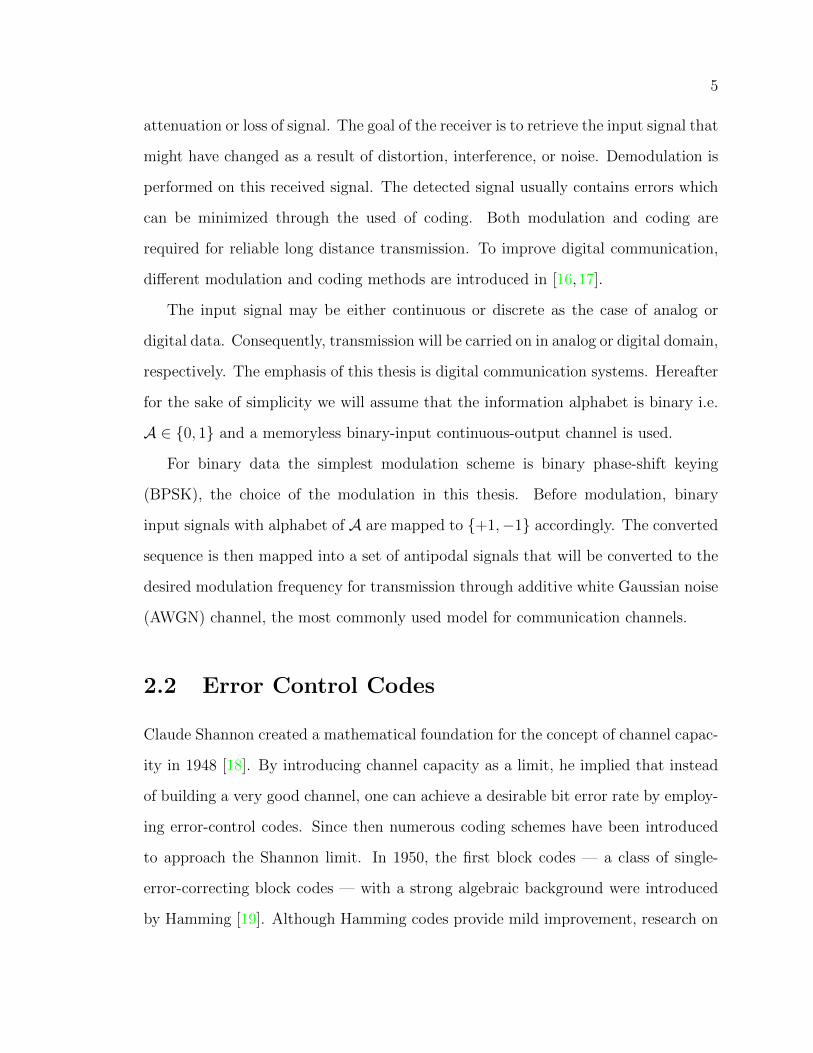
2.1 Communication Systems
A communication system provides us with a medium for transferring mutual infor-
mation through free space in the case of wireless communications or a pair of wires,
coaxial cable, or optical fibers in wired communications. A typical communication
system includes different elements such as the transmitter, transmission channel, and
receiver as shown in Fig. 2.1.
Figure 1. Elements of a communication system
TransmitterTransmission
ChannelReceiver
Input
Signal
Source Destination
Transmitted
Signal
Received
SignalOutput
Signal
Noise,interference, and
distortion
Figure 2.1: Elements of a communication system.
The input signal is processed in the transmitter considering the characteristic of
the transmission channel while the process almost always involves modulation and in
some cases coding. Then, transmission is conducted via the channel that can cause
4
5
attenuation or loss of signal. The goal of the receiver is to retrieve the input signal that
might have changed as a result of distortion, interference, or noise. Demodulation is
performed on this received signal. The detected signal usually contains errors which
can be minimized through the used of coding. Both modulation and coding are
required for reliable long distance transmission. To improve digital communication,
different modulation and coding methods are introduced in [16,17].
The input signal may be either continuous or discrete as the case of analog or
digital data. Consequently, transmission will be carried on in analog or digital domain,
respectively. The emphasis of this thesis is digital communication systems. Hereafter
for the sake of simplicity we will assume that the information alphabet is binary i.e.
A ∈ {0, 1} and a memoryless binary-input continuous-output channel is used.
For binary data the simplest modulation scheme is binary phase-shift keying
(BPSK), the choice of the modulation in this thesis. Before modulation, binary
input signals with alphabet of A are mapped to {+1,−1} accordingly. The converted
sequence is then mapped into a set of antipodal signals that will be converted to the
desired modulation frequency for transmission through additive white Gaussian noise
(AWGN) channel, the most commonly used model for communication channels.
2.2 Error Control Codes
Claude Shannon created a mathematical foundation for the concept of channel capac-
ity in 1948 [18]. By introducing channel capacity as a limit, he implied that instead
of building a very good channel, one can achieve a desirable bit error rate by employ-
ing error-control codes. Since then numerous coding schemes have been introduced
to approach the Shannon limit. In 1950, the first block codes — a class of single-
error-correcting block codes — with a strong algebraic background were introduced
by Hamming [19]. Although Hamming codes provide mild improvement, research on

6
the subject continued until the BCH codes [20,21] and Reed-Solomon codes [22] were
created a decade later. Along came the Convolutional codes [23] and their decoding
have been enhanced by the Viterbi algorithm [24]. But it wasn’t until the 1990s
that turbo codes were able to provide reliable communications with power efficiencies
close to the theoretical limit predicted by Shannon. A short time after that, another
type of codes known as Low-Density Parity-Check (LDPC) codes [25] with the same
capacity approaching property were rediscovered. On additive white Gaussian noise
(AWGN) channels, Turbo codes and LDPC codes both closely approach capacity by
the use of iterative decoding algorithms at the receiver.
During encoding, based on the input bits, redundant bits — to help the recovery
of the lost data — are added to the input sequence in order to form a codeword.
To maintain a good performance, the minimum distance between codewords should
be maximized. A binary code of size M has M = 2k binary codewords where k is
the number of information bits. The k-bits sequences are one by one converted to
codewords with block length of n, given n > k. Such a code is referred as an (n, k)
binary code. The amount of redundancy added to the input bits is measured by 1−R,
which R = k/n is called code rate.
2.3 Block Codes
A binary linear block code is defined by three parameters: the blocklength n, the
information length k, and the minimum distance d [26]. An (n, k) code is able to
correct t errors if its minimum distance satisfies the inequality 2t+ 1 ≤ d. The larger
the minimum distance, the better the code. Finding a good code is an important
issue in designing a communication system; the subject has been studied extensively
in the literature. In this thesis our focus is not on code design, but on the decoding.
7
A subspace of n-tuples over GF (2) is a binary linear code C, in which each n-
tuple that is called a codeword must satisfy the following conditions: the sum of
two codewords is another codeword. These codewords are used as the rows of a k
by n matrix G called the generator matrix of the code. The rows of G are linearly
independent, and the number of rows k shows the dimension of the code subspace
over GF (2). There are M = 2k binary codewords that can be found by
c = iG
where i is a k-tuple of information that is encoded to c the n-tuple codeword.
C as a subspace has an orthogonal complement C⊥ with dimension n− k, that is
also a subspace and can be used as a code. Therefore n − k linearly independent,
n-tuples as rows build an H matrix that is used in finding correct codewords of C.
Since a codeword of C is orthogonal to every row vector of H then
cHT = 0.
The matrix H is called the parity-check matrix of the code C. And consequently, the
matrix G is the parity-check matrix of the code C⊥.
Associated with the parity-check matrix there exists a bipartite graph with two
sets of nodes, known as a Tanner graph [27]. Considering an (n, k) code, the first set
containing n nodes with one by one relation to the codeword bits is called the variable
nodes set. The second set, check nodes set, represents the parity bits and consist of
n−k check nodes. These two sets are connected according to the parity-check matrix
of the code, an edge exists corresponding to each nonzero element in the parity-check
matrix.

8
2.4 Low-Density Parity-Check Codes
Low-density parity-check (LDPC) codes, sometimes called Gallager codes were first
proposed by Gallager in his thesis dissertation [25]. At that time they were considered
to be very complex due to the computational difficulties of the hardware of that time.
It was not until 30 years later that the work of Mackay [3, 28] brought them back
to light. Mackay showed that LDPC code ensembles can closely approach Shannon
capacity limit as block length increases [2], even closer than turbo codes [29]. Several
important factors such as: the capability of parallel decoding, less complexity per
iteration in comparison to that of turbo decoders, natural stopping criterion, error
floor at much lower BER than turbo codes, and the flexibility in the choice of rate and
codelength, have led them to appear in several standards, such as IEEE 802.16 [5],
IEEE 802.11 [6], IEEE 802.3 [4] and DBV-RS2 [7].
LDPC codes belong to the class of linear block codes and therefore are fully
described by their parity-check matrix. Their parity-check matrix is very sparse and
usually no two rows have more than one column in which they both have nonzero
elements (This means no cycle of length four in the Tanner graph). The number of
nonzero elements in each column or row is called the degree of that variable or check
node, respectively. If all the variable nodes have degree dv and all the check nodes
degree dc, the code will be a regular LDPC code otherwise an irregular one. The
design rate of a regular LDPC code is R = 1− dv/dc, where all the rows are linearly
independent; If not the actual rate will be higher than the design rate. Practical
LDPC codes have quite long block lengths while the variable and check node degrees
are around 3 or 4 in regular codes or as large as 10 to 15 in irregular codes, therefore
the density of nonzero elements in the parity-check matrix is very low — that is why
they are called low-density parity-check codes.
Each nonzero element in the parity-check matrix represents an edges in the Tanner

9
graph of the code connecting a variable node to a check node or vice versa. Neigh-
boring check nodes of a variable node are labeled byM(vi) = {cj : Hji = 1} and the
set of variable nodes connected to a check node is denoted by N (cj) = {vi : Hji = 1}.
Gallager showed that for constructing a good code, the row permutations should be
chosen at random out of n! possible choices. Good LDPC codes that have been found
are commonly computer generated and are very long, and because they don’t have
an algebraic structure their encoding is complicated. Encoding requires the generator
matrix which can be found based on H. To enhance the encoding, algebraic LDPC
codes based on finite geometries were derived [30]. They are constructed based on
well known finite geometries (FG) such as Euclidean and projective geometries over
finite fields. In [30], four classes of cyclic or quasi-cyclic FG LDPC codes known as
types I and II over these two geometries are described. Both types of FG LDPC
codes are regular, and they are the transpose of each other. Their encoding requires
simple linear feedback shift registers based on their generator (or characterization)
polynomials.
A binary J × n matrix HG whose rows and columns correspond to the lines and
points of a finite geometry G forms a FG LDPC code, if each row has dc and each
column dv 1s, while no two rows or columns have more than one 1 in common. G
is a finite geometry with n points and J lines. Each line consists of dc points and
two lines are either parallel (no intersection) or share only one point. Every point is
the intersect of dv lines and any two points are connected by one and only one line.
Extending a finite geometry LDPC codes is possible through splitting each column
or row of its parity-check matrix HG into multiple columns or rows. If properly done,
the extended code will perform very well [30].

10
2.5 Iterative Decoding
Iterative decoding algorithms based on their alphabet are generally divided into hard-
decision and soft-decision algorithms. The message alphabet can be as simple as
binary, e.g., A = {0, 1} or can consist of infinite uncountable number of symbols
such as the set of real numbers. If A is binary, the algorithm is referred to as
hard-decision; otherwise, it is called soft-decision. The computational complexity
of iterative algorithms usually increases with the alphabet size of messages.
2.5.1 Hard-decision Algorithms
In hard-decision algorithms, only binary values are used throughout the decoding
process. These algorithms are really important due to their simple implementation.
Their binary structure, binary memories and limited wiring, makes them remarkable
in hardware implementation especially in the situations where only hard-decision val-
ues are available at the receiver. Gallager’s algorithm A (GA) [1] is, for instance,
a hard-decision decoder in the set of Majority Based algorithms (MBω) [31] with
alphabet A = {−1, 1}. In MBω, a variable node passes its initial channel message
to any of its neighboring check nodes unless the majority of its extrinsic incoming
messages (ddv/2e + ω messages) contradict its initial message. In addition, the out-
going message of a check node is the product of its extrinsic incoming messages. The
MBω algorithms are studied in depth in [31], by the use of density evolution [32].
Another example of hard-decision algorithms is Bit Flipping algorithm (BF) [1]. In
this algorithm a flipping function is defined that counts the number of unsatisfied
syndrome bits (check nodes) in which each variable node participates. Each variable
node has a binary buffer to store a hard decision value; the content of this buffer will
be flipped if the corresponding output of the flipping function is more than a certain
threshold. Decoding continues until all check node equations are satisfied or until the
11
maximum number of iterations is reached.
2.5.2 Soft-decision Algorithms
In contrast to hard-decision algorithms, soft-decision decoding algorithms such as
belief propagation (BP) [3,27,32] and Weighted Bit Flipping algorithms (WBF) [30]
have a continuous alphabet. The BP algorithm is the most complex and the best
LDPC decoding algorithm from the error rate point of view. Much work has been
done to reduce the complexity of BP with the least effect on its performance. Min-sum
(MS) algorithm [8, 10, 33] is a well-known approximation of BP. A review of reduced
complexity algorithms can be found in [9]. The family of WBF algorithms shows
a good tradeoff between performance and complexity. Their performance is not as
good as that of BP but they are much simpler than BP and its approximations. In
other words, they provide good performance/complexity tradeoff. The family consists
of WBF algorithm, Modified Weighted Bit Flipping (MWBF) [34] and Improved
Modified Weighted Bit Flipping (IMWBF) [35]. The last two schemes are introduced
to improve the performance of the original WBF algorithm. Unlike BF, in these
algorithms only one bit is switched per iteration. The reliability of the received
inputs, which are the absolute values of the detector outputs, are employed in the
flipping function and only one hard-decision value associated to the variable node
that maximizes the flipping function is flipped.
Starting from WBF, different steps of each algorithm can be summarized in the
following lines. The check node process in WBF is finding the minimum reliability
among the reliability values of the variable nodes connected to that check node.
The flipping function is the weighted sum of the minimum reliability coming from
the check nodes connected to a variable node, in which the weighting factor is the
syndrome in {-1,1} domain. The check node process of MWBF is the same as WBF,
but the flipping function is modified by subtracting the weighted reliability value of

12
the corresponding variable node from the summation, where the weighting factor is
a constant. This modification improves the performance with a slight increase in
complexity of the algorithm. In IMWBF, the flipping function is different to some
extent. A check node sends different messages to the variable nodes connected to it, in
which the reliability of a variable node is excluded while calculating the message going
to that node. The flipping function is similar to that of MWBF except it uses the
extrinsic incoming messages. This increases the complexity and memory requirement
in comparison to the two other algorithms, but the performance is improved.
An iterative algorithm can be implemented in different domains e.g., probabil-
ity, likelihood ratio (LR) or log-likelihood ratio (LLR). In practice, LLR domain is
mostly used since message-passing algorithms are less complex and more robust in
this domain. BP algorithm in LLR domain can be summarized as follows. We use
the notations vi , i = 1, · · · , N , and cj , j = 1, · · · ,M , to denote the set of variable
nodes and the set of check nodes, respectively. The message sent from node a to node
b is denoted by ma→b.
1. Initialization
Variable node messages are initialized with received values yi from AWGN chan-
nel mvi→cj = 2σ2yi for i = 1, · · · , N and j = 1, · · · ,M .
2. Check node operation
mcj→vi = 2 tanh−1( ∏vk∈N (cj)\vi
tanh(mvk→cj
2
))(2.1)
3. Variable node operation
mvi→cj = mvi +∑
ck∈M(vi)\cj
mck→vi (2.2)

13
where mvi = 2σ2yi.
4. Hard decision
zvi = mvi +∑
ck∈M(vi)
mck→vi (2.3)
Vector z is quantized such that zi = 0 if zvi ≥ 0 otherwise zi = 1. If zHT = 0
decoding is completed, otherwise go to step 2. If a codeword cannot be found
within some specified maximum iterations a decoding failure is declared.
Computing the messages in check nodes is computationally complex. As previ-
ously mentioned, the most famous algorithm introduced for simplifying BP algorithm
is MS algorithm which approximates the check node operation as
mcj→vi =
( ∏vk∈N (cj)\vi
sign(mvk→cj)
)× min
vk∈N (cj)\vi|mvk→cj |. (2.4)
The operations performed in the variable nodes and for hard decision are those of
the BP algorithm.

Chapter 3
Fixed Point Problem of Iterative
Decoding
Decoding algorithms are employed to retrieve the original transmitted codeword over
a noisy channel. Since the closed-form solution of these algorithms is not obtainable,
iterative methods are used to approach an acceptable solution. One important ad-
vantage of iterative methods is their adaptivity, the system evolves as new messages
are made. Also, they might require fewer computations to get close to the final solu-
tion in comparison to the closed-form solution, which is especially attractive for some
applications where the need for speed is more critical than the need for precision.
Other than convergence speed, convergence itself is an essential issue in real-time sys-
tems. For some algorithms convergence can be proved by analytical methods while
for others only by computerize simulations. If done experimentally the convergence
can be determined for some degree of confidence.
In this chapter, an overview of current iterative methods used for decoding LDPC
codes is given. Then the new approach for solving the fixed-point problem of LDPC
decoding is presented.
14

15
3.1 Successive Substitution
Iterative decoding algorithms aim at solving a non-linear system of E equations with
E unknowns, where E = N × dv is the number of edges in the Tanner graph of
a regular LDPC code [36, 37]. Solutions to these equations are fixed-points which
might lead to a codeword or not. If a codeword is found the decoding is successful
otherwise an error or decoding failure is reported. An evolution equation can define
the discrete-time dynamical system of iterative decoding algorithm in the following
form
x(`+1) = f(x(`)) (3.1)
where f is the LDPC decoding function that maps the space RE into itself and x is
a vector of length E over the space RE whose initial value x(0) is arbitrary.
A fixed point x is found when application of f doesn’t change the value, i.e.
x = f(x). Finding fixed-points by putting Eq. (3.1) into the recursion is a classical
approach and is called the successive substitution (SS) method [38]. Most of the
conventional iterative decoding algorithms use this approach, e.g. the BP and MS
algorithm.
Combining two equations of variable nodes and check nodes of an LDPC decoding
algorithm leads to a fixed point problem of
x(`+1) = f(x(`),y(0)) (3.2)
where y(0) is the received vector with length N . The set of points x(`), ` = 0, 1, 2, . . .
is called the orbit of the point x under the transformation f .
Fig. 3.1 shows different behavior of the example function f(x) = λx(1 − x) for
various λ values. We can see (a) attractive fixed point (b) repelling fixed point (c)
periodic cycle and (d) chaos.

16
0 0.5 10
0.2
0.4
0.6
0.8
1(a) λ=2.5
0 0.5 10
0.2
0.4
0.6
0.8
1(c) λ=3.2
0 0.5 10
0.2
0.4
0.6
0.8
1(d) λ=3.9
0 1 2 3 4
0
1
2
3
4
5(b) λ=−1
Figure 3.1: Illustration of the orbit of the function f(x) = λx(1− x) with differentvalues of λ. (a) illustrates an attractive fixed point, (b) repelling fixed point,(c) periodic cycle and (d) chaos.

17
In general, iterative algorithms can demonstrate any of the above behaviors known
to occur in a nonlinear dynamical systems. Based on the initial vector, the behavior
of a general dynamical system lies within following classes:
• Regular attractors: fixed-point, periodic orbits, and limit cycles;
• Irregular attractors: chaotic and strange attractors.
But only one of them, the stable unequivocal fixed-point, is desirable in which
estimated LLRs found through iterations are close to negative or positive infinity.
When the decoder converges to an indecisive fixed-point that leads to a codeword
— estimated LLRs are close to zero — an undetected error is observed which is a
serious problem because in real systems this type of error will remain unnoticed and
potentially can cause trouble. If the orbit of iterative decoder matches any class other
than unequivocal fixed-point usually the chance of observing a codeword approaches
zero [36]. In the case of periodic orbits and limit cycles there is a k in which x` = x`+k
and x never approaches the desired solution similar to chaotic and strange attractors
but in the two last ones the behavior of x is unpredictable. Different methods are
introduced to help the convergence of iterative decoders by pulling it out of periodic
orbits [39, 40] or chaos [36].
Numerous numerical methods have been introduced to improve the convergence
property of iterative decoders especially turbo decoders [41]. Although for turbo de-
coders the SS method has the best performance, for LDPC decoders other approaches
such as Gauss-Seidel [33, 42–44] and Successive Relaxation [13] have shown promis-
ing improvement in performance in comparison to that of SS based approaches. In
Section 3.2 these methods are reviewed and a scheme for improving Successive Re-
laxation method applied to MS algorithm is proposed. But before that we would like
to introduce a new modification for conventional implementation of BP algorithm.
This modification helps the iterative decoder to converge which means a better error
correcting probability.

18
3.2 Solving the First Order Differential Equation
The first order differential equation
x(t) = f(x(t))− x(t), t ≥ 0 (3.3)
is interpreted as an analog or continues time representation of the iterative decoder.
In [13,37,45,46] it is pointed out that Eq. (3.3) expresses the dynamic of continuous-
time analog iterative decoding.
The under relaxed version of Eq. (3.1) with a relaxation parameter γ ∈ (0, 1] can
be used to solve the Eq. (3.3). The below method is called Successive Relaxation
(SR).
x(`+1) = (1− γ)x(`) + γf(x(`)). (3.4)
The successive relaxation method employs the current value of x to estimate the
future value. In SS method the value found by f(x(`)) is considered as the new
estimate of the fixed-point in the ` + 1th iteration. But in SR method both f(x(`))
and x(`) with a certain proportion are used to create the new estimate. For example,
SR implementation of MS algorithm is possible by simply modifying the variable node
operation and the rest of iterative algorithm is untouched. In MS algorithm x is the
vector of variable node messages mv→c going to check nodes. Updating mv→c is done
by doing the original check node and variable node operations represented by f and
then involving the current value in the following form
m`+1v→c = (1− λ)m`
v→c + λf(m`v→c). (3.5)
Simulation results have proved the superior performance of SR implementation
of MS algorithm over SS implementation [14]. By a slight change in variable node

19
1 1.5 2 2.510
−7
10−6
10−5
10−4
10−3
10−2
10−1
Eb/N
0 (dB)
BE
R
SS−BPSS−MSSR−MS
Figure 3.2: BER curves of BP, MS, SR-MS for (1268,456) code.
operation of MS algorithm which is particularly of interest because of its low com-
plexity the performance has shown a considerable improvement. Let us call the SR
implementation of MS as SR-MS. Two codes (1268,456) and (504,252) taken from [47]
and [48] respectively, have been tested and the simulation results are given in Fig. 3.2
to 3.5. It is assumed that BPSK modulated codewords are transmitted through an
AWGN channel and are decoded with three algorithms while the maximum number
of iterations is 200 and enough codewords are simulated to generate 100 codeword
errors. The performance curves for the BP algorithms are given for reference. The
bit error rate curves generated by SR-MS are very close to those of BP algorithm and
even better in higher SNRs. The gaps between MS and SR-MS for code (1268,456)
and (504,252) are 0.4 dB and 0.3 dB respectively, even larger than the gap between
BP and MS. Even in terms of the average number of iterations SR-MS is close to
other algorithms and they all approach the same value for higher SNRs. Comparing
the complexity of BP algorithm with that of SR-MS algorithm, makes SR-MS a very
good substitute for BP in fast and real-time applications. The only drawback is the

20
10−7
10−6
10−5
10−4
10−3
10−2
10−1
5
10
15
20
25
30
35
40
BER
Ave
rage
Num
ber
of It
erat
ions
SS−BPSS−MSSR−MS
Figure 3.3: Average number of iterations vs. BER for BP, MS, and SR-MS for(1268,456) code.
need for extra memory elements to store the previous variable node messages. Each
edge requires its own memory that makes the total of E = N × dv memories.
Inspired by the idea of memories in the variable nodes we have designed a new
binary message passing algorithm for decoding LDPC codes [49, 50]. The algorithm
incorporates soft information by storing the quantized received values and differen-
tially updating them in each iteration based on the extrinsic binary messages from
the check nodes. While the binary message-passing is particularly attractive for its
low complexity and simple implementation (translating to lower area and power con-
sumption in VLSI chips), the incorporation of soft information provides more coding
gain and improves the performance. The details of this new algorithm which is a
binary implementation of SR-MS algorithm can be found in the following Chapter.

21
1.5 2 2.5 3 3.510
−7
10−6
10−5
10−4
10−3
10−2
10−1
Eb/N
0 (dB)
BE
R
SS−BPSS−MSSR−MS
Figure 3.4: BER curves of BP, MS, SR-MS for (504,252) code.
10−7
10−6
10−5
10−4
10−3
10−2
10−1
0
5
10
15
20
25
30
35
BER
Ave
rage
Num
ber
of It
erat
ions
SS−BPSS−MSSR−MS
Figure 3.5: Average number of iterations vs. BER for BP, MS, and SR-MS for(504,252) code.

Chapter 4
Differential Binary Message Passing
Decoding
In this chapter, we propose a binary message-passing algorithm for decoding low-
density parity-check (LDPC) codes. The algorithm substantially improves the per-
formance of purely hard-decision iterative algorithms with a small increase in the
memory requirements and the computational complexity. We associate a reliability
value to each nonzero element of the code’s parity-check matrix, and differentially
modify this value in each iteration based on the sum of the extrinsic binary messages
from the check nodes. For the tested random and finite-geometry LDPC codes, the
proposed algorithm can achieve performance as close as 1.3 dB and 0.7 dB to that of
belief propagation (BP) at the error rates of interest, respectively. This is while, un-
like BP, the algorithm does not require the estimation of channel signal to noise ratio.
Low memory and computational requirements and binary message-passing make the
proposed algorithm attractive for high-speed low-power applications.
22

23
4.1 Algorithm
We consider the application of a binary LDPC code C over a binary-input AWGN
channel. Coded bits 0 and 1 are mapped to channel input symbols +1 and −1,
respectively. The channel is memoryless and at the channel output, the received
value yi corresponding to the transmitted symbol xi is given by yi = xi+ni, where ni
is a zero-mean Gaussian noise with variance σ2 independent of xi. Assuming that the
AWGN has a power spectral density N0/2, we have σ2 = 1/(2REb/N0), where Eb and
R denote the energy per information bit and the code rate, respectively. Suppose that
C is a regular (n, k)(dv ,dc) code with length n described by an (n− k)×n parity check
matrix H = [Hij], where dv and dc represent the number of ones in each column and
each row of H, respectively. They also represent the degrees of variable and check
nodes in the Tanner graph of C, respectively.
To implement the algorithm, we consider the received values to be clipped sym-
metrically at a threshold cth, and then uniformly quantized in the range [−cth , cth].
We use the notation Q(yi) to denote the quantized value of yi. There are 2q−1 quan-
tization intervals, symmetric with respect to the origin. Each quantization interval
has a length ∆ = 2cth2q−1 and is represented by q quantization bits. Integer numbers
−(2q−1 − 1), · · · , 2q−1 − 1 are assigned to the intervals. We associate a q-bit memory
to each edge in the graph, and initialize it with the quantized received value of the
adjacent variable node. The content of this memory is differentially updated in each
iteration by being incremented or decremented according to the sum of the extrinsic
binary messages of the check nodes. The operations in the check nodes are XOR and
the binary message passed from a variable node to a check node is the sign of the
memory associated with the edge connecting the two nodes. Decisions are made on
the values of variable nodes in each iteration according to the majority of the signs of
the adjacent edge-memories and the sign of the initial received value. The decoding

24
is stopped if the decisions satisfy the parity-check equations or if a maximum number
of iterations Imax is reached.
We use the notations vi , i = 1, · · · , N , and cj , j = 1, · · · ,M , to denote the set
of variable nodes and the set of check nodes, respectively. The message sent from
node a to node b at iteration ` is denoted by m`a→b. All the messages passed between
variable and check nodes are binary with alphabet A = {+1,−1}. Notation B`vi,cj
is
used for the memory content of the edge adjacent to vi and cj at iteration `. The
algorithm is then described by the following steps:
4.1.1 DD-BMP Algorithm
1. Initialization, ` = 0
z(0)i = (1− sgnr(yi))/2, i = 1, · · · , N where sgnr(x) = 1, for x > 0, and = -1
for x < 0. (For x = 0, sgnr(x) takes +1 or -1 randomly with equal probability.)
Let z (0) = (z(0)1 , · · · , z(0)N ). If z (0)HT = 0, the decoding is stopped and the
transmitted codeword is estimated by z(0). Otherwise, the memory contents
are initiated by B(0)vi,cj = Q(yi), i = 1, · · · , N, j = 1, · · · ,M , for i and j values
that satisfy Hij = 1. The initial messages from variable nodes to check nodes
are m(0)vi→cj = sgnr(B
(0)vi,cj). The algorithm is then continued at step 2.
2. Check Operation, ` ≥ 1
m(`)cj→vi =
∏vk∈N (cj)\vi
m(`−1)vk→cj (4.1)
where N (b) denotes the neighboring nodes of node b, and N (b)\a denotes N (b)
excluding a.

25
3. Variable Operation and Memory Update, ` ≥ 1
B(`)vi,cj
= B(`−1)vi,cj
+∑
ck∈N (vi)\cj
m(`)ck→vi (4.2)
m(`)vi→cj = sgnr(B
(`)vi,cj
) (4.3)
4. Hard-Decision, ` ≥ 1
D(`)i =
∑cj∈N (vi)
sgn(B(`)vi,cj
) + sgn(yi), (4.4)
z(`)i =
1− sgn(D(`)i )
2, i = 1, · · · , N, if D
(`)i 6= 0 (4.5)
where sgn(x) = 1, for x > 0; = -1 for x < 0; and = 0, for x = 0. For
D(`)i = 0, z
(`)i = z
(`−1)i . The algorithm is stopped if z (`)textbfHT = 0 , or if
` = Imax. (In the former case, z (`) is used as an estimate for the transmitted
codeword, while in the latter case a decoding failure is declared.) Otherwise,
` = `+ 1, and the algorithm is continued from Step 2.
4.1.2 Complexity
To evaluate the complexity of the proposed algorithm, we first consider the number
of operations per iteration. In the check nodes, to implement Eq. (4.1) directly, we
need to perform E × (dc − 2) binary XOR operations or binary multiplications, for
the {0, 1} alphabet or the {−1, 1} alphabet, respectively, where E = N × dv is the
number of edges in the graph. This can be reduced to less than 2E if we first compute
Eq. (4.1) over all N (cj) and then exclude the term m(`−1)vi→cj for each vi. In the variable
nodes, to implement Eq. (4.2) and (4.3) directly, we need E × (dv − 2) additions of

26
binary values (similar to the check node operations, this can be reduced to less than
2E), and E binary additions of integer numbers. The hard-decision step is in fact to
find the binary value which has the majority among the signs of the memory elements
and the sign of the initial value of each variable node. Direct implementation based
on Eq. (4.4) requires E binary additions of binary values. In total, the complexity
per iteration of the algorithm is about 7E binary operations, many of them involving
binary values (bits) or just binary shifts. The algorithm also requires E memory
elements, each with q bits.
It should be noted that compared to purely hard-decision algorithms such as
majority-based algorithms [31], the complexity per iteration of the proposed algorithm
is only slightly higher. Memory requirement however is about q × dv times that of
purely hard-decision algorithms. Compared to soft-decision algorithms such as BP
and MS, the complexity per iteration of the proposed algorithm is substantially lower.
In addition, compared to the VLSI implementations of soft-decision algorithms with
q-bit messages, the number of interconnections for the proposed algorithm is smaller
by a factor of q. This makes the routing much simpler, and would result in shorter
interconnections and a smaller chip area. Moreover, since in the VLSI implementation
of LDPC decoders the power dissipation of the decoder is largely determined by the
switching activity of the wires [51], the proposed algorithm would significantly reduce
the power consumption.
The distribution of the number of iterations plays an important role in the overall
complexity of an iterative algorithm and its throughput. It also affects the power
consumption of the algorithm in hardware implementations. Our simulation results
show that for the tested cases, the average number of iterations for the DD-BMP
algorithm is similar to or higher than that of BP and MS algorithms. This will be
discussed in more details in the next section.
27
4.2 Simulation results
One way to estimate the performance of DD-BMP algorithm is application of ana-
lytical tools such as density evolution (DE) [32] and EXIT charts [52]. But due to
the existence of memory in the algorithm, the analysis will be irrevocably complex.
In [53], DE analysis of DD-BMP is studied and developed based on truncating the
memory of the decoding process and approximating it with a finite order Markov
process. The analysis proves the promising performance of DD-BMP algorithm in
general. But in the case of FG codes or high rate codes the complexity of the analysis
makes it intractable due to inadequacy of computational resources such as memory
and CPU time. In this cases the only solution is to estimate the performance through
simulations.
To study the performance of the DD-BMP algorithm, we use Monte Carlo sim-
ulations. Using simulations, we have tested a large number of codes with different
rates, block lengths and degree distributions. We have also tested both randomly
constructed and finite-geometry (FG) codes. In the following, we report our re-
sults for eleven codes: eight randomly constructed regular, one irregular and two
FG codes. The randomly constructed codes are taken from [48] and are divided
into three groups. The first group consists of three codes with the degree distri-
bution of (dv, dc) = (4, 6) and different lengths. The second group contains four
(n, k) = (4000, 2000) codes with different degree distributions. And the third group
holds only one high rate (1057, 813)(3,13) code. The irregular (1008, 504) code has been
specifically designed with the following degree distribution for BP algorithm in [54]:
ρ(x) = 0.002x6 + 0.9742x7 + 0.0238x8 representing variable node degree distribution,
and λ(x) = 0.4772x+0.2808x2+0.0347x3+0.0962x4+0.0089x6+0.001x13+0.1012x14
check node degree distribution. Where xk represents a node with degree k and the

28
corresponding coefficient indicates the ratio of nodes with degree k in the code. Fi-
nally, the FG codes have parameters (273, 191)(17,17) and (1023, 781)(32,32). For all the
simulations the maximum number of iterations is set to 100 and for each simulation
point, 100 code word errors are found.
0 0.05 0.1 0.1510
−5
10−4
10−3
10−2
Eb/N
0=4 dB
BE
R
5 bits6 bits7 bits8 bits
0 0.05 0.1 0.1510
−7
10−6
10−5
10−4
Eb/N
0=4.25 dB
Quantization Step
BE
R
5 bits6 bits7 bits8 bits
Figure 4.1: BER vs. 4 for different values of q at SNR values 4 dB and 4.25 dBfor code (3000, 1000)(4,6).
Our simulation results show that the optimal quantization step 4∗ , which min-
imizes the BER, is rather independent of the SNR, and changes only slightly with
the number of quantization bits q for larger values of q. This is demonstrated for
(3000, 1000)(4,6) in Fig. 4.1, where the BER is plotted vs. 4 for different values of
q at SNR values 4 dB and 4.25 dB. Fig. 4.1 also shows that by increasing q, the
performance improves until it reaches a saturation point beyond which the improve-
ment in performance is very small. For all codes, the optimal values of 4∗ and q are

29
found and are reported in Table 4.1. These values appear to strike the right balance
between the performance and the complexity. It can be seen from Table 4.1 that for
the most of the randomly constructed codes optimal q is 7 bits and only those codes
with variable node degrees smaller than 4 can reach desired performance with fewer
bits.
Table 4.1: Optimal values of q and 4∗ for different codes
Code (n, k) (dv, dc) 4∗ q
1 (3000,1000) (4,6) 0.0952 7
2 (6000,2000) (4,6) 0.0952 7
3 (12000,4000) (4,6) 0.0952 7
4 (4000,2000) (6,12) 0.0157 8
5 (4000,2000) (5,10) 0.027 7
6 (4000,2000) (4,8) 0.0476 7
7 (4000,2000) (3,6) 0.2 5
8 (1057,813) (3,13) 0.1613 6
9 (1008,504) Irr 0.1452 6
10 (273,191) (17,17) 0.0222 7
11 (1023,781) (32,32) 0.0043 9
The BER curves of DD-BMP are given in Figures 4.2 to 4.7. In the figures, we
have also given the performance curves for BP, MS and MB algorithms for reference.
For each code, the MB algorithm with the best performance is selected. For all
given regular codes, GA has the best performance (threshold) among all the MB
algorithms [31]. For (273, 191)(17,17) and (1023, 781)(32,32), MB3 and MB5 are used,
respectively. The results show that for all the codes the performance of DD-BMP is
substantially better than that of MB algorithms. For random codes, the performance
gap is as large as about 4 dB at higher SNR values, while this gap is reduced to

30
1 2 3 4 5 6 7 810
−6
10−5
10−4
10−3
10−2
10−1
Eb/N
0 (dB)
BE
R
BP 3000BP 6000BP 12000MS 3000MS 6000MS 12000DD−BMP 3000DD−BMP 6000DD−BMP 12000GA 3000
Figure 4.2: BER curves of BP, MS, DD-BMP, and GA for codes (3000, 1000)(4,6),(6000, 2000)(4,6) and (12000, 4000)(4,6).
up to about 1.5 dB for the FG codes. In particular for some regular codes, the GA
algorithm demonstrates an early error flare while DD-BMP does not. Similar trends
are observed for the word error rate curves.
Compared to soft-decision algorithms, the results show that for all the random
codes, the performance of DD-BMP is within 1.9 dB of the BP performance. For
the FG codes, the performance gap between DD-BMP and BP is much smaller, and
is about 0.7 dB at high SNR values. The performance of DD-BMP for all random
codes is at most 0.4 dB inferior to that of MS except for (1057, 813)(3,13) for which the
gap is larger and about 1.9 dB, since for this code, BP and MS have almost identical
performance for large values of SNR. For FG codes, however, the performance of
DD-BMP is superior to that of MS by about 0.2 dB and 0.5 dB, for (273, 191)(17,17)

31
1 2 3 4 5 6 710
−7
10−6
10−5
10−4
10−3
10−2
10−1
Eb/N
0 (dB)
BE
R
BP(6,12)BP(5,10)BP(4,8)BP(3,6)MS(6,12)MS(5,10)MS(4,8)MS(3,6)DD−BMP(6,12)DD−BMP(5,10)DD−BMP(4,8)DD−BMP(3,6)GA(4,8)
Figure 4.3: BER curves of BP, MS, DD-BMP, and GA for code (4000, 2000) withdifferent degree distributions.
2 3 4 5 6 7 810
−8
10−7
10−6
10−5
10−4
10−3
10−2
10−1
Eb/N
0 (dB)
BE
R
BPMSDD−BMPGA
Figure 4.4: BER curves of BP, MS, DD-BMP, and GA for code (1057, 813)(3,13).

32
2 2.5 3 3.5 4 4.5 510
−7
10−6
10−5
10−4
10−3
10−2
10−1
Eb/N
0 (dB)
BE
R
BPMSIMWBFDD−BMPMDD−BMP
MB3
Figure 4.5: BER curves of BP, MS, IMWBF, DD-BMP, MDD-BMP and GA forcode (273, 191)(17,17).
2 2.5 3 3.5 4 4.5 510
−6
10−5
10−4
10−3
10−2
10−1
Eb/N
0 (dB)
BE
R
BPMSIMWBFDD−BMPMDD−BMP
MB5
Figure 4.6: BER curves of BP, MS, IMWBF, DD-BMP, MDD-BMP and GA forcode (1023, 781)(32,32).
33
0 2 4 6 8 10 1210
−6
10−5
10−4
10−3
10−2
10−1
Eb/N
0 (dB)
BE
R
BPMSDD−BMPGA
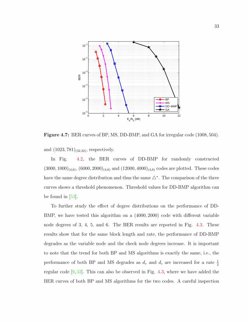
Figure 4.7: BER curves of BP, MS, DD-BMP, and GA for irregular code (1008, 504).
and (1023, 781)(32,32), respectively.
In Fig. 4.2, the BER curves of DD-BMP for randomly constructed
(3000, 1000)(4,6), (6000, 2000)(4,6) and (12000, 4000)(4,6) codes are plotted. These codes
have the same degree distribution and thus the same4∗. The comparison of the three
curves shows a threshold phenomenon. Threshold values for DD-BMP algorithm can
be found in [53].
To further study the effect of degree distributions on the performance of DD-
BMP, we have tested this algorithm on a (4000, 2000) code with different variable
node degrees of 3, 4, 5, and 6. The BER results are reported in Fig. 4.3. These
results show that for the same block length and rate, the performance of DD-BMP
degrades as the variable node and the check node degrees increase. It is important
to note that the trend for both BP and MS algorithms is exactly the same, i.e., the
performance of both BP and MS degrades as dv and dc are increased for a rate 12
regular code [9, 32]. This can also be observed in Fig. 4.3, where we have added the
BER curves of both BP and MS algorithms for the two codes. A careful inspection

34
of Fig. 4.3 shows that the performance gap between BP and MS on one hand and
DD-BMP on the other hand is decreased as (dv, dc) is increased from (4,8) to (5,10)
and (6,12). In fact, for the (6,12) code, the performance difference between MS and
DD-BMP reverses and DD-BMP outperforms MS. In Fig. 4.3, we have also presented
the BER for a (4000, 2000)(3,6) code under DD-BMP, BP and MS. It can be seen that
this degree distribution violates the trends just explained for DD-BMP. In particular,
the BER curve for this code demonstrates an early error flare. We have tested a
(8000, 4000)(3,6) code as well, and the same behavior is also observed for that code.
All the above observations closely follow the analytical analysis reported in [53] Table
II.
Finally, DD-BMP can also be applied to irregular LDPC codes. In Fig. 4.7, we
have provided the BER curves of DD-BMP, BP and MS for a (1008,504) irregular code
with the degree distribution optimized for BP and the code is constructed using the
modified PEG construction of [54]. As can be seen it has reduced the gap between
GA and BP algorithm. But at high bit error rates it is still 3 dB away from BP
algorithm. In terms of convergence DD-BMP needs a higher average number of
iterations in comparison to other decoding algorithms.
The average number of iterations vs. BER for BP, MS, DD-BMP and MB al-
gorithms are given in Figures 4.8 to 4.13 for all codes. These figures show that the
average number of iterations for DD-BMP is in general larger than those of the other
algorithms. The difference however is smaller, and in the cases of (1057, 813)(3,13) and
(273, 191)(17,17) is negligible, for lower BER values.
WBF algorithms and their variants and modifications [30, 34, 35, 39] have proved

35
10−8
10−6
10−4
10−2
100
0
10
20
30
40
50
60
70
80
90
BER
Ave
rage
Num
ber
of It
erat
ions
BP 3000BP 12000MS 3000MS12000DD−BMP 3000DD−BMP 6000DD−BMP 12000GA 3000GA 12000
Figure 4.8: Average number of iterations vs. BER for BP, MS, DD-BMP and GAfor code (3000, 1000)(4,6), (6000, 2000)(4,6) and (12000, 4000)(4,6).
10−8
10−6
10−4
10−2
100
0
10
20
30
40
50
60
70
80
BER
Ave
rage
Num
ber
of It
erat
ions
BP(6,12)BP(5,10)BP(4,8)MS(6,12)MS(5,10)MS(4,8)DD−BMP(6,12)DD−BMP(5,10)DD−BMP(4,8)GA(6,12)
Figure 4.9: Average number of iterations vs. BER for BP, MS, DD-BMP and GAfor code (4000, 2000) with different degree distributions.

36
10−8
10−6
10−4
10−2
100
0
5
10
15
20
25
BER
Ave
rage
Num
ber
of It
erat
ions
BPMSDD−BMPGA
Figure 4.10: Average number of iterations vs. BER for BP, MS, DD-BMP, and GAfor code (1057, 813)(3,13).
10−6
10−4
10−2
100
0
2
4
6
8
10
12
14
16
18
20
BER
Ave
rage
Num
ber
of It
erat
ions
BPMSIMWBFDD−BMPMDD−BMP
MB3
Figure 4.11: Average number of iterations vs. BER for BP, MS, IMWBF, DD-BMP,MDD-BMP and GA for code (273, 191)(17,17).

37
10−6
10−4
10−2
100
0
10
20
30
40
50
60
BER
Ave
rage
Num
ber
of It
erat
ions
BPMSIMWBFDD−BMPMDD−BMP
MB5
Figure 4.12: Average number of iterations vs. BER for BP, MS, IMWBF, DD-BMP,MDD-BMP and GA for code (1023, 781)(32,32).
10−6
10−5
10−4
10−3
10−2
10−1
100
0
5
10
15
20
25
30
35
40
45
50
BER
Ave
rage
Num
ber
of It
erat
ions
BPMSDD−BMPGA
Figure 4.13: Average number of iterations vs. BER for BP, MS, DD-BMP, and GAfor irregular code (1008, 504).

38
to perform well for decoding FG codes. The best performing algorithm in this cate-
gory is the improved modified WBF (IMWBF) algorithm of [35]. The performance of
this algorithm is given in Figures 4.5 and 4.6 for (273, 191)(17,17) and (1023, 781)(32,32),
respectively. As can be seen, IMWBF slightly outperforms DD-BMP by about 0.4 dB
and 0.2 dB for (273, 191)(17,17) and (1023, 781)(32,32), respectively. This improvement in
performance however is counter-balanced by the much larger average number of itera-
tions as illustrated in Figures 4.11 and 4.12, for (273, 191)(17,17) and (1023, 781)(32,32),
respectively. It is also important to note that all the stored and computed values
in IMWBF are floating-point real numbers. One would expect the performance to
deteriorate for a fixed-point implementation of IMWBF. For random codes, DD-BMP
usually outperforms IMWBF handily. From the computational complexity point of
view, IMWBF requires about 2E real comparisons, E real additions and N real mul-
tiplications for preprocessing before each iterative decoding to compute the reliability
information of check nodes and the initial values of the flipping functions. During
each iteration, IMWBF needs about dv × dc real additions and N real comparisons.
It also requires 2M real memory elements to store the reliability information of the
check nodes.
It is worth mentioning that we have also tried simplified variants of DD-BMP
algorithm. In particular we have tested a version of the algorithm where the memory
update operation of Eq. (4.2) is modified to
B(`)vi,cj
= B(`−1)vi,cj
+ sgn
( ∑ck∈N (vi)\cj
m(`)ck→vi
)(4.6)
It should be noted that Eq. (4.6) reduces to Eq. (4.2) for dv = 3. In general,
the performance of this algorithm appears to be only slightly inferior to that of the
original algorithm. The advantage however is the lower complexity as the operation
in Eq. (4.6) can be performed by a count up/down of the memory.

39
Another variant of the algorithm is to assign a memory to each variable node
instead of each edge in the graph and update its content in every iteration based on
the binary messages of the check nodes. The outgoing messages from a variable node
are all identical and are the sign of the memory content. This algorithm is simpler
and requires less memory but the performance for random codes is considerably worse
than that of the original algorithm. For FG codes the performance loss is smaller as
can be seen in Figures 4.5 and 4.6. In these figures the performance of this algorithm is
labeled as MDD-BMP, brief for modified DD-BMP. The average number of iterations
vs. BER for MDD-BMP is also given in Figures 4.11 and 4.12. As can be seen,
at lower BER values, MDD-BMP has a slight advantage over DD-BMP in terms of
average number of iterations.
Chapter 5
Adaptive Belief Propagation Decoding of
LDPC Codes
An adaptive control technique, originally presented by Kocarev et al. [36] to improve
the performance of turbo codes in the waterfall region, is applied to low-density
parity-check (LDPC) codes. For typical finite-length LDPC codes, the application of
the proposed technique improves the performance of belief propagation (BP) by up
to about 0.5 dB in the waterfall region. The proposed technique also improves the
performance of BP in the error floor region significantly. This is in contrast with the
results for turbo codes, where the technique appears to have no effect on the error
floor. We also show that the technique is robust against the changes of the channel
signal-to-noise ratio (SNR) and that the same control parameters can be used over a
wide range of SNR values with negligible performance degradation.
Belief propagation (BP) is widely used for decoding low-density parity-check
(LDPC) [1] and turbo [55] codes. Applied to cycle free graphs, which represent
codes with infinite block length, BP converges to a posteriori probabilities for bits.
For practical codes, where the graph representation has many small cycles, BP, al-
though still performing very well, becomes suboptimal [11]. The sub-optimality can
40

41
be attributed to the over-estimation of the reliability of messages [11], and the per-
formance of BP for finite-length codes can be enhanced by scaling or offsetting down
the reliability of messages [11,56,57].
Inspired by the representation of iterative decoding algorithms as nonlinear dy-
namical systems, Kocarev et al. proposed an alternate technique to improve the
performance of BP for finite-length turbo codes [36], [58]. The technique, which is
based on the adaptive control of transient chaos, is capable of improving the per-
formance of turbo decoders by 0.2 to 0.3 dB in the waterfall region [36], [58]. The
performance in the error floor region however remains unaffected. This is justified
by the lack of transient chaos in this region [36]. While the technique of [36, 58] is
similar to those proposed in [11,56] and [57] as it also aims at reducing the reliability
of messages, it also differs from them in that the reduction in reliability of a message
is achieved adaptively by a correction factor which is a function of the message itself.
LDPC codes, although similar to turbo codes in that they also belong to the
category of iterative coding schemes, sometimes demonstrate behaviors very different
than those of turbo codes. One example is the application of successive relaxation
(SR) to the iterative decoding of LDPC and turbo codes. While for turbo codes, SR
does not provide any improvement over the conventional successive substitution (SS)
[41], for LDPC codes significant improvements are observed [13]. We demonstrate
another example of different behavior of turbo codes and LDPC codes in this thesis.
We apply the adaptive control technique of [36,58] to the BP decoding of LDPC codes.
Using simulations, we demonstrate performance improvements of about 0.5 dB in the
waterfall region for the tested LDPC codes. Moreover, our results show significant
performance improvement in the error floor region. This is in stark contrast with the
results of turbo codes [36, 58], where the technique has almost no effect on the error
floor. This motivates us to analyze the performance of the technique in the error
floor region. To carry out the analysis, we use the a posteriori average entropy [36] as

42
a simple representation of decoding trajectories, and show that the improvement in
the error floor performance is a direct result of improvement in the chaotic transient
behavior of the decoder.
5.1 System Model and the Adaptive Control Tech-
nique
Consider the application of a binary LDPC code C over a binary-input AWGN channel
such that coded bits 0 and 1 are mapped to the channel input symbols +1 and -1,
respectively. Assume that C has length N and is described by an M ×N parity check
matrix H = [Hmn]. For a regular (dv, dc) code, parameters dv and dc represent the
number of ones in each column and each row of H, respectively. They also represent
the degrees of variable and check nodes in the Tanner graph [27] of C, respectively.
For irregular codes, not all the rows or all the columns have the same weight.
Suppose that the channel output yi corresponding to the transmitted symbol xi
is given by yi = xi + ni, where ni is a zero-mean Gaussian noise with variance σ2
independent of xi. Assuming that the AWGN has a power spectral density N0/2,
we have σ2 = 1/(2REb/N0), where Eb and R denote the energy per information bit
and the code rate, respectively. We consider a parallel BP decoder implemented in
the log-likelihood ratio (LLR) domain. The input to the decoder for the ith bit is
the channel LLR 2yi/σ2 . The decoder performs iterations until it converges to a
codeword or a maximum number of iterations Imax is reached.
To apply the adaptive control technique, we replace the outgoing messages mv→c
of variable nodes in the original BP algorithm by [36,58]
m′v→c = αmv→ce−β|mv→c| (5.1)

43
-300 -200 -100 0 100 200 300-40
-20
0
20
40
mV->C
m' V
->C
Figure 5.1: An example of Eq. (5.1).
The control function is chosen because if xi is small, then the attenuation factor
in (5.1) is close to 1 (since α is close to 1 and β is small). In other words, the
control algorithm does nothing. If, however, xi is large, then the control algorithm
reduces the normalization factor, thereby attenuating the effect of xi on the decoding
algorithm. Fig. 5.1 shows a realization of Eq. (5.1), as can be seen in this figure the
function’s slope for small values is close to 1.
where v and c are a pair of neighboring variable and check nodes, respectively,
and parameters α and β are constants selected from the intervals (0, 1] and [0,+∞),
respectively, to optimize the error rate performance of the algorithm. The optimal
values of α and β are usually close to the end and the beginning of the corresponding
intervals, respectively. It should be noted that the normalized BP algorithm of [11]
is a special case of Eq. (5.1) with β = 0, i.e., no adaptation. We have also applied
the adaptation to the output of check nodes as well as both the outputs of variable
nodes and check nodes. In both cases, the results are similar to the results reported

44
here.
5.2 Simulation Results and Analysis
To study the effects of the adaptive control technique on the BP decoding of finite-
length LDPC codes, we consider an optimized (1268,456) irregular code, also used
in [11], and a regular (504,252) code from [48]. For all the simulations, the maximum
number of iterations is set to 200 and for each simulation point, 100 codeword errors
are generated.
For the (1268,456) and (504,252) codes, the optimal values of α and β, which
minimize the bit error rate (BER), are found to be 1 and 0.008, and 0.99 and 0.010,
respectively. These values which are obtained by exhaustive search at Eb/N0 = 2.5
dB and 4 dB for the two codes, respectively, remain close-to-optimal over a wide
range of SNR values of interest. Fig. 5.2 shows BER curves of both codes decoded
by the original BP, and BP with adaptive control. We have also included in Fig. 5.2
the BER curves for normalized BP. The value of a for normalized BP, optimized for
the (1268,456) and (504,252) codes at Eb/N0 = 2.5 dB and 4 dB, is 0.9 and 0.75,
respectively. As can be seen, BP with adaptive control outperforms standard BP by
about 0.25 dB to 0.6 dB for BER values in the range of 10−7 − 10−6. Adaptive BP
also outperforms non-adaptive normalized BP. In particular, for the (1268,456) code,
the error floor performance of the former is superior to the latter. For the (504,252)
code, the performance improvement is mainly happening at lower SNR values. The
reason for this is the high sensitivity of the optimal value of α to the variations of SNR
for normalized BP. For example, for the (504,252) code while optimal α is 0.75 at
Eb/N0 = 4 dB, it increases to 0.95 at 2.0 dB. This sensitivity is substantially reduced
by the introduction of adaptive control in the algorithm of Eq. (5.1).
Fig. 5.3 compares the average number of iterations of the original BP, BP with

45
adaptive control and normalized BP versus BER for the two codes. The figure shows
that the improvement in performance for adaptive BP comes at no cost in the av-
erage number of iterations. In fact, for lower SNR values, adaptive BP requires a
smaller average number of iterations to converge compared to Normalized BP for
both codes. Compared to standard BP, there is an improvement at low SNR region
for the (504,252) code.
To analyze the superior performance of adaptive BP, we use the a posteriori av-
erage entropy defined by [36]
E(i) = − 1
N
N∑j=1
(p0j(i) log2 p0j(i) + p1j(i) log2 p
1j(i))
where i is the iteration number, and pkj (i), k ∈ {0, 1} is the a posteriori probability
of the jth bit being equal to k in iteration i. Although E(i) is probably too simple
to provide a comprehensive picture of the dynamical behavior of the decoder, its
evolution with i can be effectively used to identify the type of error events in which
the decoder is trapped. When the decoder converges to the right codeword, we
have E = 0. Fig. 5.4(b) shows the steady-state evolution of E(i + 1) vs. E(i) for
three instances of iterative decoding, which we associate with fixed-pattern, periodic-
pattern and random-like or chaotic error events. For the three instances, the number
of decoding errors versus the iteration number is also plotted in Fig. 5.4(a).
To analyze the difference in performance of standard BP and adaptive BP at
the high SNR region, we examine and categorize the failures of both algorithms and
track the changes with the increase in the maximum number of iterations Imax. In
particular, for the (1268,456) code and the (504,252) code, we present the results at
Eb/N0 = 2.5 dB, 2.75 dB, 3 dB, and 3.5 dB, 4 dB, 4.5 dB, in Tables 5.1 and 5.2,

46
1.5 2 2.5 3 3.510
-8
10-7
10-6
10-5
10-4
10-3
10-2
Eb/N0 (dB)
BER
a) (1268,456) Code
BP
Norm alized BP
Adaptive BP
2 2.5 3 3.5 4 4.5 510
-8
10-7
10-6
10-5
10-4
10-3
10-2
10-1
100
Eb/N0 (dB)
BER
b) (504,252) Code
BP
Normalized BP
Adaptive BP
Figure 5.2: BER for a) (1268,456) and b) (504,252) LDPC codes decoded by stan-dard BP, Normalized BP, and adaptive BP algorithms.
10-8
10-6
10-4
10-2
5
10
15
20
25
30
35
40
BER
Average Num
ber of Iterations
a) (1268,456) Code
BPNormalized BP
Adaptive BP
10-8
10-6
10-4
10-2
0
5
10
15
20
25
BER
Average Num
ber of Iterations
b) (504,252) Code
BPNormalized BP
Adaptive BP
Figure 5.3: Average number of iteration versus BER for a) (1268,456) and b)(504,252) LDPC codes decoded by standard BP, Normalized BP, and adaptiveBP algorithms.
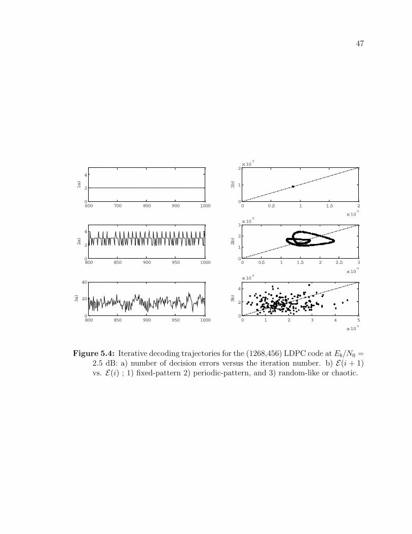
47
600 700 800 900 10000
2
4
1a)
0 0.5 1 1.5 2
x 10-3
0
1
2x 10
-3
1b)
800 850 900 950 10000
2
4
2a)
0 0.5 1 1.5 2 2.5 3
x 10-3
0
1
2
3x 10
-3
2b)
800 850 900 950 10000
20
40
3a)
0 1 2 3 4 5
x 10-3
0
2
4
x 10-3
3b)
Figure 5.4: Iterative decoding trajectories for the (1268,456) LDPC code at Eb/N0 =2.5 dB: a) number of decision errors versus the iteration number. b) E(i + 1)vs. E(i) ; 1) fixed-pattern 2) periodic-pattern, and 3) random-like or chaotic.
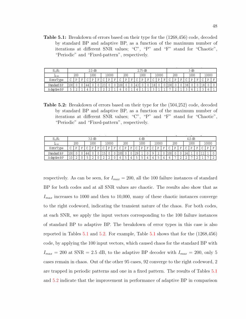
48
Table 5.1: Breakdown of errors based on their type for the (1268,456) code, decodedby standard BP and adaptive BP, as a function of the maximum number ofiterations at different SNR values; “C”, “P” and “F” stand for “Chaotic”,“Periodic” and “Fixed-pattern”, respectively.
p p yEb/N0 2.5 dB 2.75 dB 3 dBImax 200 1000 10000 200 1000 10000 200 1000 10000
Error Type C P F C P F C P F C P F C P F C P F C P F C P F C P FStandard BP 100 0 0 44 0 0 23 0 0 100 0 0 43 0 0 18 0 0 100 0 0 38 0 0 18 0 0Adaptive BP 5 2 1 4 2 1 2 2 1 6 0 1 4 1 1 3 1 1 7 2 1 3 6 1 3 6 1
Table 5.2: Breakdown of errors based on their type for the (504,252) code, decodedby standard BP and adaptive BP, as a function of the maximum number ofiterations at different SNR values; “C”, “P” and “F” stand for “Chaotic”,“Periodic” and “Fixed-pattern”, respectively.
; , , p , p yEb/N0 3.5 dB 4 dB 4.5 dBImax 200 1000 10000 200 1000 10000 200 1000 10000
Error Type C P F C P F C P F C P F C P F C P F C P F C P F C P FStandard BP 100 0 0 44 0 0 15 0 0 100 0 0 29 1 0 9 2 0 100 0 0 24 1 0 11 1 0Adaptive BP 10 2 0 5 2 0 2 2 0 6 5 4 5 5 4 4 5 4 6 7 2 2 7 2 1 7 2
respectively. As can be seen, for Imax = 200, all the 100 failure instances of standard
BP for both codes and at all SNR values are chaotic. The results also show that as
Imax increases to 1000 and then to 10,000, many of these chaotic instances converge
to the right codeword, indicating the transient nature of the chaos. For both codes,
at each SNR, we apply the input vectors corresponding to the 100 failure instances
of standard BP to adaptive BP. The breakdown of error types in this case is also
reported in Tables 5.1 and 5.2. For example, Table 5.1 shows that for the (1268,456)
code, by applying the 100 input vectors, which caused chaos for the standard BP with
Imax = 200 at SNR = 2.5 dB, to the adaptive BP decoder with Imax = 200, only 5
cases remain in chaos. Out of the other 95 cases, 92 converge to the right codeword, 2
are trapped in periodic patterns and one in a fixed pattern. The results of Tables 5.1
and 5.2 indicate that the improvement in performance of adaptive BP in comparison

49
with standard BP in the high Imax region is mainly due to the reduction in the chaotic
transient behavior. This effect is particularly prevalent for smaller values of Imax.

Chapter 6
Conclusions and Future Work
In this thesis we have studied iterative decoding algorithms and methods to improve
their performance. The main conclusions and proposed future work for each problem
are summarized below.
• Belief Propogation algorithm due to the existence of cycles in the Tanner graph
of practical codes is suboptimal. Improving the performance of BP is possi-
ble by normalizing the messages passed from variable nodes to check nodes in
the iterative decoder. We have proposed an adaptive normalization scheme to
improve the performance of BP algorithm.
• Inspired by the dynamics of SR, we propose a binary message-passing algorithm
for the decoding of LDPC codes. Similar to SR, the proposed algorithm is with
memory and the memory elements are updated differentially in each iteration
according to the binary messages. The proposed algorithm is able to close a large
portion of the gap between purely hard- decision and soft-decision algorithms.
• Successive Relaxation (SR) implementation of MS algorithm has shown to
achieve better bit error rates in comparison to conventional Successive Substitu-
tion (SS) implementations of MS. In SR-MS algorithm, variable node massages
are updated according to a different trajectory. As a result SR-MS generally
50

51
requires more number of iterations to converge. A further study on behavior
of orbits of SR-MS and devising a scheme to speed up the convergence while
maintaining the performance seems promising.
• The proposed adaptive normalized BP algorithm improves the BER perfor-
mance in expense of mild added complexity. The adaptive scaling factor
αe−β|mv→c| was originally chosen in [36, 58] to speed up the convergence. But
there might be other non-linear scaling functions that can perform better. A
further search for discovering other alternative scaling functions makes an in-
teresting research topic.

List of References
[1] R. Gallager, “Low-density parity-check codes,” IRE Trans. Inform. Theory,
vol. 8, pp. 21–28, 1962.
[2] D. MacKay and R. Neal, “Near Shannon limit performance of low density parity
check codes,” Electronics Letters, vol. 33, pp. 457 – 458, Aug. 1997.
[3] D. MacKay, “Good error-correcting codes based on very sparse matrices,” IEEE
Trans. Inform. Theory, vol. 45, pp. 399 – 431, March 1999.
[4] IEEE P802.3an, “1OGBASE-T task force,” http: //www. ieee8O2.org/3/an.
[5] IEEE 802.16e, “Air interface for fixed and mobile broadband wireless access
systems,” IEEE p802.16e/d12 draft, Feb. 2005.
[6] IEEE 802.11n, “Wireless lan medium access control and physical layer specifi-
cations,” IEEE p802.11n/d3.07, March 2008.
[7] “T.T.S.I. digital video broadcasting (DVB) second generation framing struc-
ture for broadband satellite applications,” http://www.dvb.org.
[8] M. Fossorier, M. Mihaljevic, and H. Imai, “Reduced complexity iterative decod-
ing of low-density parity check codes based on belief propagation,” IEEE Trans.
Commun., vol. 47, pp. 673 – 680, May 1999.
[9] J. Chen, A. Dholakia, E. Eleftheriou, M. Fossorier, and X.-Y. Hu, “Reduced-
complexity decoding of LDPC codes,” IEEE Trans. Commun., vol. 53, pp. 1288
– 1299, July 2005.
[10] M. Fossorier, “Iterative reliability-based decoding of low-density parity check
code,” IEEE J. Select. Areas Commun., vol. 19, pp. 908 – 917, May 2001.
[11] M. Yazdani, S. Hemati, and A. Banihashemi, “Improving belief propagation on
graphs with cycles,” IEEE Comm. Letters, vol. 8, pp. 57 – 59, Jan. 2004.
52

53
[12] Y. Mao and A. Banihashemi, “Decoding low-density parity-check codes with
probabilistic scheduling,” IEEE Commun. Letters, vol. 5, pp. 414 – 416, Oct.
2001.
[13] S. Hemati and A. Banihashemi, “Dynamics and performance analysis of analog
iterative decoding for low-density parity-check (LDPC) codes,” IEEE Trans. on
Commun., vol. 54, pp. 61 – 70, Jan. 2006.
[14] H. Xiao, S. Tolouei, and A. Banihashemi, “Successive relaxation for decoding of
LDPC codes,” in 24th Biennial Symposium on Communications, pp. 107 – 110,
June 2008.
[15] H. Xiao and A. H. Banihashemi, “Comments on successive relaxation for decod-
ing of LDPC codes,” IEEE Trans. on Comm., vol. 57, pp. 2846 – 2848, Oct.
2009.
[16] J. Proakis, Digital Communications. McGraw-Hill Series, 2000.
[17] S. Lin and D. Costello, Error Control Coding: Fundamentals And Applications.
Prentice-Hall, Englewood Cliffs, NJ, 2004.
[18] C. Shannon, “A mathematical theory of communication,” Bell System Technical
Journal, vol. 27, pp. 379 – 423, 623 – 656, July and October 1948.
[19] R. Hamming, “Error detecting and error correcting codes,” Bell Syst. Tech. J.,
vol. 29, pp. 147 – 160, April 1950.
[20] R. Bose and D. Ray-Chaudhuri, “On a class of error correcting binary group
codes,” Information and Control, vol. 3, pp. 68 – 79, March 1960.
[21] A. Hocquenghem, “Codes correcteurs derreurs,” Chiffres, vol. 2, pp. 147 – 156,
September 1959.
[22] I. Reed, , and G. Solomon, “Polynomial codes over certain finite fields,” Journal
of the Society for Industrial and Applied Mathematics, vol. 8, pp. 300 – 304, June
1960.
[23] P. Elias, “Coding for noisy channels,” IRE Conv. Rec., vol. 4, pp. 37–46, Sept.
1955.
[24] A. Viterbi, “Error bounds for convolutional codes and an asymptotically opti-
mum decoding algorithm,” IEEE Trans. on Inform. Theory, vol. IT-13, pp. 260–
269, February 1967.

54
[25] R. Gallager, Low-Density Parity-Check Codes. PhD thesis, Cambridge, MA:
MIT Press, 1963.
[26] R. Blahut, Theory and Practice of Error Control Codes. Addison-Weseley Pub-
lishing Co., 1984.
[27] R. Tanner, “A recursive approach to low complexity codes,” IEEE Trans. Inform.
Theory, vol. 27, pp. 533 – 547, Sept. 1981.
[28] M. Davey and D. MacKay, “Low-density parity check codes over GF(q),” IEEE
Comm. Letters, vol. 2, pp. 165 – 167, June 1998.
[29] D. MacKay, “Gallager codes that are better than Turbo codes,” in in Proc. 36th
Allerton Conf. Communication, Control, and Computing, Monticello, IL, Sept.
1998.
[30] Y. Kou, S. Lin, and M. Fossorier, “Low-density parity-check codes based on
finite geometries: a rediscovery and new results,” IEEE Trans. Inform. Theory,
vol. 47, pp. 2711 – 2736, Nov. 2001.
[31] P. Zarrinkhat and A. Banihashemi, “Threshold values and convergence proper-
ties of majority-based algorithms for decoding regular low-density parity-check
codes,” IEEE Trans. Commun., vol. 52, pp. 2087 – 2097, Dec. 2004.
[32] T. Richardson and R. Urbanke, “The capacity of low-density parity-check codes
under message-passing decoding,” IEEE Trans. Inform. Theory, vol. 47, pp. 599
– 618, Feb. 2001.
[33] H. Xiao and A. H. Banihashemi, “Graph-based message-passing schedules for
decoding LDPC codes,” IEEE Trans. Comm., vol. 52, pp. 2098 – 2105, Dec.
2004.
[34] J. Zhang and M. Fossorier, “A modified weighted bit-flipping decoding of low-
density parity-check codes,” IEEE Commun. Letters, vol. 8, pp. 165 – 167, March
2004.
[35] M. Jiang, C. Zhao, Z. Shi, and Y. Chen, “An improvement on the modified
weighted bit flipping decoding algorithm for LDPC codes,” IEEE Communica-
tions Letters, vol. 9, pp. 814 – 816, Sept. 2005.
[36] L. Kocarev, F. Lehmann, G. Maggio, B. Scanavino, Z. Tasev, and A. Vardy,
“Nonlinear dynamics of iterative decoding systems: Analysis and applications,”
IEEE Trans. Inform. Theory, vol. 52, pp. 1366 – 1384, April 2006.

55
[37] S. Hemati, Iterative Decoding in Analog VLSI. PhD thesis, Ottawa-Carleton
Institute For Electrical and Computer Engineering, 2005.
[38] T. K. Moon and W. C. Stirling, Mathematical Methods and Algorithms for Signal
Processing. Prentice Hall, 1999.
[39] Z. Liu and D. A. Pados, “A decoding algorithm for finite-geometry LDPC
codes,” IEEE Trans. Comm., vol. 53, pp. 415 – 421, April 2005.
[40] T. M. N. Ngatched, F. Takawira, and M. Bossert, “A modified bit-flipping decod-
ing algorithm for low-density parity-check codes,” in IEEE International Con-
ference on Commun. ICC ’07, pp. 653 – 658, August 2007.
[41] P. Moqvist and T. M. Aulin, “Turbo-decoding as a numerical analysis problem,”
in Information Theory, 2000. Proceedings. IEEE International Symposium on,
p. 485, June 2000.
[42] E. Yeo, P. Pakzad, B. Nikolic, and V. Anantharam, “High throughput low-
density parity-check decoder architectures,” in IEEE Global Telecommunications
Conference, GLOBECOM ’01, vol. 5, pp. 3019 – 3024, Nov. 2001.
[43] J. Dielissen, A. Hekstra, and V. Berg, “Low cost LDPC decoder for DVB-S2,”
in DATE Designers’ Forum 2006, pp. 130 – 135, March 2006.
[44] J. Yedidia, W. Freeman, and Y. Weiss, “Constructing free-energy approximations
and generalized belief propagation algorithms,” IEEE Trans. on Inform. Theory,
vol. 51, pp. 2282 – 2312, July 2005.
[45] S. Hemati and A. Banihashemi, “On the dynamics of continuous-time analog
iterative decoding,” in IEEE International Symposium on Information Theory,
ISIT ’04, p. 262, June 2004.
[46] A. Amat, S. Benedetto, G. Montorsi, D. Vogrig, A. Neviani, and A. Gerosa,
“Design, simulation, and testing of a CMOS analog decoder for the block length-
40 UMTS Turbo code,” IEEE Trans. Comm., vol. 54, pp. 1973 – 1982, Nov.
2006.
[47] Y. Mao and A. Banihashemi, “A heuristic search for good low-density parity-
check codes at short block lengths,” in IEEE International Conference on Com-
munications, ICC 2001, vol. 1, pp. 41 – 44, June 2001.
[48] D. J. C. MacKay, “Encyclopedia of sparse graph codes [online],” in Available at:
http://www.inference.phy.cam.ac.uk/mackay/codes/data.html.
56
[49] N. Mobini, A. Banihashemi, and S. Hemati, “A differential binary message pass-
ing LDPC decoder,” in IEEE Global Telecommunications Conference, GLOBE-
COM ’07, pp. 1561 – 1565, Nov. 2007.
[50] N. Mobini, A. Banihashemi, and S. Hemati, “A differential binary message-
passing ldpc decoder,” IEEE Trans. on Commun., vol. 57, pp. 2518 – 2523,
Sept. 2009.
[51] A. J. Blanksby and C. J. Howland, “A 690-mW 1-Gb/s 1024-b, rate-1/2 low-
density parity-check code decoder,” IEEE J. Solid-State Circuits, vol. 37, pp. 404
– 412, March 2002.
[52] S. T. Brink, G. Kramer, and A. Ashikhmin, “Design of low-density parity check
codes for modulation and detection,” IEEE Trans. Comm., vol. 52, pp. 670 –
678, April 2004.
[53] E. Janulewicz and A. Banihashemi, “Performance analysis of iterative decoding
algorithms with memory,” in IEEE Information Theory Workshop (ITW), pp. 1
– 5, Jan. 2010.
[54] H. Xiao and A. Banihashemi, “Improved progressive-edge-growth (PEG) con-
struction of irregular LDPC codes,” IEEE Comm. Letters, vol. 8, pp. 715 – 717,
Dec. 2004.
[55] C. Berrou, A. Glavieux, and P. Thitimajshima, “Near shannon limit error-
correcting coding and decoding: Turbo-codes,” in Technical program, confer-
ence record, IEEE international conference on Communications, ICC 93, vol. 2,
pp. 1064 –1070, May 1993.
[56] D. MacKay and M. Davey, “Evaluation of gallager codes for short block length
and high rate applications,” Codes, Systems and Graphical Models, vol. 123,
pp. 113–130, 1999.
[57] R. Lucas, M. Fossorier, Y. Kou, and S. Lin, “Iterative decoding of one-step
majority logic deductible codes based on belief propagation,” Communications,
IEEE Transactions on, vol. 48, pp. 931–937, June 2000.
[58] L. Kocarev, Z. Tasev, and A. Vardy, “Improving turbo codes by control of tran-
sient chaos in turbo-decoding algorithms,” Electronics Letters, vol. 38, pp. 1184
– 1186, Sep. 2002.
Recommended