Proceedings of the 5th NA International Conference on Industrial Engineering and Operations Management Detroit, Michigan, USA, August 10 - 14, 2020
© IEOM Society International
Multilevel Reorder Strategy-based Supply Chain Model
Hesamoddin Tahami, Hengameh Fakhravar Engineering Management & Systems Engineering Department
Old Dominion University Norfolk, VA 23529, USA
[email protected], [email protected]
Abstract We investigate the stochastic integrated inventory model wherein the buyer’s lead time demand follows the mixture of normal distributions. Due to the high acquisition cost of land, we assume that buyer’s maximum permissible storage space is limited and therefore adds a space constraint to the respective inventory system. Besides, it is assumed that the manufacturing process is imperfect and produces defective units, and hence each lot received by the buyer contains percentage defectives. The paper also considers controllable lead time components and ordering cost for the system. Based on lead-time components, a multilevel reorder strategy-based supply chain model is developed for the proposed system, and a Lagrange multiplier method is applied to solve the problem to reduce the expected inventory cost of both buyer and vendor. We develop a solution procedure to find the optimal values and show the applicability of the model and solution procedure in numerical examples. Keywords Integrated vendor-buyer model, Imperfect production, Stochastic lead time, Nonlinear constrained optimization, Mixture of normal distributions 1. Introduction The integrated inventory model of both buyer and vendor has been received a lot of attention in the past decade. Researchers have proposed that having better coordination of all parties involved in a supply chain will lead to benefit the entire supply network rather than a single company. (Goyal, 1977) and (Banerjee, 1986) were the first researchers that aim to obtain coordinated inventory replenishment decisions. In the mentioned studies, demand and lead time were assumed to be deterministic. However, demand or lead time across different industries is distributed stochastically, so it is relevant and meaningful to consider uncertainty in integrated inventory models. Also, with the successful Japanese experience of using Just-In-Time (JIT) production, the benefits associated with controlling the lead time can be perceived. These benefits include lower safety stock, improve customer service level, and, thus, increase the competitiveness in the industry. To address this issue, researchers started to extend the previously established models by developing lead time reduction inventory models under various crashing cost functions. (Liao & Shyu, 1991) were the first researchers to introduce variable lead times in the inventory model. In their model, they assumed that to reduce the lead time to a specified minimum duration, lead time could be decomposed into several components with different crashing costs. Since then, many researchers have made significant contributions to controllable lead-time literature. ((Ouyang et al., 2004), (Tahami et al., 2019)). Ordering cost reduction has become an essential aspect of business success and has recently attracted considerable research attention. It can be shown that ordering cost control can affect directly or indirectly the ordering size, service level, and business competitiveness. Integrated vendor-buyer inventory models were typically developed to consider fixed ordering costs. However, in some practical situations, the cost of ordering can be controlled and reduced in various ways. It can be achieved through workforce training, process changes, and special equipment acquisition. (Porteus, 1985) was the first researcher proposed an inventory model considering an investment in reducing set up cost. (Chang et al., 2006) suggested that in addition to controllable lead time, ordering cost could also be considered as a controllable variable. They proposed that the buyer ordering cost could be reduced by the additional crashing cost, which could be defined as a function of lead time length and ordering lot size. Later, other researchers developed setup/order cost reduction inventory models under various assumptions. ((Lou & Wang, 2013), (Tahami et al., 2016)) Assuming that buyer possesses infinite storage capacity is not realistic. In contrast, most probably, the buyer storage capacity is limited. Most previous research on space-constrained inventory problems focused on deterministic demand
1319
Proceedings of the 5th NA International Conference on Industrial Engineering and Operations Management Detroit, Michigan, USA, August 10 - 14, 2020
© IEOM Society International
having multiple items in the system (Haksever & Moussourakis, 2005), and few papers considered stochastic demand models. One of the first authors proposed inventory models with storage space constraint in the stochastic environment was (Veinott, 1965). (Hariga, 2010) proposed a single item stochastic inventory model with a random demand wherein buyer storage space was limited. In the proposed model, the order quantity and reorder point were considered as decision variables. (Moon & Ha, 2012) presented a multi-item EOQ model with limited storage space and random yields. They solved the model using the Lagrange multiplier method. In our proposed model, we employ the same Lagrange multiplier technique to solve the non-linear objective function. One of the assumptions of the inventory management literature is that the quality of the product in a lot is perfect. In practice, however, a received lot may contain some defective items. If there is a possibility that a lot contains defective items, the firm may issue a larger order than was originally planned to guarantee the satisfaction of customer demand. (Huang, 2002) proposed an integrated inventory policy for a vendor-buyer model wherein manufacturing process was imperfect and a lot transferred to the buyer contained a fixed fraction of defectives with known probability distribution function. In the previously discussed research, demand was assumed deterministic. However, demand is stochastically distributed in its nature in most industries ((Fazeli et al., 2020), (Yahoodik et al., 2020)). Very few papers have been published for stochastic demand integrated vendor buyer inventory models under defective items considerations. (Ho, 2009) investigated an integrated vendor-buyer inventory system with defective goods in the buyer’s arrival order lot. Utilizing the result of a basic theorem from renewal reward processes ((Ross, 1996)) and minimax distribution free procedure for unidentified lead time demand distribution, she obtained the minimum total expected annual cost. In the case of probabilistic demand, as can be seen in various industries, it is prevalent that the demands by the different customers are not identical, and the distribution of demand for each customer can be adequately approximated by a distribution. The overall distribution of demand is then mixture. So, we cannot use only a single distribution. (Lee et al., 2004) proposed a one-sided inventory system with defective goods wherein the lead time demand followed a mixture of normal distributions and found buyer’s optimal inventory strategy when reorder point, lead time, and ordering quantity were the decision variables. In the previously mentioned research, one facility (e.g., a buyer) is assumed to minimize its own cost. This one-sided-optimal- strategy is not appropriate for the global market. Therefore, in this study, we consider a mixture of normally distributed lead time demand for integrated single-vendor single-buyer inventory model rather one facility. Also, the present paper extends the mentioned works for a multi-reorder level inventory system based on lead time components. Besides, we assume that the lead time is controllable and transportation and setup times and their crashing cost act independently. Also, in order to fit some real environment, transportation time crashing cost is presented as a function of reduced transportation time and the quantities in the orders. In this paper, a random space constraint for random demand and positive lead time is considered when maximum permissible storage space is restricted. Also, the manufacturing process is considered imperfect, and defective items are found in the buyer inspection process. The objective is to minimize joint inventory expected cost by simultaneously optimizing ordering quantity, reorder points of different batches, ordering cost, setup time, transportation time, production time and a number of deliveries under imperfect production process and buyer space constraint while the lead time demand follows a mixture of normal distributions. The Lagrangian method is applied to solve the problem. The rest of the paper is organized as follows. In section 2, the notations and assumptions are given. In section 3, we present the mathematical model. In section 4, a numerical example and sensitivity analysis are provided to illustrate the model and its solution procedure. Finally, we conclude the paper. 2. Notations and assumptions 2.1 Notations Following notations have been used through the paper: 𝑄𝑄 Buyer’s order quantity, as a decision variable 𝑟𝑟 Buyer’s Reorder point, as a decision variable 𝐴𝐴 Buyer’s ordering cost at the time zero, as a decision variable 𝑡𝑡 Transportation time, as a decision variable 𝑠𝑠 Setup time, as a decision variable 𝑚𝑚 The number of lots in which the product is delivered from the vendor to the buyer in one Production cycle, a positive integer, as a decision variable 𝛾𝛾 Defective rate in an order lot, 𝛾𝛾𝛾𝛾[0,1) and is a random variable
1320

Proceedings of the 5th NA International Conference on Industrial Engineering and Operations Management Detroit, Michigan, USA, August 10 - 14, 2020
© IEOM Society International
𝑔𝑔(𝛾𝛾) Probability density function (p.d.f.) of 𝛾𝛾 𝐷𝐷 Annual demand for buyer 𝑃𝑃 Production rate in units per unit time 𝑝𝑝 1 𝑃𝑃⁄ 𝑎𝑎 Vendor’s setup cost per set up at the time zero 𝜋𝜋 Buyer’s stock out cost per unit at the time zero ℎ𝑣𝑣 Vendor’s holding cost per item per year at the time zero ℎ𝑏𝑏1 Buyer’s holding cost per non-defective item per unit time ℎ𝑏𝑏2 Buyer’s holding cost per defective item per year at the time zero 𝜆𝜆 Screening rate 𝑆𝑆𝑐𝑐 Unit screening cost 𝑊𝑊𝑐𝑐 Vendor’s unit treatment cost (include warranty cost) of defective items 𝑓𝑓 Space used per unit 𝐹𝐹 Maximum permissible storage space 𝐼𝐼(𝐴𝐴) Buyer’s capital investment required to achieve ordering cost 𝐴𝐴, 0 < 𝐴𝐴 ≤ 𝐴𝐴0 𝑏𝑏 Percentage decrease in ordering cost A per dollar increase in investment 𝐼𝐼(𝐴𝐴) 𝜃𝜃 Fractional opportunity cost of capital investment per year 𝐶𝐶𝑝𝑝𝑝𝑝 Buyer’s purchasing cost per unit at the time zero 𝑐𝑐𝑠𝑠 Vendor’s Setup cost per setup at the time zero 𝑐𝑐𝑝𝑝𝑝𝑝 Vendor’s Production cost per unit at the time zero 𝐴𝐴0 Buyer’s original ordering cost per order 𝑋𝑋 Demand during lead time, as a random variable 𝑋𝑋+ Maximum value of x and 0 𝐸𝐸(∙) Mathematical expectation 2.2 Assumptions 1. A single-vendor and single-buyer for a single product are considered in this paper. 2. The vendor’s production rate for the perfect items is finite and greater than the buyer’s demand rate, i.e., 𝑃𝑃(1 −𝑀𝑀𝛾𝛾) > 𝐷𝐷, where 𝑀𝑀𝛾𝛾, 𝑃𝑃 and 𝐷𝐷 are given. 3. The buyer orders a lot of size 𝑚𝑚𝑄𝑄, and the vendor manufactures a lot of size 𝑚𝑚𝑄𝑄, but transfer a shipment of size 𝑄𝑄 to the buyer. Once the vendor produces the first 𝑄𝑄 units, he will deliver them to the buyer. After the first delivery and buyer’s inspection, the vendor will schedule successive deliveries every 𝑄𝑄(1−𝑀𝑀𝛾𝛾)
𝐷𝐷 units of time.
4. An arrival lot, 𝑄𝑄, may contain some defective goods and the proportion defective, 𝛾𝛾, is a random variable which has a PDF, 𝑓𝑓(𝛾𝛾), with finite mean 𝑀𝑀𝛾𝛾 and variance 𝑉𝑉𝛾𝛾. Upon the arrival of an order, all the items are inspected (the screen rate is 𝜆𝜆) by the buyer, and defective items in each lot will be discovered and returned to the vendor at the time of delivery of the next lot. Hence, the buyer will have two extra costs: inspection cost and defective items holding cost. 5. During the screening period, the on-hand non-defective inventory is larger or equal to the demand. 6. We assume that the capital investment, 𝐼𝐼(𝐴𝐴), in reducing buyer’s ordering cost is a logarithmic function of the ordering cost 𝐴𝐴. That is,
𝐼𝐼(𝐴𝐴) =1𝛿𝛿𝑙𝑙𝑙𝑙 �
𝐴𝐴0𝐴𝐴� 𝑓𝑓𝑓𝑓𝑟𝑟 0 < 𝐴𝐴 ≤ 𝐴𝐴0
Where 𝛿𝛿 is the fraction of the reduction in 𝐴𝐴 per dollar increase in investment. 7. Setup time 𝑠𝑠 consists of 𝑙𝑙𝑠𝑠 mutually independent components. The ith component has a normal duration 𝑁𝑁𝑆𝑆𝑖𝑖 and minimum duration 𝑀𝑀𝑆𝑆𝑖𝑖 , 𝑖𝑖 = 1,2, … ,𝑙𝑙𝑠𝑠. If we let 𝑠𝑠0 = ∑ 𝑁𝑁𝑆𝑆𝑗𝑗𝑛𝑛𝑠𝑠
𝑗𝑗=1 and 𝑠𝑠𝑖𝑖 be the length of setup time with components 1,2,…,i, crashed to their minimum duration, then 𝑠𝑠𝑖𝑖 can be expressed as 𝑠𝑠𝑖𝑖 = ∑ 𝑁𝑁𝑆𝑆𝑗𝑗𝑛𝑛
𝑗𝑗=1 − ∑ �𝑁𝑁𝑆𝑆𝑗𝑗 −𝑀𝑀𝑆𝑆𝑗𝑗�𝑖𝑖𝑗𝑗=1 , 𝑖𝑖 =
1,2, … ,𝑙𝑙𝑠𝑠 and the setup time crashing cost is given by 𝐶𝐶𝑆𝑆(𝑠𝑠) = 𝑐𝑐𝑠𝑠𝑖𝑖(𝑠𝑠𝑖𝑖−1 − 𝑠𝑠) + ∑ 𝑐𝑐𝑠𝑠𝑗𝑗�𝑁𝑁𝑆𝑆𝑗𝑗 − 𝑀𝑀𝑆𝑆𝑗𝑗�𝑖𝑖−1
𝑗𝑗=1 . 8. The transportation time 𝑡𝑡 consists of 𝑙𝑙𝑡𝑡 mutually independent components. The ith component has a normal duration 𝑁𝑁𝑇𝑇𝑖𝑖 and minimum duration 𝑀𝑀𝑇𝑇𝑖𝑖 , 𝑖𝑖 = 1,2, … ,𝑙𝑙𝑡𝑡 .
1321

Proceedings of the 5th NA International Conference on Industrial Engineering and Operations Management Detroit, Michigan, USA, August 10 - 14, 2020
© IEOM Society International
9. For the ith component of transportation time, the crashing cost per unit time 𝑐𝑐𝑡𝑡𝑖𝑖, depends on the ordering lot size 𝑄𝑄 and is described by 𝑐𝑐𝑡𝑡𝑖𝑖 = 𝑎𝑎𝑖𝑖 + 𝑏𝑏𝑖𝑖𝑄𝑄 , where 𝑎𝑎𝑖𝑖 > 0 is the fixed cost, and 𝑏𝑏𝑖𝑖 > 0 is the unit variable cost, for 𝑖𝑖 =1,2, … ,𝑙𝑙𝑡𝑡 . 10. For any two crash cost lines 𝑐𝑐𝑡𝑡𝑖𝑖 = 𝑎𝑎𝑖𝑖 + 𝑏𝑏𝑖𝑖𝑄𝑄 and 𝑐𝑐𝑡𝑡𝑗𝑗 = 𝑎𝑎𝑗𝑗 + 𝑏𝑏𝑗𝑗𝑄𝑄 , where 𝑎𝑎𝑖𝑖 > 𝑎𝑎𝑗𝑗 , 𝑏𝑏𝑖𝑖 < 𝑏𝑏𝑗𝑗 , for 𝑖𝑖 ≠ 𝑗𝑗 and 𝑖𝑖, 𝑗𝑗 =1,2, … ,𝑙𝑙𝑡𝑡, there is an intersection point 𝑄𝑄𝑆𝑆 such that 𝑐𝑐𝑡𝑡𝑖𝑖 = 𝑐𝑐𝑡𝑡𝑗𝑗. These intersection points are arranged in ascending order so that 𝑄𝑄0𝑆𝑆 < 𝑄𝑄1𝑆𝑆 < ⋯ < 𝑄𝑄𝑤𝑤𝑆𝑆 < 𝑄𝑄𝑤𝑤+1𝑆𝑆 , where 𝑄𝑄0𝑆𝑆 = 0,𝑄𝑄𝑤𝑤+1𝑆𝑆 = ∞ and 𝑤𝑤 ≤ 𝑙𝑙𝑡𝑡(𝑙𝑙𝑡𝑡 − 1) 2⁄ . For any order quantity range (𝑄𝑄𝑖𝑖𝑆𝑆 ,𝑄𝑄𝑖𝑖+1𝑆𝑆 ), 𝑐𝑐𝑖𝑖𝑠𝑠 are arranged such that 𝑐𝑐1 ≤ 𝑐𝑐2 ≤ ⋯ ≤ 𝑐𝑐𝑛𝑛𝑡𝑡, and the lead time components are crashed one at a time starting with the component of least 𝑐𝑐𝑖𝑖, and so on. 11. Let 𝑡𝑡0 ≡ ∑ 𝑁𝑁𝑇𝑇𝑗𝑗𝑛𝑛𝑡𝑡
𝑗𝑗=1 and 𝑡𝑡𝑖𝑖 be the length of transportation time with components 1,2, … , 𝑖𝑖 crashed to their minimum duration, then 𝑡𝑡𝑖𝑖 can be expressed as 𝑡𝑡𝑖𝑖 = 𝑡𝑡0 − ∑ �𝑁𝑁𝑇𝑇𝑗𝑗 − 𝑀𝑀𝑇𝑇𝑗𝑗�𝑖𝑖
𝑗𝑗=1 , 𝑖𝑖 = 1,2, … ,𝑙𝑙𝑡𝑡 and the transportation time crashing cost per cycle 𝐶𝐶𝑇𝑇(𝑡𝑡) is given by 𝐶𝐶𝑇𝑇(𝑡𝑡) = 𝑐𝑐𝑡𝑡𝑖𝑖(𝑡𝑡𝑖𝑖−1 − 𝑡𝑡) + ∑ 𝑐𝑐𝑗𝑗(𝑁𝑁𝑇𝑇𝑗𝑗 −𝑀𝑀𝑇𝑇𝑗𝑗)𝑖𝑖−1
𝑗𝑗=1 , where 𝑡𝑡𝛾𝛾[𝑡𝑡𝑖𝑖, 𝑡𝑡𝑖𝑖−1], and 𝑐𝑐𝑗𝑗 = 𝑎𝑎𝑗𝑗 + 𝑏𝑏𝑗𝑗𝑄𝑄 for 𝑗𝑗 = 1,2, … , 𝑖𝑖. 12. We consider the deterministic lead time 𝐿𝐿 and assume that the demand for the lead time 𝑋𝑋 follows the mixture of normal distributions, 𝐹𝐹∗ = 𝛼𝛼𝐹𝐹1 + (1 − 𝛼𝛼)𝐹𝐹2 , where 𝐹𝐹1has a normal distribution with finite mean 𝜇𝜇1 and standard deviation 𝜎𝜎√𝐿𝐿 and 𝐹𝐹2has a normal distribution with finite mean 𝜇𝜇2 and standard deviation 𝜎𝜎√𝐿𝐿. Therefore, the lead time demand, 𝑋𝑋, has a mixture of probability density function (𝑃𝑃𝐷𝐷𝐹𝐹) which is given by
𝑓𝑓(𝑥𝑥) = 𝛼𝛼1
√2𝜋𝜋𝜎𝜎√𝐿𝐿× 𝑒𝑒𝑥𝑥𝑝𝑝 �−
12�𝑥𝑥 − 𝜇𝜇1𝐿𝐿𝜎𝜎√𝐿𝐿
�2
� + (1 − 𝛼𝛼)1
√2𝜋𝜋𝜎𝜎√𝐿𝐿× 𝑒𝑒𝑥𝑥𝑝𝑝 �−
12�𝑥𝑥 − 𝜇𝜇2𝐿𝐿𝜎𝜎√𝐿𝐿
�2
�
Where 𝜇𝜇1 − 𝜇𝜇2 = 𝑘𝑘1 𝜎𝜎 √𝐿𝐿⁄ or 𝜇𝜇1𝐿𝐿 − 𝜇𝜇2𝐿𝐿 = 𝑘𝑘1𝜎𝜎√𝐿𝐿 , 𝑘𝑘1 > 0 , −∞ < 𝑥𝑥 < ∞ , 0 ≤ 𝛼𝛼 ≤ 1 , 𝜎𝜎 > 0 . Moreover, the
mixture of normal distributions is unimodal for all 𝛼𝛼 if (𝜇𝜇1 − 𝜇𝜇2)2 < 27𝜎𝜎2 8𝐿𝐿⁄ or 𝑘𝑘1 < �278
. Also, when
(𝜇𝜇1 − 𝜇𝜇2)2 > 4𝜎𝜎2 𝐿𝐿⁄ or 𝑘𝑘1 > 2, at least we can find a value of 𝛼𝛼 (0 ≤ 𝛼𝛼 ≤ 1), which makes the mixture of normal distributions to be a bimodal distribution. 13. The reorder point 𝑟𝑟 = expected demand during lead time + safety stock (ss), and 𝑠𝑠𝑠𝑠 = 𝑘𝑘 × (standard deviation of lead time demand), that is 𝑟𝑟 = 𝜇𝜇∗𝐿𝐿 + 𝑘𝑘𝜎𝜎∗√𝐿𝐿 , where 𝜇𝜇∗ = 𝛼𝛼𝜇𝜇1 + (1 − 𝛼𝛼)𝜇𝜇2 , 𝜎𝜎∗ = �1 + 𝛼𝛼(1 − 𝛼𝛼)𝑘𝑘12𝜎𝜎 , 𝜇𝜇1 = 𝜇𝜇∗ +(1 − 𝛼𝛼)𝑘𝑘1𝜎𝜎 √𝐿𝐿⁄ , 𝜇𝜇2 = 𝜇𝜇∗ − 𝛼𝛼𝑘𝑘1𝜎𝜎 √𝐿𝐿⁄ , and 𝑘𝑘 is the safety factor which satisfies 𝑃𝑃(𝑋𝑋 > 𝑟𝑟) = 1 − 𝑝𝑝Φ(𝑟𝑟1) −(1 − 𝑝𝑝)Φ(𝑟𝑟2) = 𝑞𝑞, where Φ represents the cumulative distribution function of the standard normal random variable, 𝑞𝑞 represents the allowable stock-out probability during 𝐿𝐿, 𝑟𝑟1 = �𝑟𝑟 − 𝜇𝜇1𝐿𝐿 𝜎𝜎√𝐿𝐿⁄ � = �𝑟𝑟 − 𝜇𝜇∗𝐿𝐿 𝜎𝜎√𝐿𝐿⁄ � − (1 − 𝛼𝛼)𝑘𝑘1, and 𝑟𝑟2 = �𝑟𝑟 − 𝜇𝜇2𝐿𝐿 𝜎𝜎√𝐿𝐿⁄ � = �𝑟𝑟 − 𝜇𝜇∗𝐿𝐿 𝜎𝜎√𝐿𝐿⁄ � + 𝑘𝑘1𝛼𝛼. 14. Lead time for the first shipment is proportional to the lot size produced by the vendor and consists of the sum of setup, transportation and production time, i.e., 𝐿𝐿(𝑄𝑄, 𝑠𝑠, 𝑡𝑡) = 𝑠𝑠 + 𝑝𝑝𝑄𝑄 + 𝑡𝑡. For shipments 2,…,m only transportation time has to be considered for calculating lead time, i.e., 𝐿𝐿(𝑡𝑡) = 𝑡𝑡. Since, due to 𝑃𝑃 > 𝐷𝐷, shipments 2,…,m have been completed when the order of buyers arrives. Hence, considering a mixture of normal distributions, the lead time demand for the first batch, 𝑋𝑋1, has a probability density function 𝑓𝑓 �𝑥𝑥1, 𝜇𝜇1𝐿𝐿(𝑄𝑄, 𝑠𝑠, 𝑡𝑡), 𝜇𝜇2𝐿𝐿(𝑄𝑄, 𝑠𝑠, 𝑡𝑡),𝜎𝜎�𝐿𝐿(𝑄𝑄, 𝑠𝑠, 𝑡𝑡),𝛼𝛼�
with means 𝜇𝜇1𝐿𝐿(𝑄𝑄, 𝑠𝑠, 𝑡𝑡), 𝜇𝜇2𝐿𝐿(𝑄𝑄, 𝑠𝑠, 𝑡𝑡) and standard deviation 𝜎𝜎�𝐿𝐿(𝑄𝑄, 𝑠𝑠, 𝑡𝑡) and for the other batches, the lead time demand, 𝑋𝑋2, has a probability density function 𝑓𝑓 �𝑥𝑥2, 𝜇𝜇1𝐿𝐿(𝑡𝑡), 𝜇𝜇2𝐿𝐿(𝑡𝑡),𝜎𝜎�𝐿𝐿(𝑡𝑡),𝛼𝛼� with means 𝜇𝜇1𝐿𝐿(𝑡𝑡), 𝜇𝜇2𝐿𝐿(𝑡𝑡) and
standard deviation 𝜎𝜎�𝐿𝐿(𝑡𝑡). 3. Model formulation As mentioned in assumption 3, the buyer orders 𝑚𝑚𝑄𝑄 units, and the vendor delivers the order quantity of size 𝑄𝑄 to the buyer in 𝑚𝑚 batches. As stated in assumption 4, each received lot contains a defective percentage, 𝛾𝛾, of defective items which is a probabilistic variable with finite mean 𝑀𝑀𝛾𝛾 and variance 𝑉𝑉𝛾𝛾. Hence, the expected number of non-defective items in each shipment is �1 −𝑀𝑀𝛾𝛾�𝑄𝑄. Hence, considering 𝑚𝑚 shipment, the expected cycle length for vendor and buyer is 𝑚𝑚𝑄𝑄(1 −𝑀𝑀𝛾𝛾) 𝐷𝐷⁄ and the buyer order quantity is 𝑚𝑚𝑄𝑄. Before the product is sold to end customers, all the received items are inspected by the buyer at a fixed screening rate 𝜆𝜆. Hence, the duration of the screening period of the buyer in each shipment is 𝑄𝑄 𝜆𝜆⁄ . The length between shipments, 𝑄𝑄(1 −𝑀𝑀𝛾𝛾) 𝐷𝐷⁄ , are longer than the screening period. 3.1 Buyer’s total expected cost per unit time Each arriving lot contains a percentage of defective items. In each of the successive 𝑚𝑚 shipments, the number of non-defective items is (1 − 𝛾𝛾)𝑄𝑄 and the length of the shipping cycle is (1 − 𝛾𝛾)𝑄𝑄 𝐷𝐷⁄ . When the inventory of each item reaches to reorder level, management places an order of amount 𝑄𝑄. Due to random demand, the shortage may occur
1322
Proceedings of the 5th NA International Conference on Industrial Engineering and Operations Management Detroit, Michigan, USA, August 10 - 14, 2020
© IEOM Society International
at the buyer side. The expected shortage for the first batch is equal to 𝐸𝐸(𝑋𝑋1 − 𝑟𝑟1)+ = ∫ (𝑥𝑥1 − 𝑟𝑟1)𝑓𝑓(𝑥𝑥1)𝑑𝑑𝑥𝑥1∞𝑝𝑝1 . And
for the other batches 𝐸𝐸(𝑋𝑋2 − 𝑟𝑟2)+ = ∫ (𝑥𝑥2 − 𝑟𝑟2)𝑓𝑓(𝑥𝑥2)𝑑𝑑𝑥𝑥2∞𝑝𝑝2 . Hence, in a cycle, the buyer’s shortage cost is given by.
𝐸𝐸(𝑋𝑋1 − 𝑟𝑟1)+ + (𝑚𝑚 − 1)𝐸𝐸(𝑋𝑋2 − 𝑟𝑟2)+ (1) For bi-level reorder point system, the expected net inventory level for the first batch just before an order arrival is equal to 𝐸𝐸[(𝑋𝑋1 − 𝑟𝑟1)−𝐼𝐼0<𝑋𝑋1<𝑝𝑝1] − 𝐸𝐸(𝑋𝑋1 − 𝑟𝑟1)+ and the expected net inventory level at the beginning of the cycle, given that 𝛾𝛾𝑄𝑄 items are defective in an arriving order of size 𝑄𝑄 , equals 𝑄𝑄(1 − 𝛾𝛾) + 𝐸𝐸[(𝑋𝑋1 − 𝑟𝑟1)−𝐼𝐼0<𝑋𝑋1<𝑝𝑝1] −𝐸𝐸(𝑋𝑋1 − 𝑟𝑟1)+. For the other batches, expected net inventory level for the first batch just before an order arrival is equal to 𝐸𝐸[(𝑋𝑋2 − 𝑟𝑟2)−𝐼𝐼0<𝑋𝑋2<𝑝𝑝2] − 𝐸𝐸(𝑋𝑋2 − 𝑟𝑟2)+ and the expected net inventory level at the beginning of the cycle, given that 𝛾𝛾𝑄𝑄 items are defective in an arriving order of size 𝑄𝑄, equals 𝑄𝑄(1 − 𝛾𝛾) + 𝐸𝐸[(𝑋𝑋2 − 𝑟𝑟2)−𝐼𝐼0<𝑋𝑋2<𝑝𝑝2] − 𝐸𝐸(𝑋𝑋2 − 𝑟𝑟2)+. Hence, the total holding cost per cycle is.
ℎ𝑏𝑏1 �𝑄𝑄(1−𝛾𝛾)
𝐷𝐷�𝑄𝑄(1−𝛾𝛾)
2+ 𝐸𝐸[(𝑋𝑋1 − 𝑟𝑟1)−𝐼𝐼0<𝑋𝑋1<𝑝𝑝1] − 𝐸𝐸(𝑋𝑋1 − 𝑟𝑟1)+� + (𝑚𝑚−1)𝑄𝑄(1−𝛾𝛾)
𝐷𝐷�𝑄𝑄(1−𝛾𝛾)
2+
𝐸𝐸[(𝑋𝑋2 − 𝑟𝑟2)−𝐼𝐼0<𝑋𝑋2<𝑝𝑝2] − 𝐸𝐸(𝑋𝑋2 − 𝑟𝑟2)+��
(2)
The buyer’s average inventory of defective items per unit time can be obtained as follows. The number of defective items in each successive 𝑚𝑚 shipment is 𝛾𝛾𝑄𝑄 and the screening period is 𝑄𝑄 𝜆𝜆⁄ . Thus, the total inventory of defective item in each shipment is 𝛾𝛾𝑄𝑄2 𝜆𝜆⁄ . Hence, the buyer’s average inventory of defective items per unit time is
�𝑚𝑚𝛾𝛾𝑄𝑄2
𝜆𝜆� �𝑚𝑚(1−𝛾𝛾)𝑄𝑄
𝐷𝐷�� = 𝛾𝛾𝑚𝑚𝑄𝑄𝐷𝐷
𝜆𝜆(1−𝛾𝛾) (3)
Hence, considering the buyer’s cycle length, 𝑚𝑚(1 − 𝛾𝛾)𝑄𝑄 𝐷𝐷⁄ , the buyer’s cycle cost is given by: (𝐶𝐶|𝛾𝛾) = 𝑚𝑚𝑚𝑚𝑡𝑡 + 𝐴𝐴 + 𝑚𝑚�(𝑎𝑎𝑖𝑖 + 𝑏𝑏𝑖𝑖𝑄𝑄)(𝑡𝑡𝑖𝑖−1 − 𝑡𝑡) + ∑ �𝑎𝑎𝑗𝑗 + 𝑏𝑏𝑗𝑗𝑄𝑄��𝑁𝑁𝑇𝑇𝑗𝑗 − 𝑀𝑀𝑇𝑇𝑗𝑗�𝑖𝑖−1
𝑗𝑗=1 � + ℎ𝑏𝑏1 �𝑄𝑄(1−𝛾𝛾)
𝐷𝐷�𝑄𝑄(1−𝛾𝛾)
2+
𝐸𝐸[(𝑋𝑋1 − 𝑟𝑟1)−𝐼𝐼0<𝑋𝑋1<𝑝𝑝1] − 𝐸𝐸(𝑋𝑋1 − 𝑟𝑟1)+� + (𝑚𝑚−1)𝑄𝑄(1−𝛾𝛾)𝐷𝐷
�𝑄𝑄(1−𝛾𝛾)2
+ 𝐸𝐸[(𝑋𝑋2 − 𝑟𝑟2)−𝐼𝐼0<𝑋𝑋2<𝑝𝑝2] − 𝐸𝐸(𝑋𝑋2 − 𝑟𝑟2)+�� +ℎ𝑏𝑏2𝛾𝛾𝑚𝑚𝑄𝑄2
𝜆𝜆+ 𝜋𝜋[𝐸𝐸(𝑋𝑋1 − 𝑟𝑟1)+ + (𝑚𝑚 − 1)𝐸𝐸(𝑋𝑋2 − 𝑟𝑟2)+] + 𝑆𝑆𝑐𝑐𝑚𝑚𝑄𝑄, 𝑡𝑡𝛾𝛾[𝑡𝑡𝑖𝑖 , 𝑡𝑡𝑖𝑖−1]
(4)
Therefore, the buyer’s expected inventory cost per cycle is as follows: 𝐸𝐸(𝐶𝐶|𝛾𝛾) = 𝑚𝑚𝑚𝑚𝑡𝑡 + 𝐴𝐴 + 𝑚𝑚�(𝑎𝑎𝑖𝑖 + 𝑏𝑏𝑖𝑖𝑄𝑄)(𝑡𝑡𝑖𝑖−1 − 𝑡𝑡) + ∑ �𝑎𝑎𝑗𝑗 + 𝑏𝑏𝑗𝑗𝑄𝑄��𝑁𝑁𝑇𝑇𝑗𝑗 − 𝑀𝑀𝑇𝑇𝑗𝑗�𝑖𝑖−1
𝑗𝑗=1 � + ℎ𝑏𝑏1𝑚𝑚𝑄𝑄2𝐷𝐷 ∫ (1 − 𝛾𝛾)2𝑓𝑓(𝛾𝛾)𝑑𝑑𝛾𝛾1
0 +
ℎ𝑏𝑏1 �𝑄𝑄�1−𝑀𝑀𝛾𝛾�
𝐷𝐷(𝐸𝐸[(𝑋𝑋1 − 𝑟𝑟1)−𝐼𝐼0<𝑋𝑋1<𝑝𝑝1] − 𝐸𝐸(𝑋𝑋1 − 𝑟𝑟1)+) +
(𝑚𝑚−1)𝑄𝑄�1−𝑀𝑀𝛾𝛾�𝐷𝐷
(𝐸𝐸[(𝑋𝑋2 − 𝑟𝑟2)−𝐼𝐼0<𝑋𝑋2<𝑝𝑝2] −
𝐸𝐸(𝑋𝑋2 − 𝑟𝑟2)+)� + ℎ𝑏𝑏2𝑚𝑚𝑀𝑀𝛾𝛾𝑄𝑄2
𝜆𝜆+ 𝜋𝜋[𝐸𝐸(𝑋𝑋1 − 𝑟𝑟1)+ + (𝑚𝑚 − 1)𝐸𝐸(𝑋𝑋2 − 𝑟𝑟2)+] + 𝑆𝑆𝑐𝑐𝑚𝑚𝑄𝑄, 𝑡𝑡𝛾𝛾[𝑡𝑡𝑖𝑖, 𝑡𝑡𝑖𝑖−1]
(5)
As mentioned earlier, the buyer’s expected length of the cycle time is 𝐸𝐸(𝑇𝑇|𝛾𝛾) = 𝑚𝑚𝑄𝑄(1 −𝑀𝑀𝛾𝛾) 𝐷𝐷⁄ . Hence, using the result of a basic theorem from renewal reward processes (Ross [21]), the expected annual cost can be computed as the expected cost per cycle divided by expected cycle time: 𝑇𝑇𝐸𝐸𝐶𝐶𝑏𝑏 = �𝜃𝜃
𝛿𝛿𝐿𝐿𝑙𝑙 �𝐴𝐴0
𝐴𝐴� + 𝐷𝐷𝐴𝐴
𝑚𝑚𝑄𝑄�1−𝑀𝑀𝛾𝛾�� + 𝐷𝐷
𝑚𝑚𝑄𝑄�1−𝑀𝑀𝛾𝛾��𝑚𝑚𝑚𝑚𝑡𝑡 + 𝐴𝐴 + 𝑚𝑚�(𝑎𝑎𝑖𝑖 + 𝑏𝑏𝑖𝑖𝑄𝑄)(𝑡𝑡𝑖𝑖−1 − 𝑡𝑡) + ∑ �𝑎𝑎𝑗𝑗 + 𝑏𝑏𝑗𝑗𝑄𝑄��𝑁𝑁𝑇𝑇𝑗𝑗 − 𝑀𝑀𝑇𝑇𝑗𝑗�𝑖𝑖−1
𝑗𝑗=1 �� +ℎ𝑏𝑏1𝑄𝑄
2�1−𝑀𝑀𝛾𝛾�∫ (1 − 𝛾𝛾)2𝑓𝑓(𝛾𝛾)𝑑𝑑𝛾𝛾10 + ℎ𝑏𝑏1
𝑚𝑚�𝐸𝐸 ��𝑋𝑋1 − 𝑟𝑟1�
−𝐼𝐼0<𝑋𝑋1<𝑟𝑟1� − 𝐸𝐸(𝑋𝑋1 − 𝑟𝑟1)
+� + ℎ𝑏𝑏1(𝑚𝑚−1)
𝑚𝑚�𝐸𝐸 ��𝑋𝑋2 − 𝑟𝑟2�
−𝐼𝐼0<𝑋𝑋2<𝑟𝑟2� −
𝐸𝐸(𝑋𝑋2 − 𝑟𝑟2)+� + ℎ𝑏𝑏2𝑀𝑀𝛾𝛾𝑄𝑄𝐷𝐷
𝜆𝜆�1−𝑀𝑀𝛾𝛾�+ 𝐷𝐷𝐷𝐷
𝑚𝑚𝑄𝑄�1−𝑀𝑀𝛾𝛾�[𝐸𝐸(𝑋𝑋1 − 𝑟𝑟1)+ + (𝑚𝑚 − 1)𝐸𝐸(𝑋𝑋2 − 𝑟𝑟2)+] + 𝑆𝑆𝑐𝑐𝐷𝐷
1−𝑀𝑀𝛾𝛾,𝐴𝐴𝛾𝛾(0,𝐴𝐴0], 𝑡𝑡𝛾𝛾[𝑡𝑡𝑖𝑖 , 𝑡𝑡𝑖𝑖−1]
(6)
As mentioned in assumption 14, the demand during the lead time for the first batch is a mixture of normally distributed with means 𝜇𝜇1𝐿𝐿(𝑝𝑝𝑄𝑄, 𝑠𝑠, 𝑡𝑡), 𝜇𝜇2𝐿𝐿(𝑝𝑝𝑄𝑄, 𝑠𝑠, 𝑡𝑡), and standard deviation 𝜎𝜎�𝐿𝐿(𝑝𝑝𝑄𝑄, 𝑠𝑠, 𝑡𝑡) and for the jth batch, 𝑗𝑗 = 2, … ,𝑚𝑚, with means 𝜇𝜇1𝐿𝐿(𝑡𝑡), 𝜇𝜇2𝐿𝐿(𝑡𝑡) and 𝜎𝜎�𝐿𝐿(𝑡𝑡). Therefore, the safety stock (𝑆𝑆𝑆𝑆), can be expressed as follows
𝑆𝑆𝑆𝑆 = 𝜎𝜎�𝑠𝑠 + 𝑡𝑡 + 𝑝𝑝𝑄𝑄 �𝑟𝑟11 + 𝑘𝑘1(1 − 𝛼𝛼)
�1 + 𝑘𝑘12𝛼𝛼(1 − 𝛼𝛼)�
(7)
The safety stock also can be expressed as follows.
𝑆𝑆𝑆𝑆 = 𝜎𝜎√𝑡𝑡 �𝑟𝑟12 + 𝑘𝑘1(1 − 𝛼𝛼)
�1 + 𝑘𝑘12𝛼𝛼(1 − 𝛼𝛼)�
(8)
According to (Hsiao, 2008), From Eqs. (7) and (8), we have
𝜎𝜎�𝑠𝑠 + 𝑡𝑡 + 𝑝𝑝𝑄𝑄 �𝑟𝑟11 + 𝑘𝑘1(1 − 𝛼𝛼)
�1 + 𝑘𝑘12𝛼𝛼(1 − 𝛼𝛼)� = 𝜎𝜎√𝑡𝑡 �
𝑟𝑟12 + 𝑘𝑘1(1 − 𝛼𝛼)
�1 + 𝑘𝑘12𝛼𝛼(1 − 𝛼𝛼)�
(9)
The expected shortage of the first batch shipment is given as: 𝐸𝐸(𝑋𝑋1 − 𝑟𝑟1)+ = ∫ (𝑥𝑥1 − 𝑟𝑟1)𝑓𝑓(𝑥𝑥1)𝑑𝑑𝑥𝑥1∞
𝑝𝑝1 = 𝜎𝜎�𝑡𝑡 + 𝑠𝑠 + 𝑝𝑝𝑄𝑄𝜓𝜓(𝑟𝑟11 , 𝑟𝑟21,𝛼𝛼) (10)
1323
Proceedings of the 5th NA International Conference on Industrial Engineering and Operations Management Detroit, Michigan, USA, August 10 - 14, 2020
© IEOM Society International
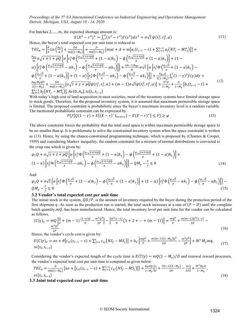
For batches 2, … ,𝑚𝑚, the expected shortage amount is: 𝐸𝐸(𝑋𝑋2 − 𝑟𝑟2)+ = ∫ (𝑥𝑥2 − 𝑟𝑟2)𝑓𝑓(𝑥𝑥2)𝑑𝑑𝑥𝑥2 = 𝜎𝜎√𝑡𝑡
∞𝑝𝑝2 𝜓𝜓(𝑟𝑟12, 𝑟𝑟22,𝛼𝛼) (11)
Hence, the buyer’s total expected cost per unit time is reduced to 𝑇𝑇𝐸𝐸𝐶𝐶𝑏𝑏 = �𝜃𝜃
𝛿𝛿𝐿𝐿𝑙𝑙 �𝐴𝐴0
𝐴𝐴� + 𝐷𝐷𝐴𝐴
𝑚𝑚𝑄𝑄�1−𝑀𝑀𝛾𝛾�� + 𝐷𝐷
𝑚𝑚𝑄𝑄�1−𝑀𝑀𝛾𝛾��𝑚𝑚𝑚𝑚𝑡𝑡 + 𝐴𝐴 + 𝑚𝑚�𝑎𝑎𝑖𝑖(𝑡𝑡𝑖𝑖−1 − 𝑡𝑡) + ∑ 𝑎𝑎𝑗𝑗�𝑁𝑁𝑇𝑇𝑗𝑗 − 𝑀𝑀𝑇𝑇𝑗𝑗�𝑖𝑖−1
𝑗𝑗=1 �� +ℎ𝑏𝑏1𝑚𝑚𝜎𝜎�𝑠𝑠 + 𝑡𝑡 + 𝑝𝑝𝑄𝑄 �𝛼𝛼 �𝑟𝑟11Φ �𝜇𝜇∗�𝑡𝑡+𝑠𝑠+𝑝𝑝𝑄𝑄
𝜎𝜎+ (1 − 𝛼𝛼)𝑘𝑘1� − 𝜙𝜙 �𝜇𝜇∗�𝑡𝑡+𝑠𝑠+𝑝𝑝𝑄𝑄
𝜎𝜎+ (1 − 𝛼𝛼)𝑘𝑘1�� + (1 −
𝛼𝛼) �𝑟𝑟21Φ �𝜇𝜇∗�𝑡𝑡+𝑠𝑠+𝑝𝑝𝑄𝑄𝜎𝜎
− 𝛼𝛼𝑘𝑘1� − 𝜙𝜙 �𝜇𝜇∗�𝑡𝑡+𝑠𝑠+𝑝𝑝𝑄𝑄𝜎𝜎
− 𝛼𝛼𝑘𝑘1��� + (𝑚𝑚−1)ℎ𝑏𝑏1𝑚𝑚
𝜎𝜎√𝑡𝑡 �𝛼𝛼 �𝑟𝑟11Φ �𝜇𝜇∗√𝑡𝑡𝜎𝜎
+ (1 − 𝛼𝛼)𝑘𝑘1� −
𝜙𝜙 �𝜇𝜇∗√𝑡𝑡𝜎𝜎
+ (1 − 𝛼𝛼)𝑘𝑘1�� + (1 − 𝛼𝛼) �𝑟𝑟21Φ �𝜇𝜇∗√𝑡𝑡𝜎𝜎− 𝛼𝛼𝑘𝑘1� − 𝜙𝜙 �𝜇𝜇∗√𝑡𝑡
𝜎𝜎− 𝛼𝛼𝑘𝑘1��� + ℎ𝑏𝑏1𝑄𝑄
2�1−𝑀𝑀𝛾𝛾�∫ (1 − 𝛾𝛾)2𝑓𝑓(𝛾𝛾)𝑑𝑑𝛾𝛾10 +
ℎ𝑏𝑏2𝑀𝑀𝛾𝛾𝑄𝑄𝐷𝐷𝜆𝜆�1−𝑀𝑀𝛾𝛾�
+ 𝐷𝐷𝐷𝐷𝑚𝑚𝑄𝑄�1−𝑀𝑀𝛾𝛾�
�𝜎𝜎�𝑡𝑡 + 𝑠𝑠 + 𝑝𝑝𝑄𝑄𝜓𝜓(𝑟𝑟11 , 𝑟𝑟21,𝛼𝛼) + (𝑚𝑚 − 1)𝜎𝜎√𝑡𝑡𝜓𝜓(𝑟𝑟12, 𝑟𝑟22,𝛼𝛼)� + 𝑆𝑆𝑐𝑐𝐷𝐷1−𝑀𝑀𝛾𝛾
+ 𝐷𝐷1−𝑀𝑀𝛾𝛾
�𝑏𝑏𝑖𝑖(𝑡𝑡𝑖𝑖−1 − 𝑡𝑡) +
∑ 𝑏𝑏𝑗𝑗�𝑁𝑁𝑇𝑇𝑗𝑗 − 𝑀𝑀𝑇𝑇𝑗𝑗�𝑖𝑖−1𝑗𝑗=1 �,𝐴𝐴𝛾𝛾(0,𝐴𝐴0], 𝑡𝑡𝛾𝛾[𝑡𝑡𝑖𝑖, 𝑡𝑡𝑖𝑖−1]
(12)
With today’s high cost of land acquisition in most societies, most of the inventory systems have limited storage space to stock goods. Therefore, for the proposed inventory system, it is assumed that maximum permissible storage space is limited. The proposed constraint is probabilistic since the buyer’s maximum inventory level is a random variable. The mentioned probabilistic constraint can be expressed by
𝑃𝑃{𝑓𝑓[𝑄𝑄(1 − 𝛾𝛾) + 𝐸𝐸[(𝑋𝑋 − 𝑟𝑟)−𝐼𝐼0<𝑋𝑋<𝑝𝑝] − 𝐸𝐸(𝑋𝑋 − 𝑟𝑟)+] ≤ 𝐹𝐹} ≥ 𝜑𝜑 (13)
The above constraint forces the probability that the total used space is within maximum permissible storage space to be no smaller than 𝜑𝜑. It is problematic to solve the constrained inventory system when the space constraint is written as (13). Hence, by using the chance-constrained programming technique, which is proposed by (Charnes & Cooper, 1959) and considering Markov inequality, the random constraint for a mixture of normal distributions is converted to the crisp one which is given by:
𝜑𝜑1𝑄𝑄 + 𝜎𝜎�𝑠𝑠 + 𝑡𝑡 + 𝑝𝑝𝑄𝑄 �𝛼𝛼 �𝑟𝑟11Φ �𝜇𝜇∗�𝑠𝑠+𝑡𝑡+𝑝𝑝𝑄𝑄𝜎𝜎
+ (1 − 𝛼𝛼)𝑘𝑘1� − 𝜙𝜙 �𝜇𝜇∗�𝑠𝑠+𝑡𝑡+𝑝𝑝𝑄𝑄𝜎𝜎
+ (1 − 𝛼𝛼)𝑘𝑘1�� +
(1 − 𝛼𝛼) �𝑟𝑟21Φ �𝜇𝜇∗�𝑠𝑠+𝑡𝑡+𝑝𝑝𝑄𝑄𝜎𝜎
− 𝛼𝛼𝑘𝑘1� − 𝜙𝜙 �𝜇𝜇∗�𝑠𝑠+𝑡𝑡+𝑝𝑝𝑄𝑄𝜎𝜎
− 𝛼𝛼𝑘𝑘1��� − 𝑄𝑄𝑀𝑀𝛾𝛾 −𝐹𝐹𝑓𝑓≤ 0
(14)
And 𝜑𝜑2𝑄𝑄 + 𝜎𝜎√𝑡𝑡 �𝛼𝛼 �𝑟𝑟12Φ �𝜇𝜇∗√𝑡𝑡
𝜎𝜎+ (1 − 𝛼𝛼)𝑘𝑘1� − 𝜙𝜙 �𝜇𝜇∗√𝑡𝑡
𝜎𝜎+ (1 − 𝛼𝛼)𝑘𝑘1�� + (1 − 𝛼𝛼) �𝑟𝑟22Φ �𝜇𝜇∗√𝑡𝑡
𝜎𝜎− 𝛼𝛼𝑘𝑘1� − 𝜙𝜙 �𝜇𝜇∗√𝑡𝑡
𝜎𝜎− 𝛼𝛼𝑘𝑘1��� −
𝑄𝑄𝑀𝑀𝛾𝛾 −𝐹𝐹𝑓𝑓≤ 0 (15)
3.2 Vendor’s total expected cost per unit time The initial stock in the system, 𝑄𝑄𝐷𝐷 𝑃𝑃⁄ , is the amount of inventory required by the buyer during the protection period of the first shipment 𝑞𝑞. As soon as the production run is started, the total stock increases at a rate of (𝑃𝑃 − 𝐷𝐷) until the complete batch quantity,𝑚𝑚𝑄𝑄, has been manufactured. Hence, the total inventory level per unit time for the vendor can be calculated as follows.
(𝐶𝐶|𝛾𝛾)𝑣𝑣 = 𝑚𝑚𝑄𝑄 �𝑄𝑄𝑃𝑃
+ (𝑚𝑚 − 1) (1−𝛾𝛾)𝑄𝑄𝐷𝐷
− 𝑚𝑚2𝑄𝑄2
2𝑃𝑃� − �𝑄𝑄
2(1−𝛾𝛾)𝐷𝐷
�1 + 2 + ⋯+ (𝑚𝑚 − 1)�� = 𝑚𝑚𝑄𝑄2
𝑃𝑃+ 𝑚𝑚(𝑚𝑚−1)𝑄𝑄2(1−𝛾𝛾)
2𝐷𝐷−
𝑚𝑚2𝑄𝑄2
2𝑃𝑃
(16)
Hence, the vendor’s cycle cost is given by: 𝐸𝐸(𝐶𝐶|𝛾𝛾)𝑣𝑣 = 𝑎𝑎𝑠𝑠 + 𝜃𝜃�𝑐𝑐𝑠𝑠𝑖𝑖(𝑠𝑠𝑖𝑖−1 − 𝑠𝑠) + ∑ 𝑐𝑐𝑠𝑠𝑗𝑗�𝑁𝑁𝑆𝑆𝑗𝑗 − 𝑀𝑀𝑆𝑆𝑗𝑗�𝑖𝑖
𝑗𝑗=1 � + ℎ𝑉𝑉 �𝑚𝑚𝑄𝑄2
𝑃𝑃+ 𝑚𝑚(𝑚𝑚−1)�1−𝑀𝑀𝛾𝛾�𝑄𝑄2
2𝐷𝐷− 𝑚𝑚2𝑄𝑄2
2𝑃𝑃� + 𝑊𝑊𝑐𝑐𝑀𝑀𝛾𝛾𝑚𝑚𝑞𝑞,
𝑠𝑠𝛾𝛾[𝑠𝑠𝑖𝑖 , 𝑠𝑠𝑖𝑖−1]
(17)
Considering the vendor’s expected length of the cycle time is 𝐸𝐸(𝑇𝑇|𝛾𝛾) = 𝑚𝑚𝑄𝑄(1 −𝑀𝑀𝛾𝛾) 𝐷𝐷⁄ and renewal reward processes, the vendor’s expected total cost per unit time is computed as given below 𝑇𝑇𝐸𝐸𝐶𝐶𝑣𝑣 = 𝐷𝐷
𝑚𝑚𝑄𝑄�1−𝑀𝑀𝛾𝛾��𝑎𝑎𝑠𝑠 + �𝑐𝑐𝑠𝑠𝑖𝑖(𝑠𝑠𝑖𝑖−1 − 𝑠𝑠) + ∑ 𝑐𝑐𝑠𝑠𝑗𝑗�𝑁𝑁𝑆𝑆𝑗𝑗 − 𝑀𝑀𝑆𝑆𝑗𝑗�𝑖𝑖−1
𝑗𝑗=1 �� + ℎ𝑉𝑉𝐷𝐷𝑄𝑄1−𝑀𝑀𝛾𝛾
�1𝑃𝑃
+(𝑚𝑚−1)�1−𝑀𝑀𝛾𝛾�
2𝐷𝐷− 𝑚𝑚
2𝑃𝑃� + 𝑊𝑊𝑐𝑐𝑀𝑀𝛾𝛾𝐷𝐷
1−𝑀𝑀𝛾𝛾,
𝑠𝑠𝛾𝛾[𝑠𝑠𝑖𝑖 , 𝑠𝑠𝑖𝑖−1]
(18)
3.3 Joint total expected cost per unit time
1324

Proceedings of the 5th NA International Conference on Industrial Engineering and Operations Management Detroit, Michigan, USA, August 10 - 14, 2020
© IEOM Society International
Once the buyer and vendor have built up a long-term strategic partnership, they can jointly determine the best policy for both parties. Accordingly, the joint total expected cost per unit time can be obtained as the sum of the buyer’s and the vendor’s total expected costs per unit time. That is, 𝐽𝐽𝐸𝐸𝐴𝐴𝐶𝐶(𝑄𝑄,𝐴𝐴, 𝑟𝑟1, 𝑟𝑟2, 𝑠𝑠 , 𝑡𝑡,𝑚𝑚) = �𝜃𝜃
𝛿𝛿𝐿𝐿𝑙𝑙 �𝐴𝐴0
𝐴𝐴� + 𝐷𝐷𝐴𝐴
𝑚𝑚𝑄𝑄�1−𝑀𝑀𝛾𝛾�� + ℎ𝑏𝑏1
𝑚𝑚𝜎𝜎�𝑠𝑠 + 𝑡𝑡 + 𝑝𝑝𝑄𝑄 �𝛼𝛼 �𝑟𝑟11Φ�𝜇𝜇∗�𝑡𝑡+𝑠𝑠+𝑝𝑝𝑄𝑄
𝜎𝜎+ (1 − 𝛼𝛼)𝑘𝑘1� − 𝜙𝜙 �𝜇𝜇∗�𝑡𝑡+𝑠𝑠+𝑝𝑝𝑄𝑄
𝜎𝜎+
(1 − 𝛼𝛼)𝑘𝑘1�� + (1 − 𝛼𝛼) �𝑟𝑟21Φ�𝜇𝜇∗�𝑡𝑡+𝑠𝑠+𝑝𝑝𝑄𝑄𝜎𝜎
− 𝛼𝛼𝑘𝑘1� − 𝜙𝜙 �𝜇𝜇∗�𝑡𝑡+𝑠𝑠+𝑝𝑝𝑄𝑄𝜎𝜎
− 𝛼𝛼𝑘𝑘1��� + (𝑚𝑚−1)ℎ𝑏𝑏1𝑚𝑚
𝜎𝜎√𝑡𝑡 �𝛼𝛼 �𝑟𝑟12Φ �𝜇𝜇∗√𝑡𝑡𝜎𝜎
+ (1 − 𝛼𝛼)𝑘𝑘1� −
𝜙𝜙 �𝜇𝜇∗√𝑡𝑡𝜎𝜎
+ (1 − 𝛼𝛼)𝑘𝑘1�� + (1 − 𝛼𝛼) �𝑟𝑟22Φ�𝜇𝜇∗√𝑡𝑡𝜎𝜎
− 𝛼𝛼𝑘𝑘1� − 𝜙𝜙 �𝜇𝜇∗√𝑡𝑡𝜎𝜎
− 𝛼𝛼𝑘𝑘1��� + ℎ𝑏𝑏1𝑄𝑄2�1−𝑀𝑀𝛾𝛾�
∫ (1 − 𝛾𝛾)2𝑓𝑓(𝛾𝛾)𝑑𝑑𝛾𝛾10 + ℎ𝑏𝑏2𝑀𝑀𝛾𝛾𝑄𝑄𝐷𝐷
𝜆𝜆�1−𝑀𝑀𝛾𝛾�+
𝐷𝐷𝐷𝐷𝑚𝑚𝑄𝑄�1−𝑀𝑀𝛾𝛾�
�𝜎𝜎�𝑡𝑡 + 𝑠𝑠 + 𝑝𝑝𝑄𝑄𝜓𝜓(𝑟𝑟11, 𝑟𝑟21,𝛼𝛼) + (𝑚𝑚 − 1)𝜎𝜎√𝑡𝑡𝜓𝜓(𝑟𝑟12, 𝑟𝑟22,𝛼𝛼)� + 𝑆𝑆𝑐𝑐𝐷𝐷1−𝑀𝑀𝛾𝛾
+ 𝑊𝑊𝑐𝑐𝑀𝑀𝛾𝛾𝐷𝐷1−𝑀𝑀𝛾𝛾
+ 𝐷𝐷𝑚𝑚𝑄𝑄�1−𝑀𝑀𝛾𝛾�
�𝑚𝑚𝑚𝑚𝑡𝑡 + 𝐴𝐴 + 𝑎𝑎𝑠𝑠 + �𝑐𝑐𝑠𝑠𝑖𝑖(𝑠𝑠𝑖𝑖−1 −
𝑠𝑠) + ∑ 𝑐𝑐𝑠𝑠𝑗𝑗�𝑁𝑁𝑆𝑆𝑗𝑗 − 𝑀𝑀𝑆𝑆𝑗𝑗�𝑖𝑖−1𝑗𝑗=1 � + 𝑚𝑚�𝑎𝑎𝑖𝑖(𝑡𝑡𝑖𝑖−1 − 𝑡𝑡) + ∑ 𝑎𝑎𝑗𝑗�𝑁𝑁𝑇𝑇𝑗𝑗 − 𝑀𝑀𝑇𝑇𝑗𝑗�𝑖𝑖−1
𝑗𝑗=1 �� + 𝐷𝐷1−𝑀𝑀𝛾𝛾
�𝑏𝑏𝑖𝑖(𝑡𝑡𝑖𝑖−1 − 𝑡𝑡) + ∑ 𝑏𝑏𝑗𝑗�𝑁𝑁𝑇𝑇𝑗𝑗 − 𝑀𝑀𝑇𝑇𝑗𝑗�𝑖𝑖−1𝑗𝑗=1 � +
ℎ𝑣𝑣𝐷𝐷𝑄𝑄1−𝑀𝑀𝛾𝛾
�1𝑃𝑃
+(𝑚𝑚−1)�1−𝑀𝑀𝛾𝛾�
2𝐷𝐷− 𝑚𝑚
2𝑃𝑃�
Subject to: 𝜎𝜎�𝑠𝑠 + 𝑡𝑡 + 𝑝𝑝𝑄𝑄[𝑟𝑟11 + 𝑘𝑘1(1 − 𝛼𝛼)] − 𝜎𝜎√𝑡𝑡[𝑟𝑟12 + 𝑘𝑘1(1 − 𝛼𝛼)] = 0 𝛾𝛾𝑄𝑄 + 𝜎𝜎�𝑠𝑠 + 𝑡𝑡 + 𝑝𝑝𝑄𝑄 �𝛼𝛼 �𝑟𝑟11Φ�𝜇𝜇∗�𝑡𝑡+𝑠𝑠+𝑝𝑝𝑄𝑄
𝜎𝜎+ (1 − 𝛼𝛼)𝑘𝑘1� − 𝜙𝜙 �𝜇𝜇∗�𝑡𝑡+𝑠𝑠+𝑝𝑝𝑄𝑄
𝜎𝜎+ (1 − 𝛼𝛼)𝑘𝑘1�� + (1 − 𝛼𝛼) �𝑟𝑟21Φ �𝜇𝜇∗�𝑡𝑡+𝑠𝑠+𝑝𝑝𝑄𝑄
𝜎𝜎− 𝛼𝛼𝑘𝑘1� −
𝜙𝜙 �𝜇𝜇∗�𝑡𝑡+𝑠𝑠+𝑝𝑝𝑄𝑄𝜎𝜎
− 𝛼𝛼𝑘𝑘1��� − 𝑄𝑄𝑀𝑀𝛾𝛾 −𝐹𝐹𝑓𝑓≤ 0
𝛾𝛾𝑄𝑄 + 𝜎𝜎√𝑡𝑡 �𝛼𝛼 �𝑟𝑟12Φ �𝜇𝜇∗√𝑡𝑡
𝜎𝜎+ (1 − 𝛼𝛼)𝑘𝑘1� − 𝜙𝜙 �𝜇𝜇∗√𝑡𝑡
𝜎𝜎+ (1 − 𝛼𝛼)𝑘𝑘1�� + (1 − 𝛼𝛼) �𝑟𝑟22Φ�𝜇𝜇∗√𝑡𝑡
𝜎𝜎− 𝛼𝛼𝑘𝑘1� − 𝜙𝜙 �𝜇𝜇∗√𝑡𝑡
𝜎𝜎− 𝛼𝛼𝑘𝑘1��� − 𝑄𝑄𝑀𝑀𝛾𝛾 −
𝐹𝐹𝑓𝑓≤ 0
Over 𝑄𝑄, 𝑟𝑟1, 𝑟𝑟2 ≥ 0,𝐴𝐴𝛾𝛾(0,𝐴𝐴0], 𝑡𝑡𝛾𝛾[𝑡𝑡𝑖𝑖 , 𝑡𝑡𝑖𝑖−1], 𝑠𝑠𝛾𝛾[𝑠𝑠𝑖𝑖 , 𝑠𝑠𝑖𝑖−1],𝑚𝑚 > 0 𝑖𝑖𝑙𝑙𝑡𝑡𝑒𝑒𝑔𝑔𝑒𝑒𝑟𝑟 (19) The above model (19) can be solved with the Lagrange multiplier method as given below: 𝐽𝐽𝐸𝐸𝐴𝐴𝐶𝐶(𝑄𝑄,𝐴𝐴, 𝑟𝑟1, 𝑟𝑟2, 𝑠𝑠 , 𝑡𝑡,𝑚𝑚, 𝜆𝜆1, 𝜆𝜆2, 𝜆𝜆3) = �𝜃𝜃
𝛿𝛿𝐿𝐿𝑙𝑙 �𝐴𝐴0
𝐴𝐴� + 𝐷𝐷𝐴𝐴
𝑚𝑚𝑄𝑄�1−𝑀𝑀𝛾𝛾�� + ℎ𝑏𝑏1
𝑚𝑚𝜎𝜎�𝑠𝑠 + 𝑡𝑡 + 𝑝𝑝𝑄𝑄 �𝛼𝛼 �𝑟𝑟11Φ�𝜇𝜇∗�𝑡𝑡+𝑠𝑠+𝑝𝑝𝑄𝑄
𝜎𝜎+ (1 − 𝛼𝛼)𝑘𝑘1� −
𝜙𝜙 �𝜇𝜇∗�𝑡𝑡+𝑠𝑠+𝑝𝑝𝑄𝑄𝜎𝜎
+ (1 − 𝛼𝛼)𝑘𝑘1�� + (1 − 𝛼𝛼) �𝑟𝑟21Φ�𝜇𝜇∗�𝑡𝑡+𝑠𝑠+𝑝𝑝𝑄𝑄𝜎𝜎
− 𝛼𝛼𝑘𝑘1� − 𝜙𝜙 �𝜇𝜇∗�𝑡𝑡+𝑠𝑠+𝑝𝑝𝑄𝑄𝜎𝜎
− 𝛼𝛼𝑘𝑘1��� + (𝑚𝑚−1)ℎ𝑏𝑏1𝑚𝑚
𝜎𝜎√𝑡𝑡 �𝛼𝛼 �𝑟𝑟12Φ�𝜇𝜇∗√𝑡𝑡𝜎𝜎
+
(1 − 𝛼𝛼)𝑘𝑘1� − 𝜙𝜙 �𝜇𝜇∗√𝑡𝑡𝜎𝜎
+ (1 − 𝛼𝛼)𝑘𝑘1�� + (1 − 𝛼𝛼) �𝑟𝑟22Φ�𝜇𝜇∗√𝑡𝑡𝜎𝜎
− 𝛼𝛼𝑘𝑘1� − 𝜙𝜙 �𝜇𝜇∗√𝑡𝑡𝜎𝜎
− 𝛼𝛼𝑘𝑘1��� + ℎ𝑏𝑏1𝑄𝑄2�1−𝑀𝑀𝛾𝛾�
∫ (1 − 𝛾𝛾)2𝑓𝑓(𝛾𝛾)𝑑𝑑𝛾𝛾10 + ℎ𝑏𝑏2𝑀𝑀𝛾𝛾𝑄𝑄𝐷𝐷
𝜆𝜆�1−𝑀𝑀𝛾𝛾�+
𝐷𝐷𝐷𝐷𝑚𝑚𝑄𝑄�1−𝑀𝑀𝛾𝛾�
�𝜎𝜎�𝑡𝑡 + 𝑠𝑠 + 𝑝𝑝𝑄𝑄𝜓𝜓(𝑟𝑟11, 𝑟𝑟21,𝛼𝛼) + (𝑚𝑚 − 1)𝜎𝜎√𝑡𝑡𝜓𝜓(𝑟𝑟12, 𝑟𝑟22,𝛼𝛼)� + 𝑆𝑆𝑐𝑐𝐷𝐷1−𝑀𝑀𝛾𝛾
+ 𝑊𝑊𝑐𝑐𝑀𝑀𝛾𝛾𝐷𝐷1−𝑀𝑀𝛾𝛾
+ 𝐷𝐷𝑚𝑚𝑄𝑄�1−𝑀𝑀𝛾𝛾�
�𝑚𝑚𝑚𝑚𝑡𝑡 + 𝑎𝑎𝑠𝑠 +
�𝑐𝑐𝑠𝑠𝑖𝑖(𝑠𝑠𝑖𝑖−1 − 𝑠𝑠) + ∑ 𝑐𝑐𝑠𝑠𝑗𝑗�𝑁𝑁𝑆𝑆𝑗𝑗 −𝑀𝑀𝑆𝑆𝑗𝑗�𝑖𝑖−1𝑗𝑗=1 � + 𝑚𝑚�𝑎𝑎𝑖𝑖(𝑡𝑡𝑖𝑖−1 − 𝑡𝑡) + ∑ 𝑎𝑎𝑗𝑗�𝑁𝑁𝑇𝑇𝑗𝑗 − 𝑀𝑀𝑇𝑇𝑗𝑗�𝑖𝑖−1
𝑗𝑗=1 �� + 𝐷𝐷�1−𝑀𝑀𝛾𝛾�
�𝑏𝑏𝑖𝑖(𝑡𝑡𝑖𝑖−1 − 𝑡𝑡) +
∑ 𝑏𝑏𝑗𝑗�𝑁𝑁𝑇𝑇𝑗𝑗 − 𝑀𝑀𝑇𝑇𝑗𝑗�𝑖𝑖−1𝑗𝑗=1 � + ℎ𝑣𝑣𝐷𝐷𝑄𝑄
1−𝑀𝑀𝛾𝛾�1𝑃𝑃
+(𝑚𝑚−1)�1−𝑀𝑀𝛾𝛾�
2𝐷𝐷− 𝑚𝑚
2𝑃𝑃� + 𝜆𝜆1𝜎𝜎�𝑠𝑠 + 𝑡𝑡 + 𝑝𝑝𝑄𝑄[𝑟𝑟11 + 𝑘𝑘1(1 − 𝛼𝛼)] − 𝜆𝜆1𝜎𝜎√𝑡𝑡[𝑟𝑟12 + 𝑘𝑘1(1 − 𝛼𝛼)] +
𝜆𝜆2𝜎𝜎�𝑠𝑠 + 𝑡𝑡 + 𝑝𝑝𝑄𝑄 �𝛼𝛼 �𝑟𝑟11Φ�𝜇𝜇∗�𝑡𝑡+𝑠𝑠+𝑝𝑝𝑄𝑄𝜎𝜎
+ (1 − 𝛼𝛼)𝑘𝑘1� − 𝜙𝜙 �𝜇𝜇∗�𝑡𝑡+𝑠𝑠+𝑝𝑝𝑄𝑄𝜎𝜎
+ (1 − 𝛼𝛼)𝑘𝑘1�� + (1 − 𝛼𝛼) �𝑟𝑟21Φ�𝜇𝜇∗�𝑡𝑡+𝑠𝑠+𝑝𝑝𝑄𝑄𝜎𝜎
− 𝛼𝛼𝑘𝑘1� −
𝜙𝜙 �𝜇𝜇∗�𝑡𝑡+𝑠𝑠+𝑝𝑝𝑄𝑄𝜎𝜎
− 𝛼𝛼𝑘𝑘1��� + 𝜆𝜆2𝑄𝑄�𝜑𝜑1 − 𝑀𝑀𝛾𝛾� − 𝜆𝜆2𝐹𝐹𝑓𝑓
+ 𝜆𝜆3𝜎𝜎√𝑡𝑡 �𝛼𝛼 �𝑟𝑟12Φ�𝜇𝜇∗√𝑡𝑡𝜎𝜎
+ (1 − 𝛼𝛼)𝑘𝑘1� − 𝜙𝜙 �𝜇𝜇∗√𝑡𝑡𝜎𝜎
+ (1 − 𝛼𝛼)𝑘𝑘1�� +
(1 − 𝛼𝛼) �𝑟𝑟22Φ�𝜇𝜇∗√𝑡𝑡𝜎𝜎
− 𝛼𝛼𝑘𝑘1� − 𝜙𝜙 �𝜇𝜇∗√𝑡𝑡𝜎𝜎
− 𝛼𝛼𝑘𝑘1��� + 𝜆𝜆3𝑄𝑄�𝜑𝜑2 −𝑀𝑀𝛾𝛾� − 𝜆𝜆3𝐹𝐹𝑓𝑓
(20)
Where 𝜆𝜆1 is free in sign and 𝜆𝜆2 and 𝜆𝜆3 are nonnegative variables. To solve the above nonlinear programming problem, this study temporarily ignores the constraint 0 ≤ 𝐴𝐴 ≤ 𝐴𝐴0 and relaxes the integer requirement on 𝑚𝑚(the number of shipments from the vendor to the buyer during a cycle). It can be shown that for fixed 𝑄𝑄,𝐴𝐴, 𝑟𝑟1, 𝑟𝑟2, 𝑠𝑠 , 𝑡𝑡,𝑚𝑚, 𝜆𝜆1, 𝜆𝜆2 , the optimal setup and transportation time occur at the end of points of interval 𝑠𝑠𝛾𝛾[𝑠𝑠𝑖𝑖 , 𝑠𝑠𝑖𝑖−1] and 𝑡𝑡𝛾𝛾[𝑡𝑡𝑖𝑖 , 𝑡𝑡𝑖𝑖−1] respectively (Chang et al., 2006). This result simplifies the search for the optimal solution to this inventory problem considerably. Therefore, the Kuhn-Tucker necessary conditions for minimization of the function (20) are as follows: 𝜕𝜕𝜕𝜕𝜕𝜕𝐴𝐴𝜕𝜕𝜕𝜕𝑄𝑄
= 0, 𝜕𝜕𝜕𝜕𝜕𝜕𝐴𝐴𝜕𝜕𝜕𝜕𝑝𝑝1
= 0, 𝜕𝜕𝜕𝜕𝜕𝜕𝐴𝐴𝜕𝜕𝜕𝜕𝑝𝑝2
= 0, 𝜕𝜕𝜕𝜕𝜕𝜕𝐴𝐴𝜕𝜕𝜕𝜕𝐴𝐴
= 0 (21) 𝜎𝜎�𝑠𝑠 + 𝑡𝑡 + 𝑝𝑝𝑄𝑄[𝑟𝑟11 + 𝑘𝑘1(1 − 𝛼𝛼)] − 𝜎𝜎√𝑡𝑡[𝑟𝑟12 + 𝑘𝑘1(1 − 𝛼𝛼)] = 0 (22)
𝜆𝜆2 �𝜑𝜑1𝑄𝑄 + 𝜎𝜎�𝑠𝑠 + 𝑡𝑡 + 𝑝𝑝𝑄𝑄 �𝛼𝛼 �𝑟𝑟11Φ�𝜇𝜇∗�𝑡𝑡+𝑠𝑠+𝑝𝑝𝑄𝑄𝜎𝜎
+ (1 − 𝛼𝛼)𝑘𝑘1� − 𝜙𝜙 �𝜇𝜇∗�𝑡𝑡+𝑠𝑠+𝑝𝑝𝑄𝑄𝜎𝜎
+ (1 − 𝛼𝛼)𝑘𝑘1�� + (1 − 𝛼𝛼) �𝑟𝑟21Φ �𝜇𝜇∗�𝑡𝑡+𝑠𝑠+𝑝𝑝𝑄𝑄𝜎𝜎
− 𝛼𝛼𝑘𝑘1� −
𝜙𝜙 �𝜇𝜇∗�𝑡𝑡+𝑠𝑠+𝑝𝑝𝑄𝑄𝜎𝜎
− 𝛼𝛼𝑘𝑘1��� − 𝑄𝑄𝑀𝑀𝛾𝛾 −𝐹𝐹𝑓𝑓� = 0 (23)
1325
Proceedings of the 5th NA International Conference on Industrial Engineering and Operations Management Detroit, Michigan, USA, August 10 - 14, 2020
© IEOM Society International
𝜆𝜆3 �𝛾𝛾𝑄𝑄 + 𝜎𝜎√𝑡𝑡 �𝛼𝛼 �𝑟𝑟12Φ�𝜇𝜇∗√𝑡𝑡𝜎𝜎
+ (1 − 𝛼𝛼)𝑘𝑘1� − 𝜙𝜙 �𝜇𝜇∗√𝑡𝑡𝜎𝜎
+ (1 − 𝛼𝛼)𝑘𝑘1��+ (1 − 𝛼𝛼) �𝑟𝑟22Φ�𝜇𝜇∗√𝑡𝑡𝜎𝜎
− 𝛼𝛼𝑘𝑘1� − 𝜙𝜙 �𝜇𝜇∗√𝑡𝑡𝜎𝜎
− 𝛼𝛼𝑘𝑘1��� − 𝑄𝑄𝑀𝑀𝛾𝛾 −𝐹𝐹𝑓𝑓� = 0
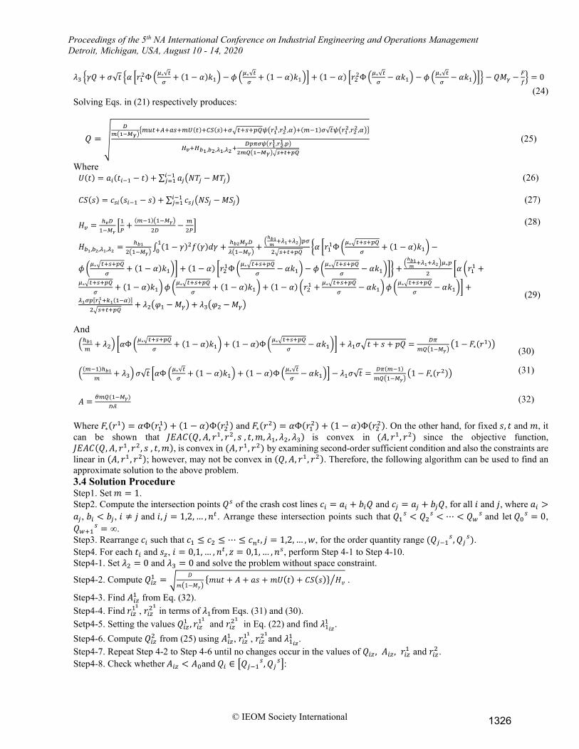
(24) Solving Eqs. in (21) respectively produces:
𝑄𝑄 = �𝐷𝐷
𝑚𝑚�1−𝑀𝑀𝛾𝛾��𝑚𝑚𝑝𝑝𝑡𝑡+𝐴𝐴+𝑎𝑎𝑠𝑠+𝑚𝑚𝑚𝑚(𝑡𝑡)+𝜕𝜕𝑆𝑆(𝑠𝑠)+𝜎𝜎�𝑡𝑡+𝑠𝑠+𝑝𝑝𝑄𝑄𝜓𝜓�𝑝𝑝11,𝑝𝑝21,𝛼𝛼�+(𝑚𝑚−1)𝜎𝜎√𝑡𝑡𝜓𝜓�𝑝𝑝12,𝑝𝑝22,𝛼𝛼��
𝐻𝐻𝑣𝑣+𝐻𝐻𝑏𝑏1,𝑏𝑏2,𝜆𝜆1,𝜆𝜆2+𝐷𝐷𝐷𝐷𝐷𝐷𝐷𝐷𝐷𝐷�𝑟𝑟1
1,𝑟𝑟21,𝐷𝐷�
2𝑚𝑚𝑚𝑚�1−𝑀𝑀𝛾𝛾��𝑠𝑠+𝑡𝑡+𝐷𝐷𝑚𝑚
(25)
Where 𝑈𝑈(𝑡𝑡) = 𝑎𝑎𝑖𝑖(𝑡𝑡𝑖𝑖−1 − 𝑡𝑡) + ∑ 𝑎𝑎𝑗𝑗�𝑁𝑁𝑇𝑇𝑗𝑗 −𝑀𝑀𝑇𝑇𝑗𝑗�𝑖𝑖−1
𝑗𝑗=1
(26)
𝐶𝐶𝑆𝑆(𝑠𝑠) = 𝑐𝑐𝑠𝑠𝑖𝑖(𝑠𝑠𝑖𝑖−1 − 𝑠𝑠) + ∑ 𝑐𝑐𝑠𝑠𝑗𝑗�𝑁𝑁𝑆𝑆𝑗𝑗 − 𝑀𝑀𝑆𝑆𝑗𝑗�𝑖𝑖−1𝑗𝑗=1
(27)
𝐻𝐻𝑣𝑣 = ℎ𝑣𝑣𝐷𝐷1−𝑀𝑀𝛾𝛾
�1𝑃𝑃
+(𝑚𝑚−1)�1−𝑀𝑀𝛾𝛾�
2𝐷𝐷− 𝑚𝑚
2𝑃𝑃� (28)
𝐻𝐻𝑏𝑏1,𝑏𝑏2,𝜆𝜆1,𝜆𝜆2 = ℎ𝑏𝑏12�1−𝑀𝑀𝛾𝛾�
∫ (1 − 𝛾𝛾)2𝑓𝑓(𝛾𝛾)𝑑𝑑𝛾𝛾10 + ℎ𝑏𝑏2𝑀𝑀𝛾𝛾𝐷𝐷
𝜆𝜆�1−𝑀𝑀𝛾𝛾�+
�ℎ𝑏𝑏1𝑚𝑚 +𝜆𝜆1+𝜆𝜆2�𝑝𝑝𝜎𝜎
2�𝑠𝑠+𝑡𝑡+𝑝𝑝𝑄𝑄�𝛼𝛼 �𝑟𝑟11Φ�𝜇𝜇∗�𝑡𝑡+𝑠𝑠+𝑝𝑝𝑄𝑄
𝜎𝜎+ (1 − 𝛼𝛼)𝑘𝑘1� −
𝜙𝜙 �𝜇𝜇∗�𝑡𝑡+𝑠𝑠+𝑝𝑝𝑄𝑄𝜎𝜎
+ (1 − 𝛼𝛼)𝑘𝑘1�� + (1 − 𝛼𝛼) �𝑟𝑟21Φ�𝜇𝜇∗�𝑡𝑡+𝑠𝑠+𝑝𝑝𝑄𝑄𝜎𝜎
− 𝛼𝛼𝑘𝑘1� − 𝜙𝜙 �𝜇𝜇∗�𝑡𝑡+𝑠𝑠+𝑝𝑝𝑄𝑄𝜎𝜎
− 𝛼𝛼𝑘𝑘1��� +�ℎ𝑏𝑏1𝑚𝑚 +𝜆𝜆1+𝜆𝜆2�𝜇𝜇∗𝑝𝑝
2�𝛼𝛼 �𝑟𝑟11 +
𝜇𝜇∗�𝑡𝑡+𝑠𝑠+𝑝𝑝𝑄𝑄𝜎𝜎
+ (1 − 𝛼𝛼)𝑘𝑘1�𝜙𝜙 �𝜇𝜇∗�𝑡𝑡+𝑠𝑠+𝑝𝑝𝑄𝑄
𝜎𝜎+ (1 − 𝛼𝛼)𝑘𝑘1� + (1 − 𝛼𝛼) �𝑟𝑟21 + 𝜇𝜇∗�𝑡𝑡+𝑠𝑠+𝑝𝑝𝑄𝑄
𝜎𝜎− 𝛼𝛼𝑘𝑘1�𝜙𝜙 �
𝜇𝜇∗�𝑡𝑡+𝑠𝑠+𝑝𝑝𝑄𝑄𝜎𝜎
− 𝛼𝛼𝑘𝑘1�� +𝜆𝜆1𝜎𝜎𝑝𝑝[𝑝𝑝11+𝑘𝑘1(1−𝛼𝛼)]
2�𝑠𝑠+𝑡𝑡+𝑝𝑝𝑄𝑄+ 𝜆𝜆2�𝜑𝜑1 − 𝑀𝑀𝛾𝛾� + 𝜆𝜆3�𝜑𝜑2 −𝑀𝑀𝛾𝛾�
(29)
And �ℎ𝑏𝑏1𝑚𝑚
+ 𝜆𝜆2� �𝛼𝛼Φ �𝜇𝜇∗�𝑡𝑡+𝑠𝑠+𝑝𝑝𝑄𝑄𝜎𝜎
+ (1 − 𝛼𝛼)𝑘𝑘1� + (1 − 𝛼𝛼)Φ�𝜇𝜇∗�𝑡𝑡+𝑠𝑠+𝑝𝑝𝑄𝑄𝜎𝜎
− 𝛼𝛼𝑘𝑘1�� + 𝜆𝜆1𝜎𝜎�𝑡𝑡 + 𝑠𝑠 + 𝑝𝑝𝑄𝑄 = 𝐷𝐷𝐷𝐷𝑚𝑚𝑄𝑄�1−𝑀𝑀𝛾𝛾�
�1 − 𝐹𝐹∗(𝑟𝑟1)�
(30)
�(𝑚𝑚−1)ℎ𝑏𝑏1𝑚𝑚
+ 𝜆𝜆3� 𝜎𝜎√𝑡𝑡 �𝛼𝛼Φ �𝜇𝜇∗√𝑡𝑡𝜎𝜎
+ (1 − 𝛼𝛼)𝑘𝑘1� + (1 − 𝛼𝛼)Φ�𝜇𝜇∗√𝑡𝑡𝜎𝜎
− 𝛼𝛼𝑘𝑘1�� − 𝜆𝜆1𝜎𝜎√𝑡𝑡 = 𝐷𝐷𝐷𝐷(𝑚𝑚−1)𝑚𝑚𝑄𝑄�1−𝑀𝑀𝛾𝛾�
�1 − 𝐹𝐹∗(𝑟𝑟2)�
(31)
𝐴𝐴 = 𝜃𝜃𝑚𝑚𝑄𝑄(1−𝑀𝑀𝛾𝛾)𝐷𝐷𝛿𝛿
(32) Where 𝐹𝐹∗(𝑟𝑟1) = 𝛼𝛼Φ(𝑟𝑟11) + (1 − 𝛼𝛼)Φ(𝑟𝑟21) and 𝐹𝐹∗(𝑟𝑟2) = 𝛼𝛼Φ(𝑟𝑟12) + (1 − 𝛼𝛼)Φ(𝑟𝑟22). On the other hand, for fixed 𝑠𝑠, 𝑡𝑡 and 𝑚𝑚, it can be shown that 𝐽𝐽𝐸𝐸𝐴𝐴𝐶𝐶(𝑄𝑄,𝐴𝐴, 𝑟𝑟1, 𝑟𝑟2, 𝑠𝑠 , 𝑡𝑡,𝑚𝑚, 𝜆𝜆1, 𝜆𝜆2, 𝜆𝜆3) is convex in (𝐴𝐴, 𝑟𝑟1, 𝑟𝑟2) since the objective function, 𝐽𝐽𝐸𝐸𝐴𝐴𝐶𝐶(𝑄𝑄,𝐴𝐴, 𝑟𝑟1, 𝑟𝑟2, 𝑠𝑠 , 𝑡𝑡,𝑚𝑚), is convex in (𝐴𝐴, 𝑟𝑟1, 𝑟𝑟2) by examining second-order sufficient condition and also the constraints are linear in (𝐴𝐴, 𝑟𝑟1 , 𝑟𝑟2); however, may not be convex in (𝑄𝑄,𝐴𝐴, 𝑟𝑟1, 𝑟𝑟2). Therefore, the following algorithm can be used to find an approximate solution to the above problem. 3.4 Solution Procedure Step1. Set 𝑚𝑚 = 1. Step2. Compute the intersection points 𝑄𝑄𝑠𝑠 of the crash cost lines 𝑐𝑐𝑖𝑖 = 𝑎𝑎𝑖𝑖 + 𝑏𝑏𝑖𝑖𝑄𝑄 and 𝑐𝑐𝑗𝑗 = 𝑎𝑎𝑗𝑗 + 𝑏𝑏𝑗𝑗𝑄𝑄, for all 𝑖𝑖 and 𝑗𝑗, where 𝑎𝑎𝑖𝑖 >𝑎𝑎𝑗𝑗 , 𝑏𝑏𝑖𝑖 < 𝑏𝑏𝑗𝑗 , 𝑖𝑖 ≠ 𝑗𝑗 and 𝑖𝑖, 𝑗𝑗 = 1,2, … ,𝑙𝑙𝑡𝑡 . Arrange these intersection points such that 𝑄𝑄1𝑠𝑠 < 𝑄𝑄2𝑠𝑠 < ⋯ < 𝑄𝑄𝑤𝑤𝑠𝑠 and let 𝑄𝑄0𝑠𝑠 = 0, 𝑄𝑄𝑤𝑤+1𝑠𝑠 = ∞. Step3. Rearrange 𝑐𝑐𝑖𝑖 such that 𝑐𝑐1 ≤ 𝑐𝑐2 ≤ ⋯ ≤ 𝑐𝑐𝑛𝑛𝑡𝑡 , 𝑗𝑗 = 1,2, … ,𝑤𝑤, for the order quantity range (𝑄𝑄𝑗𝑗−1𝑠𝑠,𝑄𝑄𝑗𝑗𝑠𝑠). Step4. For each 𝑡𝑡𝑖𝑖 and 𝑠𝑠𝑧𝑧, 𝑖𝑖 = 0,1, … ,𝑙𝑙𝑡𝑡 , 𝑧𝑧 = 0,1, … ,𝑙𝑙𝑠𝑠, perform Step 4-1 to Step 4-10. Step4-1. Set 𝜆𝜆2 = 0 and 𝜆𝜆3 = 0 and solve the problem without space constraint.
Step4-2. Compute 𝑄𝑄𝑖𝑖𝑧𝑧1 = �𝐷𝐷
𝑚𝑚�1−𝑀𝑀𝛾𝛾�{𝑚𝑚𝑚𝑚𝑡𝑡 + 𝐴𝐴 + 𝑎𝑎𝑠𝑠 + 𝑚𝑚𝑈𝑈(𝑡𝑡) + 𝐶𝐶𝑆𝑆(𝑠𝑠)} 𝐻𝐻𝑣𝑣� .
Step4-3. Find 𝐴𝐴𝑖𝑖𝑧𝑧1 from Eq. (32). Step4-4. Find 𝑟𝑟𝑖𝑖𝑧𝑧1
1, 𝑟𝑟𝑖𝑖𝑧𝑧2
1 in terms of 𝜆𝜆1from Eqs. (31) and (30).
Setp4-5. Setting the values 𝑄𝑄𝑖𝑖𝑧𝑧1 , 𝑟𝑟𝑖𝑖𝑧𝑧11 and 𝑟𝑟𝑖𝑖𝑧𝑧2
1 in Eq. (22) and find 𝜆𝜆1𝑖𝑖𝑖𝑖
1 . Step4-6. Compute 𝑄𝑄𝑖𝑖𝑧𝑧2 from (25) using 𝐴𝐴𝑖𝑖𝑧𝑧1 , 𝑟𝑟𝑖𝑖𝑧𝑧1
1, 𝑟𝑟𝑖𝑖𝑧𝑧2
1and 𝜆𝜆1𝑖𝑖𝑖𝑖
1 . Step4-7. Repeat Step 4-2 to Step 4-6 until no changes occur in the values of 𝑄𝑄𝑖𝑖𝑧𝑧 , 𝐴𝐴𝑖𝑖𝑧𝑧 , 𝑟𝑟𝑖𝑖𝑧𝑧1 and 𝑟𝑟𝑖𝑖𝑧𝑧2 . Step4-8. Check whether 𝐴𝐴𝑖𝑖𝑧𝑧 < 𝐴𝐴0and 𝑄𝑄𝑖𝑖 ∈ �𝑄𝑄𝑗𝑗−1𝑠𝑠,𝑄𝑄𝑗𝑗𝑠𝑠�:
1326

Proceedings of the 5th NA International Conference on Industrial Engineering and Operations Management Detroit, Michigan, USA, August 10 - 14, 2020
© IEOM Society International
Step4-8-1. If 𝐴𝐴𝑖𝑖𝑧𝑧 < 𝐴𝐴0 and 𝑄𝑄𝑖𝑖𝑧𝑧 ∈ �𝑄𝑄𝑗𝑗−1𝑠𝑠,𝑄𝑄𝑗𝑗𝑠𝑠�, then the solution found in Step 4-2 to Step 4-7 is optimal for given 𝑡𝑡𝑖𝑖 and 𝑠𝑠𝑧𝑧 go to step (4). Step4-8-2. If 𝐴𝐴𝑖𝑖𝑧𝑧 ≥ 𝐴𝐴0, for given 𝑡𝑡𝑖𝑖 and 𝑠𝑠𝑧𝑧, set 𝐴𝐴𝑖𝑖𝑧𝑧 = 𝐴𝐴0 and obtain 𝑄𝑄𝑖𝑖𝑧𝑧 , 𝑟𝑟𝑖𝑖𝑧𝑧1 , 𝑟𝑟𝑖𝑖𝑧𝑧2 , 𝜆𝜆1𝑖𝑖𝑖𝑖 by solving Eqs. (25), (30), (31) and (22) iteratively until convergence. Step4-8-3. If 𝑄𝑄𝑖𝑖𝑧𝑧 ≤ 𝑄𝑄𝑗𝑗−1𝑠𝑠 , let 𝑄𝑄𝑖𝑖𝑧𝑧 = 𝑄𝑄𝑗𝑗−1𝑠𝑠 and if 𝑄𝑄𝑗𝑗𝑠𝑠 ≤ 𝑄𝑄𝑖𝑖𝑧𝑧 let 𝑄𝑄𝑗𝑗𝑠𝑠 = 𝑄𝑄𝑖𝑖𝑧𝑧 . Using 𝑄𝑄𝑖𝑖𝑧𝑧 as a constant, obtain 𝐴𝐴𝑖𝑖𝑧𝑧 , 𝑟𝑟𝑖𝑖𝑧𝑧1 , 𝑟𝑟𝑖𝑖𝑧𝑧2 and 𝜆𝜆1𝑖𝑖𝑖𝑖 by solving Eqs. (30) to (32) and (22) iteratively until convergence. Step4-9. If the solution for 𝑄𝑄𝑖𝑖𝑧𝑧 , 𝐴𝐴𝑖𝑖𝑧𝑧 , 𝑟𝑟𝑖𝑖𝑧𝑧1 , 𝑟𝑟𝑖𝑖𝑧𝑧2 and 𝜆𝜆1𝑖𝑖𝑖𝑖 satisfies the space constraint from model (19), then go to step (5) otherwise go to step (4-10). Step4-10.If the solution for 𝑄𝑄𝑖𝑖𝑧𝑧 , 𝐴𝐴𝑖𝑖𝑧𝑧, 𝑟𝑟𝑖𝑖𝑧𝑧1 , 𝑟𝑟𝑖𝑖𝑧𝑧2 and 𝜆𝜆1𝑖𝑖𝑖𝑖 don’t satisfy the space constraint, determine the new 𝑄𝑄𝑖𝑖𝑧𝑧, 𝐴𝐴𝑖𝑖𝑧𝑧, 𝑟𝑟𝑖𝑖𝑧𝑧1 , 𝑟𝑟𝑖𝑖𝑧𝑧2 , 𝜆𝜆1𝑖𝑖𝑖𝑖, 𝜆𝜆2𝑖𝑖𝑖𝑖 and 𝜆𝜆3𝑖𝑖𝑖𝑖 by a procedure similar to given In Step 4 then go to Step 5. Step5. Find min 𝐽𝐽𝑇𝑇𝐸𝐸𝐶𝐶(𝑄𝑄𝑖𝑖𝑧𝑧 ,𝐴𝐴𝑖𝑖𝑧𝑧 , 𝑟𝑟𝑖𝑖𝑧𝑧1 , 𝑟𝑟𝑖𝑖𝑧𝑧2 , 𝑡𝑡𝑖𝑖 , 𝑠𝑠𝑧𝑧) = 𝐽𝐽𝑇𝑇𝐸𝐸𝐶𝐶(𝑄𝑄𝑚𝑚,𝐴𝐴𝑚𝑚, 𝑟𝑟1𝑚𝑚 , 𝑟𝑟2𝑚𝑚 , 𝑡𝑡𝑚𝑚, 𝑠𝑠𝑚𝑚) for 𝑖𝑖 = 0,1, … ,𝑙𝑙𝑡𝑡 , 𝑧𝑧 = 0,1, … ,𝑙𝑙𝑠𝑠. Step6. Set 𝑚𝑚 = 𝑚𝑚 + 1, and repeat Steps 2 to5 to get 𝐽𝐽𝑇𝑇𝐸𝐸𝐶𝐶(𝑄𝑄𝑚𝑚,𝐴𝐴𝑚𝑚, 𝑟𝑟1𝑚𝑚 , 𝑟𝑟2𝑚𝑚 , 𝑡𝑡𝑚𝑚, 𝑠𝑠𝑚𝑚). Step7. If 𝐽𝐽𝑇𝑇𝐸𝐸𝐶𝐶(𝑄𝑄𝑚𝑚 ,𝐴𝐴𝑚𝑚, 𝑟𝑟1𝑚𝑚 , 𝑟𝑟2𝑚𝑚 , 𝑡𝑡𝑚𝑚, 𝑠𝑠𝑚𝑚,𝑚𝑚) ≤ 𝐽𝐽𝑇𝑇𝐸𝐸𝐶𝐶(𝑄𝑄𝑚𝑚−1,𝐴𝐴𝑚𝑚−1, 𝑟𝑟1𝑚𝑚−1 , 𝑟𝑟2𝑚𝑚−1 , 𝑡𝑡𝑚𝑚−1, 𝑠𝑠𝑚𝑚−1,𝑚𝑚 − 1) , then go to step 6, otherwise go to step 8. Step8. Set �𝑄𝑄∗,𝐴𝐴∗, 𝑟𝑟1∗, 𝑟𝑟2∗ , 𝑡𝑡∗, 𝑠𝑠∗,𝑚𝑚∗� = (𝑄𝑄𝑚𝑚,𝐴𝐴𝑚𝑚, 𝑟𝑟1𝑚𝑚 , 𝑟𝑟2𝑚𝑚 , 𝑡𝑡𝑚𝑚, 𝑠𝑠𝑚𝑚 ,𝑚𝑚), then (𝑄𝑄∗,𝐴𝐴∗, 𝑘𝑘1∗, 𝑡𝑡∗, 𝑠𝑠∗,𝑚𝑚∗) is the optimal solution and 𝐽𝐽𝑇𝑇𝐸𝐸𝐶𝐶 �𝑄𝑄∗,𝐴𝐴∗, 𝑟𝑟1∗, 𝑟𝑟2∗ , 𝑡𝑡∗, 𝑠𝑠∗,𝑚𝑚∗� is the minimum joint expected annual cost. 4. Numerical example To illustrate the behavior of the model developed in this paper, let us consider an inventory problem with the following data: 𝐷𝐷 = 624 units per year, ℎ𝑏𝑏1 =10$ per unit per year, ℎ𝑏𝑏2 =5$ per unit per year, ℎ𝑣𝑣 =3$ per unit per year, 𝐴𝐴0 =50$ per order, 𝜆𝜆 = 5000 per year, 𝑆𝑆𝑐𝑐 =1$ per unit, 𝑊𝑊𝑐𝑐 =10$ per unit, 𝑎𝑎 =1000$ per week, 𝑚𝑚 = 7$ per week, 𝑝𝑝 =1/62.5 week per unit, 𝜎𝜎= 15 units per week, 𝜋𝜋 =70$ per unit per year, 𝑓𝑓= 3 M2 per unit, 𝐹𝐹 =400 M2 ,𝜑𝜑1 = 0.99, 𝜑𝜑2 = 0.99, 𝜃𝜃 = 0.1 and 𝛿𝛿 = 1/700. Defective rate 𝛾𝛾 in an order lot has a Beta distribution function with parameters 𝑎𝑎 = 20 and 𝑏𝑏 = 80; that is, the p.d.f. of 𝛾𝛾 is given by:
𝑔𝑔(𝛾𝛾) = Γ(60)
Γ(20)Γ(40) 𝛾𝛾9(1 − 𝛾𝛾)39 , 0 < 𝛾𝛾 < 1
Therefore, we have:
𝑀𝑀𝛾𝛾 =𝑎𝑎
𝑎𝑎 + 𝑏𝑏= 0.2 and 𝐸𝐸(𝛾𝛾2) =
𝑎𝑎(𝑎𝑎 + 1)(𝑎𝑎 + 𝑏𝑏)(𝑎𝑎 + 𝑏𝑏 + 1) = 0.043
Moreover, we consider 1 year= 48 weeks. The lead time has three components with data shown in Table 1.
Table 1. Lead time data
Lead time component 𝑖𝑖 1 2 3 Normal duration 𝑇𝑇𝑖𝑖 (days) 20 20 16 Minimum duration 𝑡𝑡𝑖𝑖 (days) 6 6 9 Unit fixed crash cost 𝑎𝑎𝑖𝑖 ($/day) 0.5 1.3 5.1 Unit variable crash cost 𝑏𝑏𝑖𝑖 ($/unit/day) 0.012 0.004 0.0012
Table 2’s data are first used to evaluate the intersection points, order quantity rage interval, and component crash priorities in each interval. Table 2 shows the crash sequence corresponding to each order quantity range.
Table 2. The values of 𝑄𝑄𝑠𝑠, order quantity ranges and crash sequence
Inspection points (𝑄𝑄𝑠𝑠) Order quantity range Crash sequence of components 100 (0, 100] 1, 2, 3 426 (100, 426] 2, 1, 3 1357 (426, 1357] 2, 3, 1 --- (1357, ∞) 3, 2, 1
Setup times and their respective crashing costs are tabulated in Table 3.
Table 3. Setup time data
1327
Proceedings of the 5th NA International Conference on Industrial Engineering and Operations Management Detroit, Michigan, USA, August 10 - 14, 2020
© IEOM Society International
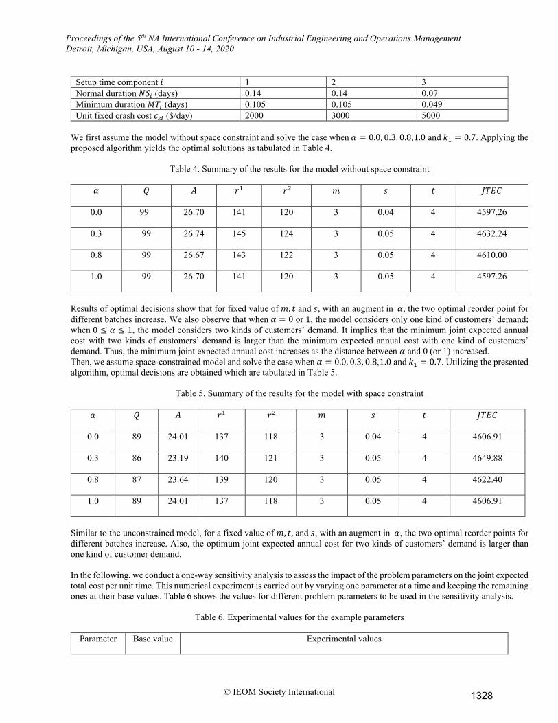
Setup time component 𝑖𝑖 1 2 3 Normal duration 𝑁𝑁𝑆𝑆𝑖𝑖 (days) 0.14 0.14 0.07 Minimum duration 𝑀𝑀𝑇𝑇𝑖𝑖 (days) 0.105 0.105 0.049 Unit fixed crash cost 𝑐𝑐𝑠𝑠𝑖𝑖 ($/day) 2000 3000 5000
We first assume the model without space constraint and solve the case when 𝛼𝛼 = 0.0, 0.3, 0.8,1.0 and 𝑘𝑘1 = 0.7. Applying the proposed algorithm yields the optimal solutions as tabulated in Table 4.
Table 4. Summary of the results for the model without space constraint
𝛼𝛼 𝑄𝑄
𝐴𝐴 𝑟𝑟1 𝑟𝑟2 𝑚𝑚 𝑠𝑠 𝑡𝑡 𝐽𝐽𝑇𝑇𝐸𝐸𝐶𝐶
0.0 99 26.70 141
120
3
0.04 4
4597.26
0.3
99 26.74 145 124 3 0.05
4 4632.24
0.8
99 26.67 143 122
3
0.05 4
4610.00
1.0
99 26.70 141 120
3 0.05 4 4597.26
Results of optimal decisions show that for fixed value of 𝑚𝑚, 𝑡𝑡 and 𝑠𝑠, with an augment in 𝛼𝛼, the two optimal reorder point for different batches increase. We also observe that when 𝛼𝛼 = 0 or 1, the model considers only one kind of customers’ demand; when 0 ≤ 𝛼𝛼 ≤ 1, the model considers two kinds of customers’ demand. It implies that the minimum joint expected annual cost with two kinds of customers’ demand is larger than the minimum expected annual cost with one kind of customers’ demand. Thus, the minimum joint expected annual cost increases as the distance between 𝛼𝛼 and 0 (or 1) increased. Then, we assume space-constrained model and solve the case when 𝛼𝛼 = 0.0, 0.3, 0.8,1.0 and 𝑘𝑘1 = 0.7. Utilizing the presented algorithm, optimal decisions are obtained which are tabulated in Table 5.
Table 5. Summary of the results for the model with space constraint
𝛼𝛼 𝑄𝑄
𝐴𝐴 𝑟𝑟1 𝑟𝑟2 𝑚𝑚 𝑠𝑠 𝑡𝑡 𝐽𝐽𝑇𝑇𝐸𝐸𝐶𝐶
0.0 89 24.01
137 118
3
0.04 4
4606.91
0.3
86 23.19
140 121
3 0.05
4 4649.88
0.8
87 23.64 139 120
3
0.05 4
4622.40
1.0
89 24.01 137 118 3 0.05 4 4606.91
Similar to the unconstrained model, for a fixed value of 𝑚𝑚, 𝑡𝑡, and 𝑠𝑠, with an augment in 𝛼𝛼, the two optimal reorder points for different batches increase. Also, the optimum joint expected annual cost for two kinds of customers’ demand is larger than one kind of customer demand. In the following, we conduct a one-way sensitivity analysis to assess the impact of the problem parameters on the joint expected total cost per unit time. This numerical experiment is carried out by varying one parameter at a time and keeping the remaining ones at their base values. Table 6 shows the values for different problem parameters to be used in the sensitivity analysis.
Table 6. Experimental values for the example parameters
Parameter
Base value Experimental values
1328

Proceedings of the 5th NA International Conference on Industrial Engineering and Operations Management Detroit, Michigan, USA, August 10 - 14, 2020
© IEOM Society International
𝐷𝐷 624 500 550 624 650 700 750 𝛾𝛾(𝑎𝑎, 𝑏𝑏) 𝛾𝛾(10,40) 𝛾𝛾(10,70) 𝛾𝛾(10,50) 𝛾𝛾(10,40) 𝛾𝛾(10,30) 𝛾𝛾(10,20) 𝛾𝛾(25,60) 𝜎𝜎 15 5 10 15 20 25 30 ℎ𝑣𝑣 3 1 2 3 4 5 6 𝐹𝐹 400 300 350 400 450 500 550 𝜋𝜋 70 50 60 70 80 90 100 ℎ𝑏𝑏1 10 5 7 10 12 14 15 ℎ𝑏𝑏2 5 2 4 5 7 9 10 𝐴𝐴0 50 20 30 50 60 80 100 𝑆𝑆𝑐𝑐 1 0.5 0.75 1 1.25 1.5 1.75 𝛿𝛿 1/700 1/400 1/600 1/700 1/1000 1/1200 1/1400 𝑎𝑎 1000 500 750 1000 1250 1500 1750 𝑚𝑚 7 4 6 7 9 11 13
Figure 1. displays graphically the results of the sensitivity study as a tornado diagram, which shows how the joint expected total cost per unit time changes while the problem parameters are independently varied from their low to high values. The length of each bar in the diagram represents the extent to which the expected joint total cost per unit time is sensitive to the bar’s corresponding problem parameter. It can be observed from Fig. 1 that the problem parameters with the greatest impact on the model’s expected cost is defective rate. With other parameters held at their base values, when defective rate is varied from 𝛾𝛾(10,70) to 𝛾𝛾(2,6), the value of the joint expected cost per unit time changed from 3517 to 5849. This shows a larger amount of defective rate can be highly affect the joint expected total cost. Other problem parameters which have largest impact on joint expected cost are average demand per unit time and buyer’s demand standard deviation. Therefore, the inventory decision maker must carefully estimate the values of these parameters since they have most significant effect on the model’s cost.
Figure 1. Sensitivity analysis results 5. Conclusion The purpose of this paper is to propose a multi-reorder level inventory-production model in which the buyer’s LTD follows the mixture of distributions. The paper assumes the buyer’s maximum permissible storage space is limited and therefore adds a space constraint to the respective inventory system. It is also assumed that each lot received contains percentage defectives with a known probability density function. Lead time components and ordering cost are considered to be controllable. A Lagrangian method is utilized to solve the model, and a solution procedure is proposed to find optimal values. The behavior of the model is illustrated in numerical examples. Results of optimal decisions show that for a fixed value of 𝑚𝑚, 𝑡𝑡 and 𝑠𝑠, with an augment in 𝛼𝛼, the two optimal reorder points for different batches increase. We also observe that when 𝛼𝛼 = 0 or 1, the model considers only one kind of customers’ demand; when 0 ≤ 𝛼𝛼 ≤ 1, the model considers two kinds of customers’ demand. It implies that the minimum joint expected annual cost with two kinds of customers’ demand is larger than the minimum expected annual cost with one kind of customer demand. Thus, the minimum joint expected annual cost increases as the distance between 𝛼𝛼 and 0 (or 1) increased. To increase the scope of our analysis, the model presented in this article could be
1329

Proceedings of the 5th NA International Conference on Industrial Engineering and Operations Management Detroit, Michigan, USA, August 10 - 14, 2020
© IEOM Society International
extended in several ways. For example, shortage cost can be calculated as a mixture of backorder and lost sales. Thus, with an increasing or a decreasing in a backorder rate, the optimal order quantity and reorder level may be higher or lower. Also, investigating on some other LTD approach such as gamma and lognormal distribution could be considered. Other kind of constraints such as budget constraint could be added to make the system closer to real environment. References Banerjee, A. (1986). Economic-lot-size model for purchaser and vendor. Decis. Sci, 17, 292–311. Chang, H.-C., Ouyang, L.-Y., Wu, K.-S., & Ho, C.-H. (2006). Integrated vendor–buyer cooperative inventory models with
controllable lead time and ordering cost reduction. European Journal of Operational Research, 170(2), 481–495. Charnes, A., & Cooper, W. W. (1959). Chance-Constrained Programming. Management Science, 6(1), 73–79. Fazeli, S. S., Venkatachalam, S., Chinnam, R. B., & Murat, A. (2020). Two-Stage Stochastic Choice Modeling Approach for
Electric Vehicle Charging Station Network Design in Urban Communities. IEEE Transactions on Intelligent Transportation Systems, 1–16.
Goyal, S. K. (1977). An integrated inventory model for a single supplier-single customer problem. International Journal of Production Research, 15(1), 107–111.
Haksever, C., & Moussourakis, J. (2005). A model for optimizing multi-product inventory systems with multiple constraints. International Journal of Production Economics, 97(1), 18–30.
Hariga, M. A. (2010). A single-item continuous review inventory problem with space restriction. International Journal of Production Economics, 128(1), 153–158.
Ho, C.-H. (2009). A minimax distribution free procedure for an integrated inventory model with defective goods and stochastic lead time demand. International Journal of Information and Management Sciences, 20, 161–171.
Hsiao, Y. C. (2008). A note on integrated single vendor single buyer model with stochastic demand and variable lead time. International Journal of Production Economics, 114(1), 294–297.
Huang, C.-K. (2002). An integrated vendor-buyer cooperative inventory model for items with imperfect quality. Production Planning & Control, 13(4), 355–361.
Lee, W. C., Wu, J. W., & Hou, W. Bin. (2004). A note on inventory model involving variable lead time with defective units for mixtures of distribution. International Journal of Production Economics, 89(1), 31–44.
Liao, C., & Shyu, C. (1991). An Analytical Determination of Lead Time with Normal Demand. International Journal of Operations & Production Management, 11(9), 72–78.
Lou, K.-R., & Wang, W.-C. (2013). A comprehensive extension of an integrated inventory model with ordering cost reduction and permissible delay in payments. Applied Mathematical Modelling, 37(7), 4709–4716.
Moon, I., & Ha, B.-H. (2012). Inventory systems with variable capacity. European Journal of Industrial Engineering, 6(1), 68–86.
Ouyang, L. Y., Wu, K. S., & Ho, C. H. (2004). Integrated vendor-buyer cooperative models with stochastic demand in controllable lead time. International Journal of Production Economics, 92(3), 255–266.
Porteus, E. L. (1985). Investing in Reduced Setups in the EOQ Model. Management Science, 31(8), 998–1010. Ross, S. (1996). Stochastic Processes (2nd ed). Wiley. Tahami, H., Mirzazadeh, A., Arshadi-Khamseh, A., & Gholami-Qadikolaei, A. (2016). A periodic review integrated
inventory model for buyer’s unidentified protection interval demand distribution. Cogent Engineering, 3(1). Tahami, H., Mirzazadeh, A., & Gholami-Qadikolaei, A. (2019). Simultaneous control on lead time elements and ordering
cost for an inflationary inventory-production model with mixture of normal distributions LTD under finite capacity. RAIRO-Oper. Res., 53(4), 1357–1384.
Veinott, A. (1965). Optimal Policy for a Multi-Product, Dynamic, Nonstationary Inventory Problem. Management Science, 12(3), 206–222.
Yahoodik, S., Tahami, H., Unverricht, J., Yamani, Y., Handley, H., & Thompson, D. (2020). Blink Rate as a Measure of Driver Workload during Simulated Driving. Proceedings of the Human Factors and Ergonomics Society 2020 Annual Meeting, Chicago, IL.
Hesamoddin Tahami is a Ph.D. candidate in Engineering Management & Systems Engineering department at Old Dominion University. He received his B.S. and M.S. degree in Industrial & Systems Engineering. His area of research includes Supply chain optimization, Transportation, Humanitarian Logistics, and Data analysis. Hengameh Fakhravar is a Ph.D. student in Engineering Management & Systems Engineering department at Old Dominion University. She received her B.S. and M.S. degree in Industrial & Systems Engineering. Her research interests are Statistical analysis, Fuzzy methods, and System engineering.
1330
Recommended