Download pdf - Multi-Scale Sampling to Evaluate Assemblage Dynamics in an ... · Multi-scale, spatially explicit sampling and analysis was necessary to interpret assemblage dynamics in the CCA and

Multi-Scale Sampling to Evaluate Assemblage Dynamicsin an Oceanic Marine ReserveAndrew R. Thompson*, William Watson, Sam McClatchie, Edward D. Weber

Fisheries Resources Division, Southwest Fisheries Science Center, National Marine Fisheries Service, National Oceanic and Atmospheric Administration (NOAA), La Jolla,

California, United States of America

Abstract

To resolve the capacity of Marine Protected Areas (MPA) to enhance fish productivity it is first necessary to understand howenvironmental conditions affect the distribution and abundance of fishes independent of potential reserve effects. Baselinefish production was examined from 2002–2004 through ichthyoplankton sampling in a large (10,878 km2) SouthernCalifornian oceanic marine reserve, the Cowcod Conservation Area (CCA) that was established in 2001, and the SouthernCalifornia Bight as a whole (238,000 km2 CalCOFI sampling domain). The CCA assemblage changed through time as theimportance of oceanic-pelagic species decreased between 2002 (La Nina) and 2003 (El Nino) and then increased in 2004 (ElNino), while oceanic species and rockfishes displayed the opposite pattern. By contrast, the CalCOFI assemblage wasrelatively stable through time. Depth, temperature, and zooplankton explained more of the variability in assemblagestructure at the CalCOFI scale than they did at the CCA scale. CalCOFI sampling revealed that oceanic species impingedupon the CCA between 2002 and 2003 in association with warmer offshore waters, thus explaining the increased influenceof these species in the CCA during the El Nino years. Multi-scale, spatially explicit sampling and analysis was necessary tointerpret assemblage dynamics in the CCA and likely will be needed to evaluate other focal oceanic marine reservesthroughout the world.

Citation: Thompson AR, Watson W, McClatchie S, Weber ED (2012) Multi-Scale Sampling to Evaluate Assemblage Dynamics in an Oceanic Marine Reserve. PLoSONE 7(3): e33131. doi:10.1371/journal.pone.0033131

Editor: Simon Thrush, National Institute of Water & Atmospheric Research, New Zealand

Received November 10, 2011; Accepted February 5, 2012; Published March 20, 2012

This is an open-access article, free of all copyright, and may be freely reproduced, distributed, transmitted, modified, built upon, or otherwise used by anyone forany lawful purpose. The work is made available under the Creative Commons CC0 public domain dedication.

Funding: This research was funded by the National Marine Fisheries Service. The funders had no role in study design, data collection and analysis, decision topublish, or preparation of the manuscript.

Competing Interests: The authors have declared that no competing interests exist.

* E-mail: [email protected]

Introduction

Marine protected areas (MPAs) potentially influence the

dynamics of multiple species because protection from anthropo-

genic activity is extended, at least to some degree, to all species

residing within a geographically bound region. A first step towards

understanding the role of MPAs in an ecosystem context is to

characterize baseline species assemblages that utilize a reserve and

to evaluate how assemblages of species change through time.

An overarching objective of most MPA-based management

plans is to augment regional fisheries productivity [1]. Given the

diversity of habitats utilized by fishes within and around many

MPAs, collecting quantitative, replicable data on multiple species

is a major challenge for evaluating the dynamics of species

assemblages. This constraint can be overcome to a large extent by

collecting fishery independent data such as abundance of early life

stages of fishes (i.e., ichthyoplankton). Because ichthyoplankton

reflect fish spawning stock biomass [2,3] this method of sampling

has the potential to assess directly whether MPAs impact fishery

production from local to regional scales. Determining whether

MPAs impact larval output can be complicated, however, because

fluctuating environmental conditions are known to induce

variability in fish spawning activity independent of reserve effects.

To disentangle the impact of underlying environmental dynamics

from the influence of MPAs on reproductive output it is necessary

to first elucidate how environmental variability affects ichthyo-

plankton.

Oceanic MPAs are by definition nested within an open, advective

system. Although the extent of MPA boundaries are static the spatial

extent of water masses can change dramatically among years [4,5]

introducing distinct assemblages of pelagic fishes [6] and zooplank-

ton [7]. It is therefore likely that large-scale oceanographic processes

will influence local assemblages within an oceanic MPA in a way that

is not reflected solely at the local scale. Thus, a potentially fruitful

approach for monitoring assemblage dynamics in an oceanic MPA is

to couple detailed, focused sampling within the MPA with broader

sampling to monitor the larger region encompassing the MPA.

The Cowcod Conservation Area (CCA; Fig. 1A) is the largest

MPA in Southern California and the only one that includes

extensive oceanic and nearshore habitats [8]. The CCA is

embedded within the California Cooperative Oceanic Fisheries

Investigations (CalCOFI) sampling domain where ichthyoplank-

ton have been sampled regularly since 1951 at sixty-six stations

including five within the CCA (Fig. 1B). Although analysis of

CalCOFI data provided insight on ichthyoplankton dynamics at

the scale of the SCB over decadal time periods (e.g., [9,10])

understanding of spatial and temporal patterns at finer scales

within the CalCOFI domain is limited (but see [11,12]). To

characterize baseline ichthyoplankton assemblages within the

CCA, fine-scale surveys were conducted in the winters of the

three years (2002–2004) following establishment.

Here, we analyze the CCA data and accompanying CalCOFI

data to determine how assemblage dynamics at the larger scale

compared with the smaller CCA scale and discern how large scale

PLoS ONE | www.plosone.org 1 March 2012 | Volume 7 | Issue 3 | e33131

dynamics affected the fish assemblage at the smaller scale. This

study occurred during a transition from La Nina (2002) to El Nino

(2003, 2004) conditions [13] which enabled us to assess how

fluctuating ocean conditions affected within- and between-year

assemblage structure at both spatial scales.

Methods

Ethics StatementCollections were made pursuant to a Memorandum of

Understanding (MOU) by and between the California Depart-

ment of Fish and Game, National Oceanic and Atmospheric

Administration (NOAA)/National Marine Fisheries Service

(NMFS)/Southwest Region, and NOAA/NMFS/Southwest Fish-

eries Science Center dated 11 February 1986 in a manner that

ameliorated suffering of specimens.

Study area and sample designThe CCA is a restricted-fishing zone that was established in

2001 in response to population declines of the cowcod rockfish

(Sebastes levis) [8]. It consists of an approximately 10,878 km2

western (Figs. 1A, B) and 260 km2 eastern area (Fig. 1B). Our

Figure 1. Maps showing the multi-scale sampling domains and locations where samples were collected. (A) Cowcod Conservation Area(CCA) sampling domain. Triangles depict sample sites, and the white line delineates the border of the western CCA. (B) CalCOFI sampling domain.Circles indicate the location of CalCOFI sample sites, triangles the location of CCA sample sites, and white lines the borders of the western and easternCCAs. The red rectangle in the inset figure delineates the geographic boundary of the area in (B) relative to a broader view of western North America.doi:10.1371/journal.pone.0033131.g001

Larval Fish Assemblages at Multiple Scales


analysis focused on the spatially-continuous western CCA

(henceforth CCA; Fig. 1A). Within the CCA it is illegal to fish

in waters deeper than 36 m. Although the CCA is entirely on the

continental shelf, bottom depths are quite heterogeneous, ranging

from sea level at the shores of San Nicholas and Santa Barbara

Islands to near 2000 m in multiple basins.

Ichthyoplankton and oceanographic data were collected at two

spatial scales: the focal CCA (Fig. 1A), and the larger,

approximately 238,000 km2, California Cooperative Oceanic

Fisheries Investigations (CalCOFI; see [14] for a description of

the CalCOFI program) area that encompasses the CCA (Fig. 1B).

At both scales sample sites were arranged in a grid with

longitudinally separated lines running roughly perpendicular to

shore. Sixty-six locations were sampled within the CCA each year

with adjacent sample sites separated by approximately 9.5 and

18 km in longitudinal and latitudinal directions, respectively.

Measurements were also taken from sixty-six locations at the

CalCOFI scale. These sites constitute the ‘‘core’’ CalCOFI

stations that have been sampled regularly since 1951 [15].

Adjacent CalCOFI lines were 74-km apart. Within lines, stations

were unequally spaced as adjacent sample locations on the

continental shelf were closer to one another (10 to 37 km) than

seaward stations (74 km) (Fig. 1B).

Icthyoplankton samples and environmental measurements were

collected annually in the winters of 2002, 2003, and 2004, during

the peak rockfish (Sebastes spp.) reproductive period [16]. In 2002

samples at both scales were taken between 24 January and 11

February and in 2003 between 30 January and 15 February. In

2004 the CalCOFI sites were sampled prior (January 5–20) to the

CCA sites (February 10–16). Data were collected continuously day

and night.

The standard CalCOFI bongo net (71-cm diameter openings,

0.505 mm mesh nets, detachable 0.333 mm mesh cod ends; [11])

protocol was used to sample ichthyoplankton at all site [17]. A

flowmeter attached to the net measured volume of filtered water.

Samples were preserved in 5% formalin buffered with sodium

borate, and all fish larvae were identified to the lowest possible

taxonomic level in the laboratory. Most taxa were identified to

species (Table S1) but, with the exception of Sebastes jordani, S.

paucispinis, and S. levis, rockfish larvae are morphologically

indistinguishable and were identified to genus (Sebastes spp.). The

number of fish larvae under 10 m2 surface area (to the maximum

depth of a haul) was calculated for each taxon following the

standard CalCOFI methodology [18].

Four environmental covariates were sampled at each site. Sea

surface temperature (SST) and bottom depth (depth) were taken

Figure 2. Interannual environmental variation at both scales. (A) Mean (62SE) sea surface temperature; (B) Zooplankton volume. The filledcircles are from the CCA and the open squares from the CalCOFI sample domains.doi:10.1371/journal.pone.0033131.g002



directly from ship instruments at the initiation of each haul. Small

macrozooplankton displacement volume (henceforth ‘‘zooplank-

ton’’) was calculated for each sample (ml of plankton displacement

per 1000 m3 of filtered water) [19]. We also estimated chlorophyll

a values based on satellite imagery for the 30-day period

encompassing each survey. This variable, however, was consis-

tently highly correlated with at least one of the other covariates,

and we therefore excluded chlorophyll a from further analysis.

Environmental VariabilityWe expected that the ichthyoplankton assemblage would be

affected by oceanographic conditions that changed between the

2002 La Nina and 2003–2004 El Nino [13]. We determined if

SST and zooplankton within our sample frames reflected

oceanographic conditions expected during La Nina (cool SST,

high zooplankton) and El Nino (high SST, low zooplankton) years

in the Southern California region [15] and whether the sampling

perspective affected the patterns.

Change in assemblage structureTo help visualize assemblage dynamics among years we first

performed separate principle components analyses (PCA) on the

site by species matrices from the CCA and CalCOFI scales and

plotted site scores from the first two PC axes (PC1 and PC2). We

then used redundancy analysis (RDA) to determine if there were

differences in assemblage structure between years at the CCA

and CalCOFI sample domains. Sample year was treated as a

discrete variable and overall significance was assessed at a= 0.05

based on 1000 permutations of the data. If an overall difference

was detected, comparisons between pairs of continuous years

were made with significance levels adjusted to account for

multiple comparisons (a= 0.017). Adjusted R2 [20] values were

also reported to quantify the unbiased coefficient of determina-

tion for each test. Prior to this and all other analyses on

assemblages (see below) taxa were removed that were not found

in at least 5% of the samples and stations were taken out that

contained less than three individual larvae. One station was

removed from the 2003 CalCOFI data set and nine from the

2004 CalCOFI analysis due to the low (0 or 1) number of

captured larvae. Fish abundances were Hellinger-transformed

prior to ordination because this transformation has been shown to

produce unbiased results in Euclidian-based multivariate analysis

such as PCA and RDA when zero species counts are prevalent

[21].

Effect of covariates on interannual dynamicsWe discerned the individual and combined effects of SST,

zooplankton, depth, and year on CCA and CalCOFI assemblage

dynamics. First, to evaluate the effects of the covariates on an

entire assemblage, we conducted variance partitioning of scale-

specific RDAs that modeled the covariates SST, zooplankton,

depth and time against assemblage structure [20]. We included

time as a distinct, categorical covariate to ascertain how much

variance was explained by year of sampling that was not

attributable to the sampled environmental parameters. Second,

to better elucidate the dynamics of particular groups of species, we

extracted the first two PC eigenvectors from the unconstrained,

scale-specific PCAs that were based on the site by species matrices.

We then used linear models to calculate how much of the variation

in PC1 and PC2 was explained by the covariates. Finally, we used

variance partitioning to ascertain the unique and shared

contribution of each covariate to the explained variation of PC

1 and PC2 at each scale.

Effect of covariates on within-year distributionsWe analyzed the horizontal distribution of assemblages within

each year at both scales. We again evaluated how well covariates

explained year-specific assemblage structure first using RDA and

second linear models of PC1 and PC2 from PCAs of the site by

species matrix from each assemblage at both scales. We then used

variance partitioning to determine the amount of variation that

was explained by each covariate. In addition to the environmental

covariates (depth, SST and zooplankton) we included in these

analyses spatial covariates. Spatial covariates provide insight

towards processes affecting species distribution because they

identify nonrandom distribution patterns that are not fully

explained by the measured environmental covariates [21]. Such

spatial effects indicate that unmeasured endogenous (i.e., behav-

ioral or ecological) or exogenous (i.e., environmental parameters)

processes affect an assemblage, and/or there is a mismatch

between the scale of sampling and the response of species to

environmental variables [22–24]. Thus, spatial covariates provide

Figure 3. Variability in assemblage structure among years atboth scales. Scores of PC1 and PC2 of each station from 2002 (circles),2003 (triangles), and 2004 (diamonds) are shown for the (A) CCA and (B)CalCofi scales. See Table 2 for taxa loadings on each axis.doi:10.1371/journal.pone.0033131.g003



Table 1. Frequency of occurrence, mean abundance, and proportion of abundance constituted by individual ichthyoplankton taxafor each sample year within the CCA and CalCOFI sampling domains.

CCA Domain CalCOFI Domain

Frequency ofOccurrence Mean Abundance


Taxon scientific name common name 2002 2003 2004 2002 2003 2004 2002 2003 2004 2002 2003 2004

Clupeidae

Sardinops sagax Pacific sardine 0.09 0.01 0.13 32.85 0.07 0.81 0 0.03 0 0 0.36 0

Engraulidae

Engraulis mordax Northernanchovy

0.91 0.31 0.63 302.72 24.26 15.60 0.35 0.29 0.08 12.80 18.49 0.51

Argentinidae

Argentina sialis Pacific argentine 0.20 0.01 0.09 1.04 0.08 0.51 0.03 0.02 0.05 0.22 0.07 0.29

Bathylagidae

Leuroglossus stilbius Cal.smoothtongue

1.00 0.79 0.91 286.04 29.01 47.84 0.63 0.28 0.30 52.74 4.29 13.80

Lipolagus ochotensis Popeyeblacksmelt

0.92 0.81 0.94 44.32 11.81 31.37 0.66 0.37 0.31 30.85 3.24 8.59

Gonostomatidae

Cyclothone signata Showybristlemouth

0 0.09 0.09 0 0.72 0.65 0.08 0.15 0.17 0.68 1.67 1.14

Sternoptychidae

Argyropelecus sladeni Lowcresthatchetfish

0.18 0.04 0.04 1.02 0.22 0.21 0.12 0.08 0.06 0.98 0.42 0.44

Danaphos oculatus Bottlelight 0.09 0.07 0.13 0.45 0.46 0.73 0.12 0.09 0.11 1.24 0.42 0.77

Phosichthyidae

Vinciguerria lucetia Panama lightfish 0.02 0.01 0.07 0.07 0.07 0.71 0.18 0.18 0.08 4.61 3.27 0.42

Stomiidae

Stomias atriventer Blackbellydragonfish

0.08 0.04 0.10 0.59 0.24 0.49 0.02 0.06 0.02 0.16 0.28 0.07

Idiacanthidae

Idiacanthusantrostomus

Pacificblackdragon

0 0.01 0 0 0.08 0 0.12 0.05 0.06 0.76 0.34 0.28

Paralepididae

Lestidiops ringens Slenderbarracudina

0.02 0.16 0.12 0.07 0.95 0.56 0.05 0.14 0.03 0.29 0.68 0.20

Myctophidae

Ceratoscopelustownsendi

Dogtoothlampfish

0 0 0 0 0 0 0.11 0.09 0.02 1.43 0.49 0.07

Nannobrachiumritteri

Broadfinlampfish

0.27 0.49 0.33 2.04 4.76 3.36 0.15 0.34 0.27 1.53 4.23 2.17

Stenobrachiusleucopsarus

Northernlampfish

0.98 0.93 0.99 148.66 53.10 69.53 0.62 0.66 0.50 44.45 24.50 18.76

Diogenichthysatlanticus

Longfinlanternfish

0.08 0.34 0.28 0.45 2.29 1.55 0.25 0.29 0.25 5.76 3.27 2.26

Protomyctophumcrockeri

Cal. flashlightfish 0.59 0.46 0.43 7.59 4.47 3.81 0.48 0.49 0.45 7.33 6.72 4.23

Symbolophoruscaliforniensis

Cal. lanternfish 0 0.15 0.13 0 1.13 0.88 0.12 0.25 0.13 1.54 3.20 1.29

Tarletonbeaniacrenularis

Blue lanternfish 0.42 0.27 0.04 3.49 2.19 0.20 0.20 0.15 0.08 2.49 1.01 0.56

Merlucciidae

Merluccius productus Pacific hake 1.00 0.27 0.97 252.80 8.79 117.29 0.62 0.14 0.19 338.59 1.42 9.23

Scorpaenidae

Sebastes aurora Aurora rockfish 0.15 0.06 0.10 0.94 0.62 0.73 0.02 0.02 0 0.30 0.07 0



valuable clues regarding processes that affect assemblages that are

not identified by the sampled environmental variables [24].

Spatial covariates were generated specifically for the CCA and

CalCOFI domains using the principle coordinates of neighbor

matrices (PCNM) method. PCNM produces eigenvectors based on

a connectivity matrix (minimum spanning tree) of the geographical

coordinates of sample sites (see Figure 1 in [25] for an illustration

that describes the derivation of PCNM eigenvectors). The resultant

spatial covariates (PCNM variables) depict spatial relationships

among sample sites at a continuum of spatial scales within the

bounds of the sample area [21]. PCNM variables with large

eigenvalues describe broad-scale spatial relationships and vice versa.

We utilized a conservative approach for including PCNM variables

in the analyses to avoid overfitting [26]. We reduced the number of

PCNM variables by using a conservative forward selection technique

based on adjusted R2 values and a cutoff of p = 0.05 [27] and limited

to five the number of PCNM variables in any one analysis [28].

PCA, RDA, variance partitioning, and forward selection

analyses were carried out using the statistical software R version

2.11.0 with the packages Vegan 1.17–2 [29] and packfor [27]. We

generated PCNM eigenvectors using SAM v4.0 [30]. Maps were

produced using ArcGIS version 10.0.

Results

Environmental dynamicsInterannual patterns of SST and zooplankton conformed to

previous findings of low SST and high zooplankton during a La

Nina and vice versa during an El Nino [15] at the large CalCOFI

scale in each year, and at the smaller CCA scale in 2002 and 2003

but not 2004 (Fig. 2). In the CCA SST increased by an average

(62 SE) of 0.8860.16uC between 2002 and 2003 and then

decreased by 1.1560.14uC between 2003 and 2004 such that the

SST was lowest among the sample years during the 2004 El Nino

(Fig. 2A). At the CalCOFI scale SST also increased from 2002 to

2003 (1.5660.21uC) but decreased only slightly (0.4460.22uC)

from 2003 to 2004 with the lowest average temperature occurring

during the 2002 La Nina (Fig. 2A). Zooplankton consistently

displayed an inverse pattern to SST at both scales (Fig. 2B).

Change in assemblage structureThe larval assemblage was much more dynamic at the smaller

CCA than the larger CalCOFI scale over the three year period

(Fig. 3). Within the CCA the overall RDA model of assemblage

structure versus sample year was highly significant (R2 = 0.23,

p,0.001) as were pairwise comparisons between individual years

(2002 vs 2003 R2 = 0.22, 2003 vs. 2004 R2 = 0.12; p,0.001 for

both). Differences between 2002 and 2003 in the CCA reflected an

increase in the influence of benthic rockfishes (Sebastes spp., S. jordani,

and S. paucispinis) and oceanic species (N. ritteri, P. crockeri, S.

californiensis, D. atlanticus) relative to coastal-oceanic species (E.

mordax, L. stilbius, M. productus) (Table 1; Figs. S1, S2, S3, S4, 3A, 4;

see [31] for the definition of species-specific habitat associations).

From 2003 to 2004 the influence of the oceanic species declined

while that of the coastal-oceanic species increased (Table 1; Figs. S1,

S2, S3, S4, 3A, 4). Although the overall model at the CalCOFI scale

was significant (p,0.01) the coefficient of determination (R2 = 0.02)

Table 1. Cont.

CCA Domain CalCOFI Domain



Taxon scientific name common name 2002 2003 2004 2002 2003 2004 2002 2003 2004 2002 2003 2004

Sebastes goodei Chillipepperrockfish

0.03 0.09 0.19 0.23 0.61 1.66 0.02 0.03 0 0.16 0.13 0

Sebastes jordani Shortbellyrockfish

0.82 0.69 0.87 56.48 39.22 27.95 0.28 0.28 0.14 38.35 8.36 3.04

Sebastes levis Cowcod rockfish 0.11 0.15 0.24 0.88 0.79 2.19 0 0.06 0 0 0.29 0

Sebastes paucispinis Bocaccio rockfish 0.44 0.64 0.84 6.91 8.37 15.51 0.14 0.17 0.11 1.74 1.81 7.08

Sebastes spp. ?? rockfish 0.88 0.94 0.99 250.07 135.34 345.92 0.55 0.43 0.30 43.59 35.59 32.00

Hexagrammidae

Zaniolepis latipinnis Longspinecombfish

0.02 0.03 0.13 0.07 0.15 0.84 0.02 0.02 0 0.15 0.07 0

Crangidae

Trachurussymmetricus

Jack mackerel 0 0.15 0.03 0 1.84 0.23 0.02 0.02 0 0.07 0.36 0

Gobiidae

Rhinogobiopsnicholsii

Blackeye goby 0.30 0.15 0.51 2.14 1.22 3.49 0.02 0.06 0.09 0.15 0.28 0.64

Centrolophidae

Icichthys lockingtoni Medusafish 0.03 0 0.03 0.35 0 0.23 0.12 0.02 0 1.25 0.07 0

Paralichthyidae

Citharichthys sordidus Pacific sanddab 0.44 0.04 0.66 6.94 0.23 9.81 0.34 0.09 0.20 4.72 0.68 1.94

Citharichthysstigmaeus

Speckledsanddab

0.42 0.15 0.43 3.85 0.75 2.93 0.26 0.06 0.08 5.46 0.58 0.73

Only taxa observed in at least 5% of the stations in at least one of the years are shown; a complete list of sampled taxa is provided in Table S1.doi:10.1371/journal.pone.0033131.t001



was much lower than in the CCA. Pairwise comparisons of

CalCOFI years indicated that while the assemblage differed

between 2002 and 2003 (adj R2 = 0.06; p,0.01) it did not change

significantly from 2003 to 2004 (adj R2 = 0.01; p.0.05). The

difference between 2002 and 2003 at the CalCOFI scale was driven

primarily by an increase in the influence of oceanic species (N. ritteri,

P. crockeri, S. californiensis, D. atlanticus) relative to M. productus and

Sebastes spp. in 2003 (Table 1; Figs. S5, S6, S7, S8, 3B, 5).

Effect of covariates on interannual dynamicsThe response of the assemblage to environmental fluctuation

was much more predictable at the larger than the smaller scale.

Variance partitioning of RDA models and linear models of

individual PC axes from the PCAs of the original site by species

matrices (Table 2) showed that environmental parameters

explained much more of the variation in assemblage structure at

the CalCOFI than the CCA scale (Table 3). Further, in the CCA

the amount of variation explained purely by time (i.e., time with

other variables factored out) was greater than that characterized

by the environmental covariates for both the RDA and linear

model of PC1, which characterized a dichotomy between stations

with benthic versus coastal-oceanic taxa (Table 2, 3). At the CCA

scale only SST was relatively effective in describing the variability

of a linear model of PC2 (coastal-oceanic and benthic versus

oceanic taxa; Tables 2, 3). At the CalCOFI scale, by contrast, pure

time was unimportant for all analyses, and the environmental

covariates were particularly effective in explaining the interannual

variability in PC1 (72%), which separated oceanic versus coastal-

oceanic and benthic taxa (Tables 2, 3).

Effect of covariates on within-year distributionsVariance partitioning of models relating environmental and

spatial covariates to assemblage structure at each scale within years

revealed two main findings. First, the amount of variation

explained by the environmental covariates (i.e., depth+SST+zoo-

plankton) measured in the CCA was quite different among years,

ranging from 7 to 22% for the RDA models and 14 to 45% for the

linear models of PC1 (Table 4). At the CalCOFI scale, by contrast,

the amount of variation explained by the environment was

consistently higher as RDA models explained between 17 and

30% and linear models of PC1 between 66 and 79% of the

variance in assemblage structure (Table 4). Second, the amount of

variation explained purely by the spatial covariates (i.e., space with

other covariates factored out) in the RDA models was consistently

similar to the environmental covariates at the CCA scale. At the

CalCOFI scale, however, spatial covariates explained much less of

the variation than the environment for both RDA models and

linear models of PC1 and PC2 (Table 4).

Discussion

The ichthyoplankton assemblage was much more dynamic

within the CCA than the CalCOFI area over the three-year survey

period that was characterized by a transition from La Nina to El

Nino oceanographic conditions. During the La Nina in 2002 the

CCA was dominated by species with coastal-oceanic habitat

affinities (as described by [31]) such as E. mordax, M. productus, and

L. stilbius as well as benthic rockfishes. During the 2003 El Nino,

however, there was a decline in the influence of the coastal-oceanic

species and an increase in rockfishes and several oceanic species

(N. ritteri, D. atlanticus, S. californiensis). In 2004, E. mordax, L. stilbius

and, especially, M. productus, increased (although not to 2002

levels). These results suggest that the coastal-oceanic species

moved out of the CCA between 2002 and 2003 as the oceanic

Ta

ble

2.

Tax

alo

adin

gs

on

the

firs

ttw

op

rin

cip

leco

mp

on

en

tax

es

fro

ma

PC

Ao

fth

esi

teb

ysp

eci

es

mat

rix

of

sam

ple

sfr

om

the

CC

Aan

dC

alC

OFI

sam

plin

gd

om

ain

su

sin

gd

ata

fro

mal

lye

ars.

Sa

mp

leE

ige

n-

Eig

en

-P

rop

ort

ion

Sp

eci

es

wit

hH

ab

ita

tS

pe

cie

sw

ith

Ha

bit

at

Do

ma

inv

ect

or

va

lue

va

ria

nce

Po

siti

ve

loa

din

gs

Aff

init

ies

Ne

ga

tiv

elo

ad

ing

sA

ffin

itie

s

CC

AP

C1

0.1

10

.38

L.st

ilbiu

s(0

.78

),E.

mo

rda

x(0

.61

),M

.p

rod

uct

us

(0.4

8)

coas

tal-

oce

anic

Seb

ast

essp

p.

(21

.21

),S.

jord

an

i(2

0.3

4),

S.p

au

cisp

inis

(20

.27

)b

en

thic

PC

20

.05

0.1

5M

.p

rod

uct

us

(0.8

0),

Seb

ast

essp

p.

(0.3

2),

E.m

ord

ax

(0.2

7),

coas

tal-

oce

anic

,b

en

thic

N.

ritt

eri

(20

.32

),L.

och

ote

nsi

s(2

0.2

6),

P.

cro

cker

i(2

0.2

6),

oce

anic

S.jo

rda

ni

(0.1

2)

S.ca

lifo

rnie

nsi

s(2

.16

),D

.a

tla

nti

cus

(20

.14

)

Cal

CO

FIP

C1

0.1

80

.27

P.

cro

cker

i(0

.77

),D

.a

tla

nti

cus

(0.6

0),

S.ca

lifo

rnie

nsi

s(0

.42

),o

cean

icSe

ba

stes

spp

.(2

0.8

0),

M.

pro

du

ctu

s(2

0.5

1),

L.st

ilbiu

s(2

0.4

0),

coas

tal-

oce

anic

,b

en

thic

V.

luce

tia

(0.4

2),

N.

ritt

eri

(0.3

6),

C.

sig

na

ta(0

.25

)S.

leu

cop

saru

s(2

0.3

9),

E.m

ord

ax

(20

.34

),S.

jord

an

i(2

0.3

2)

PC

20

.10

0.1

5Se

ba

stes

spp

.(0

.70

),S.

jord

an

i(0

.23

),S.

calif

orn

ien

sis

(0.1

9),

E.m

ord

ax

(0.1

7),

D.

atl

an

ticu

s(0

.17

),V

.lu

ceti

a(0

.16

)b

en

thic

,o

cean

ic,

and

coas

tal-

oce

anic

S.le

uco

psa

rus

(20

.69

),L.

och

ote

nsi

s(2

0.6

5),

L.st

ilbiu

s(2

0.2

4)

oce

anic

,co

asta

l-o

cean

ic

Hab

itat

affi

nit

ies

asd

efi

ne

db

y[3

1]

(oce

anic

:N.r

itte

ri,P

.cro

cker

i,S.

calif

orn

ien

sis,

D.a

tla

nti

cus,

S.le

uco

psa

rus;

coas

tal-

oce

anic

:L.

stilb

ius,

L.o

cho

ten

sis,

M.p

rod

uct

us,

E.m

ord

ax;

be

nth

ic:S

eba

stes

spp

.,S.

jord

an

i,S.

pa

uci

spin

is)

of

taxa

wit

hp

osi

tive

and

ne

gat

ive

load

ing

sar

esh

ow

nfo

re

ach

axis

.T

able

1p

rovi

de

sfu

llsp

eci

es

and

com

mo

nn

ame

s.d

oi:1

0.1

37

1/j

ou

rnal

.po

ne

.00

33

13

1.t

00

2



species moved in, and then returned to the area in 2004. They also

highlight how variable the ichthyoplankton assemblage can be in

this region at an annual time scale.

Previous ichthyoplankton research in this area characterized

similar patterns but averaged over longer time frames. Hsieh et al.

[9] examined the distribution and abundance of oceanic (e.g., N.

ritteri, P. crockeri, L. ochotensis, D. atlanticus) and coastal-neritic (e.g., E.

mordax, M. productus, S. sagax) species in association with a regime

shift [4,5] from cool (1950–1976) to warm (1977–1999) conditions.

They found that the abundance of oceanic species expanded and

encroached shoreward during the warm period whereas the

coastal-neritic species retreated shoreward and northward at this

time. Similarly, ichthyoplankton abundances of species with

subtropical affinities increased and moved shoreward throughout

Table 3. Adjusted R2 values from partitioning of the amount of variation explained by depth (D), sea surface temperature (SST),zooplankton volume (Z) and year of sampling (time) for interannual analysis of assemblage structure at the CCA and CalCOFIscales.

SampleDomain Analysis D SST Z Time D+SST D+Z SST+Z D+Z+SST

Pure Time[T | D, SST, Z]

Totalvariationexplained Residuals

CCA RDA 0.05 0.06 0.03 0.23 0.11 0.09 0.06 0.11 0.19 0.30 0.70

linear modelof PC1

0.09 0 0 0.40 0.1 0.1 0.01 0.10 0.42 0.51 0.49

linear modelof PC2

0.08 0.34 0.17 0.34 0.37 0.24 0.35 0.39 0.06 0.45 0.55

CalCOFI RDA 0.14 0.12 0.04 0.02 0.22 0.16 0.12 0.22 0.01 0.23 0.77

linear modelof PC1

0.51 0.43 0.13 0.03 0.72 0.58 0.44 0.72 0.00 0.72 0.28

linear modelof PC2

0.05 0.06 0 0 0.16 0.06 0.06 0.16 0.01 0.17 0.83

Pure time indicates the fraction of variation explained by time after factoring out the shared variation explained by the environmental covariates. PC axes are extractedfrom a PCA of the site by species matrix.doi:10.1371/journal.pone.0033131.t003

Table 4. Adjusted R2 values from partitioning of the amount variation explained by depth (D), sea surface temperature (SST),zooplankton volume (Z) and PCNM eigenvectors (space) for intraannual analysis at the CCA and CalCOFI scales in each sampleyear.

SampleDomain Analysis D SST Z Space D+SST D+Z SST+Z D+Z+SST

Pure Space[S | D, SST, Z]

Totalvariationexplained Residuals

CCA 2002 RDA 0.13 0.12 0.01 0.34 0.18 0.15 0.12 0.22 0.21 0.39 0.61

linear model of PC1 0.31 0.32 0 0.49 0.45 0.34 0.31 0.45 0.16 0.61 0.39

linear model of PC2 0.05 0 0.00 0.45 0.04 0.04 0 0.02 0.44 0.46 0.53

CCA 2003 RDA 0.02 0.03 0.02 0.17 0.05 0.04 0.05 0.07 0.11 0.17 0.82

linear model of PC1 0.03 0.06 0.05 0.30 0.10 0.08 0.12 0.14 0.00 0.14 0.86


CCA 2004 RDA 0.08 0.02 0.01 0.14 0.10 0.09 0.03 0.10 0.11 0.21 0.79



CalCOFI 2002 RDA 0.14 0.16 0.07 0.23 0.24 0.18 0.16 0.24 0.09 0.33 0.67



CalCOFI 2003 RDA 0.23 0.10 0.04 0.26 0.30 0.23 0.13 0.30 0.03 0.33 0.67



CalCOFI 2004 RDA 0.11 0.15 0.00 0.21 0.18 0.10 0.15 0.17 0.06 0.23 0.77



Pure space indicates the fraction of variation explained by the spatial covariates after factoring out the shared variation explained by the environmental covariates. PCaxes are extracted from a PCA of the site by species matrix.doi:10.1371/journal.pone.0033131.t004



California and Baja California, Mexico, following a transition

from cool, La Nina conditions in 1954–56 to warm, El Nino

conditions in 1958–1959 [32]. Our results build on these analyses

of longer time series by demonstrating how abruptly the

ichthyoplankton assemblages can change over a relatively short

time frame.

Comparison of the relationship between covariates and

assemblage structure at the CCA and CalCOFI scales revealed

two main points. First, although the CCA assemblage changed

through time, the sampled environmental variables explained

relatively little of the variation. At the CalCOFI scale, however,

environmental covariates better explained the dynamics of the

assemblage. Second, purely temporal (year) and spatial (PCNM)

covariates consistently explained more of the variation in

assemblage structure than the measured environmental covariates

at the CCA scale, but the opposite was true at the CalCOFI scale.

These results may be caused by multiple nonexclusive factors [33].

One possibility is that the variation captured by year and

unexplained spatial covariates within the CCA was induced by

unmeasured environmental factors such as salinity [34], mixed

layer depth [35] or dissolved oxygen concentration [10]. Another

possibility is that the unexplained time and space variables were

proxies for biological interactions. Biological processes such as

schooling behavior, competition, and migration/dispersal can

induce spatial clustering independent of environmental effects

either by concentrating species within a small portion of suitable

habitat or by causing species to occupy suboptimal habitat [33].

Because most of the larvae captured in our study were in the very

early stages of development and were poor swimmers it is unlikely

that behavioral processes had a large effect on horizontal

distribution. However, if behavior influenced the distribution of

spawning adults then biological interactions could be reflected in

larval distributions.

A third possibility is that there was a mismatch between the

scale of sampling within the CCA and the response of species to

environmental variability. This explanation is supported by recent

theoretical work indicating that if species respond to environmen-

tal fluctuation at a scale larger or smaller than a sample frame,

then there is a tendency for the amount of variation that is

explained by spatial covariates to increase relative to environmen-

tal parameters [23]. In our case, it is possible that at least the

pelagic species responded to environmental variability at a scale

that more closely matched the CalCOFI than the CCA sampling

domain. For example, the range of SST across the CalCOFI

region was 11.5–17.2uC during the study period but across the

CCA it was only between 12.7 and 16.2uC. The relatively narrow

range of temperatures encountered in the CCA likely had more

subtle effects on fish distributions than did the large range of

temperatures across the CalCOFI region. In particular, examina-

tion of the assemblage from the CalCOFI scale suggests that the

assemblage was affected by shifting water mass boundaries as PC1

scores correlated highly with SST. CalCOFI PC1 separated

stations characterized by taxa with oceanic affinities (e.g., N. ritteri,

P. crockeri, and S. californiensis) from those with coastal-pelagic and

benthic habitat association (e.g., Sebastses spp., E. mordax, S.

leucopsarus and M. productus), and the distribution of these taxa

shifted among years. In 2002 stations with high PC1 scores (i.e.,

oceanic species) clustered in the southwest portion of the sample

domain. In addition, stations west of the shelf in the northern part

of the CalCOFI domain contained coastal species, suggesting

offshelf transport in 2002, a pattern also identified for S. sagax in

spring of that year [13]. In 2003, by contrast, oceanic species

impinged upon the shelf and into the CCA together with warmer

water. Despite the large-scale movement of warm water and

broad-scale warming in 2003 and 2004 relative to 2002, SST in

the CCA was actually lower in 2004 than 2002, perhaps reflecting

local upwelling in 2004. This discrepancy between large-scale and

local environmental dynamics likely weakened the environment-

species relationship in the CCA.

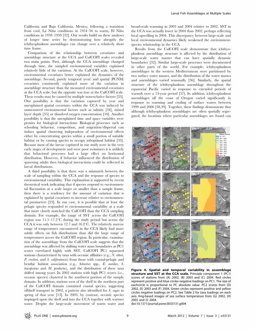
Results from the CalCOFI scale demonstrate that ichthyo-

plankton assemblage structure is affected by the distribution of

large-scale water masses that can have spatially dynamic

boundaries [32]. Similar large-scale processes were documented

in other parts of the world. For example, ichthyoplankton

assemblages in the western Mediterranean were partitioned by

two surface water masses, and the distribution of the water masses

and assemblages varied seasonally [36]. Similarly, the spatial

structure of the ichthyoplankton assemblage throughout the

equatorial Pacific varied in response to extended periods of

warmth over a 13-year period [37]. In addition, ichthyoplankton

assemblages off the coast of Oregon varied significantly in

response to warming and cooling of surface waters between

1999 and 2006 [38,39]. Together, these findings demonstrate that

although ichthyoplankton assemblages are often spatially segre-

gated, the locations where particular assemblages are found can

Figure 4. Spatial and temporal variability in assemblagestructure and SST at the CCA scale. Principle component 1 (PC1)scores of stations from (A) 2002, (B) 2003 and (C) 2004. Red circlesrepresent positive and blue circles negative loadings on PC1. The size ofeachcircle is proportional to PC absolute value. PC2 scores from (D)2002, (E) 2003 and (F) 2004. Green circles represent positive and yellowcircles negative loadings on PC2. See Table 2 for taxa loadings on eachaxis. Krig-based images of sea surface temperature from (G) 2002, (H)2003 and (I) 2004.doi:10.1371/journal.pone.0033131.g004



vary dramatically through time in response to environmental

forcing [40–42].

Although our results suggest that broad-scale processes affected

the CCA assemblage in a way that was not fully apparent by

examining local conditions, there is evidence that local processes

strongly impacted the CCA assemblage in 2002 as environmental

covariates explained more than twice as much variation in this

year than in other years. This result might be driven by

interannual variability in mesoscale oceanographic structure.

The Southern California Bight is bathymetrically heterogeneous

and contains several deep basins with steep vertical drops that can

induce the formation of local fronts (Fig. 1). Nishimoto and

Washburn [43], for example, documented a mesoscale eddy just

north of our study area that affected significantly the distribution

of late-stage fish larvae in 1998 but found no evidence of the eddy

or spatially-structured fish distributions the following year.

Working within the CCA region, McClatchie et al. [12]

documented a strong north-south front that hugged the ridge

south from San Nicholas Island (Fig. 1A) in 2010. This front

separated warm, saline water in the east and cool, fresher water in

the west, and there were different zooplankton, larval fish, and egg

(fish and squid) assemblages on either side of and within the front.

In our study there was a clear east-west gradient in both species

distributions and SST within the CCA in 2002 but less distinct

transitions in other years (Fig. 4, 5). These results suggest that local

oceanographic structure contributed more to assemblage structure

within the CCA in 2002 than other years and imply that both local

and broad-scale oceanographic dynamics can combine to affect

the distribution of ichthyoplankton within the CCA.

These results stress the importance of being cognizant of

sampling scale when describing species-environment relationships

[44]. Although ichthyoplankton studies from around the world

documented differences in assemblage structure from very small

(e.g., ,1-m; [45]) to very large spatial scales (e.g, 4000-km; [6]),

explicit evaluations of assemblage-environment relationships

across sampling scales within a study are rare. Among the existing

multi-scale investigations, Catalan et al. [46] quantified ichthyo-

plankton assemblage structure from a mesoscale sampling grid

(stations separated by 18 km) that was embedded within a

macroscale grid (stations separated by 40 km) off the coast of

Spain and Portugal. Similar to our results they found consistent

differences in assemblage composition between onshelf and offshelf

stations at the macroscale. In addition, they discovered through

mesoscale sampling that the spatial boundary separating assem-

blages was porous as taxa with primarily onshelf affinities were

advected to offshore areas. Another multi-scale study from the

Gulf of Mexico demonstrated that different oceanographic

variables best explained ichthyoplankton distribution patterns at

fine (1-km), meso (10-km) and coarse (100-km) scale sampling

perspectives [47]. These results stress how examining ichthyo-

plankton from multiple perspectives is important given the

inherently dynamic nature of fish distribution.

Ultimately, the aim of future/ongoing research is to compare

icthyoplankton assemblage data reported here with future samples

to ascertain whether the MPA has an effect on the local

production of fishes. Given the findings of this initial effort several

recommendations can be made to augment the efficacy of future

sampling in this and other ichthyoplankton assemblage studies.

First, we found that the CCA assemblage was highly variable at an

annual time scale. However, our results are based on only three

years of sampling and additional annual sampling is necessary to

evaluate how these fluctuations compare to long-term trends.

Second, we showed that assemblages were likely affected by

Figure 5. Spatial and temporal variability in assemblage structure and SST at the CalCOFI scale. Principle component 1 (PC1) scores ofstations from (A) 2002, (B) 2003 and (C) 2004. Red circles represent positive and blue circles negative loadings on PC1. The size of each circle isproportional to PC absolute value. PC2 scores from (D) 2002, (E) 2003 and (F) 2004. Green circles represent positive and yellow circles negativeloadings on PC2. See Table 2 for taxa loadings on each axis. Krig-based images of sea surface temperature from (G) 2002, (H) 2003 and (I) 2004.doi:10.1371/journal.pone.0033131.g005



unmeasured environmental covariates, endogenous behavior by

the species, and/or a mismatch between the scale of sampling and

the response of species to the environment. To better resolve the

relative importance of these factors future sampling needs to

quantify additional oceanographic covariates such as salinity,

current velocity and oxygen in concert with species sampling.

Third, we obtained insight into processes that affected the CCA

assemblage by also sampling at the larger CalCOFI scale. This

result emphasizes the importance of recognizing that oceanic

MPAs are nested in a broader system where forces external to the

reserve can affect assemblage structure within the reserve. Hence,

our results stress the need for multi-scale monitoring to elucidate

the cause of species fluctuation in MPAs. Our findings set the stage

for documentation of the effect of MPAs on fisheries production,

which is a critical, yet largely unresolved question in the study of

MPAs.

Supporting Information

Figure S1 Hellinger-transformed values of oceanicspecies in the CCA from 2002–2004. (A–C) Nanobrachium

ritteri; (D–F) Protomyctophum crockeri; (G–I) Symbolophorous californien-

sis. The white border depicts the boundary of the CCA in this and

all Supplemental Figures. The order in which taxa are presented is

based on their habitat affinities as defined by [31]. The size of a

circle is proportional to its value which ranges between 0 and 1.

(TIF)

Figure S2 Hellinger-transformed values of two oceanicand one coastal-oceanic species in the CCA from 2002–2004. (A–C) Diogenicthys atlanticus (oceanic); (D–F) Stenobrachius

leucopsarus (oceanic); (G–I) Leuroglossus stilbius (coastal-oceanic).

(TIF)

Figure S3 Hellinger-transformed values of coastal-oceanic species in the CCA from 2002–2004. (A–C) Lipolagus

ochotensis; (D–F) Merluccius productus; (G–I) Engraulis mordax.

(TIF)

Figure S4 Hellinger-transformed values of benthic taxain the CCA from 2002–2004. (A–C) Sebastes spp.; (D–F) Sebastes

jordani; (G–I) Sebastes paucispinis.

(TIF)

Figure S5 Hellinger-transformed values of oceanicspecies in the CalCOFI domain from 2002–2004. (A–C)

Nanobrachium ritteri; (D–F) Protomyctophum crockeri; (G–I) Symbolophor-

ous californiensis.

(TIF)

Figure S6 Hellinger-transformed values of two oceanicand one coastal-oceanic species in the CalCOFI domainfrom 2002–2004. (A–C) Diogenicthys atlanticus (oceanic); (D–F)

Stenobrachius leucopsarus (oceanic); (G–I) Leuroglossus stilbius (coastal-

oceanic).

(TIF)

Figure S7 Hellinger-transformed values of coastal-oce-anic species in the CalCOFI domain from 2002–2004. (A–

C) Lipolagus ochotensis; (D–F) Merluccius productus; (G–I) Engraulis

mordax.

(TIF)

Figure S8 Hellinger-transformed values of benthic taxain the CalCOFI domain from 2002–2004. (A–C) Sebastes spp.;

(D–F) Sebastes jordani; (G–I) Sebastes paucispinis.

(TIF)

Table S1 Complete list of taxa sampled in the CowcodConservation Area and CalCOFI.

(DOCX)

Acknowledgments

We extend our thanks to the crews of the ships that collected the data

including D. Abramenkoff, D. Griffith, A. Hays, and S. Manion and the

people who sorted and identified the ichthyoplankton including D.

Ambrose, N. Bowlin, S. Charter, E. Sandknop, and S. Zao. We also

thank K. Stierhoff and R. Cosgrove for assistance on mapping and H. Orr

for help with figure preparation. Comments by K. Stierhoff and an

anonymous reviewer improved the manuscript.

Author Contributions

Conceived and designed the experiments: ART WW SM EDW.

Performed the experiments: ART WW SM EDW. Analyzed the data:

ART WW SM EDW. Contributed reagents/materials/analysis tools: ART

WW. Wrote the paper: ART WW SM EDW.

References

1. Roberts CM, Hawkins JP, Gell FR (2005) The role of marine reserves in

achieving sustainable fisheries. Phil Trans Roy Soc B 360: 123–132.

2. Hunter JR, Lo NC-H, Fuiman LA (1993) Advances in the early life history of

fishes; Part 2, ichthyoplankton methods for estimating fish biomass. Bull Mar Sci

53: 723–935.

3. Ralston S, MacFarlane BR (2010) Population estimation of bocaccio (Sebastes

paucispinis) based on larval production. Can J Fish Aquat Sci 67: 1005–1020.

4. Bograd SJ, Lynn RJ (2003) Long-term variability in the Southern CaliforniaCurrent System. Deep-Sea Res II 50: 2355–2370.

5. McGowan JA, Cayan DR, Dorman LM (1998) Climate-ocean variability andecosystem response in the Northeast Pacific. Science 281: 210–217.

6. Norcross BL, McKinnell SM, Frandesen M, Musgrave DL, Sweet SR (2003)

Larval fishes in relation to water masses of the Central North Pacific transistionareas, including the shelf break of West-Central Alaska. J Oceanogr 59:

445–460.

7. Hooff RC, Peterson WT (2006) Copepod biodiversity as an indicator of changesin ocean and climate conditions of the northern California current ecosystem.

Limnol Oceanogr 51: 2067–2620.

8. Butler JL, Jacobson LD, Barnes JT, Moser HG (2003) Biology and populationdynamics of cowcod (Sebastes levis) in the southern California Bight. Fish Bull 101:

260–280.

9. Hsieh C, Kim HJ, Watson W, Di Lorenzo E, Sugihara G (2009) Climate-driven

changes in abundance and distribution of larvae of oceanic fishes in the southern

California region. Global Change Biol 15: 2137–2152.

10. Koslow JA, Goericke R, Lara-Lopez A, Watson W (2011) Impact of declining

intermediate-water oxygen on deepwater fishes in the California Current. Mar

Ecol Prog Ser 436: 207–218.

11. Moser HG, Smith PE (1993) Larval fish assemblages of the California Current

region and their horizontal and vertical distributions across a front. Bull Mar Sci53: 645–691.

12. McClatchie S, Cowen RK, Nieto KM, Greer A, Luo J, et al. (2011) Testing a

predator trap hypothesis for pelagic spawners in the Southern California Bight.

Deep-Sea Res I, In press.

13. Song H, Miller AJ, McClatchie S, Weber ED, Nieto KM, et al. (2011)Application of a data-assimilation model to variability of Pacific sardine

spawning and survivor habitats with ENSO in the California Current System.

J Geophys Res, In press.

14. Hewitt RP (1988) Historical review of the oceanographic approach to fisheryresearch. Calif Coop Oceanic Fish Inv Rep 22: 111–125.

15. Smith PE, Moser HG (2003) Long-term trends and variability in the larvae of

Pacific sardine and associated fish species of the California Current region.Deep-Sea Res II 50: 2519–2536.

16. Moser HG, Charter RL, Watson W, Ambrose DA, Butler JL, et al. (2000)Abundance and distribution of rockfishes (Sebastes) larvae in the Southern

California Bight in relation to environmental conditions and fishery exploitation.Calif Coop Oceanic Fish Inv Rep Rep 41: 132–147.

17. Moser HG, Watson W (2006) Ichthyoplankton. In The Ecology of Marine

Fishes: California and Adjacent Waters Allen LG, Pondella DJ, Horn MH, eds.

University of California Press, Berkeley, CA. pp 269–319.

18. Smith PE, Richardson SL (1977) Standard techniques for pelagic fish egg andlarva surveys. FAO Fishery Technical Papers. 175 p.

19. Kramer D, Kalin MJ, Stevens EG, Thrailkill JR, Zweifel JR (1972) Collecting

and processing data on fish eggs and larvae in the California Current region.

NOAA Technical Report. NMFS Circ-370.



20. Peres-Neto PR, Legendre P, Dray S, Borcard D (2006) Variation partitioning of

species data matrices: Estimation and comparison of fractions. Ecology 87:2614–2625.

21. Borcard D, Legendre P, Avois-Jacquet C, Tuomisto H (2004) Dissecting the

spatial structure of ecological data at multiple scales. Ecology 85: 1826–1832.22. McIntire EJB, Fajardo A (2009) Beyond description: the active and effective way

to infer processes from spatial patterns. Ecology 90: 46–56.23. de Knegt HJ, van Langevelde F, Coughenour MB, Skidmore AK, Boer WF,

et al. (2010) Spatial autocorrelation and the scaling of species-environment

relationships. Ecology 91: 2455–2465.24. Peres-Neto PR, Legendre P (2010) Estimating and controlling for spatial

structure in the study of ecological communities. Glob Ecol Biogeogr 19:174–184.

25. Borcard D, Legendre P (2002) All-scale spatial analysis of ecological data bymeans of principal coordinates of neighbour matrices. Ecol Model 153: 51–68.

26. Gilbert B, Bennett JR (2010) Partitioning variation in ecological communities:

do the numbers add up? J App Ecol 47: 1071–1082.27. Blanchet FG, Legendre P, Borcard D (2008) Forward selection of explanatory

variables. Ecology 89: 2623–2632.28. De Marco Jr. P, Diniz-Filho JAF, Bini LM (2008) Spatial analysis improves

species distribution modelling during range expansion. Biol Lett 4: 577–580.

29. Oksanen J, Blanchet FG, Kindt R, Legendre P, et al. (2010) vegan: CommunityEcology Package. R package version 1.17–2. Available: http://CRAN.R-project.

org/package = vegan. Accessed 2012 Feb 29.30. Rangel TF, Diniz-Filho JAF, Bini LM (2010) SAM: a comprehensive application

for Spatial Analysis in Macroecology. Ecography 33: 46–50.31. Hsieh C, Reiss C, Watson W, Allen MJ, Hunter JR, et al. (2005) A comparison

of long-term trends and variability in populations of larvae of exploited and

unexploited fishes in the Southern California region: A community approach.Prog Oceanogr 67: 160–185.

32. Moser HG, Smith PE, Eber LE (1987) Larval fish assemblages in the CaliforniaCurrent region, 1954–1960, a period of dynamic environmental change. Calif

Coop Oceanic Fish Inv Rep Rep 28: 97–127.

33. Wagner HH, Fortin M-J (2005) Spatial analysis of landscapes: Concepts andstatistics. Ecology 86: 1975–1987.

34. Boeing WJ, Duffy-Anderson JT (2008) Ichthyoplankton dynamics andbiodiversity in the Gulf of Alaska: Responses to environmental change. Ecol

Indic 8: 292–302.

35. Richardson DE, Klopiz JK, Guigand CM, Cowen RK (2010) Larval

assemblages of large and medium-sized pelagic species in the Straits of Florida.Prog Oceanogr 86: 8–20.

36. Alemany F, Deudero S, Morales-Nin B, Lopez-Jurado JL, Jansa J, et al. (2006)

Influence of physical environmental factors on the composition and horizontaldistribution of summer larval fish assemblages off Mallorca island (Balearic

archipelago, western Mediterranean). J Plankton Res 28: 473–487.37. Vilchis LI, Ballance L, Watson W (2009) Temporal variability of neustonic

ichthyoplankton assemblages of the eastern Pacific warm pool: Can community

structure be linked to climate variability? Deep-Sea Res I 56: 125–140.38. Auth TD (2008) Distribution and community structure of ichthyoplankton from

the northern and central California Current in May 2004–06. Fish Oceanogr17: 316–331.

39. Brodeur RD, Peterson WT, Auth TD, Soulen HL, Parnel MM, et al. (2008)Abundance and diversity of coastal fish larvae as indicators of recent changes in

ocean and climate conditions in the Oregon upwelling zone. Mar Ecol Prog Ser

366: 187–202.40. Cowen RK, Hare JA, Fahay MP (1993) Beyond hydrography: Can physical

processes explain larval fish assemblages within the middle Atlantic Bight. BullMar Sci 53: 567–587.

41. Govoni JJ (2005) Fisheries oceanography and the ecology of early life histories of

fishes: a perspective over fifty years. Scientia Marina 69: 125–137.42. Roussel E, Crec’Hriou R, Lenfant P, Mader J, Planes S (2010) Relative

influences of space, time and environment on coastal ichthyoplanktonassemblages along a temperate rocky shore. J Plankton Res 32: 1443–1457.

43. Nishimoto MM, Washburn L (2002) Patterns of coastal eddy circulation andabundance of pelagic juvenile fish in the Santa Barbara Channel, California,

USA. Mar Ecol Prog Ser 241: 183–199.

44. Levin SA (1992) The problem of pattern and scale in ecology. Ecology 73:1943–1967.

45. Jahn AE, Lavenberg RJ (1986) Fine-scale distribution of nearshore, suprabenthicfish larvae. Mar Ecol Prog Ser 31: 223–231.

46. Catalan IA, Rubin JP, Navarro G, Prieto L (2006) Larval fish distribution in two

different hydrographic situations in the Gulf of Cadiz. Deep-Sea Res II 53:1377–1390.

47. Sanvicente-Anorve L, Flores-Coto C, Chiappa-Carrara X (2000) Temporal andspatial scales of ichthyoplankton distribution in the Southern Gulf of Mexico.

Estuarine Coastal Shelf Sci 51: 463–475.

