INTERNATIONAL JOURNAL OF MICROSIMULATION (2013) 6(2) 56-75
INTERNATIONAL MICROSIMULATION ASSOCIATION
Modelling Household Spending Using a Random Assignment Scheme
Tony Lawson
Department of Sociology, University of Essex, Wivenhoe Park, Colchester, Essex CO4 3SQ e-mail: [email protected]
ABSTRACT: Applied demand analysis is usually done by specifying some kind of econometric
equation but there are some difficulties associated with this approach. These include the problem
of modelling at a highly disaggregated level and the amount of data needed to estimate the
parameters for the equations.
This paper examines the use of what are known as random assignment schemes as a way to
model household expenditure. This approach is based on the idea of predicting the behavioural
response of a microsimulation unit by finding a donor, which is in some sense similar to the
receiving unit.
The paper begins with a brief review of econometric modelling. It then introduces the principles
of random assignment schemes. These are expanded upon in an illustrative example to model the
effect of changes in the level of income on household expenditure patterns. The model is then
used as a platform to show how the random assignment scheme can be used to model a large
number of goods, at the level of individual households.
KEYWORDS: random assignment, microsimulation, income, expenditure, NetLogo.
JEL classification:

INTERNATIONAL JOURNAL OF MICROSIMULATION (2013) 6(2) 56-75 57
LAWSON Modelling Household Spending Using a Random Assignment Scheme
1. INTRODUCTION
Consumer spending in the UK amounted to 872 billion pounds in 2009 (ONS, 2010). It is
understandable therefore, that both commercial and public organisations have an interest in
gaining a better understanding of this sector of the economy. In the private sector, this might be
to predict the size of the market for particular goods or services. For governments, it is important
to understand the effect of indirect taxes that affect households differently depending on the type
and quantity of goods they consume. The problem this paper addresses is how to model the way
spending on various goods and services varies in response to demographic, economic and socio-
technical change.
In microsimulation, as well as in economics generally, modelling household expenditure is usually
carried out by econometric methods. However, there are some difficulties with this approach
such as the amount of data needed to estimate the parameters accurately (Thomas, 1987) and the
difficulty of modelling at a highly disaggregated level (discussed below). This paper examines the
use of what are known as random assignment schemes as a way to model household expenditure.
This approach is based on the idea of predicting the behavioural response of a microsimulation
unit by finding a donor, which is in some sense similar to the receiving unit. According to
Klevmarken (1997), the advantages of this method are that it is not necessary to impose a
functional form on the data or make any assumptions about the distribution of variables. There
are no parameters to estimate and the method preserves the variation and most of the correlation
present in the original dataset. The approach also allows the study of situations where people
behave in fundamentally different ways; in particular where some individuals do something other
than maximise their utility function.
Following a brief review of econometric modelling, the paper introduces the principles of
random assignment schemes. These are explicated further in an example model to predict the
effect of changes in the level of income on household expenditure patterns. The results are
validated by showing that the model reproduces some stylised facts that are already known about
household expenditure patterns. The model is then used as a platform to show how the random
assignment scheme can be used to model a large number of goods, at the level of individual
households.

INTERNATIONAL JOURNAL OF MICROSIMULATION (2013) 6(2) 56-75 58
LAWSON Modelling Household Spending Using a Random Assignment Scheme
2. ECONOMETRIC MODELLING
In economics, the standard approach to modelling household demand is by using econometric
methods. It is possible to do this in a single, regression type equation of the form.
Y = b0 + b1 X1 + b2 X2 + … + bn Xn
Here, the dependent variable Y might represent the budget share for food. The independent
variables X1 to Xn could represent factors that are thought to influence spending on food such as
household size, income and price. The constants b0 to bn would be estimated using standard
statistical software on observed data that captures the relationship between the relevant variables.
One of the problems with this approach is that it is necessary to specify a separate equation for
each good of interest. This becomes unwieldy if the number of goods is large as it would be in a
typical household budget set. It is also difficult to model the interaction between spending on
each good because, in principle, this will depend on what is spent on all the other goods. The list
of independent variables should then include the budget shares of all these items. This is feasible
for a small number of goods but as the size of the budget set increases, the number of parameters
needed to estimate the model grows quickly to the point where, for most datasets, there are not
enough cases to provide accurate estimates of the parameters.
This problem is alleviated to some extent by the use of complete demand systems consisting of
an integrated set of equations. One of the most sophisticated is the Almost Ideal Demand System
(AIDS, Deaton and Muellbauer, 1980). It uses the principles of neoclassical economic theory to
impose restrictions on the possible values of the parameters and so reduce the amount of data
needed to estimate them. The AIDS model is used here as a representative of the econometric
approach, partly because it may be the most advanced (Alpay and Koc, 1998) and because it
seems to be one of the most widely used.
The general model for the Almost Ideal Demand System, for a budget set of i goods is:
wi = i + ∑ij ln Pj + i ln M/P+i
where
wi is the budget share of the ith good
M is the total consumption expenditure

INTERNATIONAL JOURNAL OF MICROSIMULATION (2013) 6(2) 56-75 59
LAWSON Modelling Household Spending Using a Random Assignment Scheme
Pj is the price of the jth good (j is a good other than i)
P is a price aggregator for the set of goods
i is an error term for good i
It is possible to take the demographic characteristics of each household into account by including
a vector of dummy variables Z.
wi = i + ∑ij ln Pj + i ln M/PizZ +i
The dummy variables indicate the presence or absence of the characteristic of interest. Income,
for example, could be divided into a number of bands and each household would have a 1 if it is
in a particular band and a 0 otherwise. In this way, there is a separate equation, with its own
parameters, for each income band.
It can be seen from the ij and the iz that the number of parameters to estimate increases with
the square of the number of goods and as the product of the number of household categories
and goods. As a result, this approach is limited to consideration of a relatively small number of
goods and household types. It becomes more difficult to apply if the households are to be
represented at a highly disaggregated level as they are in microsimulation modelling. Here, as the
number of dummy variables increases, the number of parameters becomes prohibitive due to
data limitations. Also, the number of income bands is limited by the number of equations in the
system so it would not be possible to use continuous variables.
3. RANDOM ASSIGNMENT SCHEME
The difficulties associated with parametric estimation of demand systems raises the question of
whether there are alternative methods that do not involve parameters. Random assignment
provides the basis for one such method. The idea of random assignment is usually associated
with selecting individuals for treatment groups in such a way that the effect of the treatment is
the only source of difference in outcomes between the groups. However, in the context of
microsimulation modelling, random assignment is a kind of matching or imputation technique
where a donor is selected on the basis of its similarity or closeness to the receiving unit.
Klevmarken (1997) provides an example of how a random assignment scheme can be used as a
method of projecting a variable over time. Data is available on a set of incomes for two
INTERNATIONAL JOURNAL OF MICROSIMULATION (2013) 6(2) 56-75 60
LAWSON Modelling Household Spending Using a Random Assignment Scheme
consecutive years along with some related variables such as age and sex. It is desired to project
the income distribution for the following year. This is done by first defining a distance metric
between a donor’s variables in year 1 and a receiver’s variables in year 2. The essence of the
procedure is that the income for each case in year 3 is obtained by finding a donor, whose
characteristics in year 1, are similar to those of the current case in year 2. The receiver’s income in
year 3 is then assigned to be what the donor’s income subsequently became in year 2.
Random assignment has been used by (Klevmarken et al., 1992) and (Klevmarken & Olovsson,
1996) and more recently by (Holm, Mäkilä, and Lundevaller, 2009) in a dynamic spatial
microsimulation model of geographic mobility. They found that this approach had the potential
to provide better population projections than the alternative interaction based models. However,
they also noted that the representation of behaviour is limited to what has already been observed
in the initial data set. This is not a problem when it is desired only to project, all other things
being equal, from current data but it is a limitation when applying the method in new situations
because the behaviour and correlation structure are locked in to what has been observed.
However, the issue of how to extrapolate from observed data is common to all approaches. In
microsimulation, this is often done by applying some kind of alignment procedure. It would also
be possible to use theoretical assumptions or empirical data to extend the model.
The next part of this paper introduces a simple example application of random assignment to
model the effect of changes in household income on household expenditure patterns. This shows
the operation of random assignment in more detail.
4. THE EFFECT OF CHANGES IN HOUSEHOLD INCOME ON
EXPENDITURE PATTERNS
Economic modelling is often carried out at the individual level. This makes sense because it is the
individual who makes decisions and has some agency regarding their consumption behaviour.
However, it is possible for individuals to have no income of their own yet spend money on a
range of items. This is explainable by intra-household allocation of resources and at the individual
level, this would have to be represented in the model. Working at the household level
encapsulates intra-household allocations implicitly in observed spending patterns and so
simplifies the specification of the model.
4.1. Stylised facts
The relationship between household income and spending is an area that has been studied quite
INTERNATIONAL JOURNAL OF MICROSIMULATION (2013) 6(2) 56-75 61
LAWSON Modelling Household Spending Using a Random Assignment Scheme
extensively. The model described in this section is not intended, primarily, to add to the
voluminous literature on this subject. Rather, a few stylised facts are abstracted from what is
known and these are used to test the validity and plausibility of the results produced by the
model. The main purpose of the model itself is to provide an illustrative example of the
implementation of a random assignment scheme and how it operates in practice.
One of the most obvious features of household spending patterns is that total consumption
increases with income. However, as incomes rise, not all of it goes to consumption expenditure;
some is saved or invested and some is paid in income tax. This means that, as household incomes
rise, total expenditure will increase at a slower rate than income. Aside from total expenditure, a
significant amount of research has been done on how the share of expenditure for goods varies
with income. As far back as 1857, Engel found that the budget share for food decreases as
household income increases (Engel, 1857, 1895). More recently, ONS figures (ONS, 2008)
indicated that households in the highest income decile spend a greater proportion of their
expenditure on ‘transport’ and ‘education’ while spending a smaller proportion on ‘housing’ and
‘food’ compared to the lowest income decile.
4.2. Data Source
In order to investigate the relationship between household income and expenditure, keeping
demographic characteristics constant, it is necessary to have some information on expenditure
patterns that can be linked to household parameters such as the number of people in the
household, their ages etc. In the UK, the Expenditure and Food Survey (EFS) provides data on
around 2000 spending categories and includes a set of demographic variables describing
household characteristics. This makes it suitable for use as the base data set for the model and
avoids the need to combine data from more than one source.
The EFS is an annual cross-sectional survey that collects detailed information on household
spending obtained from respondents keeping a diary of all spending over a two-week period,
combined with retrospective interviews to cover large, occasionally purchased items. Its sample
size is around 6,000 households containing over 10,000 individuals. Household and individual
level weights are provided so that the survey sample is representative of the UK population. The
illustrative model described below restricts itself to the 12 high-level expenditure groups defined
in the EFS, which correspond to the Classification of Individual Consumption by Purpose
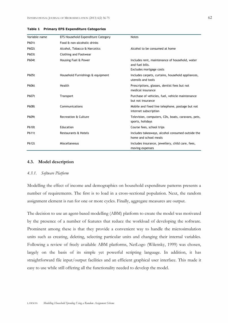
(COICOP) categories (UN, 2013). Table 1 provides a brief summary of each type and some
notes on what is included.
INTERNATIONAL JOURNAL OF MICROSIMULATION (2013) 6(2) 56-75 62
LAWSON Modelling Household Spending Using a Random Assignment Scheme
Table 1 Primary EFS Expenditure Categories
Variable name EFS Household Expenditure Category Notes
P601t Food & non-alcoholic drinks
P602t Alcohol, Tobacco & Narcotics Alcohol to be consumed at home
P603t Clothing and Footwear
P604t Housing Fuel & Power Includes rent, maintenance of household, water
and fuel bills.
Excludes mortgage costs
P605t Household Furnishings & equipment Includes carpets, curtains, household appliances,
utensils and tools
P606t Health Prescriptions, glasses, dentist fees but not
medical insurance
P607t Transport Purchase of vehicles, fuel, vehicle maintenance
but not insurance
P608t Communications Mobile and fixed line telephone, postage but not
internet subscription
P609t Recreation & Culture Television, computers, CDs, boats, caravans, pets,
sports, holidays
P610t Education Course fees, school trips
P611t Restaurants & Hotels Includes takeaways, alcohol consumed outside the
home and school meals
P612t Miscellaneous Includes insurance, jewellery, child care, fees,
moving expenses
4.3. Model description
4.3.1. Software Platform
Modelling the effect of income and demographics on household expenditure patterns presents a
number of requirements. The first is to load in a cross-sectional population. Next, the random
assignment element is run for one or more cycles. Finally, aggregate measures are output.
The decision to use an agent-based modelling (ABM) platform to create the model was motivated
by the presence of a number of features that reduce the workload of developing the software.
Prominent among these is that they provide a convenient way to handle the microsimulation
units such as creating, deleting, selecting particular units and changing their internal variables.
Following a review of freely available ABM platforms, NetLogo (Wilensky, 1999) was chosen,
largely on the basis of its simple yet powerful scripting language. In addition, it has
straightforward file input/output facilities and an efficient graphical user interface. This made it
easy to use while still offering all the functionality needed to develop the model.
INTERNATIONAL JOURNAL OF MICROSIMULATION (2013) 6(2) 56-75 63
LAWSON Modelling Household Spending Using a Random Assignment Scheme
4.3.2. Implementation
An overview of the program algorithm is shown below depicting the main stages of the
simulation.
load cross-sectional household data file from the EFS
for each simulated year
for each household
increase income by chosen percentage
for each household
locate a donor household that has a similar composition
and previous income, similar to the current household’s new
income
copy expenditure pattern from donor
calculate new aggregated expenditures for categories of interest
4.3.3. Matching criteria
One of the essential features of this algorithm is to locate a similar household. There are many
ways this can be done and the selection of which particular method to use will depend on the
application and available data. O’Hare (2000) describes several approaches for matching similar
cases. These include minimum distance matching, where the donor case is chosen due to its
closeness on one or more parameters. A common distance function is the normalised Euclidian
distance √∑(xi - yi)2 where xi and yi are the parameters for case i. This can be extended for as many
parameters as required. One of the advantages of minimum distance matching is that it can be
used on continuous data. If the data are categorical, matching can take place by random selection
of a donor case within the same class. These methods can be combined in matching by minimum
distance within classes. A further option that could be explored is to use cluster analysis to define
equivalence classes and select the donor case from within the appropriate cluster. In the
simulation described here, matching takes place using household income, the number of people

INTERNATIONAL JOURNAL OF MICROSIMULATION (2013) 6(2) 56-75 64
LAWSON Modelling Household Spending Using a Random Assignment Scheme
in the household and a derived variable known as household type. In O’Hare’s classification, this
is minimum distance within classes.
The essential feature of this model is that whenever a household experiences a change in income,
the expenditure pattern is copied from a similar household that has already had the new income
and has had time to adapt. As a result, income, by definition, will be one of the matching criteria.
It is represented as if it were a continuous variable so there are no income bands. In many cases,
there is not an exact match for a particular income so it is necessary to find the closest alternative.
In this implementation, for half of the cases (selected by a random draw), the household with the
next higher income is selected as the donor. In the other half, the next lower income household
is used. If more than one household satisfies the matching criteria, one of them is selected at
random.
Since incomes become more widely separated towards the top of the income distribution, there is
a possibility that in some cases, a small intended increase in income can lead to a large jump in
that copied from the next higher donor. To reduce this effect, a limit was put in place so that
donor incomes cannot be more than twice the intended percentage change in household income.
If there are no appropriate donors, all expenditures are changed in proportion to the desired
income change and no copying is done for that household in the current cycle.
Households have many characteristics apart from their income and expenditure pattern. One of
these is the number of people in the household and it is known that this is correlated with
household income (OECD, 2012). If the only matching criterion were income, then selected
donor households would be more likely to come from those that have a greater number of
occupants. Since households are unlikely to adapt to increasing incomes by taking in new
members, this effect was removed by including the number of occupants in the matching criteria.
Household income may also be correlated with the age and sex of occupants. This was controlled
for by classifying households by their composition. The following household types were defined
and each household was assigned to one of them.
Type Description Definition
1 One person non-pensioner one person below pensionable age
2 One person pensioner one person of pensionable age
3 Couple with no children two adults

INTERNATIONAL JOURNAL OF MICROSIMULATION (2013) 6(2) 56-75 65
LAWSON Modelling Household Spending Using a Random Assignment Scheme
4 Family with children two adults + 1 or more children
5 Single parent one adult + 1 or more children
6 Other all other households
(For the purposes of this model, an individual is considered to be an adult if they are aged 16 or over and a child if
under 16. Males aged 65 and over are considered pensionable as are females aged 60 or over.)
In order to simulate the effect of changing household incomes, a scenario is run where all
households receive a fixed percentage change in income. Processing continues until all
households have had their income changed or when the mean income of the population has been
changed by the target amount, whichever comes first. Details of the random assignment
procedure are shown below, beginning from the point where all households have been set a
desired or target percentage increase in income.
for each household
while mean population income <= target population income
select uniformly distributed random number from 0 to 1
if number <= 0.5 (copy from next higher income household)
if any other households with (income >= target) and (increase <= limit)
and same type and number in household
store donor expenditure pattern
else
change all spending categories in proportion to income change
if number > 0.5 (copy from next lower income household)
if any other households with (income <= target) and (increase <= limit)
and same type and number in household
store donor expenditure pattern
else

INTERNATIONAL JOURNAL OF MICROSIMULATION (2013) 6(2) 56-75 66
LAWSON Modelling Household Spending Using a Random Assignment Scheme
change all spending in proportion to income change
for each household
update expenditure patterns from stored donor
The source code and further details of the model can be found in the OpenABM model library
http://www.openabm.org/
4.3.4. Running the Model
In order to run a simulation, it is first necessary so set up some user defined parameters. These
are the number of cases to read from the input file, the number of cycles of random assignment
to run and the percentage change in real household income per cycle. It is possible to vary the
rate of income change to represent a particular scenario either via a slider on the user interface or
in the program code. The output appears in graphical form on the screen or optionally can be
written to a file for later analysis.
4.4. Results
4.4.1. The Average Household
When the initial data file, taken from the 2006 EFS, was read in, mean household income (before
tax and including any benefits) was £656. This was increased in a series of 10 steps (10 cycles of
random assignment) until it reached £1057, which represents a 61% increase. During this time,
mean total consumption expenditure rose from £478 to £654, which is an increase of 37%. This
is in agreement with the first two stylised facts, identified above, that expenditures rise with rising
income but at a slower rate. As mentioned earlier, the additional income goes partly on income
tax, some is saved or invested and some is spent on non-consumption items. This includes
mortgage interest payments, which appear in the EFS category ‘other expenditure’. In addition,
capital repayment of mortgage is not counted as consumption expenditure.
The output from the simulation takes the form of a cross-sectional population of households and
individuals within them. This is the same format as the original input file and enables a high level
of flexibility in the analysis of the results. The output can be written to a micro level data-file and
examined using a statistics package or represented graphically to highlight trends. The output
could also be used as input for further transformations of the population. For example, an
employment module could be added and expenditures copied from similar households that have
INTERNATIONAL JOURNAL OF MICROSIMULATION (2013) 6(2) 56-75 67
LAWSON Modelling Household Spending Using a Random Assignment Scheme
the same number of working and unemployed members. A demographic module could be set up
to represent the effect of population change with expenditure patterns copied from households
with a similar composition.
It would not be appropriate to write out the disaggregated output dataset here. The following
aggregated summary shows how the population reacts to increases in household income. This
can be compared against the stylised facts mentioned above to verify that the model produces the
expected results.
Table 2 shows expenditure changes for the average household. The ‘Initial Share’ is the
proportion of total consumption expenditure that the average household spent on each category
at the start of the simulation. The ‘Final Share’ is the budget share for the item after incomes
were inflated as described above. ‘Shift in Budget Share’ is the difference between the initial and
final share. Due to the stochastic nature of the simulation, there is some variation from one run
to the next. As a result, it is not possible to know whether the results from a single instance are
typical or unusual. Running the simulation a few times will provide information on how much
random variation takes place between runs. This can be quantified in a number of ways such as
calculating the difference between maximum and minimum values of the output for a particular
parameter, obtained from a number of runs or from their standard deviation. It is also possible to
calculate confidence intervals for the results and the next column of Table 2 gives the 95%
confidence interval of the final budget share for each expenditure category. The last two columns
of Table 2 show the upper and lower bounds of the confidence intervals. The results are the
mean of three simulations. The variation is assumed to be normally distributed because the
process generating the deviations is the random assignment scheme itself. While this gives some
indication of the variability of the model, it gives no indication of the accuracy of the model
specification.
Table 2 is sorted into descending order of percentage change so that as incomes rise, households
devote a greater proportion of their consumption expenditure to the goods near top of the list.
These categories can be said to have a greater discretionary element than those lower down.

INTERNATIONAL JOURNAL OF MICROSIMULATION (2013) 6(2) 56-75 68
LAWSON Modelling Household Spending Using a Random Assignment Scheme
Table 2 Share of Expenditure with Increasing Income (all households)
Expenditure
Category
Initial Share
(%)
Final Share
(%)
Shift in
Budget Share
(%)
95%
Confidence
Interval (+ -)
α = 0.05,
n = 3
Lower CI Upper CI
Transport 13.00 13.94 0.95 0.288 13.65 14.23
Education 1.48 2.31 0.82 0.242 2.07 2.55
Furniture 6.32 6.58 0.26 0.200 6.38 6.78
Miscellaneous 7.54 7.63 0.09 0.152 7.48 7.78
Health 1.24 1.31 0.07 0.033 1.28 1.34
Clothing 4.86 4.79 -0.08 0.095 4.70 4.89
Hotels 7.92 7.79 -0.13 0.007 7.78 7.80
Communication 2.46 2.1 -0.36 0.017 2.08 2.12
Recreation 12.26 11.89 -0.37 0.325 11.57 12.22
Alcohol 2.33 1.94 -0.39 0.039 1.90 1.98
Housing 9.94 8.92 -1.02 0.167 8.75 9.09
Food 9.81 8.14 -1.67 0.059 8.08 8.20
The expenditure shares to not add up to 100% because some spending goes to other items not included in these categories.
Table 2 indicates that the categories of ‘education’ and ‘transport’ receive a greater share of the
increased expenditure than the other items. This is consistent with the ONS results mentioned
above, which showed that households in the highest income decile spend more of their income
in these categories than those in the lowest income decile.
At the bottom end, ‘food’ and ‘housing’, receive a diminishing share of the rising income, which
is consistent with what was reported by the ONS. Finally, the budget share for ‘food’ falls as
incomes rise and this is in agreement with Engel’s Law.
These results are not surprising. They are merely intended to verify that the model produces the
expected results. However, the micro-level cross-sectional output can be analysed in a variety of
ways and the next section shows trends in more detail and later compares the results among sub-
sections of the population.
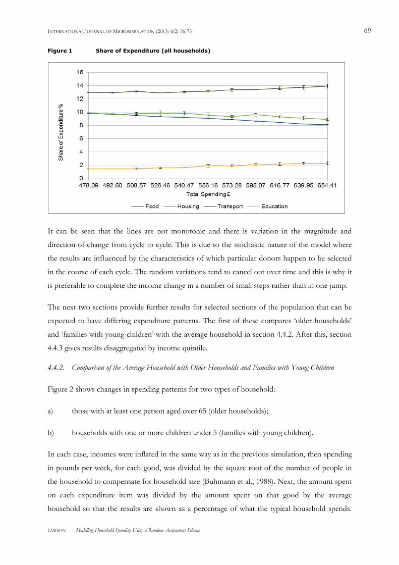
Figure 1 shows the results at regular points during the simulation. The share of consumption
expenditure is given as a percentage, on the y-axis. Only the top two and bottom two items from
Table 2 are plotted. This makes them easier to see and these are the items that exhibited the most
variation. The 95% confidence intervals are shown for each data point and indicate that random
variation is relatively small in this simulation.
INTERNATIONAL JOURNAL OF MICROSIMULATION (2013) 6(2) 56-75 69
LAWSON Modelling Household Spending Using a Random Assignment Scheme
Figure 1 Share of Expenditure (all households)
It can be seen that the lines are not monotonic and there is variation in the magnitude and
direction of change from cycle to cycle. This is due to the stochastic nature of the model where
the results are influenced by the characteristics of which particular donors happen to be selected
in the course of each cycle. The random variations tend to cancel out over time and this is why it
is preferable to complete the income change in a number of small steps rather than in one jump.
The next two sections provide further results for selected sections of the population that can be
expected to have differing expenditure patterns. The first of these compares ‘older households’
and ‘families with young children’ with the average household in section 4.4.2. After this, section
4.4.3 gives results disaggregated by income quintile.
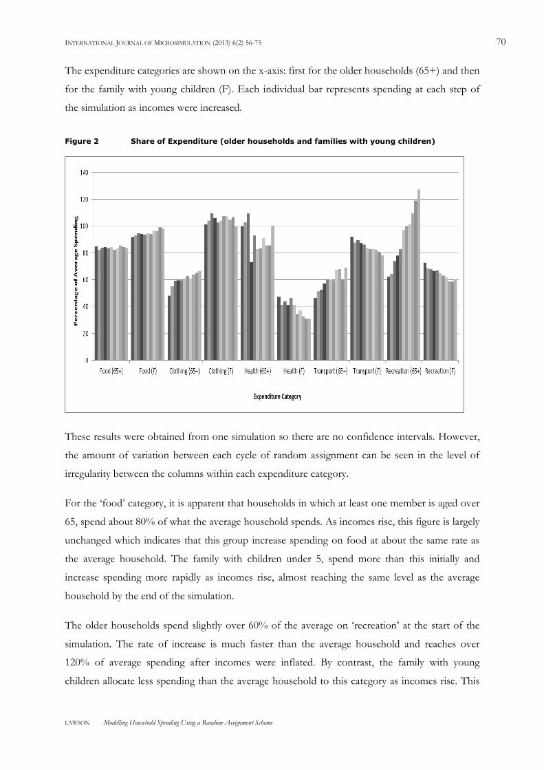
4.4.2. Comparison of the Average Household with Older Households and Families with Young Children
Figure 2 shows changes in spending patterns for two types of household:
a) those with at least one person aged over 65 (older households);
b) households with one or more children under 5 (families with young children).
In each case, incomes were inflated in the same way as in the previous simulation, then spending
in pounds per week, for each good, was divided by the square root of the number of people in
the household to compensate for household size (Buhmann et al., 1988). Next, the amount spent
on each expenditure item was divided by the amount spent on that good by the average
household so that the results are shown as a percentage of what the typical household spends.
INTERNATIONAL JOURNAL OF MICROSIMULATION (2013) 6(2) 56-75 70
LAWSON Modelling Household Spending Using a Random Assignment Scheme
The expenditure categories are shown on the x-axis: first for the older households (65+) and then
for the family with young children (F). Each individual bar represents spending at each step of
the simulation as incomes were increased.
Figure 2 Share of Expenditure (older households and families with young children)
These results were obtained from one simulation so there are no confidence intervals. However,
the amount of variation between each cycle of random assignment can be seen in the level of
irregularity between the columns within each expenditure category.
For the ‘food’ category, it is apparent that households in which at least one member is aged over
65, spend about 80% of what the average household spends. As incomes rise, this figure is largely
unchanged which indicates that this group increase spending on food at about the same rate as
the average household. The family with children under 5, spend more than this initially and
increase spending more rapidly as incomes rise, almost reaching the same level as the average
household by the end of the simulation.
The older households spend slightly over 60% of the average on ‘recreation’ at the start of the
simulation. The rate of increase is much faster than the average household and reaches over
120% of average spending after incomes were inflated. By contrast, the family with young
children allocate less spending than the average household to this category as incomes rise. This
INTERNATIONAL JOURNAL OF MICROSIMULATION (2013) 6(2) 56-75 71
LAWSON Modelling Household Spending Using a Random Assignment Scheme
leads to a decline in budget share for ‘recreation’ compared with the average household. In this
way, the graph gives an indication of the relative priority of allocating the extra spending due to
rising incomes.
4.4.3. Analysis by Household Income Quintile
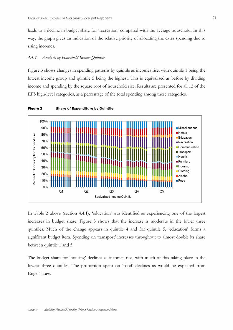
Figure 3 shows changes in spending patterns by quintile as incomes rise, with quintile 1 being the
lowest income group and quintile 5 being the highest. This is equivalised as before by dividing
income and spending by the square root of household size. Results are presented for all 12 of the
EFS high-level categories, as a percentage of the total spending among these categories.
Figure 3 Share of Expenditure by Quintile
In Table 2 above (section 4.4.1), ‘education’ was identified as experiencing one of the largest
increases in budget share. Figure 3 shows that the increase is moderate in the lower three
quintiles. Much of the change appears in quintile 4 and for quintile 5, ‘education’ forms a
significant budget item. Spending on ‘transport’ increases throughout to almost double its share
between quintile 1 and 5.
The budget share for ‘housing’ declines as incomes rise, with much of this taking place in the
lowest three quintiles. The proportion spent on ‘food’ declines as would be expected from
Engel’s Law.
INTERNATIONAL JOURNAL OF MICROSIMULATION (2013) 6(2) 56-75 72
LAWSON Modelling Household Spending Using a Random Assignment Scheme
5. DISCUSSION
This example shows how a random assignment scheme can be applied to model a set of several
goods at a disaggregated level. The matching scheme used here selects a donor case and from
there, any variables from the donor can be copied to the receiver. As a result, there is no
restriction on the number of goods that can be modelled. In principle, every item in the EFS
could be represented and the complexity of the model would rise linearly with the number of
goods. Also, since the individual households are retained, the distribution of variables is
preserved and output can be produced at the micro-level.
This does not mean the method is without pitfalls. As was mentioned above, selecting cases on a
parameter such as increasing income means that all the variables from the case will be available
for copying and some of these will be correlated with income. If the change in income really
causes the change in another variable, this can be used to determine the effect of the former on
the latter. However, if the change in income does not cause the change, such as when income
does not cause household size to increase, this will lead to an inaccurate estimation of the effect
because the simulated households change in a way that real households do not. This can be
minimised by including more variables in the matching criteria to limit the household’s response
to changing conditions. A sensitivity analysis can be done by adding matching criteria, one by
one, until the change in output reduces to an acceptable level. A regression of the matching
variables on the output variables will indicate how much of the variation is explained by the
model and so give an indication of its reliability. The problem of model specification is not
unique to random assignment and all modelling methods can be done well or badly whatever
approach is taken.
Although random assignment preserves the individual cases, the model described above does not
model trajectories. It is based on a cross-sectional dataset and assumes that households will
respond to a change in circumstances by adjusting their spending patterns to become more like
those that have already experienced the new conditions. This may have some plausibility but it is
also reasonable to suppose that households would try to retain as much of their original
behaviour as possible. It would be feasible to model this by using a longitudinal dataset and
copying from donors that have experienced a similar change over time. Unfortunately, the EFS is
a repeated cross-sectional survey and there are currently no large-scale longitudinal panel surveys,
in the UK at least, that monitor detailed household spending categories over time.
Random assignment is related to statistical matching, which is used in microsimulation to
INTERNATIONAL JOURNAL OF MICROSIMULATION (2013) 6(2) 56-75 73
LAWSON Modelling Household Spending Using a Random Assignment Scheme
combine data from a number of different sources or files. Here, individual cases are matched on
the basis of the similarity between one or more variables which are common to both sources
(Ingram et al., 2001). However, the random assignment scheme applied in this paper is essentially
different from statistical matching because records are matched from within the same dataset.
This makes it more akin to hot deck imputation where missing variables are obtained from a
similar case that has a complete set of variables (Andridge and Little, 2010). Hot deck imputation
is often used in surveys, where respondents may decline to answer some or all of the questions.
This is particularly problematic because different respondents may have different propensities for
omitting data so leading to biased results. A range of methods has been developed to ameliorate
this problem such as propensity score matching (Rosenbaum and Rubin, 1983) and multiple
imputation (Rubin, 1987). Here, the imputation process is repeated a number of times account
for the variability or uncertainty in the results, which is lost in a single imputation. This allows an
accurate statistical description of the resulting micro-level data file to be made. The model
described above also made use of multiple runs to average out the random element of the
imputation. This invites the possibility of combining the two approaches and further work in this
area may prove fruitful.
6. CONCLUSION
Modelling household expenditure is usually done by econometric methods but there are some
difficulties with this approach. These include the problem of modelling at a highly disaggregated
level and limits on the number of goods that can be represented. The example model described
in this paper shows that a random assignment scheme provides one way to avoid these
limitations. The paper set out to illustrate the practical advantages of random assignment and the
results point to areas for further research such as the possibility of matching using longitudinal
data and applying multiple imputation.
ACKNOWLEDGEMENTS
This research was supported financially by the UK Economic and Social Research Council
(ESRC) and BT plc. The work was supervised by Dr. Ben Anderson and I should like to thank
the anonymous reviewers for their insightful and constructive comments.
REFERENCES
Alpay S and Koc A (1998) ‘Household Demand in Turkey: An Application of Almost Ideal
INTERNATIONAL JOURNAL OF MICROSIMULATION (2013) 6(2) 56-75 74
LAWSON Modelling Household Spending Using a Random Assignment Scheme
Demand System with Spatial Cost Index’, Working Paper 0226, ERF Working Paper Series,
Economic Research Forum, Cairo.
Andridge R and Little R (2010) ‘A Review of Hot Deck Imputation for Survey Non-response’.
International Statistical Review, 78: 40–64. doi: 10.1111/j.1751-5823.2010.00103.x.
Buhmann B, Rainwater L, Schmaus G and Smeeding T (1988), ‘Equivalence Scales, Well-Being,
Inequality, and Poverty – Sensitivity estimates across 10 countries using the Luxembourg
Income Study (LIS), database’, Review of Income and Wealth, 115-142.
Deaton A and Muellbauer J (1980) ‘An Almost Ideal Demand System’, The American Economic
Review, Vol. 70, No 3, pp. 312-336.
Engel E (1857) Die Produktions und Consumtionsverhaltnisse des Kaonigreichs Sachsen,
reprinted with Engel (1895), Anlage 1, 1-54.
Engel E (1895) Das Lebenskosten belgischer Arbeiterfamilien frÄuher und jetzt, Bulletin de Institut
International de Statistique 9: 1-124.
Expenditure and Food Survey (2006) Economic and Social Data Service.
http://www.esds.ac.uk/findingData/snDescription.asp?sn=5986#doc
Holm E, Mäkilä K and Lundevaller E (2009) ‘Imitation or Interaction in Spatial Micro
Simulation’, Presentation at the 2nd General Conference of the International Microsimulation
Association, Ontario, Canada.
http://www.statcan.gc.ca/conferences/ima-aim2009/session3i-eng.htm#a44
Ingram D, O’Hare J, Scheuren F and Turek J (2001) ‘Statistical Matching: a new validation case
study’, Proceedings of the Section on Survey Research Methods, American Statistical Association, 746-751.
Klevmarken A, Andersson I, Brose P, Flood L, Olovsson P, and Tasiran A (1992) 'MICROHUS.
A Micro-simulation Model for the Swedish Household Sector. A Progress Report'. Paper
presented at the International Symposium on Economic Modelling, August 18-20,
Gothenburg, Sweden.
Klevmarken A and Olovsson P (1996) ‘Direct and behavioural effects of income tax changes -
simulations with the Swedish model MICROHUS’, in A. Harding (ed.), Micro-simulation and
Public Policy, Elsevier Science Publishers, Amsterdam.
INTERNATIONAL JOURNAL OF MICROSIMULATION (2013) 6(2) 56-75 75
LAWSON Modelling Household Spending Using a Random Assignment Scheme
Klevmarken A (1997) ‘Behavioural modelling in micro simulation models. A Survey’, Papers
1997-31, Uppsala – Working Paper Series.
OECD (2012) ‘What are Equivalence Classes’, OECD Project on Income Distribution and
Poverty, http://www.oecd.org/els/soc/OECD-Note-EquivalenceScales.pdf
O’Hare J (2000) 'Impute or Match? Strategies for Microsimulation Modelling', in Gupta, A. and
Kapur, V. (eds.), 2000 Microsimulation in Government Policy and Forecasting, Elsevier, London.
ONS (2008) Family Spending: 2007 Edition, Ed Dunn (Ed.), Palgrave MacMillan.
http://www.ons.gov.uk/ons/rel/family-spending/family-spending/2007-edition/index.html
ONS (2010) ‘Household Final Consumption Expenditure Summary’ 0.CN, Consumer Trends – Q2
2010, Office for National Statistics.
http://www.ons.gov.uk/ons/rel/consumer-trends/consumer-trends/q2-2010/index.html
Rosenbaum P and Rubin D (1983) ‘The Central Role of the Propensity Score in Observational
Studies for Causal Effects’, Biometrika, 70, pp. 41-50.
Rubin D (1987) Multiple Imputation for Nonresponse in Surveys, New York: John Wiley & Sons, Inc.
Thomas R (1987) Applied Demand Analysis, London, Longman.
UN (2013) United Nations Statistics Division, COICOP Detailed Structure and Explanatory
Notes. http://unstats.un.org/unsd/cr/registry/regcst.asp?Cl=5
Wilensky U (1999) NetLogo, http://ccl.northwestern.edu/netlogo/, Center for Connected
Learning and Computer-Based Modelling, Northwestern University, Evanston, IL.
Recommended