University of Wollongong University of Wollongong
Research Online Research Online
University of Wollongong Thesis Collection 1954-2016 University of Wollongong Thesis Collections
2016
Modelling and performance evaluation of net zero energy buildings Modelling and performance evaluation of net zero energy buildings
Joel Anderson University of Wollongong
Follow this and additional works at: https://ro.uow.edu.au/theses
University of Wollongong University of Wollongong
Copyright Warning Copyright Warning
You may print or download ONE copy of this document for the purpose of your own research or study. The University
does not authorise you to copy, communicate or otherwise make available electronically to any other person any
copyright material contained on this site.
You are reminded of the following: This work is copyright. Apart from any use permitted under the Copyright Act
1968, no part of this work may be reproduced by any process, nor may any other exclusive right be exercised,
without the permission of the author. Copyright owners are entitled to take legal action against persons who infringe
their copyright. A reproduction of material that is protected by copyright may be a copyright infringement. A court
may impose penalties and award damages in relation to offences and infringements relating to copyright material.
Higher penalties may apply, and higher damages may be awarded, for offences and infringements involving the
conversion of material into digital or electronic form.
Unless otherwise indicated, the views expressed in this thesis are those of the author and do not necessarily Unless otherwise indicated, the views expressed in this thesis are those of the author and do not necessarily
represent the views of the University of Wollongong. represent the views of the University of Wollongong.
Recommended Citation Recommended Citation Anderson, Joel, Modelling and performance evaluation of net zero energy buildings, Master of Philosophy thesis, School of Electrical, Computer and Telecommunications Engineering, University of Wollongong, 2016. https://ro.uow.edu.au/theses/4927
Research Online is the open access institutional repository for the University of Wollongong. For further information contact the UOW Library: [email protected]

MODELLING AND PERFORMANCE EVALUATION OF
NET ZERO ENERGY BUILDINGS
A thesis submitted in fulfilment of the requirements for the award of the
degree
Master of Philosophy
from
UNIVERSITY OF WOLLONGONG
By
Joel Anderson, B.E (Mechanical) (Hons)
School of Electrical, Computer, and Telecommunications
Engineering
2016


i
Declaration
I, Joel Anderson, declare that this thesis, submitted in fulfilment of the requirements for
the award of Master of Philosophy, in the School of Electrical, Computer, and
Telecommunications Engineering, University of Wollongong, is wholly my own work
unless otherwise referenced or acknowledged. The document has not been submitted for
qualifications at any other academic institution.
Joel Anderson

ii
Abstract
Developing a design philosophy to reduce carbon emissions from the built environment
is a major motivator for the formation of the net zero energy concept. For net zero
energy buildings to be widely adopted, a deeper understanding of the drivers of their
success is needed, as well as their comparative differences and similarities to buildings
of more conventional design. This thesis investigates the effects of different building
design and operation principles in relation to net zero energy buildings. Simulations of
three case study buildings (two of which are designed to be net zero energy) were
performed to identify the building design and operation elements which contribute most
to energy efficiency.
Through development and validation of building models of both net zero and
conventional designs in this thesis, it was found that validation of smaller, more energy
efficient building models can present challenges less commonly encountered in models
of more conventional buildings. An understanding of the sensitivities of net zero energy
buildings to alterations in design and specification were gained. Results show that net
zero energy buildings are more sensitive to changes such as glazing type, and HVAC
setpoint based on the case studies presented.
This thesis has looked at quantifying the contribution of different building elements and
systems to overall energy savings via simulation. The net impact of different glazing
types, lighting control methods, window shading schedules, and HVAC set points on
overall building energy consumption were examined.
This thesis also reports on the net zero energy balance for one case study building.
Results show that the building was net positive for the 12-month period considered.
Both energy imported/exported and energy generated/consumed were considered, as
well as the load matching, grid interaction, and some preliminary analysis of power
quality factors. These power quality factors and their relationship with net zero energy
buildings must be understood before the net zero concept can be widely adopted.

iii
Acknowledgements
This research has been conducted with the support of the Australian Government
Research Training Program Scholarship.

iv
Contents
Declaration ......................................................................................................................... i
Abstract ............................................................................................................................. ii
Acknowledgements .......................................................................................................... iii
Contents ........................................................................................................................... iv
List of tables ..................................................................................................................... ix
List of figures .................................................................................................................... x
List of abbreviations....................................................................................................... xiii
Chapter 1 Introduction ...................................................................................................... 1
1.1 Statement of the problem ................................................................................... 1
1.2 Research aim and objectives .............................................................................. 1
1.3 Research methodology ....................................................................................... 2
1.4 Publications related to this thesis ....................................................................... 3
1.5 Thesis structure................................................................................................... 3
Chapter 2 Literature Review ............................................................................................. 5
2.1 Background ........................................................................................................ 5
2.1.1 The growth of global energy consumption ................................................. 5
2.1.2 Impacts of climate change on the built environment .................................. 6
2.1.3 The need for net zero energy buildings ....................................................... 8
2.2 Net zero energy building definitions .................................................................. 8
2.3 Useful data and reporting methods ................................................................... 13
2.3.1 Balance metric ........................................................................................... 13
2.3.2 Balance period........................................................................................... 14
2.3.3 Type of balance ......................................................................................... 14
2.3.4 Measurement and verification ................................................................... 14
2.4 Certification schemes ....................................................................................... 18
2.4.1 Description of certification schemes ......................................................... 18

v
2.4.2 Comparison of certification schemes ........................................................ 21
2.5 Demand-side factors in net-zero energy buildings ........................................... 23
2.5.1 Energy efficiency ...................................................................................... 23
2.5.2 Occupant behaviour .................................................................................. 26
2.6 Supply-side factors in net-zero energy buildings ............................................. 29
2.6.1 On-site renewable generation .................................................................... 29
2.6.2 Load Matching and Grid Interaction ......................................................... 33
2.6.3 Off-site Renewable Generation ................................................................. 36
2.6.4 Distributed Generation & Microgrids ....................................................... 37
2.7 Building Performance Modelling Options ....................................................... 38
2.7.1 DOE-2 ....................................................................................................... 39
2.7.2 eQUEST .................................................................................................... 39
2.7.3 BLAST ...................................................................................................... 40
2.7.4 EnergyPlus ................................................................................................ 40
2.7.5 DesignBuilder ........................................................................................... 41
2.8 Summary .......................................................................................................... 41
Chapter 3 Methodology and Description of Case Studies .............................................. 44
3.1 Introduction ...................................................................................................... 44
3.2 Uncertainties in building energy modelling ..................................................... 44
3.2.1 Weather data in model validation ............................................................. 46
3.2.2 Model validation methodology ................................................................. 46
3.3 Simulation methodology .................................................................................. 49
3.3.1 Glazing ...................................................................................................... 51
3.3.2 Lighting ..................................................................................................... 52
3.3.3 Window Shading ....................................................................................... 54
3.3.4 HVAC ....................................................................................................... 55
3.4 Sustainable Buildings Research Centre – University of Wollongong.............. 56

vi
3.4.1 Building façade ......................................................................................... 57
3.4.2 Energy efficiency ...................................................................................... 58
3.4.3 Local generation ........................................................................................ 59
3.4.4 Description of Building Systems .............................................................. 59
3.4.5 Energy monitoring .................................................................................... 60
3.5 Transformational Technical Training Building – TAFE NSW ........................ 61
3.5.1 Building façade ......................................................................................... 62
3.5.2 Energy efficiency ...................................................................................... 62
3.5.3 Local generation ........................................................................................ 63
3.5.4 Description of Building Systems .............................................................. 63
3.5.5 Energy monitoring .................................................................................... 65
3.6 Enterprise 1 – University of Wollongong ........................................................ 65
3.6.1 Building façade ......................................................................................... 65
3.6.2 Energy efficiency ...................................................................................... 66
3.6.3 Description of building systems ................................................................ 67
3.6.4 Energy monitoring .................................................................................... 67
3.7 Summary of building features .......................................................................... 67
3.8 Summary .......................................................................................................... 68
Chapter 4 Model Validation & Performance Simulation................................................ 70
4.1 Purpose of building simulation......................................................................... 70
4.1.1 Relevance to net zero energy .................................................................... 70
4.2 Planned outcomes of simulations ..................................................................... 71
4.3 Background of models...................................................................................... 72
4.3.1 TTT ........................................................................................................... 72
4.3.2 SBRC ........................................................................................................ 75
4.3.3 Enterprise 1 ............................................................................................... 76
4.3.4 Summary ................................................................................................... 77

vii
4.4 Validation of models ........................................................................................ 77
4.4.1 TTT ........................................................................................................... 78
4.4.2 SBRC ........................................................................................................ 88
4.4.3 Enterprise 1 ............................................................................................... 99
4.4.4 Model limitations .................................................................................... 101
4.5 Summary ........................................................................................................ 102
Chapter 5 Simulation Results and Discussion .............................................................. 105
5.1 Simulation Results .......................................................................................... 105
5.1.1 Glazing .................................................................................................... 106
5.1.2 Lighting control ....................................................................................... 115
5.1.3 Window shading ..................................................................................... 118
5.1.4 HVAC setpoint ........................................................................................ 127
5.2 Summary ........................................................................................................ 131
Chapter 6 Energy Balance & Grid Interaction of Case Study Building ....................... 134
6.1 Considerations in the calculation of building energy balance ........................ 134
6.2 SBRC energy balance ..................................................................................... 136
6.2.1 NZEB – Site energy ................................................................................ 136
6.2.2 NZEB – Source energy ........................................................................... 138
6.3 Load-matching & grid interaction considerations for the SBRC ................... 143
6.3.1 Load match index .................................................................................... 143
6.3.2 Grid interaction index ............................................................................. 146
6.3.3 Power quality considerations of net zero energy buildings .................... 147
6.4 Summary ........................................................................................................ 149
Chapter 7 Conclusion and Future Work ....................................................................... 151
7.1 Building model validation .............................................................................. 151
7.2 Building simulation results ............................................................................. 152
7.3 Energy balance & grid considerations of case study NZEB .......................... 153

viii
7.4 Suggested future research ............................................................................... 154
Appendices .................................................................................................................... 157
References ..................................................................................................................... 162

ix
List of tables
Table 2-1 NZEB definitions and advantages/disadvantages from [11]. ......................... 10
Table 2-2 NZEB classification by [15]. .......................................................................... 12
Table 2-3 Results of energy rating comparison. From [27]. ........................................... 21
Table 2-4 Summary of physical modelling techniques from [66] .................................. 39
Table 3-1 Summary of building features ........................................................................ 68
Table 4-1 TTT representative zones for temperature validation. .................................... 79
Table 4-2 SBRC representative zones for temperature validation. ................................. 89
Table 4-3 SBRC model thermal validation periods. ....................................................... 89
Table 4-4 Building model thermal behaviour error summary. ..................................... 102
Table 4-5 Building model energy use error summary. ................................................. 103
Table 5-1 Glazing simulation scenarios. ....................................................................... 107
Table 5-2 Case study building envelope parameters..................................................... 108
Table 5-3 Building model lighting specifications. ........................................................ 115
Table 5-4 Shading simulation control strategies. .......................................................... 119
Table 5-5 HVAC setpoint simulation methodology. .................................................... 128
Table 5-6 HVAC setpoint simulation: building model HVAC details. ........................ 129
Table 6-1 Comparison of errors for imported/exported calculation methodologies. .... 141
Table B-1 Results from [28]. ........................................................................................ 158
Table B-2 Energy savings potential of different strategies by [38]. ............................. 159
Table C-3 List of available data related to this thesis ................................................... 160
x
List of figures
Figure 2-1 Angular relationship between the sun and a tilted flat plane [46]. ................ 30
Figure 2-2 Typical load/gen profile for residential building with solar PV - [55].......... 34
Figure 3-1 Model validation methodology. .................................................................... 47
Figure 3-2 Proposed building simulation methodology. ................................................. 50
Figure 3-3 Glazing simulation procedure. ...................................................................... 51
Figure 3-4 Lighting simulation procedure. ..................................................................... 53
Figure 3-5 Building model lighting schedules ................................................................ 53
Figure 3-6 Building model occupancy schedules ........................................................... 54
Figure 3-7 Window shading simulation procedure. ........................................................ 54
Figure 3-8 HVAC simulation procedure. ........................................................................ 55
Figure 3-9 Building model HVAC schedules ................................................................. 56
Figure 3-10 Sustainable Buildings Research Centre (SBRC). ........................................ 57
Figure 3-11 SBRC building façade section example [76]. ............................................. 58
Figure 3-12 Transformational Technical Training (TTT) building. ............................... 62
Figure 3-13 TTT building HVAC water services schematic [78]. ................................. 64
Figure 3-14 TTT building HVAC air services schematic [78]. ...................................... 64
Figure 3-15 TTT electrical meters and sub-meters. ........................................................ 65
Figure 3-16 Enterprise 1 building east/west timber louvres [79]. ................................... 66
Figure 4-1 TTT building model physical geometry as modelled in DesignBuilder. ...... 73
Figure 4-2 SBRC building model physical geometry as modelled in DesignBuilder. ... 75
Figure 4-3 Enterprise 1 model physical geometry as modelled in DesignBuilder. ........ 77
Figure 4-4 TTT Ground floor office temperature profile comparison. ........................... 79
Figure 4-5 R2 for ground floor office temperature comparison. ..................................... 80
Figure 4-6 TTT Seminar room temperature profile comparison. ................................... 81
Figure 4-7 TTT Building simulation room temperature profile comparison. ................. 82
Figure 4-8 R2 for building simulation room temperature comparison. ........................... 82
Figure 4-9 TTT gallery temperature profile comparison. ............................................... 83
Figure 4-10 TTT lighting electrical use comparison. ..................................................... 85
Figure 4-11 TTT equipment power electrical use comparison. ...................................... 86
Figure 4-12 TTT HVAC electrical use comparison. ....................................................... 87
Figure 4-13 SBRC energy lab temperature profile comparison – winter. ...................... 90
Figure 4-14 SBRC energy lab temperature profile comparison – summer. .................... 90

xi
Figure 4-15 R2 for energy lab room temperature comparison – summer. ...................... 91
Figure 4-16 SBRC water lab office temperature profile comparison – winter. .............. 92
Figure 4-17 R2 for water lab office room temperature comparison – winter. ................. 92
Figure 4-18 SBRC water lab office temperature profile comparison – summer. ........... 93
Figure 4-19 R2 for water lab office room temperature comparison – summer. .............. 93
Figure 4-20 SBRC eastern office temperature profile comparison – winter. ................. 94
Figure 4-21 R2 for eastern office room temperature comparison – winter. .................... 94
Figure 4-22 SBRC eastern office temperature profile comparison – summer. ............... 95
Figure 4-23 SBRC lighting electrical use comparison. ................................................... 96
Figure 4-24 SBRC IT electrical use comparison. ........................................................... 97
Figure 4-25 SBRC HVAC electrical use comparison. .................................................... 98
Figure 4-26 Enterprise 1 light and power electrical use comparison. ........................... 100
Figure 4-27 Enterprise 1 HVAC electrical use comparison. ......................................... 100
Figure 5-1 Energy Use Breakdown of three case study buildings. ............................... 105
Figure 5-2 Glazing simulations: change in HVAC energy use. .................................... 109
Figure 5-3 Glazing simulations: change in lighting energy use. ................................... 109
Figure 5-4 Glazing simulations: change in total building energy use. .......................... 110
Figure 5-5 Glazing simulations: change in HVAC energy use for identical LPD. ....... 111
Figure 5-6 Glazing simulations: change in lighting energy use for identical LPD. ...... 111
Figure 5-7 Glazing simulations: lighting system average weekly utilisation rates. ...... 113
Figure 5-8 TTT building level 1 floor plan [82]. .......................................................... 113
Figure 5-9 SBRC building level 1 floor plan [83]. ....................................................... 114
Figure 5-10 Lighting control simulations: yearly lighting energy use intensity. .......... 117
Figure 5-11 Lighting control simulations: yearly HVAC energy use intensity. ........... 117
Figure 5-12 Lighting control simulations: yearly building energy use intensity. ......... 118
Figure 5-13 Shading simulations: lighting energy use, seasonal schedule. .................. 120
Figure 5-14 Shading simulations: change in lighting energy/Awindow - seasonal. ......... 121
Figure 5-15 Shading simulations: HVAC energy - seasonal schedule. ........................ 122
Figure 5-16 Shading simulations: change in HVAC/Awindow - seasonal schedule. ....... 122
Figure 5-17 Shading simulations: lighting energy use - temperature control. .............. 123
Figure 5-18 Shading simulations: HVAC energy use - temperature control. ............... 124
Figure 5-19 Bellambi TMY weather file temperature histogram. ................................ 124
Figure 5-20 Occurrence of outside temperatures above 26°C. ..................................... 125
Figure 5-21 Shading simulations: building energy use - seasonal schedule. ................ 126

xii
Figure 5-22 Shading simulations: building energy use - temperature control. ............. 126
Figure 5-23 HVAC setpoint simulations: change in HVAC energy use. ..................... 130
Figure 5-24 HVAC setpoint simulations: change in building energy use. ................... 130
Figure 6-1 Australian electricity generation breakdown, 2012-13 [86]. ....................... 135
Figure 6-2 Australian energy flows, 2012-13[86]. ....................................................... 135
Figure 6-3 SBRC monthly site energy balance: 2015................................................... 137
Figure 6-4 SBRC cumulative site energy balance: 2015. ............................................. 137
Figure 6-5 PQA integral method definition. ................................................................. 139
Figure 6-6 Power profile comparison as measured by BMS & PQA: 5/07/2015. ........ 140
Figure 6-7 Comparison of imported/exported calculation methodologies. .................. 141
Figure 6-8 SBRC monthly source energy balance: 2015. ............................................. 142
Figure 6-9 SBRC cumulative source energy balance: 2015. ........................................ 142
Figure 6-10 SBRC net zero energy balance metric comparison: 2015. ........................ 143
Figure 6-11 SBRC average load and generation profiles: 2015. .................................. 144
Figure 6-12 SBRC 15-minute average power factor, real, and apparent power. ......... 147
Figure 6-13 SBRC THD of voltage and current on a typical day. ............................... 148
Figure 6-14 Maximum RMS voltage levels at the SBRC. ............................................ 149
Figure A-1 R2 for SBRC energy lab room temperature comparison - winter .............. 157
Figure A-2 R2 for SBRC Eastern Office temperature comparison - summer ............... 157
Figure B-3 NZEB balance for three definitions; Tracking of load/gen. - [17]. ............ 158

xiii
List of abbreviations
AHU Air Handling Unit
ASHP Air Source Heat Pump
BASIX Building Sustainability Index
BIPVT Building-Integrated Photovoltaic Thermal
BMS Building Management System
CASBEE Comprehensive Assessment System for Built Environment Efficiency
COP Coefficient of Performance
CVRMSE Coefficient of Variation of Root Mean Squared Error
DG Distributed Generation
DHW Domestic Hot Water
DSM Demand Side Management
E1 Enterprise 1
EE Energy Efficiency
EPBT Embodied Energy Payback Time
EUB Energy Use Breakdown
GBCA Green Building Council of Australia
GHG Green House Gas
GII Grid Interaction Index
GPO General Purpose Outlet
GSHP Ground Source Heat Pump
HVAC Heating Ventilation and Air Conditioning
IEA International Energy Agency
IEQ Indoor Environmental Quality
LBC Living Building Challenge
LEED Leadership in Energy and Environmental Design
LM Load Matching
LMI Load-Match Index
LowE Low Emissivity
LPD Lighting Power Density
lx Lux
NABERS National Australian Built Environment Rating Scheme

xiv
NMBE Normalised Mean Bias Error
NZE Net Zero Energy
NZEB Net Zero Energy Building
PEF Primary Energy Factor
PIR Photo Infrared
PQ Power Quality
PQA Power Quality Analyser
PV Photovoltaic
REC Renewable Energy Certificate/Credit
SBRC Sustainable Buildings Research Centre
SHGC Solar Heat Gain Coefficient
TAFE Technical And Further Education
THD Total Harmonic Distortion
THDI Total Harmonic Distortion – Current
THDV Total Harmonic Distortion – Voltage
TMY Typical Meteorological Year
TTT Transformational Technical Training building
UOW University Of Wollongong
VAV Variable Air Volume
VDI Virtual Desktop Infrastructure
WFR Window to Floor area Ratio
WWR Window to Wall area Ratio
1
Chapter 1 Introduction
1.1 Statement of the problem
With increasing average temperatures and more frequent extreme weather events as a
result of anthropogenic climate change, there is increased pressure on maintaining a
comfortable environment for building occupants while minimising building energy use.
In a study of the relationship between climate change, indoor thermal environment, and
building energy use, it was found that based on 2070 global warming predictions,
building energy use could be expected to rise by a range between 0.4% and 15.1%
depending on future climate scenarios and building location and design [1]. The studies
on Australian buildings predicted that temperate climates such as Sydney are likely to
be most sensitive to climate change, with cooling loads of buildings increasing by up to
101% [2].
The development of a new energy neutral, comfortable building design philosophy is
necessary to mitigate – and adapt to – the effects of climate change. Net zero energy
buildings are a way of meeting this new challenge.
Meeting the Net Zero Energy (NZE) requirements in Australian buildings is an
opportune area of research, with the goal of achieving net zero energy consumption
becoming more achievable due to the ongoing development of small scale solar and
wind technologies, and the emerging development of off-grid energy storage.
1.2 Research aim and objectives
The aim of this research is to evaluate the impact of existing building designs,
components, and operational parameters on fulfilling net zero energy requirements of
the University of Wollongong’s (UOW) Sustainable Buildings Research Centre (SBRC)
facility and Technical and Further Education TAFE Illawarra’s Transformational
Technical Training (TTT) building as part of the Living Building Challenge [3]. The
overall aim of the project is to address the following objectives:
1. Conducting a comprehensive literature review of current and past studies on the
building sustainability and net zero energy fields;
2. Development of building simulation models of the case study buildings using
DesignBuilder building performance simulation software for evaluating the

2
impact of building design, components and operational parameters on the overall
building energy use;
3. Validation of building models using real data collected from the case study
buildings;
4. Perform building simulations to evaluate the effectiveness of various designs
and operation strategies for each case study building and identify the most
effective ways of achieving net zero energy in a building;
5. Collect electricity consumption and generation data from case study buildings
and report on its progress in achieving net zero energy over its lifetime;
6. Report on load match and grid interaction factors, as well as basic power quality
considerations in net zero energy buildings through a case study building.
In addition to the two energy efficient case study buildings of the SBRC facility and
TTT building, an additional modern commercial building was also selected for
comparison against the net zero test cases.
1.3 Research methodology
In order to improve understanding of building operation and energy use, simulation
models of the case study buildings were developed in DesignBuilder. The 3D geometry
of each building comes from the as-built architectural drawings, while HVAC and
lighting specifications are sourced from the operation manual, as well as mechanical
and electrical drawings of the buildings.
Validation of the building models was carried out to ensure the models are appropriately
representative of the real buildings. To do this, historical weather data sourced from the
Bureau of Meteorology and the buildings’ own weather stations was coupled with
historical energy consumption and temperature data sourced from each building. By
performing benchmark simulations with the real weather data, the behaviour of the
simulated building was able to be compared to that of the real building with a common
weather input.
Once the benchmark model had been validated using historical weather data, it was then
modified according to different scenarios in order to determine the contribution of each
energy-saving technology to the overall performance of the building. The intended
3
outcome of these experiments was to understand some of the contributing factors to
energy efficiency in buildings.
The real weather data used for validation was sometimes not complete and/or not
always appropriate for the simulations. Accordingly, Typical Meteorological Year
(TMY) weather data was used. The reason for this is that TMY data is an amalgamation
of many years of weather data from the particular location in question, averaged out into
a year of representative data. This eliminates any extreme weather events and
unseasonable weather which may bias simulation results.
The collection of consumption and generation data for the test cases was mainly sourced
via the Building Management Systems (BMS) of the respective buildings’. The SBRC
BMS has a comprehensive data trending ability and electrical metering is available
down to a high level of detail for both loads and generators.
1.4 Publications related to this thesis
• J. Anderson, D. A. Robinson, and Z. Ma, “Energy Analysis of Net Zero Energy
Buildings: A Case Study,” in 12th REHVA World Congress CLIMA 2016,
2016.
Accepted for publication, and presented in May, 2016.
1.5 Thesis structure
The current chapter outlines the aims and objectives of this thesis. It presents the key
research methodologies employed. The subsequent chapters are organised as follows:
• Chapter 2 presents a comprehensive review of the literature relating to net
zero energy buildings;
• Chapter 3 gives a description of the buildings used as case studies in this
thesis as well as the building simulation and model validation
methodologies.

4
• Chapter 4 provides background of the development of each case study
building model and the planned outcomes of the simulations. The validation
process of each model is documented including quantification of associated
errors.
• Chapter 5 presents the results of the building simulations on each test case
and discusses the results and their implications for NZEBs.
• Chapter 6 is a presentation of the energy balance of a case study building
based on measured energy consumption and generation data. An analysis of
the load matching and grid interaction factors of the case study building, as
well as some power quality factors and implications of these for the utility
grid is carried out.
• Chapter 7 details the conclusions that can be drawn from research presented
in this thesis and outlines the potential for future work in this field.

5
Chapter 2 Literature Review
2.1 Background
The exponential growth, both in terms of economy and population throughout the
world, especially in developing countries, has resulted in dramatic increases in global
primary energy consumption. The demand for energy in recent decades has been met
overwhelmingly by fossil fuel resources. A side-effect of this is the onset of significant
climate change that will affect life on planet Earth for all living species.
For the human race, significant climate change means that urgent changes need to be
made to the way we live, and where we live, with increased pressures on our built
environment coming over time from a warming climate and more extreme weather
events. These changes give rise to the need for us to change the way our built
environment works; our building designs and codes, our energy consumption, how we
source our energy, as well as our own personal behaviour and living habits.
A focus on energy efficiency in our buildings is needed. Building performance
certification schemes are promising ways of ensuring buildings deliver meaningful
energy reduction in a structured and certified way. To enable effective implementation
of these performance targets, consistent methodologies need to be developed to ensure
reliable verification is able to take place. In addition to energy efficiency measures, it is
important that buildings are able to offset the reduced amount of energy that they
consume. On-site renewable generation is the best way of achieving this through
rooftop solar in most cases, though other methods such as the purchase of Renewable
Energy Certificates (REC) are also feasible for buildings where on-site renewable
generation is not possible.
2.1.1 The growth of global energy consumption
In their review of the sustainable development implications of zero energy buildings, Li
et al. [4] noted that during the rapid growth of the Chinese economy over the past few
decades, primary energy consumption increased from 0.57 billion tonnes of oil-
equivalent in 1978 to 3.25 billion tonnes in 2010 – growth of 470% and overtaking the
US as the world’s largest energy producer in 2009.
Through review of building energy consumption information, Pérez-Lombard et al. [5]
observed that global primary energy consumption grew by 49% between 1984 and

6
2004, attributing this to the rapid growth of developing economies and their resulting
improved living conditions. They concluded that current energy and socio-economic
systems are unsustainable.
Global energy demand is predicted to continue its growth trajectory onwards to 2035
according the International Energy Agency (IEA) in their World Energy Outlook report
for 2013 [6]. The report noted however that government policies during this time will
likely have significant impact on the consumption trend. The IEA’s ‘new policies’
scenario forecasted that all sources of energy will continue to grow during the period to
2035, but that renewable energy will grow by the greatest margin of 77% worldwide.
The consequence of this increased energy demand is that CO2 emissions are predicted to
increase by 20%.
2.1.2 Impacts of climate change on the built environment
With increased average temperatures as a result of anthropogenic climate change, there
is an increased pressure on our buildings to maintain a comfortable environment for
occupants. In a study of the relationship among climate change, the indoor thermal
environment and building energy use, Guan [1] found that building energy use could be
expected to rise by 0.4-15.1% depending on future climate scenarios and building
location and design, based on global warming predictions to the year 2070. Various
adaptation strategies were examined and it was suggested that the required heating and
cooling loads, and ultimately the overall energy use, could be reduced if the internal
load density of the building was reduced. These internal loads were defined as those
loads which generate heat and come from within the building envelope (e.g lighting and
plug loads). Further research into a ranking system of the viability of different
mitigation and adaptation strategies was suggested to enable optimising retrofit and
design projects.
A similar study into the relationship between buildings and climate change was
performed by de Wilde and Coley [7]. The authors warned that existing rules and
regulations in the building sector are based on historical climate data and are therefore
not necessarily well suited to the future in a warmer climate. They also suggested that
existing performance metrics should be considered carefully to account for human
perception of thermal comfort and their adaptation to wider temperature bands.
Performance metrics are methods by which the success and performance of a building is

7
measured over a variety of categories such as energy consumption or thermal comfort
surveys.
The potential impact of climate change on the energy requirements associated with
heating and cooling in five residential buildings throughout Australia was examined by
Wang et al. [2]. A major finding was that a significant impact on the heating and
cooling energy requirements may occur within the lifetime of the existing building
stock – highlighting that more research is required on retrofitting to mitigate these
potential impacts. Depending on the climate zone in which the building is situated, it
was predicted that by 2050, the total heating/cooling requirements of a newly
constructed 5-star house (NABERS rating) would vary within the range of -26% (where
the warming climate would reduce the heating load of a building in a location with a
traditionally high heating requirement) to 101% for more cooling dominated climates.
Temperate climates such as Sydney, where heating and cooling loads are relatively
balanced, are likely to be most sensitive to climate change, although Wang et al. [2]
noted that further studies are needed to investigate the implications of different types
and sizes of buildings. In addition, the thermostat settings used in this analysis were
those specified in current Australian building codes and did not consider the future
alterations of these codes, or future occupant behavioural adaptation.
Simulations were performed by Ren et al. [8] on existing and new residential buildings
in eight varying climate zones throughout Australia and identified potential adaptation
pathways to mitigate the effects of climate change and maintain current cooling/heating
energy requirements. It was concluded that a good level of adaptive capacity was
possible through energy efficiency measures for heating dominated buildings. For
cooling dominated buildings, additional measures are needed such as renewable energy
to offset the energy required by the larger cooling load.
Climate change’s impact on the built environment will manifest itself through increased
energy use due to the increased HVAC capacity required to cope with a warming
outside climate. It is clear that building codes must be updated to address the future
impacts on the built environment from climate change. The introduction of energy
efficiency measures and renewable energy resources make it possible for buildings to
adapt to these changes, maintaining a comfortable environment for occupants, whilst
dramatically reducing the energy required.

8
2.1.3 The need for net zero energy buildings
To mitigate the impact of climate change on the built environment, it is necessary to
develop a new design philosophy for our buildings that enable occupants to remain
comfortable in a warming climate, as well as reduce the environmental footprint and
emissions intensity of our structures.
Wilkinson et al. [9] argued that by decarbonising the built environment through
strategic changes to the way we use building elements such as insulation, ventilation,
fuel switching, and behavioural change, there is potential to prevent 5500 premature
indoor environment related deaths every year, as well as save 41 Mt of CO2 emissions.
Whilst there may be many benefits to rethinking how we design our built environment,
Pérez-Lombard et al. [5] suggested that it will be business as usual despite an increased
emphasis on energy efficiency minimum requirements, unless regulation steps in to
both raise social awareness of sustainability issues, and to enable new technologies for
energy production and energy conservation to enter the market.
In a review of the current status and future potential of the building sector in the UK,
Clarke et al. [10] highlighted the fact that many buildings have very poor energy
performance due to being constructed before building energy standards were developed.
This, combined with increases in electrical energy use, leads to the potential for
significant improvements in the efficiency of current building stock. The need for
upskilling in the industry to cope with new building technologies is identified by the
authors.
The proliferation of low energy intensive buildings which meet their own energy needs
through renewable means has great potential to minimise the effects of climate change,
and provide many public health benefits as a result. Whilst some regulation and industry
training incentives may be required to encourage the take-up of such changes, there is
huge potential in retrofitting existing building stock to minimise and perhaps eliminate
their net energy use.
2.2 Net zero energy building definitions
In principle, the concept of a Net zero Energy Building (NZEB) is relatively simple – a
building that produces at least as much energy as it consumes. However there are many

9
potential ways to define the ‘zero’ balance. Depending on the objective of the building
in question, and the regulatory environment in its jurisdiction, the specific definition of
‘net zero’ may vary.
Torcellini & Pless [11] studied four of the more common definitions in the literature
and discussed their applications, advantages, and disadvantages. They stated that a good
NZEB definition must first prioritise energy efficiency over renewable energy capacity.
A reduced load will lead to reduced required installed capacity of renewable energy,
leading to significant cost savings and making the NZEB goal more achievable.
The definitions studied in Torcellini & Pless [11] use the utility grid as a means of
accounting for net use. The four definitions discussed are net-zero site, net-zero source,
net-zero costs, and net-zero emissions:
• Net zero site – a NZEB that produces at least as much energy on site, as it
consumes in a year, accounted for at the site;
• Net zero source – a NZEB that produces at least as much energy as it uses in
a year, accounted for at the source. Source energy considers the primary
energy used to generate and transport the energy to the site. This is important
when accounting for energy consumed from the grid, where a significant
portion of energy is lost during transmission from generator to site, and in
thermal generation efficiency losses;
• Net zero cost – this balances the costs rather than the units of energy. So the
amount of money paid to the building owners/tenants by the utility for the
energy it exports, is at least equal to the amount spent by the building
owners/tenants for energy imported from the grid;
• Net zero emissions – again, a different metric is used to define the balance:
this time, emissions. The building produces at least as much emission-free
energy to offset the emissions intensive energy imported from the grid. Here,
non-energy differences between fuels such as carbon emissions, and other
types of pollution are accounted for. This makes it a more comprehensive
definition than the others but as a result, it is more difficult to implement.
The authors argued that the definition influences the design of the building and vice
versa. Depending on the definition, the emphasis can be placed on energy efficiency,
energy supply strategies, or a number of other factors which in turn influence practical

10
aspects of the building’s design and operation. Table 2-1 summarises the advantages
and disadvantages of the four definitions discussed.
Table 2-1 NZEB definitions and advantages/disadvantages from [11].
In a similar fashion to Torcellini & Pless [11], the understanding of a lack of consistent
international definition of NZEB was addressed by Sartori et al. [12]. It was recognised
that different definitions were possible to describe NZEBs depending on their purpose
and regulatory targets. A framework by which to set definitions was proposed according
to 5 criteria as described below and a methodology around this was developed to enable
setting of NZEB definitions in a systematic way. The NZEB framework criteria is a
refined version of Sartori et al. [13] and is organised as follows:
1. Building system boundary – energy flows that cross the defined system
boundary are considered in the NZEB analysis. Those energy flows that
don’t, are disregarded;
11
2. Weighting System – the weighting of different energy sources allows the
comparison of different sources throughout the energy chain on a normalised
basis. This allows for comparison of factors such as site and source energy,
and fuel switching (e.g. PV generation in summer, biomass generators in
winter), as well as cost and emissions metrics where there are differences
between energy sources in terms of generation and transmission costs, and
emissions per unit of energy supplied;
3. NZEB Balance – a number of factors influence the outcome of the NZEB
balance such as the time period over which the balance is calculated, the type
of balance, and whether there are minimum energy efficiency requirements
that must be met before NZEB status can be achieved. The balance period is
typically taken to be a year, as this will account for seasonal cycles. A
building that may not produce enough energy in winter may still generate a
large surplus in summer from its PV system and as such compensates for the
winter deficit. Some argue that a longer period closer to the building’s total
lifespan should be taken to account for the embodied energy of the building.
However it is possible to annualise the contribution of the embodied energy
so that this can still be considered using an annual balance period. The type
of balance has a significant influence on the achievability of the NZEB goal;
4. Temporal Energy Match Characteristics – in addition to a NZEB being able
to achieve balance over the balance period, there are other factors to be
addressed concerning the building’s interaction with the grid, as well as its
potential to produce enough energy at times of peak consumption;
5. Measurement and Verification – in order to check that the building is
complying with NZEB requirements, the authors argue that a proper
measurement and verification process be put in place. This process would be
dependent on the rest of the criteria discussed previously. It is argued that a
measurement and verification process should at least keep track of the
energy import/export balance, but it is recommended that further detail such
as temporal load characteristics be considered, as well as occupant comfort.
Two key challenges have been identified by Marszal et al. [14] that require attention
before the proper integration of NZEBs into national and international building codes
can occur. These include the need to adapt a common and unambiguous definition, and
to determine a standard methodology for calculating the energy balance. The metric of

12
the energy balance is recognised as being the most important point to address. The
authors state that while the delivered energy metric is the most easy to implement, it
does not account for primary energy losses and different types of energy. As such, the
primary energy metric is recommended.
A classification system based around the type of renewable energy resource use was
created by Pless & Torcellini [15]. The system ranges from NZEB:A to NZEB:D as
shown in Table 2-2. NZEB:A is a building that offsets all of its energy use from the
renewable energy available within the building footprint, whilst NZEB:D is a building
that achieves balance through a combination of on-site renewable energy and the
purchasing of renewable energy credits from an outside source. The aim of this
classification system is to encourage designers to first implement significant energy
efficiency measures before sizing an appropriate renewable energy system in order to
keep required capacity down as much as possible.
Table 2-2 NZEB classification by [15].
A summary of findings by Griffith et al. [16] from research conducted at the American
National Renewable Energy Laboratory concluded that the net zero site definition was
preferred for analysis due to ease of verification and does not require conversion factors.
However as discussed previously, this does not provide the most comprehensive
account of the overall energy balance of the building.

13
2.3 Useful data and reporting methods
In order to ensure the NZEB goal is achieved and maintained through the life of the
building it is important that data is easily obtained and shown through a sound
methodology, whether balance is achievable or not. A number of parameters need to be
defined depending on the type of NZEB building in question, and suitable reporting
methods must also be developed.
In a review of definitions and calculation methodologies by Marszal et al. [14], it is
argued that before a consistent definition can be developed, a number of factors need to
first be considered:
• The metric of the energy balance
• Balance period
• Type of energy to be included in balance
• Type of energy balance
• Accepted renewable energy supply options
• Grid connection
• Energy efficiency requirements
The study showed that these factors were of particular importance for designers and
operators. Possible solutions for the implementation of the above factors were discussed
however no recommendations were proposed. Rather, the aim was to give an overall
understanding of the various considerations in NZEB design and definition.
2.3.1 Balance metric
There are a number of different possible metrics used to define ‘zero’. Marszal et al.
[14] considered these metrics and found that the most favoured metric is primary energy
because this is quite comprehensive, considering different kinds of energy, as well as
the transmission losses from the grid. However the consideration of different kinds of
energy becomes complicated due to the underestimation of renewable energy resources.
For example, it requires 2-3 units of primary energy to produce 1 unit of delivered
energy from coal, while renewable energy sources require 1 unit of primary energy to
deliver 1 unit of energy. This means that a suitable conversion factor needs to be
adopted. However this factor is not static, as the percentage of renewable energy
penetration in the utility grid changes over time.

14
As well as the primary energy metric, the authors discuss the relevance of using CO2
emissions as the balance metric, given the global focus on emissions reduction.
However the point was made that buildings are commonly evaluated on their energy
performance as specified by building codes, rather than their emissions performance
which would make implementation of this metric difficult.
2.3.2 Balance period
The period of balance can have an impact on the achievability of the goal given the
seasonal variability of renewable energy resources. Sartori et al. [12] argued that a
yearly balance covering all seasonal conditions is most suitable. Longer periods in the
order of decades may be selected to account for embodied energy; however it is possible
to annualise this contribution to retain a yearly balance period. These findings are
generally in keeping with those found by Marszal et al. [14].
2.3.3 Type of balance
Marszal et al. [14] argued that for a grid connected NZEB, there are two possible types
of balance: energy use/renewable generation, and energy delivered from grid/energy fed
into grid. It was stated that energy use/renewable energy generated is more applicable
for the design phase of a building while the delivered/exported balance should be used
in operational monitoring. Despite this, it was concluded that the most popular balance
in the literature at the time was energy use/renewable energy generated. Sartori et al.
[12] concurs with the study by Marszal et al. [14].
2.3.4 Measurement and verification
To ensure proper compliance with the applied NZEB definition, a comprehensive
measurement and verification methodology should be implemented. Sartori et al. [12]
argued that as a bare minimum, this methodology should assess the energy
import/export balance, but that it would be beneficial to go further and assess the
temporal load match and grid interaction characteristics, as well as occupant comfort
and Indoor Environmental Quality (IEQ).
A Microsoft Excel based tool was developed by Belleri et al. [17] which assessed the
balance, operating costs, and load match index for NZEBs base on a set of pre-defined
definitions. It is suitable for designers, managers and policy makers in gauging the
potential success of an NZEB, as well as monitoring the building during operation.

15
The pre-defined definitions are decided by the tool through user input of a number of
parameters. The monthly or yearly energy supply/demand is able to be entered, and
desired weighting factors specified. The analysis period can be either yearly or monthly
and a number of different metrics are able to be chosen. The authors performed a case
study on a planned office building in Italy. The use of the tool enabled designers to
assess the predicted success of the building according to different definitions of NZEB.
A standardised monitoring and verification procedure was developed by Noris et al.
[18] to assist in planning, installation, and operation. They noted that several common
strategies already exist:
• Whole building approach – measures energy flow to/from entire building;
• Sub-metering approach – measurements of isolated energy uses are carried out;
• Indoor comfort – comfort parameters are measured to assess occupant comfort
and identify any system malfunctions.
The steps to be considered in the three phases of NZEB monitoring as proposed by
Noris et al [18] are summarised below:
Planning:
• Set monitoring objective and goals – determine any desired indices such as load
match and heating demand as well as IEQ;
• Collect building data – consider the energy flow present throughout the building
according to a standard format;
• Identify monitoring boundaries – these boundaries depend very much on the
definition being used and it is important that these are identified early and are
consistent with the definition chosen;
• Select metrics – different levels of monitoring may be considered based on the
monitoring goals chosen. It is stated that the minimum requirement is to obtain
the data required for balance verification. But further information regarding IEQ
and the delivered/exported balance would be beneficial;
• Perform data reduction – if possible, dependent metrics should be evaluated
according to their relationships to independent metrics. This ensures the size of
the data required is diminished, saving monitoring costs. This strategy can

16
reduce data reliability so close attention should be paid to the implications of
this strategy specific to each case;
• Define data collection frequency and duration – this factor depends highly on
the balance period selected in most cases. Monthly data is adequate for most
cases such as energy balance, however higher resolution data in the order of
hourly or sub-hourly is beneficial for the monitoring of load match and grid
interaction characteristics;
• Identify suitable sensors and data acquisition – with the necessary metrics
having been defined and the required data needed to assess them, it is possible
now to identify the specific sensors needed to measure the data. Factors such as
measurement duration, sample rate and desired accuracy must be considered.
Installing:
• Assess technical feasibility – it must be verified whether the selected equipment
is able to be installed in the building satisfactorily;
• Recognise and solve metering gaps – proper measures should be identified to
overcome any technical issues that result from the technical feasibility
assessment. This step must also consider the possible implications for the data
quality;
• Final plan and install;
• Commissioning – all components of the monitoring system must be set up to
give accurate and reliable service and tested extensively. This is a complex but
necessary task.
Operation:
• Define data quality assurance procedures – it is necessary to define quality
assurance protocols during operation for all data acquired and develop
contingencies for when data may be missing due to instrument breakdown, as an
example. In this case, an estimation procedure based on historical data may be
necessary;
• Post processing – raw data must be processed to calculate the balance and other
indicators of building performance. A standard procedure for this step should be
developed to ensure consistency through the life of the building;

17
• Reporting – a report will need to be delivered at the end of each balance period.
The authors of [18] recommend that a standard reporting procedure be
developed that contains the following three sections:
▪ A description of the building and its monitoring system including design
data and monitoring system specification. This section remains static and
constant throughout all reports in most cases, unless upgrades or
modifications are performed
▪ The results of the current year with easy to understand standardised
diagrams and explanations of the results (climate conditions, occupancy
rates etc.)
▪ Elaboration on all the data in the second section, and of observed trends
throughout previous reports.
• Planning and implementation of operational maintenance – this is needed to
ensure the monitoring system works consistently across all balance periods and
remains accurate and reliable. Maintenance activities should be planned at
appropriate intervals to check instrument calibration and data storage integrity.
A report by Marszal & Bourrelle [19] aimed to understand the differing approaches that
currently exist to calculate the energy balance of NZEBs. The importance of variable
selection is highlighted and the gap between the suggested methodology and European
building codes is examined to highlight the areas that need improvement in building
codes to bring them up to the standard of NZEB requirements. The most favoured
methodology was found to be the balance between energy use and renewable energy
generation. However, the ambiguity of ‘energy use’ shows that further definition is
needed to refine what is meant (calculated energy demand or actual measured
consumption). As well as this, the type of energy used in the analysis must also be
specified.
Measurement and verification tools and methodologies are essential in ensuring energy
flows within a building can be accounted for and comprehensively documented in order
to ensure NZEB status is attained and maintained. The data required must be identified
and obtained through the installation of suitable instrumentation. Depending on the
definition of NZEB that is being used, decisions must be made on the type of metric, the
period of balance, and types of energy to be included in the balance.

18
2.4 Certification schemes
A number of organisations, both government and non-government, have responded to
the increased awareness of building sustainability by developing codes, standards, and
rating systems designed around a framework of sustainability factors such as energy
use, water use, and building materials. These schemes are designed to assist owners,
designers, builders, and managers in developing their buildings according to an
established standard. A few of the main certification schemes that are in operation
worldwide are discussed below.
2.4.1 Description of certification schemes
2.4.1.1 BREEAM
The Building Research Establishment Environmental Assessment Methodology
(BREEAM) has been operating since 1990 and is widely considered to be the world’s
most popular scheme [20]. BREEAM was developed by the Building Research
Establishment (BRE). It enables developers, designers, and building managers to
improve the environmental performance of their buildings through a rating system that
considers energy and water use, occupant health, pollution, transport implications,
building materials, and building waste, as well as the environmental ecology impacts
and building management processes [21].
BREEAM claims to be the most widely used scheme in the UK and also operates in
several other countries including Germany, The Netherlands, Norway, Spain, Sweden,
and Austria. Several variations of the BREEAM scheme exist depending on the
regulatory environment of the country in which it operates, as well as the type of
building and its use (new or existing construction, community or stand-alone building,
residential or commercial)[22].
2.4.1.2 LEED
Leadership in Energy and Environmental Design (LEED) is a certification scheme
developed by the US Green Building Council (USGBC) that considers the design,
construction, operation, and maintenance of green buildings. Similar to the BREEAM
system, LEED is flexible to different project development and delivery processes by
having different rating systems depending on the type of project being considered.
LEED’s five rating system groups include Building Design and Construction; Interior

19
Design and Construction; Building Operations and Maintenance; Neighbourhood
Development; and Homes [23].
2.4.1.3 NABERS
The National Australian Built Environment Rating System (NABERS) provides a
comparison of the environmental performance of different Australian buildings. The
energy efficiency, water use, waste management, IEQ, and environmental impacts are
measured and a ‘Star’ rating is applied to show relative operational performance
compared to pre-defined benchmarks [24].
Rating system
As with the previous certification schemes discussed, the NABERS scheme includes
slightly different versions of the tools for the specific project being considered. There
are different variations of the tool for offices, hotels, shopping centres, data centres, and
homes. Twelve months of measured performance data is used to come up with a star
rating from zero to six. The measured performance data includes usage figures for
aspects such as electricity, gas, and water. Performance is compared to building
benchmarks that represent the performance of nearby buildings of a similar design.
In order to ensure performance data is comparable to the benchmarks, adjustment
factors may be used to account for the buildings climatic conditions, occupancy hours,
level of amenities, energy sources, and size. The star rating awarded is an indication of
its relative performance to the defined benchmark. It is not an indication of absolute
building performance, but rather a measure of how it compares to what is considered to
be the current standard.
2.4.1.4 Green Star
Green Star is a voluntary scheme launched by the Green Building Council of Australia
(GBCA) in 2003. It offers a “framework of best practice benchmarks for sustainability”
for building owners, operators, and occupants [25]. The key objectives of Green Star are
“to drive the transition of Australia’s property industry towards sustainability by
promoting green building programs, technologies, design practices and operations as
well as the integration of green building initiatives into the mainstream design,
construction and operation of buildings and communities” [26].

20
A number of different rating tools are available under the Green Star banner for
different building types. These are Design and As-Built, Interiors, Communities, and
Performance. The rating tools assess performance based on the following categories:
• Management
• Indoor Environment Quality
• Energy
• Transport
• Water
• Materials
• Land Use & Ecology
• Emissions
• Innovation
These categories are then quantified by being divided into credits in order to award
points when a particular aspect of improvement is achieved.
Green Star and net zero energy
Whilst there is no requirement in the Green Star process that buildings must be net zero,
and net zero energy or carbon neutrality is not specifically rewarded, the achievement of
net zero has substantial benefits for the standard certification process in the categories
of operating emissions and energy use.
2.4.1.5 Living Building Challenge
The Living Building Challenge is an initiative of the Living Future Institute to advocate
for the highest level of building sustainability. It promotes itself as a philosophy before
a certification program. The mission of the Living Building Challenge is “To encourage
the creation of Living Buildings, Landscapes and Communities in countries around the
world while inspiring, educating and motivating a global audience about the need for
fundamental and transformative change” [3]. The challenge exists in three ‘typologies’;
Buildings, Renovations, and Landscape & Infrastructure. Seven categories make up the
challenge, and these categories are further broken down into 20 imperatives. In order to
achieve Living Building status, it is necessary to accomplish all requirements of each
applicable imperative (this means all 20 for buildings, 15 for renovations, and 17 for
landscape and infrastructure).

21
Of relevance to this project, the energy under version 3.0 of the LBC requires net-
positive energy. This implies a surplus of energy is required with 105% of the
buildings’ energy needs to be met by on-site renewables. As well as this, on site storage
is also required as part of a focus on resiliency. At least 10% of lighting load and
refrigeration is required to be met for a minimum of one week by back up battery
storage.
2.4.2 Comparison of certification schemes
Roderick et al. [27] found, through computational simulation of an open-plan Dubai
office building, that building energy performance and rating obtained depends greatly
on the scheme used. The aim of the study was to show how building energy
performance is assessed and rated under different schemes with the hope that a good
basis would be formed, from which a generic and universal assessment framework
could be developed in the future.
The study found that when compared to the simulated benchmark, a 7.8% improvement
in energy performance was computed for the LEED scenario. This is less than the
required 10.5% threshold as specified by LEED requirements and thus the building
failed to be certified under LEED. For the BREEAM scheme, the simulated building
scored 2 credits out of a possible 15. The results in the BREEAM scheme therefore
were better than LEED but still cannot be considered a good performance. Under Green
Star, a 65% reduction in energy use was predicted. This figure is significantly lower
than the other cases and it is speculated that the cause of this is the calculation
methodology of the Green Star scheme. The total points scored for Green Star was 11
out of a possible 20. This result is far better than LEED and BREEAM. Results are
summarised below in Table 2-3.
Table 2-3 Results of energy rating comparison. From [27].
From the results, it was seen that the building energy performance rating is highly
dependent on the scheme used to rate the building. Each scheme operates on different

22
calculation and assessment methodologies and their respective credit scores reflect that.
For this reason, an argument could be made that a universal and consistent assessment
methodology should be developed to eliminate the inconsistencies between current
schemes which provide such varying ratings. However, this study only examined one
building in a location that was outside of the originating jurisdiction of all the three
schemes. A larger number of studies from different locations around the world,
especially Australia, the UK, and the USA would allow for a stronger conclusion about
the comparative outcomes of the three schemes.
A comparative review of five rating systems was performed by Nguyen & Altan [28].
The schemes reviewed were BREEAM, LEED, CASBEE, Green Star, and HK-BEAM.
CASBEE (Comprehensive Assessment System for Building Environmental Efficiency)
is a Japanese scheme developed in 2001. HK-BEAM was developed by Hong Kong’s
BEAM society in 1996. The review comprised nine criteria which considered factors
such as popularity and influence, methodology, data collection processes, user-
friendliness, and accuracy and verification, among others. Results showed that
BREEAM and LEED scored the highest based on the criteria in the study due to their
well-established status and popularity, as well as proven results. The other three
schemes all scored lower due mostly to their lower popularity and influence.
Whilst all building certification schemes share common aims and objectives, not all are
equal in their methodologies or applications. When venturing to certify either a planned
or existing building, it is important to choose a certification scheme that matches the
overall aim of the buildings’ application, and also agrees well with the building codes
and regulations in the location. There exists a potential need to develop a universal and
consistent rating scheme that is able to assess all buildings across a range of locations
according to a single methodology in order to make comparisons between buildings.
Of all schemes considered, only one requires that the building be net zero energy. The
Living Building Challenge exists as a design and operation ‘philosophy’. It does not
have rating criteria like all others. All 20 imperatives of all seven categories must be
met in order to achieve Living Building certification. Running the scheme in this way
eliminates any complications concerning points scoring and weighting factors that
complicate the methodologies of other ratings systems, as was observed by Roderick et
al. [27]. Of course with absolute goals as set out in the LBC, achieving Living Building
certification is often more difficult than achieving a rating from any other scheme but

23
LBC aims to be the pinnacle of sustainability in the built environment. As such, it
would not be in keeping with the philosophy of the challenge to make concessions on
difficult aspects of achieving sustainability.
2.5 Demand-side factors in net-zero energy buildings
Whilst the overall goal of a NZEB is to produce at least as much energy as the building
consumes, it is critical to note that the energy consumption of the building plays a major
part in this balance. By reducing energy use as much as possible, it then becomes an
easier goal to achieve NZEB status due to minimizing the renewable energy
requirement, saving both required installation space and, of course, cost.
Energy consumption can be reduced through a range of measures. Implementation of
efficient appliances, such as lighting and mechanical systems and the passive design of
a building to work with the climatic conditions of the site, as well as the behaviour of
the building occupants, can all contribute to the overall reduction in energy consumed
by the building.
2.5.1 Energy efficiency
In a review of NZEB definitions and calculation methodologies, it was suggested that
reduction of energy demand should come before renewable energy technology is
considered, and that energy reduction should be a pre-requisite to NZEB development
[14]. This is a recommendation shared by Pless & Torcellini [15]. Another
recommendation was that EE measures should be checked periodically throughout the
building’s operation to ensure efficacy [14].
It has been noted that Australian residential building codes have contributed to an
improvement in building shell efficiency of 29% between 1990 and 2005. This
improvement, however, has been negated by the fact that average house sizes have
increased and that, in absolute terms, annual energy use for space conditioning grew by
18% per household [29]. In NSW, 88% of residential dwellings use some form of
heating. Bambrook et al. [29] aimed to eliminate the need for space heating and cooling
systems in residential dwellings in a Sydney climate. Through simulations, it was
shown that heating/cooling requirements could be reduced by 94% for a typical Sydney
house built to BASIX standards. This was achieved through a combination of
24
minimizing unwanted heat flows through building elements such as walls and windows,
as well as installing appropriately placed shading around the building.
In a similar study, Griffith et al. [16] found that energy efficiency improvements in
commercial buildings in the US can on average reduce consumption by 43%. This
agrees with the previous trend in the literature that buildings with the greatest potential
for energy conservation and efficiency improvements are the most likely to achieve
NZEB status. One of the major factors in a building not achieving NZEB status is that
the required roof area for an adequately sized PV system was too small. Through energy
consumption reduction, the required PV capacity becomes smaller, reducing the
required roof area.
2.5.1.1 Building envelope
The building envelope is defined as the barrier that separates the indoor space from the
outdoors and is considered critical to the comfort of occupants, and to energy and
thermal efficiency. The envelope varies significantly based on the climatic conditions of
the site. A non-engaging envelope maintains a solid, separate barrier between internal
and external environments. This is used where the outdoor climate is typically not
hospitable such as in very low or high temperatures. An engaging envelope is one which
allows interaction between occupants and the outdoors, such as operable windows and
doors when the climate is comfortable. An engaging envelope typically results in a
more efficient building, with reductions in HVAC loads [30], [31].
A study of a hotel building in the Mediterranean by Sozer [32] found that
heating/cooling energy savings of 40% could be achieved by applying passive design
principles such as appropriate thermal insulation, glazing and shading elements. The
effectiveness of shading was examined in Pacheco et al. [33]. A disadvantage
highlighted was that they limit the availability of daylight, increasing the need for
artificial lighting. An increase in artificial light leads to an increase in heat generation
within the building. It is important that these implications are considered when
designing shading elements for the building envelope to ensure that excessive shading
doesn’t have detrimental effects on the building energy efficiency, or occupant comfort.
For a Sydney specific climate, Bambrook et al. [29] recommended high levels of
insulation in the building envelope, as well as low U-values in window assemblies to
25
minimize heat transfer. Windows should also be sized to suit their orientation and have
appropriate shading.
Pacheco et al. [33] was able to conclude that the factors that had the most influence on
the final energy demand of a building are the orientation, the shape, and the
compactness of the building (the ratio between external surface area and building
volume). It was also found that design measures that may contribute to benefits in one
season may be detrimental in another season. More research was recommended into the
estimation of solar radiation in urban areas due to influences of surrounding buildings.
2.5.1.2 HVAC & mechanical systems
With a properly designed passive building envelope, heating and cooling loads, and
therefore HVAC equipment requirements, should be able to be kept to a minimum [34].
Indeed in some moderate climate zones, HVAC systems can be entirely unnecessary
[29]. However, the requirement for some form of heating and cooling still exists in
many applications.
It has been suggested that in developed countries, HVAC accounts for half the energy
use in the built environment and 20% of national overall energy use. This is seen by
some as an emerging trend. In many countries, installed HVAC capacity has been rising
with the desire for thermal comfort by increasingly affluent building inhabitants [5]. It
is due to this growing demand for energy from the HVAC sector that significant
efficiency measures need to be developed to address this. First and foremost, the system
requirement should be reduced as much as possible through passive design principles as
previously discussed. Secondly, the HVAC system installed should be one of energy
efficient design.
2.5.1.3 Lighting
It is claimed that around 30% of a buildings’ energy use can be attributed to artificial
lighting. One important consideration with regards to lighting is the influence that it has
on the thermal load of the building. Artificial lighting generates heat which then creates
follow-on effects for the HVAC system in the building. Whilst this thermal load effect
may be of benefit in winter, it will come as a disadvantage during hot periods [35].
One way to reduce the thermal effects of artificial lighting is to introduce more daylight.
It has been suggested through simulation in Bodart & De Herde [36] that through
optimizing the amount of daylighting in the building, the artificial lighting required can

26
be reduced by 50 to 80%. Introducing daylighting eliminates the electrical energy
required to power the light, as well as the additional energy required to remove waste
heat generated by the light. The effect of daylighting on building energy savings was
investigated in Krarti et al. [37]. It was found that the daylighting aperture (the product
of window visible transmittance and window-perimeter floor area ratio) had a
significant impact on energy savings. Increasing the daylighting aperture leads to
increased energy savings. A point of diminishing returns was identified as being a
daylight aperture of 0.3, and that results seem to be fairly consistent across varying
geographical locations. Another study concluded that a Window-to-Wall ratio of no
more than 30%-40% would also improve energy use. However above this level, the
building risks overheating and glare [38].
A review of energy saving potential of electric lighting found that a reduction in
lighting intensity of 50% is feasible and that for a low energy office building, a lighting
intensity of 10kWh/m2 is a realistic target to adopt [38]. This study focussed on a
Northern European situation; but, it seems feasible that this target could be broadly
adopted in a southern hemisphere situation. It was noted however, that this figure would
be variable with room type.
Strategies discussed by Dubois & Blomsterberg [38] regarding the reduction in lighting
energy use were concerned mostly with new technology, for instance; installing low
energy fluorescent and LED lamps, new efficient ballasts, and improved luminaires.
2.5.2 Occupant behaviour
How the inhabitants of a building behave is considered crucial to the energy
performance of the building. Their habits concerning lighting operation, ventilation
preferences, and their perception of a comfortable inside environment all have a bearing
on the energy used to maintain the building within preferred performance bands. With
the drive towards more energy efficient buildings, occupant behaviour presents greater
influence on the success of the building [39].
Hoes et al. [39] showed that user behaviour is an often neglected, yet important factor in
the performance assessment of a building. A similar study was performed by Yu et al.
[40] to examine the influence of occupant behaviour on energy consumption. A
methodology based on cluster analysis to examine the effects of different occupant
behaviour was developed by grouping similar buildings together based on four

27
influencing factors (climate, building characteristics, number of occupants, building
services and operations) that are unrelated to user behaviour. Grouping similar buildings
this way ensures the separate effects of occupant behaviour are more easily identified.
Using this analysis, it was shown that in the case study, annual mean air temperature has
more of an effect over building energy use intensity than mean wind speed, relative
humidity, and mean global solar radiation. It was also found that occupancy numbers
and heat loss coefficients of the building envelope have significant effect on energy
performance and it was recommended that more attention be paid to these factors in
building design.
In a survey of occupant behaviour and the control of indoor environment, Andersen et
al. [41] found that the outdoor temperature had a significant impact on the opening of
windows by occupants, while wind speed did not appear to affect this activity. Andersen
et al. [41] noted that this finding is inconsistent with previous studies which have found
that high wind speeds decreased window opening activity. This may be explained by the
geographical location of the study and the complications of local wind effects not being
consistent with local weather station data.
Energy audits performed in Botswana and South Africa found that the majority of a
commercial building’s energy use was consumed outside official office hours with the
largest sources of consumption coming from HVAC systems and equipment such as
computers and lighting being left on unnecessarily overnight [42].
It was suggested by Klein et al. [43] that there is potential for efficiency gains by
controlling the building according to actual building occupancy, rather than the assumed
design occupancy schedules that Building Management Systems typically operate from.
This is especially appropriate given that it has been shown that actual building
occupancy is on average found to be only one third of the design occupancy even at
peak times during the day. By implementing reliable and accurate occupancy sensing
equipment, great improvements could be made in building control according to the
exact number of people in the building. Through real-time simulation it has been shown
that HVAC consumption can be reduced by up to 20% and lighting by 30% when actual
real-time occupancy data is used.
Central to the idea of sustainable buildings is the idea that buildings are low energy
users. Where possible, all efforts to implement energy efficiency and conservation

28
measures should be made before the installation of renewable generation technology.
This has the benefit of saving costs in renewable energy equipment and reduces the
space required to accommodate them. With studies showing that absolute energy use for
space conditioning in Australian residential buildings has grown, the need for dramatic
cuts in energy use is imperative. Simulations have shown that it is possible to eliminate
almost completely the heating/cooling requirement for a typical Sydney dwelling
through passive design principles aimed at reducing heat transfer across the building
envelope.
The building envelope serves as the interface with the outside environment. It controls
the physical factors such as temperature, humidity, and lighting. A high performance,
engaging building envelope is central to the comfort of its occupants and the overall
energy use of the building. An efficient building envelope should allow natural
ventilation when outside conditions are conducive to occupant comfort. Natural lighting
helps to reduce energy use, as well as contributing to occupant comfort; however, a
balance between natural lighting, shading, and artificial lighting must be found. Too
much natural lighting and the building may overheat – requiring HVAC systems to
consume energy. Too much shading to prevent overheating, and more artificial lighting
is needed.
The behaviour of occupants is one aspect of building performance that is often
neglected in the literature. The way occupants interact with the building envelope by
opening windows and doors, the amount of artificial lighting they feel they require, and
the clothing they wear, are all elements of behaviour that contribute to the overall
energy performance of a building. These are factors that require consultation during the
design of the building to ensure that users of the building remain comfortable. Often, a
building management system is designed to control the building according to the
designed occupancy of the building. As some studies have shown, actual building
occupancy is frequently as low as one third of the design occupancy. With the advent of
intelligent sensing technology, it may be possible to design building management
systems to control the building according the actual number of people in the building as
measured by reliable occupancy sensors. This reduces the lighting and HVAC loads.

29
2.6 Supply-side factors in net-zero energy buildings
The other side of the equation of energy balance comprises energy supply. A building
with greatly reduced energy demands as discussed in Section 2.5 requires the sourcing
of renewable energy in order to meet its demands. Ideally this is supplied from
renewable energy sources installed on site and within the building footprint. However,
some high-density buildings, such as high rise commercial and residential buildings,
and hospitals, have a high energy intensity compared with their building footprint. This
makes on-site renewable generation difficult in many cases even with dramatic and
effective demand reduction programs in place. For this reason, off-site generation
options, although less than ideal, are a viable solution to aid in achieving NZEB status
for all building types [15].
2.6.1 On-site renewable generation
The most commonly used and commercially feasible source of on-site renewable energy
is Solar Photovoltaic (PV). Other sources of energy such as wind are also possibilities.
2.6.1.1 Solar PV
Given the ubiquity and abundance of sunlight in most locations on earth and
historically, the rapid simultaneous increase in performance and decrease in cost of
solar PV modules, achieving the NZEB goal has become more and more viable in
recent years. When considering the total amount of energy reaching the earth from the
sun, as well as the efficiency of solar arrays and inverters, a rule-of-thumb is that
11.25 W/ft2 of power supplied to the building can be achieved. This is 46% larger than
the average energy use intensity of a commercial building [31]. Given this fact, on-site
solar PV is seen as a very attractive way of offsetting energy use in NZEB buildings.
Design and installation considerations for roof -mounted PV arrays
The major factors to be considered when designing a solar PV system for a building
roof are the system size and position. The energy output of a solar PV system is largely
dependent on the climatic and weather conditions that have a bearing on the amount of
irradiance striking the surface of the solar panel. Irradiance is defined as the amount of
power striking a surface. The units are commonly W/m2. During a given time, the solar
insolation may be described as the amount of energy that falls on the specified surface
during that given time period. This is in often in units of kWh/m2/time period. Often it is
useful to express the time period of the insolation as a day [44], [45].

30
As well as the absolute irradiance reaching the surface of the earth, the position of the
solar panel must be such that the irradiance reaching the panel itself is maximised.
Panels should be placed in an area with minimum shading. If shading is unavoidable, it
should be minimised during times of peak performance. There are two angles that must
be considered in the installation of a solar array. The first is the solar azimuth angle and
the second is the array inclination.
Solar azimuth angle
This determines which compass direction the solar array is facing. Gevorkian [45]
defines it as “the angle measured clockwise from the true north of the direction facing
the PV array. For fixed PV arrays, facing south, the azimuth angle is therefore 180
degrees clock-wise from the north”. In the southern hemisphere, the optimal azimuth
angle is generally 0° i.e. facing true north. The reason for this is that in southern
latitudes, the sun is always to the north of the due east-west line. In northern latitudes,
the sun is always south of this line. The maximum irradiance takes place when the solar
panel surface is perpendicular to the sun. For fixed panels, tilting towards the equator
(north in southern latitudes, south in northern latitudes) gives the best results [45], [46].
Refer to Figure 2-1 for a visual representation of the solar azimuth angle.
Figure 2-1 Angular relationship between the sun and a tilted flat plane [46].
Array inclination angle
The inclination angle is the angle between the horizontal and the plane of the solar
array. A general rule of thumb is that this angle should be approximately equal to the
latitude of the installation location [47]. The latitude in Sydney is 34° south. It is

31
recommended that panels be installed at 34° ± 10°. Since a common residential roof
pitch in Sydney homes is around 25°, it is acceptable in many cases to simply mount the
solar panels flat onto the roof of the dwelling. If the main loads of the building occur in
winter months, it may be appropriate to increase the panel inclination to the location
latitude + 15° in order to increase exposure from the winter sun which is typically lower
in the sky than the summer sun. By the same token, if main loads occur in summer,
decreasing the angle by 15° may be of benefit [47].
Embodied Energy and Lifecycle Analysis
For every renewable energy component that is produced, an amount of energy is needed
in order to manufacture that component. This amount of energy is known as the
embodied energy of the product. For solar PV technologies, a life-cycle analysis (LCA)
was done by Sherwani & Usmani [48] to assess the embodied energy payback time
(EPBT) and the GHG emissions created in their manufacture.
Final conclusions of Sherwani & Usmani [48] were that for mono-crystalline solar
panels, the EPBT was in the range of 3.2 to 15.5 years. For poly-crystalline panels, the
EPBT ranges from 1.5 to 5.7 years. The GHG emissions produced in mono-crystalline
panel manufacture is 44 to 280 g-CO2/kWhe while for poly-crystalline panels, emissions
ranged from 9.4 to 104 g-CO2/kWhe.
It must also be noted that the studies examined in this review ranged over a number of
years. In the rapidly advancing sector of solar PV, this is an important factor to note. As
cell efficiencies and manufacturing techniques improve each year, so too does the EPBT
and the GHG emissions produced. In fact, as time goes on and renewable energy
penetration increases, there is a positive feedback effect on the GHG emissions
produced in manufacturing as fewer fossil fuel resources are being used to power
manufacturing processes.
2.6.1.2 Wind
Whilst large centralised wind farms have reached the point of technological maturity in
the past few decades, the notion of small-scale wind energy is very much an emerging
technology. Small turbines of less than 10kW installed in the built environment are
classified as microgeneration [49], [50]. The challenge presented by wind generation in
the built environment is that the wind resource is unpredictable and highly variable.
Obstructions from surrounding structures are known to greatly diminish the potential

32
output for a wind turbine due to the turbulence generated and reductions in local wind
speed [51], [52]. Since every building and its surrounding structures are different, it is a
difficult task to assess the feasibility of a small-scale wind turbine installation following
a consistent methodology.
Bahaj et al. [50] addressed feasibility assessment issues using a modelling tool
developed specifically for studying energy yield potential and financial payback
periods. The typical wind resource characteristics of the geographical location are
considered, along with a model of wind turbine performance which considers aspects
such as wind speed correction factors for certain terrains, as well as the complication of
wind shadow from surrounding structures and vegetation. Electricity demand for the
application as well as financial and emissions considerations are used to determine the
potential for monetary savings and emissions abatement. It was concluded that good
high resolution wind data is necessary for an accurate assessment. Results show that
wind shear and shadow effects in the built environment can reduce output by up to 50%.
It is suggested that buildings situated on sea fronts and in other large, open spaces
would be most suitable for micro wind generation. In addition to this though, it was
suggested that it may be feasible to install wind generation capacity on large, tall
buildings in urban centres due to the wind resource being stronger at increased height
above ground level, as well as larger rotor diameters being possible due to the increased
building size.
The feasibility of micro wind generation in New Zealand was addressed in Mithraratne
[53]. Size limitations and the assurance of structural stability of installations are
recognised as factors contributing to the failure of wind turbines being able to solely
meet building demand. A comparison of capacity factor between centralised large scale
wind farms and microgeneration wind farms highlights the reduction in potential due to
interference effects. The capacity factor is defined as the measured output from a device
as a percentage of its maximum theoretical output. The average capacity factor in New
Zealand of a commercial, large scale wind farm is quoted as being around 45%.
Through studies of urban houses in the US, UK, and Europe, rooftop wind generation
capacity factors lie in the range of 4% to 6.4%. Recommendations to improve
performance were to select sites with a minimum average wind speed of 5.5 m/s, and a
building roof 50% higher than surrounding objects.

33
Overall conclusions from Mithraratne [53] were that small scale wind generation in
New Zealand is suitable only in selected sites and will make only a small contribution to
meeting overall electricity demands. It is recommended that conventional energy
reduction and efficiency measures be implemented first to reduce demand, and that
wind turbines be installed in conjunction with roof top solar in order to meet overall
electricity demand. It was estimated that large scale wind farms have 11 times the
generating capacity than that of small scale wind energy. However, a life cycle analysis
has shown that the energy and carbon intensity of small scale wind turbines are less than
grid electricity if supply chain and recycling measures are carefully considered. When
considered in these terms, small scale wind technology could be of benefit to New
Zealand as part of a holistic strategy of energy conservation and other small scale
renewable technologies.
2.6.2 Load Matching and Grid Interaction
Given that renewable energy (most often solar PV) is a variable resource, it is not
always the case that the energy supply generated by the building is able to meet
requirements, since solar only generates energy during the day and wind only generates
during times of adequate wind speed and direction. Ensuring that on-site generation
matches up with on-site consumption and that energy exported to the grid is done so at a
time that does not create grid stability issues due to oversupply, are factors to be
considered if the NZEB concept is to be widely adopted. Matching on-site generation
with on-site demand is known as load matching (LM), whilst grid interaction (GI)
concerns the matching of grid export, and grid quality & stability requirements [12],
[54], [55].
Load Matching
Matching the building load to the building’s own generation profile ensures that NZEBs
are reliant on grid electricity as little as possible. This reduces costs associated with
building grid infrastructure according to peak requirements. Load matching should be
considered on daily and seasonal time scales.
Daily timescales show how well the peak loads and generations match up. For a solar
PV system in a residential dwelling, load and generation may not match up very well,
given that typical peak loads in a house occur in the early morning when residents start
their day and the early evening when residents return home. During these times, solar

34
output is low. A typical load and generation profile is shown in Figure 2-2, which
illustrates this point. For a commercial building, it may be a better situation. Occupants
arrive for work mid-morning and leave mid-afternoon, with peak energy demand being
within the profile of peak solar output.
Figure 2-2 Typical load/gen profile for residential building with solar PV - [55]
Seasonal timescales provide an insight into how the load and generation profiles match
between summer and winter. For the case of a solar PV system, energy demand is
typically higher than summer due to the need for space heating. In addition to this,
lower solar insolation means that energy generation is also lower. Seasonal load
matching is therefore typically worse in winter than in summer.
A Load Match Index (LMI) is typically used to quantify the degree of load-match that is
achieved in a specific case. It is defined in [55] as the average value over a time period
of how well on-site generation matches the load. The load is better matched to the
generation profile at a higher index. LMI is defined mathematically as follows [56]:
𝑓𝑙𝑜𝑎𝑑,𝑇 = 𝑚𝑖𝑛 (1,𝐺(𝑖) − 𝑆(𝑖) − 𝐿0(𝑖)
𝐿(𝑖))
(2.1)
Where:
▪ G = Generation
▪ S = Net energy exchange with Storage (if installed)
▪ L0 = Energy losses
▪ L = Building load
▪ i = time interval (hour, day, month, year etc.)
It is noted that the LMI requires high resolution data to be accurate in order to capture
the full variability of a load/generation profile [54].

35
Measures to improve the LMI are strategies of Demand Side Management (DSM) as
well as careful design of generation capacity. By moving the time of some energy
intensive activities to time of the day where generation output is at its peak, a better
match between load and generation is possible. Introducing on-site storage will greatly
improve the flexibility of the building to load-match, while reducing reliance on the grid
in times of low generation [54].
In addition to battery storage, the placement and orientation of solar panels can also
have effects on load matching. Salom et al. [55] recommends that for a net-metered
residence, solar panels should be oriented east-west instead of north-south in order to
take advantage of morning and afternoon sun since this coincides with times of peak
demand. An office building on the other hand would orient panels north-south to catch
peak midday generation potential. It is recommended that for a gross metered system,
array orientation should always be so that maximum production can be achieved at all
times.
An alternative to the LMI is recommended by Salom et al. [55]. The load cover factor is
defined as “the percentage of the electrical demand covered by on-site electricity
generation”. Whilst both factors express the same thing, there is a technical
mathematical difference between the two which results in a small numerical difference.
Grid Interaction
Grid interaction refers to the variability of energy exchanged between the building and
the grid. A method of indicating this is the grid interaction index. It is a measure of
energy exchange variability within a year, normalised on the highest absolute value
[12], [55]. The equation for the grid interaction index is given as follows [56]:
𝑓𝑔𝑟𝑖𝑑 = 𝑆𝑇𝐷 [𝐸(𝑖)
max(|𝐸(𝑖)|)] (2.2)
Where:
▪ E = net energy exported to the grid
▪ i = time interval
When compared with the load match index, the grid interaction index is the ratio of net
grid metering over a given time period, to the maximum or minimum in the annual
cycle [57]. If the index is positive, it describes a net positive energy building, while a
negative index signifies a net negative energy building. It is a measure of the fluctuation

36
of energy exchange between building and grid and has nothing to do with the amount of
grid electricity required by the building [54], [55].
The grid interaction index is said to be sensitive to time intervals. High resolution data
should be used where possible in analysis of grid interaction [12]. In Salom et al.[56], it
is argued that NZEBs at high penetration levels may have detrimental impacts on the
grid at small timescales by contributing to peak grid loads when on-site generation
becomes insufficient. High resolution data is also useful for making forecasts of
building energy use and generation in order to predict the grid interaction index.
Through forecasting this, grid stability and power quality issues can be anticipated and
planned for in advance of complications occurring [55].
2.6.3 Off-site Renewable Generation
Buildings with high energy intensity such as hospitals and shopping centres may not
have the ability to install sufficient renewable energy capacity on the building site to
meet all demands. In this case, renewable energy must be generated off-site and
transported from the grid to the building. Pless & Torcellini [15] recommends that
energy intensive buildings still install as much on-site capacity as possible, but that the
balance may be made up through the purchase of Renewable Energy Credits (REC). It
is stressed that just purchasing REC’s to offset all building energy demand is not an
acceptable strategy for NZEBs. All efforts must be first made to reduce consumption
and introduce efficiency measures [11].
A lifecycle financial comparison of on-site and off-site supply options found that annual
costs of on-site supplies decrease when higher energy efficiency measures are
implemented. In the case of off-site options, annual costs increase. It can be concluded
from this that energy efficiency should take priority over on-site energy generation
capacity in order to achieve the cost-optimal scenario. For the case of off-site generation
however, it was found to be most cost effective to invest in generation capacity than in
energy efficiency [58]. This finding is at odds with the definition philosophy defined by
Torcellini & Pless [11] as the overall objective of a NZEB is not only to offset all
energy demand with renewables, but to reduce overall demand and encourage a less
energy intensive built environment.

37
2.6.4 Distributed Generation & Microgrids
The general concept of distributed generation (DG) is to locate the generating
infrastructure close to the load, often on the consumer side of the grid. Whilst there are
many varied definitions of DG currently in the literature [59], the underlying concept is
one of direct relevance to NZEBs. It is recognised that as NZEB penetration becomes
larger, there will be power quality implications for the grid. Salom et al. [55] state that
at low penetration, NZEBs can be of benefit to the utility grid because they decrease
losses and smooth out voltage profiles. However, at higher penetration, large reverse
power flows may occur due to surplus energy exports from NZEBs as well as increased
local losses. This causes the overloading of grid components and necessitates the need
for the grid specification to be increased. Since grid planners need to design for the peak
grid load, rather than the average, steps must be taken to ensure large scale export
events from a number of NZEBs do not contribute to increased peak loads on the grid
[55], [60].
A way of managing the potential implications of DG is to approach it from a systems
perspective. Generation and loads can be broken down into sub-systems called
microgrids [61]. By taking this approach, it is possible to control DG on a local level.
Microgrids can be isolated through intentional islanding from the main utility grid
during times of disturbance in order to be able to supply the microgrid using its own
resources [62].
Implications of Intermittent Resources at High Penetrations
The flexibility and rapidly declining cost of solar PV means that in many cases, they
can be constructed very close to the load without the stringent and time consuming
process that is associated with large centralised power generating facilities. This makes
for a more efficient system by cutting down on transmission losses. However, their
intermittency due to diurnal cycles and weather variations means that solar poses new
challenges to grid operators. Large reverse power flow patterns spell changes for the
grid protection and control strategies [63]. Intermittency requires more regulation of
ramping requirements for the grid. As wind and solar resources depend on highly
variable weather conditions, they sometimes experience sudden changes in power
output due to wind speed and irradiance changes. Impacts on distribution networks from
solar PV DG resources are described in Katiraei & Aguero [64]. These impacts include
voltage rise and unbalance, equipment and component overload, and increased losses

38
from reverse power flow. The extents of these impacts are expected to increase with the
rise in penetration levels, as well as grid specification in the installed location. It is
suggested that new generations of solar inverters would have the capability to address
many of the challenges discussed by regulating voltage and having ramp-rate control.
2.7 Building Performance Modelling Options
Building performance models are a valuable tool that can be used to evaluate the effects
of different building designs, technologies, and control strategies before the
construction of a building. With the aid of a model, important decisions can be made
early in a project which can increase building performance, reduce costs, and save time
[65].
Several techniques are available to engineers for building modelling. Physical
modelling techniques can be broken down into several categories. The Computational
Fluid Dynamics (CFD) approach is arguably the most comprehensive method but is
complex and requires significant computational resources and a highly skilled operator.
The zonal approach is a simplification of the CFD method. It divides the building into
different ‘zones’ where one cell is a division of a room. Physical equations are solved
for each zone rather than for each element of the mesh as with the CFD approach.
Whilst not as accurate or comprehensive as CFD, the zonal approach gives good results
when calculating air temperature, pressure, and velocity distributions within each zone
whilst still retaining more manageable computing requirements. The multi-zone or
nodal approach is a further simplification of the zonal approach. It assumes that each
room is one cell and is a homogeneous volume with uniform state variables.
Advantages of this technique are that it is able to compute simulations over very large
time periods within a minimum of computation time. The estimation of energy
consumption and space temperature are well suited to this technique [66]. Table 2-4
gives a summary of the different physical modelling techniques showing applications,
as well as advantages and disadvantages.

39
Table 2-4 Summary of physical modelling techniques from [66]
It can be seen from Table 2-4 that the most useful technique for a study of NZEB’s is
the multizone/nodal technique. This is because the focus of the modelling is on energy
consumption and thermal loads. Therefore more detailed and intensive analysis such as
that provided by CFD is unnecessary. Similar reasoning is given in [67] regarding the
use of simplified modelling tools. The study of long term trends and system
comparisons are well suited to the nodal method. It has been determined from the
literature that the most common tools for energy modelling are DOE-2, eQUEST,
BLAST, and EnergyPlus. These are described and compared below.
2.7.1 DOE-2
DOE-2 is an energy analysis program for whole-buildings. It can be used to analyse
energy consumption and efficiency of each building zone on an hourly basis. It
considers the building layout, construction, operating schedules, and building systems
combined with weather data to perform hourly simulations. However, a high degree of
computational knowledge is required to operate effectively given there is no graphical
user interface. Many third party interfaces have been developed to work with the DOE-2
simulation engine [68]–[70]. One of these interfaces is eQUEST.
2.7.2 eQUEST
This tool utilises the DOE-2 simulation engine to perform comparative analysis of
different building designs. A building creation wizard allows the user to create a
building model with guidance from the program. The graphical user interface aids the
user both in development of the model, as well as display of results. The results display
module allows the user to view the results of multiple simulations side-by-side [68],
[69].

40
2.7.3 BLAST
Building Loads Analysis and System Thermodynamics (BLAST) is another hourly
simulation tool that offers analysis of buildings and HVAC systems, and provides
results regarding energy use and efficiency. Detailed heat balance algorithms allow for
the assessment of thermal comfort; however a high level of expertise is required to
operate it. BLAST first predicts the hourly space conditioning loads within the building
based on the weather data, temperature control strategy, and the heat transfer
interactions throughout the building envelope [69], [70].
2.7.4 EnergyPlus
Arguably the most advanced of all tools discussed; EnergyPlus was developed from a
combination of the best features from BLAST and DOE-2, whilst including the addition
of a range of unique new features. Like BLAST and DOE-2, EnergyPlus is primarily a
simulation engine with little in the way of a graphical user interface. However third
party GUI’s such as DesignBuilder have been developed to take advantage of
EnergyPlus’s capabilities.
One feature of EnergyPlus that was lacking in both BLAST and DOE-2 was the ability
for the simulation to provide feedback between the HVAC module and the load
calculations module. This lack of feedback leads to inaccurate temperature prediction
which has a large influence over HVAC systems sizing, occupant comfort, and energy
use [71].
The basic assumptions in the underlying thermal zone calculation are that the air in each
room is modelled as being of uniform temperature, and that surfaces in the room are of
uniform temperature, and have internal heat conduction. Time steps of less than an hour
are possible with the default being 15 minutes.
Whilst there are many advantages to EnergyPlus such as its potential for more detailed
simulation methods to be integrated where necessary, and its CAD interfacing
capabilities to allow geometry to be easily developed, it is difficult to use without a
graphical use interface. Third party GUI’s such as DesignBuilder make EnergyPlus a
much more versatile tool.

41
2.7.5 DesignBuilder
DesignBuilder (DB) is a modular graphical user interface utilizing the EnergyPlus
simulation engine. The modules available are:
i. 3D modeller – to enable fast construction of geometric and physical attributes of
the building
ii. Visualisation – enables designers to produce rendered images of the model
iii. Certification – DB generates Energy Performance Certificates and building
regulations compliance checks in accordance with UK regulations
iv. Simulation – the EnergyPlus simulation engine used for energy and comfort
analysis. It is able to provide data such as energy consumption, carbon
emissions, room comfort, and temperature distribution on sub-hourly time steps.
v. Daylighting – DB is able to report on daylight factors and illuminance data to
assess the natural light levels and visual comfort within the building.
vi. HVAC – the HVAC capability of EnergyPlus is expanded into a graphical
environment in DB. Large libraries of HVAC components and systems are
available to choose from or systems are able to be specified from scratch.
vii. Cost – building construction and operating costs can be estimated based on a
range of assumptions within DB
viii. LEED – DB is able to assess the building model against LEED requirements and
give a summary report providing the data required for LEED energy credit
submissions
ix. Optimisation – identification of design options based on criteria of cost, energy,
and comfort performance are possible
2.8 Summary
Given the accelerating impacts of human induced climate change being observed
worldwide, it is crucial that decarbonisation of the built environment happens quickly.
Net zero energy buildings provide a promising solution to decarbonisation of both the
built environment and our transport sector, with personal electrical vehicles becoming
more commonplace. Our buildings can provide surplus energy to charge electric
vehicles. Meaningful cuts to emissions are possible through the widespread adoption
and development of net zero energy buildings.

42
A Net Zero Energy Building (NZEB) is simply one that produces at least as much
energy as it consumes. There are many ways to define the ‘zero’ balance, depending on
the objective of the building under study and the regulatory environment in which it is
built. Four common definitions studied in the literature are site, source, cost, and
emissions.
Several factors such as balance metric and reporting period must be considered in order
to define which kind of NZEB the building is. This definition has a bearing on the data
required for reporting and will also affect the final outcome determining the success or
failure of the NZEB.
A need exists to better understand how best to achieve NZEB status in buildings, both
new buildings and retrofits. A number of organisations, government and non-
government, have responded to the increased awareness of building sustainability by
developing codes, standards, and rating systems designed around a framework of
sustainability factors such as energy use, water use, and building materials. Whilst all
schemes share similar objectives and methodologies, minor differences in
implementation exist and are a reflection of the regulatory environments in which they
were designed. No scheme apart from the Living Building Challenge requires that
buildings be net zero energy. However, significant benefits would be achieved for all
schemes as a side effect of being a NZEB in terms of energy performance.
By reducing energy use as much as possible, achieving NZEB status becomes easier
due to minimization of the renewable energy requirement, saving both required
installation space, and of course, cost. Energy demand can be reduced through a range
of measures. Installation of efficient appliances such as lighting and mechanical systems
and the passive design of a building to work with the climatic conditions of the site, as
well as the behaviour change of the building’s occupants, can all contribute to the
overall reduction of energy consumed by the building.
The most commonly used and commercially feasible source of on-site renewable energy
is solar photovoltaic (PV). Fossil fuel driven micro-turbines and cogeneration plants are
also options, but are less attractive when the motivation is to reduce the overall
environmental impact. Other sources of energy such as wind are also possibilities.
Given the ubiquity and abundance of sunlight in most locations on Earth and
historically, the rapid simultaneous increase in performance and decrease in cost of

43
solar PV modules, achieving the NZEB goal has become more and more viable in
recent years.
Buildings with high energy intensity such as hospitals and shopping centres may not
have the ability to install sufficient renewable energy capacity on the building site to
meet all demands. In this case, renewable energy must be generated off site and
transported from the grid to the building. Guidelines recommend that energy intensive
buildings still install as much on-site capacity as possible, but that the surplus may be
made up through the purchase of Renewable Energy Credits (REC).
From reviewing the literature concerning net zero energy building definitions, reporting
strategies, certification schemes, and demand and supply side factors, a number of areas
have been identified which warrant further research. Primarily, the overall consensus in
the literature is that for a building to succeed in achieving net zero, it must reduce its
demand as much as possible to have the best chance. The practical barriers to installing
sufficient generating capacity in a building are much larger when little effort has been
made to reduce demand. Improvements to the building envelope of some commercial
buildings around the world have been found to reduce energy demand significantly.
Improvements such as upgrades to thermal insulation and glazing, as well as the
introduction of shading elements can improve energy efficiency. It is noted however
that the net benefit of some of these measures may not be positive due to seasonal
effects. Careful design and planning would ensure that a net benefit is achieved.
A case study of net zero energy buildings and their energy sensitivity to different
building technologies is an area of research that would be of interest. Currently case
studies of net zero buildings are not common, especially in the context of an Australian
climate. Quantification of the contribution of energy efficiency technology and
strategies through building modelling would provide valuable insight into meeting net
zero energy in existing buildings. These factors are worthy of investigation.

44
Chapter 3 Methodology and Description of Case Studies
3.1 Introduction
With net zero energy buildings being seen as a promising solution to emissions
reduction in the built environment, it is important to be able to design and construct a
cost effective and higher performing net zero energy building. To achieve this, a greater
understanding of the design and operation of high efficiency buildings is required,
especially the interaction between different building elements and their overall net
impact on energy use. The differences between efficient buildings and more
conventional designs should also be understood, to be able to quantify their comparative
potential benefits and disadvantages.
Three buildings studied here (two of which are recently completed net zero energy
buildings) provide an opportunity to study these new types of buildings and provide
comparisons to the energy use of more typical commercial buildings at similar
locations. Building performance simulation provides a means to better understand these
issues. By modelling all three buildings and comparing simulation results to real
weather and energy data collected over a period of time, the models are able to be
validated and considered to be of practical significance. Undertaking simulations of all
building models while implementing varying degrees of energy efficient building
technology and operating strategies will provide an understanding of the influence of
these technologies and strategies, relative to each other, as well as on each buildings
overall performance. This chapter provides a detailed view of the modelling and
simulation methodology, as well as an introduction and background to each of the three
test cases used for simulation.
3.2 Uncertainties in building energy modelling
A common problem encountered in building performance simulation is that of a gap
between simulated performance and measured real performance. There can be many
contributing factors to this ‘performance gap’ but most commonly, the source of error
stems from inaccuracies associated with assumptions used in place of hard-to-measure
building inputs.
Many existing buildings lack detailed information in a number of areas:

45
• Complete as-built construction drawings from which a detailed and accurate
geometrical model can be developed. Many buildings undergo a multitude of
façade and structural alterations of varying significance throughout their lives
and quite often as-built drawings are either not comprehensively updated, or
they are not kept on file by facilities managers. This can make modelling of the
building difficult and the modeller must rely on certain assumptions and default
values, e.g. the type and extent of building insulation or glazing performance
figures where exact glass specification is unknown;
• Sub-metering capabilities with which to assess the baseline energy consumption
of building services are often lacking. Depending on the size and complexity of
the building’s electrical infrastructure, it may be possible for the modeller to
install temporary metering equipment in order to obtain consumption data of
selected electrical circuits with which to validate the building model. Where this
is not feasible, simulation assumptions based on building code guidelines may
be used, but there is little certainty that this assumption would be accurate in the
specific case;
• Occupant behaviour is possibly the largest source of uncertainty in building
performance simulation due its stochastic nature and large influence over energy
consumption, particularly in smaller buildings. Building occupancy and
equipment usage schedules are highly individual factors and are often very
specific to the building tenant. Building occupancy is also one of the most
difficult variables to measure. Occupancy sensors in buildings are able to tell a
modeller if a room is occupied, but not by how many people or what their
activities are. Depending on the type of building, occupancy may be highly
variable throughout the working week or even work day. Because of this,
developing a ‘typical’ occupancy schedule to use in a building performance
simulation can be very difficult and is a major source of uncertainty.
A poorly commissioned or maintained building will also contribute to modelling
inaccuracies. If the building is not operating according to designed performance levels,
then certain assumptions used in the model which are typically drawn from technical
specifications will not accurately reflect the reality.

46
3.2.1 Weather data in model validation
For a building model to be useful and provide a meaningful contribution, it must be
validated to best represent the real operation of the building. Simulation of a building
should be performed according to a Typical Meteorological Year (TMY) [72]. A TMY
is a year of weather data at hourly intervals, collated from a dataset of many years to
best represent a typical year of data for the specified location. TMY data does not
include extreme weather events as it is intended to best represent the building under
normal operating conditions. TMY data is not suited to validating a building model. For
validation, the model must use actual historical weather data in order to match the
response of the model to the response of the real building data during a particular time
period. By comparing the internal temperature profile of the building to that of the
model on the same day using recorded weather data as a model input, it is possible to
tune the building model to best match that of the real building without uncertainty due
to weather factors.
Once validation has been achieved using real weather data, TMY data should be used to
carry out the overall intended objectives of the building model. Using real weather data
for this purpose will only provide results specific to the weather that was experienced
over the period for which data is available. Typical representative results for the
building can only be achieved using TMY or other weather data created from averages
of long-term historical data.
3.2.2 Model validation methodology
To validate a building model, several aspects of it should be compared to real data taken
from the building. For this study, model validation was completed using internal
temperature profiles and daily energy use of various loads, as indicated in Figure 3-1.
With accurate historical weather data available, uncertainties surrounding weather
conditions can be more or less eliminated, making for a valid comparison between the
identified parameters.
Temperature profiles for building modes
Historical periods representing each of the three building modes (cooling, heating, and
natural ventilation) were selected where data was available and simulations were run for
those times. The actual indoor temperature profile was compared with that generated by
the simulation. A match between the measured temperature profile and that of the model
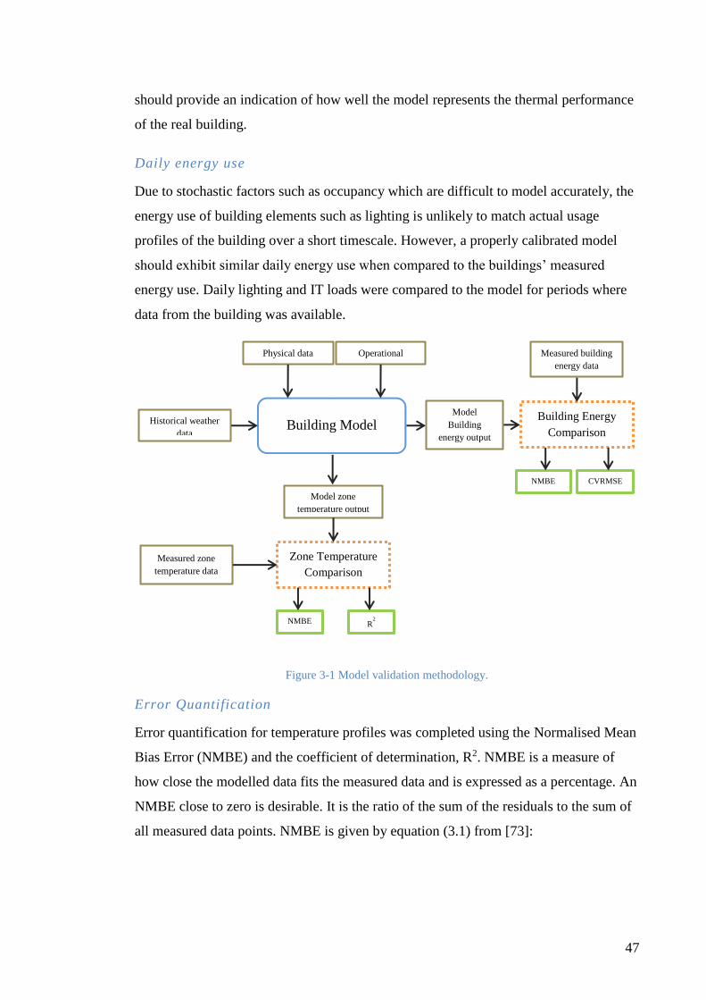
47
should provide an indication of how well the model represents the thermal performance
of the real building.
Daily energy use
Due to stochastic factors such as occupancy which are difficult to model accurately, the
energy use of building elements such as lighting is unlikely to match actual usage
profiles of the building over a short timescale. However, a properly calibrated model
should exhibit similar daily energy use when compared to the buildings’ measured
energy use. Daily lighting and IT loads were compared to the model for periods where
data from the building was available.
Figure 3-1 Model validation methodology.
Error Quantification
Error quantification for temperature profiles was completed using the Normalised Mean
Bias Error (NMBE) and the coefficient of determination, R2. NMBE is a measure of
how close the modelled data fits the measured data and is expressed as a percentage. An
NMBE close to zero is desirable. It is the ratio of the sum of the residuals to the sum of
all measured data points. NMBE is given by equation (3.1) from [73]:
R2
Building Model
Physical data Operational
profile
Historical weather
data
Zone Temperature
Comparison
Measured zone
temperature data
Model zone
temperature output
NMBE
Model
Building
energy output
Building Energy
Comparison
NMBE CVRMSE
Measured building
energy data

48
𝑁𝑀𝐵𝐸 = ∑(𝑦𝑚𝑒𝑎𝑠𝑢𝑟𝑒𝑑 − 𝑦𝑚𝑜𝑑𝑒𝑙𝑙𝑒𝑑)
∑ 𝑦𝑚𝑒𝑎𝑠𝑢𝑟𝑒𝑑
×100 (3.1)
Where:
▪ ymeasured = measured data point
▪ ymodelled = modelled data point
A maximum NMBE of 15% was considered as satisfactorily accurate for the thermal
validation of the model. As thermal accuracy of the model is secondary to that of energy
and serves only to confirm the correct behaviour of the building model, there are no
specific acceptability criteria being followed for the thermal model. An NMBE of 15%
was chosen as this corresponds to an average residual of around 1-2°C, which is within
the margin associated with measurement error such as calibration or position of
measurement. Regardless of the allowable error selected the model will always be more
accurate in some sections of data than others owing to unpredictable events such as
occupant override of building HVAC systems or equipment malfunction. Additionally,
the coefficient of determination, R2, was calculated from a scatter graph between
measured and modelled temperature variables. This helped to quantify the degree of
correlation between the model and the real building and aided in setting levels of
confidence in the model.
The error associated with the energy models was quantified according to the method
outlined in ASHRAE Guideline 14-2002 [73]. This method relies on measured energy
data being compared to the model output using both the NMBE and the Coefficient of
Variation of the Root Mean Squared Error (CVRMSE). The CVRMSE is a measure of
how well the model fits the data. A lower CVRMSE value suggests that the model is a
better fit. It is the ratio of the square-root of the Mean Bias Error to the average of all
measured data points.
CVRMSE is given by equation (3.2):
𝐶𝑉𝑅𝑀𝑆𝐸 = √(𝑦𝑚𝑒𝑎𝑠𝑢𝑟𝑒𝑑 − 𝑦𝑚𝑜𝑑𝑒𝑙𝑙𝑒𝑑)
2
��𝑚𝑒𝑎𝑠𝑢𝑟𝑒𝑑
×100 (3.2)
Where:
▪ ymeasured = measured data point
▪ ymodelled = modelled data point
▪ ӯmeasured = average of all measured data points

49
The CVRMSE is used in conjunction with NMBE to eliminate the fact that NMBE may
be influenced by offsetting errors. ASHRAE Guideline 14 states that an energy model
may be declared valid if the NMBE is ±10% and the CVRMSE within ±30% when
using hourly data or 5% to 15% when using monthly data. Although daily data is being
used here, the 15% limit was chosen for the selected case study simulations. The
building models developed in this study are intended to be generally representative of
the real buildings so that general behaviour can be simulated.
3.3 Simulation methodology
Development of a simulation methodology must reflect the overall objectives of the
project. As whole-building energy use was of particular focus here, overall energy
consumption is the main metric to be used to indicate results of different simulations.
However a deeper understanding may be gained by looking at a system or sub-system
level. In a system as complex as a building, there are many combinations of variables
that may have an effect on energy use. It would be impractical to investigate all of them
for the purposes of this thesis. Five building elements were selected to be investigated in
terms of their technology and their implementation. The proposed simulation
methodology is outlined in Figure 3-2.

50
Figure 3-2 Proposed building simulation methodology.
In some cases, it is necessary to maintain a constant level of certain parameters in the
interests of occupant comfort. It would not be acceptable for a building to achieve large
energy savings if this comes at the expense of occupant comfort and building
functionality. For the case of lighting, it is necessary to keep an adequate and reliable
standard of illuminance. Where shading is concerned, both lighting and IEQ are
influenced and thus must be maintained where different shading technologies and
control strategies are investigated. In some cases, occupant comfort and functionality
are the variables being tested, rather than maintained. For the investigation of HVAC,
the temperature bands are to be varied to determine the amount of energy that could be
saved if occupants were willing to tolerate slightly warmer conditions in summer and
cooler conditions in winter.
The following figures outline the procedures followed for the simulations of each
building model.
Validated Building Model TMY weather data
C. Window Shading -Time of day/Seasonal -Maximum outside
Temperature
D. HVAC Set Point Control -Heating ±1°C increments - Cooling ±1°C increments
A. Glazing type -Single/Single LowE -Double/Double LowE -Triple/Triple LowE
B. Lighting Output Control -Control on -Control off
Simulation Scenarios
C. Window Shading -Total yearly HVAC energy (kWh) - Total yearly lighting energy (kWh) -Total yearly building energy (kWh)
A. Glazing type -Total yearly HVAC energy (kWh) -Total yearly lighting energy (kWh) -Total yearly building energy (kWh)
D. HVAC Set Point Control -Total yearly HVAC energy (kWh) -Total yearly building energy (kWh)
B. Lighting Output Control -Lighting energy intensity (kWh/m
2)
-Total building energy intensity (kWh/m2)
Scenario Performance Indicators

51
3.3.1 Glazing
Changing the type of glazing is likely to have an impact on the solar heat gains in the
building throughout the year. Single glazed or poor performance double glazed
windows are likely to introduce more heat to the building throughout summer, driving
up cooling loads. Figure 3-3 outlines the simulation process to be carried out.
Figure 3-3 Glazing simulation procedure.
The overall annual impact on HVAC energy use will be tested here as well as the
impacts on other related electrical systems such as lighting. It is hoped that the outcome
will be a quantification of any benefits of high quality double glazing and whether triple
glazing could extend those benefits in any significant way.
3.3.1.1 A description of glazing types
It is important to outline the different types of glazing examined in this study to give
some background and insight into why these building elements are being simulated.
Single Glazing
A conventional single pane of glass mounted in a frame typically constructed of timber
of aluminium.
Single LowE Glazing
Similar to a single glazed window, but using low emissivity glass (LowE). LowE glass
has a thin coating deposited on its surface. Different coatings can have different effects
Set model parameters
•Set model lux levels and temperature set points to be maintained throughout all simulations
•Set window shading to zero
Run simulations
•Single/Single LowE
•Double/Double LowE
•Triple/Triple LowE
Analyse results
•Compare results to single glazed benchmark using the following metrics:
•HVAC energy use
•Lighting energy use
•Overall energy use

52
but typically, all coatings cut down on the amount of infrared light being transmitted
through the pane. This has the effect of reducing radiant heat transfer.
Double Glazing
A window system consisting of two panes of glass mounted in a frame typically
constructed of timber of aluminium. The gap between each pane of glass is commonly
filled with air. Argon can also be used to provide improved insulative properties
Double LowE Glazing
Similar to conventional double glazing, but using LowE glass as previously described
for one or both panes.
Triple Glazing
Similar to a double glazed window unit, however three panes are used instead of two.
Triple LowE Glazing
Similar to conventional triple glazing, but using LowE glass as previously described for
one or all three panes.
3.3.2 Lighting
Whilst there are many different types of lighting technology available, their impacts on
electrical loads are relatively easy to calculate without the need for modelling given that
their electrical inputs are generally proportional to their light outputs. Instead, the
operation and control of lighting will be simulated as this relies on many different
variables. Daylight control involves the use of a photosensor to detect the amount of
natural light in the room. The lighting control system interprets the reading given by the
photosensor and decides how much artificial light is necessary based on preset lighting
level requirements.
Occupancy also plays an important role in lighting operation. A modern controlled
lighting system will be occupancy-driven. Passive Infrared (PIR) sensors will detect
occupancy and automatically turn on artificial lights if they are necessary. An additional
simulation scenario of determining the energy savings due to automatic lighting control
would be of great interest. However occupancy can be difficult to predict in many
situations (especially for sparsely populated buildings) and the models presented here
do not have the capability to model stochastic factors such as occupancy. For the

53
purposes of this study, lighting operation is driven by a predetermined occupancy
schedule. Figure 3-4 outlines the simulation and analysis procedure to be followed.
Figure 3-4 Lighting simulation procedure.
The lighting schedules for each building model are shown below in Figure 3-5.
Figure 3-5 Building model lighting schedules
The occupancy schedules for each building model are shown below in Figure 3-6.
Occupancy and building systems schedules have significant influence over the results of
a simulation and are key factors in developing an accurate and validated model.
Set model parameters
•Set model lux levels to be maintained throughout all simulations
Run simulations
•Perform simulations comparing non-controlled lighting to proportionally controlled lighting through the use of daylight sensors
Analyse results
•Compare results using the following metrics:
•Lighting energy use intensity
•Overall energy use intensity

54
Figure 3-6 Building model occupancy schedules
3.3.3 Window Shading
Local shading of windows using architectural elements, such as side fins, overhangs,
and louvres is driven by well researched architectural design and depends heavily on the
building site location and orientation. This would be a challenging building element to
model and drawing general conclusions from the results would be problematic.
However, window shading in the form of blinds or curtains can be modelled with
expected conclusive outcomes.
Figure 3-7 Window shading simulation procedure.
Set model parameters
•Set model lux levels and HVAC setpoints to be maintained throughout all simulations
Run simulations
•Slatted blind - high reflectivity
•Summer day/night
•Winter day/night
•Temperatures above 25/28/30/32°C
Analyse results
•Compare results to benchmark of no shading using the following metrics:
•HVAC energy use
•Lighting energy use
•Overall energy use

55
Rather than simulation of the best type of shading, which could have many
combinations, the operation of the window shading has been chosen for modelling
instead, as outlined in Figure 3-7. A consistent shading type has been chosen as a slatted
blind with high reflectivity slats. The reason for this is that this type of shading is
common in many commercial buildings. The scenarios to be tested are based both on
the season and time of day, as well as the outdoor temperature. The results will be
compared on a whole building energy use level, as well as the impacts on lighting
energy use (with less natural light in summer, this will increase lighting loads) and
HVAC use.
3.3.4 HVAC
Since detailed HVAC systems in DesignBuilder are quite complex to model, a
simplified model will be developed for the case study buildings. A result of this is that
the HVAC energy consumption of the model is likely to be only nominally comparable
to that of the real system. However, the relative performance effects of the model
system amongst the simulated scenarios will still be valid and conclusions about energy
consumption changes may still be drawn back to the real system.
Figure 3-8 HVAC simulation procedure.
Keeping HVAC simulations independent of equipment specifics enables general
conclusions to be made about potential energy consumption in buildings. Varying the
HVAC setpoints is often quoted as an effective way of reducing energy consumption
[74]. Simulations performed in this study will aim to quantify this effect for the net zero
energy test cases as well as more generally. Figure 3-8 outlines the simulation process
Set model parameters
•Set model lux levels to be maintained throughout all simulations
Run simulations
•Cooling setpoint variation: ± 1.0°C increment
•Heating setpoint variation: ± 1.0°C increment
Analyse results
•Compare results to each buildings real HVAC settings using the following metrics:
•HVAC energy use
•Lighting energy use
•Overall energy use

56
to be carried out. The HVAC operation schedules used in each building model are
shown in Figure 3-9.
Figure 3-9 Building model HVAC schedules
3.4 Sustainable Buildings Research Centre – University of
Wollongong
The University of Wollongong’s Sustainable Buildings Research Centre (SBRC),
shown in Figure 3-10 was designed to bring together a range of disciplines with the goal
of addressing the challenge of making Australian buildings more sustainable. The
location of the 8,000 m2 site of the building is at the Innovation Campus of the
University of Wollongong. It is a 2,600 m2 double story research building with
exhibition spaces, education and training centres, as well as academic offices and high-
bay laboratories. With the building axis running east-west and separation between the
two main wings, maximum passive ventilation and natural light are utilised. The first of
the two wings is a 1,700 m2 building housing academic offices, education and training
spaces, as well as a flexible working space and public exhibition centre. The second
wing is a 900 m2 structure housing high-bay laboratories and much of the HVAC plant
used in the building.

57
Figure 3-10 Sustainable Buildings Research Centre (SBRC).
3.4.1 Building façade
Key features of the building façade of the SBRC building are the reverse brick veneer
construction, which differs from conventional brick veneer construction by placing the
thermal mass on the inside of the building, within the insulated envelope. This provides
a more stable indoor temperature [75]. A mixture of timber and steel cladding is used on
the exterior of the building. An example of the insulated timber and steel façade section
is shown in Figure 3-11.

58
Figure 3-11 SBRC building façade section example [76].
The building is insulated to a high degree. Concrete slabs are insulated to a minimum R-
value of 3.2 m2K/W. External walls are insulated typically with 90 mm thick polyester
batts with a minimum R-value of 2.8 m2K/W. Roof insulation is specified as a
minimum R-value of 3.2 m2K/W.
Primarily, high performance double glazing is used for all external windows, glazed
doors, and curtain walls. Windows are fitted with actuators controlled by the BMS when
natural ventilation is deemed necessary.
3.4.2 Energy efficiency
The SBRC achieves its high level of energy efficiency thanks to a range of design
choices and cutting edge technologies.
The building is laid out in an H-configuration. This helps to optimise natural ventilation
and maximises natural light throughout the building. A mixed-mode ventilation system
utilizing a ground heat exchanger and in-slab hydronics system reduces the HVAC
energy intensity significantly over a more conventional system. Low energy lighting
systems with intelligent controls are used where daylight levels are insufficient. PIR
sensors detect if a room is occupied and photoelectric light sensors detect whether
daylight levels are low enough to warrant the use of artificial lighting.
59
3.4.3 Local generation
Solar PV arrays are installed on both north and south wings of the SBRC providing a
total capacity of 163 kWp. The south wing rooftop holds most of the installed capacity
with 120 kWp whilst 43 kWp is installed on the north wing of the building in two
different inclinations – 30° and 70°.
In addition to the conventional PV installed at the SBRC, an experimental array of
Building Integrated Photovoltaic Thermal (BIPVT) panels has been installed. Ducts
installed beneath the panels harvest the heat absorbed by the PV panels. This not only
increases the efficiency of the panels, but the collected heat can also be put to use
elsewhere in the building for space heating if required.
The Illawarra Flame, the University of Wollongong’s winning entry in the 2013 Solar
Decathlon, is also situated nearby on campus. It is fitted with both conventional PV and
BIPVT and is also connected via the SBRCs electricity distributions system, providing
additional generating capacity to the precinct on top of that provided by the SBRC.
3.4.4 Description of Building Systems
3.4.4.1 HVAC
The HVAC system at the SBRC is able to operate in three modes – natural ventilation,
heating, or cooling. Natural ventilation is implemented through the use of automated
windows and louvres on the building envelope. It is designed to be the primary space
conditioning mode for maintaining the building within 20°C and 24°C. Outside of this
comfort band, mechanical heating and cooling modes are used. The main mechanical
plant equipment are as follows;
• One air cooled heat pump;
• Two water-cooled heat pumps;
• Six variable speed water pumps;
• One ground loop header pump;
• Supply and return water temperature sensors;
• Eighteen motorized flow diverting or control valves;
Ground-source heat exchange loops are used to exchange heat with the stable
temperature of the ground. A variable speed water pump is fitted to the ground loop to
maintain constant pressure to the system.

60
Operation preference is given to the Ground Source Heat Pumps (GSHP) as they are
generally more efficient over the air source heat pump (which is used only to meet peak
loads or in the event of GSHP equipment malfunction or servicing) due to its use of
ground heat exchangers where the temperature is more suitable than the atmosphere for
use as a heat source or sink.
3.4.4.2 IT system
Low energy Virtual Desktop Infrastructure (VDI) is used at the SBRC instead of
traditional separate PC terminals. Each desk has only a display monitor, keyboard, and
mouse, all powered over Ethernet connection with processing hardware located off site
in a concentrated server configuration. A thin-client VDI terminal consumes around 8-
20 W of energy compared to an average of 150 W for a traditional PC [77]. A VoIP
phone system is used in place of traditional phone systems, further cutting down on
energy use.
3.4.4.3 Lighting
Low energy lighting systems are used at the SBRC with occupancy sensors and daylight
harvesting strategies implemented. Lights only operate once occupants are sensed or if a
manual input is received from a lighting control panel. Lights remain on for a
programmed amount of time after sensed occupancy ceases. Photoelectric sensors
control lighting fixture output according to natural lighting levels in the zone.
The lighting system is designed to reduce general ambient lighting intensity in favour of
more concentrated task-based lighting. Main office spaces may be lit to a lower level
than that of a more conventionally lit office, however more focussed task lighting
makes up for this at work surfaces. This reduces the amount of wasted light by
supplying it only where needed.
3.4.5 Energy monitoring
A number of energy monitoring systems are employed at the SBRC:
Building Management System
The Tridium Niagara Building Management System monitors and records a number of
electrical meters in the building at 15-minute time intervals. This data is logged and can
be accessed at any time from the BMS server. Some meters of note are:
• Main Supply

61
• PV North array
• PV South array
• Mechanical services
• BIPVT
Remaining meters measure the plug, lighting, and IT loads which are separated into
ground floor, first floor, laboratory, and high bay zones.
Meters are also placed on individual items of HVAC equipment such as heat pumps,
fans, and water pumps. Provision is also made for future installations such as wind
turbines, electric vehicle charging stations, and other experimental distributed
generation. These meters are capable of measuring active, reactive, and apparent power,
as well as the current, voltage and frequency of all phases and some power quality
parameters such as total harmonic distortion and power factor.
Solar-Log
Additional metering of the solar arrays is possible through the online monitoring
services provided by the solar installer. Energy production is logged at 5-minute
intervals and can be broken up into contributions from the north and south arrays.
Monthly and yearly summaries are also prepared automatically. In addition to energy
production, the condition of the inverters can also be assessed through this service with
the temperature and efficiencies of each inverter being logged. Inverter input voltage is
also measured.
Portable IEQ and PQ meters
Where more in-depth metering capabilities may be needed, or if metering is not
available on a specific component, portable power quality meters are also available to
connect to the SBRC circuits on a rotational basis. These are capable of providing high
resolution, detailed data and can be interfaced in a variety of ways including LAN for
remote meter reading.
3.5 Transformational Technical Training Building – TAFE NSW
The TTT building, shown in Figure 3-12, is located at the Yallah campus of TAFE
NSW was built as part of the joint funding initiative which also funded construction of

62
the SBRC. The TTT building is designed as a net zero energy and water building and
aims to achieve Living Building Challenge certification much like the SBRC. The
building is used for educational, training, and demonstration purposes by the TAFE
Illawarra Institute, as well as the surrounding civic and business communities.
Figure 3-12 Transformational Technical Training (TTT) building.
The TTT building is a 1,020 m2 facility featuring 500 m2 of teaching space including
185 m2 of practical laboratory training space on the 800 m2 first floor. 100 m2 of
administration office space and reception is located on the ground floor.
3.5.1 Building façade
Much like the SBRC building, a high level of insulation is present at the TTT building.
Block-type wall construction is used on the ground floor where the building is cut into
the slope of the ground. Steel framed external walls, clad in fibre cement panels are
used on the first floor. Minimum R2.5 insulation is used in external walls.
External windows and glazed doors consist of a combination of double glazing and high
performance single glazing.
3.5.2 Energy efficiency
As a net zero energy building, a number of energy efficient design features are present.
Large north-facing windows with high performance glazing are used to maximise the

63
amount of natural lighting. Artificial lighting is all LED and is controlled by occupancy
sensors.
The building is north facing and has large roof overhangs to reduce summer solar heat
gains but allow winter solar gains into the building. A solar hot water system is
installed, significantly reducing loads associated with DHW heating.
3.5.3 Local generation
A solar PV system is installed with capacity of 28 kWp. Approximately 40 MWh of
energy is generated annually.
3.5.4 Description of Building Systems
HVAC services include a 60 kW GSHP system supplying heating and cooling to
teaching spaces on the first floor. The common area and horticulture labs on that floor
are both naturally ventilated. On the ground floor, a separate conventional ASHP
system services the office and reception areas. Refer to water and air schematics of TTT
in Figure 3-13 and Figure 3-14, respectively.
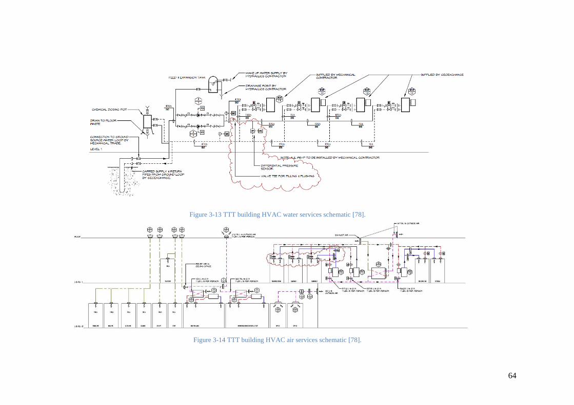
64
Figure 3-13 TTT building HVAC water services schematic [78].
Figure 3-14 TTT building HVAC air services schematic [78].

65
3.5.5 Energy monitoring
Energy monitoring is capable through the Delta Controls BMS. Sub metering is
available for electrical circuits as outlined below in Figure 3-15 using EP&T G3
intelligent meters connected to the BMS.
Figure 3-15 TTT electrical meters and sub-meters.
The ‘Hydraulics’ meter includes all energy involved with pumping and treating of the
rainwater supply, as well as pumping of ground heat exchanger fluid for the GSHP
system.
3.6 Enterprise 1 – University of Wollongong
Enterprise 1, another building situated at the University of Wollongong’s Innovation
Campus, is a commercial office building whose tenants include multinational
corporations and UOW research institutes. It is a three-story building with a total floor
size of around 10,000 m2 and was opened in 2011.
3.6.1 Building façade
The building consists of a concrete framed shell with lightweight curtain wall cladding.
Operable slatted timber louvres (shown in Figure 3-16) provide shade at the east and
west ends when needed. External windows are double glazed with aluminium frames.
The insulation installed in the external cladded walls achieves an R-value of 2.5.
TTT Main Incomer
HVAC 1
HVAC 2
HVAC 3
Lift
L00 Power L01 Power
L00 Lighting L01 Lighting
Hydraulics

66
Figure 3-16 Enterprise 1 building east/west timber louvres [79].
3.6.2 Energy efficiency
The building has been designed to achieve a minimum 5 star NABERS base-building
rating. A base-building rating concerns the greenhouse gas emissions associated with
energy consumed by core building services such as common area lighting, lifts, HVAC
central plant (not including supplementary HVAC used by tenants), and exterior
lighting. The base building assessment does not consider energy consumed by tenancy
activities.
The 5-star base-building rating means the building can be considered as state-of-the-art
for a building of its type and one which is a good candidate to be compared against net
zero energy buildings. Occupancy controls on office lighting systems aim to reduce
unnecessary lighting use, as well as in bathroom areas where lights are switched off
after a 1 hour period with no detection. Low energy compact fluorescent downlights are
used, along with T5 linear fluorescent fittings in offices. This gives a resulting overall
lighting power density of 9.4 W/m2, which can be calculated from electrical plans and
equipment schedules in the operation and maintenance manuals for the building

67
3.6.3 Description of building systems
Mechanical HVAC equipment installed in the Enterprise 1 building includes 2 x
600 kW chillers. These are designed so that either of the two chillers is able to provide
50% of maximum demand. 2 x 202 kW gas fired boilers are installed to meet heating
demand. All of the 13 Air Handling Units (AHU’s) are equipped with variable speed
drives. The measured total yearly HVAC energy consumption of the building for 2014
was approximately 373,000 kWh.
The lighting system as previously described is metered in combination with general
plug loads. The combined yearly energy consumption of light and power was
approximately 1,082 MWh. It was estimated that the contribution of lighting to this
combined load is 492 MWh, based on the model developed for this research which uses
lighting specification inputs described above. Two lifts operate between the three
above-ground floors and the basement carpark. These contribute around 8,000 kWh per
year to overall energy consumption.
3.6.4 Energy monitoring
Less data is available for the building loads in Enterprise 1 as this is a much more
conventional building and metering is less extensive. However, due to the NABERs
rating requirement, electrical, gas, and water metering is required for key building
systems so that consumption of these sources can be factored in the annual NABERS
assessment. The electrical meters of interest in this study are:
• Incoming mains
• 3 HVAC meters measuring water pumps, cooling towers, pumps, chillers,
AHU’s, and other ventilation fans
• Base-building light and power
• Tenant light and power
3.7 Summary of building features
A brief summary of the key building features for all case study buildings is given in
Table 3-1. These features may have a significant bearing on the overall energy
performance of the building and the benchmark model for each case study will be
constructed around these features.

68
Table 3-1 Summary of building features
TTT SBRC Enterprise 1
Occupancy Type Education and Training Education, Research and Training Commercial
Approx Number of Occupants 150 50 900
Number of Floors 1 2 4
Total Floor Area 1 021 2 600 11 874
Wall Type Combination of concrete
blockwork and metal
clad/steel frame
Combination of concrete and steel
framing, with recycled brick and
timber cladding facade
Concrete with curtain
wall cladding
Wall Area 813 2 261 3 730
Glazing Type Combination of double
glazing and high-
performance single
glazing
Double glazing Double glazing
Glazing Area 218 652 2 261
Lighting Type LED LED T5 Fluorescent T-Bar
Troffer in office spaces
Lighting Control Motion sensor & PE cell Motion sensor & PE cell Control schedule and
motion detection after
hours
Average Lighting Level 193 213 320
Lighting Power Density 4.75 1.60 9.40
HVAC Type 3x Reverse cycle
geothermal heat pumps
(total cooling capacity
45 kW)
1x water-cooled VRF-
type heat pump (total
cooling capacity 27 kW)
1x Air-cooled reverse cycle
chiller (total cooling capacity
110 kW)
2x Reverse cycle geothermal heat
pumps (total cooling capacity
34 kW)
Central chilled water
system (total cooling
capacity 1200 kW)
Central gas-fired hot
water system (total
heating capacity
400 kW)
Cooling Setpoint 24.5 24.5 24.0
Heating Setpoint 19.5 19.5 21.0
3.8 Summary
In this chapter, the purpose and methodology for simulation of the case study buildings
has been presented, as well as details on the buildings themselves. The uncertainties that
may cloud simulation results such as unpredictable weather conditions and occupant

69
behaviour were considered and a validation methodology was presented to account for
these uncertainties.
The schedule and methodology of simulations was outlined for glazing, lighting control,
window shading, and HVAC setpoint. Case study buildings to be simulated were
introduced with a description of their construction and features, including energy
efficient building technology and energy monitoring equipment that may be installed.

70
Chapter 4 Model Validation & Performance Simulation
4.1 Purpose of building simulation
The work in this chapter focusses on modelling and simulation of energy consumption
related to different building scenarios for the three test cases introduced in Chapter 3.
Through simulation, it is possible to investigate the impact on energy consumption
caused by utilising different construction materials, appliances, lighting systems, etc. in
the building design as well as how occupants interact with a building which might
otherwise be impractical or impossible to investigate in reality. Verification of the three
case study building models is an essential step towards having confidence in the results
of the simulations performed in the next chapter. The outcomes of these simulations
will demonstrate the effects on whole-building energy consumption that different
building elements or parameters may have had and how this may impact the future
design of net zero energy buildings.
4.1.1 Relevance to net zero energy
When considering net zero energy building principles, reduction of energy requirements
is at the forefront of objectives. Simulating different building technologies, operating
parameters and usage schedules enable a designer to optimise the design of a building to
use the least amount of energy possible, reducing the capacity or operation time of
renewable energy required to achieve net zero.
In such a complex system as a building, altering one parameter to achieve a positive
outcome in one aspect may have a detrimental effect on other aspects. One example of
this is to introduce a window shading solution such as blinds or curtains. In summer,
shading the windows during the day likely diminishes the effect of solar gains on the
building, potentially lowering the cooling load and hence the electricity required by the
HVAC system. However, a consequence of covering windows during the day is that the
amount of daylighting is reduced, therefore requiring an increase in interior artificial
lighting and hence an increase in the electricity required to light the building to a
comfortable level. To complicate matters further, whilst the HVAC loads are reduced by
implementing window shading, the increase in artificial lighting required as a result
generates heat and potentially increases HVAC loads in some situations.

71
Building modelling and simulation provides a way of quantifying the effects of such
interdependent systems. In the above case, simulation would enable the designer to
decide whether or not window shading would be the most effective approach to
improving energy efficiency, or whether the added lighting energy required and the
potential cooling load increase from waste heat has a negative impact on the overall
energy consumption of the building.
In this project, several interdependent scenarios similar to the example above will be
investigated using building simulation. DesignBuilder [80] is chosen for this given that
it is readily available, user friendly, and crucially, provides a demonstrable level of
accuracy. It is necessary to determine the sensitivity of the building to changes such as
type of window shading, lighting, HVAC system, and construction materials used, as
well as the way in which the various technologies are implemented. The aim of
simulating these scenarios is to minimise the overall building energy consumption with
a view to achieving net zero energy status when all factors of the different building
systems are considered, as well as to determine the contribution that energy efficient
technology may make to overall energy savings to a building in a broader sense.
4.2 Planned outcomes of simulations
The application of the simulation methodology described in Section 3.3 was planned for
implementation to each of the three test cases. The planned outcomes of the simulations
were as follows (noting that it was anticipated that the outcomes would have relevance
beyond the case study buildings, i.e. would be applicable to efficiency improvements in
the built environment in general):
• Gain an understanding through simulation of how different building elements
interact through a variety of scenarios and what consequences this interaction
may mean for whole-building energy intensity in a broader context;
• Make comparisons between benchmark and simulated scenario data to
determine the overall contribution to energy savings that each energy efficient
technology makes;

72
• Enable discussion on the potential for improvement of current building codes
and operating procedures concerning the energy efficiency of building
components.
4.3 Background of models
The case study buildings include two net zero energy buildings and one modern
commercial building. The two net zero buildings are small educational facilities – one
approximately 1,000 m2 and the other approximately 3,000 m2. The commercial
building is approximately 10,000 m2.
Despite the differences in purpose and size between the net zero educational buildings
and the commercial building, meaningful conclusions were expected to be drawn from
the comparisons made between simulation results for the three buildings.
4.3.1 TTT
The DesignBuilder model of the Transformation Technical Training (TTT) building at
TAFE Illawarra’s Yallah Campus in NSW, Australia, was developed using
architectural, mechanical, and electrical drawings sourced from the project manager of
the building construction. The building floor plan was modelled as specified in the
drawings, as were all glazing elements and lighting specifications. Some simplifications
were made to the model where deemed either too complicated to model, or would have
had little bearing on the simulation results, such as the finer details of the roof design in
some areas.
As the DesignBuilder library has an extensive, but not exhaustive library of building
materials, good approximations were found for wall, roof, and floor construction
materials, as well as insulation and window glass. A visualisation of the TTT building
model developed in DesignBuilder is provided in Figure 4-1, illustrating the external
layout of the building.

73
Figure 4-1 TTT building model physical geometry as modelled in DesignBuilder.
The lighting specifications and the required lighting intensity levels for each building
zone were included in the provided design details, so it was relatively straightforward to
enter this data into the model to provide the specific lighting output. The design level of
lighting output was adjusted to suit the DesignBuilder requirement of specifying
lighting units in W/m2/100 lx. Using these units allows for variation between the
different case study buildings. Each building has varying lighting requirements and
comparing them on a lighting power density basis alone would not provide a fair
comparison. Introducing the lux levels in the lighting specification allows for fair
comparison between buildings.
For example, Building 1 has an installed lighting power density of 5 W/m2 and is
required to achieve an overall lighting level of 100 lx. This results in a lighting
specification of 5 W/m2/100 lux. Building 2 has a lux level of 240 and a lighting power
density of 6.5 W/m2. The lighting specification for Building 2 is 2.71 W/m2/100lx. It is
illustrated that although the lighting power density in Building 2 is higher than that of
Building 1, the lux level required is also higher. Building 2 is more efficient at
achieving its required lux level than Building 1.
As lighting in the building is controlled primarily by zone occupancy, lighting operation
schedules were assumed to closely align with building occupancy schedules. These
were both approximated based on the energy use data, which tends to be indicative of
building occupancy and occupant behaviour to some degree, and were also correlated
with anecdotal evidence from staff occupying the building of general occupancy
periods. Additionally, daylight lighting control was used to adjust the output depending
on the amount of natural light entering the room.
74
The HVAC system was modelled using the Simple mode in DesignBuilder. This
reduces the complexity of the model by eliminating the requirement to specify every
element of the HVAC system – a complex and intensive process. Instead, Simple mode
uses an idealised load calculation method which utilises constant coefficients of
performance as specified by the modeller [80]. It is possible to specify the energy
associated with pumps and fans separately which can be determined using BMS energy
data. Because Simple mode is used, the energy model for HVAC is not expected to be
as accurate as other aspects of the model when compared to the real building, however
relative changes in energy use should still be valid across model results since the HVAC
model specification will be consistent.
The natural ventilation mode during simulation was Scheduled as opposed to the more
complex alternative of allowing DesignBuilder to determine through calculation (i.e.
Calculated mode). Scheduled sets a nominal air flow rate for the zone and is controlled
by an operation schedule. Natural ventilation can occur if zone temperatures and outside
temperatures are within the prescribed temperature bands and as long as the schedule
allows. This is different to the Calculated mode which, instead of using a nominally
specified air flow rate, calculates the flow rate based on outside conditions such as wind
direction and velocity, and window design. As sufficient results were achieved using
scheduled natural ventilation, Calculated mode was not necessary and further model
simplification was achieved.
Air infiltration was left at the default constant value of 0.7 air changes per hour (ac/h) as
specified by the standard DesignBuilder modelling template. This value was left at the
default as no measured data from air permeability tests was available to better inform
the model. It was assumed that air infiltration was constant at all times due to it being
infeasible to test for this. A constant infiltration rate was assumed across all three
buildings being studied.
As little data was available about electrical equipment in the building, assumptions had
to be made based on the small amount of energy data which was available. This energy
data included HVAC loads, lighting loads, and general purpose outlet (GPO) loads for
the first three months of 2015; two summer months and the first month of autumn.
Generic loads were then specified in the model with the intention to represent all
general electrical equipment such as computers, desk lamps, kitchen appliances, etc.
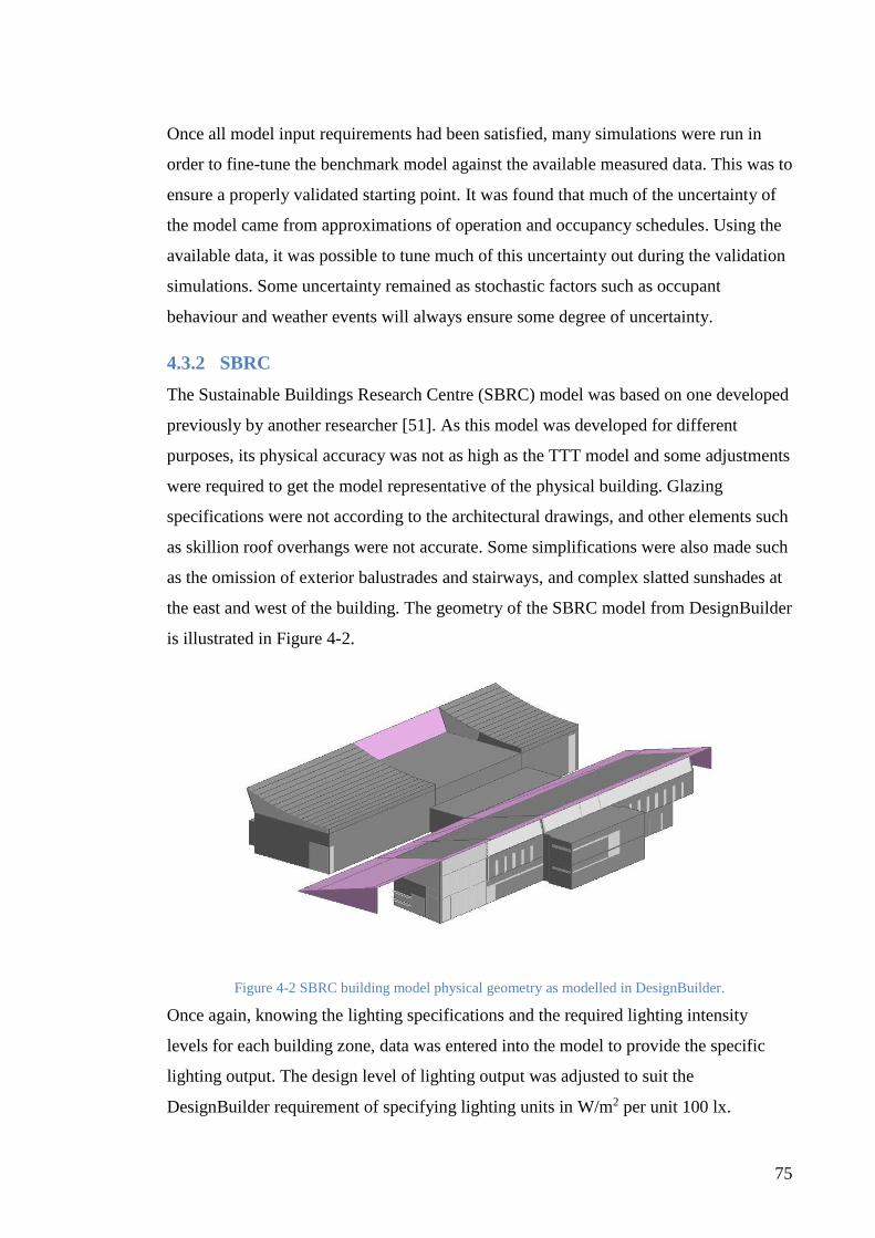
75
Once all model input requirements had been satisfied, many simulations were run in
order to fine-tune the benchmark model against the available measured data. This was to
ensure a properly validated starting point. It was found that much of the uncertainty of
the model came from approximations of operation and occupancy schedules. Using the
available data, it was possible to tune much of this uncertainty out during the validation
simulations. Some uncertainty remained as stochastic factors such as occupant
behaviour and weather events will always ensure some degree of uncertainty.
4.3.2 SBRC
The Sustainable Buildings Research Centre (SBRC) model was based on one developed
previously by another researcher [51]. As this model was developed for different
purposes, its physical accuracy was not as high as the TTT model and some adjustments
were required to get the model representative of the physical building. Glazing
specifications were not according to the architectural drawings, and other elements such
as skillion roof overhangs were not accurate. Some simplifications were also made such
as the omission of exterior balustrades and stairways, and complex slatted sunshades at
the east and west of the building. The geometry of the SBRC model from DesignBuilder
is illustrated in Figure 4-2.
Figure 4-2 SBRC building model physical geometry as modelled in DesignBuilder.
Once again, knowing the lighting specifications and the required lighting intensity
levels for each building zone, data was entered into the model to provide the specific
lighting output. The design level of lighting output was adjusted to suit the
DesignBuilder requirement of specifying lighting units in W/m2 per unit 100 lx.

76
Lighting schedules were determined from BMS lighting energy use data. It was possible
to develop a schedule to follow the underlying trends present in the energy data for the
interior and exterior lighting of the building. Lighting daylight control during the day is
also used to adjust the output depending on the amount of natural light entering the
room.
Like the TTT, the HVAC system for the SBRC was modelled using the Simple mode in
DesignBuilder. Energy associated with pumps and fans is specified separately and is
informed from viewing BMS energy data.
The natural ventilation mode used was ‘Scheduled’. Air infiltration was applied
building-wide at 0.3 ac/h in accordance with the targeted infiltration rate being less than
0.5 as specified in the SBRC building users guide. It was assumed that air infiltration
was constant at all times.
Generic loads in the model were specified based on BMS electrical data. These are
intended to represent all general electrical equipment such as computers, desk lamps,
kitchen appliances etc.
As with the TTT building model, benchmarking simulations were performed in order to
establish model validation against measured data. Uncertainties associated with
operation schedules were eliminated as much as possible, and window shading detail
was added to cut down on solar gains into the building which appeared to give
unrepresentative temperature results due to the large glazed curtain walls on the western
end.
4.3.3 Enterprise 1
The Enterprise 1 model was built from scratch using the architectural drawings. The
building façade has been simplified due to the high number of windows resulting in an
unacceptable simulation time. The total window area however has been accurately
represented. Glazing type for the model was specified as double glazed clear. Figure 4-3
shows the model geometry of the Enterprise 1 building model.

77
Figure 4-3 Enterprise 1 model physical geometry as modelled in DesignBuilder.
The air infiltration rate assumed for the Enterprise 1 model is 0.7 ac/h, and this is
assumed to be constant at all times. Simple HVAC mode is used here to reduce
modelling complexity, with the auxiliary loads being specified separately, just as they
are done with the other two models.
Lighting densities for the model were specified according to those outlined in the
Enterprise 1 building construction documentation. An average base lighting power
density of 9.4 W/m2 was calculated based on the primarily 28 W T5 fluorescent lighting
fixtures installed throughout the majority of spaces in the building.
4.3.4 Summary
With the models being created to the highest level of accuracy according to the details
available, there are still unknowns and assumptions made which may affect the
behaviour and results of the models. To reduce errors associated with these
assumptions, it is necessary to perform a validation process for each of the models to
ensure they will give reliable and representative results.
4.4 Validation of models
To ensure that building models are an accurate representation of reality and that their
data outputs are reliable, it is critical that they are properly validated and verified so that
they can be relied on to give useful conclusions about net zero energy buildings. By
comparing the data generated by the models with analogous data measured from the real
buildings, and coupling this with a weather file in the model created from actual
measured data from a site nearby to the building, errors in the model can be identified
78
and tuned out to a point where the building model can be said to be a satisfactory
representation of the real building. Errors associated with random events and behaviours
in the building must be identified and discounted during the validation process. It is
very difficult for the model to be able to consider these random events and thus care
should be taken to ensure they do not influence the validation process. This may result
in the building being tuned for the specific behaviour observed during the validation
time period, but then the model would cease being properly representative outside of the
validation period. The desired result is a model that can represent the building over any
given year with reasonable accuracy.
4.4.1 TTT
The data available for validating the TTT building model was limited. Whilst the TTT
BMS has the capabilities of storing large amounts of energy and temperature data, a
BMS computer failure had resulted in a malfunction with data being written to storage.
As a result, energy meter data was only available for the first three months of 2015,
covering a seasonal transition period of summer to autumn. Temperature data from the
BMS was also unavailable. This challenge was overcome by using data sourced from
iButton temperature sensors installed at the TTT as part of research being carried out by
another researcher from the SBRC. This data, combined with a weather file assembled
using a combination of data measured at the TTT and also from the SBRC weather
station (about 20 km north of the TTT), enabled the thermal response of the model to be
validated against measured data – albeit for only a winter heating case between 20/7/15
and 27/7/15. As outlined in Section 3.2.2, ideally temperature data for both summer
cooling, winter heating, and natural ventilation would be used to be able to ensure
comprehensive validation. However, in this case the data simply did not exist to be able
to make this possible, and waiting for summer in order to capture the data was
unfeasible due to time constraints. Nonetheless, a good result was observed when the
temperature profiles of the model were compared with those of the measured data in the
selected rooms of the building. The rooms chosen for validation were selected for their
positioning in the building and their types of use. This is summarised in Table 4-1.

79
Table 4-1 TTT representative zones for temperature validation.
Room Reason for selection Position in building
Ground floor
office
Representative of the ground floor of the TTT in both type of use,
and intype of climatic conditions Ground floor – SE side
Seminar Typical classroom on northern side of the building with high
levels of solar gain Level 1 – NW side
Building
simulation
room
Classroom and large meeting room. Chosen in addition to the
Seminar room due to being in different location and experiencing
lower solar gains
Level 1 – SE side
Gallery Large common area. Naturally ventilated only. All other rooms
chosen for validation have heating and cooling available Level 1 – Spanning E-W
The period chosen for validation of temperature profiles was 20/7/15 to 27/7/15. This
was chosen primarily because it was the week with the most complete weather dataset
and temperature data, however it is also a good representation of a typical Winter
operating week at the TTT. Figure 4-4 shows the comparison between measured
temperature and simulated temperature for the ground floor office. A sound match is
observed between the two profiles. The model appears to overestimate the peak
temperatures of the room over the two weekend days when no HVAC is operating in the
space.
Figure 4-4 TTT Ground floor office temperature profile comparison.
The NMBE is calculated as -1.1%. The negative sign indicates that the model over
predicts the temperature on average, and by a magnitude of 1.1%. The highest levels of
error are observed to be in the mornings where HVAC does not commence operating at
the exact same times in reality as in the model. Error during this stage of the day can be
more readily discounted as the factors influencing it (variations in occupancy-driven
0
5
10
15
20
25
30
20/7/15 21/7/15 22/7/15 23/7/15 24/7/15 25/7/15 26/7/15 27/7/15
Inte
rnal
Tem
per
atu
re (
°C)
Ground floor office MEASURED
Ground floor office MODEL

80
HVAC operation) are difficult to predict and thus build into the model. This error can
be reduced by matching simulation schedules to occupancy data; however, this would
greatly increase modelling time and complexity, and could never be robust enough to
exactly match energy/temperature profiles in all situations. Finding an exact match of
energy/temperature profiles is not the intention here, rather finding a model that is able
to represent the real building in general terms, without considering the randomness
associated with buildings such as the weather and human factors, is the main aim. The
most important sections of Figure 4-4 are how the building cools down at the end of the
day once occupancy has ceased and artificial heating has ended. As can be seen, the
model behaviour compares well to that of the real building during these periods. Having
plotted the model values and measured values on a scatter graph, the coefficient of
determination can give an indication of how well the model fits the measured data. This
is shown below in Figure 4-5.
Figure 4-5 R2 for ground floor office temperature comparison.
A good correlation is observed showing an R2 value of 0.8556 meaning 85.6% of
variance is explained by the model. The horizontal streak of off-trend data points on the
upper right hand side are due to the model heating the building in an ideal manner such
that the temperature in the zone is held at exactly the heating setpoint. This would not
be true of the real building which is permitted to vary within the comfort band and in
some cases heating is not present at all in the real building over the sample validation
period.
Figure 4-6 shows the results of the same comparison for the seminar room at the north
western area of the first floor. Again, a sound visual comparison is observed. The
R² = 0.8556
12
14
16
18
20
22
24
26
12 14 16 18 20 22 24 26
Mo
del
(°C
)
Measured (°C)
L00 Office - Model vs Measured

81
NMBE in this case is -0.5%; a close match, with the model on average slightly
overpredicting temperatures.
Figure 4-6 TTT Seminar room temperature profile comparison.
As in the gound floor office case, the building model responds very well during the
unoccupied ‘cooling down’ overnight period, indicating that the thermal response of
the building model is sufficiently accurate. Observable differences once again appear to
come from the model’s inability to predict random HVAC activity which deviates from
the general schedule. The temperature profiles for the two weekend days show a good
match, with minor notable differences being a slight delay in the temperature peak of
the model on Saturday 25/7/15 and the model taking longer to cool down overnight on
both days.
The temperature profile comparison for the building simulation room is shown in Figure
4-7. Here the match is not as good as those seen previously, however a broad correlation
is still observed. The NMBE is -7.6%. Whilst this error is higher than those seen
previously, it is still well within the acceptable 15% limit specified in Section 3.2.2, and
general behaviour of the model remains reasonably consistent with actual.
0
5
10
15
20
25
30
20/7/15 21/7/15 22/7/15 23/7/15 24/7/15 25/7/15 26/7/15 27/7/15
Inte
rnal
Tem
per
atu
re (
°C)
Seminar room MEASURED
Seminar room MODEL

82
Figure 4-7 TTT Building simulation room temperature profile comparison.
Figure 4-8 shows the scatter graph calculating the coefficient of determination. An R2
value of 82.6% shows good correlation between the model prediction and the measured
data.
Figure 4-8 R2 for building simulation room temperature comparison.
The model in this case appears to overestimate the temperature during overnight
periods. This is the area where previous comparisons have performed best. However,
taking a look at the comparison for the Sunday 26/7/15, the comparison is much better
than the previous weekdays. It may be possible that the poorer comparison during the
week was due to occupancy factors involving the HVAC system. It appears as though
the heating was activated in the mornings on Monday and Tuesday, but that this heating
was not sustained throughout the day. The building then started cooling from an earlier
time than that of the model. The similar (but offset) cooling gradient most notably on
the Monday certainly suggests that this may have been the case. As this room is used for
larger meetings, sometimes involving important guests, the facilities manager tends to
intervene in the HVAC settings occasionally. This may help to at least partly explain
0
5
10
15
20
25
20/7/15 21/7/15 22/7/15 23/7/15 24/7/15 25/7/15 26/7/15 27/7/15
Inte
rnal
Tem
per
atu
re (
°C)
Building simulation room MEASURED
Building simulation room MODEL
R² = 0.8264
10
11
12
13
14
15
16
17
18
19
20
10 11 12 13 14 15 16 17 18 19 20
Mo
del
(°C
)
Measured (°C)
Building Sim. Room - Model vs Measured

83
what appears to be an erratic temperature profile for this room, leading to discrepancies
with the model.
Figure 4-9 shows the comparison for the gallery. As this zone is natural ventilation
only, it is representative of the rest of the building when it operates under mixed-mode
natural ventilation conditions as it often would during autumn and spring periods. It is
therefore important that this comparison be a good match in order to give confidence in
the overall building mode performance whilst in natural ventilation mode. A generally
favourable comparison is observed with a NMBE of -10.07%. This is the highest error
of all building zones examined, but still within the 15% limit.
Figure 4-9 TTT gallery temperature profile comparison.
The model performs well in following the correct trends throughout the period, although
it does overestimate the temperature in the gallery by 1-2 °C in parts.
It should be noted that some of the automatically actuated horizontal external louvers
installed on the western side of the gallery have been stuck in the open position for an
extended period of time due to equipment failure. It would be difficult to quantify the
effect that this would have on the internal temperature of the space, although it must be
assumed that this would go some way to explaining the overestimation of the
temperature in the model.
Overall, the temperature profiles generated by the model compare well with those
measured in the building. As mentioned above, a common discrepancy was that the
model tended to overestimate the temperature to a minor degree. A possible reason for
this in the gallery is given above but this does not explain the other zones. One factor
that might have some bearing on this is the solar heat gain. An assumption was made in
0
5
10
15
20
20/7/15 21/7/15 22/7/15 23/7/15 24/7/15 25/7/15 26/7/15 27/7/15
Inte
rnal
Tem
per
atu
re (
°C)
Gallery MEASURED
Gallery MODEL
84
generating the weather file for this validation that the solar insolation data at the TTT
building site would be close enough to that of Wollongong. Solar data measured by the
SBRC weather station was subsequently used owing to the fact that the TTT weather
station data was inaccessible. A smaller than assumed solar heat gain into the building
would certainly explain some of the difference in temperature. Many other factors may
also contribute. The physical model of the building is a simplified representation. Not
all walls, internal and external, are exactly as constructed in reality. Assumed insulation
performance specifications are used in the model which may not match those of the real
building exactly. Occupancy also may play a role. As this is an educational building,
occupancy rates fluctuate throughout the year and are difficult to both predict and
survey at times. The modeller must make a reasonable assumption in regard to this.
Follow-on effects from occupancy which are difficult to account for in the model, such
as manual window operation or HVAC setpoint adjustment may also contribute to
temperature differences.
Having taken all of these contributing factors into account, the thermal performance of
the model was considered a sufficiently accurate representation of the real building for
it to be considered valid.
The second stage of validating the model as outlined in Section 3.2.2 was a comparison
of energy use. Here, it must be noted that energy use is more sensitive to stochastic
influences than temperature profiles. Whilst the temperature profiles of the building will
generally follow broad patterns with minor variations as a result of occupant behaviours
or other random changes in behaviour, energy use can exhibit more significant changes
depending on the size of the electrical equipment and its frequency of use. Lighting
loads for example are generally constant and follow a regular pattern most of the time.
Higher than normal use may come from occupants working late hours or poor weather
leading to reduced daylighting levels. Both of these will lead to short term increases in
lighting energy consumption. The same can be said for general equipment power loads.
This category includes any equipment plugged into a regular 230 V single phase general
purpose outlet such as computer and office equipment, microwaves in kitchens, etc.
Fluctuations in general energy use should be expected to correspond with changes in
building occupancy rates, such as holiday periods.

85
Figure 4-10 shows the comparison of lighting electrical energy consumption at the TTT
for the first three months of 2015. The data is in daily totals (kWh) as this is what was
available from the limited range of data from the BMS. Each peak and trough on the
chart represents a full week (consumption over the two weekend days is significantly
lower than on weekdays). The NMBE is calculated as 12%, indicating that the model
under predicts the lighting energy use in the building. This NMBE is slightly outside of
the acceptable range as outlined by ASHRAE Guideline 14. As well as this, the
calculated CVRMSE of 38% is also outside the range of acceptable error.
Figure 4-10 TTT lighting electrical use comparison.
It is important to note that lighting and equipment use is heavily influenced by human
behaviour, a factor which is difficult for the model to predict in such an unconventional
and non-commercial building. A higher sample size of data may have improved the
correlation, as would higher resolution data. Visual inspection of Figure 4-10 indicates
that the lighting model is generally representative of the TTT lighting system when
unforeseen increases or decreases in use attributable to human behaviour are discounted.
It must be noted that at the start of the graph, summer holidays are underway for the
month of January and thus building occupancy is low at this time. This explains why the
model is overestimating lighting use at this time. The first two weeks in March
experience a large spike in lighting use which was not predicted by the model. Reasons
for this could be a combination of overcast weather and the return of classes to the
building for the new semester, resulting in longer occupied periods for that fortnight due
to orientation proceedings.
The comparison of general equipment power loads is shown in Figure 4-11. Here, three
distinct levels of general power use are observed in the BMS data. Logical speculation
0
10
20
30
40
50
1/1/15 11/1/15 21/1/15 31/1/15 10/2/15 20/2/15 2/3/15 12/3/15 22/3/15 1/4/15
Dai
ly L
igh
tin
g lo
ad (
kWh
)
Lighting MEASURED
Lighting MODEL

86
may explain this as follows: the first stage spanning from the start of January to the end
is the summer holiday period where all students and staff are away; the second stage,
which sees an increase of around 40% corresponds with the return of staff to work; and
the third stage which is a further increase of around 25%, and coincides with the return
of classes and student occupancy. Without a full year of data, it is difficult to make
accurate enough assumptions about general power use to be able to build a model fully
able to predict it. This is further complicated by the timetabling methods used to
schedule classes in the building as they will vary from year to year and are somewhat
sporadic due to the remoteness of the campus on which TTT is situated.
Figure 4-11 TTT equipment power electrical use comparison.
Because of these complications and unknowns, the model has been developed to best
suit the data available. The NMBE for general equipment loads is 6% and the CVRMSE
is 18%. While the NMBE is within acceptable limits, the CVRMSE for general power is
slightly outside the 15% limit.
Whilst electrical loads may vary slightly throughout the week, the model is not detailed
enough to factor in these random variations, thus distinct linear patterns are seen
throughout the scatter graphs presented in this chapter, where the model output will stay
relatively constant while the measured load profile experiences some variation. Again,
higher resolution data for a longer period would possibly help to mitigate this effect.
An assumption is made, in lieu of the rest of the year’s data, that the general power
usage continues on at the same level seen at the end of the available data until the winter
holidays, where it steps back down to a staff-only level. It will then step back up once
classes return and then finally step down to the lowest level around December.
0
10
20
30
40
50
1/1/15 11/1/15 21/1/15 31/1/15 10/2/15 20/2/15 2/3/15 12/3/15 22/3/15 1/4/15
Dai
ly g
ener
al p
ow
er lo
ad (
kWh
)
Power MEASURED
Power MODEL

87
The HVAC model comparison is shown below in Figure 4-12. As can be seen, the
model is not as successful at predicting HVAC use as it is in other respects, with a
calculated NMBE of 12% and a CVRMSE of 50%. Nonetheless, the model does follow
the measured patterns, and peak energy use in most cases compares well, with the
exception of periods in late January and early February. The ‘Simple’ HVAC model
setting in DesignBuilder was used in this scenario which assumes a nominal COP for
equipment and constant loads for system pumps. It is possible that with more time, a
detailed model could be developed to simulate a more representative HVAC model,
however detailed HVAC modelling requires a higher degree of technical proficiency
and more detailed system information than was available.
Figure 4-12 TTT HVAC electrical use comparison.
For the purposes of this study, a Simple HVAC model will be sufficient to measure the
relative impacts on HVAC loads that each scenario will generate. Overall, the HVAC
model exhibits the correct general behaviour, so it can be said to be moderately
representative of that of the building.
Having simulated the TTT building using historical weather data and compared results
to measured temperature and energy data, an assessment must be made as to whether
the model is sufficiently representative of the real building. Whilst the model failed in
parts to meet the acceptable limits as prescribed by ASHRAE for energy modelling, it
did perform well in thermal modelling.
Much of the source of error in energy modelling can be put down to unpredictable
behaviours and events for which the model has no way of factoring in. A larger building
with a higher number of occupants and more regular operating hours would not be as
sensitive to these issues as this building is, where anomalous events and behaviours are
0
20
40
60
80
100
120
140
1/1/15 11/1/15 21/1/15 31/1/15 10/2/15 20/2/15 2/3/15 12/3/15 22/3/15 1/4/15
Dai
ly H
VA
C lo
ad (
kWh
)
HVAC MEASURED
HVAC MODEL

88
much more significant due to much smaller base building energy loads. With these
elements considered, and given that the building thermal model behaves well, the
overall building model can be considered a valid representation of the real building
when stochastic influences are ignored. Other minor possible sources of error may have
come from slight differences between the measured solar insolation data measured by
the SBRC weather station as data measured at the TTT building was not available.
However, this will not affect the final results of building modelling given that TMY
weather data will be used.
4.4.2 SBRC
Although the SBRC has extensive data storage capabilities, commissioning issues in the
first full year of the buildings’ operation meant that complete energy data was not
available. Fortunately, temperature data representing all three building modes was
available and thus the building’s thermal response could be validated more extensively
than the TTT building model, where only winter heating data was available.
While energy data was also available for summer and winter periods, it was not as
comprehensive as that available for the TTT building, with general equipment loads not
available. HVAC and lighting load data was available for the periods of 1/1/14 to
31/3/14 (two months of summer plus one month of autumn) and 1/5/14 to 31/7/14 (one
month of autumn and two months of winter).
Temperature data sourced from the BMS, combined with a weather file assembled using
Bureau of Meteorology data, enabled the thermal response of the model to be validated
against measured data for a summer and winter week. Three rooms of the building were
chosen to be representative of the building’s thermal performance in consideration of
their position, the architectural elements present in the room, and their use. The rooms
chosen are summarised in Table 4-2.
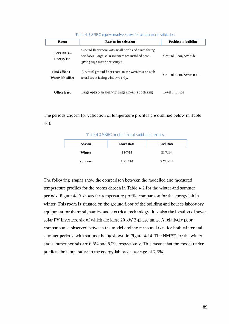
89
Table 4-2 SBRC representative zones for temperature validation.
Room Reason for selection Position in building
Flexi lab 3 –
Energy lab
Ground floor room with small north and south facing
windows. Large solar inverters are installed here,
giving high waste heat output.
Ground Floor, SW side
Flexi office 1 –
Water lab office
A central ground floor room on the western side with
small south facing windows only. Ground Floor, SW/central
Office East Large open plan area with large amounts of glazing Level 1, E side
The periods chosen for validation of temperature profiles are outlined below in Table
4-3.
Table 4-3 SBRC model thermal validation periods.
Season Start Date End Date
Winter 14/7/14 21/7/14
Summer 15/12/14 22/15/14
The following graphs show the comparison between the modelled and measured
temperature profiles for the rooms chosen in Table 4-2 for the winter and summer
periods. Figure 4-13 shows the temperature profile comparison for the energy lab in
winter. This room is situated on the ground floor of the building and houses laboratory
equipment for thermodynamics and electrical technology. It is also the location of seven
solar PV inverters, six of which are large 20 kW 3-phase units. A relatively poor
comparison is observed between the model and the measured data for both winter and
summer periods, with summer being shown in Figure 4-14. The NMBE for the winter
and summer periods are 6.8% and 8.2% respectively. This means that the model under-
predicts the temperature in the energy lab by an average of 7.5%.

90
Figure 4-13 SBRC energy lab temperature profile comparison – winter.
The indication of degree of correlation, R2, shows a poor result, with a very low
correlation between the model and the measured data for this room across both periods.
The scatter graph of the energy lab for the summer period is shown in Figure 4-15.
Figure 4-14 SBRC energy lab temperature profile comparison – summer.
The measured data for this room during both winter and summer periods appears to be
very erratic when compared to data from the other rooms considered here. One possible
cause of this may be due to the temperature sensor for the zone being located next to the
entrance door. An air exchange with the adjacent space, as well as possible air flow
across the temperature sensor caused by motion nearby each time the door is used may
be the cause of the erratic temperature behaviours seen here. The weekend period in
Figure 4-13 (from the 19/7/14) shows a moderately good correlation, albeit with some
offset error. The weekend period is one where very little activity takes place in this
room and thus the door is not used. This observation supports the theory that erratic
10
12
14
16
18
20
22
24
14/7/14 15/7/14 16/7/14 17/7/14 18/7/14 19/7/14 20/7/14 21/7/14
Inte
rnal
Tem
per
atu
re (
°C)
Energy Lab MEASURED
Energy Lab MODEL
10
12
14
16
18
20
22
24
26
28
15/12/14 16/12/14 17/12/14 18/12/14 19/12/14 20/12/14 21/12/14 22/12/14
Inte
rnal
Tem
per
atu
re (
°C)
Energy Lab MEASURED
Energy Lab MODEL

91
readings are caused by human movement between zones. This is one aspect that cannot
be considered by the model for two reasons:
i. The prediction of human behaviour is naturally very difficult to model
effectively due to its random nature. Long term surveys of every
entry/exit into and out of the zone may provide some insight that would
enable basic modelling of characteristic behaviour but this would be
beyond the scope of the modelling performed here;
ii. The temperature data output from the model is the average space
temperature recorded during the specified time interval. This makes it
impossible to detect the specific temperature recorded next to the
doorway as recorded by the sensor installed in reality.
A better outcome would be to change the way temperature is recorded in reality for this
zone. An average zone temperature would provide a better, more appropriate
comparison with the data output from the model, rather than the temperature at a single
point in the room, being susceptible to local effects.
Figure 4-15 R2 for energy lab room temperature comparison – summer.
Despite the less than ideal way in which temperature is measured for the zone, this is
unlikely to adversely affect the outcome of the modelling performed here. A visual
comparison of the temperature profiles shows similar general behaviour and an
acceptable NMBE for the periods examined.
The next room at the SBRC chosen for validation is the office adjacent to the water
laboratory on the ground floor. This room has east and south facing external walls and
R² = 0.1636
19
20
21
22
23
24
25
26
19 20 21 22 23 24 25 26
Mo
del
(°C
)
Measured (°C)
Energy lab - Model vs Measured

92
is regularly occupied by two to three people. The temperature profile comparison is
shown in Figure 4-16 for winter and Figure 4-18 for summer.
Figure 4-16 SBRC water lab office temperature profile comparison – winter.
When compared to that of the energy lab, the temperature profiles for this zone are
much more predictable and thus the model does a better job of determining its thermal
behaviour. The NMBE is calculated as 2.2% in winter and 4.1% in summer. The model
appears to underestimate temperatures in this zone. This is most evident over the
weekend, a time when no mechanical HVAC occurs, where a temperature difference of
approximate 1.5°C can be observed. The zone appears to lose heat faster overnight than
the real building once artificial heating has switched off.
Figure 4-17 R2 for water lab office room temperature comparison – winter.
The coefficient of determination of 64.3% is shown for the winter case in Figure 4-17.
As was discussed previously with regards to Figure 4-5, the horizontal streak of off-
trend data is due to the way the model idealises the HVAC response by maintaining the
zone at a constant setpoint. This is not the behaviour experienced in reality.
10
12
14
16
18
20
22
14/7/14 15/7/14 16/7/14 17/7/14 18/7/14 19/7/14 20/7/14 21/7/14
Inte
rnal
Tem
per
atu
re (
°C)
Water Lab Office MEASURED
Water Lab Office MODEL
R² = 0.643
15
16
17
18
19
20
21
22
23
15 16 17 18 19 20 21 22 23
Mo
del
(°C
)
Measured (°C)
Water lab office - Model vs Measured

93
Figure 4-18 SBRC water lab office temperature profile comparison – summer.
The zone behaviour in Figure 4-18 demonstrates that the building is in natural
ventilation mode in both the model and reality for the summer period. This is evident
through the fact that there are few rapid decreases in temperature that are consistent
with artificial cooling. The natural ventilation system is able to meet the cooling loads
for that particular week. Whilst the model does not follow the real data exactly, it is
considered a good result due to the fact that natural ventilation is rather difficult to
model with high accuracy. A 4.1% NMBE and an R2 value of 55.8% establishes a
satisfactory level of representation of the real building zone.
Figure 4-19 R2 for water lab office room temperature comparison – summer.
The temperature profile comparison of the eastern office for the winter period is shown
in Figure 4-20. This zone is at the eastern side of the building on the first floor. It is an
open plan office space which is serviced by two Variable Air Volume (VAV) boxes, as
well as a hydronic slab system. It is observed that the behaviour of the real building
10
12
14
16
18
20
22
24
26
15/12/14 16/12/14 17/12/14 18/12/14 19/12/14 20/12/14 21/12/14 22/12/14
Inte
rnal
Tem
per
atu
re (
°C)
Water Lab Office MEASURED
Water Lab Office MODEL
R² = 0.5576
19
20
21
22
23
24
25
26
19 20 21 22 23 24 25 26
Mo
del
(°C
)
Measured (°C)
Water lab office - Model vs Measured

94
does not follow that of the model, particularly during overnight periods. A NMBE of
7.7% is calculated and R2 is found to be 32.9%, as shown in Figure 4-21.
Figure 4-20 SBRC eastern office temperature profile comparison – winter.
As with previous scatter graphs, the horizontal streak of data shown at the top of Figure
4-21 is due to the way the model idealised HVAC performance and maintained
temperature at a constant level. With these data points excluded, R2 improves to 39.2%.
Figure 4-21 R2 for eastern office room temperature comparison – winter.
One possible cause of the disparity between temperature profiles in this zone is the
existence of the hydronic slab system. This system is scheduled to operate during the
summer and winter months, between the hours of 4:00AM and 6:00AM. During winter,
hot water is pumped through the slab, creating a slow release heat source designed to
reduce heating loads during the day. Cold water is used during summer, creating a slow
release heat sink.
0
5
10
15
20
25
14/7/14 15/7/14 16/7/14 17/7/14 18/7/14 19/7/14 20/7/14 21/7/14
Inte
rnal
Tem
per
atu
re (
°C)
Office East MEASURED
Office East MODEL
R² = 0.3288
15
16
17
18
19
20
21
22
23
15 16 17 18 19 20 21 22 23
Mo
del
(°C
)
Measured (°C)
Eastern Office - Model vs Measured

95
The hydronic system installed at the SBRC was not included in this model due to the
complexities of the HVAC system and the fact that the system in reality has not been
properly commissioned at this stage (though it does still operate). This would make it
difficult to model the system accurately when operating parameters (flow rates, fluid
temperatures, etc.) have not been properly defined. The omission of this system from
the model may explain why temperatures drop overnight by 3-4°C, while in the real
building temperatures remain much more stable throughout the working week.
The temperature comparison for the eastern office in summer is shown in Figure 4-22.
A NMBE of 3.95% is calculated. Whilst this appears to be a good result, the R2 for this
comparison is only 1%. There is almost zero correlation between the model and the
measured temperature profiles of the week.
Figure 4-22 SBRC eastern office temperature profile comparison – summer.
A possible reason for this could be that the building was in natural ventilation mode for
most of the week. Modelling of large, naturally ventilated spaces using this modelling
technique is unpredictable given various local weather effects that are not considered by
the weather file used in the simulations. Temperature profiles will not be a perfect
match and thus the R2 value may not be the best indicator of model success for this
case. A better result might have been achieved if the large open plan zone had been
modelled as several discrete thermal zones. The most important thing to consider is that
the model temperature profile remained within the comfort band of 20°C to 25°C during
occupied periods, which is indeed the case as shown in the figure.
Having compared the modelled temperature profiles for key building zones to the
measured profiles for a summer and winter representative week, it can be concluded that
the thermal performance of the building model is representative of the real building.
0
5
10
15
20
25
30
15/12/14 16/12/14 17/12/14 18/12/14 19/12/14 20/12/14 21/12/14 22/12/14
Inte
rnal
Tem
per
atu
re (
°C)
Office East MEASURED
Office East MODEL

96
Whilst the model cannot fully represent in detail the temperature response of a zone in
natural ventilation mode, the overall behaviour is considered to be accurate given that
the zones do stay within the natural ventilation comfort band. The hydronic slab system
has been ignored in this model due to it not being properly commissioned, as well as the
complexity it would add to the model. Given that such little definite data is available, it
would be very difficult to be able to quantify the energy implications of this system,
both how much energy use can be attributed to the hydronic system, as well as how
much of a net benefit it would have to HVAC energy consumption.
The validation of the energy aspects of the SBRC building model was hampered to an
extent by data availability. Data was available for the lighting, and IT systems up to
August 2014, and HVAC data for the entirety of 2014, however general plug loads and
building services loads are unavailable as these are metered separately and technical
difficulties prevented these meters from recording data. Additionally, 2014 was the
SBRC buildings first official year of occupation and thus commissioning processes to
building systems occurred during the early months of 2014, notably the HVAC system.
Nonetheless, enough data was available to provide some degree of confidence in the
model given that the most dominant building loads are represented by a sufficient
amount of data.
The energy profile comparison of the modelled lighting system with the real building
using daily lighting energy consumption is shown in Figure 4-23.
Figure 4-23 SBRC lighting electrical use comparison.
As described previously, the NMBE and the coefficient of variation of the root mean
squared error (CVRMSE) are used to describe the accuracy of the energy models - in
line with [73]. The NMBE and CVRMSE for the lighting model are -1.3% and 16.4%,
0
10
20
30
40
50
60
70
1/1/14 29/1/14 26/2/14 26/3/14 23/4/14 21/5/14 18/6/14 16/7/14
Dai
ly L
igh
tin
g lo
ad (
kWh
)
Lighting MEASURED
Lighting MODEL

97
respectively. This means that the model has overestimated the lighting loads by 1.0%.
The acceptable CVRMSE limit is set at 15% which suggests this model doesn’t quite fit
the data available. As with the TTT building model, it should be noted that the lighting
systems in these net-zero energy buildings are influenced by human behaviour and
external weather conditions, with occupancy and daylight sensors controlling their
operation. It is observed that on seven to ten occasions, the model underestimated the
lighting energy use for the week. This may have been due to higher than normal
occupancy or lower than normal natural light levels, perhaps caused by a run of days
with inclement weather.
Figure 4-24 shows the IT electrical load profile comparison for the SBRC building. A
NMBE was calculated as -0.3%, showing the model only slightly overestimated the IT
loads of the building. The CVRMSE is 3.7%, well below the 15% limit. This shows that
the IT model for the SBRC building is a good match. IT loads are one of the most easily
predicted, given the load profile is very flat and operates constantly. Since VDI
infrastructure is used at the SBRC, on-site IT loads are not highly influenced by
occupancy. Analysis of SBRC IT energy data reveals that IT loads increase by
approximately 300 W only during week days (the effect of occupancy) on top of a
1.5 kW base-load. The inaccuracies present in the model at the start of the validation
period can be explained by the building being commissioned during the first month of
2014.
Figure 4-24 SBRC IT electrical use comparison.
The HVAC profile comparison is shown below in Figure 4-25. The NMBE is calculated
as 2.7%, an acceptable value. However, the CVRMSE is 45.8%. This is far higher than
the 15% limit.
50
52
54
56
58
60
62
64
66
68
70
1/1/14 29/1/14 26/2/14 26/3/14 23/4/14 21/5/14 18/6/14 16/7/14
Dai
ly IT
load
(kW
h)
IT MEASURED
IT MODEL

98
Figure 4-25 SBRC HVAC electrical use comparison.
As with the TTT building HVAC model, the model for the SBRC did not consider
detailed system specifications. Rather, nominal system COP’s and auxiliary loads are
specified. The general operation of the HVAC system compares well on a larger
timescale, with the model showing the winter period being the time of highest HVAC
demand. The three peaks during the first three months of the year appear out of
character and these can be explained by the building still undergoing commissioning
during this time.
Having used historical weather data to compare the SBRC model simulations with real
measured temperature and energy data from the same period, it must be decided
whether the model is a satisfactory representation of the real SBRC building. Some
aspects of the model did not meet the error quantification metrics, particularly the
HVAC energy consumption. The temperature comparisons were a good fit overall with
the measured data, with inaccuracies coming from the complex and unpredictable
dynamics involved with natural ventilation, as well as the simplification of the model
HVAC system not incorporating the hydronic slab system. With these factors
considered, the thermal behaviour of the building was generally a good representation
of the SBRC building for the zones considered.
The comparisons of energy aspects of the model were generally acceptable for the data
that was available at the time. Whilst the HVAC model CVRMSE was three times
higher than the acceptable level, the general long term behaviour of the system
compared well with the measured data. There were too many unpredictable factors, as
well as technical modelling difficulties associated with the HVAC model, to make it
more accurate on shorter timescales.
0
50
100
150
200
250
300
350
400
1/1/14 10/2/14 22/3/14 1/5/14 10/6/14 20/7/14 29/8/14 8/10/14 17/11/14 27/12/14
Dai
ly H
VA
C lo
ad (
kWh
)
HVAC MEASURED
HVAC MODEL

99
The SBRC building model, despite the identified shortcomings, can be considered an
acceptable representation of the real building for the purposes intended in this study.
4.4.3 Enterprise 1
Metering capabilities at the Enterprise 1 building are less extensive than at the SBRC.
However, as the building has been operating for longer, more reliable data is available.
For this reason, it is possible to validate the Enterprise 1 building model using a full
year of energy data. Unfortunately, the energy model is only able to be validated against
the HVAC system and the combined light and power loads, as the lighting system and
all plug loads are metered together in the building. No separate data on IT is available.
Furthermore, temperature data for Enterprise 1 is not available. This is one difficulty
encountered when studying a more conventional commercial building. Due to the
SBRC and TTT being educational buildings, they have provision for research to take
place within them, meaning a deeper level of information is able to be obtained.
Enterprise 1, being a fully functioning commercial building, does not have this kind of
information available and organising to obtain it would require a potentially lengthy
planning and consultation process which could not be afforded by the timeline
constraining this research. However, that given the same modelling techniques were
used on the previous two buildings and that a good result was observed in those two
cases, it can be inferred with some confidence that the thermal behaviour of this
building is also acceptable.
The energy use comparison for the light and power systems is shown in Figure 4-26.
The NMBE is 1.7%, and the CVRMSE is 5.9%. These numbers are well within the
prescribed error limits. The model tends to reduce consumption from August onwards,
while in reality, the opposite trend appears to occur. Apart from this discrepancy, the
light and power comparison is a valid one.

100
Figure 4-26 Enterprise 1 light and power electrical use comparison.
The energy use comparison for the HVAC system at Enterprise 1 is shown in Figure
4-27. A good visual comparison is observed in general. A calculated NMBE of 2.8%
and CVRMSE of 21.7% confirmed that the HVAC model is the best representation out
of all three buildings. Reasons for this are that the Enterprise 1 HVAC system is more
conventional compared to the experimental systems installed in the SBRC and TTT
buildings. The occupancy of Enterprise 1 is also higher and steadier than at TTT and
SBRC which are educational buildings. This makes all electrical load profiles much
more predictable.
Figure 4-27 Enterprise 1 HVAC electrical use comparison.
Without a complete set of data for each separate building system, and temperature data
to ensure thermal behaviour is correct, it is difficult to say that the Enterprise 1 model is
a good representation of the real building. However, based on previous experience with
the other two buildings which were modelled with the same techniques, we can assume
with some confidence that the thermal behaviour of the Enterprise 1 model is accurate.
1000
1500
2000
2500
3000
3500
4000
1/1/14 15/2/14 1/4/14 16/5/14 30/6/14 14/8/14 28/9/14 12/11/14 27/12/14
Dai
ly L
igh
t an
d P
ow
er lo
ad (
kWh
)
Light and Power MEASURED
Light and Power MODEL
0
500
1000
1500
2000
2500
3000
1/1/14 15/2/14 1/4/14 16/5/14 30/6/14 14/8/14 28/9/14 12/11/14 27/12/14
Dai
ly H
VA
C lo
ad (
kWh
)
HVAC MEASURED
HVAC MODEL

101
Not being able to separate lighting and plug loads, it is difficult to say whether the
models for each individual building system are accurate on their own. It can be said
however, that combined, the model does a good job of correctly representing these loads
over an entire year. The same can be said for the HVAC system. Whilst the CVRMSE
is higher than the prescribed limit, it is the best performing HVAC model of all three
buildings.
It is with these issues in mind, that the Enterprise 1 building model can be said to be
valid for the purposes of the research conducted here.
4.4.4 Model limitations
Any model of an existing building can only be as good as the data and assumptions used
to verify it. For the three building models presented in this chapter, none of them had
complete energy data able to represent each typical season of the year. The TTT
building model was only able to be verified against energy data for summer and
autumn. Whilst the SBRC and Enterprise 1 models had the advantage of having a full
year of mechanical HVAC data, other aspects of energy use were missing or were not
individually metered in the first instance. Where incomplete data is a reality, reasonable
assumptions must be relied on based on typical benchmark values and technical
building information. While light and power were lumped into one meter at the
Enterprise 1 building, making it difficult to validate the lighting model on its own,
reviewing the technical documentation on the lighting system in the real building
enabled correct sizing of the system in the model. Whilst simulation results cannot be
directly compared to metered building data, the assumptions used are able to be relied
upon. Some assumptions are more reliable than others and depend on the accuracy of
the information upon which they are based.
The validation process of efficient building models presents challenges less common for
models of more conventional buildings. Highly automated systems associated with
efficient buildings makes energy consumption less predictable as it is based on a higher
number of variables not necessarily accounted for by the model.
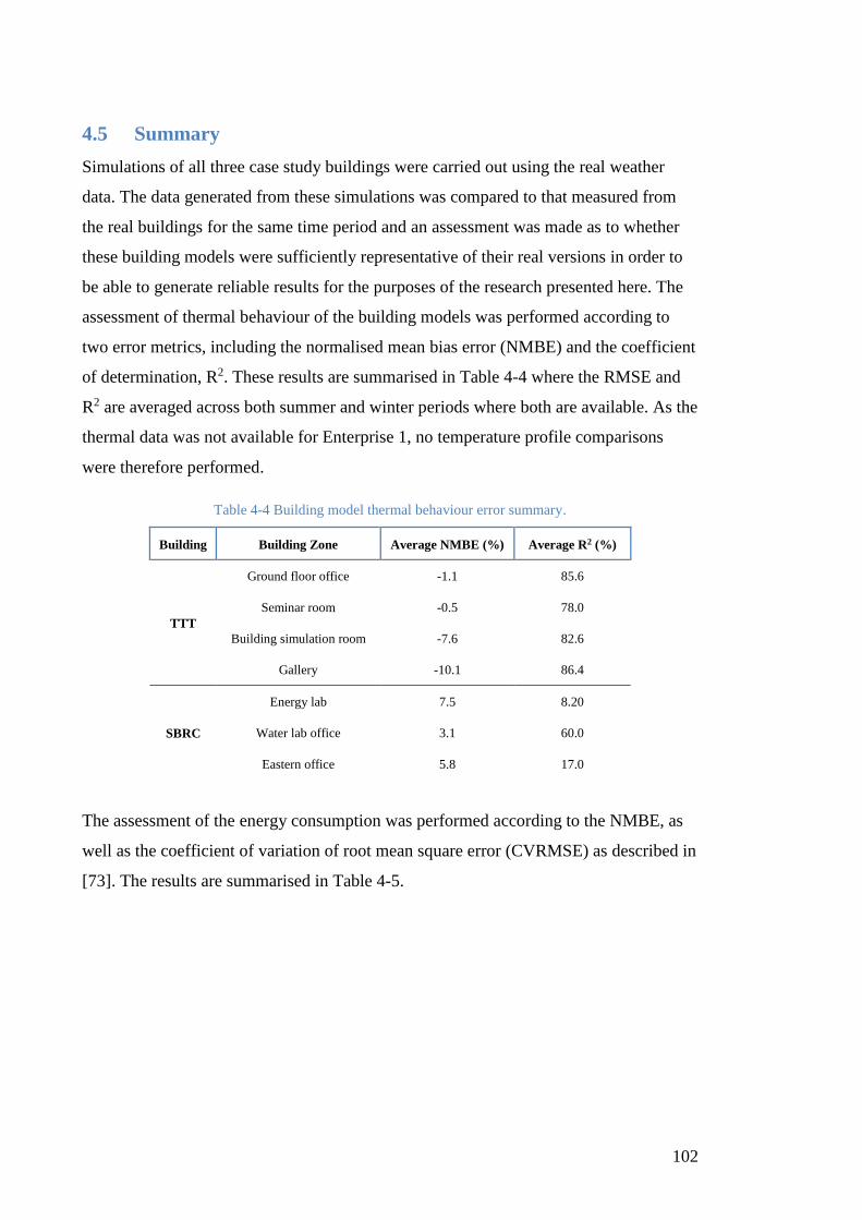
102
4.5 Summary
Simulations of all three case study buildings were carried out using the real weather
data. The data generated from these simulations was compared to that measured from
the real buildings for the same time period and an assessment was made as to whether
these building models were sufficiently representative of their real versions in order to
be able to generate reliable results for the purposes of the research presented here. The
assessment of thermal behaviour of the building models was performed according to
two error metrics, including the normalised mean bias error (NMBE) and the coefficient
of determination, R2. These results are summarised in Table 4-4 where the RMSE and
R2 are averaged across both summer and winter periods where both are available. As the
thermal data was not available for Enterprise 1, no temperature profile comparisons
were therefore performed.
Table 4-4 Building model thermal behaviour error summary.
Building Building Zone Average NMBE (%) Average R2 (%)
TTT
Ground floor office -1.1 85.6
Seminar room -0.5 78.0
Building simulation room -7.6 82.6
Gallery -10.1 86.4
SBRC
Energy lab 7.5 8.20
Water lab office 3.1 60.0
Eastern office 5.8 17.0
The assessment of the energy consumption was performed according to the NMBE, as
well as the coefficient of variation of root mean square error (CVRMSE) as described in
[73]. The results are summarised in Table 4-5.

103
Table 4-5 Building model energy use error summary.
Building Building system Average NMBE (%) Average CVRMSE (%)
TTT
Lighting 12.5 38.4
General Power 5.9 18.1
HVAC 12.2 50.1
SBRC
Lighting -1.3 16.4
IT -0.3 3.7
HVAC 2.7 45.8
Enterprise 1
Lighting and power 1.7 5.9
HVAC 2.8 21.7
It was only possible to work with the datasets available and as such, although validated
model summaries for each building appear together in the same tables, this should not
be taken to mean that consistent and perfectly corresponding periods of data were used
to validate each building. Data used (where it was available) came from varying time
periods. It cannot be said that every building was validated according to data occurring
at the same time.
Overall, the Enterprise 1 building model appears to perform the best when viewing the
numbers, however it is also the building with the least extensive metering and thus only
two building systems were able to be assessed against the validation methodology.
Building size has an effect on the accuracy of the models. A larger building is less
sensitive to random events that may affect energy consumption. These events are those
dictated by human activity such as an occupant opening a window or turning on lights.
Each occupant has differing preferences for thermal and visual comforts. In smaller
buildings which have less than 50 regular occupants, such as the SBRC and TTT
buildings, random events linked to occupant behaviour have more influence on energy
consumption of building systems. The effect of occupants preferring to have a window
open in Enterprise 1 for example, will have lesser effect on overall HVAC energy
consumption than it would at the SBRC. This is one reason why the Enterprise 1 model
achieved a better validation result than the other smaller buildings. Other reasons for
this may be that the occupancy rate and schedules are more regular due to Enterprise 1
being a commercial building, whilst the other two buildings are for educational

104
purposes. These buildings have variable occupancy rates and times depending on
timetabling and other special events. This makes the behaviour of Enterprise 1 much
easier to predict in the model, thus further reducing error.

105
Chapter 5 Simulation Results and Discussion
5.1 Simulation Results
By performing simulations of all three buildings using the validated models in
DesignBuilder, an understanding into the sensitivity of each building to changes in
design and construction from the point of view of energy consumption can be gained.
From this understanding, better informed decisions can be made when designing a
NZEB or considering upgrades to existing buildings in order to improve energy
efficiency. It is important when viewing the changes in energy consumption of one
building system, that its contribution to overall building energy use is considered. After
all, in most circumstances the end goal is to reduce overall building consumption, not
just the consumption of one system if, consequently consumption by another system
may rise. The energy use breakdown (EUB) for each building is shown below in Figure
5-1. The data used to create these EUB’s is the data generated from the model outputs.
Due to metering complications and inconsistencies between buildings, complete and
consistent metered data could not be used to form real-world EUB’s. However, as the
models are representative of the real buildings, the EUB’s generated are also
representative of reality. Indeed, the data that was available compares well to the
modelled EUB’s where comparison was possible.
Figure 5-1 Energy Use Breakdown of three case study buildings.
From Figure 5-1 it is observed that the two NZEBs are very similar in their EUB, with
lighting being the smallest component, and HVAC being roughly 50% of overall loads.
On the other hand, the HVAC load at Enterprise 1 is the smallest component, making up
only one quarter of overall loads. This means that different outcomes will be expected
54.4%
49.4%
25.4%
17.0%
19.4%
35.6%
28.6%
31.2%
39.0%
0% 20% 40% 60% 80% 100%
TTT
SBRC
Enterprise 1
HVAC Lighting IT and General

106
for overall energy use between the NZEB and conventional building when effects on
HVAC energy use are significant.
5.1.1 Glazing
With the windows of a building needing to serve as both a visual connection to the
outdoors, and an impermeable barrier to the outdoor elements, they form a critically
important contribution to a well performing building envelope. The type of glazing used
in a building can affect energy consuming building systems. Different window designs
will let different amounts of sunlight into the building. This has consequences for how
much artificial light is needed to sufficiently illuminate the building. Windows also
allow heat to pass through them as well as visible light. Due to their transparent nature,
high levels of conventional insulation are not possible in windows as they are with
walls. The highest rates of heat transfer per m2 through a building envelope typically
take place through the windows [34]. For a building with a high window to wall ratio,
this can mean significant overall heat loss occurs through the building envelope. The
result of this is that HVAC loads are increased and energy consumption is driven up.
Whilst having more windows may mean that lighting energy consumption may come
down, it is likely that HVAC energy consumption will increase. It is this balance that
will be better understood by simulation of the test cases.
Before detailed modelling results are outlined, it is important to ensure window
performance terminology is correctly understood. Solar Heat Gain Coefficient (SHGC)
is a measure of how well the radiant energy from sunlight is transferred through the
window and thus adds heat to the space. It is defined as the fraction of incident solar
radiation transferred through glass (sometimes is it specified as the glass and frame) and
is expressed as a number between 0 and 1 [81]. A higher SHGC will potentially allow
more heat to pass into the internal space. This may have benefits in a colder climate, and
certainly has disadvantages in warmer climates.
Visible transmittance is a measure of how much daylight passes through the window
and is also expressed as a number between 0 and 1. A higher number means more light
is transmitted. This parameter concerns only light in the visible spectrum.
U-value (otherwise known as thermal conductance) is a measure of how well the
window conducts heat. The U-value is used to specify many other types of building
materials and is the inverse of the R-value, the parameter commonly used to specify the

107
performance of insulation materials. U is specified in units of W/m2-K. In other words,
it is the rate of heat transfer per unit area, per unit Kelvin temperature difference. The U
value may apply to both glass/air gap and frame, or glass/air gap only. Here, it applies
to the glass/air gap only. The window frames used throughout all scenarios in this study
are consistent and thus the specifications of the SHGC and U-value as being ‘glass-
only’ should not adversely affect the analysis. The frame type is aluminium with
thermal break.
Table 5-1 shows the glazing specifications for all simulated scenarios for all three
buildings. A predictable downward trend is observed in most parameters as glazing
scenarios progress toward the highest performance option (LowE triple glazed). Note
however that Double LowE glazing performs better than regular triple glazing for
SHGC.
Table 5-1 Glazing simulation scenarios.
Glazing
Scenario Glass Type (Layer 1/2/3)
Glass
Thickness
(mm)
Air Gap
(mm) SHGC
Visible
Transmittance
U-Value
(W/m2-
K)
Single Generic Clear 6 - 0.819 0.881 5.778
Single
LowE Generic PYR B Clear 6 - 0.72 0.811 3.779
Double Generic Clear 6 13 0.703 0.781 2.665
Double
LowE Generic LowE/PYR B Clear 6 13 0.634 0.721 1.931
Triple Generic Clear 3 13 0.684 0.738 1.757
Triple
LowE
Generic LowE Clear/Generic
Clear/Generic LowE 3 13 0.474 0.661 0.982
Building envelope parameters for each test case are summarised in Table 5-2. The ratios
of window area to both floor and external wall area are also given. The window to floor
ratio remains consistent across all three buildings with an average value of 0.229. When
the high bay wing of the SBRC is excluded, these numbers change significantly. The
high bay wing is a large 900 m2 area which is naturally ventilated only, and is designed
with very low lighting loads. As a result, it has a very low energy impact on HVAC and
lighting systems. The window to floor ratio at the SBRC with the high bay wing

108
excluded becomes 0.357, the highest of all three buildings. The Window to Wall Ratio
(WWR) when the high bay wing is excluded becomes 0.436, up from 0.288 when the
high bay is considered. This is still lower than the WWR of Enterprise 1, which is
0.710.
Table 5-2 Case study building envelope parameters.
Building Floor Area
(m2)
Window Area
(m2)
Wall Area
(m2)
Window to Wall
Ratio
Window to Floor
Ratio
TTT 1021 218 813 0.268 0.214
SBRC 2600 652 2261 0.288 0.251
SBRC (ex HB) 1700 606 1390 0.436 0.357
E1 11874 2649 3730 0.710 0.223
The simulations performed were conducted over a period of an entire year. The
simulation time interval is 1 hour. The results are compared to the single glazed
scenario which, in this case is treated as the benchmark. Single glazing is not installed
in the real case-study buildings, however as glazing technology in each real building
varies, it is easier to compare each building to a common benchmark. Figure 5-2 shows
the per cent change in yearly HVAC energy use for each glazing technology across all
three buildings. As is expected, as glazing performance increases, HVAC loads decrease
as a response to the reduced SHGC and U-value. It is noted that there is a small increase
in energy use between the double glazed LowE option and the triple glazed clear option
for all buildings. This indicates that a double-glazed option with low emissivity glass is
a better choice than triple glazing in this case.
It is clear that the HVAC energy savings at the SBRC are higher than at the other
buildings. This gap widens as glazing performance increases, with HVAC energy
reduction at the SBRC occurring at a higher rate than with the other buildings.

109
Figure 5-2 Glazing simulations: change in HVAC energy use.
The per cent change in lighting energy use for the three buildings across a full year is
shown in Figure 5-3. The opposite behaviour to that seen in Figure 5-2 is observed. This
is expected, since a higher performing window will typically reduce solar heat gains at
the expense of also reducing visible light. Again, the difference between double glazed
LowE and triple glazed clear is the opposite of the overarching trend. The magnitude of
the change in lighting energy use at the SBRC building is much higher and increases at
a higher rate than for the other two buildings. This is the same trend seen in Figure 5-2,
but the effect is much more pronounced.
Figure 5-3 Glazing simulations: change in lighting energy use.
When the data from Figure 5-2 and Figure 5-3 is combined, the overall effect of
different glazing technologies on total building energy consumption for the year is
shown in Figure 5-4. Clearly the overall effect of higher performance glazing on total
building energy use across a whole year is a net reduction in energy use for the three
buildings studied. The building that benefits most from high performance glazing is the
-25.0%
-20.0%
-15.0%
-10.0%
-5.0%
0.0%
Single LowE Double Double LowE Triple Triple LowE
Ch
ange
in H
VA
C e
ner
gy u
se (
%)
Glazing type
SBRC TTT Enterprise 1
0.0%
2.0%
4.0%
6.0%
8.0%
10.0%
12.0%
Single LowE Double Double LowE Triple Triple LowE
Ch
ange
in li
ghti
ng
ener
gy u
se (
%)
Glazing type
SBRC TTT Enterprise 1

110
SBRC, with the TTT building experiencing the second highest saving. It appears that
when choosing between double glazed LowE windows and triple glazed clear, the
highest performing window technology is double glazed LowE by a small margin.
Figure 5-4 Glazing simulations: change in total building energy use.
The benefits to Enterprise 1 of high performing glazing technology are noticeable, but
to a much smaller degree than the other two buildings. Whilst a maximum of 11%
reduction in HVAC energy use and maximum 1.1% increase in lighting loads was
predicted at Enterprise 1, a review of Figure 5-1 illustrates that the lighting energy use
at Enterprise 1 represents a significantly larger portion of overall energy than that of the
HVAC system. The overall net effect on the building is a 1.9% reduction in overall
energy use.
To better understand why the SBRC building energy consumption may be more
sensitive to changes in glazing technology, a separate set of simulations was performed
where the lighting systems were identical. The lighting power density of all zones in all
buildings was set at 5 W/m2.
-12.00%
-10.00%
-8.00%
-6.00%
-4.00%
-2.00%
0.00%
Single LowE Double Double LowE Triple Triple LowE
Ch
ange
in b
uild
ing
ener
gy u
se (
%)
Glazing type
SBRC TTT Enterprise 1

111
Figure 5-5 Glazing simulations: change in HVAC energy use for identical LPD.
Figure 5-5 and Figure 5-6 show the results of the simulations with identical lighting
power densities. The effects on lighting energy (Figure 5-6) show the same trend as was
observed previously. The increase in lighting energy consumption for the SBRC
building is far higher than for the other two buildings. In fact, for an increased LPD of
5 W/m2 (the actual LPD at the SBRC is 1.6 W/m2), the change in energy consumption
increases.
Figure 5-6 Glazing simulations: change in lighting energy use for identical LPD.
By simulating all three buildings with identical lighting power densities, it can be
concluded that lighting system design is not the significant driving factor behind a
building’s energy sensitivity to reduced natural lighting levels caused by higher
performance glazing.
To better understand what could be the driving factor in the results seen in the previous
figures, data concerning the frequency of lighting system operation was analysed. For
the SBRC and TTT buildings, the lighting system is controlled by occupancy and
-30.0%
-25.0%
-20.0%
-15.0%
-10.0%
-5.0%
0.0%
Single LowE Double Double LowE Triple Triple LowE
Ch
ange
in H
VA
C e
ner
gy u
se (
%)
Glazing type
SBRC (LPD=5) TTT (LPD=5) Enterprise 1 (LPD=5)
0.0%
2.0%
4.0%
6.0%
8.0%
10.0%
12.0%
14.0%
16.0%
Single LowE Double Double LowE Triple Triple LowE
Ch
ange
in li
ghti
gn e
ner
gy u
se (
%)
Glazing type
SBRC (LPD=5) TTT (LPD=5) Enterprise 1 (LPD=5)

112
daylight sensors. If the zone is sensed as being occupied, the lighting system is able to
operate. The daylight sensors determine how much light, if any, needs to be provided by
the artificial lighting system.
To investigate the cause of the higher magnitude of increase in lighting energy at the
SBRC, the average full load hours per week as a percentage of the total scheduled hours
per week was graphed for both TTT and SBRC. Enterprise 1 does not have full
daylighting control and thus the values for this building would be at 100% for all cases.
The lighting systems in the models are controlled by a schedule. This is the best way of
approximating occupancy in each zone. Whilst in reality, occupancy is a random
phenomenon; it is in most cases, regular and predictable to a reasonable degree of
accuracy. The average full load hours per week are the average number of hours for
each zone where the lighting system is operating at 100% of its output potential (i.e. no
dimming). The daylighting control enables the lighting system to dim to 20%. An
increase in the number of hours operating at 100% would indicate lower natural light
levels on average.
Figure 5-7 shows the full load lighting hours per week as a percentage of the total
scheduled hours for both the SBRC and TTT building models. This term shall be known
as the lighting utilisation rate. Whilst the TTT building shows a small increase in
lighting utilisation of less than 1% across the glazing performance spectrum, the SBRC
experiences a much larger increase of more than 4% across the glazing performance
spectrum. This means that the SBRC adaptive lighting system is more sensitive to
changes in daylight levels compared to the TTT adaptive lighting system.

113
Figure 5-7 Glazing simulations: lighting system average weekly utilisation rates.
One likely reason for the SBRC building being more sensitive to variable daylight
levels is building layout. Figure 5-8 shows the layout of the first floor of the TTT
building. The first floor represents the majority of the building occupied floor area.
Figure 5-8 TTT building level 1 floor plan [82].
The SBRC building layout (shown in Figure 5-9) in comparison to the TTT building is
much narrower in width in its two wings. The longest dimension is that running east-
west. This results in an aspect ratio (the ratio of the longest dimension to shortest
dimension) for each wing at the SBRC of approximately 4:1. The aspect ratio at the
TTT is approximately 1.2:1 for the western portion of the building where most building
activity and energy consumption takes place.
50.0%
51.0%
52.0%
53.0%
54.0%
55.0%
56.0%
57.0%
58.0%
59.0%
60.0%
Single Single LowE Double Double LowE Triple Triple LowE
Ligh
tin
g av
g. w
eekl
y u
tilis
atio
n (
%)
Glazing type
SBRC TTT
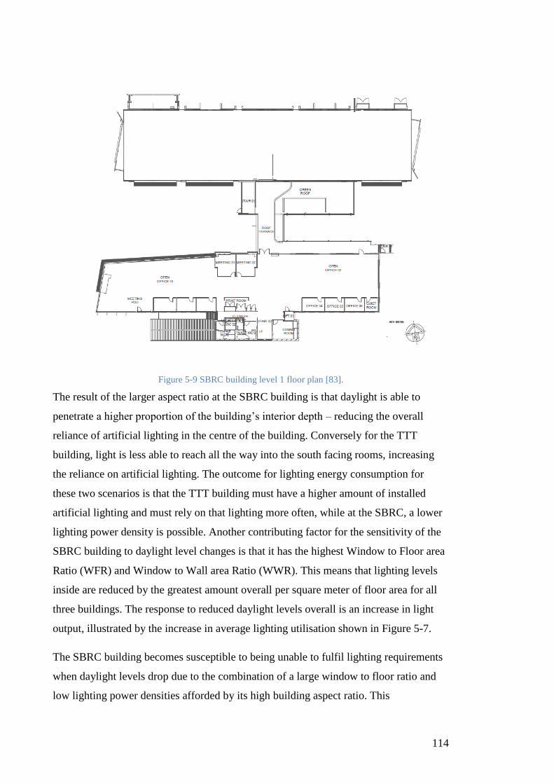
114
Figure 5-9 SBRC building level 1 floor plan [83].
The result of the larger aspect ratio at the SBRC building is that daylight is able to
penetrate a higher proportion of the building’s interior depth – reducing the overall
reliance of artificial lighting in the centre of the building. Conversely for the TTT
building, light is less able to reach all the way into the south facing rooms, increasing
the reliance on artificial lighting. The outcome for lighting energy consumption for
these two scenarios is that the TTT building must have a higher amount of installed
artificial lighting and must rely on that lighting more often, while at the SBRC, a lower
lighting power density is possible. Another contributing factor for the sensitivity of the
SBRC building to daylight level changes is that it has the highest Window to Floor area
Ratio (WFR) and Window to Wall area Ratio (WWR). This means that lighting levels
inside are reduced by the greatest amount overall per square meter of floor area for all
three buildings. The response to reduced daylight levels overall is an increase in light
output, illustrated by the increase in average lighting utilisation shown in Figure 5-7.
The SBRC building becomes susceptible to being unable to fulfil lighting requirements
when daylight levels drop due to the combination of a large window to floor ratio and
low lighting power densities afforded by its high building aspect ratio. This
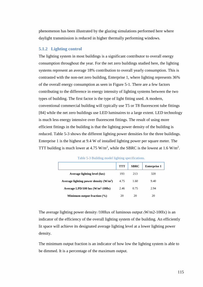
115
phenomenon has been illustrated by the glazing simulations performed here where
daylight transmission is reduced in higher thermally performing windows.
5.1.2 Lighting control
The lighting system in most buildings is a significant contributor to overall energy
consumption throughout the year. For the net zero buildings studied here, the lighting
systems represent an average 18% contribution to overall yearly consumption. This is
contrasted with the non-net zero building, Enterprise 1, where lighting represents 36%
of the overall energy consumption as seen in Figure 5-1. There are a few factors
contributing to the difference in energy intensity of lighting systems between the two
types of building. The first factor is the type of light fitting used. A modern,
conventional commercial building will typically use T5 or T8 fluorescent tube fittings
[84] while the net zero buildings use LED luminaires to a large extent. LED technology
is much less energy intensive over fluorescent fittings. The result of using more
efficient fittings in the building is that the lighting power density of the building is
reduced. Table 5-3 shows the different lighting power densities for the three buildings.
Enterprise 1 is the highest at 9.4 W of installed lighting power per square meter. The
TTT building is much lower at 4.75 W/m2, while the SBRC is the lowest at 1.6 W/m2.
Table 5-3 Building model lighting specifications.
TTT SBRC Enterprise 1
Average lighting level (lux) 193 213 320
Average lighting power density (W/m2) 4.75 1.60 9.40
Average LPD/100 lux (W/m2-100lx) 2.46 0.75 2.94
Minimum output fraction (%) 20 20 20
The average lighting power density /100lux of luminous output (W/m2-100lx) is an
indicator of the efficiency of the overall lighting system of the building. An efficiently
lit space will achieve its designated average lighting level at a lower lighting power
density.
The minimum output fraction is an indicator of how low the lighting system is able to
be dimmed. It is a percentage of the maximum output.

116
The type of light fitting is not the only contributor to reduced lighting power density.
Notice also in Table 5-3, the average lighting level in the building varies too. The
lighting system at Enterprise 1 is specified at 320 lx according to Australian standard
AS 1680 [85]. A 320 lux is recommended for “routine office work”. The two net zero
buildings have much lower average lighting levels. This is because whatever deficit
there may be in overall lighting levels, localised, low power light sources are utilised on
work surfaces to ensure lighting levels are appropriate. This enables much lower
lighting power densities. Additionally, the increased reliance on daylighting in the net
zero buildings contribute to the lower lighting power densities in those buildings.
Simulating building scenarios where different output light fittings are used could be
performed. However, the result is quite predictable without having to perform whole-
building energy simulations. A reduction in power consumption of each fitting is
relatively constant, and thus it would be possible to calculate with reasonable accuracy,
any overall consumption differences if the basic lighting specifications of each building
are known. What is more interesting, and more appropriate to simulate, is lighting
output control based on available daylight levels. This is a much more complex system
and depends on many variables such as building design and construction, as well as
weather conditions.
Each building model was simulated with and without a daylight-controlled lighting
system. The results were compared below; Figure 5-10 shows the lighting energy use
intensity across an entire year for each building. Lighting energy use intensity
(kWh/mfloor2) is the metric used here to enable practical comparison on one graph due to
the significant differences in overall energy use across the three buildings. The results
show that the energy use attributed to lighting can be reduced by between 49 and 65%.
Enterprise 1 would benefit greatly from daylighting control because of its high window
to wall ratio. An older style of conventional building may not respond as well to this
type of lighting control since daylight may not as readily reach into the centre of the
building. Enterprise 1 office space is centred on a heavily lit atrium area with large
skylights that would convey a large amount of daylight into the space.

117
Figure 5-10 Lighting control simulations: yearly lighting energy use intensity.
The effect on the HVAC system from daylight controlled lighting is show in Figure
5-11. Overall, there is a saving as a result of reduced lighting use resulting in less waste
heat output. The Enterprise 1 building model predicts the biggest saving of the buildings
with a 10% reducing in HVAC energy use intensity. Much of this saving can be
attributed to the waste heat from fluorescent lights being reduced. This saving is less
significant in the other two buildings because the more efficient lighting technology
used there does not emit as much waste heat. Savings in HVAC energy use intensity for
the net zero buildings are between 2% and 5 %.
Figure 5-11 Lighting control simulations: yearly HVAC energy use intensity.
Considering the effects on lighting and HVAC energy consumption, the net effect on
overall building energy consumption was compared between the three buildings. Figure
5-12 shows the yearly building energy use intensity for each building. The results show
that the Enterprise 1 building would have the greatest net benefit from daylight controls
with a very significant 25% reduction in overall building energy use. The TTT
0
10
20
30
40
50
60
70
TTT SBRC Enterprise 1
Ener
gy in
ten
sity
(kW
h/m
2 )
Control ON Control OFF
0
5
10
15
20
25
30
TTT SBRC Enterprise 1
Ener
gy in
ten
sity
(kW
h/m
2 ) Control ON Control OFF

118
simulation suggests that the building experiences a 21% overall energy saving as a
result of daylight controls. The smallest impact is seen at the SBRC where only 8% of
energy savings can be attributed to daylight controls.
Figure 5-12 Lighting control simulations: yearly building energy use intensity.
The reason daylight controls at the SBRC contribute to such a small overall saving is
that the installed lighting power density is so low because of the building being
optimised to take advantage of maximum daylighting levels. It is a different story at the
TTT where a higher provision of artificial lighting is installed. Whilst it is a NZEB, the
installed lighting power density is three times higher than at the SBRC because of the
lower aspect ratio and its implications for daylighting as described previously in Section
5.1.1.
5.1.3 Window shading
There are many potential techniques and design principles that may be applied to the
shading of a building. Primarily the purpose of shading, no matter how it is applied, is
to reduce the cooling loads in a building and to optimise the quality of daylight entering
the interior of the building by controlling glare levels. For these reasons, it comes as no
surprise that incorporation of shading elements is of critical importance to net zero
energy building design. Shading can be implemented in a number of ways. Some of
these are integral to the building’s design and construction, such as a roof overhang,
which must be designed to maximise the transmission of low winter sun, while
minimising the transmission of high winter sun. Other techniques are incorporated into
the building envelope such as vertical or horizontal louvres placed in front of a
window’s external face. These building-integrated shading approaches require a high
degree of knowledge of building design principles, as well as information about the
0
20
40
60
80
100
120
140
TTT SBRC Enterprise 1
Ener
gy in
ten
sity
(kW
h/m
2 ) Control ON Control OFF

119
building site, such as nearby structures, landmarks, vegetation and building orientation.
A simpler approach to shading is simply implementing shading of windows using blinds
or curtains. These are typically controlled by occupants to suit their personal tastes and
comfort requirements. Window shading may also be effective in some cases at reducing
energy consumption.
For the purposes of this study, simulation of local, building-integrated shading will be
ignored due to the need for it to be designed specifically according to the building and
its location. This would make it difficult to compare results between the case study
building models. Horizontal slatted blinds will be investigated instead. A common type
of window shading and a common control method across all buildings will be easily
comparable. The blind type used in this study is a blind with high reflectivity slats
which is provided as a default in the DesignBuilder library. A description of each
control strategy modelled is given in Table 5-4.
Table 5-4 Shading simulation control strategies.
Shading Control
Strategy Description
Summer day Blinds closed between 7:00 and 19:00 for all summer days (from 1st Dec to 28th Feb)
Summer night Blinds closed between 19:00 and 7:00 for all summer nights (from 1st Dec to 28th Feb)
Winter day Blinds closed between 7:00 and 19:00 for all winter days (from 1st June to 31st Aug)
Winter night Blinds closed between 19:00 and 7:00 for all winter nights (from 1st June to 31st Aug)
Temperature 26°C Blinds closed when outdoor temperature is above 26°C at all times of the day
Temperature 28°C Blinds closed when outdoor temperature is above 28°C at all times of the day
Temperature 30°C Blinds closed when outdoor temperature is above 30°C at all times of the day
Temperature 32°C Blinds closed when outdoor temperature is above 32°C at all times of the day
The window shading implemented here in this study does not replace any building
integrated shading elements in the original design. Some degree of shading is present in
each test case in the form of roof overhangs, window louvres, or both. These are left as-

120
designed in the building models. The window shading studied here is in addition to the
originally designed and built-in shading elements of the building envelope. The results
are compared to a benchmark where these local shading elements do exist, but where no
window shading is used.
The change in lighting energy use because of window shading controlled according to
the season is given in Figure 5-13.
Figure 5-13 Shading simulations: lighting energy use, seasonal schedule.
Unsurprisingly, the result is an increase in lighting use when shading is implemented
during the day for both summer and winter. The SBRC building model appears most
sensitive in summer, while Enterprise 1 is the least sensitive. Both the TTT and SBRC
experience a similar degree of change for the winter daytime case. Since all three
buildings are primarily occupied only during the daytime, only small changes were seen
for the summer and winter night time control cases.
The lighter colour, patterned columns on the graph represent the per cent change in
lighting energy use in proportion to the window to floor area ratio. Whilst this is not
necessarily a useful metric with which to specify a building or lighting design by, it is a
nominal dimension which does give an indication of the comparative sensitivity of the
buildings to window shading. From the graph, the comparative magnitudes of these
values are largely similar to those of the absolute change in lighting energy use. This
indicates that the WFR is likely to be the determining factor in the degree of change in
energy consumption for the lighting system. To make sure of this, the per cent change in
lighting energy use is also compared to the window area on its own. This is shown in
0.0%
4.0%
8.0%
12.0%
16.0%
20.0%
24.0%
28.0%
32.0%
36.0%
40.0%
0.0%
1.0%
2.0%
3.0%
4.0%
5.0%
6.0%
7.0%
8.0%
9.0%
10.0%
Summer Day Winter Night Summer Night Winter Day
Ch
ange
in li
ghti
ng
ener
gy u
se/W
FR (
%)
Ch
ange
in li
ghti
ng
ener
gy u
se (
%)
Control schedule
SBRC TTT E1
SBRC_WFR TTT_WFR E1_WFR

121
Figure 5-14. When compared to window area alone, the units are multiplied by a factor
of 1,000 to scale the values up due to window areas being much larger than the per cent
change in energy.
Figure 5-14 Shading simulations: change in lighting energy/Awindow - seasonal.
A different behaviour is observed when the per cent change/window area (Awindow) is
examined. The TTT building experiences a larger per cent change / area of window than
that of the SBRC and Enterprise 1 models. This makes sense since it has the smallest
total window area of the three buildings.
Comparing the change in HVAC energy use as a result of shading according to a
seasonal control strategy, Figure 5-15 shows that similar behaviour was observed as in
Figure 5-13 but with reversed changes, the HVAC loads decrease during the summer
day due to a cut in heat gain through the windows. Little change is observed for the
summer and winter night time control strategies, but interestingly HVAC energy use
increases for the case where shading is implemented during winter days. This is because
solar heat gain through windows helps to reduce heating loads during these periods. The
TTT building benefits most from this effect since the HVAC energy use increases by
16% when solar gains are reduced through shading. At the SBRC, HVAC energy use
increases by only 8%. Little change is observed for Enterprise 1.
0.0%
4.0%
8.0%
12.0%
16.0%
20.0%
24.0%
28.0%
32.0%
36.0%
40.0%
0.0%
1.0%
2.0%
3.0%
4.0%
5.0%
6.0%
7.0%
8.0%
9.0%
10.0%
Summer Day Winter Night Summer Night Winter Day
Ch
ange
in li
ghti
ng
ener
gy u
se/A
w
(10
00
*[%
/m2 ]
)
Ch
ange
in li
ghti
ng
ener
gy u
se (
%)
Control schedule
SBRC TTT E1
SBRC_Aw TTT_Aw E1_Aw

122
Figure 5-15 Shading simulations: HVAC energy - seasonal schedule.
Once again, comparing the change in energy use/window to floor area ratio, with the
change in energy use/window area gives some indication of what the determining
parameter is with regards to the buildings’ sensitivity to shading levels. The change in
energy use/window area is shown in Figure 5-16. The behaviour observed is similar to
that in Figure 5-14, where the TTT building appears to experience the largest per cent
change in HVAC energy use per m2 of window area.
Figure 5-16 Shading simulations: change in HVAC/Awindow - seasonal schedule.
It is not until the relationship between floor area and window area is considered, that it
becomes clear that this parameter is closely aligned with the relative changes in energy
use for both lighting and HVAC.
-40.0%
-32.0%
-24.0%
-16.0%
-8.0%
0.0%
8.0%
16.0%
24.0%
32.0%
40.0%
-10.0%
-8.0%
-6.0%
-4.0%
-2.0%
0.0%
2.0%
4.0%
6.0%
8.0%
10.0%
Summer Day Winter Night Summer Night Winter Day
Ch
ange
in H
VA
C e
ner
gy u
se/W
FR (
%)
Ch
ange
in H
VA
C e
ner
gy u
se (
%)
Control schedule
SBRC TTT E1
SBRC_WFR TTT_WFR E1_WFR
-40.0%
-32.0%
-24.0%
-16.0%
-8.0%
0.0%
8.0%
16.0%
24.0%
32.0%
40.0%
-10.0%
-8.0%
-6.0%
-4.0%
-2.0%
0.0%
2.0%
4.0%
6.0%
8.0%
10.0%
Summer Day Winter Night Summer Night Winter Day
Ch
ange
in lH
VA
C e
ner
gy u
se/A
w
(10
00
*[%
/m2])
Ch
ange
in lH
VA
C e
ner
gy u
se (
%)
Control schedule
SBRC TTT E1
SBRC_Aw TTT_Aw E1_Aw

123
The changes in lighting and HVAC energy for window shading using a temperature
threshold control strategy are shown in Figure 5-17 and Figure 5-18. What is most
obvious is that the biggest changes come from lower temperatures, with the largest
effect being seen at the SBRC for both lighting and HVAC. The increase in lighting
energy at the TTT and Enterprise 1 were of similar magnitude of around 1.5%, while
the decrease in HVAC energy at the TTT compares more closely with the SBRC at
around 3.6 to 4.8%.
Figure 5-17 Shading simulations: lighting energy use - temperature control.
Interestingly, changes in energy consumption decrease as the threshold temperature for
implementing shading increases. The minimum temperature of 26°C is chosen as being
just above the cooling setpoint temperature for each of the three buildings.
Temperatures below this would interfere with the natural ventilation strategies
implemented in the NZEBs.
0.0%
2.0%
4.0%
6.0%
8.0%
10.0%
12.0%
14.0%
16.0%
18.0%
20.0%
0.0%
0.5%
1.0%
1.5%
2.0%
2.5%
3.0%
3.5%
4.0%
4.5%
5.0%
26.00 28.00 30.00 32.00
Ch
ange
in li
ghti
ng
ener
gy u
se/W
FR (
%)
Ch
ange
in li
ghti
ng
ener
gy u
se (
%)
Control temperature (°C)
SBRC TTT E1
SBRC_WFR TTT_WFR TTT_WFR

124
Figure 5-18 Shading simulations: HVAC energy use - temperature control.
To understand why the changes in energy consumption diminish as the threshold
temperature increases, the temperature histogram of the weather file used in each model
will be examined. This histogram is shown in Figure 5-19. The average temperature for
the Typical Meteorological Year is 17.5°C, which the maximum is 34.3°C. The most
relevant detail here is the frequency of temperatures 26°C and above.
Figure 5-19 Bellambi TMY weather file temperature histogram.
Temperatures in this range occur only 8.14% of the time, with temperature occurrence
decreasing steadily from 26°C. Figure 5-20 shows the rate of occurrence of temperature
20.6°C and above for the TMY weather file used in this study. This explains why the
magnitude of changes in energy consumption decrease as shading threshold temperature
rises. In a more extreme climate than Wollongong, this behaviour would be expected to
be different.
-24.0%
-21.6%
-19.2%
-16.8%
-14.4%
-12.0%
-9.6%
-7.2%
-4.8%
-2.4%
0.0%
-6.0%
-5.4%
-4.8%
-4.2%
-3.6%
-3.0%
-2.4%
-1.8%
-1.2%
-0.6%
0.0%
26.00 28.00 30.00 32.00
Ch
ange
in H
VA
C e
ner
gy u
se/W
FR (
%)
Ch
ange
in H
VA
C e
ner
gy u
se (
%)
Control temperature (°C)
SBRC TTT E1
SBRC_WFR TTT_WFR E1_WFR
0
100
200
300
400
500
600
700
2 4 6 8 10 12 14 16 18 20 22 24 26 28 30 32 34 36 38
Freq
uen
cy
Outdoor Temperature (°C)

125
Figure 5-20 Occurrence of outside temperatures above 26°C.
The overall net effect on building energy consumption for the two different control
methods are shown in Figure 5-21 and Figure 5-22.
For the seasonal shading control, the most effective strategy for the net zero buildings is
to close all blinds during summer days. The models predict that this will result in a
saving of 1 to 4% overall. For Enterprise 1, this will have the effect of increasing
overall consumption by around 1%. This is because lighting in this building makes up a
higher proportion of energy consumption than the HVAC system. Shading windows
during winter nights also results in a net reduction in overall consumption for the SBRC
building model due to a reduction in HVAC loads as a result of the building being better
able to retain heat overnight. The opposite observation is made for the TTT building due
to an increase in lighting use as a result. Negligible effects on building energy
consumption are observed for all three of the buildings when shading is used during
summer nights. Significant increases in overall energy use when shading is used during
winter days are observed. This is caused by increases in both lighting and HVAC use in
the order of 3 to 8% for the net zero buildings, while Enterprise 1 sees negligible
changes in HVAC loads, but a 3.5% increase in lighting loads resulting in a 1.3%
increase in overall consumption.
y = 0.0004x2 - 0.0301x + 0.5068R² = 0.9908
0.00%
0.40%
0.80%
1.20%
1.60%
2.00%
2.40%
2.80%
3.20%
3.60%
4.00%
26 27 28 29 30 31 32
Tem
per
atu
re o
ccu
ren
ce (
%)
Outdoor Temperature (°C)

126
Figure 5-21 Shading simulations: building energy use - seasonal schedule.
Where shading is controlled according to the outdoor temperature threshold, the net
zero buildings experience savings of between 1% and 2% for the 26°C case, while
Enterprise 1 experiences a slight increase for all temperatures above 26°C.
Figure 5-22 Shading simulations: building energy use - temperature control.
Overall, window shading of all three of the case study buildings resulted in only
marginal net energy savings for the type of shading and control strategies investigated.
The Enterprise 1 model experienced a net increase in overall consumption for all cases
because of lighting loads being larger than HVAC loads and the higher sensitivity of the
lighting system to window shading. The net zero buildings, with their much lower
lighting loads, were able to achieve overall savings, however these were of a small
magnitude: 3.9% was the maximum saving for the SBRC building and 1.2% for the
TTT building. The savings found here must also be balanced with perceptions of
-20.0%
-16.0%
-12.0%
-8.0%
-4.0%
0.0%
4.0%
8.0%
12.0%
16.0%
20.0%
-5.0%
-4.0%
-3.0%
-2.0%
-1.0%
0.0%
1.0%
2.0%
3.0%
4.0%
5.0%
Summer Day Winter Night Summer Night Winter Day
Ch
ange
in b
uild
ing
ener
gy u
se/W
FR (
%)
Ch
ange
in b
uild
ing
ener
gy u
se (
%)
Control schedule
SBRC TTT E1
SBRC_WFR TTT_WFR E1_WFR
-10.0%
-8.0%
-6.0%
-4.0%
-2.0%
0.0%
2.0%
4.0%
6.0%
8.0%
10.0%
-2.5%
-2.0%
-1.5%
-1.0%
-0.5%
0.0%
0.5%
1.0%
1.5%
2.0%
2.5%
26.00 28.00 30.00 32.00
Ch
ange
in b
uild
ing
ener
gy u
se/W
FR (
%)
Ch
ange
in b
uild
ing
ener
gy u
se (
%)
Control temperature (°C)
SBRC TTT E1
SBRC_WFR TTT_WFR E1_WFR

127
comfort for occupants, as well as convenience. Spending the entire work day in a room
effectively without windows is unlikely to be a pleasant workplace.
5.1.4 HVAC setpoint
Given that HVAC systems in buildings are typically a major consumer of energy,
optimisation of these systems is a worthwhile endeavour to reduce overall consumption
as much as possible.
The study performed here was to evaluate the impact of changing the heating and
cooling setpoint temperatures on energy use. The heating setpoints were varied in
one-degree increments from the benchmark while the cooling setpoint was kept
constant. For example, for the Heating -3° scenario, the heating setpoint is lowered by
3°C from the benchmark, while the cooling setpoint remains set at the benchmark.
Where natural ventilation was employed (in the two NZEBs), the lower limit of this
range followed the heating setpoint up and down. Conversely, the cooling setpoint was
then varied in 1-degree increments while the heating setpoint was held constant. A dead
band/hysteresis region of 0.5°C exists between modes to ensure different modes are not
toggled repeatedly on mode borders. This incorporates as 20-minute switching delay.
The upper limit of the natural ventilation range followed the cooling setpoint up and
down. A range of three degrees was chosen for the net zero buildings since the comfort
bands in these buildings are wider than that of Enterprise 1. The range was two degrees
at Enterprise 1 due to not being able to increase the heating setpoint, or decrease the
cooling setpoint any further without overlapping into the other’s range. The complete
methodology is shown in Table 5-5.

128
Table 5-5 HVAC setpoint simulation methodology.
Several assumptions were made in the HVAC models for each building. As discussed in
Section 4.3, the HVAC models are approximated using an idealised load calculation
method which uses constant coefficients of performance. This eliminated the need to
specify every individual HVAC component in the system, a task which requires
information that is often hard to come by, and a large amount of modelling experience
in order to achieve reliable results. Because of the basic assumptions made, the HVAC
model is not expected to be a true representation of the real systems; however the
relative changes in overall consumption are expected to be broadly reliable based on the
validations performed in Section 4.4. A summary of the key performance parameters for
each HVAC model is given in Table 5-6. The coefficients of performance and natural
ventilation rates are approximated through trial and error throughout the validation
process as these parameters are not easily measured in reality.
Heating -1 Cooling -1
Cooling 24.0← Heating 20.0
Heating +2 Cooling +2
Cooling 26.0 →→
Heating -2 Cooling -2
←← Heating 19.0 Cooling 24.0 Heating 21.0
TTT & SBRC Benchmark Case
Cooling +1
Cooling 24.0Heating 23.0 →→
Cooling 24.0Heating 22.0 →
Cooling 24.0 °C Heating 21.0 °C
Enterprise 1 Benchmark Case
Heating +1 Cooling +1
NV
Cooling 24.5 °C
Cooling 24.5
Cooling 24.5
Cooling 24.5
Cooling 24.5
Cooling 24.5
Cooling 24.5
NV
NV
NV
NV
NV
TTT & SBRC
NV
← Heating 18.5
Heating 20.5 →
Heating 19.5 °C
Heating -3
Heating -2
Heating+3
Heating +2 Cooling +2
←← Cooling 22.0
NV
NV
NV
Heating 21.0
Heating 21.0
Heating 21.0
Cooling -1
Cooling -2
Cooling -3
Heating 19.5 NV
Cooling 27.5 →→→
← Cooling 23.5
←← Cooling 22.5
←←← Cooling 21.5
Heating -1
Heating 19.5
Heating +1
Cooling 25.0 →
← Cooling 23.0
Enterprise 1
Heating 19.5
Cooling +3
NV Cooling 25.5 →
Cooling 26.5 →→NV
←←← Heating 16.5
←← Heating 17.5
Heating 22.5 →→→
Heating 21.5 →→
Heating 19.5
Heating 19.5
Heating 19.5

129
Table 5-6 HVAC setpoint simulation: building model HVAC details.
TTT SBRC E1
Auxiliary loads (W/m2) 3.0 3.0 5.2
Heating COP 2.8 2.8 1.0 (natural gas)
Cooling COP 2.8 2.8 2.8
Heating supply air Temp (°C) 40.0 40.0 35.0
Cooling supply air temp (°C) 14.0 12.0 12.0
Natural vent. rate (Air changes/hour) 3.5 3.0 -
Figure 5-23 shows the change in yearly HVAC energy use at each building for each
degree change in HVAC setpoint from the benchmark. The SBRC building model
appears most sensitive to changes in heating setpoint, with approximately 15% change
occurring for every degree increase in heating setpoint. For every degree decrease in
heating setpoint, the energy consumption decreases by an average 9% per degree for the
SBRC model. The TTT and Enterprise 1 models experience very similar behaviour for
the heating case. Almost identical changes in energy consumption are observed for
these models when the heating setpoint is increased. When the heating setpoint is
decreased, the Enterprise 1 model is the least sensitive, experiencing very little change
in energy consumption. Conversely, the Enterprise 1 model experiences the most rapid
increase in energy consumption when the cooling setpoint is decreased. The SBRC and
TTT models experience significant changes in this respect also, with a maximum of
50% increase in energy consumption when the cooling setpoint is lowered by 3°C.
When the cooling setpoint is raised, the corresponding reduction in energy consumption
observed for the SBRC model is the smallest of the three buildings, while the reductions
for the TTT and Enterprise 1 models are quite similar.

130
Figure 5-23 HVAC setpoint simulations: change in HVAC energy use.
To see how these changes in HVAC energy consumption translate into overall building-
wide impacts, the change in total yearly building energy consumption is shown in
Figure 5-24 for the three buildings.
Figure 5-24 HVAC setpoint simulations: change in building energy use.
The building model most responsive to changes in heating setpoint is the SBRC. For the
cooling setpoint case, the SBRC and TTT models are equally sensitive to changes when
-50%
-40%
-30%
-20%
-10%
0%
10%
20%
30%
40%
50%
-50%
-40%
-30%
-20%
-10%
0%
10%
20%
30%
40%
50%
-3 -2 -1 0 1 2 3
Ch
ange
in T
ota
l HV
AC
En
ergy
(%
)
Change in Setpoint (°C)
SBRC Heating TTT Heating Enterprise 1 Heating
SBRC Cooling TTT Cooling Enterprise 1 Cooling
-20%
-15%
-10%
-5%
0%
5%
10%
15%
20%
-20%
-15%
-10%
-5%
0%
5%
10%
15%
20%
-3 -2 -1 0 1 2 3
Ch
ange
in t
ota
l bu
ildin
g en
ergy
(%
)
Change in Setpoint (°C)
SBRC Heating TTT Heating Enterprise 1 Heating
SBRC Cooling TTT Cooling Enterprise 1 Cooling

131
the setpoint is reduced. The TTT model is most sensitive to increases in cooling
setpoint. In all cases, the Enterprise 1 model was the least sensitive to setpoint changes
with negligible savings being achieved and a 2.5% energy increase being observed in
the heating case. In the cooling case, the Enterprise 1 model achieved up to 5% energy
saving for a 2°C increase in cooling setpoint. Where the cooling setpoint was decreased,
the energy consumption of the Enterprise 1 model increased by up to 8.5%.
When considering the practical applications of the results presented here, occupant
comfort must be considered. Whilst further savings of 5 to 15% may be achievable for
the already efficient net zero buildings, this must be weighed against the comfort of
occupants. Saving 10% in energy costs at the SBRC is unlikely to be worthwhile given
that in order to achieve this, the heating setpoint must be lowered by 3°C, corresponding
to a temperature of 16.5°C. Likewise, a further 15% might be saved at the TTT if the
cooling setpoint was raised by 3°C. But this would mean that the new cooling setpoint
was 27.5°C, beyond the acceptable comfort limits of most occupants.
The results of simulations performed here show that the Enterprise 1 model is least
sensitive to changes in HVAC setpoint from an energy consumption standpoint, despite
having the narrowest comfort band compared to the two NZEBs. Energy consumption
at both the SBRC and TTT is seen to increase significantly when the cooling setpoint is
lowered and when the heating setpoint is raised. Interestingly, the decrease in energy
consumption is almost equally as significant despite the wider comfort band employed
in these buildings. The reason for this likely has to do with the building EUB seen in
Figure 5-1. The HVAC component of energy consumption makes up 54% and 49% of
overall building consumption at the TTT and SBRC, respectively. HVAC loads at the
Enterprise 1 building make up only 25% of overall building loads. This means changes
in HVAC energy consumption at the net zero buildings have a greater impact on overall
building consumption.
5.2 Summary
This chapter has presented the results of building simulation of two net zero energy
buildings and one modern commercial building. Results indicated that the net zero
energy buildings are designed to operate at a higher performance level and therefore
their systems are more finely tuned to match their passive design principles. For

132
example, lighting power density is kept as low as possible in the net zero buildings due
to their reliance on natural daylight to light the building. Artificial lighting is kept to a
minimum. HVAC setpoints are generally set wider in net zero energy buildings in a bid
to save energy. This must be balanced with the perceived comfort standard of occupants
to ensure a comfortable environment indoors. Increasing the cooling setpoint from 24°C
to 26°C at the Enterprise 1 building is predicted to result in a 25% energy saving,
however this would not be feasible if occupants were not comfortable while in the
building.
The effects of daylighting controls were modelled. It was found that significant benefits
could be attributed to this where the building had high enough fenestration levels and its
main occupancy was during the day. A simulated retrofit of daylighting controls to the
Enterprise 1 building found that a 25% reduction in overall building energy use could
be achieved. Simulations of the TTT and SBRC buildings show that daylighting
controls contribute to savings of 21% and 8%, respectively. The low figure associated
with the SBRC building is due to its open plan format relying heavily on natural
lighting by-design. This anticipation in the design phase is the reason the SBRC
building has such a low installed lighting power density compared to the other buildings
and thus the reason daylighting has a significantly smaller benefit when compared to the
other case study buildings.
The benefits of window shading in each building were examined. This is a complex
design area and could not be fully investigated without significant changes to the
envelope of each building. Instead, local shading of windows using high reflectivity
slatted blinds was simulated. Results showed that the net benefit for all buildings was
low. This was a result of an increased requirement for artificial lighting reducing any
benefits that shading may have brought to HVAC loads. Different forms of shading
would likely provide different results however, and further modelling of this would be
worthwhile.
Higher performance glazing offers benefits for the net zero energy buildings where
HVAC loads are dominant. Installing triple LowE glazing in these buildings offers a 6-
11% reduction in overall use when compared to a benchmark of single glazed clear
glass. For the Enterprise 1 building, where lighting and power loads are dominant,
higher performance glazing upgrades have less effect on overall building energy use.

133
Triple LowE glazing offers only a 2% improvement in overall energy use compared to
the single glazed benchmark.
Where HVAC loads are the dominant loads in the building, HVAC setpoint adjustment,
installing higher performance glazing and, in some situations, window shading, can help
to produce significant reductions in energy use. For buildings where HVAC loads are
less significant, these changes will have less impact. More worthwhile changes in
building design may be to install daylight controls.

134
Chapter 6 Energy Balance & Grid Interaction of Case Study
Building
For grid-connected net zero energy buildings, the interaction of electrical energy
between the building and the grid is of importance and needs to be considered from the
point of view of designing and maintaining grid infrastructure to cope with significant
energy flows into the grid network that come with high penetrations of net zero
buildings in the future. Energy storage such as batteries will help to address these issues
with their ability to store and discharge energy at convenient and controllable times,
however load matching and grid interaction factors must still be understood.
This chapter first presents an analysis of the energy balance of the SBRC building by
the site and source energy metrics as outlined in Sections 2.2 and 2.3. Analyses of load
matching and grid interaction issues for the SBRC building were also investigated.
6.1 Considerations in the calculation of building energy balance
Considering the key factors of net zero energy buildings as outlined in Sections 2.2 and
2.3, the balance calculations for the case study net zero energy buildings were
performed. The key factors of balance metric and period must be first discussed to
properly define the net zero energy building and its performance.
Balance metric
The distinction between site energy and source energy is an important one when
considering the balance metric. A site-energy metric considers only the energy
consumed and generated, while a source metric considers the primary energy associated
with the energy supplied from the grid. In an electricity grid with high penetration of
fossil fuels, the primary energy factor is likely to be significant and may alter the
operating outcome of the NZEB.
Australia’s electricity grid is dominated by fossil fuels. Approximately 87% of total
generation in 2012-13 came from fossil fuels (refer to Figure 6-1), with the remaining
13% being sourced from renewables, mainly hydro [86].

135
Figure 6-1 Australian electricity generation breakdown, 2012-13 [86].
To calculate the primary energy factor, it is necessary to determine the primary energy
inputs used for electricity generation and compare this with overall electrical generation
output.
𝑃𝑟𝑖𝑚𝑎𝑟𝑦𝐸𝑛𝑒𝑟𝑔𝑦𝐹𝑎𝑐𝑡𝑜𝑟(𝑃𝐸𝐹) =𝑃𝑟𝑖𝑚𝑎𝑟𝑦𝑒𝑛𝑒𝑟𝑔𝑦𝑖𝑛𝑝𝑢𝑡𝑠𝑓𝑜𝑟𝑒𝑙𝑒𝑐𝑡𝑟𝑖𝑐𝑎𝑙𝑔𝑒𝑛𝑒𝑟𝑎𝑡𝑖𝑜𝑛
𝐸𝑙𝑒𝑐𝑡𝑟𝑖𝑐𝑎𝑙𝑒𝑛𝑒𝑟𝑔𝑦𝑔𝑒𝑛𝑒𝑟𝑎𝑡𝑒𝑑 (6.1)
Figure 6-2 Australian energy flows, 2012-13[86].
From Figure 6-2 and Table A-2, Australian energy supply and consumption [86], the
total primary energy inputs used for electricity generation in Australia for 2012-13 were
2,423.2 PJ. The resulting electrical energy generated was 791 PJ. Using equation (6-1),
45%
19%
21%
2%
1%
3%7%
2%
Black coal
Brown coal
Gas
Oil
Biomass
Wind
Hydro
Solar PV
136
the Primary Energy Factor (PEF) for the Australian electrical grid for 2012-13 was
calculated as 3.07. This value is not expected to vary significantly in the short term.
This means that when determining the source energy balance for a NZEB, any unit of
energy imported from the utility grid should be multiplied by 3.07 to properly account
for the units of energy that were lost during electrical generation and transmission
processes. Conversely, any unit of energy exported to the utility grid should also be
multiplied by 3.07, as this counts as primary energy expenditure avoided.
Balance period
A NZEB with variable loads and generating capacity throughout the year may not
achieve net zero energy on a short-term basis, but will make up for any deficits during
other times. A year should be used as the balance period to allow for a full seasonal and
operational cycle.
6.2 SBRC energy balance
Despite a loss of meter data occurring for the first half of the year 2015, manually
recorded monthly readings enabled the site energy net zero balance to be calculated for
the SBRC test case. Data from additional backup metering equipment implemented
during 2015 could be analysed in such a way that the energy imported/exported balance
was able to be determined for the purposes of calculating the source-energy net zero
balance.
6.2.1 NZEB – Site energy
To illustrate the month-to-month behaviour of the building, Figure 6-3 shows the energy
consumption, generation, and net balance for each month of 2015. Summer and spring
months resulted in a net positive result averaging 13,000 kWh per month. This is due to
the combination of these months providing the highest level of solar generation
potential, as well as energy demand within the building being marginally lower than
during winter – a result of more mild temperatures requiring less HVAC input. The net
result during the winter and autumn months is still positive, however increased demand
and lower solar yields resulted in an average net positive output of only 3,800 kWh per
month.

137
Figure 6-3 SBRC monthly site energy balance: 2015.
To better understand how the building tracks cumulatively throughout the year, Figure
6-4 shows the cumulative result of each month. The net balance at the end of 2015 was
a positive result of 110 MWh.
Figure 6-4 SBRC cumulative site energy balance: 2015.
The total generation for the year was 225,140 kWh, an average of 617 kWh per day.
Total consumption was 115,240 kWh, averaging 316 kWh per day.
It must be noted that during 2015, the building was not operating at full occupancy
capacity, nor were research labs and equipment fully fitted-out or installed. It is
expected that energy consumption would increase in the future for these reasons. It is
important to determine what the energy balance picture will be at full operating
capacity. To project this, the energy consumption modelling provided by consultants
performed during the design phase of the building was used. The recorded generation
-25000
-20000
-15000
-10000
-5000
0
5000
10000
15000
20000
25000
Jan Feb Mar Apr May Jun Jul Aug Sep Oct Nov Dec
Ener
gy (
kWh
/mo
nth
)
Consumption Generation Net Energy Site Energy
-250000
-200000
-150000
-100000
-50000
0
50000
100000
150000
200000
250000
Jan Feb Mar Apr May Jun Jul Aug Sep Oct Nov Dec
Ener
gy (
kWh
)
Cumulative Cons Cumulative Gen Cumulative net

138
figure for 2015 will inform the other side of the equation. The consultants design figure
for consumption was 164,016 kWh, an additional 48,776 kWh more than was recorded
for 2015. Assuming annual generation of 225,140 kWh, the result is a net positive
balance of 61,124 kWh.
6.2.2 NZEB – Source energy
To determine the net zero energy balance based on the source energy metric, it is
necessary to determine the energy both exported and imported to and from the electrical
grid. This differs from energy consumed and generated. The amount of energy
consumed is not equal to the energy imported because some or all of the energy being
consumed may be met by the building’s own generating capacity at that time. For the
same reason, the amount of energy generated differs from energy exported because
some or all of the energy being generated is used to meet the building’s own demand.
Data analysis
To determine the energy exported and imported, it may be possible to use the building’s
main incomer meters to separate these values. It would be a simple matter to read the
imported and exported values on a monthly basis. For the SBRC building, it was made
possible to do this in July of 2015. Prior to this time, it is possible to determine energy
imported/exported by using historical power data if it is available. Separating the
positive values (imported) and negative values (exported) of active power and
numerically integrating them over the desired time periods will give figures for energy
imported and exported for that time period.
Data collected using a Hioki power quality analyser on the main incomer from January
to August of 2015 was used to calculate the monthly total imported and exported
energy. This will be known as the PQA integral method presented in this chapter. From
July onward, the data from the building BMS was used. The BMS logs a running total
of the imported and exported energy values. Monthly totals were simply calculated from
this. This will be known as the BMS summation method. To validate the effectiveness of
these two methods of analysis and to ensure their results are comparable, overlapping
data from the power quality analyser and the BMS was available for July. The PQA
integral and BMS summation methods were compared. A third method was also used
for validation. This is referred to as the BMS integral method and involves the same

139
method used in the PQA method but with power data stored in the BMS being
integrated.
PQA integral method
This involves taking power (kW) data from the Hioki Power Quality Analyser in 10-
minute time steps. The data is separated into values less than zero and values greater
than or equal to zero. Positive values represent energy imported while negative values
represent energy exported. This is illustrated in Figure 6-5 using data from a typical
sunny winter day at the SBRC.
Figure 6-5 PQA integral method definition.
The separated data is then numerically integrated according to the appropriate time
interval (10 minutes for the case of the PQA data). The total values for each month are
then calculated and these become the energy imported and exported for that month.
Since readings took place only in 10 minute intervals, the values of power at each
reading were average readings for that 10-minute duration. This means the data hides
information related to rapid changes in power consumption and it is possible that rapid
transitions between import and export have occurred. In this case, the detail would be
lost through this method because only the net result in that time interval will be
recorded. For example: if the meter reads 10 kW imported for 5 minutes and 10 kW
exported for 5 minutes, then the resulting value that is recorded by the meter is 0 kW for
that 10-minute time interval. This means that the 0.83 kWh of energy exported and
0.83 kWh of energy imported will not be counted when the power data is integrated.
This is one benefit of using high resolution data in analysis such as this. However, it is
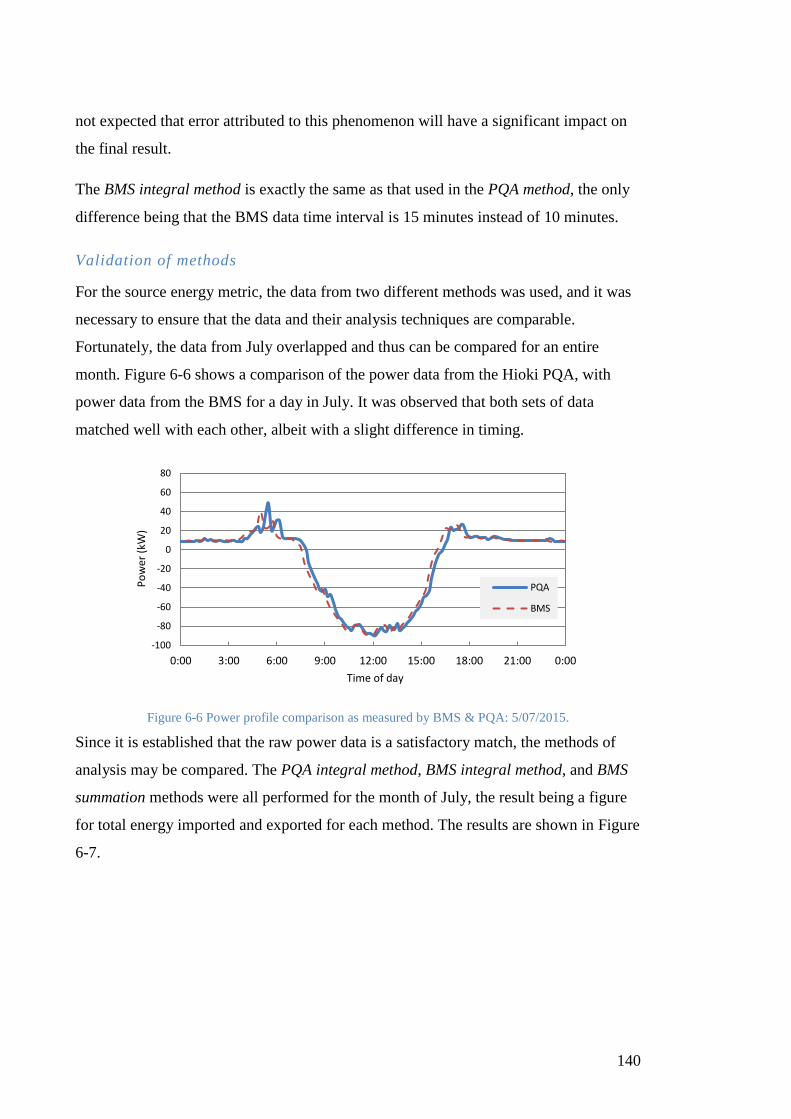
140
not expected that error attributed to this phenomenon will have a significant impact on
the final result.
The BMS integral method is exactly the same as that used in the PQA method, the only
difference being that the BMS data time interval is 15 minutes instead of 10 minutes.
Validation of methods
For the source energy metric, the data from two different methods was used, and it was
necessary to ensure that the data and their analysis techniques are comparable.
Fortunately, the data from July overlapped and thus can be compared for an entire
month. Figure 6-6 shows a comparison of the power data from the Hioki PQA, with
power data from the BMS for a day in July. It was observed that both sets of data
matched well with each other, albeit with a slight difference in timing.
Figure 6-6 Power profile comparison as measured by BMS & PQA: 5/07/2015.
Since it is established that the raw power data is a satisfactory match, the methods of
analysis may be compared. The PQA integral method, BMS integral method, and BMS
summation methods were all performed for the month of July, the result being a figure
for total energy imported and exported for each method. The results are shown in Figure
6-7.
-100
-80
-60
-40
-20
0
20
40
60
80
0:00 3:00 6:00 9:00 12:00 15:00 18:00 21:00 0:00
Po
wer
(kW
)
Time of day
PQA
BMS

141
Figure 6-7 Comparison of imported/exported calculation methodologies.
Numerical values are recorded in Table 6-1 along with their relative errors compared to
the PQA integral method. A maximum error of 1.5% is recorded for the month of July.
This indicates that the methods used to determine imported and exported energy from
the SBRC on a monthly basis are sufficiently accurate as to provide confidence in the
SBRC buildings net zero energy source metric results.
Table 6-1 Comparison of errors for imported/exported calculation methodologies.
Imported (kWh) Exported (kWh)
PQA Integral Method 8169.38 -10917.15
BMS Integral Method 8047.22 -10815.80
BMS Separated Summation 8269.80 -10765.20
PQA Integral Method - -
BMS Integral Method 1.50% 0.93%
BMS Separated Summation -1.23% 1.39%
Figure 6-8 shows the energy consumption, generation, and net balance for each month
of 2015 according to the source metric. These results confirm that the building makes an
even more valuable contribution to decarbonizing of the built environment than in the
site metric due to the surplus energy it produces which avoids consumption of fossil
fuel generated grid electricity.
-15000
-10000
-5000
0
5000
10000
Imported (kWh) Exported (kWh)
Ener
gy (
kWh
)
PQA Integral Method BMS Integral Method BMS Summation

142
Figure 6-8 SBRC monthly source energy balance: 2015.
The primary energy factor (PEF) of 3.07 as discussed in Section 6.1 is applied on both
sides of the energy equation. Whilst this increases the primary energy associated with
imported energy, it also increases the primary energy consumption that is avoided
thanks to the export of surplus energy. Exported energy from the SBRC building is used
by other buildings on the same campus and thus saved them importing energy from the
grid with the 3.07 primary energy factor.
The cumulative source energy balance for 2015 is shown below in Figure 6-9.
Figure 6-9 SBRC cumulative source energy balance: 2015.
The total energy imported from the grid for the year was 197,708 kWh, an average of
541 kWh per day. Total energy exported to the grid was 526,517 kWh, averaging
1,443 kWh per day. The surplus of primary energy at the end of 2015 was 330 MWh.
A comparison of the cumulative net energy balance throughout the year for the site and
source metrics is shown in Figure 6-10. When the source metric is considered, the
-80000
-60000
-40000
-20000
0
20000
40000
Jan Feb Mar Apr May Jun Jul Aug Sep Oct Nov Dec
Ener
gy (
kWh
/mo
nth
)
Exported x PEF Imported x PEF Net Source Energy
-600000
-500000
-400000
-300000
-200000
-100000
0
100000
200000
300000
Jan Feb Mar Apr May Jun Jul Aug Sep Oct Nov Dec
Ener
gy (
kWh
)
Cumulative Import Cumulative Export Cumulative net
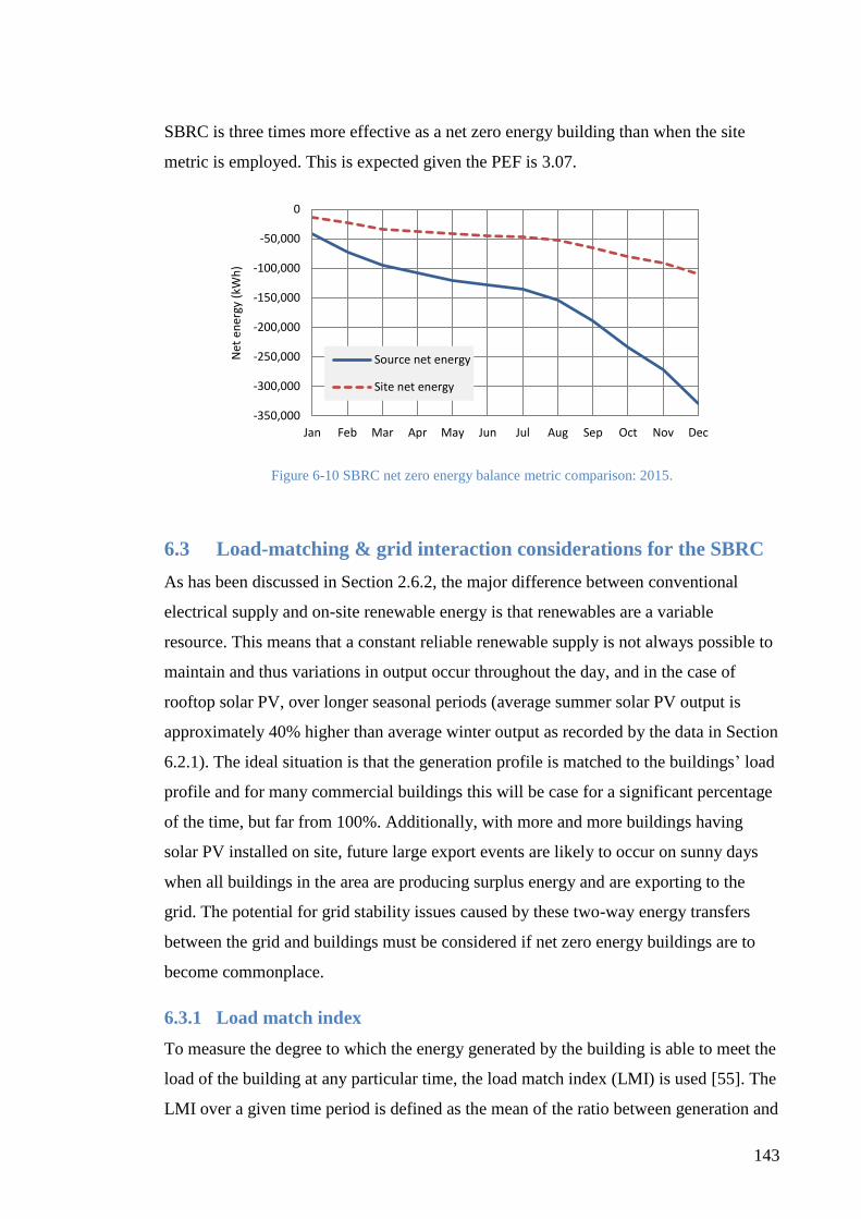
143
SBRC is three times more effective as a net zero energy building than when the site
metric is employed. This is expected given the PEF is 3.07.
Figure 6-10 SBRC net zero energy balance metric comparison: 2015.
6.3 Load-matching & grid interaction considerations for the SBRC
As has been discussed in Section 2.6.2, the major difference between conventional
electrical supply and on-site renewable energy is that renewables are a variable
resource. This means that a constant reliable renewable supply is not always possible to
maintain and thus variations in output occur throughout the day, and in the case of
rooftop solar PV, over longer seasonal periods (average summer solar PV output is
approximately 40% higher than average winter output as recorded by the data in Section
6.2.1). The ideal situation is that the generation profile is matched to the buildings’ load
profile and for many commercial buildings this will be case for a significant percentage
of the time, but far from 100%. Additionally, with more and more buildings having
solar PV installed on site, future large export events are likely to occur on sunny days
when all buildings in the area are producing surplus energy and are exporting to the
grid. The potential for grid stability issues caused by these two-way energy transfers
between the grid and buildings must be considered if net zero energy buildings are to
become commonplace.
6.3.1 Load match index
To measure the degree to which the energy generated by the building is able to meet the
load of the building at any particular time, the load match index (LMI) is used [55]. The
LMI over a given time period is defined as the mean of the ratio between generation and
-350,000
-300,000
-250,000
-200,000
-150,000
-100,000
-50,000
0
Jan Feb Mar Apr May Jun Jul Aug Sep Oct Nov Dec
Net
en
ergy
(kW
h)
Source net energy
Site net energy

144
load for each time step. Where the generation exceeds the load, the LMI for that time
step is equal to one. The LMI will never be more than one. This is because it is simply a
measure of how well the present load is met by on-site renewable generation at that
time. If the generation output is more than or equal to the load, the load is being met
100% by generation, regardless of how much it exceeds the magnitude of the load.
The LMI is affected by the time interval of data used. For a net zero or net positive
building, the LMI will be equal to one when viewing its annual energy balance.
However, on shorter timescales, the generation will not always match the load. On a
daily basis, with only solar PV and without storage, the generation will not match load
as generation is not possible outside of sunlight hours. This means that the LMI will be
less than one. To ensure a more accurate LMI, high resolution data should be used [54].
For this study, the data time interval used was 15 minutes. Ideally a full year of 15-
minute data would be available however, in this case, only data from July to the end of
2015 was available. This will still give a good indication of the overall average LMI for
the year as summer and winter seasons are still well represented in the data. An average
representative day of generation and load at the SBRC building is shown below in
Figure 6-11. One aspect to note is the early morning peak in the consumption profile.
This is caused by early morning pre-heating and cooling of the concrete hydronic slab
system, particularly in winter.
Figure 6-11 SBRC average load and generation profiles: 2015.
Visual inspection of the chart indicates that the load is matched (remembering the
surplus is ignored when considering the LMI) roughly 40 to 50% of the entire day. The
relatively flat load profile of the building makes the visual estimate of the LMI simple.
-20
0
20
40
60
80
100
0:00 3:00 6:00 9:00 12:00 15:00 18:00 21:00 0:00
Po
wer
(kW
)
Time of day
Average Gen (kW)
Average Load (kW)

145
Using the 15-minute data from July to the end of December the LMI is described as
follows:
The ratio between generation and load is calculated for each data point:
𝐿𝑀𝐼𝑖 = min (1,
𝑃𝑔𝑒𝑛,𝑖
𝑃𝑙𝑜𝑎𝑑,𝑖) (6.2)
Where i is the value at each time step, Pgen is the generation power output for a
given time and Pload is the load at the given time. This is the simplest form of the
LMI equation, where storage and any system losses are ignored.
This is calculated for every n time-step in the data set. The mean of the LMI for
all data points is then calculated to give the LMI for the time period considered:
𝐿𝑀𝐼 = ∑𝐿𝑀𝐼
𝑛
𝑖=1
(6.3)
For the SBRC building, using the data available, the average LMI for the six-month
period July to December was calculated to be 43.5%. The average LMI for the average
24-hour period shown in Figure 6-11 (averaged from the same July to December data)
is 47.9%. This agrees well with the visual estimate made above.
The result means that the SBRC building, despite being a net positive building
throughout the year on a yearly, monthly, and frequently daily basis, is only able to
meet its own energy requirements 44% of the time when sub-hourly data is considered
due to overnight loads being unable to be matched with solar PV output which of course
cannot generate at night.
General suggestions for improving the LMI are to implement demand-side management
(DSM) strategies, as well as increase generation capacity. In the specific case of the
SBRC building, increasing generating capacity will not improve the situation, given that
the problem lies not in the output potential, but in the output timing. DSM, too, is
unlikely to have a significant effect on the LMI, given that the load profile of the
building is typically quite flat across the day.
One strategy which may improve the LMI is not to increase solar PV generating
potential, but to diversify the generation techniques. Installation of small-scale wind
turbines on the site could generate energy during the night where solar PV cannot.
However, this improvement would be intermittent, depending on the quality of the

146
variable wind resource at the site. The most promising method of improving the LMI at
the SBRC is to install battery storage. A large surplus is generated every day by the
solar PV system, excluding days of inclement weather. A battery storage system sized
to match the average or peak magnitude of overnight energy requirements would be
charged during the day at times of surplus generation and would discharge overnight
when the load exceeds generation.
6.3.2 Grid interaction index
Whilst the load match index measures the degree to which the generation of the
building is able to meet its load requirements, the grid interaction index (GII) measures
the variability of energy exchange with the grid over a particular time period. It is a
comparison of the net grid energy reading to the maximum value of net energy in the
time period. The GII explains the variability of energy exchanged with the grid by
taking the standard deviation of the GII for each time step of the time period. It is not
related to the magnitude of electricity required from the grid. The GII is calculated as
follows:
The net power reading of the main incomer at each time step is compared to the
maximum of the absolute value of net power in the dataset:
𝐺𝐼𝐼𝑖 =
𝑃𝑛𝑒𝑡,𝑖
𝑚𝑎𝑥|𝑃𝑛𝑒𝑡,𝑛| (6.4)
Where i is the value at each time step, and Pnet is the power reading at the main
incomer of the building.
GIIi is calculated for every n time step in the data set. The standard deviation of
the GIIi dataset is then calculated to give the average grid stress for the time
period considered:
𝐺𝐼𝐼𝑛 = 𝑆𝑇𝐷(𝐺𝐼𝐼𝑖) (6.5)
For the case study SBRC building, the GII for the year was calculated to be 0.22. Whilst
there is not yet a large volume of NZEBs reporting their GII’s in the literature, this
result is a good comparison with the small number of results reported for GII in [54].

147
6.3.3 Power quality considerations of net zero energy buildings
Net zero energy buildings typically utilise a range of high efficiency appliances, such as
lighting equipment. The impact of such equipment from the perspective of power
quality and the consequences for the grid needs to be considered. Whilst a detailed
analysis of these factors in relation to NZEBs is beyond the scope of this thesis, some
preliminary presentation of basic power quality data is provided here.
Power Factor
The first consideration for power quality in commercial buildings is often power factor.
Power factor is the ratio of real power (kW) to apparent power (kVA). While optimising
power factor, i.e. making it closer to unity, will have little effect on the energy use
internally within a net zero energy building, utilities provide incentive to increase power
factor through penalties for exceeding minimum power factors and indirectly via
demand charges (which are a function of apparent power). Accordingly, commercial
buildings will generally have a power factor correction unit, typically a large switched
capacitor bank, installed to increase power factor during high reactive power (kVAr)
demand periods.
Figure 6-12 SBRC 15-minute average power factor, real, and apparent power.
From Figure 6-12 it can be seen that the nominal power factor of the SBRC is close to
unity during both generation and non-generation periods. Note that M1 refers to the
meter number installed on the main incomer of the SBRC building. This is proposed to
be largely due to the combined power factor of high efficiency equipment such as LED
lighting, inverter based variable speed drives, etc., which will be synonymous with net
-1.5
-1
-0.5
0
0.5
1
1.5
-150
-100
-50
0
50
100
150
0:00 3:00 6:00 9:00 12:00 15:00 18:00 21:00 0:00
Po
wer
Fac
tor
Po
wer
(kW
, kV
A)
Time of day
M1 Power M1 Apparent Power M1 Calculated PF

148
zero energy buildings or buildings retrofitted for energy efficiency improvements. The
power factor of such equipment at the SBRC has negated the need for costly power
factor correction equipment to be installed. It is noted that in Australia, at present,
generation from the solar photovoltaic system inverters are required to deliver power to
the local load and grid at near unity power factor.
Harmonics
The operation of modern, high efficiency lighting technology produces significant
harmonic distortion in the currents that they draw from the power system. While
harmonic distortion levels are often factored into equipment standards to reduce their
impact on the grid, the high penetration of such devices in the low voltage distribution
system of net zero energy buildings needs to be understood. While power quality
analysis is beyond the primary scope of this thesis, some preliminary reporting on the
harmonic distortion levels, available from the installed sub metering equipment, is
presented here as a prelude to possible future research. Figure 6-13 shows that there is a
high level of harmonic distortion in the current drawn from the grid by the SBRC.
Figure 6-13 SBRC THD of voltage and current on a typical day.
The resulting harmonic distortion in the voltage is within acceptable limits [87]
however consideration of harmonics needs to be factored into the design of the
electrical system (rating of cables, etc.). It is also noted that operation of the solar
photovoltaic system inverters, i.e. in times of generation, reduces the levels of current
and voltage harmonic distortion on the system.
0
1
1
2
2
3
3
4
0
10
20
30
40
50
60
70
0:00 3:00 6:00 9:00 12:00 15:00 18:00 21:00 0:00 Vo
ltag
e To
tal H
arm
on
ic D
isto
rtio
n (
%)
Cu
rren
t To
tal H
arm
on
ic D
isto
rtio
n (
%)
Time of Day
SBRC Meter M1|Current THD SBRC Meter M1|Voltage THD
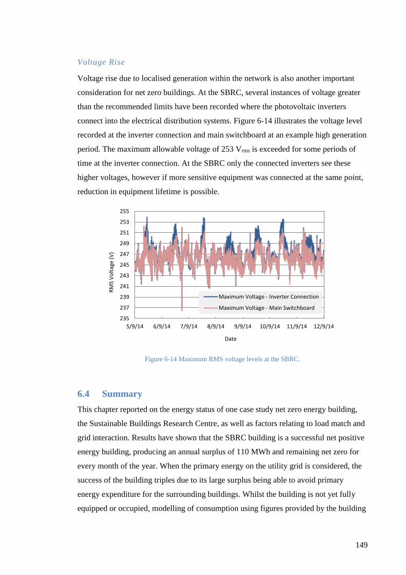
149
Voltage Rise
Voltage rise due to localised generation within the network is also another important
consideration for net zero buildings. At the SBRC, several instances of voltage greater
than the recommended limits have been recorded where the photovoltaic inverters
connect into the electrical distribution systems. Figure 6-14 illustrates the voltage level
recorded at the inverter connection and main switchboard at an example high generation
period. The maximum allowable voltage of 253 Vrms is exceeded for some periods of
time at the inverter connection. At the SBRC only the connected inverters see these
higher voltages, however if more sensitive equipment was connected at the same point,
reduction in equipment lifetime is possible.
Figure 6-14 Maximum RMS voltage levels at the SBRC.
6.4 Summary
This chapter reported on the energy status of one case study net zero energy building,
the Sustainable Buildings Research Centre, as well as factors relating to load match and
grid interaction. Results have shown that the SBRC building is a successful net positive
energy building, producing an annual surplus of 110 MWh and remaining net zero for
every month of the year. When the primary energy on the utility grid is considered, the
success of the building triples due to its large surplus being able to avoid primary
energy expenditure for the surrounding buildings. Whilst the building is not yet fully
equipped or occupied, modelling of consumption using figures provided by the building
235
237
239
241
243
245
247
249
251
253
255
5/9/14 6/9/14 7/9/14 8/9/14 9/9/14 10/9/14 11/9/14 12/9/14
RM
S V
olt
age
(V)
Date
Maximum Voltage - Inverter Connection
Maximum Voltage - Main Switchboard

150
design consultants indicate that the building will still easily achieve net zero when fully
occupied.
An analysis of how the SBRC building is able to match its generation and load profiles,
and how it interacts with the grid was also performed. The reported Load Match Index
was found to be 43.5% for the second half of 2015. The GII for 2015 was found to be
0.22. It is desirable for the GII to be as low as possible. Electrical equipment must be
designed for peak loading. Significant infrastructure savings can be found in reducing
the expected peak loads in a system. The LMI, together with the GII provide a means to
quantify how the building interacts with the utility grid. Peak import and export events
can be reduced through implementation of load matching improvement measures to
minimise interaction of the building with the grid. A high GII means the building has a
highly variable relationship with the grid, ranging from high levels of import or export
to having little interaction at all. Since infrastructure is designed for extreme cases
which may happen only on very rare occasions, reduction of grid interaction variability
can save significant costs by lowering the levels with which infrastructure must cope.
While energy generation and use is of primary importance to NZEB design, other
considerations associated with the energy delivery system need to be included during
design, e.g. power factor and power quality requirements. While such considerations are
relevant to all buildings, the uniqueness of NZEBs means that power factor correction
equipment may be omitted in some cases, and the electrical distribution system needs to
be able to mitigate the harmonics of high energy efficiency equipment as well as voltage
rise from localised generation.

151
Chapter 7 Conclusion and Future Work
As a promising design philosophy in the future of the built environment, the success of
net zero energy buildings depends greatly on a good understanding of the influence that
different design factors have on the energy performance of a building. The importance
of design and operational factors to the success of net zero energy buildings has been
investigated through the use of building performance simulation. This research entailed
the development of building performance models for three case study buildings as well
as a comprehensive validation methodology for each model.
7.1 Building model validation
This thesis demonstrated that validation of models of efficient buildings is more
challenging than models of conventional buildings due to intelligent systems which are
able to adjust their behaviour automatically depending on a range of environmental
variables such as available natural light. This has the effect of making energy
consumption of these systems more variable than in a conventional building and thus
more difficult to model where provision of specific environmental inputs is not made.
Natural ventilation in building models is not as easily predicted as behaviour of artificial
HVAC systems. More complex modelling techniques which consider the intricacies of
internal and external airflow interactions with the building envelope would possibly
provide more accurate results.
A methodology to successfully validate building models and simulation results was
developed. Successful validation of building models is dictated heavily by the
availability and reliability of measured building data. Both energy consumption for the
main building systems (HVAC, lighting, building services), as well as temperature data
for summer and winter periods for several zones within the building, are recommended
to ensure the building not only exhibits characteristic energy consumption behaviour,
but that the building responds properly in a thermal respect. One challenge encountered
in this study was obtaining adequate data for all test cases. No thermal data was
available for the Enterprise 1 building, while very little energy data was obtainable from
the TTT building. Had a longer timeframe been available for data acquisition, a better
result may have been achieved regarding the validation of the case study building

152
models. Nonetheless, the modelling performed here can be regarded as adequate, given
that results are compared to a benchmark of the same building model for each scenario.
7.2 Building simulation results
Simulations were undertaken to investigate the performance of net zero energy
buildings. The effectiveness of various designs and operating parameters were modelled
to gain an understanding of the most effective way of reducing energy consumption and
achieving net zero energy in a building. The net zero energy case study buildings
studied here indicated from simulation results that efficient buildings are more sensitive
to changes in design or operating practices than more conventional buildings. This
suggests that a building designed from scratch for the purpose of being net zero will
have the best chance of achieving that goal. A retrofitted building may not achieve this
goal as easily due to factors such as the building envelope not being designed to be able
to capture the maximum amount of daylight to aid in reducing lighting loads. Another
factor which may affect the outcome of a retrofitted building compared to a NZEB
designed from scratch is that the building layout may not lend itself to successful
natural ventilation implementation. Ideally a building with a successful natural
ventilation scheme will be designed with cross-flow of air in mind: open plan spaces
with large atrium common areas enabling airflow between different levels of the
building. Buildings should be narrow to maintain sufficient air distribution throughout
the interior.
The research undertaken in this thesis indicated that significant benefits to energy
consumption are possible with the installation of high performance glazing. Energy
savings between 6% and 11% are possible in net zero buildings when triple glazed, low
emissivity glass is used compared to a benchmark of single glazed, clear glass. Higher
performance glazing presented less of a benefit for the conventional building due to
HVAC loads (the aspect most effected by glazing) being less dominant than in the
NZEBs.
Simulations of building models and complimentary data collection from case study
buildings have shown that controlling lighting output in proportion to the available
amount of daylight present in a room also presents significant benefits to energy
reduction in buildings. Large open plan spaces with high levels of external and internal

153
glazing benefit most from this, enabling maximum transmission and penetration of
natural light into the building. This is where design intent is important and where older,
more conventional buildings may not achieve benefits. Enterprise 1, the conventional
building studied here, was designed with open plan offices, as well as large atriums with
skylights at each end of the building. This makes it a very good candidate for the
retrofitting of daylighting controls. Simulation results suggested an overall saving of
25% to total building energy use. This is a significant saving due as lighting is one of
the most dominant loads in this building. In the TTT building, an overall saving of 21%
was determined compared to a scenario where daylight controls were not installed,
while at the SBRC, it was found that due to the already very low lighting power density
specified in the design phase, daylight controls contribute to only an 8% energy saving.
The implications for energy consumption from window shading controlled by both time
of day and outdoor temperature were investigated. Overall, the net benefit to total
energy consumption in each building was insignificant, if there was a benefit at all.
Typically, any improvement due to reduction in HVAC loads was cancelled out by the
need for significant increases in lighting use to compensate for lost daylight.
From simulations performed on the case study building models, adjustments of HVAC
setpoint offer meaningful energy savings. Net zero buildings appear most sensitive to
changes in HVAC setpoints but it must be considered that the default setpoints are
wider than usual to begin with. It is important that any changes to HVAC setpoints must
meet the perceived comfort standard of occupants to ensure a comfortable environment
indoors. Increasing the cooling setpoint from 24°C to 26°C at the Enterprise 1 building
was predicted to result in a 25% energy saving, however this would not be feasible if
occupants were not comfortable while in the building.
7.3 Energy balance & grid considerations of case study NZEB
Analysis of a full year of data available for the Sustainable Buildings Research Centre
building has enabled the net zero status of the building for 2015 to be established. The
position of the SBRC was successful, generating an annual energy surplus of 110 MWh
and maintaining a surplus throughout every month of 2015 based on the site energy
metric (a comparison of energy consumed to energy generated). The analysis included
consideration of the primary energy factor of the utility grid, calculated in order to

154
assess the source energy balance (a comparison of energy imported to energy exported).
With a primary energy factor of 3.07 established based on the most recent data
available, the source energy balance for the SBRC improved the contribution of the
building to emissions reduction by a factor of three. The large surplus of energy
produced is used elsewhere on the campus, thereby avoiding the expense of primary
energy associated with imports from the utility grid.
Analysis of the load match and grid interaction factors at the SBRC provided an
indication of what possible challenges high numbers of NZEBs will present to the utility
grid in the future. Maximising the ability for the building to cover all of its own loads
with on-site generation at all times of the day, as well as minimising the variance of
energy transfer between the grid and building is important to reduce grid infrastructure
capital and maintenance costs. The Load Match index for the SBRC based on available
data of 15-minute intervals was calculated to be 43.5%. The Grid Interaction Index was
calculated to be 0.22. With the increasing affordability of battery storage, this
technology makes the prospects of improving the Load Match Index much easier.
Surplus energy generated during the day is stored for overnight use. Additionally,
diversification of on-site renewable technology through the addition of small-scale wind
turbines would also serve to improve the Load Match Index.
The balance of energy generated and consumed is of primary importance to the field of
net zero energy buildings; however, considerations must be made regarding power
quality. Primarily the power factor, total harmonic distortion, and voltage rise must be
considered in the design phase of buildings. The general overview and brief analysis of
these factors for the SBRC case study suggest that power factor correction equipment
may not be necessary in some cases.
7.4 Suggested future research
Upon the fulfilment of the aim and objectives of this thesis, several areas of potential
research have been identified:
• Further efforts to more comprehensively validate each building model using a
complete year of temperature and energy data. This would improve the

155
confidence of the results of this thesis, and also enable further study in other
areas of building research using robust and reliable building model case studies.
• Whilst the effects of window shading on energy consumption for the three test
cases were simulated, the subject of shading elements in buildings is a broad one
and should consider many interrelated variables. This made the study of this
field, using differing case study buildings, difficult given that each building has
its own location and building-specific shading elements already built-in. Further
understanding of the effects of building shading elements on energy
consumption would be gained through a separate study using a hypothetical
model on which to investigate such factors as roof and window overhangs,
vertical wall and window fins, and the placement of surrounding features such as
buildings and vegetation. The ‘all-or-nothing’ approach to window shading
modelling performed in this study led to poor results. However, investigation of
more nuanced and subtle shading devices may find a positive and significant
effect on energy consumption.
• Important questions regarding occupant interaction with buildings and their
effects on energy consumption were raised in this thesis. However, the
modelling methodology employed did not lend itself to the study of occupant
behaviour. One potential area of research in this field would be how energy
consumption and efficiency initiatives shape the behaviour of occupants in a
building and whether these initiatives conflict with occupant needs and
preferences. It is suggested that net zero energy buildings will be more
successful if their occupants embody a culture of energy conservation, however
this would warrant further investigation. A successful NZEB would be one
which requires little habitual and cultural change from its occupants as this may
present a barrier to widespread up-take.
• This study focussed on the modelling of three case study buildings conveniently
situated in close proximity to each other. This made validation of each model
simpler and the results were able to be compared on a level basis. However, the
three buildings had differing sizes and purposes. These two factors are likely to
affect energy consumption and thus some conclusions made here may not be
able to be applied more broadly to buildings in general with total confidence.

156
More work should be undertaken with a higher sample size of case study
buildings, both NZEB and conventional, in order to build up a reliable picture of
factors which drive energy savings in NZEBs and how they compare to
conventional buildings.
• A brief overview of the power quality factors which warrant consideration in the
design of a NZEB was given in this thesis. This is a field where deeper research
is necessary to understand how large numbers of net zero buildings interact fully
with the grid and what implications this may have in the field of power quality.
157
Appendices
Appendix A. R2 plots omitted from Section 4.4.2
Figure A-1 R2 for SBRC energy lab room temperature comparison - winter
Figure A-2 R2 for SBRC Eastern Office temperature comparison - summer
R² = 0.0002
15
17
19
21
23
15 16 17 18 19 20 21 22 23
Mo
del
(°C
)
Measured (°C)
Power lab - Model vs Measured
R² = 0.01
19
21
23
25
27
19 20 21 22 23 24 25 26 27
Mo
del
(°C
)
Measured (°C)
Eastern Office - Model vs Measured
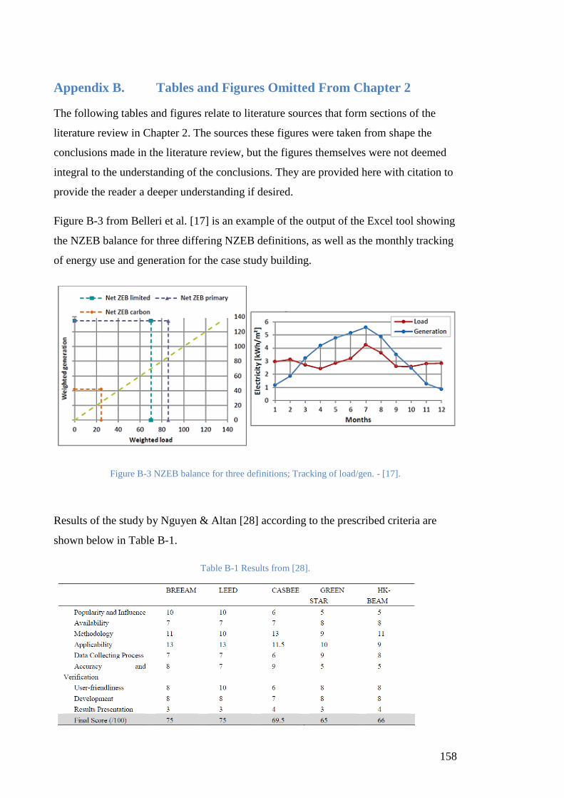
158
Appendix B. Tables and Figures Omitted From Chapter 2
The following tables and figures relate to literature sources that form sections of the
literature review in Chapter 2. The sources these figures were taken from shape the
conclusions made in the literature review, but the figures themselves were not deemed
integral to the understanding of the conclusions. They are provided here with citation to
provide the reader a deeper understanding if desired.
Figure B-3 from Belleri et al. [17] is an example of the output of the Excel tool showing
the NZEB balance for three differing NZEB definitions, as well as the monthly tracking
of energy use and generation for the case study building.
Figure B-3 NZEB balance for three definitions; Tracking of load/gen. - [17].
Results of the study by Nguyen & Altan [28] according to the prescribed criteria are
shown below in Table B-1.
Table B-1 Results from [28].

159
Table B-2 is an excerpt from Dubois & Blomsterberg [38] showing the type of energy
saving strategy and it’s potential for savings.
Table B-2 Energy savings potential of different strategies by [38].

160
Appendix C. Data Sets
All data sets relating to building models, measured building data, simulation results, and
weather files are stored in the Sustainable Buildings Research Centre data repository
and are available upon request to the author or to the SBRC directly. A list of available
files is given below:
Table C-3 List of available data related to this thesis
File No. File Name File Type Relating to:
1 SBRC Monthly Energy Balance .xlsx SBRC
2 Model EUB’s .xlsx ALL
3 SBRC – DRAFT Building Users Guide .pdf SBRC
4 1004305 Uni of Wollongong_SBRC_TEC Report – Rev C .pdf SBRC
5 SBRC MECH Drawings .pdf SBRC
6 SBRC ELEC Drawings .pdf SBRC
7 WSP Mechanical Services Specification .pdf SBRC
8 TTT ARCH Drawings .pdf TTT
9 TTT MECH Drawings .pdf TTT
10 TTT ELEC Drawings .pdf TTT
11 AC 1 Energy report Jan to April 15 .pdf TTT
12 AC 2 Energy report Jan to April 15 .pdf TTT
13 AC 3 Energy report Jan to April 15 .pdf TTT
14 Level 1 lighting year to date .xlsx TTT
15 Level 1 power year to date .xlsx TTT
16 Level O lighting year to date .xlsx TTT
17 RRSB year to date .xlsx TTT
18 TTT Energy Data .xlsx TTT
19 Yea to date level O power .xlsx TTT
20 Water Furnace Specs .pdf TTT
21 Enterprise 1 ARCH Drawings .pdf E1
22 Asset List & Synthetic Breakdown .pdf E1
23 Enterprise-1 Manual .pdf E1
24 iCE1 Volume 1 Building Works .pdf E1
25 Lighting Sheets .pdf E1

161
26 DesignBuilder TTT .zip TTT
27 DesignBuilder SBRC .zip SBRC
28 DesignBuilder Enterprise One .zip E1
29 BMS Data .zip SBRC
30 Aust electrical breakdown .xlsx ALL
31 Bellambi TMY DB temp histogram .xlsx ALL
32 SBRC Incomer HIOKI Power Data 2015 02-01-15 to 31-07-16 –chapter 6 .xlsx SBRC
33 Glazing Simulations .xlsx ALL
34 Glazing simulations_Identical lighting system .xlsx ALL
35 Glazing simulations_Identical lighting system_no control .xlsx ALL
36 HVAC SP analysis .xlsx ALL
37 Lighting Control simulations .xlsx ALL
38 Shading analysis .xlsx ALL
162
References
[1] L. Guan, “Energy use, indoor temperature and possible adaptation strategies for
air-conditioned office buildings in face of global warming,” Building and
Environment, vol. 55, pp. 8–19, Sep. 2012.
[2] X. Wang, D. Chen, and Z. Ren, “Assessment of climate change impact on
residential building heating and cooling energy requirement in Australia,”
Building and Environment, vol. 45, no. 7, pp. 1663–1682, Jul. 2010.
[3] International Living Future Institute, “Living Building Challenge,” 2015.
[Online]. Available: http://living-future.org/lbc. [Accessed: 04-Apr-2016].
[4] D. H. W. Li, L. Yang, and J. C. Lam, “Zero energy buildings and sustainable
development implications – A review,” Energy, vol. 54, pp. 1–10, Jun. 2013.
[5] L. Pérez-Lombard, J. Ortiz, and C. Pout, “A review on buildings energy
consumption information,” Energy and Buildings, vol. 40, no. 3, pp. 394–398,
Jan. 2008.
[6] International Energy Agency, “World Energy Outlook,” Paris, 2013.
[7] P. de Wilde and D. Coley, “The implications of a changing climate for
buildings,” Building and Environment, vol. 55, pp. 1–7, Sep. 2012.
[8] Z. Ren, Z. Chen, and X. Wang, “Climate change adaptation pathways for
Australian residential buildings,” Building and Environment, vol. 46, no. 11, pp.
2398–2412, Nov. 2011.
[9] P. Wilkinson, K. R. Smith, M. Davies, H. Adair, B. G. Armstrong, M. Barrett, N.
Bruce, A. Haines, I. Hamilton, T. Oreszczyn, I. Ridley, C. Tonne, and Z. Chalabi,
“Public health benefits of strategies to reduce greenhouse-gas emissions:
household energy.,” Lancet, vol. 374, no. 9705, pp. 1917–29, Dec. 2009.
[10] J. A. Clarke, C. M. Johnstone, N. J. Kelly, P. A. Strachan, and P. Tuohy, “The
role of built environment energy efficiency in a sustainable UK energy
economy,” Energy Policy, vol. 36, no. 12, pp. 4605–4609, Dec. 2008.
[11] P. Torcellini, S. Pless, M. Deru, and D. Crawley, “Zero energy buildings: a
critical look at the definition,” in NREL/CP-550-39833, 2006.
[12] I. Sartori, A. Napolitano, and K. Voss, “Net zero energy buildings: A consistent

163
definition framework,” Energy and Buildings, vol. 48, pp. 220–232, May 2012.
[13] I. Sartori, A. Napolitano, A. J. Marszal, S. Pless, P. Torcellini, and K. Voss,
“Criteria for definition of net zero energy buildings,” in International Conference
on Solar Heating, Cooling and Buildings (EuroSun 2010), 2010.
[14] A. J. Marszal, P. Heiselberg, J. S. Bourrelle, E. Musall, K. Voss, I. Sartori, and
A. Napolitano, “Zero Energy Building – A review of definitions and calculation
methodologies,” Energy and Buildings, vol. 43, no. 4, pp. 971–979, Apr. 2011.
[15] S. Pless and P. Torcellini, “Net-Zero Energy Buildings : A Classification System
Based on Renewable Energy Supply Options,” National Renewable Energy
Laboratory, 2010.
[16] B. Griffith, N. Long, P. Torcellini, R. Judkoff, D. Crawley, and J. Ryan,
“Assessment of the Technical Potential for Achieving Net Zero-Energy Buildings
in the Commercial Sector Assessment of the Technical Potential for Achieving
Net Zero-Energy Buildings in the Commercial Sector,” National Renewable
Energy Laboratory, 2007.
[17] A. Belleri, F. Noris, U. . Oberegger, and R. Lollini, “Evaluation Tool For Net
Zero Energy Buildings: Application On Office Building,” in Proceedings of the
World Sustainable Energy Days, Wels, Austria 27, 2013.
[18] F. Noris, A. Napolitano, and R. Lollini, “Measurement and Verification protocol
for Net Zero Energy Buildings,” IEA SHC/ECBCS Task 40/Annex 52 – Towards
Net Zero Energy solar Buildings, 2013.
[19] A. . Marszal, J. . Bourrelle, E. Musall, P. Heiselberg, A. Gustavsen, and K. Voss,
“Net Zero Energy Buildings-Calculation Methodologies versus National Building
Codes,” in Proceedings of EuroSun (2010), 2010, vol. 2, no. May 2010.
[20] H. Rasekh, “Delivering the vision of sustainable buildings,” University of
Wollongong, 2013.
[21] Building Research Establishment Ltd, “Why BREEAM?,” 2015. [Online].
Available: http://www.breeam.org/about.jsp?id=66. [Accessed: 04-Apr-2016].
[22] BRE Global Limited, “BREEAM: International,” 2012. [Online]. Available:
http://www.breeam.org/podpage.jsp?id=367. [Accessed: 29-Aug-2014].
[23] U.S. Green Building Council, “LEED Rating Systems,” 2016. [Online].

164
Available: http://www.usgbc.org/leed#rating. [Accessed: 04-Apr-2016].
[24] New South Wales Office of Environment and Heritage, “How NABERS Works,”
2014. [Online]. Available:
http://www.nabers.gov.au/public/WebPages/ContentStandard.aspx?module=10&
template=3&id=5&include=HowNabersWorks.htm&side=factsheets.htm.
[Accessed: 01-Sep-2014].
[25] Green Building Council of Australia, “Introducing Green Star,” 2013.
[26] Green Building Council of Australia, “The Value of Green Star - A Decade of
Environmental Benefits,” 2013.
[27] Y. Roderick, D. McEwan, C. Wheatley, and C. Alonso, “Comparison of energy
performance assessment between LEED, BREEAM and Green Star,” in Eleventh
International IBPSA Conference, Glasgow, Scotland, 27-30 July 2009, 2009, pp.
1167–1176.
[28] B. K. Nguyen and H. Altan, “Comparative Review of Five Sustainable Rating
Systems,” in 2011 International Conference on Green Buildings and Sustainable
Cities, 2011, vol. 21, pp. 376–386.
[29] S. M. Bambrook, A. B. Sproul, and D. Jacob, “Design optimisation for a low
energy home in Sydney,” Energy and Buildings, vol. 43, no. 7, pp. 1702–1711,
Jul. 2011.
[30] G. K. Oral, A. K. Yener, and N. T. Bayazit, “Building envelope design with the
objective to ensure thermal, visual and acoustic comfort conditions,” Building
and Environment, vol. 39, no. 3, pp. 281–287, Mar. 2004.
[31] A. Syed, Advanced building technologies for sustainability, vol. 3. John Wiley &
Sons, 2012.
[32] H. Sozer, “Improving energy efficiency through the design of the building
envelope,” Building and Environment, vol. 45, no. 12, pp. 2581–2593, Dec.
2010.
[33] R. Pacheco, J. Ordóñez, and G. Martínez, “Energy efficient design of building: A
review,” Renewable and Sustainable Energy Reviews, vol. 16, no. 6, pp. 3559–
3573, Aug. 2012.
[34] S. B. Sadineni, S. Madala, and R. F. Boehm, “Passive building energy savings: A

165
review of building envelope components,” Renewable and Sustainable Energy
Reviews, vol. 15, no. 8, pp. 3617–3631, Oct. 2011.
[35] C. Franzetti, G. Fraisse, and G. Achard, “Influence of the coupling between
daylight and artificial lighting on thermal loads in office buildings,” Energy and
Buildings, vol. 36, no. 2, pp. 117–126, Feb. 2004.
[36] M. Bodart and A. De Herde, “Global energy savings in offices buildings by the
use of daylighting,” Energy and Buildings, vol. 34, no. 5, pp. 421–429, Jun.
2002.
[37] M. Krarti, P. M. Erickson, and T. C. Hillman, “A simplified method to estimate
energy savings of artificial lighting use from daylighting,” Building and
Environment, vol. 40, no. 6, pp. 747–754, Jun. 2005.
[38] M.-C. Dubois and Å. Blomsterberg, “Energy saving potential and strategies for
electric lighting in future North European, low energy office buildings: A
literature review,” Energy and Buildings, vol. 43, no. 10, pp. 2572–2582, Oct.
2011.
[39] P. Hoes, J. L. M. Hensen, M. G. L. C. Loomans, B. de Vries, and D. Bourgeois,
“User behavior in whole building simulation,” Energy and Buildings, vol. 41, no.
3, pp. 295–302, Mar. 2009.
[40] Z. Yu, B. C. M. Fung, F. Haghighat, H. Yoshino, and E. Morofsky, “A
systematic procedure to study the influence of occupant behavior on building
energy consumption,” Energy and Buildings, vol. 43, no. 6, pp. 1409–1417, Jun.
2011.
[41] R. V. Andersen, J. Toftum, K. K. Andersen, and B. W. Olesen, “Survey of
occupant behaviour and control of indoor environment in Danish dwellings,”
Energy and Buildings, vol. 41, no. 1, pp. 11–16, Jan. 2009.
[42] O. T. Masoso and L. J. Grobler, “The dark side of occupants’ behaviour on
building energy use,” Energy and Buildings, vol. 42, no. 2, pp. 173–177, Feb.
2010.
[43] L. Klein, J. Kwak, G. Kavulya, F. Jazizadeh, B. Becerik-Gerber, P. Varakantham,
and M. Tambe, “Coordinating occupant behavior for building energy and
comfort management using multi-agent systems,” Automation in Construction,

166
vol. 22, pp. 525–536, Mar. 2012.
[44] M. Boxwell, Solar Electricity Handbook: A Simple, Practical Guide to Solar
Energy: how to Design and Install Photovoltaic Solar Electric Systems.
Greenstream Publishing, 2012.
[45] P. Gevorkian, Solar power in building design: the engineer’s complete design
resource. McGraw-Hill, 2008.
[46] Volker Quaschning, “Technology Fundamentals: The Sun as an Energy
Resouce,” 2003. [Online]. Available: http://www.volker-
quaschning.de/articles/fundamentals1/index_e.php. [Accessed: 18-Sep-2014].
[47] G. Stapleton, S. Neill, and G. Milne, “Photovoltaic systems | YourHome,” 2013.
[Online]. Available: http://www.yourhome.gov.au/energy/photovoltaic-systems.
[Accessed: 18-Sep-2014].
[48] A. F. Sherwani and J. A. Usmani, “Life cycle assessment of solar PV based
electricity generation systems: A review,” Renewable and Sustainable Energy
Reviews, vol. 14, no. 1, pp. 540–544, Jan. 2010.
[49] D. Simms, “Wind energy update,” National Renewable Energy Laboratory, 2008.
[50] A. S. Bahaj, L. Myers, and P. A. B. James, “Urban energy generation: Influence
of micro-wind turbine output on electricity consumption in buildings,” Energy
and Buildings, vol. 39, no. 2, pp. 154–165, Feb. 2007.
[51] P. Cooper, X. Liu, P. Kosasih, and R. Yan, “Modelling net zero energy options
for a sustainable buildings research centre,” in 12th Conference of International
Building Performance Simulation Association, Building Simulation 2011
Conference, 2011, pp. 2799–2806.
[52] A. D. Peacock, D. Jenkins, M. Ahadzi, A. Berry, and S. Turan, “Micro wind
turbines in the UK domestic sector,” Energy and Buildings, vol. 40, no. 7, pp.
1324–1333, Jan. 2008.
[53] N. Mithraratne, “Roof-top wind turbines for microgeneration in urban houses in
New Zealand,” Energy and Buildings, vol. 41, no. 10, pp. 1013–1018, Oct. 2009.
[54] K. Voss, I. Sartori, A. Napolitano, S. Geier, H. Gonzalves, M. Hall, P.
Heiselberg, J. Widén, J. A. Candanedo, E. Musall, B. Karlsson, and P. Torcellini,
“Load matching and grid interaction of net zero energy buildings,” in EUROSUN

167
2010 International Conference on Solar Heating, Cooling and Buildings, 2010.
[55] J. Salom, A. J. Marszal, J. A. Candanedo, J. Widén, K. B. Lindberg, and I.
Sartori, “Analysis of load match and grid interaction indicators in net zero energy
buildings with high-resolution data,” 2014.
[56] J. Salom, J. Widén, and J. Candanedo, “Understanding net zero energy buildings:
evaluation of load matching and grid interaction indicators,” in 12th Conference
of International Building Performance Simulation Association, Sydney, 14-16
November, 2011, vol. 6, pp. 14–16.
[57] S. Deng, R. Z. Wang, and Y. J. Dai, “How to evaluate performance of net zero
energy building – A literature research,” Energy, vol. 71, pp. 1–16, Jun. 2014.
[58] A. J. Marszal, P. Heiselberg, R. Lund Jensen, and J. Nørgaard, “On-site or off-
site renewable energy supply options? Life cycle cost analysis of a Net Zero
Energy Building in Denmark,” Renewable Energy, vol. 44, pp. 154–165, Aug.
2012.
[59] T. Ackermann, G. Andersson, and L. Söder, “Distributed generation: a
definition,” Electric Power Systems Research, vol. 57, no. 3, pp. 195–204, Apr.
2001.
[60] P. Järventausta, S. Repo, A. Rautiainen, and J. Partanen, “Smart grid power
system control in distributed generation environment,” Annual Reviews in
Control, vol. 34, no. 2, pp. 277–286, Dec. 2010.
[61] R. H. Lasseter and P. Paigi, “Microgrid: a conceptual solution,” Power
Electronics Specialists Conference, 2004. PESC 04. 2004 IEEE 35th Annual, vol.
6. pp. 4285–4290 Vol.6, 2004.
[62] R. Lasseter, “Microgrids and distributed generation,” Journal of Energy
Engineering, pp. 144–149, 2007.
[63] A. Ipakchi and F. Albuyeh, “Grid of the future,” Power and Energy Magazine,
IEEE, vol. 7, no. 2. pp. 52–62, 2009.
[64] F. Katiraei and J. R. Aguero, “Solar PV Integration Challenges,” Power and
Energy Magazine, IEEE, vol. 9, no. 3. pp. 62–71, 2011.
[65] M. S. Al-Homoud, “Computer-aided building energy analysis techniques,”
Building and Environment, vol. 36, no. 4, pp. 421–433, May 2001.

168
[66] A. Foucquier, S. Robert, F. Suard, L. Stéphan, and A. Jay, “State of the art in
building modelling and energy performances prediction: A review,” Renewable
and Sustainable Energy Reviews, vol. 23, pp. 272–288, Jul. 2013.
[67] H. Zhao and F. Magoulès, “A review on the prediction of building energy
consumption,” Renewable and Sustainable Energy Reviews, vol. 16, no. 6, pp.
3586–3592, Aug. 2012.
[68] DOE2, “DOE2.com Home Page,” 2012. [Online]. Available:
http://www.doe2.com/. [Accessed: 14-Oct-2014].
[69] D. B. Crawley, J. W. Hand, M. Kummert, and B. T. Griffith, “Contrasting the
capabilities of building energy performance simulation programs,” Building and
Environment, vol. 43, no. 4, pp. 661–673, Apr. 2008.
[70] NIBS, “Energy Analysis Tools | Whole Building Design Guide,” 2010. [Online].
Available: http://www.wbdg.org/resources/energyanalysis.php. [Accessed: 14-
Oct-2014].
[71] D. B. Crawley, L. K. Lawrie, C. O. Pedersen, and F. C. Winkelmann, “Energy
plus: energy simulation program,” ASHRAE journal, vol. 42, no. 4, pp. 49–56,
2000.
[72] D. B. Crawley, “Which weather data should you use for energy simulations of
commercial buildings?,” ASHRAE Transactions, vol. 104, no. JUNE 1998, pp.
498–515, 1998.
[73] ASHRAE, “Measurement of Energy and Demand Savings,” 2002.
[74] T. Hoyt, K. H. Lee, H. Zhang, E. Arens, and T. Webster, “Energy savings from
extended air temperature setpoints and reductions in room air mixing,” in
International Conference on Environmental Ergonomics 2009, 2005, pp. 0–13.
[75] K. Gregory, B. Moghtaderi, H. Sugo, and A. Page, “Effect of thermal mass on
the thermal performance of various Australian residential constructions systems,”
Energy and Buildings, vol. 40, no. 4, pp. 459–465, Jan. 2008.
[76] Cox Architecture, “209150.00-A63-15.” 2011.
[77] Devon IT, “Green Computing |Thin Client Computing | Devon IT,” 2016.
[Online]. Available: http://www.devonit.com/thin-client-education/green-
computing. [Accessed: 04-May-2016].

169
[78] Jones Nicholson, “110020-M01.” 2011.
[79] Bates Smart, “S11081/1 - A21.02.” 2009.
[80] DesignBuilder Software Ltd, “DesignBuilder.” DesignBuilder, 2015.
[81] Australian Building Codes Board, “NCC Volume One - Energy Efficiency
Provisions,” 2014.
[82] Graham Bell Bowman Architects, “836 CD 201.” 2012.
[83] Cox Architecture, “209150.00-A21-21/22,” 2011.
[84] Navigant Consulting, “2010 U.S. Lighting Market Characterization,” 2012.
[85] Standards Australia, “Interior lighting - General principles and recommendations,
AS1680.1-1990.” Standards Australia, 1990.
[86] Bureau of Resources and Energy Economics, “2014 Australian Energy Update,”
2014.
[87] Standards Australia, “Electromagnetic compatibility (EMC) Part 3.2: Limits—
Limits for harmonic current emissions (equipment input current ≤16 A per phase)
AS61000.3.2-2013,” vol. 2, no. 2009. Standards Australia, 2013.
Recommended