Modeling and Optimization of Biorefineries
Mario R. Eden, Norman E. Sammons Jr., Wei YuanDepartment of Chemical Engineering
Auburn University, AL
Harry T. Cullinan, Burak AksoyAlabama Center for Paper and Bioresource Engineering
Auburn, AL
Pan-American Advanced Studies Institute Program on Emerging Trends in Process Systems Engineering
Mar del Plata, ArgentinaAugust 12-21, 2008
Motivation
• Motivation for Integrated Biorefineries– Today’s energy and chemical industries are fossil fuel
based, therefore unsustainable and contributing to environmental deterioration and economic and political vulnerability.
– The integrated biorefinery has the opportunity to provide a strong, self-dependent, sustainable alternative for the production of chemicals and fuels.
– One resource that is readily available is our forest-based biomass, which is particularly concentrated in the Southeastern United States.

Background
• Benefits of Integrated Biorefineries– Economic sustainability through renewable feedstocks– Increased biomass utilization– CO2 neutral power and chemical production
Syngas Syngas
Power 116 million BOE
Or
Liquid Fuels/Chemicals109 million barrels
O2
Pulp55 million tons
Steam,Power &Chemicals
BL GasifierWood Residual GasifierCombined Cycle SystemProcess to manufactureLiquid Fuels and Chemicals
Figure 2: The Forest Biorefinery – Production
Manufacturing
CO2
Extract Hemicellulosesnew productschemicals & polymers1.9 billion gallons Ethanol
600 million gallons Acetic Acid
Black Liquor& Residuals

Scope of the Problem 1:3
Scope of the Problem 1:3
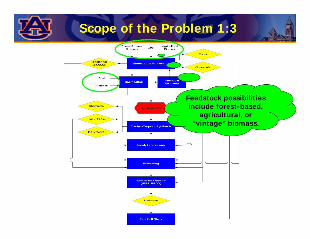
Feedstock possibilities include forest-based,
agricultural, or “vintage” biomass.
Scope of the Problem 1:3
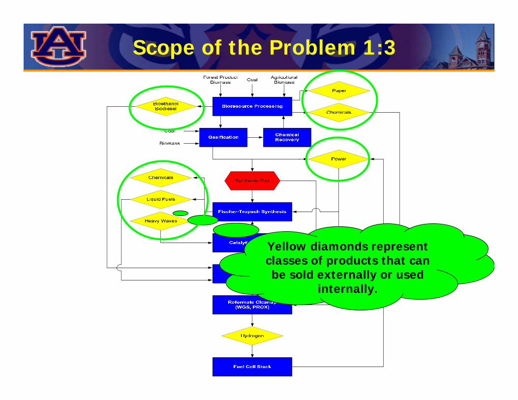
Yellow diamonds represent classes of products that can be sold externally or used
internally.

Scope of the Problem 1:3
Blue rectangles represent chemical
processes that may include
multiple subprocesses.
Scope of the Problem 1:3
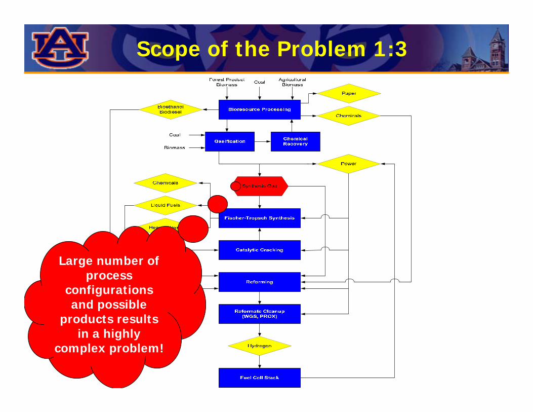
Large number of process
configurations and possible
products results in a highly
complex problem!

Scope of the Problem 2:3
• Complexity of the Problem– Large number of combinations of process configurations
as well as possible products results in a highly complex problem.
– Decision makers must be able to react to changes in market prices and environmental targets by identifying the optimal product distribution and process configuration.
– To assist decision makers in this process, it is necessary to develop a framework which includes environmental impact metrics, profitability measures, and other techno-economic metrics.

Scope of the Problem 3:3
• Framework should enable decision makers to answer the following questions:
– For a given set of product prices, what should the process configuration be? More specifically, what products should be produced in what amounts?
– What are the discrete product prices leading to switching between different production schemes?
– For a given set of desired products, what production route results in the lowest environmental impact?
– What are the ramifications of changes in supply chain conditions on the optimal process configuration?

Project Objectives 1:1
• Project Objectives– Utilize systematic methods to identify optimal product
allocation and processing routes for the emerging field of biorefining
– Incorporate environmental impact assessment in the design procedure and decision-making process
– Enhance understanding of the global interactions between the subprocesses and how they impact environmental, technical, and economic performance
– Incorporate solution into larger problem concerning biorefinery logistics in order to develop a greater understanding concerning the life cycle of biorefining

Problem Approach 1:2
Develop superstructure of
feasible biorefining possibilities for a given
feedstock.

Initial Superstructure Generation 1:3
• Feedstock to Product Approach– Given a feedstock, determine possible products
– Existing equipment– Available technology– Supply chain considerations
– Determine possible pathways to manufacture products– Evaluate salability of products or their possible use as
intermediates for value-added products
Initial Superstructure Generation 2:3
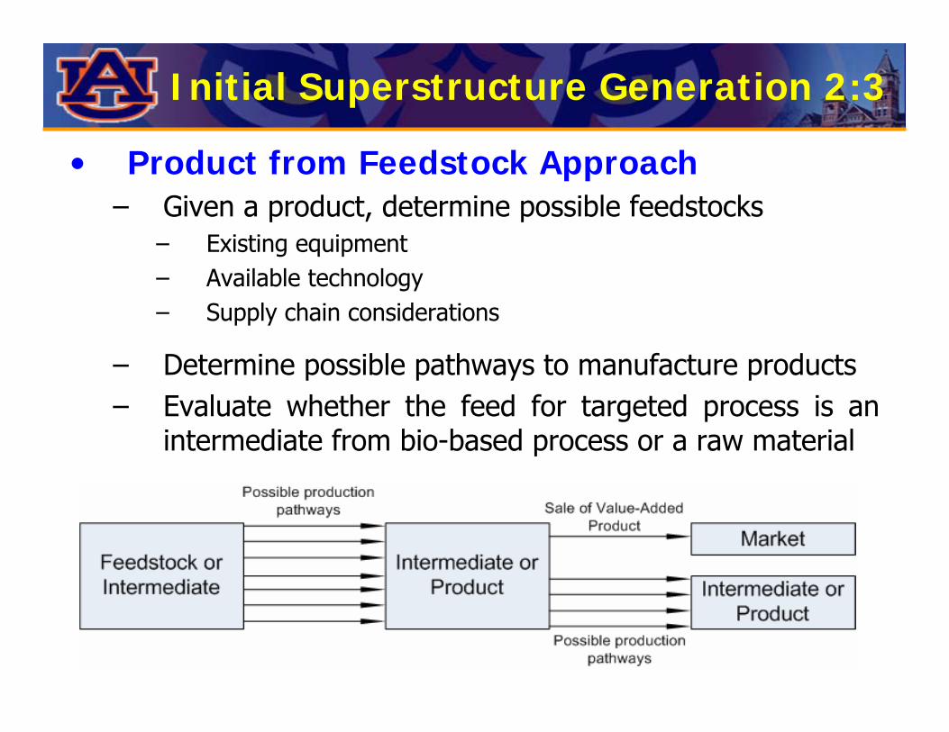
• Product from Feedstock Approach– Given a product, determine possible feedstocks
– Existing equipment– Available technology– Supply chain considerations
– Determine possible pathways to manufacture products– Evaluate whether the feed for targeted process is an
intermediate from bio-based process or a raw material
Initial Superstructure Generation 3:3
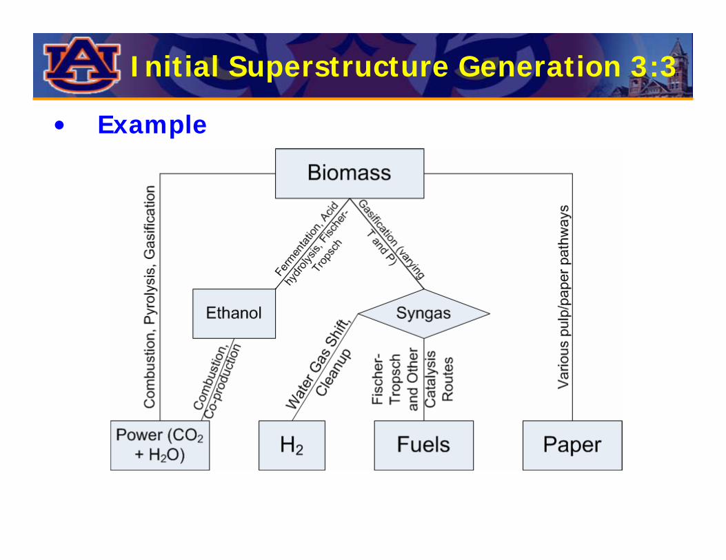
• Example
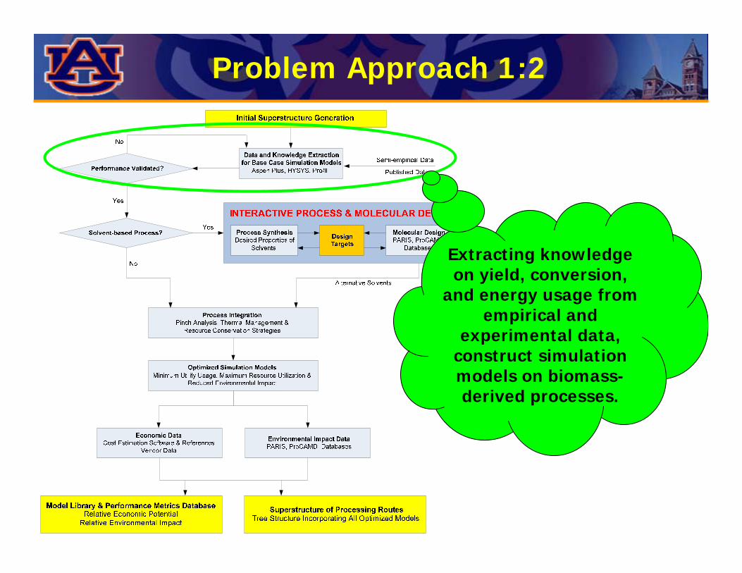
Problem Approach 1:2
Extracting knowledge on yield, conversion,
and energy usage from empirical and
experimental data, construct simulation models on biomass-derived processes.

Basic Simulation Models 1:3
• For basic simulation models– Develop all models on a consistent basis
– Terms of feedstock flow or desired product flow– Run at consistent percentage of capacity (e.g. 80%)
– Note main equipment needed– Preparation, main process, separation– Use black box models if details are unavailable
– Limit number of process combinations– Use “high” or “low” temperature/pressure instead of a range of
different operating temperature/pressures– Look at using different classes of catalysts instead of numerous
individual ones
Basic Simulation Models 2:3
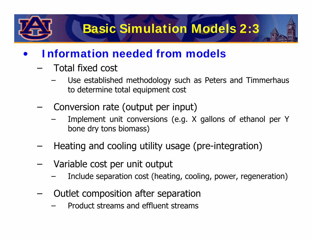
• Information needed from models– Total fixed cost
– Use established methodology such as Peters and Timmerhausto determine total equipment cost
– Conversion rate (output per input)– Implement unit conversions (e.g. X gallons of ethanol per Y
bone dry tons biomass)
– Heating and cooling utility usage (pre-integration)
– Variable cost per unit output– Include separation cost (heating, cooling, power, regeneration)
– Outlet composition after separation– Product streams and effluent streams

Basic Simulation Models 3:3
• Black box advantages– Speed and simplicity
– Ability to tackle more process configurations at once
– May evaluate newer technologies in which details are not yet available
• Detailed model advantages– More robust solutions
– Potential to uncover hidden inefficiencies in details
– Ability to utilize process integration in order to decrease variable and fixed costs
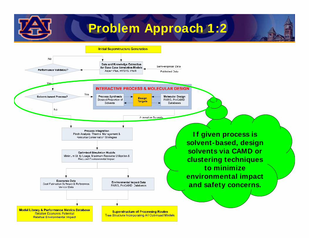
Problem Approach 1:2
If given process is solvent-based, design solvents via CAMD or clustering techniques
to minimize environmental impact and safety concerns.
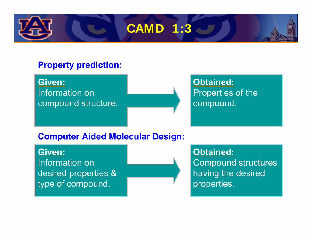
CAMD 1:3

CAMD 2:3
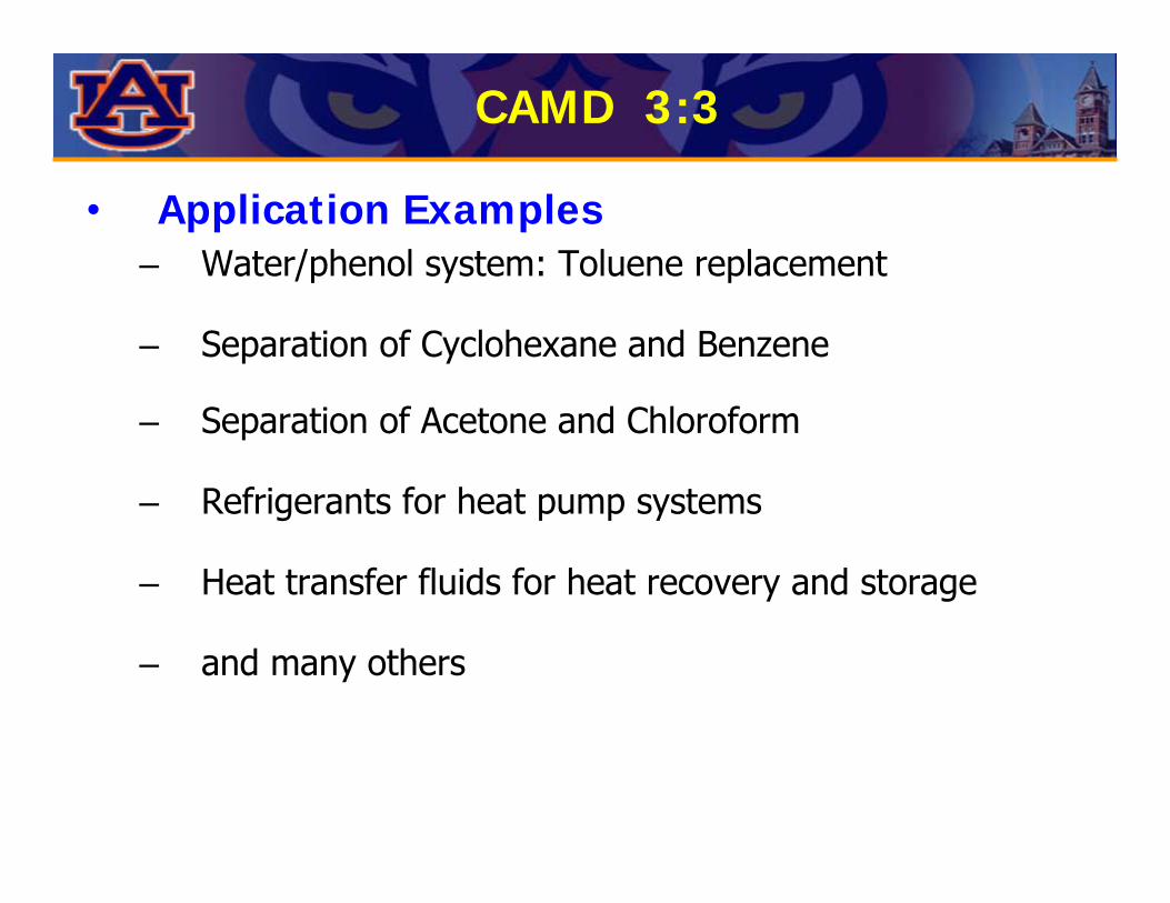
CAMD 3:3
• Application Examples– Water/phenol system: Toluene replacement
– Separation of Cyclohexane and Benzene
– Separation of Acetone and Chloroform
– Refrigerants for heat pump systems
– Heat transfer fluids for heat recovery and storage
– and many others

Aniline Case Study 1:7
• Problem Description– During the production of a pharmaceutical, aniline is
formed as a byproduct. Due to strict product specifications the aniline content of an aqueous solution has to be reduced from 28000 ppm to 2 ppm.
• Conventional Approach– Single stage distillation.– Reduces aniline content to 500 ppm. – Energy usage: 4248.7 MJ– No data is available for the subsequent downstream
processing steps.

Aniline Case Study 2:7
• Objective– Investigate the possibility of using liquid-liquid
extraction as an alternative unit operation by identification of a feasible solvent
• Reported Aniline Solvents– Water, Methanol, Ethanol, Ethyl Acetate, Acetone
Property Aniline Water CAS No. 62–53–3 7732–18–5
Boiling Point (K) 457.15 373.15 Solubility Parameter (MPa½) 24.12 47.81

• Performance of Solvent– Liquid at ambient temperature– Immiscible with water– No azeotropes between solvent & aniline and/or water– High selectivity with respect to aniline– Minimal solvent loss to water phase– Sufficient difference in boiling points for recovery
• Structural and EH&S Aspects– No phenols, amines, amides or polyfunctional
compounds.– No compounds containing double/triple bonds.– No compounds containing Si, F, Cl, Br, I or S
Aniline Case Study 3:7

Aniline Case Study 4:7
• Results of Solvent Search– No high boiling solvents found
Also, higher and branched alkaneswere identified as
candidates
Solvent CAS No. n-Octane 111–65–9
2-Heptanone 110–43–0 3-Heptanone 106–35–4

Aniline Case Study 5:7
• Process Simulation
1
2
3
4
5
6
7
8
9
10
11
12
13
14
15
T2
23456789
101112131415161718192021222324
1
25T1
S1
S3
S4
S2
S5
S6Aniline Laden Water
Solvent
Water (2 ppm Aniline)
Aniline Laden Solvent
Recovered Aniline
Recovered Solvent
Ext
ract
ion
Col
umn
Reg
ener
atio
n C
olum
n
(15
Sta
ges)
(25
Sta
ges)

Aniline Case Study 6:7
• Performance Targets and Results– Countercurrent extraction and simple distillation.– Terminal concentration of 2 ppm aniline in water phase.– Highest possible purity during solvent regeneration
Design Parameter n-Octane 2-Heptanone 3-HeptanoneSolvent amount (mole) 2488.8 1874.0 1873.5
Solvent amount (kg) 284.3 214.0 213.9 Solvent amount (liter) 402.6 261.2 260.9
Solvent amount in water phase (mol) 0.0341 161.2 161.2 Solvent amount in water phase (ppm) 1 429 429
Aniline product purity (weight%) 100.00 100.00 100.00 Recovery of aniline from solvent (%) 100.00 99.95 99.99
Solvent loss (% on a mole basis) 0.00098 8.60 8.60 Energy consumption for solvent recovery 2.223 2.245 2.009
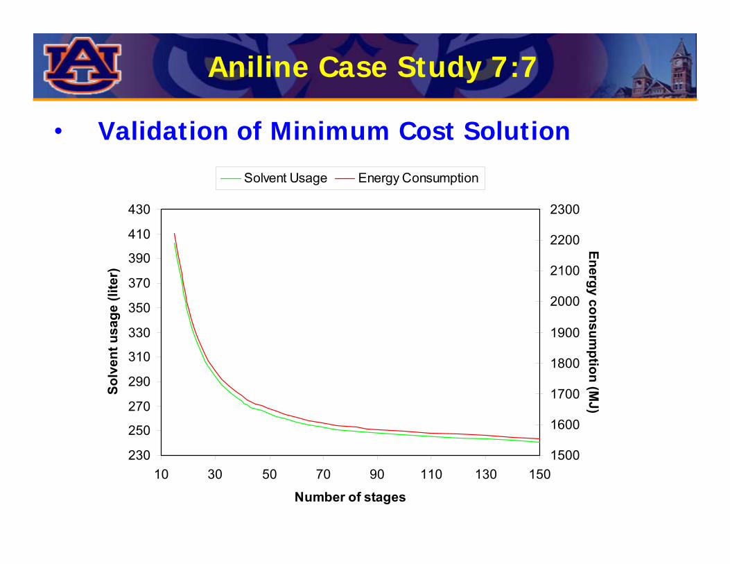
Aniline Case Study 7:7
• Validation of Minimum Cost Solution
230
250
270
290
310
330
350
370
390
410
430
10 30 50 70 90 110 130 150
Number of stages
Solv
ent u
sage
(lite
r)
1500
1600
1700
1800
1900
2000
2100
2200
2300
Energy consumption (M
J)
Solvent Usage Energy Consumption

Oleic Acid Methyl Ester 1:3
• Problem Description– Fatty acid used in a variety of applications, e.g. textile
treatment, rubbers, waxes, and biochemical research
– Reported solvents: Diethyl Ether, Chloroform
• Goal– Identify alternative solvents with better safety and
environmental properties.
VolatileFlammable Carcinogen

Oleic Acid Methyl Ester 2:3
• Solvent Specification– Liquid at normal (ambient) operating conditions.– Non-aromatic and non-acidic (stability of ester).– Good solvent for Oleic acid methyl ester.
• Constraints– Melting Point (Tm) < 280K– Boiling Point (Tb) > 340K– Acyclic compounds containing no Cl, Br, F, N or S– Octanol/Water Partition coefficient (logP) < 2– 15.95 (MPa)½ < δ < 17.95 (MPa)½
Oleic Acid Methyl Ester 3:3
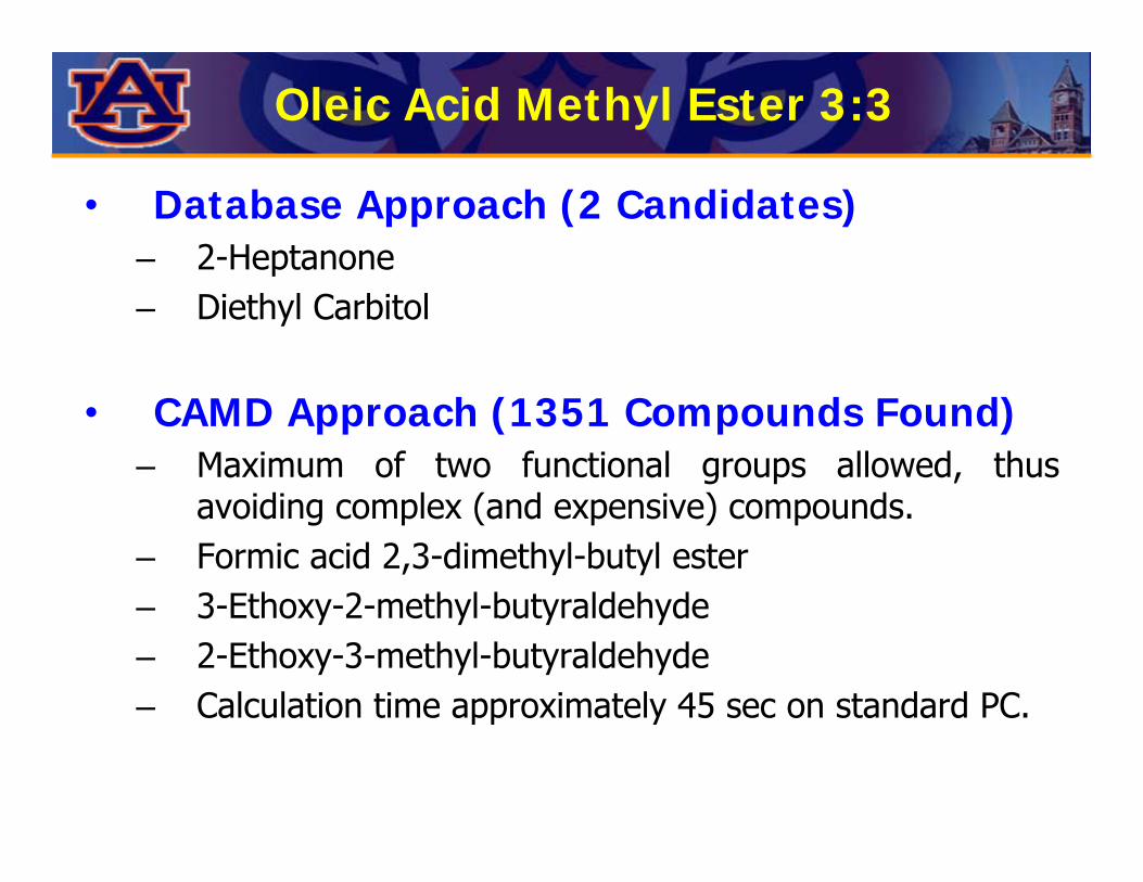
• Database Approach (2 Candidates)– 2-Heptanone– Diethyl Carbitol
• CAMD Approach (1351 Compounds Found)– Maximum of two functional groups allowed, thus
avoiding complex (and expensive) compounds.– Formic acid 2,3-dimethyl-butyl ester– 3-Ethoxy-2-methyl-butyraldehyde– 2-Ethoxy-3-methyl-butyraldehyde– Calculation time approximately 45 sec on standard PC.
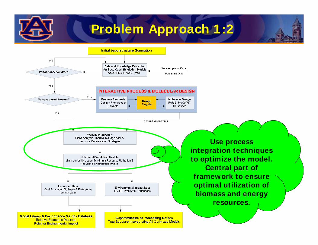
Problem Approach 1:2
Use process integration techniques to optimize the model.
Central part of framework to ensure optimal utilization of biomass and energy
resources.
Heat Integration Overview
• Early pioneers – Rudd @ Wisconsin (1968) – Hohmann @ USC (1971)
• Central figure – Linnhoff @ ICI/UMIST (1978)– Currently: President, Linnhoff-March
• Recommended text– Seider, Seader and Lewin (2004): Product and Process Design
Principles, 2 ed. Wiley and Sons, NY– Linnhoff et al. (1982): A User Guide on Process Integration for
the Efficient Use of Energy, I. Chem. E., London
• Most comprehensive review:– Gundersen, T. and Naess, L. (1988): The Synthesis of Cost
Optimal Heat Exchanger Networks: An Industrial Review of the State of the Art, Comp. Chem. Eng., 12(6), 503-530
Heat Integration Basics
• The design of Heat Exchanger Networks (HENs) deals with the following problem:
Given:
NH hot streams, with given heat capacity flowrate, each having to be cooled from supply temperature TH
S to targets THT
NC cold streams, with given heat capacity flowrate, each having to be heated from supply temperature TC
S to targets TCT
Design:
An optimum network of heat exchangers, connecting between the hot and cold streams and between the streams and cold/hot utilities (furnace, hot-oil, steam, cooling water or refrigerant, depending on the required duty temperature)
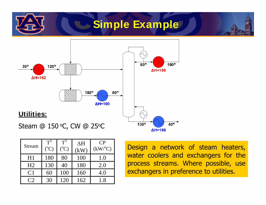
Simple Example
Stream TS
(oC) TT
(oC) ΔH(kW)
CP(kW/oC)
H1 180 80 100 1.0 H2 130 40 180 2.0 C1 60 100 160 4.0 C2 30 120 162 1.8
Design a network of steam heaters, water coolers and exchangers for the process streams. Where possible, use exchangers in preference to utilities.
Utilities:
Steam @ 150 oC, CW @ 25oC

Simple Example - Targets
130°
Units: 4Steam: 60 kWCooling water: 18 kW
Are these numbers optimal??

The Composite Curve 1:2Temperature
Enthalpy
T1
T2
T3
T4
T5
C P =
A
CP = B
C P =
C
H Interval
(T1 - T2)*B
(T2 - T3)*(A+B+C)
(T3 - T4)*(A+C)
(T4 - T5)*A
Three (3) hot streams

The Composite Curve 2:2
Three (3) hot streams

H=150
H
180
130
CP = 3.0
80
40
H=50
H=80
C P =
1.0
C P = 2.0
T
Simple Ex. – Hot Composite
H=150
T
H
180
130
C P =
1.0
C P = 2.0
80
40
H=50
H=80Not to scale!!
Not to scale!!

H=232
T
H
120
100
CP = 5.8
60
30
H=36
H=54
C P =
1.8
C P =
1.8
Simple Ex. – Cold Composite
H=232
T
H
120
100
C P =
1.8
CP = 4.0
60
30
H=36
H=54Not to scale!!
Not to scale!!
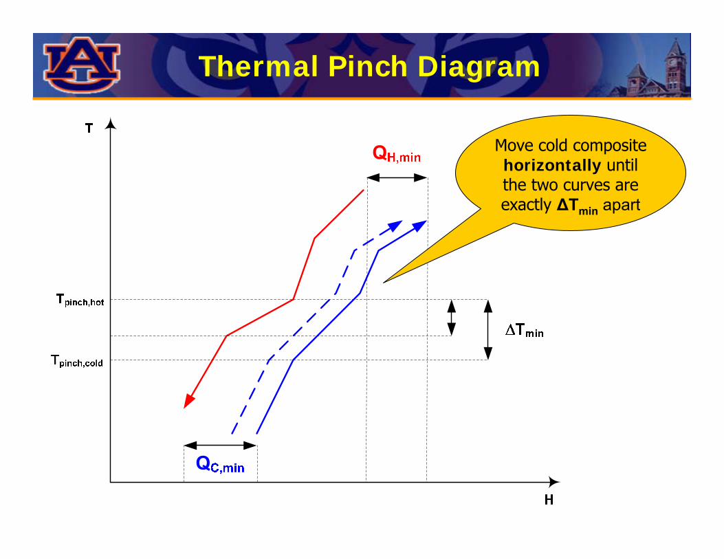
Thermal Pinch Diagram
Move cold composite horizontally until the two curves are exactly ΔTmin apart

Simple Ex. - Pinch Diagram
020406080
100120140160180200
0 50 100 150 200 250 300 350
Enthalpy
Tem
pera
ture
QCmin = 6 kW QHmin = 48 kW
TCpinch = 60
THpinch = 70
Maximum Energy Recovery (MER) Targets!

The Pinch
The “pinch” separates the HEN problem into two parts:
Heat sink - above the pinch, where at least QHmin utility must be usedHeat source - below the pinch, where at least QCmin utility must be used.
H
T
QCmin
QHmin
“PINCH”
H
T
QCmin
QHmin
HeatSource Heat
Sink
ΔTmin
+x
x
+x

Significance of the Pinch
• Do not transfer heat across pinch
• Do not use cold utilities above the pinch
• Do not use hot utilities below the pinch

Algebraic Targeting Method
• Temperature scales– Hot stream temperatures (T)– Cold stream temperatures (t)
• Thermal equilibrium– Achieved when T = t
• Inclusion of temperature driving force ΔTmin– T = t + ΔTmin
– Thus substracting ΔTmin from the hot temperatures will ensure thermal feasibility at all times

Algebraic Targeting Method
• Exchangeable load of the u’th hot stream passing through the z’th temperature interval:
• Exchangeable capacity of the v’th cold stream passing through the z’th temperature interval:
, 1( )Hu z u z zQ C T T−= −
, 1 1 min min
, 1
( ) (( ) ( ))
( )
Cv z v z z v z z
Cv z v z z
Q C t t C T T T T
Q C T T
− −
−
= − = −Δ − −Δ
= −
c

Algebraic Targeting Method
• Collective load of the hot streams passing through the z’th temperature interval is:
• Collective capacity of the cold streams streamspassing through the z’th temperature interval is:
,H Hz u z
uH QΔ =∑
,C Cz v z
uH QΔ =∑
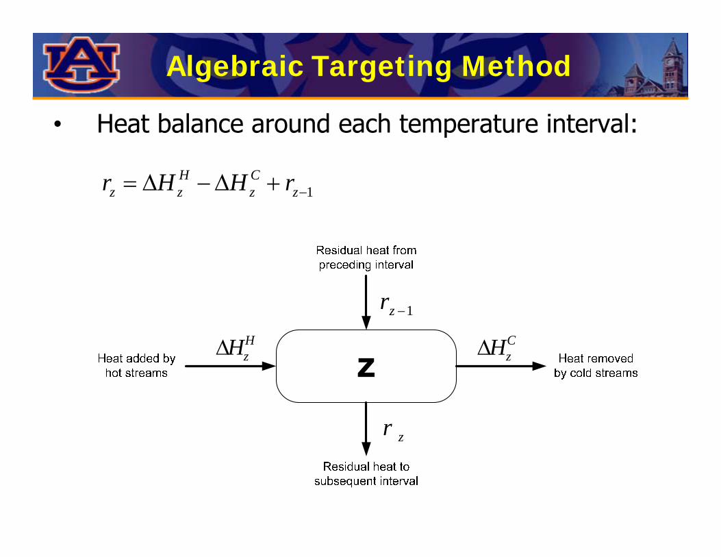
Algebraic Targeting Method
• Heat balance around each temperature interval:
1H C
z z z zr H H r −= Δ −Δ +
HzHΔ
1zr −
CzHΔ
zr
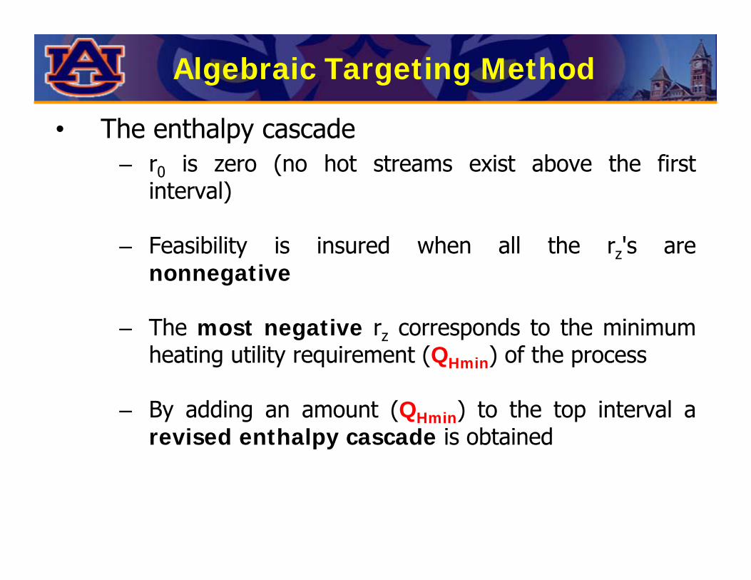
Algebraic Targeting Method
• The enthalpy cascade– r0 is zero (no hot streams exist above the first
interval)
– Feasibility is insured when all the rz's are nonnegative
– The most negative rz corresponds to the minimum heating utility requirement (QHmin) of the process
– By adding an amount (QHmin) to the top interval a revised enthalpy cascade is obtained

Algebraic Targeting Method
• The revised enthalpy cascade– On the revised cascade the location of rz=0
corresponds to the heat-exchange pinch point
– Overall energy balance for the network must be realized, thus the residual load leaving the last temperature interval is the minimum cooling utility requirement (QCmin) of the process

Mass Exchange Networks 1:4
MassExchange Network
MSA’s (Lean Streams In)
RichStreamsIn
RichStreamsOut
MSA’s (Lean Streams Out)

Mass Exchange Networks 2:4
• What do we know?– Number of rich streams (NR)– Number of process lean streams or process MSA’s (NSP)– Number of external MSA’s (NSE)
– Rich stream data• Flowrate (Gi), supply (yi
s) and target compositions (yit)
– Lean stream (MSA) data• Supply (xj
s) and target compositions (xjt)
• Flowrate of each MSA is unknown and is determined as to minimize the network cost
Mass Exchange Networks 3:4
• Synthesis Tasks– Which mass-exchange operations should be used (e.g.,
absorption, adsorption, etc.)?
– Which MSA's should be selected (e.g., which solvents, adsorbents, etc.)?
– What is the optimal flowrate of each MSA?
– How should these MSA's be matched with the rich streams (i.e., stream parings)?
– What is the optimal system configuration?

Mass Exchange Networks 4:4
• Classification of Candidate Lean Streams (MSA’s)– NSP Process MSA’s– NSE External MSA’s
• Process MSA’s– Already available at plant site– Can be used for pollutant removal virtually for free– Flowrate is bounded by availability in the plant
• External MSA’s– Must be purchased from market– Flowrates determined according to overall economics
NS = NSP + NSE

Mass Integration Overview
• Pinch Diagram– Useful tool for representing global transfer of mass– Identifies performance targets, e.g. MOC– Has accuracy problems for problems with wide ranging
compositions or many streams
• Algebraic Method– No accuracy problems– Can handle many streams easily– Can be programmed and formulated as optimization
problems
Algebraic Mass Integration 1:7
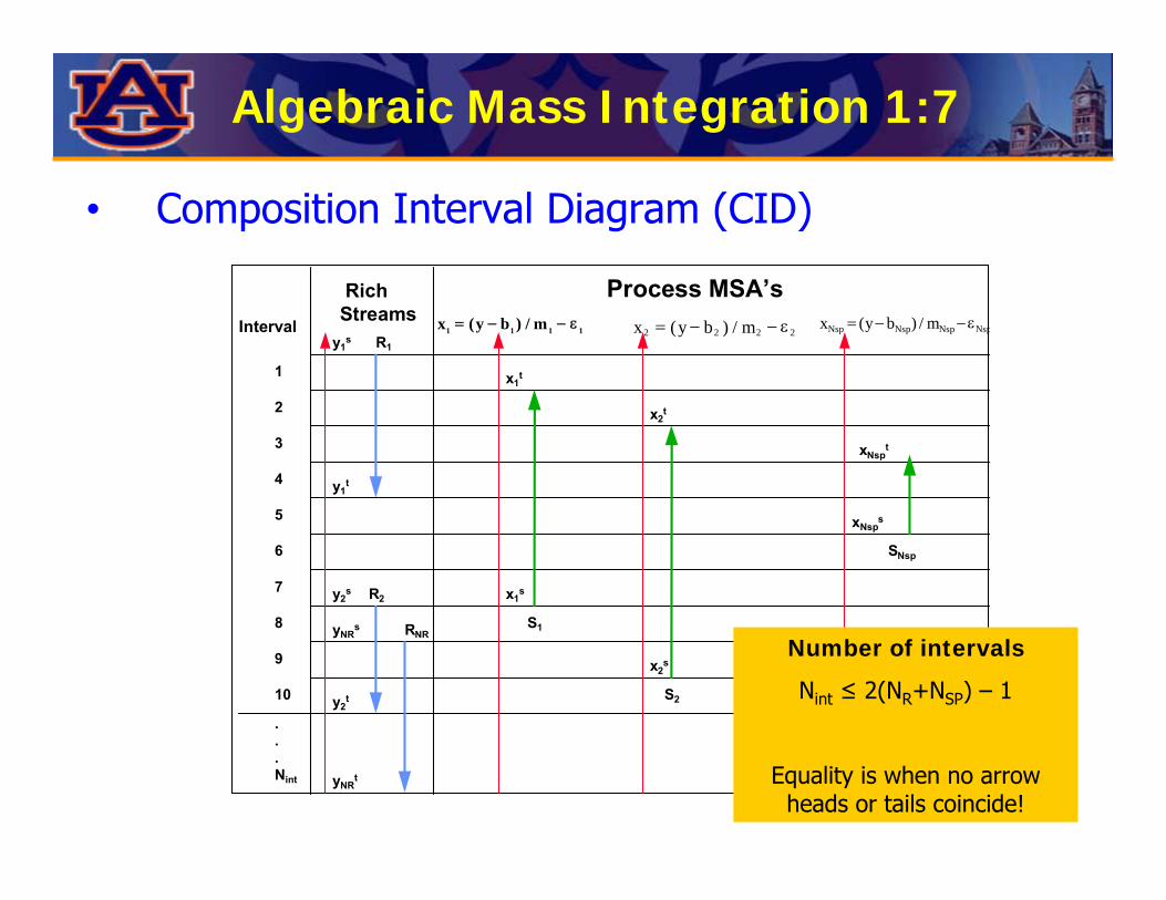
• Composition Interval Diagram (CID)
Interval
RichStreams
Process MSA’sx y b m1 1 1 1= − −( ) / ε x y b m2 2 2 2= − −( ) / ε x y b mNsp Nsp Nsp Nsp= − −( ) / ε
1
2
3
4
5
6
7
8
9
10
.
.
.Nint
y1s R1
y1t
y2s
yNRs
y2t
yNRt
R2
RNR
x1t
x1s
S1
S2
x2t
x2s
xNspt
xNsps
SNsp
Number of intervals
Nint ≤ 2(NR+NSP) – 1
Equality is when no arrow heads or tails coincide!
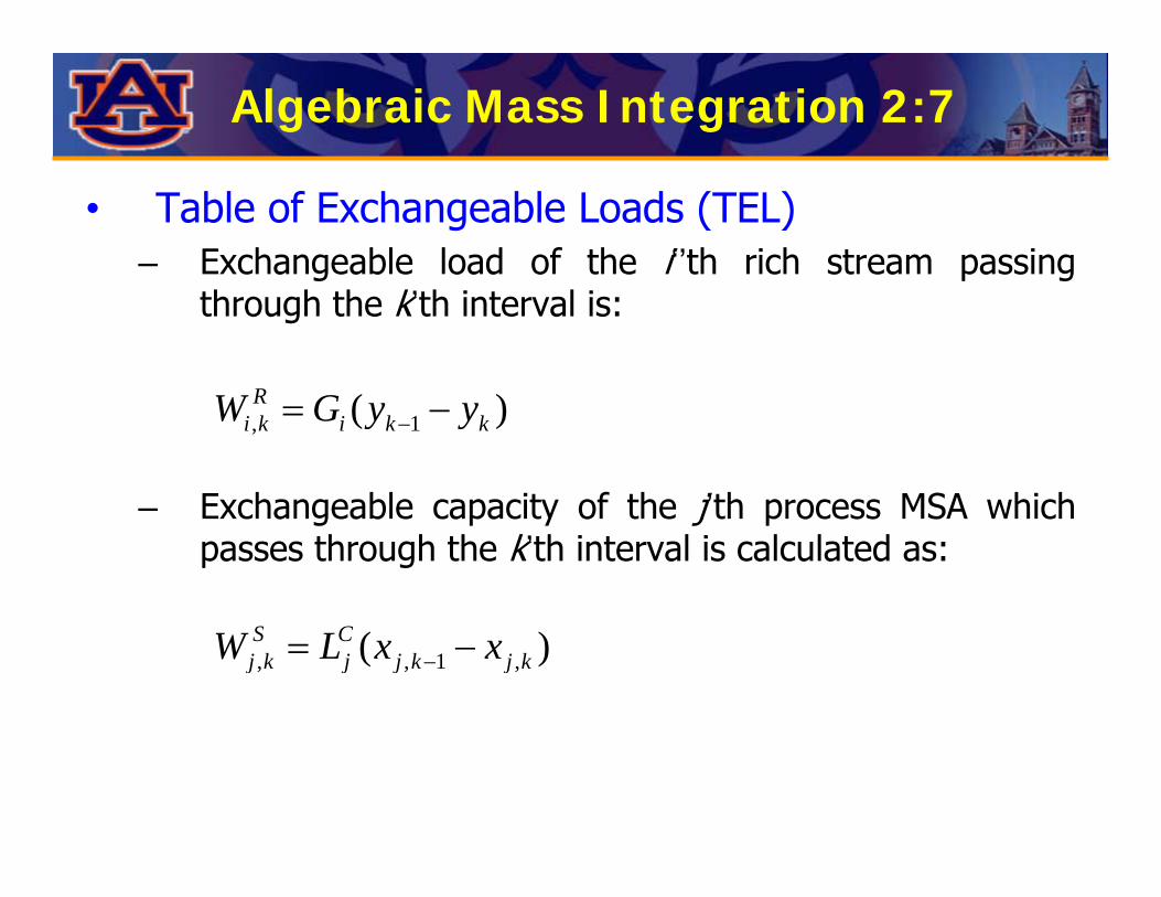
• Table of Exchangeable Loads (TEL)– Exchangeable load of the i‘’th rich stream passing
through the k’th interval is:
– Exchangeable capacity of the j’th process MSA which passes through the k’th interval is calculated as:
Algebraic Mass Integration 2:7
, 1( )Ri k i k kW G y y−= −
, , 1 ,( )S Cj k j j k j kW L x x−= −

• Table of Exchangeable Loads (TEL) (Cont’d)– Collective load of the rich streams passing through the
k’th interval is:
– Collective capacity of the lean streams passing through the k’th interval is:
Algebraic Mass Integration 3:7
, passes through interval
R Rk i k
i kW W= ∑
, passes through interval
S Sk j k
j kW W= ∑
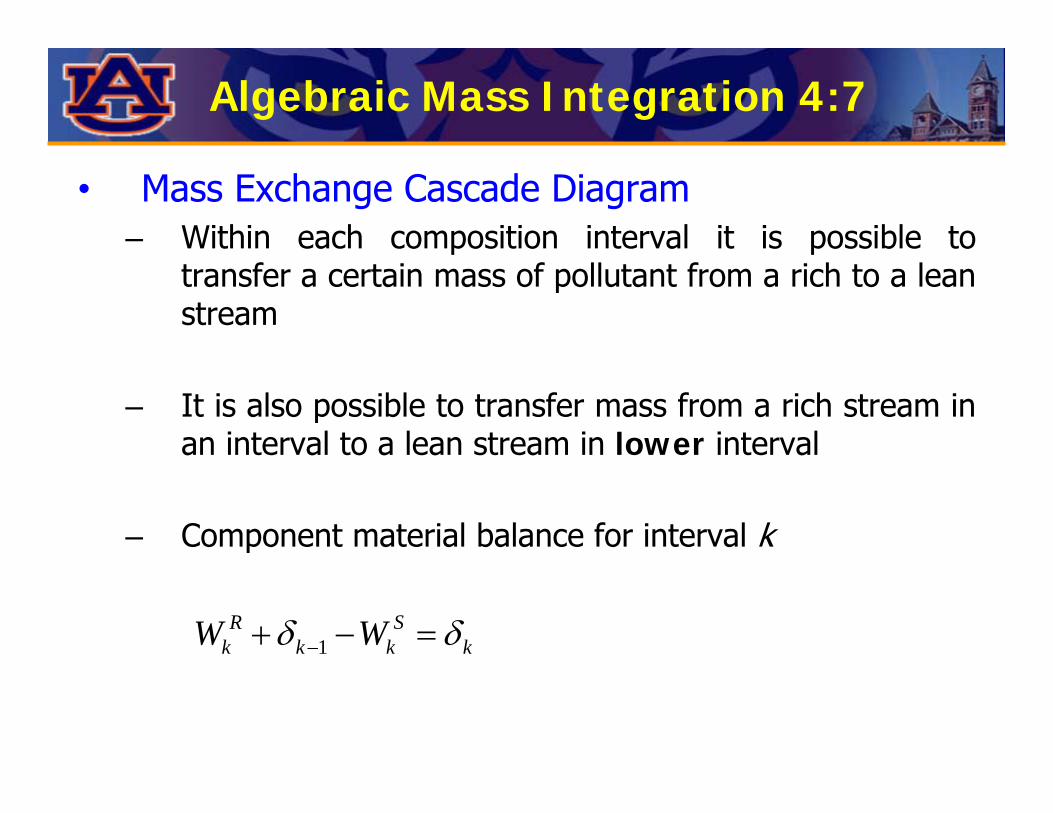
• Mass Exchange Cascade Diagram– Within each composition interval it is possible to
transfer a certain mass of pollutant from a rich to a lean stream
– It is also possible to transfer mass from a rich stream in an interval to a lean stream in lower interval
– Component material balance for interval k
Algebraic Mass Integration 4:7
1R S
k k k kW Wδ δ−+ − =

• Mass Exchange Cascade Diagram (Cont’d)
Algebraic Mass Integration 5:7
kWkR Wk
S
δ k-1
δ k
Mass Recoveredfrom Rich
Streams
Mass Transferredto MSA’s
Residual Mass fromPreceeding Interval
Residual Mass toSubsequent Interval

Algebraic Mass Integration 6:7
• Comments– δ0 is zero (no rich streams exist above the first interval)
– Feasibility is insured when all the δk's are nonnegative
– The most negative δk corresponds to the excess capacity of the process MSA's in removing the targeted species.
– After removing the excess capacity of MSA's, one can construct a revised TEL/cascade diagram in which the flowrates and/or outlet compositions of the process MSA's have been adjusted.

Algebraic Mass Integration 7:7
• Comments (Continued)– On the revised cascade diagram the location of
residual mass = zero corresponds to the mass-exchange pinch composition.
– Since an overall material balance for the network must be realized, the residual mass leaving the lowest composition interval of the revised cascade diagram must be removed by external MSA's.
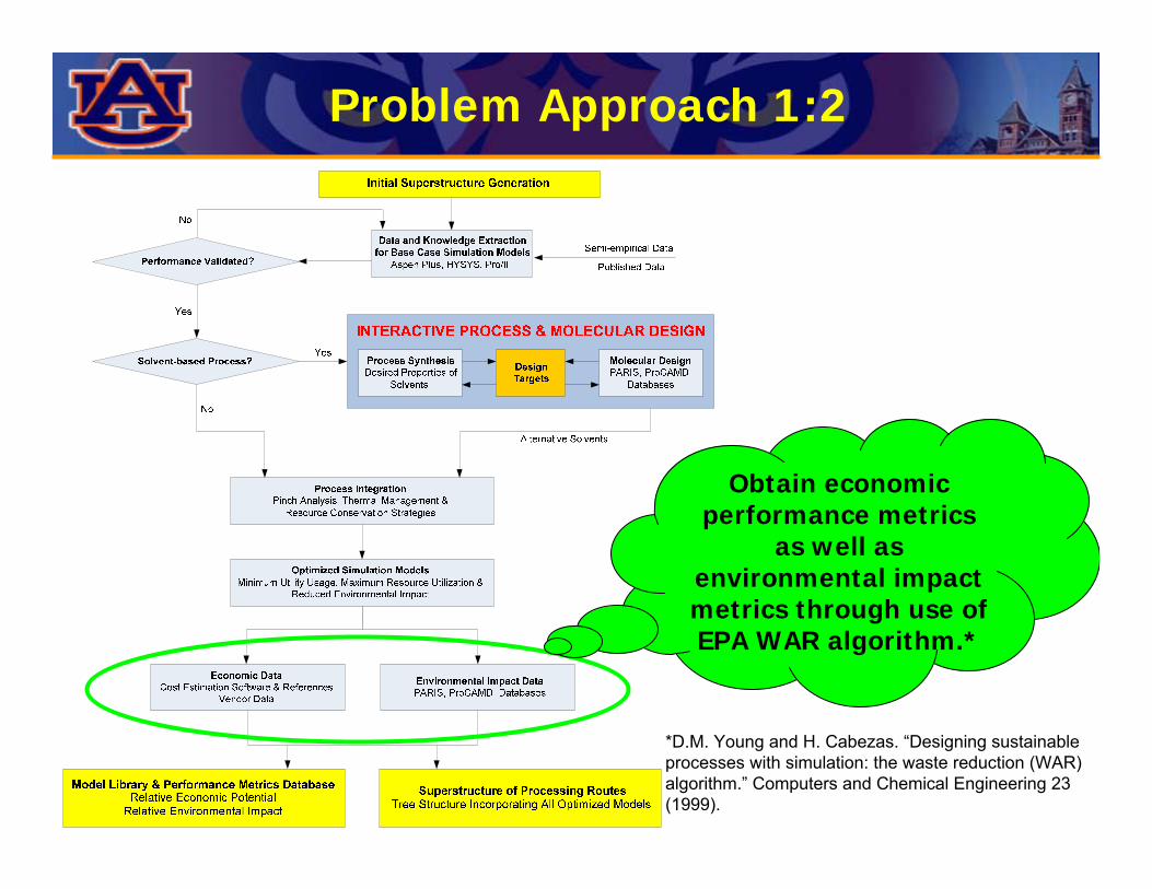
Problem Approach 1:2
Obtain economic performance metrics
as well as environmental impact metrics through use of EPA WAR algorithm.*
*D.M. Young and H. Cabezas. “Designing sustainable processes with simulation: the waste reduction (WAR) algorithm.” Computers and Chemical Engineering 23 (1999).

Economic Data 1:3
• Choose between two methods of measuring value:
– Gross profit (GP) method– Measures revenues minus costs over a fixed period of time
(basis of profit per hour, day, week, etc.)– No need for prediction of future economic conditions– Simplicity, ease of use, and reduced computational time
– Net present value (NPV) method– Measures net present value of decisions over a pre-determined
period of time (~10-20 years)– Takes into account the time value of money, current and
anticipated subsidy and incentive programs, and depreciation– Robust, with improved ability to quantify added value
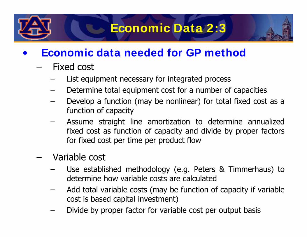
Economic Data 2:3
• Economic data needed for GP method– Fixed cost
– List equipment necessary for integrated process– Determine total equipment cost for a number of capacities– Develop a function (may be nonlinear) for total fixed cost as a
function of capacity– Assume straight line amortization to determine annualized
fixed cost as function of capacity and divide by proper factors for fixed cost per time per product flow
– Variable cost– Use established methodology (e.g. Peters & Timmerhaus) to
determine how variable costs are calculated– Add total variable costs (may be function of capacity if variable
cost is based capital investment)– Divide by proper factor for variable cost per output basis

Economic Data 3:3
• Economic data needed for NPV method– In addition to data needed for GP method:
– Window of time over which to calculate NPV– Estimated marginal tax rate at which decisions are taking place– Information on current and future tax credits and deductions,
subsidies, etc. for possible products or pathways– Probabilities on legislative courses of action which will impact
the economics of products or pathways– Time value of money interest rate– Acceptable depreciation method (MACRS vs. straight-line)– Depreciation schedules for specific equipment items, which
may vary– Monies dedicated to hedging against unfavorable market action
(e.g. options, futures, derivatives)
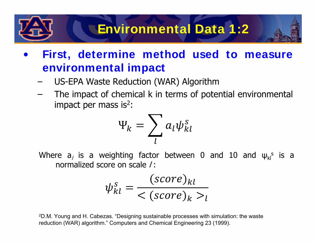
Environmental Data 1:2
• First, determine method used to measure environmental impact
– US-EPA Waste Reduction (WAR) Algorithm– The impact of chemical k in terms of potential environmental
impact per mass is2:
Where al is a weighting factor between 0 and 10 and ψkls is a
normalized score on scale l :
2D.M. Young and H. Cabezas. “Designing sustainable processes with simulation: the waste reduction (WAR) algorithm.” Computers and Chemical Engineering 23 (1999).

Environmental Data 2:2
• Next, look at individual criteria to be measured to determine what data is needed
– US-EPA Waste Reduction (WAR) Algorithm– Impact calculated by WAR Algorithm based on eight
criteria:
– Gather data from integrated models in order to determine scores
– Use of software and databases may decrease difficulty of determining environmental impact
Global warmingOzone depletionAcidificationPhotochemical oxidation
Human toxicity by ingestionHuman toxicity by inhalation or dermal exposureAquatic toxicityTerrestrial toxicity
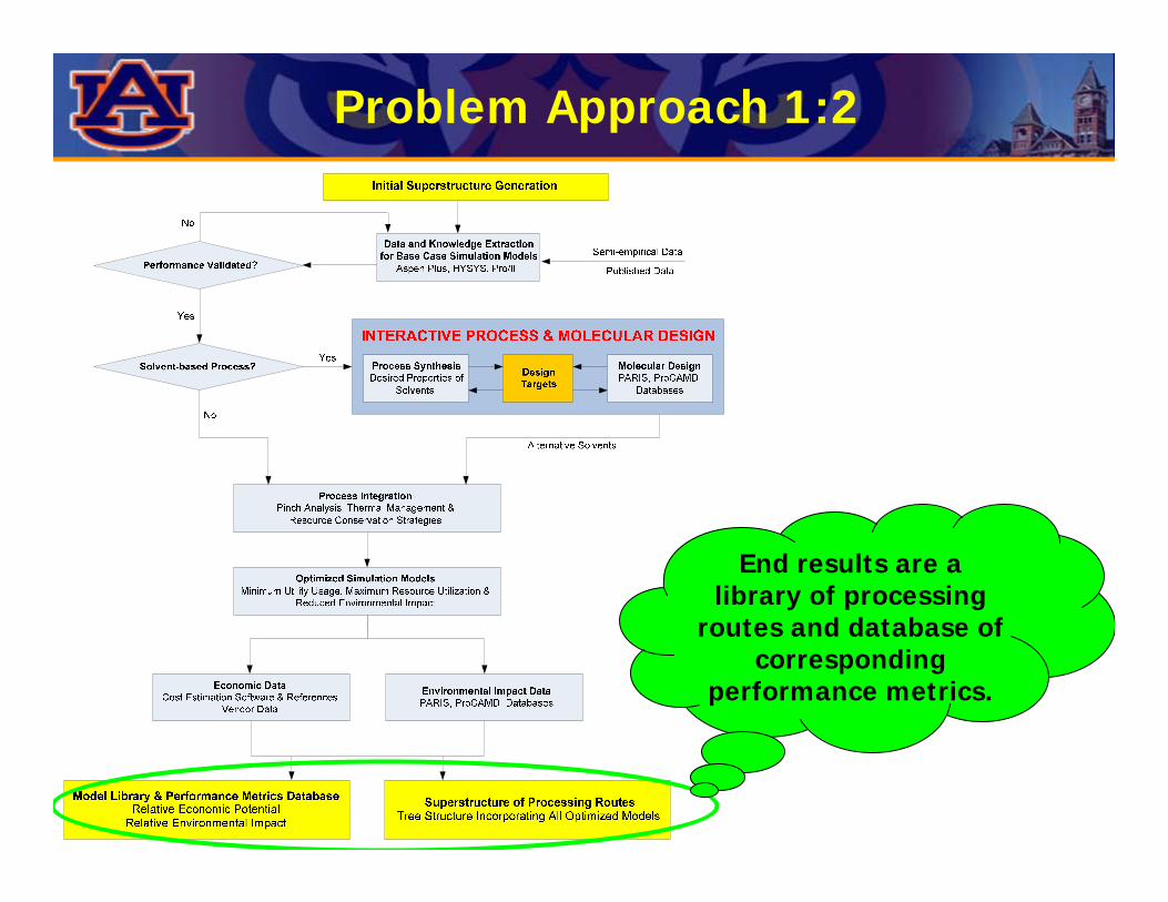
Problem Approach 1:2
End results are a library of processing
routes and database of corresponding
performance metrics.

Problem Approach 2:2
Combining the library of processing routes
and database of corresponding
performance metrics with a numerical
solver…

Problem Approach 2:2
…we arrive at a number of candidate
solutions that achieve optimal economic
performance.

General Model 1:1
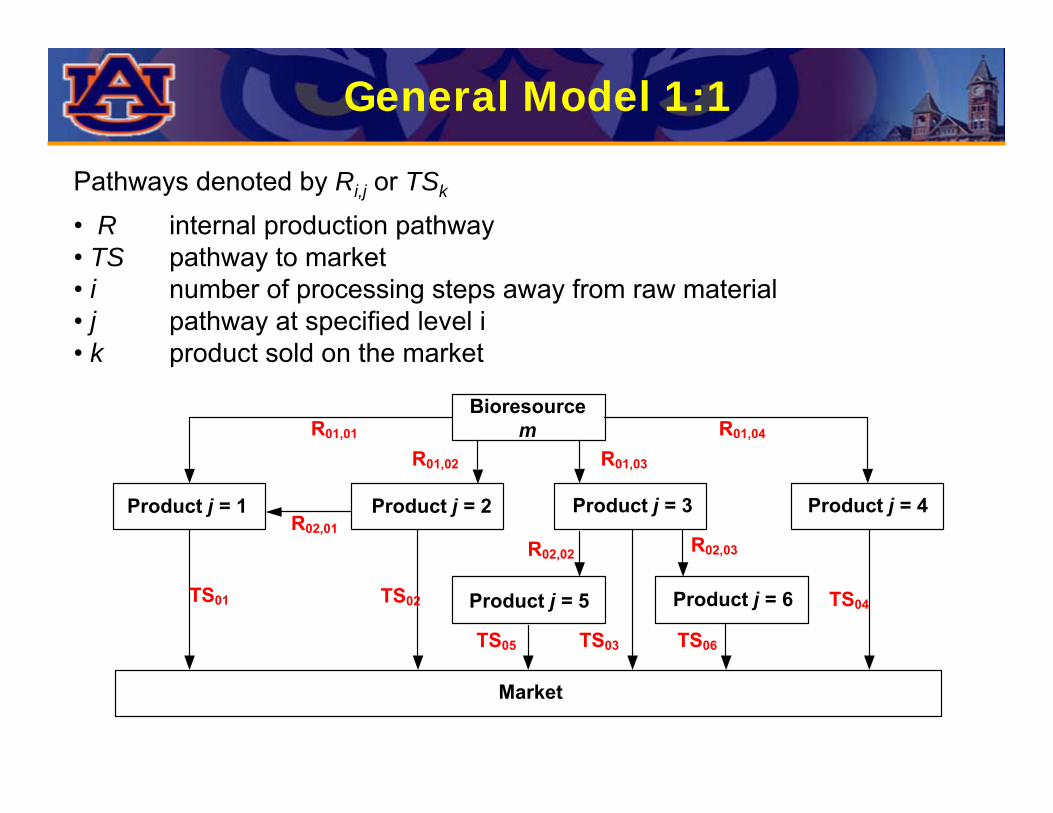
Pathways denoted by Ri,j or TSk
• R internal production pathway• TS pathway to market• i number of processing steps away from raw material• j pathway at specified level i• k product sold on the market
Bioresource m
Product j = 1 Product j = 2 Product j = 3 Product j = 4
Product j = 5 Product j = 6
R01,01 R01,04
R01,03R01,02
R02,01
R02,02 R02,03
Market
TS01 TS02
TS05 TS03 TS06
TS04

Economic Optimization 1:4
• Gross profit method
– TSk Amount of product k sold on the market– Ck
s Sales price of product k– Rmij Processing rate of route mij– Cmij
P Processing cost (fixed + variable) of route mij per unit output
– Rm1j Processing rate of bioresource m through route 1j– Cm
BM Purchase price of bioresource m

Economic Optimization 2:4
• Net present value method
– Taxt Marginal taxation rate in year t– Dept Depreciation amount in year t– Hedget Expenses (revenues) of hedging in year t– Govt Government incentives (penalties) in year t– TVM Time value of money (market rate of return)

Economic Optimization 3:4
• Constraints– Total capital investment, which dictates capacity
– Alternatively, maximum feasible capacity
– Maximum flowthrough based on capacity– Mass balances around the product points
– In * Conversion factor = To Sell + To Process + Waste
– Output composition– Energy balances– Biomass availability– Maximum output based on market and supply chain
conditions– Separations (purity, energy usage, size)
Economic Optimization 4:4
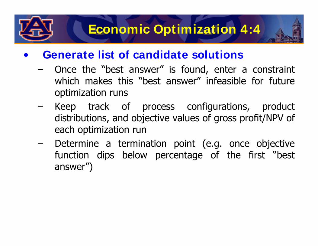
• Generate list of candidate solutions– Once the “best answer” is found, enter a constraint
which makes this “best answer” infeasible for future optimization runs
– Keep track of process configurations, product distributions, and objective values of gross profit/NPV of each optimization run
– Determine a termination point (e.g. once objective function dips below percentage of the first “best answer”)

Problem Approach 2:2
Using a measure of environmental impact
(e.g. EPA WAR), we rank candidate
solutions based on environmental impact.
General Model 1:1
Pathways denoted by Ri,j or TSk
• R internal production pathway• TS pathway to market• i number of processing steps away from raw material• j pathway at specified level i• k product sold on the market
Bioresource m
Product j = 1 Product j = 2 Product j = 3 Product j = 4
Product j = 5 Product j = 6
R01,01 R01,04
R01,03R01,02
R02,01
R02,02 R02,03
Market
TS01 TS02
TS05 TS03 TS06
TS04
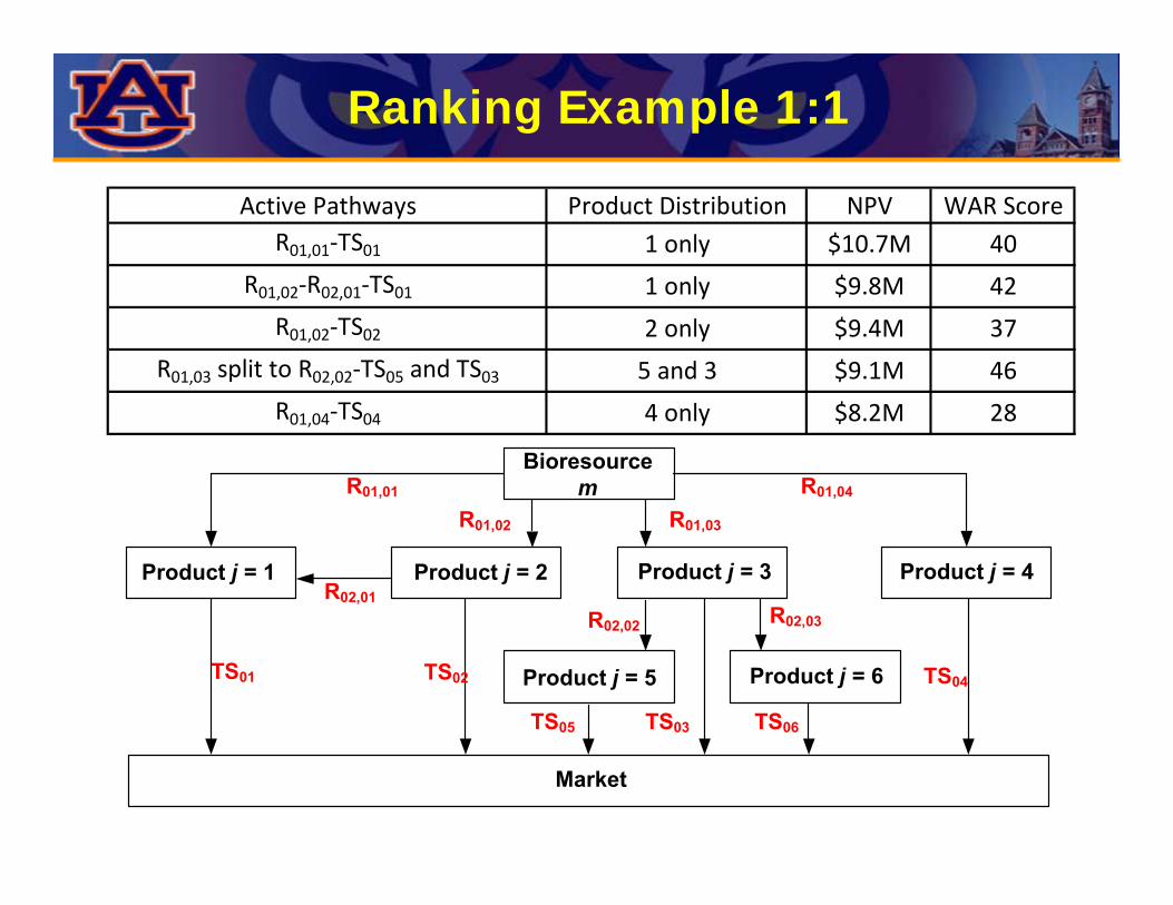
Ranking Example 1:1
Active Pathways Product Distribution NPV WAR ScoreR01,01‐TS01 1 only $10.7M 40
R01,02‐R02,01‐TS01 1 only $9.8M 42
R01,02‐TS02 2 only $9.4M 37
R01,03 split to R02,02‐TS05 and TS03 5 and 3 $9.1M 46
R01,04‐TS04 4 only $8.2M 28
Bioresource m
Product j = 1 Product j = 2 Product j = 3 Product j = 4
Product j = 5 Product j = 6
R01,01 R01,04
R01,03R01,02
R02,01
R02,02 R02,03
Market
TS01 TS02
TS05 TS03 TS06
TS04

Problem Approach 2:2
If environmental objectives are
satisfied, then we have arrived at the final
process design.
This methodology decouples the issues
of economic and environmental performance.
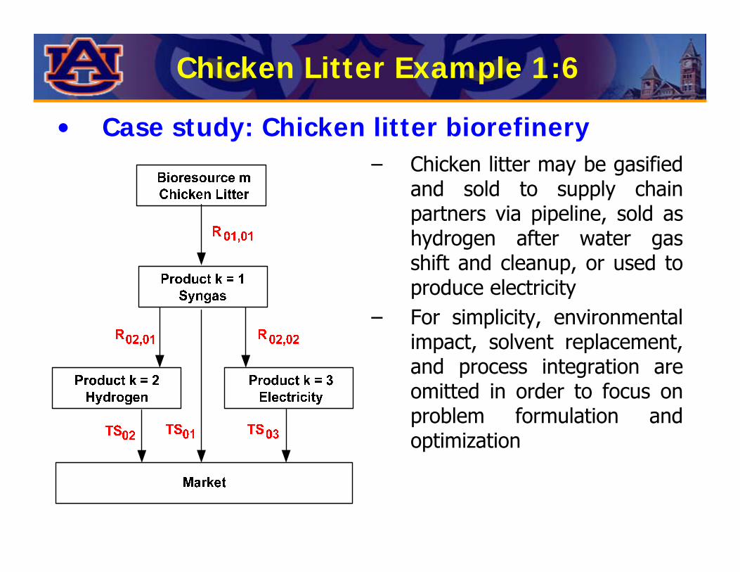
Chicken Litter Example 1:6
• Case study: Chicken litter biorefinery– Chicken litter may be gasified
and sold to supply chain partners via pipeline, sold as hydrogen after water gas shift and cleanup, or used to produce electricity
– For simplicity, environmental impact, solvent replacement, and process integration are omitted in order to focus on problem formulation and optimization
Chicken Litter Example 2:6
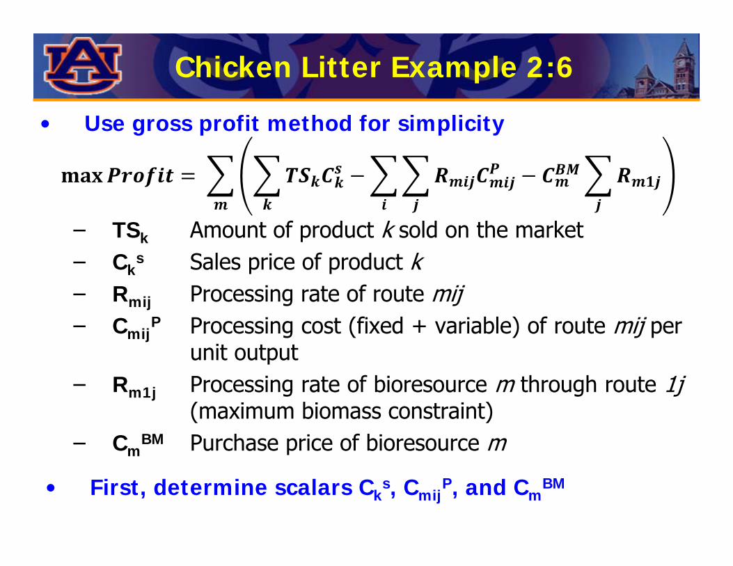
• Use gross profit method for simplicity
– TSk Amount of product k sold on the market– Ck
s Sales price of product k– Rmij Processing rate of route mij– Cmij
P Processing cost (fixed + variable) of route mij per unit output
– Rm1j Processing rate of bioresource m through route 1j (maximum biomass constraint)
– CmBM Purchase price of bioresource m
• First, determine scalars Cks, Cmij
P, and CmBM

Chicken Litter Example 3:6
• List equipment in order to determine fixed cost:Chicken Litter to Syngas Equipment Cost (2005 $K)
Air Separation Unit 52933Biomass Dryer 32523
Biomass Gasifier & Tar Cracker 18320Biomass Syngas Cooler and Filter 4998
Biomass Syngas expander 2661Feedstock Storage Area 867Total Fixed Cost (2005 $) $112,302,000
• Sum up variable cost factors:
Syngas to Electricity Equipment Cost (2005 $K)Combined Cycle Power Island
(details omitted) 100091Total Fixed Cost $100,091,000
Syngas to Hydrogen Equipment Cost (2005 $K)Syngas to H2 (details omitted) 461527
Total Fixed Cost $461,527,000
Litter to Syngas Cost Category Cost (2005 $)Utilities $96,541
Operating Labor $98,162 Operating Supervision $14,724
Maintenance $10,107,180 Operating Supplies $1,516,077 Laboratory Charges $14,724
Overhead $1,361,771 Administrative $408,531
Total Variable Cost $13,617,710.99
Syngas to Electricity Cost Category Cost (2005 $K)Electricity Purchases $5,893,707.90
Operation and Maintanance $9,407,549.48Total Variable Cost $15,301,257.39
Syngas to Hydrogen Cost Category Cost (2005 $)Utilities $127,943,849.88
Operating Labor $98,162Operating Supervision $14,724
Maintenance $41,537,405 Operating Supplies $6,230,611 Laboratory Charges $14,724
Overhead $20,211,434 Administrative $6,063,430
Total Variable Cost $202,114,340

Chicken Litter Example 4:6
• Add annualized fixed costs to variable costs to get Cmij
P:
• Find market prices for feedstock (CmBM) and
products (Cks):
Biomass to Syngas Syngas to Electicity Syngas to HydrogenTotal Fixed Cost $112,302,000 $100,091,000 $461,527,000Annualized Fixed Cost @ 8% interest over 25 years $10,401,000 $9,270,000 $42,745,000Total Variable Costs $13,618,000 $15,301,000 $202,114,000Total Annual Product Costs $24,019,000 $24,571,000 $244,859,000
Annual Output 4.018*108 kg 1.065*106 MWe 8957*108 m3
Cost per Output $0.0598/kg $23.07/MWe $0.273/m3
Market PriceChicken litter feedstock $0.010/kgSyngas $0.214/kgElectricity $53.370/MWe
Hydrogen $0.220/m3
• Perform optimization to determine products sold TSk and processing pathway amounts Rmij
Chicken Litter Example 5:6
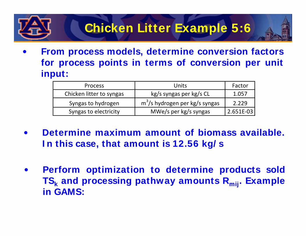
• From process models, determine conversion factors for process points in terms of conversion per unit input:
• Determine maximum amount of biomass available. In this case, that amount is 12.56 kg/s
• Perform optimization to determine products sold TSk and processing pathway amounts Rmij. Example in GAMS:
Process Units FactorChicken litter to syngas kg/s syngas per kg/s CL 1.057
Syngas to hydrogen m3/s hydrogen per kg/s syngas 2.229Syngas to electricity MWe/s per kg/s syngas 2.651E‐03
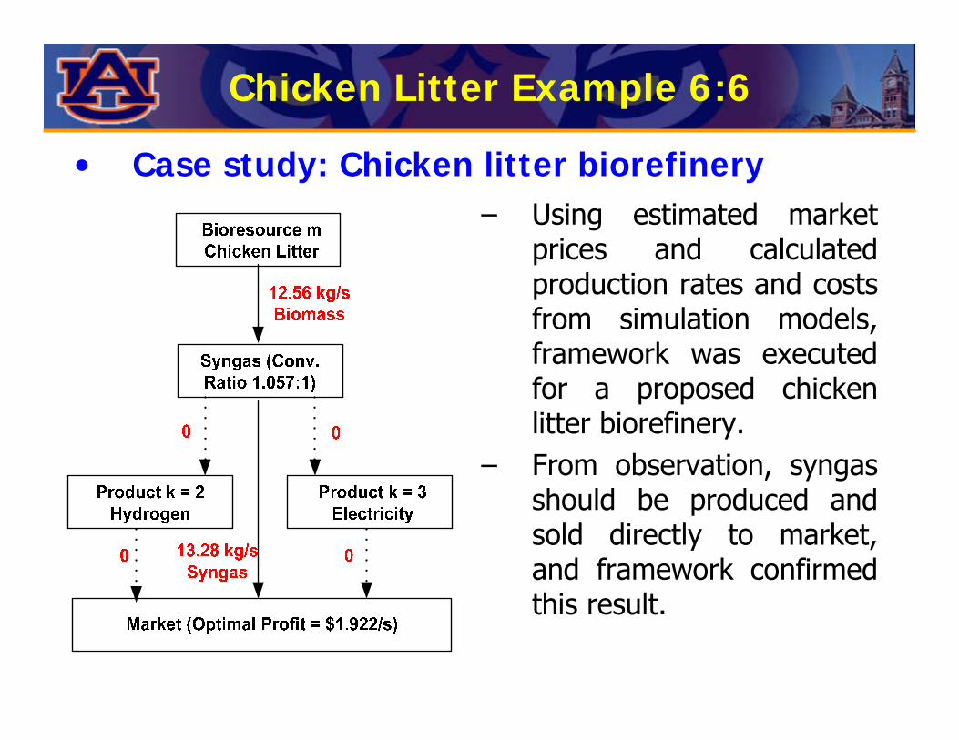
Chicken Litter Example 6:6
• Case study: Chicken litter biorefinery– Using estimated market
prices and calculated production rates and costs from simulation models, framework was executed for a proposed chicken litter biorefinery.
– From observation, syngas should be produced and sold directly to market, and framework confirmed this result.

Future Direction 1:1
– Continue increasing number of simulation models to generate processing costs, production rates, and data for environmental impact metrics
– Develop qualitative predictive models for capital investment as a function of processing rates
– Expand superstructures to include additional products and processes
– Enhance robustness of framework– Optimization under uncertainty– Alternative formulation methods
Acknowledgements
• Financial Support– NSF CAREER Program– US-EPA Science to Achieve Results (STAR)
Fellowship– Consortium for Fossil Fuel Science (CFFS)
• Industrial Collaborators– Masada Resource Group, LLC– Auburn Pulp and Paper Foundation– PureVision Technologies– Gas Technology Institute (GTI)

Further Information 1:3
– Bridgwater, A. V. (2003). Renewable fuels and chemicals by thermal processing of biomass. Chemical Engineering Journal, 91, 87-102
– Neathery, J.; Gray, D.; Challman, D. and Derbyshire, F. (1999). The pioneer plant concept: co-production of electricity and added-value products from coal. Fuel, 78, 815-823
– Slath, P. L. and Dayton, D. C. (2003). Preliminary Screening - Technical and Economic Assessment of Synthesis Gas to Fuels and Chemicals with Emphasis on the Potential for Biomass-Derived Syngas. Technical Report. NREL/TP-510-34929
– Dry, M. E. (1982). Catalytic Aspects of Industrial Fischer-Tropsch Synthesis. Journal of Molecular Catalysis, Volume 17, Issues 2-3, 133-144
– Dry, M. E. (1996). Practical and theoretical aspects of the catalytic Fischer-Tropschprocess. Applied Catalysis A: General 138, 319-344
– Dry, M. E. (2002). The Fischer-Tropsch Process: 1950-2000. Catalysis Today, 71, 227-241
– Huang X.; N. O. Elbashir and C. B. Roberts (2004). Supercritical Solvent Effects on Hydrocarbon Product Distributions in Fischer-Tropsch Synthesis over an Alumina Supported Cobalt Catalyst. Ind. Eng. Chem. Research, 43(20); 6369-6381

Further Information 2:3
– Lee, Y. Y.; Iyer, Prashant; Torget, R. W. (1999). Dilute-acid hydrolysis of lignocellulosicbiomass. Advances in Biochemical Engineering/Biotechnology, 65 (Recent Progress in Bioconversion of Lignocellulosics), 93-115
– Cabezas, H., J. Bare and S. Mallick, (1999) “Pollution Prevention with Chemical Process Simulators: The Generalized Waste Reduction (WAR) Algorithm”, Computers and Chemical Engineering, 23(4-5), 623–634
– Young, D. M. and H. Cabezas, (1999) “Designing Sustainable Processes with Simulation: The Waste Reduction (WAR) Algorithm”, Computers and Chemical Engineering, 23, 1477–1491
– Young, D. M., R. Scharp, and H. Cabezas, (2000) “The Waste Reduction (WAR) Algorithm: Environmental Impacts, Energy Consumption, and Engineering Economics”, Waste Management, 20, 605–615
– Larson E.D. (2008). Biofuel production technologies: Status, prospects and implications for trade and development. Report prepared for United Nations Conference on Trade and Development
– Larson E.D.; Consonni S.; Katofsky R.E.; Iisa K.; Frederick J. (2007). Gasification-based Biorefining at Kraft Pulp and Paper Mills in the United States. Preprints for the 2007 International Chemical Recovery Conference
Further Information 3:3
– Larson E.D. (2006). A review of life-cycle analysis studies on liquid biofuel systems for the transport sector. Energy for Sustainable Development. Volume X (2 June), 109-126
– Larson E.D.; Consonni S.; Katofsky R.E.; Iisa K.; Frederick J. (2006). A Cost-Benefit Assessment of Gasification-Based Biorefining in the Kraft Pulp and Paper Industry. Volumes 1-4.
– El-Halwagi, M. M. (1997). Pollution Prevention through Process Integration. San Diego, CA, USA, Academic Press.
– El-Halwagi, M. M. (2005). PASI Seminar on Heat Integration.
– Sammons Jr. N.E., Yuan W., Eden M.R., Cullinan H.T., Aksoy B. (2007). A Flexible Framework for Optimal Biorefinery Product Allocation. Journal of Environmental Progress 26(4), pp. 349-354
– Sammons Jr. N.E., Yuan W., Eden M.R., Aksoy B., Cullinan H.T. (2008). Optimal Biorefinery Product Allocation by Combining Process and Economic Modeling. Chemical Engineering Research and Design (in press).
Recommended