Minimum Squared Error

LDF: Minimum Squared-Error Procedures
� Idea: convert to easier and better understood problem
atyi > 0 for all samples yi
solve system of linear inequalities
atyi = bi for all samples yi
solve system of linear equations
Perceptron
� MSE procedure� Choose positive constants b1, b2,…, bn
� try to find weight vector a s.t. atyi = bi for all samples yi
� If we can find weight vector a such that atyi = bi for all samples yi , then a is a solution because bi’s are positive
� consider all the samples (not just the misclassified ones)
solve system of linear equations

yig(y) = 0
LDF: MSE Margins
yk
� Since we want atyi = bi, we expect sample yi to be at distance bi from the separating hyperplane (normalized by ||a||)
� Thus b1, b2,…, bn give relative expected distances or “margins” of samples from the hyperplane
� Should make bi small if sample i is expected to be near separating hyperplane, and make bi larger otherwise
� In the absence of any additional information, there are good reasons to set b1 = b2 =… = bn = 1

LDF: MSE Matrix Notation
� Need to solve n equations
� Introduce matrix notation:(((( )))) (((( )))) (((( ))))
(((( )))) (((( )))) (((( ))))
====
d
d
bb
aayyy
yyy
MMM
L
L
2
1
1
02
12
02
11
10
1
nnt
t
bya
bya
====
====M
11
(((( )))) (((( )))) (((( ))))
====
ndd
nnnba
a
yyyMM
M
L
MM
MM 1
10
Y a b
� Thus need to solve a linear system Ya = b

LDF: Exact Solution is Rare
� Y is an n by (d +1) matrix
� a = Y-1b
� Exact solution can be found only if Y is nonsingular and square, in which case the inverse Y-1 exists
� Thus need to solve a linear system Ya = b
� (number of samples) = (number of features + 1)� almost never happens in practice� in this case, guaranteed to find the separating hyperplane� in this case, guaranteed to find the separating hyperplane
1y
2y

LDF: Approximate Solution
� Need Ya = b, but no exact solution exists for an
� Typically Y is overdetermined, that is it has more rows (examples) than columns (features)� If it has more features than examples, should reduce
dimensionality
Y ba =
� Need Ya = b, but no exact solution exists for an overdetermined system of equation� More equations than unknowns
� Find an approximate solution a, that is bYa ≈≈≈≈� Note that approximate solution a does not necessarily
give the separating hyperplane in the separable case� But hyperplane corresponding to a may still be a good
solution, especially if there is no separating hyperplane
LDF: MSE Criterion Function
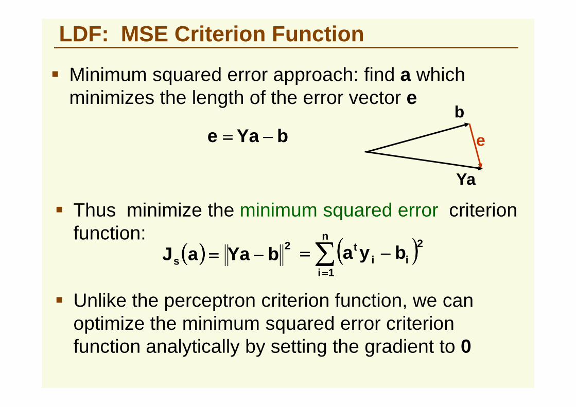
� Minimum squared error approach: find a which minimizes the length of the error vector e
bYae −−−−====
Ya
b
e
� Thus minimize the minimum squared error criterion � Thus minimize the minimum squared error criterion function:
(((( )))) 2bYaaJs −−−−====
� Unlike the perceptron criterion function, we can optimize the minimum squared error criterion function analytically by setting the gradient to 0
(((( ))))∑∑∑∑====
−−−−====n
iii
t bya1
2

LDF: Optimizing Js(a)
� Let’s compute the gradient:
(((( )))) 2bYaaJs −−−−==== (((( ))))∑∑∑∑
====
−−−−====n
iii
t bya1
2
(((( ))))
∂∂∂∂
∂∂∂∂∂∂∂∂
====∇∇∇∇
s
s
aJ
aJ M0
(((( ))))bYaY t −−−−==== 2(((( ))))
∂∂∂∂∂∂∂∂
====∇∇∇∇
d
s
s
aJ
aJ M (((( ))))bYaY −−−−==== 2
� Setting the gradient to 0:
(((( )))) bYYaYbYaY ttt ====⇒⇒⇒⇒====−−−− 02

LDF: Pseudo Inverse Solution
� Matrix YtY is square (it has d +1 rows and columns) and it is often non-singular
� If YtY is non-singular, its inverse exists and we can solve for a uniquely:
(((( )))) 1−−−−(((( )))) bYYYa tt 1−−−−====
pseudo inverse of Y
(((( ))))(((( )))) (((( )))) (((( )))) IYYYYYYYY tttt ========−−−−−−−− 11

LDF: Minimum Squared-Error Procedures
� If b1=…=bn =1, MSE procedure is equivalent to finding a hyperplane of best fit through the samples y1,…,yn
(((( )))) 2ns 1YaaJ −−−−====
nn
====
1
11 M
� Then we shift this line to the origin, if this line was a good fit, all samples will be classified correctly

LDF: Minimum Squared-Error Procedures
� Only guaranteed the separating hyperplane if Ya > 0
====
nt
1t
ya
yaYa M� that is if all elements of vector are positive
� That is where εεεε may be negative
++++
++++====
nnb
bYa
εεεε
εεεεM
11
� We have bYa ≈≈≈≈
� Thus in linearly separable case, least squares solution a does not necessarily gives separating hyperplane
� If εεεε1,…, εεεεn are small relative to b1,…, bn , then each element of Ya is positive, and a gives a separating hyperplane
++++ nnb εεεε
� If approximation is not good, εεεεi may be large and negative, for some i, thus bi + εεεεi will be negative and a is not a separating hyperplane
� But it will give a “reasonable” hyperplane

LDF: Minimum Squared-Error Procedures
� We are free to choose b. May be tempted to make blarge as a way to insure 0bYa >>>>≈≈≈≈
� Does not work� Let β β β β be a scalar, let’s try ββββb instead of b� if a* is a least squares solution to Ya = b, then for any
scalar ββββ, least squares solution to Ya = ββββb is ββββa*2
abYaminarg ββββ−−−− (((( )))) 22
ab/aYminarg −−−−==== ββββββββ
*aββββ====
� thus if for some i th element of Ya is less than 0, that is yt
ia < 0, then yti (ββββa) < 0,
� Relative difference between components of b matters, but not the size of each individual component
scalar ββββ, least squares solution to Ya = ββββb is ββββa*
(((( )))) 2
ab/aYminarg −−−−==== ββββ

LDF: Example
� Class 1: (6 9), (5 7)� Class 2: (5 9), (0 4)
� Set vectors y1, y2 , y3 , y4 by adding extra feature and “normalizing”
1 1 −−−−1 −−−−1
� Matrix Y is then
−−−−−−−−−−−−−−−−−−−−====
401951751961
Y
====
961
y1
====
751
y2
−−−−−−−−−−−−
====951
y3
−−−−
−−−−====
401
y 4

LDF: Example
� Choose
====
1111
b
� In matlab, a=Y\b solves the least squares problem
−−−−==== 0.1
7.2a
−−−−
====9.00.1a
� Note a is an approximation to Ya = b, since no exact solution exists
≠≠≠≠
====
1111
1.16.03.14.0
Ya
� This solution does give a separating hyperplane since Ya > 0
LDF: Example
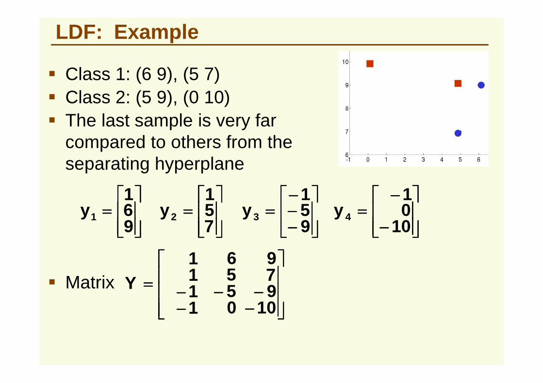
� Class 1: (6 9), (5 7)� Class 2: (5 9), (0 10)� The last sample is very far
compared to others from the separating hyperplane
1 1 −−−−1 −−−−1
� Matrix
−−−−−−−−−−−−−−−−−−−−====1001
951751961
Y
====
961
y1
====
751
y2
−−−−−−−−−−−−
====951
y3
−−−−
−−−−====
1001
y 4

LDF: Example
� Choose
====
1111
b
� In matlab, a=Y\b solves the least squares problem
−−−−==== 2.0
2.3a
−−−−
====4.02.0a
� Note a is an approximation to Ya = b, since no exact solution exists
≠≠≠≠
−−−−====1111
16.104.0
9.02.0
Ya
� This solution does not give a separating hyperplane since aty3 < 0

LDF: Example
� MSE pays to much attention to isolated “noisy” examples (such examples are called outliers)
outlierMSE solution
desired solution
� No problems with convergence though, and solution it gives ranges from reasonable to good

LDF: Example� we know that 4th point is far far
from separating hyperplane� In practice we don’t know this
� In Matlab, solve a=Y\b
====
10111
b� Thus appropriate
� In Matlab, solve a=Y\b
−−−−
−−−−====
9.07.11.1
a
� Note a is an approximation to Ya = b,
≠≠≠≠
====
10111
0.108.00.19.0
Ya
� This solution does give the separating hyperplane since Ya > 0

LDF: Gradient Descent for MSE solution
2. YtY may be close to singular if samples are highly correlated (rows of Y are almost linear combinations of each other)
� May wish to find MSE solution by gradient descent:
1. Computing the inverse of YtY may be too costly
(((( )))) 2bYaaJs −−−−====
combinations of each other)� computing the inverse of YtY is not numerically stable
� In the beginning of the lecture, computed the gradient:
(((( )))) (((( ))))bYaYaJ ts −−−−====∇∇∇∇ 2

LDF: Widrow-Hoff Procedure
� Thus the update rule for gradient descent:(((( )))) (((( )))) (((( )))) (((( ))))(((( ))))bYaYaa ktkkk −−−−−−−−====++++ ηηηη1
� If weight vector a(k) converges to the MSE solution a, that is Yt(Ya-b)=0
(((( )))) (((( )))) kk /1ηηηηηηηη ====
(((( )))) (((( ))))bYaYaJ ts −−−−====∇∇∇∇ 2
solution a, that is Yt(Ya-b)=0
� Widrow-Hoff procedure reduces storage requirements by considering single samples sequentially:
(((( )))) (((( )))) (((( )))) (((( ))))(((( ))))ikt
iikkk bayyaa −−−−−−−−====++++ ηηηη1

LDF: Ho-Kashyap Procedure
� Suppose training samples are linearly separable. Then there is as and positive bs s.t.
� In the MSE procedure, if b is chosen arbitrarily, finding separating hyperplane is not guaranteed
0>>>>==== ss bYa
� If we knew bs could apply MSE procedure to find the � If we knew bs could apply MSE procedure to find the separating hyperplane
� Idea: find both as and bs
� Minimize the following criterion function, restricting to positive b: (((( )))) 2
, bYabaJHK −−−−====

LDF: Ho-Kashyap Procedure
� As usual, take partial derivatives w.r.t. a and b
(((( )))) 2, bYabaJHK −−−−====
(((( )))) 02 ====−−−−====∇∇∇∇ bYaYJ tHKa
(((( )))) 02 ====−−−−−−−−====∇∇∇∇ bYaJHKb
� Use modified gradient descent procedure to find a � Use modified gradient descent procedure to find a minimum of JHK(a,b)
2) Fix a and minimize JHK(a,b) with respect to b
� Alternate the two steps below until convergence:1) Fix b and minimize JHK(a,b) with respect to a

LDF: Ho-Kashyap Procedure
(((( )))) 02 ====−−−−====∇∇∇∇ bYaYJ tHKa
(((( )))) 02 ====−−−−−−−−====∇∇∇∇ bYaJHKb
� Step (1) can be performed with pseudoinverse
2) Fix a and minimize JHK(a,b) with respect to b
� Alternate the two steps below until convergence:1) Fix b and minimize JHK(a,b) with respect to a
� For fixed b minimum of JHK(a,b) with respect to a is found by solving
(((( )))) 02 ====−−−− bYaY t
� Thus
(((( )))) bYYYa tt 1−−−−====

LDF: Ho-Kashyap Procedure
� We can’t use b = Ya because b has to be positive
� Step 2: fix a and minimize JHK(a,b) with respect to b
� Solution: use modified gradient descent
� start with positive b , follow negative gradient but refuse to decrease any components of b
� This can be achieved by setting all the positive components of to 0Jb∇∇∇∇
� Not doing steepest descent anymore, but we are still doing descent and ensure that b is positive

LDF: Ho-Kashyap Procedure� The Ho-Kashyap procedure:
0) Start with arbitrary a(1) and b(1) > 0, let k = 1
repeat steps (1) through (4)1) (((( )))) (((( )))) (((( ))))kkk bYae −−−−====
2) Solve for b(k+1) using a(k) and b(k)
(((( )))) (((( )))) (((( )))) (((( ))))[[[[ ]]]]||1 kkkk eebb ++++++++====++++ ηηηη
3) Solve for a(k+1) using b(k+1)
(((( )))) (((( )))) (((( ))))111 ++++−−−−++++ ==== kttk bYYYa
4) k = k + 1
until e(k) >= 0 or k > kmax or b(k+1) = b(k)
� For convergence, learning rate should be fixed between 0 < ηηηη < 1

LDF: Ho-Kashyap Procedure
� In the linearly separable case, � e(k) = 0, found solution, stop� one of components of e(k) is positive, algorithm continues
� In non separable case, � e(k) will have only negative components eventually, thus
found proof of nonseparability� No bound on how many iteration need for the proof of
nonseparability

LDF: Ho-Kashyap Procedure Example
� Class 1: (6 9), (5 7)� Class 1: (5 9), (0 10)
� Matrix
−−−−−−−−−−−−−−−−−−−−====1001
951751961
Y
1
� Use fixed learning ηηηη = 0.9
� Start with and (((( ))))
====
1111
b 1(((( ))))
====
111
a 1
� At the start (((( ))))
−−−−−−−−====
11151316
Ya 1

LDF: Ho-Kashyap Procedure Example
� solve for b(2) using a(1) and b(1)
� Iteration 1:
(((( )))) (((( )))) (((( ))))
−−−−
−−−−−−−−====−−−−====
1111
11151316
bYae 111�
−−−−−−−−====
12161215
(((( )))) (((( )))) (((( )))) (((( ))))[[[[ ]]]]|e|e9.0bb 1112 ++++++++====
++++
−−−−++++
==== 161215
161215
9.0111
==== 16.22
28
� solve for a(2) using b(2)
[[[[ ]]]]|e|e9.0bb ++++++++====
++++
−−−−−−−−++++
====1216
12169.0
11
====11
(((( )))) (((( )))) (((( )))) ====
−−−−−−−−−−−−−−−−−−−−
−−−−−−−−======== −−−−
116.22
28*
1.02.05.026.02.01.01.016.05.06.17.46.2
bYYYa 2t1t2
−−−− 8.37.26.34

LDF: Ho-Kashyap Procedure Example
� Continue iterations until Ya > 0� In practice, continue until minimum
component of Ya is less then 0.01
� After 104 iterations converged to solution
====
48.114.0
5.222.27
Ya
� a does gives a separating hyperplane
====
1471
2328
b
−−−−
−−−−====
3.113.279.34
a

m1,...,i )( 0 ====++++==== itii wxwxg
� Suppose we have m classes� Define m linear discriminant functions
� Given x, assign class ci if
ij )()( ≠≠≠≠∀∀∀∀≥≥≥≥ xgxg ji
LDF: MSE for Multiple Classes
ij )()( ≠≠≠≠∀∀∀∀≥≥≥≥ xgxg ji
� Such classifier is called a linear machine
� A linear machine divides the feature space into c decision regions, with gi(x) being the largest discriminant if x is in the region Ri

� For each class i, find weight vector ai, s.t.
LDF: MSE for Multiple Classes
∉∉∉∉∀∀∀∀====∈∈∈∈∀∀∀∀====
iclassy 0iclassy 1
yaya
ti
ti
� Let Yi be matrix whose rows are samples from class i, so it has d +1 columns and ni rowsclass i, so it has d +1 columns and ni rows
====
mY
YY
YM2
1
� Let’s pile all samples in n by d +1 matrix Y:
====
mclassfromsamplemclassfromsample
classfromsampleclassfromsample
M
11

� Let bi be a column vector of length n which is 0everywhere except rows corresponding to samples from class i, where it is 1:
LDF: MSE for Multiple Classes
====1
1
0
bi
M
M
M
rows corresponding to samples from class i
0M

LDF: MSE for Multiple Classes
[[[[ ]]]]n1 bbB L====
� Let’s pile all bi as columns in n by c matrix B
� Let’s pile all ai as columns in d +1 by m matrix A
[[[[ ]]]]maaA L1====
====
� m LSE problems can be represented in YA = B:
333211
classfromsampleclassfromsampleclassfromsampleclassfromsampleclassfromsampleclassfromsample
=
100100100010001001
Y A B

LDF: MSE for Multiple Classes
(((( )))) ∑∑∑∑====
−−−−====m
1i
2ii bYaAJ
� Our objective function is:
� J(A) is minimized with the use of pseudoinverse
(((( )))) YBYYA t 1−−−−====

LDF: Summary
� Perceptron procedures � find a separating hyperplane in the linearly separable case,� do not converge in the non-separable case� can force convergence by using a decreasing learning rate,
but are not guaranteed a reasonable stopping point
� MSE procedures � converge in separable and not separable case � converge in separable and not separable case � may not find separating hyperplane if classes are linearly
separable� use pseudoinverse if YtY is not singular and not too large� use gradient descent (Widrow-Hoff procedure) otherwise
� Ho-Kashyap procedures � always converge� find separating hyperplane in the linearly separable case� more costly
Recommended