Microfoundations of Financial Economics2004-2005
Professor André Farber
Solvay Business School
Université Libre de Bruxelles
PhD 03 |2April 18, 2023
CAPM: the real stuff
• Today we will look at various classical derivations of the CAPM.
• 1. Mossin
• Equilibrium of an exchange economy
• Based on quadratic utility functions
• 2. Mathematics of the efficient frontier
PhD 03 |3April 18, 2023
William Forsyth Sharpe
• From Wikipedia, the free encyclopedia.
• William Forsyth Sharpe (born June 16, 1934) is Professor of Finance, Emeritus at Stanford University's Graduate School of Business and the winner of the 1990 Bank of Sweden Prize in Economic Sciences in Memory of Alfred Nobel.
• Dr. Sharpe taught at the University of Washington and the University of California at Irvine. In 1970 he joined the Stanford University. He was one of the originators of the Capital Asset Pricing Model, created the Sharpe ratio for risk-adjusted investment performance analysis, contributed to the development of the binomial method for the valuation of options, the gradient method for asset allocation optimization, and returns-based style analysis for evaluating the style and performance of investment funds.
• He served as a President of the American Finance Association.
• He received his Ph.D., M.A., and B.A. in Economics from the University of California at Los Angeles. He is also the recipient of a Doctor of Humane Letters, Honoris Causa from DePaul University, a Doctor Honoris Causa from the University of Alicante (Spain), a Doctor Honoris Causa from the University of Vienna and the UCLA Medal, UCLA's highest honor.
– Bibliography
Portfolio Theory and Capital Markets (McGraw-Hill, 1970 and 2000)
Asset Allocation Tools (Scientific Press, 1987)
Fundamentals of Investments (with Gordon J. Alexander and Jeffrey Bailey, Prentice-Hall, 2000)
Investments (with Gordon J. Alexander and Jeffrey Bailey, Prentice-Hall, 1999)
PhD 03 |4April 18, 2023
John Lintner
• Wikipedia does not yet have a page called John Lintner.
To start the page, begin typing in the box below. When you're done, press the "Save page" button. Your changes should be visible immediately.
If you have created this page in the past few minutes and it has not yet appeared, it may not be visible due to a delay in updating the database. Please wait and check again later before attempting to recreate the page.
Please do not create an article to promote yourself, a website, a product, or a business (see Wikipedia:What Wikipedia is not).
If you are new to Wikipedia, please read the tutorial before creating your first article, and only use the sandbox for editing experiments.
Search for John Lintner in Wikipedia
PhD 03 |5April 18, 2023
Jan Mossin
• From Wikipedia, the free encyclopedia.
• Jan Mossin (b. 1936 in Oslo – d. 1987) was a Norwegian economist. He graduated with a siviløkonom degree from the Norwegian School of Economics and Business Administration (NHH) in 1959. After a couple of years in business, he started his PhD studies in the Spring semester of 1962 at Carnegie Mellon University (then Carnegie Institute of Technology).
• One of the papers in his doctoral dissertation was a very important contribution to the Capital Asset Pricing Model (CAPM). At Carnegie Mellon he was, among others, awarded the Alexander Henderson Award for 1968 for this contribution. If Jan Mossin had lived longer he would most likely had been a candidate for the Bank of Sweden Prize in Economic Sciences in Memory of Alfred Nobel in 1990 together with Professors Sharpe and Lintner.
• After he had finished his PhD he returned to NHH where he in 1968 was tenured professor.
PhD 03 |6April 18, 2023
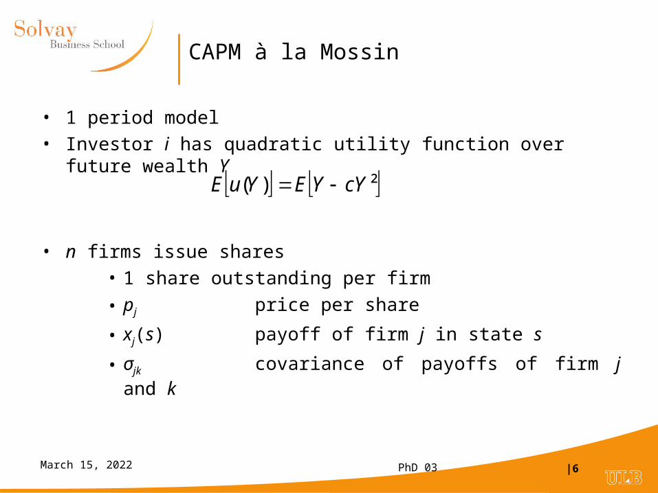
CAPM à la Mossin
• 1 period model
• Investor i has quadratic utility function over future wealth Y
• n firms issue shares
• 1 share outstanding per firm
• pj price per share
• xj(s) payoff of firm j in state s
• σjk covariance of payoffs of firm j and k
²)( cYYEYuE

PhD 03 |7April 18, 2023
Investor’s problem
ij
iii
z
cYYEYuE 2)(Max
j
jijii pzmW
jj
fjiji
f
jjiji
fi
pRxzWR
xzmRY
)(

PhD 03 |8April 18, 2023
FOC
njpRxYuEz
Uj
fji
ij
i ,...,1 0))(('
cYYu 21)('
k
if
ij
fjk
fkj
fjjkik WR
cpRxEpRxEpRxEz )
2
1)()(())()()((
)2
1(*
if
ijij WR
czz Note:
with zj* solution of:
k
jf
jkf
kjf
jjkk pRxEpRxEpRxEz ))(())()()((*
j=1,…,n
j=1,…,n

PhD 03 |9April 18, 2023
Market clearing conditions
i
ijz 1 j=1,…,n
0i
im
PhD 03 |10April 18, 2023
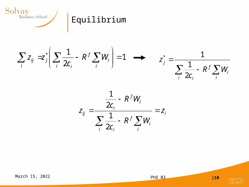
Equilibrium
12
1*
i ii
f
ij
iij WR
czz
i ii
f
i
j
WRc
z
2
11*
i
i ii
f
i
if
iij z
WRc
WRc
z
2
12
1
PhD 03 |11April 18, 2023
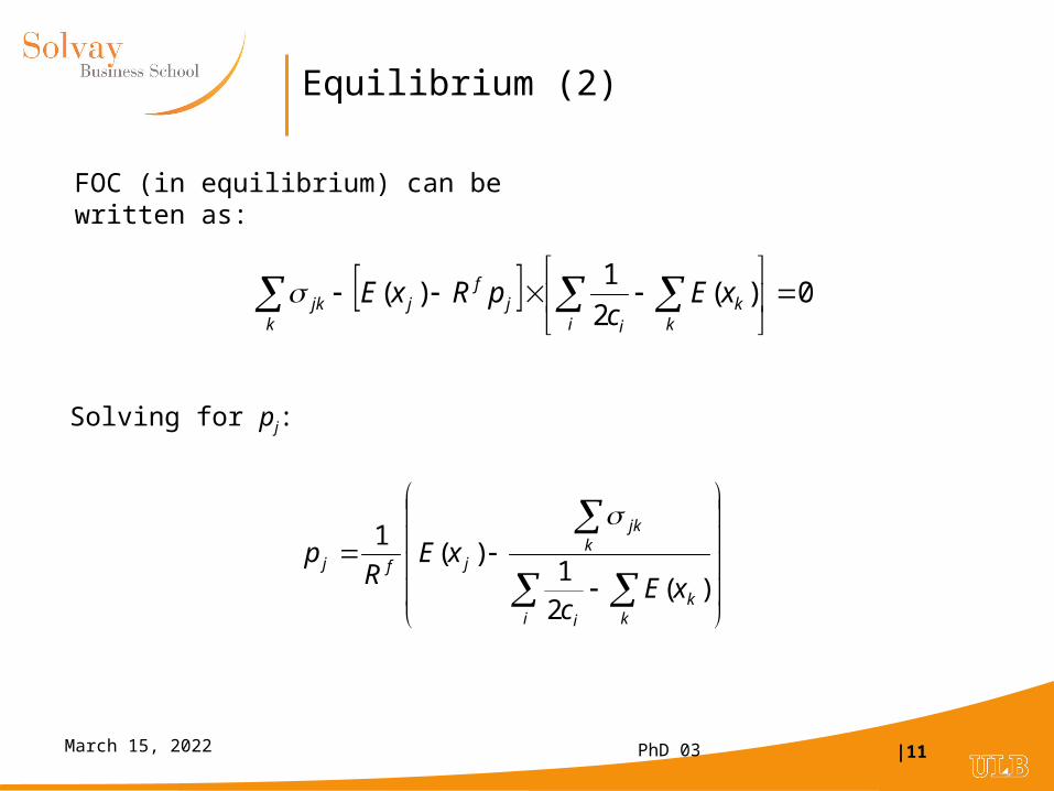
Equilibrium (2)
0)(2
1)(
k i kk
ij
fjjk xE
cpRxE
FOC (in equilibrium) can be written as:
i kk
i
kjk
jfj
xEc
xER
p)(
2
1)(
1
Solving for pj:
PhD 03 |12April 18, 2023
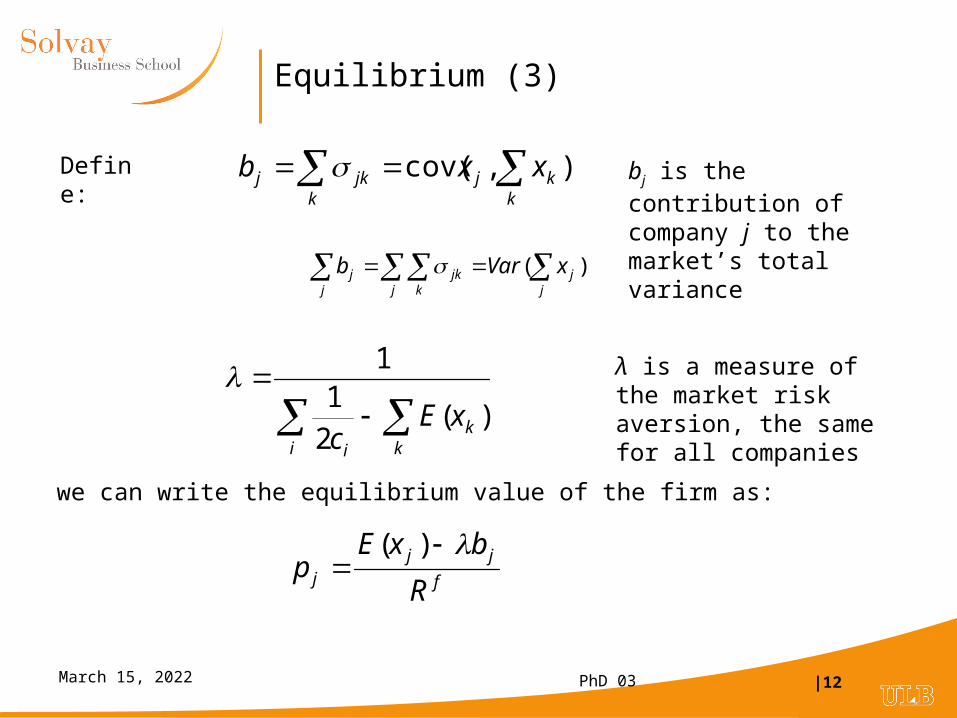
Equilibrium (3)
k
kjk
jkj xxb ),cov(
i kk
i
xEc
)(2
11
Define:
λ is a measure of the market risk aversion, the same for all companies
bj is the contribution of company j to the market’s total variance
j j k j
jjkj xVarb )(
we can write the equilibrium value of the firm as:
f
jjj R
bxEp
)(

PhD 03 |13April 18, 2023
Beta formulation
),cov()( MMMf
M RRpRRE
k
kM pp
The equilibrium price can be written as: k
kjjf
j xxxERp ),cov()(
Define:
j
jj p
xR
kkM xx
),cov(
),cov()(
MjMf
Mjf
j
RRpR
xRRRE
2
)(
M
fM
M
RREp
2
),cov()()(
M
MifM
fj
RRRRERRE

PhD 03 |14April 18, 2023
Mean-Variance Frontier Calculation: brute force
Mean variance portfolio: i j
ijjw
iw
Pn
wwwMin 2
,..,2
,1
jj
jjj
w
Eew
1
s.t.
Matrix notations:
w
VwwMin '
Eew '
1w’u=

PhD 03 |15April 18, 2023
Some math…
)'1(2)'(2'),,( 2121 uwewEVwwwL
01'
0'
021
wu
Ewe
ueVw
UEX 12
11
1''
''1
21
1
12
11
uVueVu
EuVeeVe
2111 ' ' ' ABCDuVuCeVeBuVeA
D
EABD
AEC
2
1
Ehgw
Lagrange:
FOC:
Define:
eVD
AuV
D
Bh
uVD
AeV
D
Cg
11
11
PhD 03 |16April 18, 2023
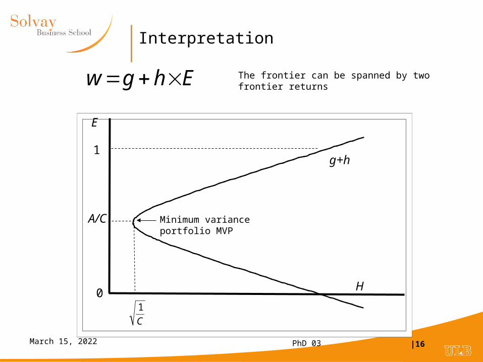
Interpretation
1g+h
0H
E
The frontier can be spanned by two frontier returns
Minimum variance portfolio MVPA/C
Ehgw
C
1
PhD 03 |17April 18, 2023
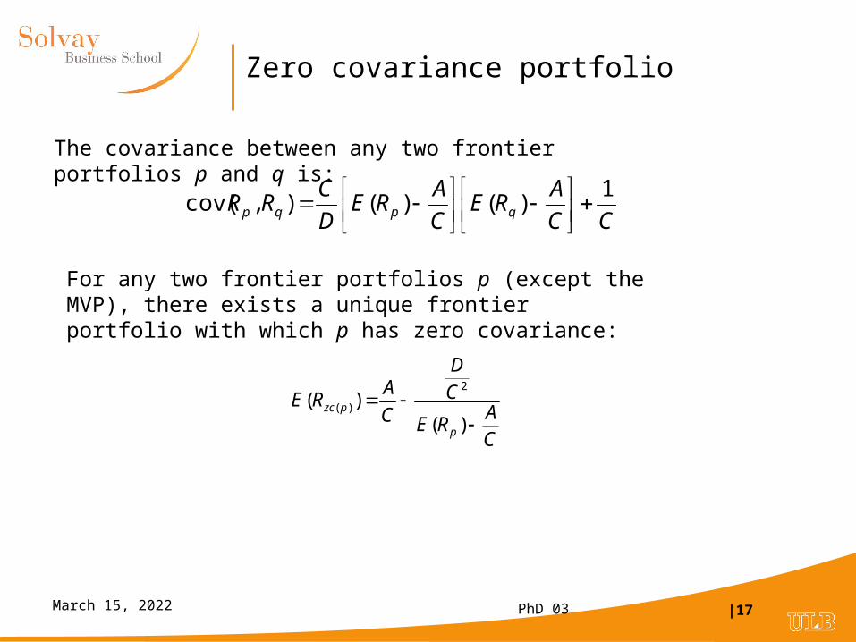
Zero covariance portfolio
CC
ARE
C
ARE
D
CRR qpqp
1)()(),cov(
The covariance between any two frontier portfolios p and q is:
For any two frontier portfolios p (except the MVP), there exists a unique frontier portfolio with which p has zero covariance:
CA
RE
CD
C
ARE
p
pzc
)()(
2
)(
PhD 03 |18April 18, 2023
0.800
0.900
1.000
1.100
1.200
1.300
1.400
0.000 0.050 0.100 0.150 0.200 0.250 0.300 0.350 0.400
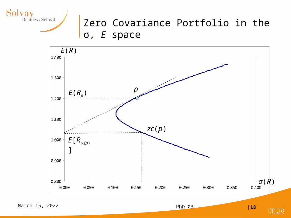
Zero Covariance Portfolio in the σ, E space
p
zc(p)
E[Rzc(p)]
E(Rp)
E(R)
σ(R)
PhD 03 |19April 18, 2023
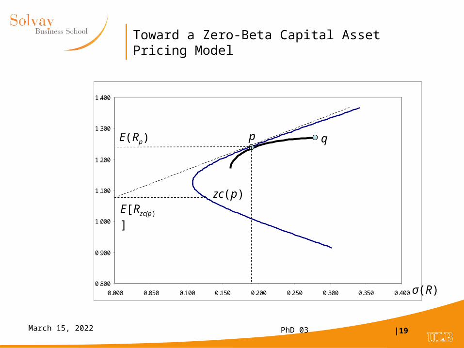
Toward a Zero-Beta Capital Asset Pricing Model
0.800
0.900
1.000
1.100
1.200
1.300
1.400
0.000 0.050 0.100 0.150 0.200 0.250 0.300 0.350 0.400
p q
zc(p)
E(Rp)
E[Rzc(p)]
σ(R)

PhD 03 |20April 18, 2023
Some math
)(),cov( qqp RERR
)(0 )( pzcRE
)()(),cov( )( pzcqqp RERERR
)()(),cov( )(2
pzcpppp RERERR
)()(
)()(),cov(
)(
)(
2pzcp
pzcq
p
qp
RERE
RERERR
Proof on demand – see DD Chap 7
Apply to ZC portfolio:
Apply to p:
Divide:
Rearrange: )()()()( )()( pzcpqppzcq RERERERE

PhD 03 |21April 18, 2023
Another proof (more intuitive??)
0)(
)(
aP
P
Rd
RdE
)(
)()( )(
p
pzcp
R
RERE
)(2))(),(cov(2
1)()(
)(
)(
)(
)(
)(
)(
0
2
2
0
ppqp
pq
aP
p
p
p
aP
P
RRRR
RERE
Rd
Rd
Rd
da
da
RdE
Rd
RdE
Consider a fraction a invested in stock q and (1-a) in p
The slope
is equal to the slope of tangent
As:
)()()()( )()( pzcpqppzcq RERERERE

PhD 03 |22April 18, 2023
Zero-Beta CAPM
)()()()( )()( MzcMjMMzcj RERERERE
In equilibrium, the market portfolio is on the efficient frontier
If there exist a risk free asset: E(Rzc(M)) = Rf
Empirical test: Roll critique
If proxy used for the market portfolio, linear relationship doesn’t hold
PhD 03 |23April 18, 2023
Next session
• Efficient frontier in Hilbert space (wooow..)
• Where are the SDF in the CAPM?
Recommended