Measuring Ground Deformation usingOptical Imagery
Sebastien Leprince
California Institute of Technology, USA
October 29, 2009Keck Institute for Space Studies Workshop

Measuring Horizontal Ground Displacement,Methodology Flow
Inputs:
Raw images
Orbits, platform attitudes,
camera model
Digital Elevation Model
Orthorectification:
Images must superimpose accurately
Correlation:
Outputs:
N/S offset field E/W offset field SNR
Displacement
in rows and
columns
provide the
E/W and N/S
components of
the ground
deformation
The Signal to
Noise Ratio
assesses the
measure
quality.
Pre-earthquake i
mage
Post-earthquake i
mageSub-pixel
Correlation

Orthorectification ModelPushbroom acquisition geometry
look direction of pixel (c, r)
satellite velocity
CCD array
absolute pointing error from ancillary
data
CCD acquiring column c
PSat = O
M
▶ O, optical center in space
▶ M, ground point seen bypixel p
▶ u1 pixel pointing model
▶ R(p) 3D rotation matrix, roll,pitch, yaw at p
▶ T(p) Terrestrial coordinatesconversion
▶ δ correction on the lookdirections to insurecoregistration
▶ λ > 0
M(p) = O(p) + λ[T(p)R(p)u1(p) + δ(p)
]

Image Correlation: local rigid translations
▶ Fourier Shift Theorem
i2(x, y) = i1(x− ∆x, y− ∆y)
I2(ωx, ωy) = I1(ωx, ωy)e−j(ωx∆x+ωy∆y)
▶ Normalized Cross-spectrum
Ci1i2 (ωx, ωy) =I1(ωx, ωy)I∗2 (ωx, ωy)
∣I1(ωx, ωy)I∗2 (ωx, ωy)∣= ej(ωx∆x+ωy∆y)
▶ Finding the relative displacement
φ(∆x, ∆y) =π
∑ωx=−π
π
∑ωy=−π
W(ωx, ωy)∣Ci1i2 (ωx, ωy)− ej(ωx∆x+ωy∆y)∣2
W weighting matrix. (∆x, ∆y) such that φ minimum.
S. Leprince et al., IEEE TGRS, 2007

Processing Chain
Select Image
Registration Patches
from raw image
Orthorectify patches
Resample
image patches
Correlate patches,
find relative displacement
with reference
Deduce viewing
correction δ
for co-registration
Orthorectify / resample
image 2
Orthorectify / resample
image 1
Correlation on sliding
windows
Horizontal deformation
map
S. Leprince et al., IEEE TGRS, 2007

1999 Mw 7.1 Hector Mine Earthquake, CA

1999 Mw 7.1 Hector Mine Earthquake, CA

1999 Mw 7.1 Hector Mine Earthquake, CA
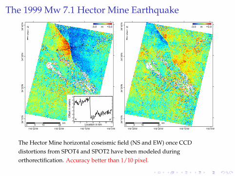
The 1999 Mw 7.1 Hector Mine Earthquake
-3.0 m +3.0
³
0 10 205km
116°30'W 116°20'W 116°10'W 116°0'W
34°10'N
34°20'N
34°30'N
34°40'N
0 2 4 6 8 10 12
-4
-3
-2
-1
0
1
2
3
Location in km
Offset in
mete
rs
A A'
A
A'
-3.0 m +3.0
³
0 10 205km
116°30'W 116°20'W 116°10'W 116°0'W
34°10'N
34°20'N
34°30'N
34°40'N
The Hector Mine horizontal coseismic field (NS and EW) once CCDdistortions from SPOT4 and SPOT2 have been modeled duringorthorectification. Accuracy better than 1/10 pixel.

The Mer de Glace Glacier, France6°54'0"E 6°56'0"E 6°58'0"E
45°5
2'0
"N45°5
4'0
"N45°5
6'0
"N
2000 m
³
26 days horizontal
displacement (m)0 5 10 15 20 25 30 35 40 45 50 55
A
A'
B
B'
-800 -600 -400 -200 0 200 400 600 800
0
4
8
12
16
20
Transversal distance (meters)
A A'
B B'
Dis
pla
ce
me
nt
ove
r 2
6 d
ays (
m)
0 2 4 6 8 10 12 14 16 18 200
1
2
3
4
5
6
Dis
tan
ce
(km
) a
lon
g N
ort
h d
ire
ctio
n
12.5m
longitudinal
average
Raw correlation
measurements
GPS
measurements
Displacement in meters over 26 days
(a) (b)
(c)
Mer de
Glace Talèfre
Leschaux
B - B'
A - A'
S. Leprince, et al., EOS, 2008
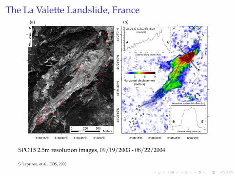
The La Valette Landslide, France
6°39'0"E6°38'45"E6°38'30"E6°38'15"E
0 250 500Meters
³
6°39'0"E6°38'45"E6°38'30"E6°38'15"E
44
°25
'0"N
44
°24
'45
"N4
4°2
4'3
0"N
44
°24
'15
"N
A'
A
B'
B
1
2
3
4
5
6
7
8
9
0 0.2 0.4 0.6 0.8 1 1.2 1.4 1.60
Distance along profile (Km)
Absolute horizontal offset(meters)
A A'
-50 0 500
1
2
3
4
5
6
7
Distance along profile (m)
Absolute horizontal offset (m)
B B'
Horizontal displacement
(meters)
0 3 6 9
(a) (b)
SPOT5 2.5m resolution images, 09/19/2003 - 08/22/2004
S. Leprince, et al., EOS, 2008

Geometrical Distortions: CCD misalignement
116°30'W 116°20'W 116°10'W 116°0'W
34
°10
'N3
4°2
0'N
34
°30
'N3
4°4
0'N
0 10 205km
³-3.0 m +3.0
Interconnection
inaccuracies of
the linear CCD
arrays of the
sensor
Secondary
branch of
the rupture
A
A'
0 2 4 6 8 10 12-4
-3
-2
-1
0
1
2
3
Location in km
Offset in
mete
rs
A A'
116°30'W 116°20'W 116°10'W 116°0'W
34
°10
'N3
4°2
0'N
34
°30
'N3
4°4
0'N
0 10 205km
³-3.0 m +3.0
CCD
artifact
Topography
artifacts
generated
from the
CCD array
distortions
The Hector Mine horizontal coseismic field (NS and EW) showing linearartifacts due to CCD misalignment. The geometry of the CCD sensor has tobe well modeled.
S. Leprince et al., IEEE TGRS, 2008

Geometrical Distortions: CCD misalignement
SPOT CCD distortions
-0.1
0
0.1 Across-track (X) distortion in pixelinter-array
discontinuity
1500 3000 4500 6000
-0.1
0
0.1
CCD number:
Along-track (Y) distortion in pixel
▶ CCD Calibration model (1/100 pixel accurate) for SPOT 4-HRV1
S. Leprince et al., IEEE TGRS, 2008

ASTER attitude variations: The 2005 Mw 7.6 Kashmir Earthquake
73°10'E 73°20'E 73°30'E 73°40'E 73°50'E
34°1
0'N
34°2
0'N
34°3
0'N
³0 10 205 Km
-10 -5 0 5 10 15
Northward offset (m)
-15
10 5 0
-5
10 5 0
-5
Un-
reco
rded
pitc
h va
riatio
ns fr
om T
erra
sat
ellit
e(m
eter
s)
15
Faultrupture
Along-track
direction
Northward component of the correlation from 15m ASTER images acquiredon 11/14/2000 and 10/27/2005. Before, and after removing pitch artifacts(destripping). Deformation mostly perpendicular to the fault that could notbe measured on the field
Leprince et al., IGARSS 2007 / Avouac et al., EPSL, 2006

Topography error: modeling
Scherler et al., RSE 2008
D = h(tan(θ1)− tan(θ2))
▶ The measurement error Dresults from a trade-offbetween a well resolvedtopography and incidenceangles difference.
▶ D lives in the plane (p1Mp2),called the epipolar plane.For pushbroom systems, thisplane is generally in theacross-track direction, henceEW components are usuallyaffected the most by topobiases.

Aliasing effects in deformation maps: 2001 Bhuj earthquake
using SPOT images▶ Optical images often
aliased (CCD do notproperly sampleinstrument PSF)
▶ Aliasing effects producewhite noise whenacquisitions havedifferent viewinggeometry
▶ Aliasing strongly biassubpixel measurementwhen images havesimilar viewinggeometry
▶ Image de-aliasing orsingle imagesuper-resolution still anopen problem and areaof active research

Future challenge for large scale monitoring
▶ Thus far:
▶ Semi-automatic processing: manual selection of registrationpoints. Sufficient for studies with a few dozen of images
▶ Only a handful of registration points is necessary per image
▶ The key to large scale processing:▶ Automatic determination of a few “robust” registration
points per image
▶ Techniques such as SIFT can be useful to achieve this goal▶ Tricky problem when dealing with ground displacement,
because registration points should be selected on stableground

Conclusion:
▶ The technique has broad applications and is valuable to measure manydifferent surface processes, e.g, glacier flow, landslides, sand dunesmigration, volcanoes
▶ Generally valuable to any change detection application, wheneverprecise co-registration of images and/or spectral bands is required(vegetation, agriculture, land monitoring, etc...)
▶ Could envision operational high resolution global monitoring of Earthsurface changes using current satellite image databases for, e.g, largescale monitoring of mountainous glaciers, desertification, deforestation,etc...
▶ Optical imaging satellites have not been designed for measuringground deformation. New applications might put new constraints onthe design of future missions (tighter geometric constraints, higherimage sampling, etc...)

The End: Thank you!
Questions?
COSI-Corrweb site
http://www.tectonics.caltech.edu/slip history/spot coseis/
Recommended