Mathematical methods for Image Processing
Francois Malgouyres
Institut de Mathematiques de Toulouse, France
invitation byJidesh P., NITK Surathkal
fundingGlobal Initiative on Academic Network
Oct. 23–27
Francois Malgouyres (IMT) Mathematics for Image Processing Oct. 23–27 1 / 26

Plan
1 Introduction to image processing and mathematical optimization
Francois Malgouyres (IMT) Mathematics for Image Processing Oct. 23–27 2 / 26

Introduction to image processing
Applications:
◮ Pictures and movies◮ medical imaging (CT, TEP, MRI. . . )◮ Biological image (microscopy)◮ Earth observation (security, climat. . . )◮ Surveillance, safety (problem detection. . . )◮ Astronomy, astrophysics
Tools:
◮ Compression◮ Restoration◮ Segmentation◮ Registration◮ Indexation◮ Editing
Francois Malgouyres (IMT) Mathematics for Image Processing Oct. 23–27 3 / 26
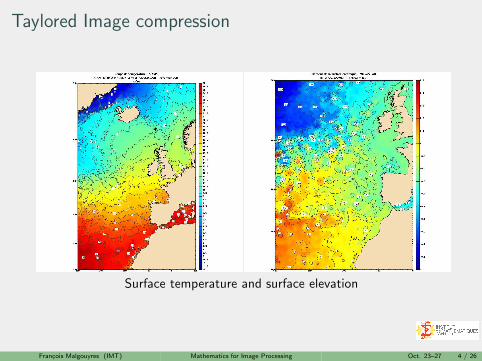
Taylored Image compression
Surface temperature and surface elevation
Francois Malgouyres (IMT) Mathematics for Image Processing Oct. 23–27 4 / 26
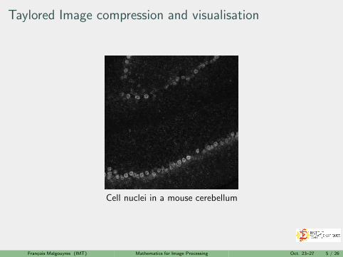
Taylored Image compression and visualisation
Cell nuclei in a mouse cerebellum
Francois Malgouyres (IMT) Mathematics for Image Processing Oct. 23–27 5 / 26
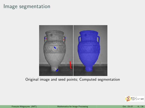
Image segmentation
Original image and seed points; Computed segmentation
Francois Malgouyres (IMT) Mathematics for Image Processing Oct. 23–27 6 / 26

Image segmentation
Segmentation of a lung tumor
Francois Malgouyres (IMT) Mathematics for Image Processing Oct. 23–27 7 / 26
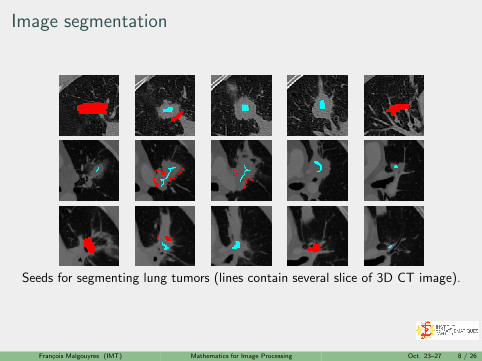
Image segmentation
Seeds for segmenting lung tumors (lines contain several slice of 3D CT image).
Francois Malgouyres (IMT) Mathematics for Image Processing Oct. 23–27 8 / 26

Image segmentation
Segmentation: Correct (yellow), expert only (red), system only (blue)
Francois Malgouyres (IMT) Mathematics for Image Processing Oct. 23–27 9 / 26

Image registration
Registration of consecutive images in a movie
Francois Malgouyres (IMT) Mathematics for Image Processing Oct. 23–27 10 / 26

Image restoration : denoising
Top: noisy images; Bottom: denoised images .
Francois Malgouyres (IMT) Mathematics for Image Processing Oct. 23–27 11 / 26

Image restoration : deblurring
Top: blurred image; Bottom: restored and ideal image.
Francois Malgouyres (IMT) Mathematics for Image Processing Oct. 23–27 12 / 26

Image restoration : inpainting
Top: Image with missing pixels; Bottom: restored and ideal image
Francois Malgouyres (IMT) Mathematics for Image Processing Oct. 23–27 13 / 26
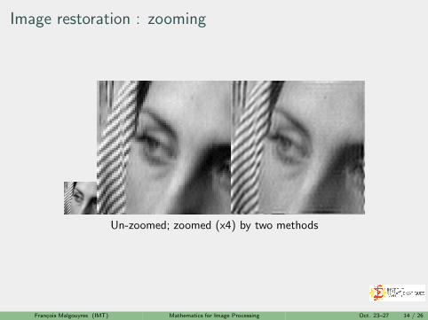
Image restoration : zooming
Un-zoomed; zoomed (x4) by two methods
Francois Malgouyres (IMT) Mathematics for Image Processing Oct. 23–27 14 / 26

Restoration of compressed images
Top: compressed images (for differents compression level). Bottom: restoredimages
Francois Malgouyres (IMT) Mathematics for Image Processing Oct. 23–27 15 / 26
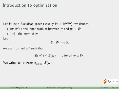
Introduction to optimization
Let W be a Euclidean space (usually W = RN×N), we denote
〈w ,w ′〉 : the inner product between w and w ′ ∈ W
‖w‖: the norm of w
LetE : W −→ R
we want to find w∗ such that
E (w∗) ≤ E (w) , for all w ∈ W .
We write: w∗ ∈ Argminw∈W
E (w).
Francois Malgouyres (IMT) Mathematics for Image Processing Oct. 23–27 16 / 26

Introduction to optimization: Examples
Below ∇ is a finite difference operator and T is a ”sparsifying transform”
H1 regularization
E (w) =
N−1∑
m,n=0
|∇wm,n|2 + λ‖w − u‖2
Total variation regularization
E (w) =
N−1∑
m,n=0
|∇wm,n|+ λ‖w − u‖2
ℓ1 minimisationE (w) = ‖w‖1 + λ‖Tw − u‖2
Francois Malgouyres (IMT) Mathematics for Image Processing Oct. 23–27 17 / 26

Introduction to optimization
The design ofE : W −→ R
is crucial. We want:
Guarantee that w∗ is close to the targeted ideal image◮ statistics, compressed sensing
Francois Malgouyres (IMT) Mathematics for Image Processing Oct. 23–27 18 / 26

Introduction to optimization
The design ofE : W −→ R
is crucial. We want:
Guarantee that w∗ is close to the targeted ideal image◮ statistics, compressed sensing
w∗ exists and can be numericaly approximated in a reasonable amount oftime
◮ Mathematical optimization
Francois Malgouyres (IMT) Mathematics for Image Processing Oct. 23–27 18 / 26

Introduction to optimization: basic properties of functions
Definition
Let E : W −→ R
E is proper iif◮ ∀w ∈ W, we have E(w) > −∞
◮ there exists w ∈ W such that E(w) < +∞
E is lower-semicontinuous iif ∀w ∈ W , ∀ε > 0 there is a neighborhood ofw such that ∀w ′ ∈ U ,E (w ′) ≥ E (w)− ε
E is coercive iif lim‖w‖→+∞ E (w) = +∞
Francois Malgouyres (IMT) Mathematics for Image Processing Oct. 23–27 19 / 26

Introduction to optimization: basic properties of functions
Definition
Let t ∈ R, we call t-levelset of E :
LE (t) = {w ∈ W |E (w) ≤ t}
Proposition
Let E : W −→ R
If E is proper, lower-semicontinuous and coercive, then
for every t ∈ R,LE (t) is compact
If E is proper, lower-semicontinuous and coercive then
Argminw∈W E (w) 6= ∅.
Francois Malgouyres (IMT) Mathematics for Image Processing Oct. 23–27 20 / 26
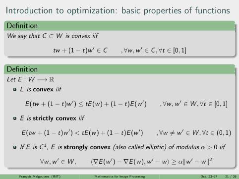
Introduction to optimization: basic properties of functions
Definition
We say that C ⊂ W is convex iif
tw + (1− t)w ′ ∈ C , ∀w ,w ′ ∈ C , ∀t ∈ [0, 1]
Definition
Let E : W −→ R
E is convex iif
E (tw + (1 − t)w ′) ≤ tE (w) + (1− t)E (w ′) , ∀w ,w ′ ∈ W , ∀t ∈ [0, 1]
E is strictly convex iif
E (tw + (1− t)w ′) < tE (w) + (1− t)E (w ′) , ∀w 6= w ′ ∈ W , ∀t ∈ (0, 1)
If E is C 1, E is strongly convex (also called elliptic) of modulus α > 0 iif
∀w ,w ′ ∈ W , 〈∇E (w ′)−∇E (w),w ′ − w〉 ≥ α‖w ′ − w‖2
Francois Malgouyres (IMT) Mathematics for Image Processing Oct. 23–27 21 / 26
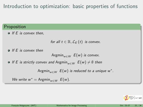
Introduction to optimization: basic properties of functions
Proposition
If E is convex then,
for all t ∈ R,LE (t) is convex.
If E is convex thenArgminw∈W E (w) is convex.
If E is strictly convex and Argminw∈W
E (w) 6= ∅ then
Argminw∈W E (w) is reduced to a unique w∗.
We write w∗ = Argminw∈W E (w).
Francois Malgouyres (IMT) Mathematics for Image Processing Oct. 23–27 22 / 26
Introduction to optimization: basic properties of functions
Proposition
If E is convex, then E is continuous on the interior of
Dom(E ) = {w ∈ W |E (w) < +∞}.
Proposition
If E is C 1,
E is convex iif
∀w ,w ′ ∈ W , E (w ′) ≥ E (w) + 〈∇E (w),w ′ − w〉
E is strongly convex of modulus α > 0 iif
∀w ,w ′ ∈ W , E (w ′) ≥ E (w) + 〈∇E (w),w ′ − w〉+α
2‖w ′ − w‖2
If E is strongly convex then E is strictly convex and coercive.
Francois Malgouyres (IMT) Mathematics for Image Processing Oct. 23–27 23 / 26
Introduction to optimization: basic properties of functions
Definition
Let E be convex. For any w ∈ W we call sub-gradient of E at w
∂E (w) = {g ∈ W |∀w ′ ∈ W ,E (w ′) ≥ E (w) + 〈g ,w ′ − w〉}
Proposition
Let E be convex.
If E is C 1 then∂E (w) = {∇E (w)}.
w∗ ∈ Argminw∈W E (w) iif 0 ∈ ∂E (w∗).
Francois Malgouyres (IMT) Mathematics for Image Processing Oct. 23–27 24 / 26

Introduction to optimization: basic properties of functions
Definition
Let L > 0, we say that E has Lipschitz gradient of parameter L iif
∀w ,w ′ ∈ W , ‖∇E (w ′)−∇E (w)‖ ≤ L‖w ′ − w‖
Proposition
If E is C 2 (its Hessian is denoted ∇2E (w)):
E is strongly convex of modulus α > 0 iif the smallest eigenvalue of ∇2E (w)is larger than α, for all w ∈ W.
E has a L-Lipschitz gradient iif the largest eigenvalue of ∇2E (w) is smallerthan L, for all w ∈ W.
Francois Malgouyres (IMT) Mathematics for Image Processing Oct. 23–27 25 / 26
Introduction to optimization: To go further
”Introductory lectures on convex optimization: A basic course”, YuriiNesterov
”Convex Analysis”, Ralph T. Rockafellar
”Non linear programming”, Dimitri Bertzekas
Francois Malgouyres (IMT) Mathematics for Image Processing Oct. 23–27 26 / 26
Recommended