(more info)

Math for the people, by the people. Encyclopedia | Requests | Forums | Docs | Wiki | Random | RSS

Advanced search

topological space (Definition)

"topological space" is owned by djao. [ full author list (2) ]

(more info)

Math for the people, by the people. Encyclopedia | Requests | Forums | Docs | Wiki | Random | RSS

Advanced search

compact (Definition)

"compact" is owned by djao. [ full author list (2) ]

Dense set 1

Dense setIn topology and related areas of mathematics, a subset A of a topological space X is called dense (in X) if any point xin X belongs to A or is a limit point of A.[1] Informally, for every point in X, the point is either in A or arbitrarily"close" to a member of A - for instance, every real number is either a rational number or has one arbitrarily close to it(see Diophantine approximation).Formally, a subset A of a topological space X is dense in X if for any point x in X, any neighborhood of x contains atleast one point from A. Equivalently, A is dense in X if and only if the only closed subset of X containing A is Xitself. This can also be expressed by saying that the closure of A is X, or that the interior of the complement of A isempty.The density of a topological space X is the least cardinality of a dense subset of X.

Density in metric spacesAn alternative definition of dense set in the case of metric spaces is the following. When the topology of X is givenby a metric, the closure of A in X is the union of A and the set of all limits of sequences of elements in A (its limitpoints),

Then A is dense in X if

Note that . If is a sequence of dense open sets in a complete metric

space, X, then is also dense in X. This fact is one of the equivalent forms of the Baire category theorem.

ExamplesThe real numbers with the usual topology have the rational numbers as a countable dense subset which shows thatthe cardinality of a dense subset of a topological space may be strictly smaller than the cardinality of the space itself.The irrational numbers are another dense subset which shows that a topological space may have several disjointdense subsets.By the Weierstrass approximation theorem, any given complex-valued continuous function defined on a closedinterval [a,b] can be uniformly approximated as closely as desired by a polynomial function. In other words, thepolynomial functions are dense in the space C[a,b] of continuous complex-valued functions on the interval [a,b],equipped with the supremum norm.Every metric space is dense in its completion.

PropertiesEvery topological space is dense in itself. For a set X equipped with the discrete topology the whole space is the onlydense set. Every non-empty subset of a set X equipped with the trivial topology is dense, and every topology forwhich every non-empty subset is dense must be trivial.Denseness is transitive: Given three subsets A, B and C of a topological space X with A ⊆ B ⊆ C such that A is densein B and B is dense in C (in the respective subspace topology) then A is also dense in C.The image of a dense subset under a surjective continuous function is again dense. The density of a topological spaceis a topological invariant.A topological space with a connected dense subset is necessarily connected itself.

Dense set 2

Continuous functions into Hausdorff spaces are determined by their values on dense subsets: if two continuousfunctions f, g : X → Y into a Hausdorff space Y agree on a dense subset of X then they agree on all of X.

Related notionsA point x of a subset A of a topological space X is called a limit point of A (in X) if every neighbourhood of x alsocontains a point of A other than x itself, and an isolated point of A otherwise. A subset without isolated points is saidto be dense-in-itself.A subset A of a topological space X is called nowhere dense (in X) if there is no neighborhood in X on which A isdense. Equivalently, a subset of a topological space is nowhere dense if and only if the interior of its closure isempty. The interior of the complement of a nowhere dense set is always dense. The complement of a closed nowheredense set is a dense open set.A topological space with a countable dense subset is called separable. A topological space is a Baire space if andonly if the intersection of countably many dense open sets is always dense. A topological space is called resolvable ifit is the union of two disjoint dense subsets. More generally, a topological space is called κ-resolvable if it contains κpairwise disjoint dense sets.An embedding of a topological space X as a dense subset of a compact space is called a compactification of X.A linear operator between topological vector spaces X and Y is said to be densely defined if its domain is a densesubset of X and if its range is contained within Y. See also continuous linear extension.A topological space X is hyperconnected if and only if every nonempty open set is dense in X. A topological space issubmaximal if and only if every dense subset is open.

References

Notes[1] Steen, L. A.; Seebach, J. A. (1995), Counterexamples in Topology, Dover, ISBN 048668735X

General references• Nicolas Bourbaki (1989) [1971]. General Topology, Chapters 1–4. Elements of Mathematics. Springer-Verlag.

ISBN 3-540-64241-2.• Steen, Lynn Arthur; Seebach, J. Arthur Jr. (1995) [1978], Counterexamples in Topology (Dover reprint of 1978

ed.), Berlin, New York: Springer-Verlag, ISBN 978-0-486-68735-3, MR507446

Article Sources and Contributors 3

Article Sources and ContributorsDense set  Source: http://en.wikipedia.org/w/index.php?oldid=456661398  Contributors: A19grey, Aleph4, Archelon, Austinmohr, Banus, Bdmy, Bluestarlight37, Calle, Can't sleep, clown willeat me, CiaPan, Cuaxdon, Denis.arnaud, Dino, ELLusKa 86, Erzbischof, Fly by Night, Giftlite, Graham87, Haemo, Headbomb, Isnow, Kae1is, Macrakis, Maksim-e, MathMartin, Michael Hardy,Mks004, Nguyen Thanh Quang, Oleg Alexandrov, Physicistjedi, Poulpy, Tobias Bergemann, Utkwes, Vundicind, 25 ,דניאל ב., דניאל צבי anonymous edits

LicenseCreative Commons Attribution-Share Alike 3.0 Unported//creativecommons.org/licenses/by-sa/3.0/

Homeomorphism 1

Homeomorphism

A continuous deformation between a coffee mugand a donut illustrating that they are

homeomorphic. But there need not be acontinuous deformation for two spaces to be

homeomorphic—only a continuous mapping witha continuous inverse.

In the mathematical field of topology, a homeomorphism ortopological isomorphism or bicontinuous function is a continuousfunction between topological spaces that has a continuous inversefunction. Homeomorphisms are the isomorphisms in the category oftopological spaces—that is, they are the mappings that preserve all thetopological properties of a given space. Two spaces with ahomeomorphism between them are called homeomorphic, and from atopological viewpoint they are the same.

Roughly speaking, a topological space is a geometric object, and thehomeomorphism is a continuous stretching and bending of the objectinto a new shape. Thus, a square and a circle are homeomorphic toeach other, but a sphere and a donut are not. An often-repeatedmathematical joke is that topologists can't tell their coffee cup fromtheir donut,[1] since a sufficiently pliable donut could be reshaped tothe form of a coffee cup by creating a dimple and progressivelyenlarging it, while shrinking the hole into a handle.

Topology is the study of those properties of objects that do not changewhen homeomorphisms are applied. As Henri Poincaré famously said, mathematics is not the study of objects, butinstead, the relations (isomorphisms for instance) between them.

DefinitionA function f: X → Y between two topological spaces (X, TX) and (Y, TY) is called a homeomorphism if it has thefollowing properties:• f is a bijection (one-to-one and onto),• f is continuous,• the inverse function f −1 is continuous (f is an open mapping).A function with these three properties is sometimes called bicontinuous. If such a function exists, we say X and Yare homeomorphic. A self-homeomorphism is a homeomorphism of a topological space and itself. Thehomeomorphisms form an equivalence relation on the class of all topological spaces. The resulting equivalenceclasses are called homeomorphism classes.

Homeomorphism 2

Examples

A trefoil knot is homeomorphic to a circle.Continuous mappings are not always realizable asdeformations. Here the knot has been thickened

to make the image understandable.

• The unit 2-disc D2 and the unit square in R2 are homeomorphic.• The open interval (a, b) is homeomorphic to the real numbers R for

any a < b.• The product space S1 × S1 and the two-dimensional torus are

homeomorphic.• Every uniform isomorphism and isometric isomorphism is a

homeomorphism.• Any 2-sphere with a single point removed is homeomorphic to the

set of all points in R2 (a 2-dimensional plane). (Here we use2-sphere in the sense of a physical beach ball, not a circle or 4-ball.)

• Let A be a commutative ring with unity and let S be a multiplicativesubset of A. Then Spec(AS) is homeomorphic to {p ∈ Spec(A) : p ∩S = ∅}.

• Rm and Rn are not homeomorphic for m ≠ n.• The Euclidean real line is not homeomorphic to the unit circle as a subspace of R2 as the unit circle is compact as

a subspace of Euclidean R2 but the real line is not compact.

NotesThe third requirement, that f −1 be continuous, is essential. Consider for instance the function f: [0, 2π) → S1 definedby f(φ) = (cos(φ), sin(φ)). This function is bijective and continuous, but not a homeomorphism (S1 is compact but [0,2π) is not).Homeomorphisms are the isomorphisms in the category of topological spaces. As such, the composition of twohomeomorphisms is again a homeomorphism, and the set of all self-homeomorphisms X → X forms a group, calledthe homeomorphism group of X, often denoted Homeo(X); this group can be given a topology, such as thecompact-open topology, making it a topological group.For some purposes, the homeomorphism group happens to be too big, but by means of the isotopy relation, one canreduce this group to the mapping class group.Similarly, as usual in category theory, given two spaces that are homeomorphic, the space of homeomorphismsbetween them, Homeo(X, Y), is a torsor for the homeomorphism groups Homeo(X) and Homeo(Y), and given aspecific homeomorphism between X and Y, all three sets are identified.

Properties• Two homeomorphic spaces share the same topological properties. For example, if one of them is compact, then

the other is as well; if one of them is connected, then the other is as well; if one of them is Hausdorff, then theother is as well; their homotopy & homology groups will coincide. Note however that this does not extend toproperties defined via a metric; there are metric spaces that are homeomorphic even though one of them iscomplete and the other is not.

• A homeomorphism is simultaneously an open mapping and a closed mapping; that is, it maps open sets to opensets and closed sets to closed sets.

• Every self-homeomorphism in can be extended to a self-homeomorphism of the whole disk (Alexander'strick).

Homeomorphism 3

Informal discussionThe intuitive criterion of stretching, bending, cutting and gluing back together takes a certain amount of practice toapply correctly—it may not be obvious from the description above that deforming a line segment to a point isimpermissible, for instance. It is thus important to realize that it is the formal definition given above that counts.This characterization of a homeomorphism often leads to confusion with the concept of homotopy, which is actuallydefined as a continuous deformation, but from one function to another, rather than one space to another. In the caseof a homeomorphism, envisioning a continuous deformation is a mental tool for keeping track of which points onspace X correspond to which points on Y—one just follows them as X deforms. In the case of homotopy, thecontinuous deformation from one map to the other is of the essence, and it is also less restrictive, since none of themaps involved need to be one-to-one or onto. Homotopy does lead to a relation on spaces: homotopy equivalence.There is a name for the kind of deformation involved in visualizing a homeomorphism. It is (except when cuttingand regluing are required) an isotopy between the identity map on X and the homeomorphism from X to Y.

References[1] Hubbard, John H.; West, Beverly H. (1995). Differential Equations: A Dynamical Systems Approach. Part II: Higher-Dimensional Systems

(http:/ / books. google. com/ books?id=SHBj2oaSALoC& pg=PA204& dq="coffee+ cup"+ topologist+ joke#v=onepage& q="coffee cup"topologist joke& f=false). Texts in Applied Mathematics. 18. Springer. p. 204. ISBN 978-0387943770. .

External links• Homeomorphism (http:/ / planetmath. org/ ?op=getobj& amp;from=objects& amp;id=912) on PlanetMath

Article Sources and Contributors 4

Article Sources and ContributorsHomeomorphism  Source: http://en.wikipedia.org/w/index.php?oldid=462374431  Contributors: 9258fahsflkh917fas, Ahoerstemeier, Andrew Delong, Arjun r acharya, Asztal, AxelBoldt,BenFrantzDale, Brians, Charles Matthews, ClamDip, Conversion script, Crasshopper, DekuDekuplex, Dominus, Dr.K., Dysprosia, Elwikipedista, EmilJ, Explorall, Frencheigh, Fropuff, Giftlite,Glenn, Grondemar, Hadal, Hakeem.gadi, Henry Delforn, Joule36e5, Juan Marquez, Kieff, Linas, Lorem Ip, Mark Foskey, MathKnight, MathMartin, Mchipofya, Michael Angelkovich, MichaelHardy, Miguel, MisfitToys, Ms2ger, Msh210, Myasuda, Nbarth, Ojigiri, Oleg Alexandrov, Orionus, Orthografer, Pandaritrl, Parudox, Paul August, Pengo, PhilKnight, Prijutme4ty, Renamed user1, Salix alba, Seqsea, Set theorist, SingingDragon, Steelpillow, The cattr, TheObtuseAngleOfDoom, ThomasWinwood, Toby Bartels, Topology Expert, Tosha, Vonkje, Weialawaga, Wikomidia,Wjmallard, XJamRastafire, Xmlizer, Youandme, Zero sharp, Zhaoway, Zundark, 68 ,ماني anonymous edits

Image Sources, Licenses and ContributorsImage:Mug and Torus morph.gif  Source: http://en.wikipedia.org/w/index.php?title=File:Mug_and_Torus_morph.gif  License: Public Domain  Contributors: Abnormaal, Durova, Howcheng,Kieff, Kri, Manco Capac, Maximaximax, Rovnet, SharkD, Takabeg, 13 anonymous editsImage:Trefoil knot arb.png  Source: http://en.wikipedia.org/w/index.php?title=File:Trefoil_knot_arb.png  License: GNU Free Documentation License  Contributors: Editor at Large, Ylebru, 2anonymous edits

LicenseCreative Commons Attribution-Share Alike 3.0 Unported//creativecommons.org/licenses/by-sa/3.0/

Measure (mathematics) 1

Measure (mathematics)

Informally, a measure has the property of beingmonotone in the sense that if A is a subset of B,

the measure of A is less than or equal to themeasure of B. Furthermore, the measure of the

empty set is required to be 0.

In mathematical analysis, a measure on a set is a systematic way toassign to each suitable subset a number, intuitively interpreted as thesize of the subset. In this sense, a measure is a generalization of theconcepts of length, area, and volume. A particularly important exampleis the Lebesgue measure on a Euclidean space, which assigns theconventional length, area, and volume of Euclidean geometry tosuitable subsets of the n-dimensional Euclidean space Rn. For instance,the Lebesgue measure of the interval [0, 1] in the real numbers is itslength in the everyday sense of the word, specifically 1.

To qualify as a measure (see Definition below), a function that assignsa non-negative real number or +∞ to a set's subsets must satisfy a fewconditions. One important condition is countable additivity. Thiscondition states that the size of the union of a sequence of disjointsubsets is equal to the sum of the sizes of the subsets. However, it is ingeneral impossible to associate a consistent size to each subset of agiven set and also satisfy the other axioms of a measure. This problemwas resolved by defining measure only on a sub-collection of allsubsets; the subsets on which the measure is to be defined are calledmeasurable and they are required to form a σ-algebra, meaning thatunions, intersections and complements of sequences of measurablesubsets are measurable. Non-measurable sets in a Euclidean space, onwhich the Lebesgue measure cannot be defined consistently, arenecessarily complicated, in the sense of being badly mixed up withtheir complements; indeed, their existence is a non-trivial consequence of the axiom of choice.

Measure theory was developed in successive stages during the late 19th and early 20th centuries by Émile Borel,Henri Lebesgue, Johann Radon and Maurice Fréchet, among others. The main applications of measures are in thefoundations of the Lebesgue integral, in Andrey Kolmogorov's axiomatisation of probability theory and in ergodictheory. In integration theory, specifying a measure allows one to define integrals on spaces more general than subsetsof Euclidean space; moreover, the integral with respect to the Lebesgue measure on Euclidean spaces is more generaland has a richer theory than its predecessor, the Riemann integral. Probability theory considers measures that assignto the whole set the size 1, and considers measurable subsets to be events whose probability is given by the measure.Ergodic theory considers measures that are invariant under, or arise naturally from, a dynamical system.

DefinitionLet Σ be a σ-algebra over a set X. A function μ from Σ to the extended real number line is called a measure if itsatisfies the following properties:• Non-negativity:

for all • Countable additivity (or σ-additivity): For all countable collections of pairwise disjoint sets in Σ:

• Null empty set:

Measure (mathematics) 2

One may require that at least one set E has finite measure. Then the null set automatically has measure zero because

of countable additivity, because and is

finite if and only if the empty set has measure zero.The pair (X, Σ) is called a measurable space, the members of Σ are called measurable sets, and the triple (X, Σ, μ)is called a measure space.If only the second and third conditions of the definition of measure above are met, and μ takes on at most one of thevalues ±∞, then μ is called a signed measure.A probability measure is a measure with total measure one (i.e., μ(X) = 1); a probability space is a measure spacewith a probability measure.For measure spaces that are also topological spaces various compatibility conditions can be placed for the measureand the topology. Most measures met in practice in analysis (and in many cases also in probability theory) are Radonmeasures. Radon measures have an alternative definition in terms of linear functionals on the locally convex space ofcontinuous functions with compact support. This approach is taken by Bourbaki (2004) and a number of otherauthors. For more details see Radon measure.

PropertiesSeveral further properties can be derived from the definition of a countably additive measure.

MonotonicityA measure μ is monotonic: If E1 and E2 are measurable sets with E1 ⊆ E2 then

Measures of infinite unions of measurable setsA measure μ is countably subadditive: If E1, E2, E3, … is a countable sequence of sets in Σ, not necessarily disjoint,then

A measure μ is continuous from below: If E1, E2, E3, … are measurable sets and En is a subset of En + 1 for all n, thenthe union of the sets En is measurable, and

Measure (mathematics) 3

Measures of infinite intersections of measurable setsA measure μ is continuous from above: If E1, E2, E3, … are measurable sets and En + 1 is a subset of En for all n, thenthe intersection of the sets En is measurable; furthermore, if at least one of the En has finite measure, then

This property is false without the assumption that at least one of the En has finite measure. For instance, for each n ∈N, let

which all have infinite Lebesgue measure, but the intersection is empty.

Sigma-finite measuresA measure space (X, Σ, μ) is called finite if μ(X) is a finite real number (rather than ∞). It is called σ-finite if X can bedecomposed into a countable union of measurable sets of finite measure. A set in a measure space has σ-finitemeasure if it is a countable union of sets with finite measure.For example, the real numbers with the standard Lebesgue measure are σ-finite but not finite. Consider the closedintervals [k,k+1] for all integers k; there are countably many such intervals, each has measure 1, and their union is theentire real line. Alternatively, consider the real numbers with the counting measure, which assigns to each finite setof reals the number of points in the set. This measure space is not σ-finite, because every set with finite measurecontains only finitely many points, and it would take uncountably many such sets to cover the entire real line. Theσ-finite measure spaces have some very convenient properties; σ-finiteness can be compared in this respect to theLindelöf property of topological spaces. They can be also thought of as a vague generalization of the idea that ameasure space may have 'uncountable measure'.

CompletenessA measurable set X is called a null set if μ(X)=0. A subset of a null set is called a negligible set. A negligible set neednot be measurable, but every measurable negligible set is automatically a null set. A measure is called complete ifevery negligible set is measurable.A measure can be extended to a complete one by considering the σ-algebra of subsets Y which differ by a negligibleset from a measurable set X, that is, such that the symmetric difference of X and Y is contained in a null set. Onedefines μ(Y) to equal μ(X).

AdditivityMeasures are required to be countably additive. However, the condition can be strengthened as follows. For any set Iand any set of nonnegative ri, define:

A measure on is -additive if for any and any family , the following hold:

1.

2.

Note that the second condition is equivalent to the statement that the ideal of null sets is -complete.

Measure (mathematics) 4

ExamplesSome important measures are listed here.• The counting measure is defined by μ(S) = number of elements in S.• The Lebesgue measure on R is a complete translation-invariant measure on a σ-algebra containing the intervals in

R such that μ([0,1]) = 1; and every other measure with these properties extends Lebesgue measure.• Circular angle measure is invariant under rotation, and hyperbolic angle measure is invariant under squeeze

mapping.• The Haar measure for a locally compact topological group is a generalization of the Lebesgue measure (and also

of counting measure and circular angle measure) and has similar uniqueness properties.• The Hausdorff measure is a generalization of the Lebesgue measure to sets with non-integer dimension, in

particular, fractal sets.• Every probability space gives rise to a measure which takes the value 1 on the whole space (and therefore takes

all its values in the unit interval [0,1]). Such a measure is called a probability measure. See probability axioms.• The Dirac measure δa (cf. Dirac delta function) is given by δa(S) = χS(a), where χS is the characteristic function of

S. The measure of a set is 1 if it contains the point a and 0 otherwise.Other 'named' measures used in various theories include: Borel measure, Jordan measure, ergodic measure, Eulermeasure, Gaussian measure, Baire measure, Radon measure and Young measure.In physics an example of a measure is spatial distribution of mass (see e.g., gravity potential), or anothernon-negative extensive property, conserved (see conservation law for a list of these) or not. Negative values lead tosigned measures, see "generalizations" below.Liouville measure, known also as the natural volume form on a symplectic manifold, is useful in classical statisticaland Hamiltonian mechanics.Gibbs measure is widely used in statistical mechanics, often under the name canonical ensemble.

Non-measurable setsIf the axiom of choice is assumed to be true, not all subsets of Euclidean space are Lebesgue measurable; examplesof such sets include the Vitali set, and the non-measurable sets postulated by the Hausdorff paradox and theBanach–Tarski paradox.

GeneralizationsFor certain purposes, it is useful to have a "measure" whose values are not restricted to the non-negative reals orinfinity. For instance, a countably additive set function with values in the (signed) real numbers is called a signedmeasure, while such a function with values in the complex numbers is called a complex measure. Measures that takevalues in Banach spaces have been studied extensively. A measure that takes values in the set of self-adjointprojections on a Hilbert space is called a projection-valued measure; these are used in functional analysis for thespectral theorem. When it is necessary to distinguish the usual measures which take non-negative values fromgeneralizations, the term positive measure is used. Positive measures are closed under conical combination but notgeneral linear combination, while signed measures are the linear closure of positive measures.Another generalization is the finitely additive measure, which are sometimes called contents. This is the same as ameasure except that instead of requiring countable additivity we require only finite additivity. Historically, thisdefinition was used first, but proved to be not so useful. It turns out that in general, finitely additive measures areconnected with notions such as Banach limits, the dual of L∞ and the Stone–Čech compactification. All these arelinked in one way or another to the axiom of choice.A charge is a generalization in both directions: it is a finitely additive, signed measure.

Measure (mathematics) 5

References• Robert G. Bartle (1995) The Elements of Integration and Lebesgue Measure, Wiley Interscience.• Bourbaki, Nicolas (2004), Integration I, Springer Verlag, ISBN 3-540-41129-1 Chapter III.• R. M. Dudley, 2002. Real Analysis and Probability. Cambridge University Press.• Folland, Gerald B. (1999), Real Analysis: Modern Techniques and Their Applications, John Wiley and Sons,

ISBN 0-471-317160-0 Second edition.• D. H. Fremlin, 2000. Measure Theory [1]. Torres Fremlin.• Paul Halmos, 1950. Measure theory. Van Nostrand and Co.• R. Duncan Luce and Louis Narens (1987). "measurement, theory of," The New Palgrave: A Dictionary of

Economics, v. 3, pp. 428–32.• M. E. Munroe, 1953. Introduction to Measure and Integration. Addison Wesley.• K. P. S. Bhaskara Rao and M. Bhaskara Rao (1983), Theory of Charges: A Study of Finitely Additive Measures,

London: Academic Press, pp. x + 315, ISBN 0-1209-5780-9• Shilov, G. E., and Gurevich, B. L., 1978. Integral, Measure, and Derivative: A Unified Approach, Richard A.

Silverman, trans. Dover Publications. ISBN 0-486-63519-8. Emphasizes the Daniell integral.• Jech, Thomas (2003), Set Theory: The Third Millennium Edition, Revised and Expanded, Springer Verlag,

ISBN 3-540-44085-2

External links• Tutorial: Measure Theory for Dummies [2]

• Yet another, yet very reader-friendly, introduction to the measure theory (with application to quantitative financein mind) [3]

References[1] http:/ / www. essex. ac. uk/ maths/ people/ fremlin/ mt. htm[2] http:/ / www. ee. washington. edu/ techsite/ papers/ documents/ UWEETR-2006-0008. pdf[3] http:/ / www. yetanotherquant. de

Article Sources and Contributors 6

Article Sources and ContributorsMeasure (mathematics)  Source: http://en.wikipedia.org/w/index.php?oldid=461329451  Contributors: 16@r, 3mta3, 7&6=thirteen, ABCD, Aetheling, AiusEpsi, Akulo, Alansohn, Albmont,AleHitch, Andre Engels, Arvinder.virk, Ashigabou, Avaya1, AxelBoldt, Baaaaaaar, Bdmy, Beaumont, BenFrantzDale, Benandorsqueaks, Bgpaulus, Boobahmad101, Boplin, Brad7777, BrianTvedt, BrianS36, CRGreathouse, CSTAR, Caesura, Cdamama, Charles Matthews, Charvest, Conversion script, Crasshopper, DVdm, Danielbojczuk, Daniele.tampieri, Dark Charles, DaveOrdinary, DealPete, Digby Tantrum, Dino, Discospinster, Dowjgyta, Dpv, Dysprosia, EIFY, Edokter, Elwikipedista, Empty Buffer, Everyking, Fibonacci, Finanzmaster, Finell, Foxjwill, GIrving,Gabbe, Gadykozma, Gaius Cornelius, Gandalf61, Gar37bic, Gauge, Geevee, Geometry guy, Giftlite, Gilliam, Googl, Harriv, Henning Makholm, Hesam7, Irvin83, Isnow, Iwnbap, Jackzhp, JayGatsby, Jheald, Jorgen W, Joriki, Juliancolton, Jóna Þórunn, Keenanpepper, Kiefer.Wolfowitz, Lambiam, Le Docteur, Lethe, Levineps, Linas, Loisel, Loren Rosen, Lupin, MABadger, MER-C,Manop, MarSch, Markjoseph125, Masterpiece2000, Mat cross, MathKnight, MathMartin, Matthew Auger, Mebden, Melcombe, Michael Hardy, Michael P. Barnett, Miguel, Mike Segal,Mimihitam, Mousomer, MrRage, Msh210, Myasuda, Nbarth, Nicoguaro, Obradovic Goran, Ocsenave, Oleg Alexandrov, OverlordQ, Paolo.dL, Patrick, Paul August, PaulTanenbaum, Pdenapo,PhotoBox, Pmanderson, Point-set topologist, Pokus9999, Prumpf, Ptrf, RMcGuigan, Rat144, RayAYang, Revolver, Rgdboer, Richard L. Peterson, Rktect, S2000magician, Salgueiro, Salix alba,SchfiftyThree, Semistablesystem, Stca74, Sullivan.t.j, Sverdrup, Sławomir Biały, TakuyaMurata, Takwan, Tcnuk, The Infidel, The Thing That Should Not Be, Thehotelambush, Thomasmeeks,Tobias Bergemann, Toby, Toby Bartels, Tosha, Tsirel, Turms, Uranographer, Vivacissamamente, Weialawaga, Xantharius, Zero sharp, Zhangkai Jason Cheng, Zundark, Zvika, 145 anonymousedits

Image Sources, Licenses and ContributorsImage:Measure illustration.png  Source: http://en.wikipedia.org/w/index.php?title=File:Measure_illustration.png  License: Public Domain  Contributors: Oleg Alexandrov

LicenseCreative Commons Attribution-Share Alike 3.0 Unported//creativecommons.org/licenses/by-sa/3.0/

Measurable function 1

Measurable functionIn mathematics, particularly in measure theory, measurable functions are structure-preserving functions betweenmeasurable spaces; as such, they form a natural context for the theory of integration. Specifically, a function betweenmeasurable spaces is said to be measurable if the preimage of each measurable set is measurable, analogous to thesituation of continuous functions between topological spaces.This definition can be deceptively simple, however, as special care must be taken regarding the -algebrasinvolved. In particular, when a function is said to be Lebesgue measurable what is actually meant isthat is a measurable function—that is, the domain and range represent different -algebras on the same underlying set (here is the sigma algebra of Lebesgue measurable sets, and is the Borelalgebra on ). As a result, the composition of Lebesgue-measurable functions need not be Lebesgue-measurable.By convention a topological space is assumed to be equipped with the Borel algebra generated by its open subsetsunless otherwise specified. Most commonly this space will be the real or complex numbers. For instance, areal-valued measurable function is a function for which the preimage of each Borel set is measurable. Acomplex-valued measurable function is defined analogously. In practice, some authors use measurable functionsto refer only to real-valued measurable functions with respect to the Borel algebra.[1] If the values of the function liein an infinite-dimensional vector space instead of R or C, usually other definitions of measurability are used, such asweak measurability and Bochner measurability.In probability theory, the sigma algebra often represents the set of available information, and a function (in thiscontext a random variable) is measurable if and only if it represents an outcome that is knowable based on theavailable information. In contrast, functions that are not Lebesgue measurable are generally considered pathological,at least in the field of analysis.

Formal definitionLet and be measurable spaces, meaning that and are sets equipped with respective sigmaalgebras and . A function

is said to be measurable if for every . The notion of measurability depends on the sigmaalgebras and . To emphasize this dependency, if is a measurable function, we will write

Special measurable functions• If and are Borel spaces, a measurable function is also called a Borel

function. Continuous functions are Borel functions but not all Borel functions are continuous. However, ameasurable function is nearly a continuous function; see Luzin's theorem. If a Borel function happens to be asection of some map , it is called a Borel section.

• A Lebesgue measurable function is a measurable function , where is the sigmaalgebra of Lebesgue measurable sets, and is the Borel algebra on the complex numbers . Lebesguemeasurable functions are of interest in mathematical analysis because they can be integrated.

• Random variables are by definition measurable functions defined on sample spaces.

Measurable function 2

Properties of measurable functions• The sum and product of two complex-valued measurable functions are measurable.[2] So is the quotient, so long

as there is no division by zero.[1]

• The composition of measurable functions is measurable; i.e., if andare measurable functions, then so is .[1] But see the

caveat regarding Lebesgue-measurable functions in the introduction.• The (pointwise) supremum, infimum, limit superior, and limit inferior of a sequence (viz., countably many) of

real-valued measurable functions are all measurable as well.[1] [3]

• The pointwise limit of a sequence of measurable functions is measurable; note that the corresponding statementfor continuous functions requires stronger conditions than pointwise convergence, such as uniform convergence.(This is correct when the counter domain of the elements of the sequence is a metric space. It is false in general;see pages 125 and 126 of.[4] )

Non-measurable functionsReal-valued functions encountered in applications tend to be measurable; however, it is not difficult to findnon-measurable functions.• So long as there are non-measurable sets in a measure space, there are non-measurable functions from that space.

If is some measurable space and is a non-measurable set, i.e. if , then the indicatorfunction is non-measurable (where is equipped with the Borel algebra as usual), sincethe preimage of the measurable set is the non-measurable set . Here is given by

• Any non-constant function can be made non-measurable by equipping the domain and range with appropriate -algebras. If is an arbitrary non-constant, real-valued function, then is non-measurable if isequipped with the indiscrete algebra , since the preimage of any point in the range is some proper,nonempty subset of , and therefore does not lie in .

Notes[1] Strichartz, Robert (2000). The Way of Analysis. Jones and Bartlett. ISBN 0-7637-1497-6.[2] Folland, Gerald B. (1999). Real Analysis: Modern Techniques and their Applications. Wiley. ISBN 0471317160.[3] Royden, H. L. (1988). Real Analysis. Prentice Hall. ISBN 0-02-404151-3.[4] Dudley, R. M. (2002). Real Analysis and Probability (2 ed.). Cambridge University Press. ISBN 0521007542.

Article Sources and Contributors 3

Article Sources and ContributorsMeasurable function  Source: http://en.wikipedia.org/w/index.php?oldid=446563435  Contributors: AxelBoldt, Babcockd, Bdmy, CSTAR, Calle, Charles Matthews, Chungc, CàlculIntegral,Dan131m, Dingenis, Dysprosia, Fibonacci, Fropuff, Gala.martin, GeeJo, GiM, Giftlite, Ht686rg90, Imran, Jahredtobin, Jka02, Linas, Loewepeter, Mandarax, Maneesh, MarSch, Miguel, MikeSegal, Msh210, OdedSchramm, Oleg Alexandrov, PV=nRT, Parodi, Pascal.Tesson, Paul August, Richard L. Peterson, Rinconsoleao, Ron asquith, Rs2, Salgueiro, Salix alba, Silverfish, SławomirBiały, Takwan, Tosha, Vivacissamamente, Walterfm, Weialawaga, Zundark, Zvika, 37 anonymous edits

LicenseCreative Commons Attribution-Share Alike 3.0 Unported//creativecommons.org/licenses/by-sa/3.0/

Operator (mathematics) 1

Operator (mathematics)In basic mathematics, an operator is a symbol or function representing a mathematical operation.In terms of vector spaces, an operator is a mapping from one vector space or module to another. Operators are ofcritical importance to both linear algebra and functional analysis, and they find application in many other fields ofpure and applied mathematics. For example, in classical mechanics, the derivative is used ubiquitously, and inquantum mechanics, observables are represented by linear operators. Important properties that various operators mayexhibit include linearity, continuity, and boundedness.

DefinitionsLet U, V be two vector spaces. The mapping from U to V is called an operator. Let V be a vector space over the fieldK. We can define the structure of a vector space on the set of all operators from U to V:

for all A, B: U → V, for all x in U and for all α in K.Additionally, operators from any vector space to itself form a unital associative algebra:

with the identity mapping (usually denoted E, I or id) being the unit.

Bounded operators and operator normLet U and V be two vector spaces over the same ordered field (for example, ), and they are equipped with norms.Then a linear operator from U to V is called bounded if there exists C > 0 such that

for all x in U.It is trivial to show that bounded operators form a vector space. On this vector space we can introduce a norm that iscompatible with the norms of U and V:

.In case of operators from U to itself it can be shown that

.Any unital normed algebra with this property is called a Banach algebra. It is possible to generalize spectral theory tosuch algebras. C*-algebras, which are Banach algebras with some additional structure, play an important role inquantum mechanics.

Operator (mathematics) 2

Special cases

FunctionalsA functional is an operator that maps a vector space to its underlying field. Important applications of functionals arethe theories of generalized functions and calculus of variations. Both are of great importance to theoretical physics.

Linear operatorsThe most common kind of operator encountered are linear operators. Let U and V be vector spaces over a field K.Operator A: U → V is called linear if

for all x, y in U and for all α, β in K.The importance of linear operators is partially because they are morphisms between vector spaces.In finite-dimensional case linear operators can be represented by matrices in the following way. Let be a field,and and be finite-dimensional vector spaces over . Let us select a basis in and

in . Then let be an arbitrary vector in (assuming Einstein convention), andbe a linear operator. Then

.

Then is the matrix of the operator in fixed bases. It is easy to see that does not dependon the choice of , and that iff . Thus in fixed bases n-by-m matrices are in bijectivecorrespondence to linear operators from to .The important concepts directly related to operators between finite-dimensional vector spaces are the ones of rank,determinant, inverse operator, and eigenspace.In infinite-dimensional case linear operators also play a great role. The concepts of rank and determinant cannot beextended to infinite-dimensional case, and although there are infinite matrices, they cease to be a useful tool. This iswhy a very different techniques are employed when studying linear operators (and operators in general) ininfinite-dimensional case. They form a field of functional analysis (named such because various classes of functionsform interesting examples of infinite-dimensional vector spaces).Bounded linear operators over Banach space form a Banach algebra in respect to the standard operator norm. Thetheory of Banach algebras develops a very general concept of spectra that elegantly generalizes the theory ofeigenspaces.

Examples

GeometryIn geometry (particularly differential geometry), additional structures on vector spaces are sometimes studied.Operators that map such vector spaces to themselves bijectively are very useful in these studies, they naturally formgroups by composition.For example, bijective operators preserving the structure of linear space are precisely invertible linear operators.They form general linear group; notice that they do not form a vector space, e.g. both id and -id are invertible, but 0is not.Operators preserving euclidean metric on such a space form orthogonal group, and operators that also preserveorientation of vector tuples form special orthogonal group, or the group of rotations.

Operator (mathematics) 3

Probability theoryOperators are also involved in probability theory, such as expectation, variance, covariance, factorials, etc.

CalculusFrom the point of view of functional analysis, calculus is the study of two linear operators: the differential operator

, and the indefinite integral operator .

Fourier series and Fourier transform

The Fourier transform is used in many areas, not only in mathematics, but in physics and in signal processing, toname a few. It is another integral operator; it is useful mainly because it converts a function on one (temporal)domain to a function on another (frequency) domain, in a way effectively invertible. Nothing significant is lost,because there is an inverse transform operator. In the simple case of periodic functions, this result is based on thetheorem that any continuous periodic function can be represented as the sum of a series of sine waves and cosinewaves:

Coefficients (a0, a1, b1, a2, b2, ...) are in fact an element of an infinite-dimensional vector space ℓ2, and thus Fourierseries is a linear operator.When dealing with general function R → C, the transform takes on an integral form:

Laplace transform

The Laplace transform is another integral operator and is involved in simplifying the process of solving differentialequations.Given f = f(s), it is defined by:

Fundamental operators on scalar and vector fieldsThree operators are key to vector calculus:• Grad (gradient), (with operator symbol ∇) assigns a vector at every point in a scalar field that points in the

direction of greatest rate of change of that field and whose norm measures the absolute value of that greatest rateof change.

• Div (divergence) is a vector operator that measures a vector field's divergence from or convergence towards agiven point.

• Curl is a vector operator that measures a vector field's curling (winding around, rotating around) trend about agiven point.

References

Article Sources and Contributors 4

Article Sources and ContributorsOperator (mathematics)  Source: http://en.wikipedia.org/w/index.php?oldid=457190264  Contributors: A.K., AK Auto, Ae-a, Anonymous Dissident, Arthena, AuburnPilot, Aulis Eskola,AxelBoldt, Batmantheman, BenFrantzDale, Bensaccount, Bryan Derksen, Burton Radons, Casper2k3, Charles Matthews, Chenxlee, CloudNine, CodeCat, Collegebookworm, Complexica,Conversion script, Crust, Cybercobra, Dbenzhuser, Diotti, Diriangem bravo, Dirnstorfer, Dysprosia, Edokter, Eekerz, Eggor3, Emperorbma, Enchanter, Erydo, Flewis, Franl, Fresheneesz, Frieda,FrozenMan, GTBacchus, Gardar Rurak, Gauge, Gepwiki, Giftlite, GregorB, Gu1dry, Gubbubu, Hans Adler, Helgus, Hongooi, J04n, JHunterJ, JLaTondre, JamesBWatson, Jeff3000, Joanjoc, JonAwbrey, Jrdioko, Julian Mendez, Juliancolton, Kallikanzarid, KrakatoaKatie, Kulmalukko, LOL, Lexor, Light current, LilHelpa, Ling Kah Jai, Lupin, MathKnight, MattGiuca, Metacarpus,Metacomet, Mets501, Michael Hardy, Michael Slone, MrSomeone, Neurolysis, Nguyen Thanh Quang, Nikai, Ojigiri, Omegatron, Paolo.dL, Patrick, Paul August, Penhollow, Pilatus, Pjetter,Pmetzger, Rchase, Revolver, Rex the first, Rossami, SD6-Agent, Sdw25, SeanProctor, Simetrical, Snoyes, Spraggin, Srleffler, Stevensenger, Syp, Tardis, Tarquin, Terry Bollinger, The Anome,TheKMan, Thenub314, Tlroche, Tom Morris, Vegaswikian, VoidWarrior, Vsst, Wik, XJamRastafire, Zaslav, 108 anonymous edits

LicenseCreative Commons Attribution-Share Alike 3.0 Unported//creativecommons.org/licenses/by-sa/3.0/

Linear functional 1

Linear functionalThis article deals with linear maps from a vector space to its field of scalars.  These maps may be functionalsin the traditional sense of functions of functions, but this is not necessarily the case.

In linear algebra, a linear functional or linear form (also called a one-form or covector) is a linear map from avector space to its field of scalars.  In Rn, if vectors are represented as column vectors, then linear functionals arerepresented as row vectors, and their action on vectors is given by the dot product, or the matrix product with the rowvector on the left and the column vector on the right.  In general, if V is a vector space over a field k, then a linearfunctional ƒ is a function from V to k, which is linear:

for all for all

The set of all linear functionals from V to k, Homk(V,k), is itself a vector space over k.  This space is called the dualspace of V, or sometimes the algebraic dual space, to distinguish it from the continuous dual space.  It is oftenwritten V* or when the field k is understood.

Continuous linear functionalsIf V is a topological vector space, the space of continuous linear functionals — the continuous dual — is oftensimply called the dual space.  If V is a Banach space, then so is its (continuous) dual.  To distinguish the ordinarydual space from the continuous dual space, the former is sometimes called the algebraic dual.  In finite dimensions,every linear functional is continuous, so the continuous dual is the same as the algebraic dual, although this is nottrue in infinite dimensions.

Examples and applications

Linear functionals in Rn

Suppose that vectors in the real coordinate space Rn are represented as column vectors

Then any linear functional can be written in these coordinates as a sum of the form:

This is just the matrix product of the row vector [a1 ... an] and the column vector :

Linear functional 2

IntegrationLinear functionals first appeared in functional analysis, the study of vector spaces of functions.  A typical example ofa linear functional is integration: the linear transformation defined by the Riemann integral

is a linear functional from the vector space C[a,b] of continuous functions on the interval [a, b] to the real numbers. The linearity of I(ƒ) follows from the standard facts about the integral:

EvaluationLet Pn denote the vector space of real-valued polynomials of degree ≤n defined on an interval [a,b].  If c ∈ [a, b],then let evc : Pn → R be the evaluation functional:

The mapping ƒ → ƒ(c) is linear since

If x0, ..., xn are n+1 distinct points in [a,b], then the evaluation functionals evxi, i=0,1,...,n form a basis of the dualspace of Pn.  (Lax (1996) proves this last fact using Lagrange interpolation.)

Application to quadratureThe integration functional I defined above defines a linear functional on the subspace Pn of polynomials of degree≤ n.  If x0, …, xn are n+1 distinct points in [a, b], then there are coefficients a0, …, an for which

for all ƒ ∈ Pn.  This forms the foundation of the theory of numerical quadrature.This follows from the fact that the linear functionals evxi : ƒ → ƒ(xi) defined above form a basis of the dual space ofPn (Lax 1996).

Linear functionals in quantum mechanicsLinear functionals are particularly important in quantum mechanics.  Quantum mechanical systems are representedby Hilbert spaces, which are anti-isomorphic to their own dual spaces.  A state of a quantum mechanical system canbe identified with a linear functional.  For more information see bra-ket notation.

DistributionsIn the theory of generalized functions, certain kinds of generalized functions called distributions can be realized aslinear functionals on spaces of test functions.

Linear functional 3

Properties• Any linear functional is either trivial (equal to 0 everywhere) or surjective onto the scalar field.  Indeed, this

follows since the image of a vector subspace under a linear transformation is a subspace, so is the image of Vunder L.  But the only subspaces (i.e., k-subspaces) of k are {0} and k itself.

• A linear functional is continuous if and only if its kernel is closed (Rudin 1991, Theorem 1.18).• Linear functionals with the same kernel are proportional.• The absolute value of any linear functional is a seminorm on its vector space.

Dual vectors and bilinear formsEvery non-degenerate bilinear form on a finite-dimensional vector space V gives rise to an isomorphism from V toV*. Specifically, denoting the bilinear form on V by ( , ) (for instance in Euclidean space (v,w) = v•w is the dotproduct of v and w), then there is a natural isomorphism given by

The inverse isomorphism is given by where ƒ* is the unique element of V for which for allw ∈ V

The above defined vector v* ∈ V* is said to be the dual vector of v ∈ V.In an infinite dimensional Hilbert space, analogous results hold by the Riesz representation theorem.  There is amapping V → V* into the continuous dual space V*.  However, this mapping is antilinear rather than linear.

Visualizing linear functionalsIn finite dimensions, a linear function can be visualized in terms of its level sets.  In three dimensions, the level setsof a linear functional are a family of mutually parallel planes; in higher dimensions, they are parallel hyperplanes. This method of visualizing linear functionals is sometimes introduced in general relativity texts, such as Misner,Thorne & Wheeler (1973).

Bases in finite dimensions

Basis of the dual space in finite dimensions

Let the vector space V have a basis , not necessarily orthogonal.  Then the dual space V* has a basiscalled the dual basis defined by the special property that

Or, more succinctly,

where δ is the Kronecker delta.  Here the superscripts of the basis functionals are not exponents but are insteadcontravariant indices.

A linear functional belonging to the dual space can be expressed as a linear combination of basis functionals,with coefficients ("components") ui ,

Then, applying the functional to a basis vector ej yields

Linear functional 4

due to linearity of scalar multiples of functionals and pointwise linearity of sums of functionals.  Then

that is

This last equation shows that an individual component of a linear functional can be extracted by applying thefunctional to a corresponding basis vector.

The dual basis and inner productWhen the space V carries an inner product, then it is possible to write explicitly a formula for the dual basis of agiven basis.  Let V have (not necessarily orthogonal) basis .  In three dimensions (n = 3), the dual basiscan be written explicitly

for i=1,2,3, where is the Levi-Civita symbol and the inner product (or dot product) on V.In higher dimensions, this generalizes as follows

where is the Hodge star operator.

References• Bishop, Richard; Goldberg, Samuel (1980), "Chapter 4", Tensor Analysis on Manifolds, Dover Publications,

ISBN 0-486-64039-6• Halmos, Paul (1974), Finite dimensional vector spaces, Springer, ISBN 0387900934• Lax, Peter (1996), Linear algebra, Wiley-Interscience, ISBN 978-0471111115• Misner, Charles W.; Thorne, Kip. S.; Wheeler, John A. (1973), Gravitation, W. H. Freeman,

ISBN 0-7167-0344-0• Rudin, Walter (1991), Functional Analysis, McGraw-Hill Science/Engineering/Math, ISBN 978-0-07-054236-5• Schutz, Bernard (1985), "Chapter 3", A first course in general relativity, Cambridge University Press,

ISBN 0-521-27703-5

Article Sources and Contributors 5

Article Sources and ContributorsLinear functional  Source: http://en.wikipedia.org/w/index.php?oldid=455653984  Contributors: Ae-a, Ahruman, Alansohn, AlexDitto, Alksentrs, Archelon, BACbKA, Bdmy, BenFrantzDale,Boud, Brews ohare, Burn, Charles Matthews, Commander Keane, Drbreznjev, Filemon, Fropuff, Gene Ward Smith, Geometry guy, Giftlite, Goldencako, Howard McCay, Ht686rg90, JuanMarquez, KHamsun, Kbk, Komponisto, LokiClock, MathMartin, Michael Hardy, Oleg Alexandrov, PV=nRT, Pvkeller, Reyk, Silly rabbit, Sławomir Biały, TakuyaMurata, UncleDouggie,Unknown, VKokielov, Waltpohl, 32 anonymous edits

LicenseCreative Commons Attribution-Share Alike 3.0 Unported//creativecommons.org/licenses/by-sa/3.0/

Weak convergence (Hilbert space) 1

Weak convergence (Hilbert space)In mathematics, weak convergence in a Hilbert space is convergence of a sequence of points in the weak topology.

DefinitionA sequence of points in a Hilbert space H is said to converge weakly to a point x in H if

for all y in H. Here, is understood to be the inner product on the Hilbert space. The notation

is sometimes used to denote this kind of convergence.

Weak topologyWeak convergence is in contrast to strong convergence or convergence in the norm, which is defined by

where is the norm of x.

The notion of weak convergence defines a topology on H and this is called the weak topology on H. In other words,the weak topology is the topology generated by the bounded functionals on H. It follows from Schwarz inequalitythat the weak topology is weaker than the norm topology. Therefore convergence in norm implies weak convergencewhile the converse is not true in general. However, if for each y and , then wehave as On the level of operators, a bounded operator T is also continuous in the weak topology: If xn → x weakly, then forall y

Properties• If a sequence converges strongly, then it converges weakly as well.• Since every closed and bounded set is weakly relatively compact (its closure in the weak topology is compact),

every bounded sequence in a Hilbert space H contains a weakly convergent subsequence. Note that closedand bounded sets are not in general weakly compact in Hilbert spaces (consider the set consisting of anorthonormal basis in an infinitely dimensional Hilbert space which is closed and bounded but not weakly compactsince it doesn't contain 0). However, bounded and weakly closed sets are weakly compact so as a consequenceevery convex bounded closed set is weakly compact.

• As a consequence of the principle of uniform boundedness, every weakly convergent sequence is bounded.• If converges weakly to x, then

and this inequality is strict whenever the convergence is not strong. For example, infinite orthonormalsequences converge weakly to zero, as demonstrated below.

• If converges weakly to x and we have the additional assumption that lim ||xn|| = ||x||, then xn converges to xstrongly:

Weak convergence (Hilbert space) 2

• If the Hilbert space is of finite dimensional, i.e. a Euclidean space, then the concepts of weak convergence andstrong convergence are the same.

Example

The first 3 functions in the sequence on . As

converges weakly to .

If for some , then converge weakly to 0 in whenever. (In the illustration the are simply integers.) It is clear that, while the function will be

equal to zero more frequently n goes to infinity, it is not very similar to the zero function at all. This dissimilarity isone of the reasons why this type of convergence is considered to be "weak."

Weak convergence of orthonormal sequencesConsider a sequence which was constructed to be orthonormal, that is,

where equals one if m = n and zero otherwise. We claim that if the sequence is infinite, then it convergesweakly to zero. A simple proof is as follows. For x ∈ H, we have

(Bessel's inequality)

where equality holds when {en} is a Hilbert space basis. Therefore

i.e.

Weak convergence (Hilbert space) 3

Banach-Saks theoremThe Banach-Saks theorem states that every bounded sequence contains a subsequence and a point x suchthat

converges strongly to x as N goes to infinity.

GeneralizationsThe definition of weak convergence can be extended to Banach spaces. A sequence of points in a Banachspace B is said to converge weakly to a point x in B if

for any bounded linear functional defined on , that is, for any in the dual space If is a Hilbertspace, then, by the Riesz representation theorem, any such has the form

for some in , so one obtains the Hilbert space definition of weak convergence.

Article Sources and Contributors 4

Article Sources and ContributorsWeak convergence (Hilbert space)  Source: http://en.wikipedia.org/w/index.php?oldid=421048975  Contributors: Calle, Cj67, Dingenis, Futurebird, Gauge, Giftlite, J04n, Lavaka, Linas, Mctmht, Nsteinberg, Oleg Alexandrov, Sławomir Biały, Weaky87, 25 anonymous edits

Image Sources, Licenses and ContributorsImage:Sinfrequency.jpg  Source: http://en.wikipedia.org/w/index.php?title=File:Sinfrequency.jpg  License: Creative Commons Attribution-Sharealike 3.0  Contributors: Futurebird

LicenseCreative Commons Attribution-Share Alike 3.0 Unported//creativecommons.org/licenses/by-sa/3.0/

Weak topology 1

Weak topologyIn mathematics, weak topology is an alternative term for initial topology. The term is most commonly used for theinitial topology of a topological vector space (such as a normed vector space) with respect to its continuous dual. Theremainder of this article will deal with this case, which is one of the basic concepts of functional analysis.One may call subsets of a topological vector space weakly closed (respectively, compact, etc.) if they are closed(respectively, compact, etc.) with respect to the weak topology. Likewise, functions are sometimes called weaklycontinuous (respectively, differentiable, analytic, etc.) if they are continuous (respectively, differentiable, analytic,etc.) with respect to the weak topology.

The weak and strong topologiesLet K be a topological field, namely a field with a topology such that addition, multiplication, and division arecontinuous. In most applications K will be either the field of complex numbers or the field of real numbers with thefamiliar topologies.Let X be a topological vector space over K. Namely, X is a K vector space equipped with a topology so that vectoraddition and scalar multiplication are continuous.We may define a possibly different topology on X using the continuous (or topological) dual space X*. The dualspace consists of all linear functions from X into the base field K which are continuous with respect to the giventopology. The weak topology on X is the initial topology with respect to X*. In other words, it is the coarsesttopology (the topology with the fewest open sets) such that each element of X* is a continuous function.In order to distinguish the weak topology from the original topology on X, the original topology is often called thestrong topology.A subbase for the weak topology is the collection of sets of the form φ-1(U) where φ ∈ X* and U is an open subset ofthe base field K. In other words, a subset of X is open in the weak topology if and only if it can be written as a unionof (possibly infinitely many) sets, each of which is an intersection of finitely many sets of the form φ-1(U).More generally, if F is a subset of the algebraic dual space, then the initial topology of X with respect to F, denotedby σ(X,F), is the weak topology with respect to F . If one takes F to be the whole continuous dual space of X, thenthe weak topology with respect to F coincides with the weak topology defined above.

If the field K has an absolute value , then the weak topology σ(X,F) is induced by the family of seminorms,

for all f∈F and x∈X. In particular, weak topologies are locally convex. From this point of view, the weak topology isthe coarsest polar topology; see weak topology (polar topology) for details. Specifically, if F is a vector space oflinear functionals on X which separates points of X, then the continuous dual of X with respect to the topology σ(X,F)is precisely equal to F (Rudin 1991, Theorem 3.10).

Weak topology 2

Weak convergenceThe weak topology is characterized by the following condition: a net (xλ) in X converges in the weak topology to theelement x of X if and only if φ(xλ) converges to φ(x) in R or C for all φ in X* .In particular, if xn is a sequence in X, then xn converges weakly to x if

as n → ∞ for all φ ∈ X*. In this case, it is customary to write

or, sometimes,

Other propertiesIf X is equipped with the weak topology, then addition and scalar multiplication remain continuous operations, and Xis a locally convex topological vector space.If X is a normed space with norm | ⋅ |. then the dual space X* is itself a normed vector space by using the norm ǁφǁ =supǁxǁ≤1|φ(x)|. This norm gives rise to a topology, called the strong topology, on X*. This is the topology of uniformconvergence. The uniform and strong topologies are generally different for other spaces of linear maps; see below.

The weak-* topologyA space X can be embedded into the double dual X** by

where

Thus T : X → X** is an injective linear mapping, though it is not surjective unless X is reflexive. The weak-*topology on X* is the weak topology induced by the image of T: T(X) ⊂ X**. In other words, it is the coarsesttopology such that the maps Tx from X* to the base field R or C remain continuous.

Weak-* convergenceA net φλ in X* is convergent to φ in the weak-* topology if it converges pointwise:

for all x in X. In particular, a sequence of φn ∈ X* converges to φ provided that

for all x in X. In this case, one writes

as n → ∞.Weak-* convergence is sometimes called the topology of simple convergence or the topology of pointwiseconvergence. Indeed, it coincides with the topology of pointwise convergence of linear functionals.

Weak topology 3

Other propertiesBy definition, the weak* topology is weaker than the weak topology on X*. An important fact about the weak*topology is the Banach–Alaoglu theorem: if X is normed, then the closed unit ball in X* is weak*-compact (moregenerally, the polar in X* of a neighborhood of 0 in X is weak*-compact). Moreover, the closed unit ball in a normedspace X is compact in the weak topology if and only if X is reflexive.In more generality, let F be locally compact valued field (e.g., the reals, the complex numbers, or any of the p-adicnumber systems). Let X be a normed topological vector space over F, compatible with the absolute value in F. Thenin X*, the topological dual space X of continuous F-valued linear functionals on X, all norm-closed balls are compactin the weak-* topology.If a normed space X is separable, then the weak-* topology is separable. It is metrizable on the norm-boundedsubsets of X*, although not metrizable on all of X* unless X is finite-dimensional.

Examples

Hilbert spacesConsider, for example, the difference between strong and weak convergence of functions in the Hilbert space L2(Rn).Strong convergence of a sequence ψk∈L2(Rn) to an element ψ means that

as k→∞. Here the notion of convergence corresponds to the norm on L2.In contrast weak convergence only demands that

for all functions f∈L2 (or, more typically, all f in a dense subset of L2 such as a space of test functions). For given testfunctions, the relevant notion of convergence only corresponds to the topology used in C.For example, in the Hilbert space L2(0,π), the sequence of functions

form an orthonormal basis. In particular, the (strong) limit of ψk as k→∞ does not exist. On the other hand, by theRiemann–Lebesgue lemma, the weak limit exists and is zero.

DistributionsOne normally obtains spaces of distributions by forming the strong dual of a space of test functions (such as thecompactly supported smooth functions on Rn). In an alternative construction of such spaces, one can take the weakdual of a space of test functions inside a Hilbert space such as L2. Thus one is led to consider the idea of a riggedHilbert space.

Operator topologiesIf X and Y are topological vector spaces, the space L(X,Y) of continuous linear operators f:X → Y may carry a varietyof different possible topologies. The naming of such topologies depends on the kind of topology one is using on thetarget space Y to define operator convergence (Yosida 1980, IV.7 Topologies of linear maps). There are, in general, avast array of possible operator topologies on L(X,Y), whose naming is not entirely intuitive.For example, the strong operator topology on L(X,Y) is the topology of pointwise convergence. For instance, if Y isa normed space, then this topology is defined by the seminorms indexed by x∈X:

Weak topology 4

More generally, if a family of seminorms Q defines the topology on Y, then the seminorms pq,x on L(X,Y) definingthe strong topology are given by

indexed by q∈Q and x∈X.In particular, see the weak operator topology and weak* operator topology.

References• Conway, John B. (1994), A Course in Functional Analysis (2nd ed.), Springer-Verlag, ISBN 0-387-97245-5• Pedersen, Gert (1989), Analysis Now, Springer, ISBN 0-387-96788-5• Rudin, Walter (1991), Functional Analysis, McGraw-Hill Science, ISBN 0-07-054236-8• Willard, Stephen (February 2004), General Topology, Courier Dover Publications, ISBN 0-486-43479-6• Yosida, Kosaku (1980), Functional analysis (6th ed.), Springer, ISBN 978-3540586548

Article Sources and Contributors 5

Article Sources and ContributorsWeak topology  Source: http://en.wikipedia.org/w/index.php?oldid=460030797  Contributors: 212.29.241.xxx, Aetheling, AxelBoldt, Boodlepounce, Bryan Derksen, Charles Matthews,Charr084, Conversion script, DesolateReality, Drusus 0, Fropuff, Futurebird, Giftlite, Grasyop, James pic, Joasiak, KleinKlio, Lethe, Linas, Lost-n-translation, Lupin, Mat cross, MathKnight,MathMartin, Mct mht, Mrw7, Nbarth, Oleg Alexandrov, Petrus, Quilbert, Salgueiro, Shotwell, Silly rabbit, Sławomir Biały, TexasAndroid, Tobias Bergemann, Tosha, U+003F, Xnn, Zundark, 35anonymous edits

LicenseCreative Commons Attribution-Share Alike 3.0 Unported//creativecommons.org/licenses/by-sa/3.0/

Convergence of random variables 1

Convergence of random variablesIn probability theory, there exist several different notions of convergence of random variables. The convergence ofsequences of random variables to some limit random variable is an important concept in probability theory, and itsapplications to statistics and stochastic processes. The same concepts are known in more general mathematics asstochastic convergence and they formalize the idea that a sequence of essentially random or unpredictable eventscan sometimes be expected to settle down into a behaviour that is essentially unchanging when items far enough intothe sequence are studied. The different possible notions of convergence relate to how such a behaviour can becharacterised: two readily understood behaviours are that the sequence eventually takes a constant value, and thatvalues in the sequence continue to change but can be described by an unchanging probability distribution.

Background"Stochastic convergence" formalizes the idea that a sequence of essentially random or unpredictable events cansometimes be expected to settle into a pattern. The pattern may for instance be• Convergence in the classical sense to a fixed value, perhaps itself coming from a random event• An increasing similarity of outcomes to what a purely deterministic function would produce• An increasing preference towards a certain outcome• An increasing "aversion" against straying far away from a certain outcomeSome less obvious, more theoretical patterns could be• That the probability distribution describing the next outcome may grow increasingly similar to a certain

distribution• That the series formed by calculating the expected value of the outcome's distance from a particular value may

converge to 0• That the variance of the random variable describing the next event grows smaller and smaller.These other types of patterns that may arise are reflected in the different types of stochastic convergence that havebeen studied.While the above discussion has related to the convergence of a single series to a limiting value, the notion of theconvergence of two series towards each other is also important, but this is easily handled by studying the sequencedefined as either the difference or the ratio of the two series.For example, if the average of n uncorrelated random variables Yi, i = 1, ..., n, all having the same finite mean andvariance, is given by

then as n tends to infinity, Xn converges in probability (see below) to the common mean, μ, of the random variablesYi. This result is known as the weak law of large numbers. Other forms of convergence are important in other usefultheorems, including the central limit theorem.Throughout the following, we assume that (Xn) is a sequence of random variables, and X is a random variable, andall of them are defined on the same probability space .

Convergence of random variables 2

Convergence in distribution

Examples of convergence in distribution

Dice factory

Suppose a new dice factory has just been built. The first few dice come out quite biased, due to imperfections in the production process. Theoutcome from tossing any of them will follow a distribution markedly different from the desired uniform distribution.

As the factory is improved, the dice become less and less loaded, and the outcomes from tossing a newly produced die will follow the uniformdistribution more and more closely.

Tossing coins

Let Xn be the fraction of heads after tossing up an unbiased coin n times. Then X1 has the Bernoulli distribution with expected value μ = 0.5 andvariance σ2 = 0.25. The subsequent random variables X2, X3, … will all be distributed binomially.

As n grows larger, this distribution will gradually start to take shape more and more similar to the bell curve of the normal distribution. If we shiftand rescale Xn’s appropriately, then will be converging in distribution to the standard normal, the result that follows from thecelebrated central limit theorem.

Graphic example

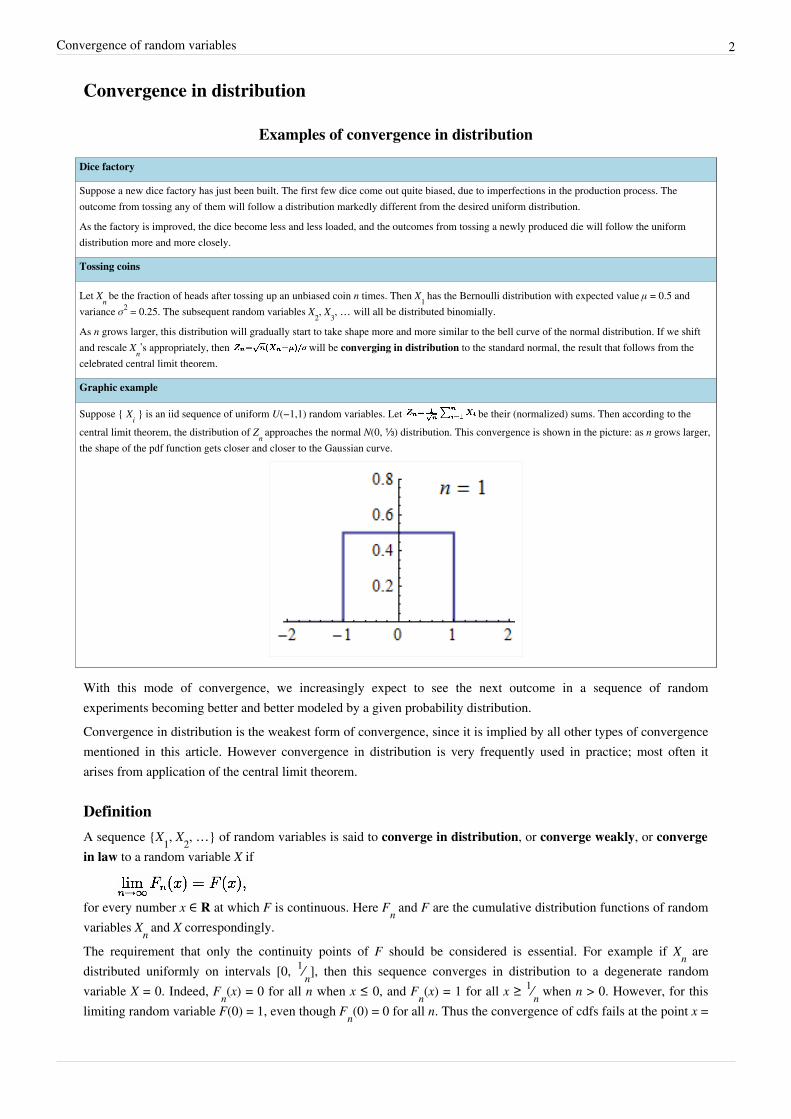
Suppose { Xi } is an iid sequence of uniform U(−1,1) random variables. Let be their (normalized) sums. Then according to thecentral limit theorem, the distribution of Zn approaches the normal N(0, ⅓) distribution. This convergence is shown in the picture: as n grows larger,the shape of the pdf function gets closer and closer to the Gaussian curve.

With this mode of convergence, we increasingly expect to see the next outcome in a sequence of randomexperiments becoming better and better modeled by a given probability distribution.Convergence in distribution is the weakest form of convergence, since it is implied by all other types of convergencementioned in this article. However convergence in distribution is very frequently used in practice; most often itarises from application of the central limit theorem.

DefinitionA sequence {X1, X2, …} of random variables is said to converge in distribution, or converge weakly, or convergein law to a random variable X if

for every number x ∈ R at which F is continuous. Here Fn and F are the cumulative distribution functions of randomvariables Xn and X correspondingly.The requirement that only the continuity points of F should be considered is essential. For example if Xn are distributed uniformly on intervals [0, 1⁄n], then this sequence converges in distribution to a degenerate random variable X = 0. Indeed, Fn(x) = 0 for all n when x ≤ 0, and Fn(x) = 1 for all x ≥ 1⁄n when n > 0. However, for this limiting random variable F(0) = 1, even though Fn(0) = 0 for all n. Thus the convergence of cdfs fails at the point x =

Convergence of random variables 3

0 where F is discontinuous.Convergence in distribution may be denoted as

where is the law (probability distribution) of X. For example if X is standard normal we can write .For random vectors {X1, X2, …} ⊂ Rk the convergence in distribution is defined similarly. We say that this sequenceconverges in distribution to a random k-vector X if

for every A ⊂ Rk which is a continuity set of X.The definition of convergence in distribution may be extended from random vectors to more complex randomelements in arbitrary metric spaces, and even to the “random variables” which are not measurable — a situationwhich occurs for example in the study of empirical processes. This is the “weak convergence of laws without lawsbeing defined” — except asymptotically.[1]

In this case the term weak convergence is preferable (see weak convergence of measures), and we say that asequence of random elements {Xn} converges weakly to X (denoted as Xn ⇒ X) if

for all continuous bounded functions h(·).[2] Here E* denotes the outer expectation, that is the expectation of a“smallest measurable function g that dominates h(Xn)”.

Properties• Since F(a) = Pr(X ≤ a), the convergence in distribution means that the probability for Xn to be in a given range is

approximately equal to the probability that the value of X is in that range, provided n is sufficiently large.• In general, convergence in distribution does not imply that the sequence of corresponding probability density

functions will also converge. As an example one may consider random variables with densitiesƒn(x) = (1 − cos(2πnx))1{x∈(0,1)}. These random variables converge in distribution to a uniform U(0, 1), whereastheir densities do not converge at all.[3]

• Portmanteau lemma provides several equivalent definitions of convergence in distribution. Although thesedefinitions are less intuitive, they are used to prove a number of statistical theorems. The lemma states that {Xn}converges in distribution to X if and only if any of the following statements are true:• Eƒ(Xn) → Eƒ(X) for all bounded, continuous functions ƒ;• Eƒ(Xn) → Eƒ(X) for all bounded, Lipschitz functions ƒ;• limsup{ Eƒ(Xn) } ≤ Eƒ(X) for every upper semi-continuous function ƒ bounded from above;• liminf{ Eƒ(Xn) } ≥ Eƒ(X) for every lower semi-continuous function ƒ bounded from below;• limsup{ Pr(Xn ∈ C) } ≤ Pr(X ∈ C) for all closed sets C;• liminf{ Pr(Xn ∈ U) } ≥ Pr(X ∈ U) for all open sets U;• lim{ Pr(Xn ∈ A) } = Pr(X ∈ A) for all continuity sets A of random variable X.

• Continuous mapping theorem states that for a continuous function g(·), if the sequence {Xn} converges indistribution to X, then so does {g(Xn)} converge in distribution to g(X).

• Lévy’s continuity theorem: the sequence {Xn} converges in distribution to X if and only if the sequence ofcorresponding characteristic functions {φn} converges pointwise to the characteristic function φ of X, and φ(t) iscontinuous at t = 0.

• Convergence in distribution is metrizable by the Lévy–Prokhorov metric.• A natural link to convergence in distribution is the Skorokhod's representation theorem.

Convergence of random variables 4

Convergence in probability

Examples of convergence in probability

Height of a person

Suppose we would like to conduct the following experiment. First, pick a random person in the street. Let X be his/her height, which is ex ante arandom variable. Then you start asking other people to estimate this height by eye. Let Xn be the average of the first n responses. Then (providedthere is no systematic error) by the law of large numbers, the sequence Xn will converge in probability to the random variable X.

Archer

Suppose a person takes a bow and starts shooting arrows at a target. Let Xn be his score in n-th shot. Initially he will be very likely to score zeros,but as the time goes and his archery skill increases, he will become more and more likely to hit the bullseye and score 10 points. After the years ofpractice the probability that he hit anything but 10 will be getting increasingly smaller and smaller. Thus, the sequence Xn converges in probabilityto X = 10.

Note that Xn does not converge almost surely however. No matter how professional the archer becomes, there will always be a small probability ofmaking an error. Thus the sequence {Xn} will never turn stationary: there will always be non-perfect scores in it, even if they are becomingincreasingly less frequent.

The basic idea behind this type of convergence is that the probability of an “unusual” outcome becomes smaller andsmaller as the sequence progresses.The concept of convergence in probability is used very often in statistics. For example, an estimator is calledconsistent if it converges in probability to the quantity being estimated. Convergence in probability is also the type ofconvergence established by the weak law of large numbers.

DefinitionA sequence {Xn} of random variables converges in probability towards X if for all ε > 0

Formally, pick any ε > 0 and any δ > 0. Let Pn be the probability that Xn is outside the ball of radius ε centered at X.Then for Xn to converge in probability to X there should exist a number Nδ such that for all n ≥ Nδ the probability Pnis less than δ.Convergence in probability is denoted by adding the letter p over an arrow indicating convergence, or using the“plim” probability limit operator:

For random elements {Xn} on a separable metric space (S, d), convergence in probability is defined similarly by[4]

Properties• Convergence in probability implies convergence in distribution.[proof]

• Convergence in probability implies almost sure convergence on discrete probability spaces. Since A.S.convergence always implies convergence in probability, in the discrete case, strong convergence and convergencein probability mean the same thing.[proof]

• In the opposite direction, convergence in distribution implies convergence in probability only when the limitingrandom variable X is a constant.[proof]

• The continuous mapping theorem states that for every continuous function g(·), if , then also .• Convergence in probability defines a topology on the space of random variables over a fixed probability space.

This topology is metrizable by the Ky Fan metric:[5]

Convergence of random variables 5

Almost sure convergence

Examples of almost sure convergence

Example 1

Consider an animal of some short-lived species. We note the exact amount of food that this animal consumes day by day. This sequence of numberswill be unpredictable in advance, but we may be quite certain that one day the number will become zero, and will stay zero forever after.

Example 2

Consider a man who starts tomorrow to toss seven coins once every morning. Each afternoon, he donates a random amount of money to a certaincharity. The first time the result is all tails, however, he will stop permanently.

Let X1, X2, … be the day by day amounts the charity receives from him.

We may be almost sure that one day this amount will be zero, and stay zero forever after that.

However, when we consider any finite number of days, there is a nonzero probability the terminating condition will not occur.

This is the type of stochastic convergence that is most similar to pointwise convergence known from elementary realanalysis.

DefinitionTo say that the sequence Xn converges almost surely or almost everywhere or with probability 1 or stronglytowards X means that

This means that the values of Xn approach the value of X, in the sense (see almost surely) that events for which Xndoes not converge to X have probability 0. Using the probability space and the concept of the randomvariable as a function from Ω to R, this is equivalent to the statement

Another, equivalent, way of defining almost sure convergence is as follows:

Almost sure convergence is often denoted by adding the letters a.s. over an arrow indicating convergence:

For generic random elements {Xn} on a metric space (S, d), convergence almost surely is defined similarly:

Properties• Almost sure convergence implies convergence in probability, and hence implies convergence in distribution. It is

the notion of convergence used in the strong law of large numbers.• The concept of almost sure convergence does not come from a topology. This means there is no topology on the

space of random variables such that the almost surely convergent sequences are exactly the converging sequenceswith respect to that topology. In particular, there is no metric of almost sure convergence.

Convergence of random variables 6

Sure convergenceTo say that the sequence or random variables (Xn) defined over the same probability space (i.e., a random process)converges surely or everywhere or pointwise towards X means

where Ω is the sample space of the underlying probability space over which the random variables are defined.This is the notion of pointwise convergence of sequence functions extended to sequence of random variables. (Notethat random variables themselves are functions).

Sure convergence of a random variable implies all the other kinds of convergence stated above, but there is nopayoff in probability theory by using sure convergence compared to using almost sure convergence. The differencebetween the two only exists on sets with probability zero. This is why the concept of sure convergence of randomvariables is very rarely used.

Convergence in meanWe say that the sequence Xn converges in the r-th mean (or in the Lr-norm) towards X, for some r ≥ 1, if r-thabsolute moments of Xn and X exist, and

where the operator E denotes the expected value. Convergence in r-th mean tells us that the expectation of the r-thpower of the difference between Xn and X converges to zero.This type of convergence is often denoted by adding the letter Lr over an arrow indicating convergence:

The most important cases of convergence in r-th mean are:• When Xn converges in r-th mean to X for r = 1, we say that Xn converges in mean to X.• When Xn converges in r-th mean to X for r = 2, we say that Xn converges in mean square to X. This is also

sometimes referred to as convergence in mean, and is sometimes denoted[6]

Convergence in the r-th mean, for r > 0, implies convergence in probability (by Markov's inequality), while if r > s ≥1, convergence in r-th mean implies convergence in s-th mean. Hence, convergence in mean square impliesconvergence in mean.

Convergence in rth-order mean

Examples of convergence in rth-order mean.

Basic example: A newly built factory produces cans of beer. The owners want each can to contain exactly a certain amount.Knowing the details of the current production process, engineers may compute the expected error in a newly produced can.They are continuously improving the production process, so as time goes by, the expected error in a newly produced can tends tozero. This example illustrates convergence in first-order mean.

This is a rather "technical" mode of convergence. We essentially compute a sequence of real numbers, one numberfor each random variable, and check if this sequence is convergent in the ordinary sense.

Convergence of random variables 7

Formal definition

If for some real number a, then {Xn} converges in rth-order mean to a.

Commonly used notation:

PropertiesThe chain of implications between the various notions of convergence are noted in their respective sections. Theyare, using the arrow notation:

These properties, together with a number of other special cases, are summarized in the following list:• Almost sure convergence implies convergence in probability:[7] [proof]

• Convergence in probability implies there exists a sub-sequence which almost surely converges:[8]

• Convergence in probability implies convergence in distribution:[7] [proof]

• Convergence in r-th order mean implies convergence in probability:

• Convergence in r-th order mean implies convergence in lower order mean, assuming that both orders are greaterthan one:

provided r ≥ s ≥ 1.• If Xn converges in distribution to a constant c, then Xn converges in probability to c:[7] [proof]

provided c is a constant.• If Xn converges in distribution to X and the difference between Xn and Yn converges in probability to zero, then Yn

also converges in distribution to X:[7] [proof]

• If Xn converges in distribution to X and Yn converges in distribution to a constant c, then the joint vector (Xn, Yn)converges in distribution to (X, c):[7] [proof]

provided c is a constant.Note that the condition that Yn converges to a constant is important, if it were to converge to a random variable Ythen we wouldn’t be able to conclude that (Xn, Yn) converges to (X, Y).

• If Xn converges in probability to X and Yn converges in probability to Y, then the joint vector (Xn, Yn) converges inprobability to (X, Y):[7] [proof]

• If Xn converges in probability to X, and if P(|Xn| ≤ b) = 1 for all n and some b, then Xn converges in rth mean to Xfor all r ≥ 1. In other words, if Xn converges in probability to X and all random variables Xn are almost surelybounded above and below, then Xn converges to X also in any rth mean.

• Almost sure representation. Usually, convergence in distribution does not imply convergence almost surely.However for a given sequence {Xn} which converges in distribution to X0 it is always possible to find a newprobability space (Ω, F, P) and random variables {Yn, n = 0,1,…} defined on it such that Yn is equal indistribution to Xn for each n ≥ 0, and Yn converges to Y0 almost surely.[9]

Convergence of random variables 8

• If for all ε > 0,

then we say that Xn converges almost completely, or almost in probability towards X. When Xn convergesalmost completely towards X then it also converges almost surely to X. In other words, if Xn converges inprobability to X sufficiently quickly (i.e. the above sequence of tail probabilities is summable for all ε > 0),then Xn also converges almost surely to X. This is a direct implication from the Borel-Cantelli lemma.

• If Sn is a sum of n real independent random variables:

then Sn converges almost surely if and only if Sn converges in probability.• The dominated convergence theorem gives sufficient conditions for almost sure convergence to imply

L1-convergence:

• A necessary and sufficient condition for L1 convergence is and the sequence (Xn) is uniformlyintegrable.

Notes[1] Bickel et al. 1998, A.8, page 475[2] van der Vaart & Wellner 1996, p. 4[3] Romano & Siegel 1985, Example 5.26[4] Dudley 2002, Chapter 9.2, page 287[5] Dudley 2002, p. 289[6] Porat, B. (1994). Digital Processing of Random Signals: Theory & Methods. Prentice Hall. pp. 19. ISBN 0130637513.[7] van der Vaart 1998, Theorem 2.7[8] Gut, Allan (2005). Probability: A graduate course. Theorem 3.4: Springer. ISBN 0387228330.[9] van der Vaart 1998, Th.2.19

References• Bickel, Peter J.; Klaassen, Chris A.J.; Ritov, Ya’acov; Wellner, Jon A. (1998). Efficient and adaptive estimation

for semiparametric models. New York: Springer-Verlag. ISBN 0387984739. LCCN QA276.8.E374.• Billingsley, Patrick (1986). Probability and Measure. Wiley Series in Probability and Mathematical Statistics

(2nd ed.). Wiley.• Billingsley, Patrick (1999). Convergence of probability measures (2nd ed.). John Wiley & Sons. pp. 1–28.

ISBN 0471197459.• Dudley, R.M. (2002). Real analysis and probability. Cambridge, UK: Cambridge University Press.

ISBN 052180972X.• Grimmett, G.R.; Stirzaker, D.R. (1992). Probability and random processes (2nd ed.). Clarendon Press, Oxford.

pp. 271–285. ISBN 0-19-853665-8.• Jacobsen, M. (1992). Videregående Sandsynlighedsregning (Advanced Probability Theory) (3rd ed.). HCØ-tryk,

Copenhagen. pp. 18–20. ISBN 87-91180-71-6.• Ledoux, Michel; Talagrand, Michel (1991). Probability in Banach spaces. Berlin: Springer-Verlag. pp. xii+480.

ISBN 3-540-52013-9. MR1102015.

Convergence of random variables 9

• Romano, Joseph P.; Siegel, Andrew F. (1985). Counterexamples in probability and statistics. Great Britain:Chapman & Hall. ISBN 0412989018. LCCN QA273.R58 1985.

• van der Vaart, Aad W.; Wellner, Jon A. (1996). Weak convergence and empirical processes. New York:Springer-Verlag. ISBN 0387946403. LCCN QA274.V33 1996.

• van der Vaart, Aad W. (1998). Asymptotic statistics. New York: Cambridge University Press.ISBN 9780521496032. LCCN QA276.V22 1998.

• Williams, D. (1991). Probability with Martingales. Cambridge University Press. ISBN 0521406056.• Wong, E.; Hájek, B. (1985). Stochastic Processes in Engineering Systems. New York: Springer–Verlag.This article incorporates material from the Citizendium article "Stochastic convergence", which is licensed underthe Creative Commons Attribution-ShareAlike 3.0 Unported License but not under the GFDL.

Article Sources and Contributors 10

Article Sources and ContributorsConvergence of random variables  Source: http://en.wikipedia.org/w/index.php?oldid=457408351  Contributors: A. Pichler, Aastrup, Albmont, Amir Aliev, Andrea Ambrosio, Ardonik,AxelBoldt, Bjcairns, CALR, Cenarium, Chungc, Constructive editor, DHN, David Eppstein, Deepakr, Derveish, Ensign beedrill, Fpoursafaei, Fram, GaborPete, Giftlite, Headbomb, HyDeckar,Igny, J04n, JA(000)Davidson, JamesBWatson, Jmath666, Jncraton, Josh Guffin, Josh Parris, Kolesarm, Kri, Landroni, LoveOfFate, McKay, Melcombe, Mets501, Michael Hardy, Notedgrant,Oleg Alexandrov, Paul August, Philtime, PigFlu Oink, Prewitt81, Qwfp, Ricardogpn, Robin S, Robinh, Sam Hocevar, Sligocki, Spireguy, Steve Kroon, Stigin, Stpasha, Sullivan.t.j, Szepi,TedPavlic, The Mad Echidna, Voorlandt, Wartoilet, Weierstraß, Zvika, 107 anonymous edits

Image Sources, Licenses and ContributorsImage:Convergence in distribution (sum of uniform rvs).gif  Source: http://en.wikipedia.org/w/index.php?title=File:Convergence_in_distribution_(sum_of_uniform_rvs).gif  License: CreativeCommons Zero  Contributors: Stpasha

LicenseCreative Commons Attribution-Share Alike 3.0 Unported//creativecommons.org/licenses/by-sa/3.0/

Convergence of measures 1

Convergence of measuresIn mathematics, more specifically measure theory, there are various notions of the convergence of measures. Threeof the most common notions of convergence are described below.

Total variation convergence of measuresThis is the strongest notion of convergence shown on this page and is defined a follows. Let be ameasurable space. The total variation distance between two (positive) measures and is then given by

If and are both probability measures, then the total variation distance is also given by

The equivalence between these two definitions can be seen as a particular case of the Monge-Kantorovich duality.From the two definitions above, it is clear that the total variation distance between probability measures is alwaysbetween 0 and 2.To illustrate the meaning of the total variation distance, consider the following thought experiment. Assume that weare given two probability measures and , as well as a random variable . We know that has law either

or , but we do not know which one of the two. Assume now that we are given one single sample distributedaccording to the law of and that we are then asked to guess which one of the two distributions describes that law.The quantity

then provides a sharp upper bound on the probability that our guess is correct.

Strong convergence of measuresFor a measurable space, a sequence is said to converge strongly to a limit if

for every set in .For example, as a consequence of the Riemann–Lebesgue lemma, the sequence of measures on the interval[-1,1] given by converges strongly to Lebesgue measure, but it does not convergein total variation.

Weak convergence of measuresIn mathematics and statistics, weak convergence (also known as narrow convergence or weak-* convergencewhich is a more appropriate name from the point of view of functional analysis but less frequently used) is one ofmany types of convergence relating to the convergence of measures. It depends on a topology on the underlyingspace and thus is not a purely measure theoretic notion.There are several equivalent definitions of weak convergence of a sequence of measures, some of which are(apparently) more general than others. The equivalence of these conditions is sometimes known as the portmanteautheorem.Definition. Let S be a metric space with its Borel σ-algebra Σ. We say that a sequence of probability measures on (S,Σ), Pn, n = 1, 2, ..., converges weakly to the probability measure P, and write

Convergence of measures 2

if any of the following equivalent conditions is true:• Enƒ → Eƒ for all bounded, continuous functions ƒ;• Enƒ → Eƒ for all bounded and Lipschitz functions ƒ;• limsup Enƒ ≤ Eƒ for every upper semi-continuous function ƒ bounded from above;• liminf Enƒ ≥ Eƒ for every lower semi-continuous function ƒ bounded from below;• limsup Pn(C) ≤ P(C) for all closed sets C of space S;• liminf Pn(U) ≥ P(U) for all open sets U of space S;• lim Pn(A) = P(A) for all continuity sets A of measure P.In the case S = R with its usual topology, if Fn, F denote the cumulative distribution functions of the measures Pn, Prespectively, then Pn converges weakly to P if and only if limn→∞ Fn(x) = F(x) for all points x ∈ R at which F iscontinuous.For example, the sequence where Pn is the Dirac measure located at 1/n converges weakly to the Dirac measurelocated at 0 (if we view these as measures on R with the usual topology), but it does not converge strongly. This isintuitively clear: we only know that 1/n is "close" to 0 because of the topology of R.This definition of weak convergence can be extended for S any metrizable topological space. It also defines a weaktopology on P(S), the set of all probability measures defined on (S, Σ). The weak topology is generated by thefollowing basis of open sets:

where

If S is also separable, then P(S) is metrizable and separable, for example by the Lévy–Prokhorov metric, if S is alsocompact or Polish, so is P(S).If S is separable, it naturally embeds into P(S) as the (closed) set of dirac measures, and its convex hull is dense.There are many "arrow notations" for this kind of convergence: the most frequently used are , and .

Weak convergence of random variables

Let be a probability space and X be a metric space. If Xn, X: Ω → X is a sequence of random variablesthen Xn is said to converge weakly (or in distribution or in law) to X as n → ∞ if the sequence of pushforwardmeasures (Xn)∗(P) converges weakly to X∗(P) in the sense of weak convergence of measures on X, as defined above.

References• Ambrosio, L., Gigli, N. & Savaré, G. (2005). Gradient Flows in Metric Spaces and in the Space of Probability

Measures. Basel: ETH Zürich, Birkhäuser Verlag. ISBN 3-7643-2428-7.• Billingsley, Patrick (1995). Probability and Measure. New York, NY: John Wiley & Sons, Inc..

ISBN 0-471-00710-2.• Billingsley, Patrick (1999). Convergence of Probability Measures. New York, NY: John Wiley & Sons, Inc..

ISBN 0-471-19745-9.

Article Sources and Contributors 3

Article Sources and ContributorsConvergence of measures  Source: http://en.wikipedia.org/w/index.php?oldid=460030246  Contributors: Derveish, Diegotorquemada, Hairer, Igny, J04n, Melcombe, Michael Hardy, PaulAugust, Radagast83, Stpasha, Sullivan.t.j, Thenub314, 13 anonymous edits

LicenseCreative Commons Attribution-Share Alike 3.0 Unported//creativecommons.org/licenses/by-sa/3.0/