MASTER THESIS
THESIS PROJECT Master program in Computer science
Author
Salar Askar Zada
2010-08-23
Ad Hoc Networks: Performance Evaluation Of Proactive, Reactive And
Hybrid Routing Protocols In NS2
MASTER THESIS
Abstract
No infrastructure, no centralized administration and self-configuration are the main characteristics of
MANETs. The primary motivation of MANET deployment is to increase portability, mobility and flexibility.
However, this mobility causes an unpredictable change in topology and makes routing more difficult. Many
routing algorithms have been proposed and tested over the last few years in order to provide an efficient
routing in Ad Hoc networks. In this report we will show our conducted study with AODV (reactive), DSDV
(proactive) and ZRP (hybrid) routing protocols. The performance of routing protocols have been evaluated
carefully by analyzing the affects of changing network parameters such as, number of nodes, velocity, pause
time, workload and flows on three performance metrics: packet delivery ratio, routing cost and average end-
to- end delay. All the simulation work has been conducted in NS2. Our simulation results show that AODV
gives better performance in all designed simulation models in terms of packets delivery ratio. DSDV shows the
second best performance. Performance of ZRP is found average.
Date: August, 23, 2010
Author: Salar Askar Zada
Examiner: Thomas Lundqvist
Advisor: Dr. Stanislav Belenki
Programmed: Masters in Computer Science
Main field of study: Computer Networks
Education level: Second cycle
Credits: 15 HE credits
Course code: EXD908
Keywords Introduction, Background, Methodology, Simulation results and analysis, Comparison and discussion, Conclusion
Publisher: University West, Department of Economics and IT SE-461 86 Trollhättan, SWEDEN Phone: + 46 520 22 30 00 Fax: + 46 520 22 32 99 Web: www.hv.se
MASTER THESIS
Preface
This thesis is simulation based research work in Ad Hoc network’s routing protocols which is submitted to
University West for the fulfillment of Master degree. Three categories of Ad Hoc routing protocol techniques
(proactive, reactive and hybrid) are investigated in five different models. Thesis provides clear knowledge of
difference, similarities and issues related to routing in Ad Hoc networks. A detailed discussion on the results has
been provided in section five of this report.
I specially want to thanks my supervisor Dr. Stanislav Belenki for his guidance and literary support. There may
be some errors in writing in this report for that I take complete responsibility. I am also grateful to faculty of
Department of Economics and IT for allowing me to do this work. I also would like to thank my friend Mr. Yasser,
who helped me installing and configuring Zone routing protocol in NS2. Finally I would like to thanks to my parents
for their financial and moral support.
MASTER THESIS
1. INTRODUCTION Mobile Ad Hoc Wireless Networks (MANETs) are said to
be future networks and have been receiving attention during
the last few years [1]. This popularity of MANET is because
of wide range of available wireless services providing
ubiquitous computing at low cost [2].
A MANET is self-organizing and infrastructure less
system. Mobile routers (nodes) can establish network
connections anytime. The primary goal of such type of
network is to provide rapid means of communication,
computing and deployment [3]. Each mobile node in Ad Hoc
network is capable of routing packets and assists neighboring
nodes to do so. In this dynamically changing topology
environment the role of routing protocols are very significant.
Over the last two decades several routing protocols have been
proposed. Such as: AODV, DSR, DSDV, OLSR, TORA and
ZRP. The unique feature of these routing protocols is the
ability to route packets in dynamic topology [4]. This
dynamic environment not only gives big challenges to
improve the performance of routing protocols but also invites
researchers to consider the network architecture at almost
every layer from physical layer to medium access control [3].
There are several factors which affect the performance of
Ad Hoc network routing protocols. For instance, node’s
varying speed may cause link failure. Network size and traffic
load may cause congestion. Limited transmission range,
bandwidth and battery power also make considerable impacts
on network scalability. [3]
In most of the conducted researches the comparisons have
been made between reactive and proactive protocols. The
motivation of conducting this research is to provide a
comprehensive performance comparison amongst reactive,
proactive and hybrid routing protocols. For this purpose we
selected the protocols from each category i.e. AODV
(reactive), DSDV (proactive) and ZRP (hybrid). In order to
evaluate the performance we performed intensive simulation
in NS2 and tested every protocol in five different models with
changing network parameters.
Latter in this report we will present our understanding and
observation of how selected performance metrics (packets
delivery fraction, average end-to-end network delay and
routing cost) are affected by changing network parameters.
This report is organized as: section 2 is background study
of routing protocols. Section 3 is methodology section, where
the framework of simulator, routing metrics, testing models
and simulation environment are defined. In section 4, we
described and analyzed the simulation results. A detail
comparative discussion of simulation results is presented in
section 5. Finally report ends in section 6 with conclusion.
Keywords: AODV, DSDV, ZRP, Mobile Ad Hoc Network, and NS-2.
2. BACKGROUND
Due to different routing techniques, mobile Ad Hoc
protocols can be classified in to proactive (table-driven),
reactive (on-demand) and hybrid (mix features of proactive
and reactive routing). The following section further describes
these routing techniques and routing protocols.
Reactive routing protocol: also called on-demand routing
protocols. In on-demand routing, routes are only created
and maintained when needed. Route discovery mechanism
is used to find path. Path to the destination remains
maintained until no longer needed or become inaccessible.
AODV and DSR fall into this category.
Proactive routing protocol: also called table-driven
protocols. Such protocols keep updated routing information
at each node in the network. DSDV, OLSR and WRP fall
into this category.
Hybrid routing protocols: these routing protocols have the
features of both proactive and reactive routing. An example
of such protocol is ZRP.
Based on the above stated routing strategies a variety of
routing protocols have been developed so far. As far as the
scope of this thesis is concern, we will describe three ad hoc
routing protocols: AODV, DSDV and ZRP.
Ad Hoc On-Demand Distance Vector Routing Protocol
The Ad Hoc On-Demand Distance Vector (AODV) [5] is
reactive routing protocol. AODV also called source-initiated
routing algorithm, because AODV only discovers the path to
the destination when source wants to send data. Established
path between source and destination remains as long as it is
needed or becomes inaccessible. Route discovery mechanism
of AODV is based on route request (RREQ), route reply
(RREP), and route error (RERR) messages. Since AODV is
flooding in nature, when there is need to discover path,
source node floods RREQ message to all neighboring nodes.
This RREQ message contains destination sequence number.
This sequence number helps in ensuring route validity and
prevents routing loops [6]. For example, a route with greatest
sequence number is always chosen by sending node. After
receiving RREQ message each neighboring node checks the
destination ID. When the path is found, RREP message is
sent back to requesting node. The path followed by RREP
message is used to send data packet. On the other hand, when
the path is not found, neighboring nodes forward the RREQ
to their neighbors. In case of link breaks a RERR message is
sent to source node informing that link is no longer valid
now. The route discovery mechanism of AODV is similar to
DSR and routing table of AODV with destination sequence
numbers is similar to DSDV [7].
Destination Sequence Distance Vector Protocol
The Destination Sequence Distance Vector (DSDV) [7] is
proactive routing protocol. DSDV also called table-driven
routing protocol because each node maintains routing table
that contains sequence numbers and hope-by-hope
information. DSDV is based on Bellman-Ford routing
MASTER THESIS
algorithm. Some major improvements have been made in
Bellman-Ford algorithm in order to make it suitable for
wireless environment and cope with count-to-infinity
problem. DSDV uses the sequence number to avoid count-to-
infinity problem and using this sequence number DSDV
distinguishes between stale and fresh routes. Nodes talk with
each other’s and update their routing tables. If change in
topology occurs updates are transmitted. There are two types
of updates, time-driven (periodic updates) and table- driven
(updates because of significant change). In case of any
change, routing updates are transmitted to all other nodes
which may cause large overhead. In order to reduce this
overhead routing updates are sent in two ways: a full dump
way, where full routing table is sent to neighbors but it
happens only in case of complete topology change. An
incremental update: where only the entries change in the
route metric are sent. [6, 7]
Zone Routing Protocol
ZRP is designed to address the problems associated with
proactive and reactive routing. Excess bandwidth
consumption because of flooding of updates packets and long
delay in route discovery request are two main problems of
proactive and reactive routing respectively. ZRP came with
the concept of zones. In limited zone, route maintenance is
easier and because of zones, numbers of routing updates are
decreased. Nodes out of the zone can communicate via
reactive routing, for this purpose route request is not flooded
to entire network only the border node is responsible to
perform this task. ZRP combines the feature of both proactive
and reactive routing algorithms [10]. The architecture of ZRP
consists of four elements: MAC-level functions, Intra-Zone
Routing Protocol (IARP), Inter-Zone Routing Protocol (IERP)
and Bordercast Routing Protocol (BRP). The proactive
routing is used within limited specified zones and beyond the
zones reactive routing is used. MAC-level performs neighbor
discovery and maintenance functions. For instance, when a
node comes in range a notification of new neighbor is sent to
IARP similarly when node losses connectivity, lost
connectivity notification is sent to IARP. Within in a
specified zone, IARP protocol routes packets. IARP keeps
information about all nodes in the zone in its routing table.
On the other hand, if node wants to send packet to a node
outside the zone, in that case IERP protocol is used to find
best path. That means IERP is responsible to maintains
correct routes outside the zone. If IERP does not have any
route in its routing table, it sends route query to BRP. The
BRP is responsible to contact with nodes across Ad Hoc
networks and passes route queries. Important thing in
bordercasting mechanism of BRP is it avoids packets flood in
network. BRP always passes route query request to border
nodes only, since only border nodes transmit and receive
packets. [8, 9, 10]
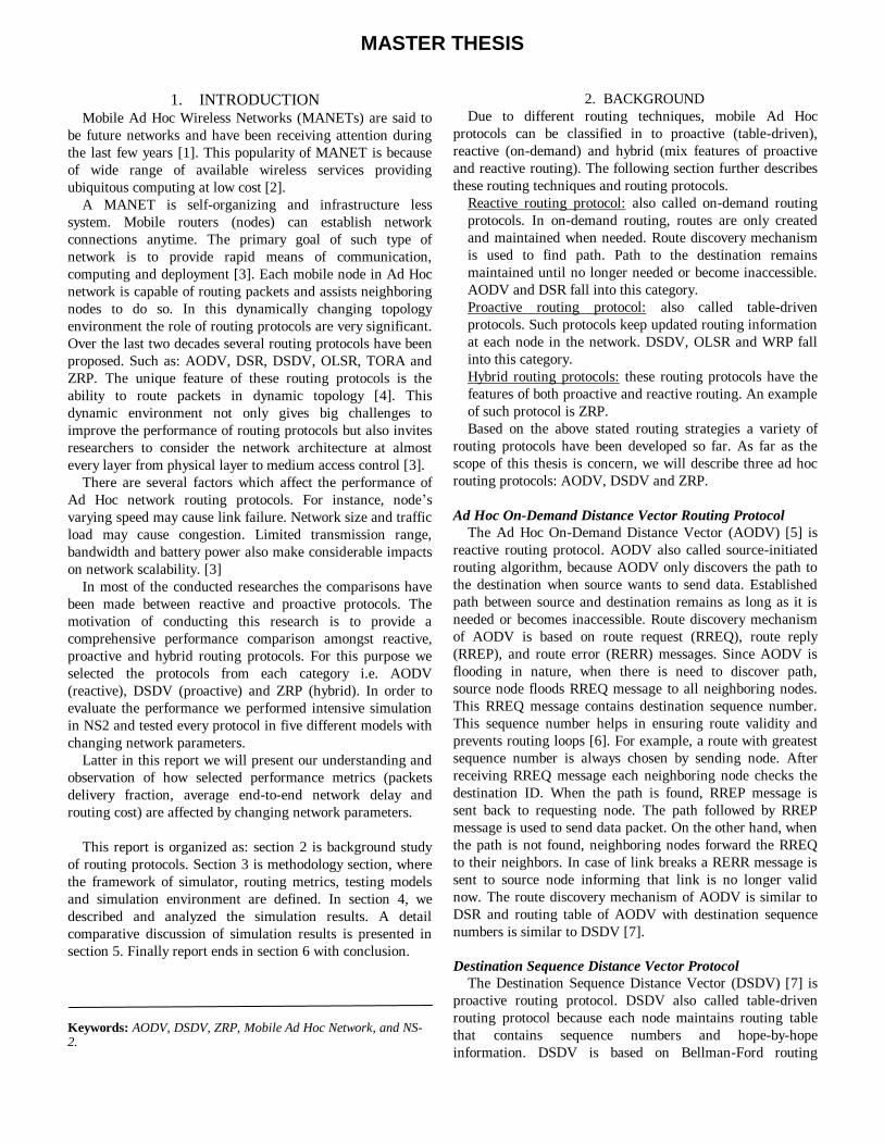
Figure 1: shows a simple topology of zone radius of 2
nodes for query node A. The border nodes are E, F and G. if
we take zone radius 1, the nodes B, C and D will be border
nodes and for zone radius 3, nodes H and I will become
border nodes in this topology.
Query Node A
D
Border
Nodes E,
I
F and G
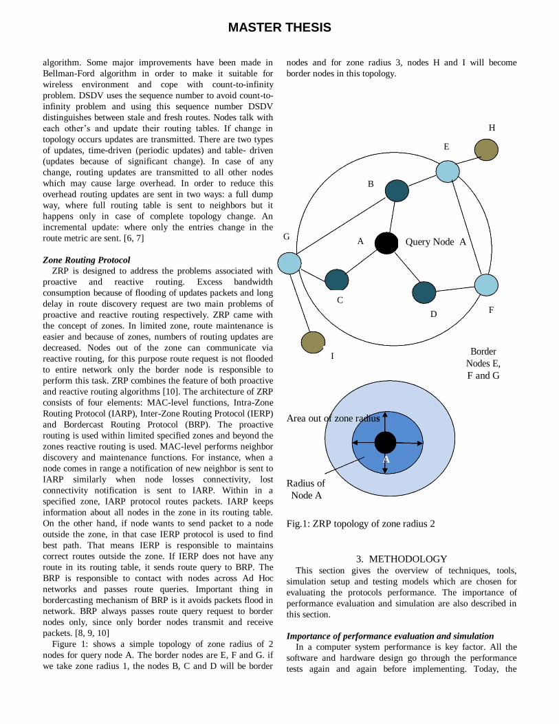
Area out of zone radius
A
Radius of
Node A Fig.1: ZRP topology of zone radius 2
3. METHODOLOGY This section gives the overview of techniques, tools,
simulation setup and testing models which are chosen for
evaluating the protocols performance. The importance of
performance evaluation and simulation are also described in
this section.
Importance of performance evaluation and simulation
In a computer system performance is key factor. All the
software and hardware design go through the performance
tests again and again before implementing. Today, the
A
B
E
F C
D
H
I
G
MASTER THESIS
corporate word heavily depends upon computer networks.
Integration of computer system in almost every walk of life
demands a reliable computer network system. It is therefore
considers necessary for all computer professionals,
researchers and system engineers to acquire basic knowledge
of performance evaluating technique. [12]
Performance can be evaluated via measurement, modeling
and simulation. In this thesis, performance evaluation based
on simulation rather analytical modeling. Simulation
technique is suitable for testing models especially in research
areas and educational centers. Potential advantages of
simulation are, it saves time, cost and provides detail results
and good understanding of event’s occurrence.
Network simulator
There are many simulators such as OPNET, NetSim,
GloMoSim and NS2 etc. We used NS2 [11] for simulation.
NS2 is quite difficult to use for first time user but once user
get to know the simulator it becomes fairly easy.
NS2 is a discrete event simulator developed at UC Berkeley
and written in C++ and OTcl. Primarily, NS2 was useful for
simulating LAN and WAN only. Multi-hop wireless network
simulation support is provided by the Monarch Research
Group at Carnegie-Mellon University. For wireless
simulation, it contains physical, data link and medium access
control layer. The Distributed Coordination Function (DCF)
of IEEE 802.11 for wireless LANs is used as MAC layer
protocol. For transmitting data packets, an Unslotted Carrier
Sense Multiple Access with Collision Avoidance (CSMA/CA)
is used. Radio model is similar to commercial radio interface,
Lucent’s wave LAN. Wave LAN has a share-media radio
with a nominal bit rate of 2 Mb/s and a nominal radio range
of 250m. [7, 11]
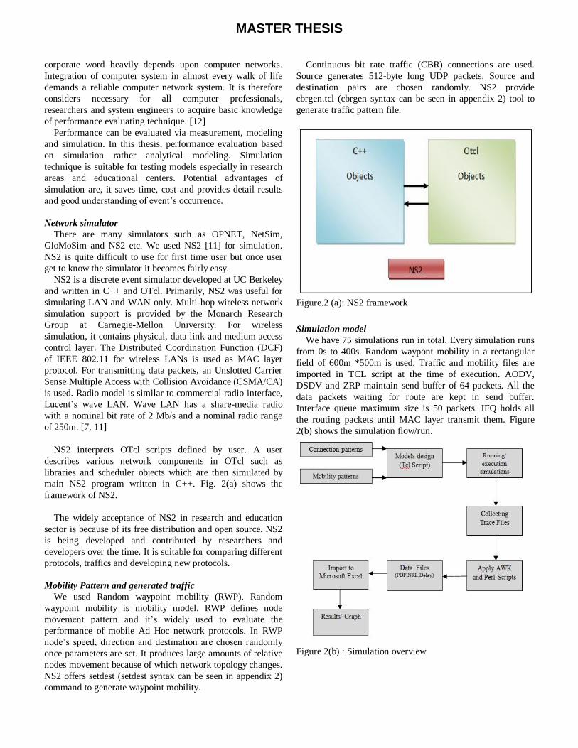
NS2 interprets OTcl scripts defined by user. A user
describes various network components in OTcl such as
libraries and scheduler objects which are then simulated by
main NS2 program written in C++. Fig. 2(a) shows the
framework of NS2.
The widely acceptance of NS2 in research and education
sector is because of its free distribution and open source. NS2
is being developed and contributed by researchers and
developers over the time. It is suitable for comparing different
protocols, traffics and developing new protocols.
Mobility Pattern and generated traffic
We used Random waypoint mobility (RWP). Random
waypoint mobility is mobility model. RWP defines node
movement pattern and it’s widely used to evaluate the
performance of mobile Ad Hoc network protocols. In RWP
node’s speed, direction and destination are chosen randomly
once parameters are set. It produces large amounts of relative
nodes movement because of which network topology changes.
NS2 offers setdest (setdest syntax can be seen in appendix 2)
command to generate waypoint mobility.
Continuous bit rate traffic (CBR) connections are used.
Source generates 512-byte long UDP packets. Source and
destination pairs are chosen randomly. NS2 provide
cbrgen.tcl (cbrgen syntax can be seen in appendix 2) tool to
generate traffic pattern file.
Figure.2 (a): NS2 framework
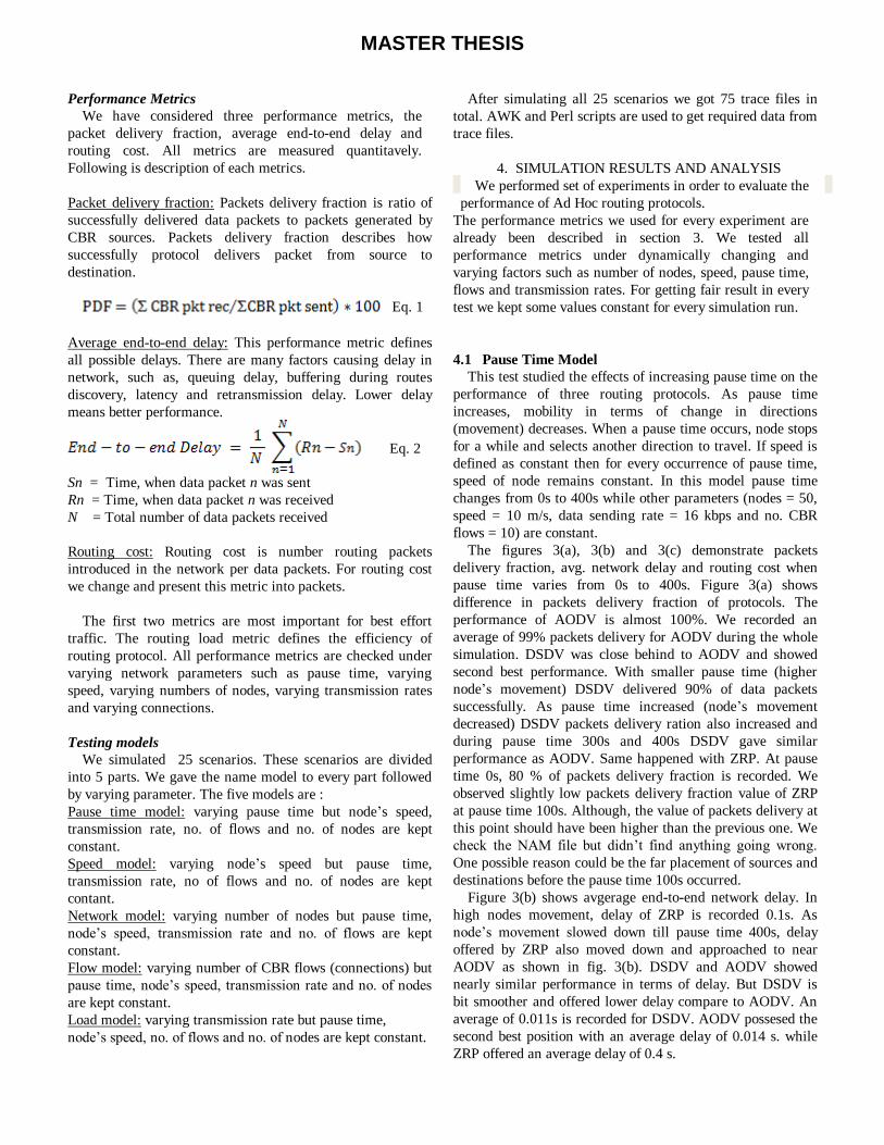
Simulation model
We have 75 simulations run in total. Every simulation runs
from 0s to 400s. Random waypont mobility in a rectangular
field of 600m *500m is used. Traffic and mobility files are
imported in TCL script at the time of execution. AODV,
DSDV and ZRP maintain send buffer of 64 packets. All the
data packets waiting for route are kept in send buffer.
Interface queue maximum size is 50 packets. IFQ holds all
the routing packets until MAC layer transmit them. Figure
2(b) shows the simulation flow/run.
Figure 2(b) : Simulation overview
MASTER THESIS
Performance Metrics
We have considered three performance metrics, the
packet delivery fraction, average end-to-end delay and
routing cost. All metrics are measured quantitavely.
Following is description of each metrics.
Packet delivery fraction: Packets delivery fraction is ratio of
successfully delivered data packets to packets generated by
CBR sources. Packets delivery fraction describes how
successfully protocol delivers packet from source to
destination.
Eq. 1
Average end-to-end delay: This performance metric defines
all possible delays. There are many factors causing delay in
network, such as, queuing delay, buffering during routes
discovery, latency and retransmission delay. Lower delay
means better performance.
Sn = Time, when data packet n was sent
Rn = Time, when data packet n was received
N = Total number of data packets received
Routing cost: Routing cost is number routing packets
introduced in the network per data packets. For routing cost
we change and present this metric into packets.
The first two metrics are most important for best effort
traffic. The routing load metric defines the efficiency of
routing protocol. All performance metrics are checked under
varying network parameters such as pause time, varying
speed, varying numbers of nodes, varying transmission rates
and varying connections.
Testing models
We simulated 25 scenarios. These scenarios are divided
into 5 parts. We gave the name model to every part followed
by varying parameter. The five models are :
Pause time model: varying pause time but node’s speed,
transmission rate, no. of flows and no. of nodes are kept
constant.
Speed model: varying node’s speed but pause time,
transmission rate, no of flows and no. of nodes are kept
contant.
Network model: varying number of nodes but pause time,
node’s speed, transmission rate and no. of flows are kept
constant.
Flow model: varying number of CBR flows (connections) but
pause time, node’s speed, transmission rate and no. of nodes
are kept constant.
Load model: varying transmission rate but pause time,
node’s speed, no. of flows and no. of nodes are kept constant.
After simulating all 25 scenarios we got 75 trace files in
total. AWK and Perl scripts are used to get required data from
trace files.
4. SIMULATION RESULTS AND ANALYSIS
We performed set of experiments in order to evaluate the
performance of Ad Hoc routing protocols.
The performance metrics we used for every experiment are
already been described in section 3. We tested all
performance metrics under dynamically changing and
varying factors such as number of nodes, speed, pause time,
flows and transmission rates. For getting fair result in every
test we kept some values constant for every simulation run.
4.1 Pause Time Model
This test studied the effects of increasing pause time on the
performance of three routing protocols. As pause time
increases, mobility in terms of change in directions
(movement) decreases. When a pause time occurs, node stops
for a while and selects another direction to travel. If speed is
defined as constant then for every occurrence of pause time,
speed of node remains constant. In this model pause time
changes from 0s to 400s while other parameters (nodes = 50,
speed = 10 m/s, data sending rate = 16 kbps and no. CBR
flows = 10) are constant.
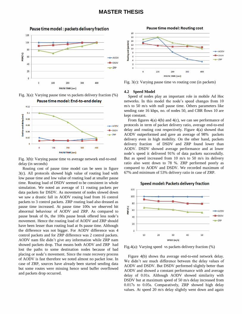
The figures 3(a), 3(b) and 3(c) demonstrate packets
delivery fraction, avg. network delay and routing cost when
pause time varies from 0s to 400s. Figure 3(a) shows
difference in packets delivery fraction of protocols. The
performance of AODV is almost 100%. We recorded an
average of 99% packets delivery for AODV during the whole
simulation. DSDV was close behind to AODV and showed
second best performance. With smaller pause time (higher
node’s movement) DSDV delivered 90% of data packets
successfully. As pause time increased (node’s movement
decreased) DSDV packets delivery ration also increased and
during pause time 300s and 400s DSDV gave similar
performance as AODV. Same happened with ZRP. At pause
time 0s, 80 % of packets delivery fraction is recorded. We
observed slightly low packets delivery fraction value of ZRP
at pause time 100s. Although, the value of packets delivery at
this point should have been higher than the previous one. We
check the NAM file but didn’t find anything going wrong.
One possible reason could be the far placement of sources and
destinations before the pause time 100s occurred.
Figure 3(b) shows avgerage end-to-end network delay. In
high nodes movement, delay of ZRP is recorded 0.1s. As
node’s movement slowed down till pause time 400s, delay
offered by ZRP also moved down and approached to near
AODV as shown in fig. 3(b). DSDV and AODV showed
nearly similar performance in terms of delay. But DSDV is
bit smoother and offered lower delay compare to AODV. An
average of 0.011s is recorded for DSDV. AODV possesed the
second best position with an average delay of 0.014 s. while
ZRP offered an average delay of 0.4 s.
Eq. 2
MASTER THESIS
Fig. 3(a): Varying pause time vs packets delivery fraction (%)
Fig. 3(b): Varying pause time vs average network end-to-end
delay (in seconds)
Routing cost of pause time model can be seen in figure
3(c). All protocols showed high value of routing load with
low pasue time and low value of routing load at smaller pause
time. Routing load of DSDV seemed to be consistent in whole
simulation. We noted an average of 11 routing packets per
data packets for DSDV. As movement of nodes slowed down
we saw a drastic fall in AODV rouing load from 16 control
packets to 3 control packets. ZRP routing load also dreased as
pause time increased. At pause time 100s we observed bit
abnormal behaviour of AODV and ZRP. As compared to
pause break of 0s, the 100s pause break offered less node’s
movement. Hence the routing load of AODV and ZRP should
have been lesser than routing load at 0s pause time. Although
the difference was not bigger. For AODV difference was 4
control packets and for ZRP difference was 2 control packets.
AODV nam file didn’t give any information while ZRP nam
showed packets drop. That means both AODV and ZRP had
lost the paths to some destination nodes because of bad
placing or node’s movement. Since the route recovery process
of AODV is fast therefore we noted almost no packet lose. In
case of ZRP, sources have already been started sending data
but some routes were missing hence send buffer overflowed
and packets drop occurred.
Fig. 3(c): Varying pause time vs routing cost (in packets)
4.2 Speed Model
Speed of nodes play an important role in mobile Ad Hoc
networks. In this model the node’s speed changes from 10
m/s to 50 m/s with null pause time. Others parameters like
sending rate 16 kbps, no. of nodes 50, and CBR flows 10 are
kept constant.
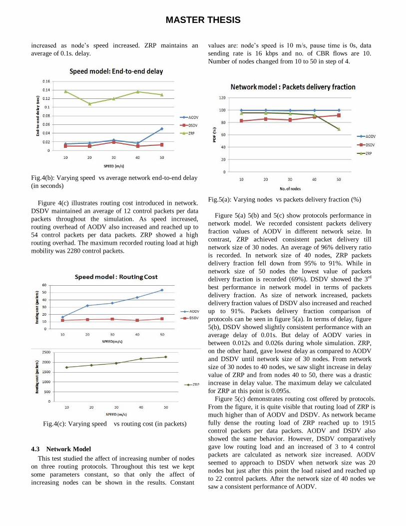
From figures 4(a) 4(b) and 4(c), we can see performance of
protocols in term of packet delivery ratio, average end-to-end
delay and routing cost respectively. Figure 4(a) showed that
AODV outperformed and gave an average of 98% packets
delivery even in high mobility. On the other hand, packets
delivery fraction of DSDV and ZRP found lower than
AODV. DSDV showed average performance and at lower
node’s speed it delivered 91% of data packets successfully.
But as speed increased from 10 m/s to 50 m/s its delivery
ratio also went down to 78 %. ZRP performed poorly as
compared to AODV and DSDV. We recorded maximum of
67% and minimum of 53% delivery ratio in case of ZRP.
Fig.4(a): Varying speed vs packets delivery fraction (%)
Figure 4(b) shows tha average end-to-end network delay.
We didn’t see much difference between the delay values of
AODV and DSDV. But DSDV performed slightly better than
AODV and showed a constant performance with and average
delay of 0.01s. Although AODV showed similarity with
DSDV but at maximum speed of 50 m/s delay increased from
0.017s to 0.05s. Comparatively, ZRP showed high delay
values. At speed 20 m/s delay slightly went down and again
MASTER THESIS
increased as node’s speed increased. ZRP maintains an
average of 0.1s. delay.
Fig.4(b): Varying speed vs average network end-to-end delay
(in seconds)
Figure 4(c) illustrates routing cost introduced in network.
DSDV maintained an average of 12 control packets per data
packets throughout the simulation. As speed increased,
routing overhead of AODV also increased and reached up to
54 control packets per data packets. ZRP showed a high
routing overhad. The maximum recorded routing load at high
mobility was 2280 control packets.
Fig.4(c): Varying speed vs routing cost (in packets)
4.3 Network Model This test studied the affect of increasing number of nodes
on three routing protocols. Throughout this test we kept
some parameters constant, so that only the affect of
increasing nodes can be shown in the results. Constant
values are: node’s speed is 10 m/s, pause time is 0s, data
sending rate is 16 kbps and no. of CBR flows are 10.
Number of nodes changed from 10 to 50 in step of 4.
Fig.5(a): Varying nodes vs packets delivery fraction (%)
Figure 5(a) 5(b) and 5(c) show protocols performance in
network model. We recorded consistent packets delivery
fraction values of AODV in different network seize. In
contrast, ZRP achieved consistent packet delivery till
network size of 30 nodes. An average of 96% delivery ratio
is recorded. In network size of 40 nodes, ZRP packets
delivery fraction fell down from 95% to 91%. While in
network size of 50 nodes the lowest value of packets
delivery fraction is recorded (69%). DSDV showed the 3rd
best performance in network model in terms of packets
delivery fraction. As size of network increased, packets
delivery fraction values of DSDV also increased and reached
up to 91%. Packets delivery fraction comparison of
protocols can be seen in figure 5(a). In terms of delay, figure
5(b), DSDV showed slightly consistent performance with an
average delay of 0.01s. But delay of AODV varies in
between 0.012s and 0.026s during whole simulation. ZRP,
on the other hand, gave lowest delay as compared to AODV
and DSDV until network size of 30 nodes. From network
size of 30 nodes to 40 nodes, we saw slight increase in delay
value of ZRP and from nodes 40 to 50, there was a drastic
increase in delay value. The maximum delay we calculated
for ZRP at this point is 0.095s.
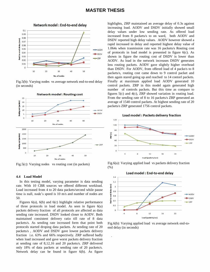
Figure 5(c) demonstrates routing cost offered by protocols.
From the figure, it is quite visible that routing load of ZRP is
much higher than of AODV and DSDV. As network became
fully dense the routing load of ZRP reached up to 1915
control packets per data packets. AODV and DSDV also
showed the same behavior. However, DSDV comparatively
gave low routing load and an increased of 3 to 4 control
packets are calculated as network size increased. AODV
seemed to approach to DSDV when network size was 20
nodes but just after this point the load raised and reached up
to 22 control packets. After the network size of 40 nodes we
saw a consistent performance of AODV.
MASTER THESIS
Fig.5(b): Varying nodes vs average network end-to-end delay
(in seconds)
Fig.5(c): Varying nodes vs routing cost (in packets)
4.4 Load Model In this testing model, varying parameter is data sending
rate. With 10 CBR sources we offered different workload.
Load increased from 4 to 20 data packets/second while pause
time is null, node’s speed is 10 m/s and number of nodes are
50.
Figures 6(a), 6(b) and 6(c) highlight relative performance
of three protocols in load model. As seen in figure 6(a)
packets delivery fraction of all protocols are affected as data
sending rate increased. DSDV looked closer to AODV. Both
maintained consistent delivery ratio till rate of 8 data
packets/s. As sending rate increased form that point both
protocols started droping data packets. At sending rate of 20
packets/s , AODV and DSDV gave lowest packets delivery
fraction i.e. 63% and 66% respectively. ZRP suffered badly
when load increased and gave worst packets delivery fraction
at sending rate of 8,12,16 and 20 packets/s. ZRP delivered
only 18% of data packets at sending rate of 20 packets/s.
Network delay can be found in figure 6(b). As figure
highlights, ZRP maintained an average delay of 0.3s against
increasing load. AODV and DSDV initially showed small
delay values under low sending rate. As offered load
increased from 8 packets/s to on ward, both AODV and
DSDV reported high delay values. AODV however showed a
rapid increased in delay and reported highest delay value of
1.064s when trasmission rate was 16 packets/s Routing cost
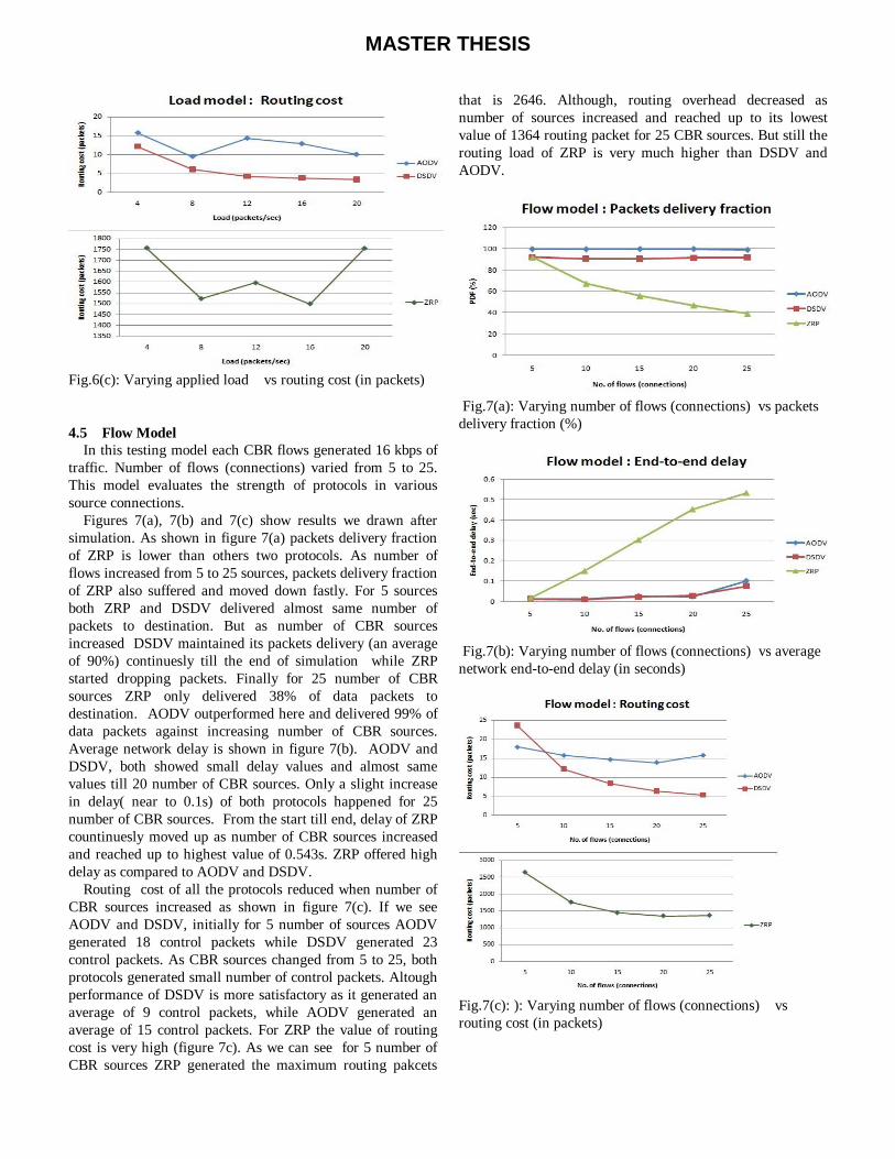
of protocols in load model is presented in figure 6(c). As
shown in figure the routing cost of DSDV is lower than
AODV. As load in the network increases DSDV generates
less routing packets. AODV gave slightly higher overhead
than DSDV. For AODV, from offered load of 4 packe/s to 8
packets/s, routing cost came down to 9 control packet and
then again stared going up and reached to 14 contorl packets.
Finally at maximum applied load AODV generated 10
control packets. ZRP in this model again generated high
number of controls packets. But this time as compare to
figures 5(c) and 4(c), ZRP showed variation in routing load.
From the sending rate of 8 to 16 packets/s ZRP generated an
average of 1540 control packets. At highest sending rate of 20
packets/s ZRP generated 1756 control packets.
Fig.6(a): Varying applied load vs packets delivery fraction
(%)
Fig.6(b): Varying applied load vs average network end-to-
end delay (in seconds)
.
MASTER THESIS
Fig.6(c): Varying applied load vs routing cost (in packets)
4.5 Flow Model
In this testing model each CBR flows generated 16 kbps of
traffic. Number of flows (connections) varied from 5 to 25.
This model evaluates the strength of protocols in various
source connections.
Figures 7(a), 7(b) and 7(c) show results we drawn after
simulation. As shown in figure 7(a) packets delivery fraction
of ZRP is lower than others two protocols. As number of
flows increased from 5 to 25 sources, packets delivery fraction
of ZRP also suffered and moved down fastly. For 5 sources
both ZRP and DSDV delivered almost same number of
packets to destination. But as number of CBR sources
increased DSDV maintained its packets delivery (an average
of 90%) continuesly till the end of simulation while ZRP
started dropping packets. Finally for 25 number of CBR
sources ZRP only delivered 38% of data packets to
destination. AODV outperformed here and delivered 99% of
data packets against increasing number of CBR sources.
Average network delay is shown in figure 7(b). AODV and
DSDV, both showed small delay values and almost same
values till 20 number of CBR sources. Only a slight increase
in delay( near to 0.1s) of both protocols happened for 25
number of CBR sources. From the start till end, delay of ZRP
countinuesly moved up as number of CBR sources increased
and reached up to highest value of 0.543s. ZRP offered high
delay as compared to AODV and DSDV.
Routing cost of all the protocols reduced when number of
CBR sources increased as shown in figure 7(c). If we see
AODV and DSDV, initially for 5 number of sources AODV
generated 18 control packets while DSDV generated 23
control packets. As CBR sources changed from 5 to 25, both
protocols generated small number of control packets. Altough
performance of DSDV is more satisfactory as it generated an
average of 9 control packets, while AODV generated an
average of 15 control packets. For ZRP the value of routing
cost is very high (figure 7c). As we can see for 5 number of
CBR sources ZRP generated the maximum routing pakcets
that is 2646. Although, routing overhead decreased as
number of sources increased and reached up to its lowest
value of 1364 routing packet for 25 CBR sources. But still the
routing load of ZRP is very much higher than DSDV and
AODV.
Fig.7(a): Varying number of flows (connections) vs packets
delivery fraction (%)
Fig.7(b): Varying number of flows (connections) vs average
network end-to-end delay (in seconds)
Fig.7(c): ): Varying number of flows (connections) vs
routing cost (in packets)
MASTER THESIS
5. COMPARISON AND DISCUSSION
After analyzing the simulation results in section 4, now it
will be understandable and helpful for us to compare and
discuss results, protocol’s behavior, their similarities and
differences. We basically, tested five different models. In
following paragraph we will compare the results of each
model separately (except pause time and speed models) with
respect to packets delivery fraction, routing cost and average
end-to- end delay.
Pause time and speed models both concern with node’s
movement and speed. Lower pause time means high node’s
random movement. While increasing node’s velocity with
respect to small pause time means higher node’s speed as
well as higher node’s movement. Figures 3(a), 3(b), 3(c) and
4(a), 4(b), 4(c) show results of both models obtained after
simulations. Results tells that, reactive routing is most
suitable in high mobile Ad Hoc networks than proactive and
hybrid routing. By increasing node’s movement and speed,
packets delivery fraction is not much affected for AODV but
for DSDV and ZRP packets delivery is not stable (figures 3(a)
and 4(a)). From pause time 0s to 400s (high to low node’s
movement) and speed from 10 m/s to 50 m/s (low to high
mobility), only AODV provides an average of 98% of packets
delivery for all different levels. While packets delivery
fraction of DSDV and ZRP increased as nodes movement and
speed decreased (figures 3(a) and 4(a)). The best performance
of AODV is because of its on demand nature. Only when
nodes want to send data connection is established. This helps
AODV to actively find routes in high mobility when routes
break frequently. Although this fast routes discovery of
AODV leads to better delivery fraction but increases routing
overhead. As compared to DSDV (figure 3(c) and 4(c)),
routing overhead of AODV is higher in high mobility and
increased as speed increased. Routing overhead of proactive
protocol (DSDV) is comparatively low or stable than AODV.
This is because of periodic updates of DSDV. But always
depending on these periodic update’s information, chance to
select stale route (in high mobility) increases that causes
packets to be dropped. As we can see from figures 3(a) and
4(a), DSDV gives bit low delivery ratio (nearly about 90%) at
high mobility. As mobility increases packets started dropping
(figure 4(a)). But as network became static DSDV delivery
fraction reached up to AODV (figure 3(a)). In both models,
average end to end delay of AODV and DSDV was almost
same (figures 3(b) and 3(c)). There isn’t any noticeable
difference. But for ZRP there are high delay values especially
at high mobility. Performance of ZRP is found average in
speed and pause time models. ZRP is not a pure proactive
neither a pure reactive protocol, rather it uses both routing
techniques. The only attribute on which the performance of
ZRP depends is its zone radius. Some studies have been
conducted to evaluate the performance of ZRP under different
zones radius. As we know, in Ad Hoc networks, network
parameters change with respect to time and it is very difficult
to have exact knowledge of network size, nodes density and
node’s velocity therefore adjusting radius parameter in reality
is a complicated task. From figure 3(c) and 4(c), it is quite
obvious that control overhead of ZRP is relatively higher than
AODV and DSDV. This is because of two reasons. Firstly,
increase in IARP (proactive) periodic routing updates and
secondly, IERP (reactive) frequently route failures. High
nodes movement not only causes frequently routes failure but
continuous change in neighbors requires every node to update
its zone information which significantly doubles the amount
of control traffic generated by IARP. Another possible reason
in case of ZRP which causes high routing overhead is
overlapping of zones. This overlapping of zones increases
number of query packets of IERP as well as periodic updates
of IARP. From low to high nodes movement, packets delivery
fraction of ZRP suffer as shown in figure 3(a) and 4(a),
secondly high delay values as compared to AODV and DSDV
(figures 3(b) and 4(b)). The possible explanation is selecting
wrong path and taking more time to compute path from
source to destination. Because of delay in path computing in
high mobility data packets wait in send buffer for a long time
and start dropping when buffer overflows. From this
discussion we can simply conclude that reactive routing
outperformed and second best performance is given by
proactive routing. However, hybrid routing is not favorable in
highly dynamic topology. We will give a detail conclusion at
the end of this report and provide some issues related to
hybrid routing.
In network model number of nodes varies from 10 to 50
and simulation results are presented in figures 5(a), 5(b) and
5(c). When network becomes dense, a general observation is
increase in routing overhead. As from figure 5(c), we can see
a linear growth in routing traffic of AODV, DSDV and ZRP.
However, routing overhead of ZRP is very high. As the nodes
increases more routes become available to destinations. Since
AODV is reactive protocol and reacts very fast in order to
compute routes. Because it uses one active route therefore we
can see best delivery fraction of AODV (figure 5(a)). But
establishing routes on demand increases the flooding of
RREQ and RREP queries. DSDV on the other hand gives low
routing overhead than AODV but packets delivery ratio is
less than AODV and ZRP. When new routes become
available more frequently and dependence of DSDV on the
routes in routing table, increases chance to select the stale and
broken routes hence packets drop. When we compare the
performance of ZRP with others two protocols in terms of
packets delivery fraction, ZRP secures second best position
(figure 5(a)). From network size of 10 to 40 nodes, ZRP
delivers an average of 95% of data packets. Although when
network become full dense the packets delivery fraction of
ZRP falls down to 69 %. We will discuss the possible reason
of this downfall latter because in general, the delivery fraction
should have increased since ZRP is protocol that targets large
network. For ZRP as discussed earlier the most important
thing is zone radius. In our simulation environment the zone
radius is taken 2 nodes distance. Figure 5(c) show the routing
MASTER THESIS
load of ZRP and a significant growth in routing load as
network become dense. With zone radius value 2 and less
number of nodes most of traffic is generated by IARP
(proactive routing) but as the nodes increases (constant zone
radius value 2) he burden on IERP (reactive routing)
increases hence more control traffic is generated by IERP.
Simulation performance in [11] shows network size and no.
of neighbors of node are main factors which effect the
performance of ZRP. In this situation the only configurable
parameter to control the routing traffic is adjusting the zone
radius. Small zone radius with increasing network size
increases reactive control traffic as well as local periodic
updates of proactive routing. A large zone radius can
significantly decreases the amount of routing traffic in large
networks. The packets delivery fraction down fall of ZRP
from nodes 40 to 50 is because of same reason as described
earlier. More routing packets show ZRP is trying to converge
and finding routes to destination. Moreover the possibility of
zones overlapping can’t also be denied. All of these issues
collectively cause for ZRP to drop packets and increase in
average end-to- end delay as shown in figure 5(b). From this
comparative discussion we simply conclude that AODV is
favorable routing protocol in large networks. ZRP can be used
more effectively in large networks only by configuring its
zone radius. DSDV seems not to be good in terms of delivery
fraction as far as our simulation results are concerns.
In order to check the affects of sending rates we applied
different work load in load model. Results are presented in
figures 6(a), 6(b) and 6 (c). We increased sending rates from
4 packets/sec to 20 packets/sec (i.e. 4, 8, 12, 16 and 20
packets/s). Figure 6(a) shows packets delivery fraction of all
three protocols. At low sending rate, from 4 to 8 packets/sec
both AODV and DSDV gave good delivery fraction (average
of 98% and 90% respectively). However, DSDV performed
bit low than AODV. ZRP, on the other hand performed very
poorly. As described in pause time and speed model, both
DSDV and ZRP cannot easily adopt high mobility. Therefore
initially both protocols suffered from high nodes movement
(pause time null) and speed (10 m/s). On demand routing
(AODV) acts well in dynamically changing topology, hence it
gives almost 100% packets delivery at low sending rate. As
sending rate increases from 8 packets/sec, all protocols
performance degraded (figure 6(a)). In this situation protocols
are not only dealing with workload but also dealing with
dynamically changing topology. But the main reason for
dropping such a large number of packets at high sending rate
is because of congestion. When the sending rate of source
node is high then its neighbors become congested very soon.
At sending rate of 16 and 20 packets/sec, when collective
network bandwidth utilization reaches up to 1 MB, it is quite
meaningful that most of the packets are being dropped by
forwarding nodes. Since the nodes in Ad Hoc have limited
resources like storage and queue sizes. When congestion
occurs it becomes difficult for nodes to keep the packets for
long time hence queue overflows and drops packets. Beside
limited node’s resources which are same for every protocol in
simulation environment, further difference in performance is
made by routing techniques and congestion control
mechanisms. AODV uses binary exponential backoff to
control congestion but it doesn’t seem to be affective here. In
addition, AODV has only actives routes therefore in the case
of congestion route recovery mechanism of AODV can use
the active route of neighboring nodes. Therefore AODV gives
slightly better delivery fraction than DSDV. DSDV shows
some similarity in delivery fraction with AODV (figure 6(a)).
Comparing with AODV delivery ratio, the DSDV competes
because of availability of alternatives routes, however, DSDV
can’t prepare itself to the congestion. Although, in ZRP, flat
routing reduces congestion but at high data rate, high
mobility, big network size with chances of zones overlapping,
the border nodes can become the traffic’s target and resulting
in network congestion. Because nodes in single zone are
prohibited from communicating to other zone’s nodes
directly. This situation of congestion can also be observed
from figure 6(b), when average end to end delay of network
increases rapidly for AODV and DSDV. That means data
packets are taking more time to reach to destination.
However, ZRP offered comparatively low network delay but it
also delivered small no. of data packets. Similarly routing
load is decreasing when sending rate is increasing (figure
6(c)). AODV routing overhead is higher than DSDV, this is
because of its periodic Helo messages to maintain active
roués, while DSDV makes use of alternative routes that is
why its routing overhead is lower than AODV. For ZRP the
routing overhead is too high and we have already mentioned
the reasons in previous discussions.
Flow model simulation results are presented in figures 7(a),
7(b) and 7(c). When numbers of flows (connections)
increases, AODV has better delivery fraction than DSDV and
ZRP. Because of on-demand nature AODV always choose
fresh routes therefore probability of dropping packets is very
low and large numbers of packets are delivered to destination
(figure 7(a)). Always choosing active routes requires AODV
to initiate route discovery process most frequently therefore
routing overhead of AODV is higher than DSDV (figure
7(c)). For DSDV we received an average of 91% of delivery
fraction. DSDV performance is bit lower than AODV nearly
8%. On the other hand, routing load of DSDV is better than
AODV (figure 7(c)). This low routing load of DSDV is
because of local periodic messages which keep routing table
update. In average end to end delay, there is similarity
between AODV and DSDV till 20 flows (figure 7(b)). In
between 20 to 25 flows, there is a very small ignorable rise in
the delay offered by AODV. In the stressful condition with
increasing number of flows, ZRP performance found to be
very poor when compare with pure reactive (AODV) and pure
proactive (DSDV) protocols. We were not expecting such a
bad performance from ZRP in flow model. In order to find the
reasons we observed the NAM animator of NS2 for ZRP
simulation. Finally we came to the conclusion that, there are
MASTER THESIS
many factors which collectively degrading the performance of
ZRP. Firstly, nodes positions may cause several zones to
overlap because we have network of 50 nodes. This zones
overlapping significantly increase IARP control traffic for
keeping the zones information up to date. Secondly, as the
numbers of flows are increasing that means more connections
are needed to be established with in zones and outside the
zones. Thirdly, when zones overlap numbers of connections
increase and every source connection is sending data at a rate
of 16kbps, since there is possibility that many sending nodes
are targeting a single border node and because of limited
storage resources of nodes the delivery fraction of network
falls down. This situation also leads the network to become
fully congested and packets may collide hence overall
performance decreased as shown in figure 7(a), 7(b) and 7(c).
6. CONCLUSION
In this thesis we compared the performance of three
routing protocols (AODV,DSDV and ZRP) in five different
models in NS2. Main performance metrics are packets
delivery ratio, average end-to-end delay and routing load. In
all the models AODV outperformed in term of packets
delivery ratio. In speed and pause time model, where routes
breaking ratio was very high, only AODV maintained high
delivery ratio. Since AODV is on demand routing protocol
therefore always selecting fresh and active route made it
possible to deliver large number of data packets. But this fast
route discovery of AODV caused more routing packets in the
network, therefore, as compared to DSDV, its routing
overhead is high and also showed slightly high delay. ZRP in
speed and pause time model showed average performance.
Increasing speed not only caused to drop large number of data
packets but also very high routing overhead and delay. In
network model where the network size was increasing, ZRP
performed very well. Although its routing overhead was
higher than DSDV and AODV but average network delay and
packets delivery ratio are found to be very good. Since ZRP
targets large networks so it can be used more effectively by
adjusting its optimal zone radius. In load model where
workload was increasing. Performance of all the protocols
degraded. It seemed that protocols are not capable to react
well when sending rate is high. Lack of affective congestion
control mechanism, limited node’s resources such as storage,
bandwidth and transmission range make it very difficult for
protocols to handle high data rate. In flow model, AODV is
not much affected and DSDV also gave consistent packets
delivery. Average end-to-end delay of both protocols are also
very low. But increasing connections caused AODV to gave
slightly high routing overhead than DSDV. ZRP seemed very
sensitive in flow model. Increasing no of connections
decreased the packets delivery and gave relatively high delay
and routing load.
The bottom line is, AODV performance was best while
DSDV secured second best position. ZRP gave an average
performance except in network model. For ZRP there are
some concerns. ZRP is framework of three routing protocols
i.e. IARP, IERP and BRP and the effectiveness of these three
routing protocols mainly depend on node’s radius. Selecting
an optimal zone radius can reduce routing traffic and improve
ZRP performance. But for this purpose it is necessary to have
understanding of how network is affected by different factors.
For every network there will be different zone radius
according to its structure. In addition, several others factors
collectively determine ZRP performance. For instance, cache
mechanism of ZRP, where no longer used routes are kept for
long time and under sturated situation deletion of routes takes
place prematurely. It results in high end-to-end delay and
routing overhead. Improving cache mechanism by associating
information priority with latest access time to every route in
routing table reduced end-to-end delay and routing overhed as
described in [13]. In place of IARP and IERP different
proactive and reactive approaches can be used. As duscussed
in [14], selection of link state instead of distance vector with
in zones results in evenly distribution of traffic. Query node
plays a vital role. Selection of precise query node (good
battery and processing power) will always improve ZRP
performance.
7. ACKNOWLEDGEMENT
I would like to thanks to the supervisor of this thesis work Dr.
Stanislav Belenki for his support and guidance and best
regards for University West faculty.
MASTER THESIS
REFERENCES
[1] Toh,C.-K.;Delwar, M.; Allen,D.;"Evaluating the communication
performance of an ad hoc wireless network," Wireless Communications, IEEE Transactions on , vol.1, no.3, pp.402-414, Jul 2002
[2] Al Turki, R.; Mehmood, R.; , "Multimedia Ad oc
Networks: Performance Analysis," omputer Modeling and Simulation, 2008. EMS '08. Second UKSIM European Symposium on , vol., no., pp.561-566, 8-10 Sept. 2008
[3] Perkins, D.D.; Hughes, H.D.; Owen, C.B.; , "Factors affecting the
performance of ad hoc networks," Communications, 2002. ICC 2002. IEEE International Conference on , vol.4, no., pp. 2048- 2052 vol.4, 2002
[4] Geetha, Gopinath.“Performance Comparison of Mobile Ad-Hoc Network
Routing Protocols”. 11 Nov.2007. Web. 04 March 2010. <http://citeseerx.ist.psu.edu/viewdoc/download?doi=10.1.1.126.9426&rep=rep1&type=pdf>
[5] C. E. Perkins and E. M. Royer. Ad Hoc On Demand Distance Vector
(AODV) Routing. IETF lnternet Draft, draft-ietf-manet-aodv-O~.txt, November 1998. (Work in Progress).
[6] Chowdhury, M.U.;Perera, D.; Pham,t.;"A performance comparison of
three wireless multi hop ad-hoc network routing protocols when streaming mpeg4 traffic," Multi topic conference, 2004. proceedings of inmic 2004. 8th international , vol., no., pp. 516- 521, 24-26 Dec. 2004
[7] Perkins, C. E. and Bhagwat, P. 1994. Highly dynamic Destination-
Sequenced Distance-Vector routing (DSDV) for mobile computers. SIGCOMM Comput. Commun. Rev. 24, 4 (Oct. 1994), 234-244
[8] Ahmed, M.; Yousef, S.; , "Self-configurable zone routing
protocol attributes," Industrial Electronics, 2008. ISIE 2008. IEEE International Symposium on , vol., no., pp.2119-2124, June 30 2008-July 2 2008
[9] Pearlman, M.R. and Hass, Z.J., Determining the optimal configuration for
the zone routing protocol. IEEE Journal on Selected Areas in Communications. v17 i8. 1395-1414.
[10] Patel, B.; Srivastava, S.; , "Performance analysis of zone
routing protocols in Mobile Ad Hoc Networks," Communications (NCC), 2010 National Conference on, vol.,pp.1-5, 29-31 Jan. 2010
[11] Network Simulator 2, www.isi.edu/nsnam/ns, 2010. [12] Nor. S, Azizol A, Ahmed F “Performance Evaluation of AODV, DSDV
& DSR Routing Protocol in Grid Environment” July 2009. Web. 09 July
2010. <http://paper.ijcsns.org/07_book/200907/20090737.pdf> [13] Hao-jun Li; Fei-yue Qiu; Yu-jun Liu; , "Research on Mechanism
Optimization of ZRP Cache Information Processing in Mobile Ad Hoc Network," Wireless Communications, Networking and Mobile Computing, 2007. WiCom 2007. International Conference on , vol., no., pp.1593-1596, 21-25 Sept. 2007
[14] Sulaiman, T.H.; Al-Raweshidy, H.S.; , "Centralised Link-State Routing in
ZRP," Personal, Indoor and Mobile Radio Communications, 2006 IEEE
17th International Symposium on , vol., no., pp.1-5, 11-14 Sept. 2006
MASTER THESIS
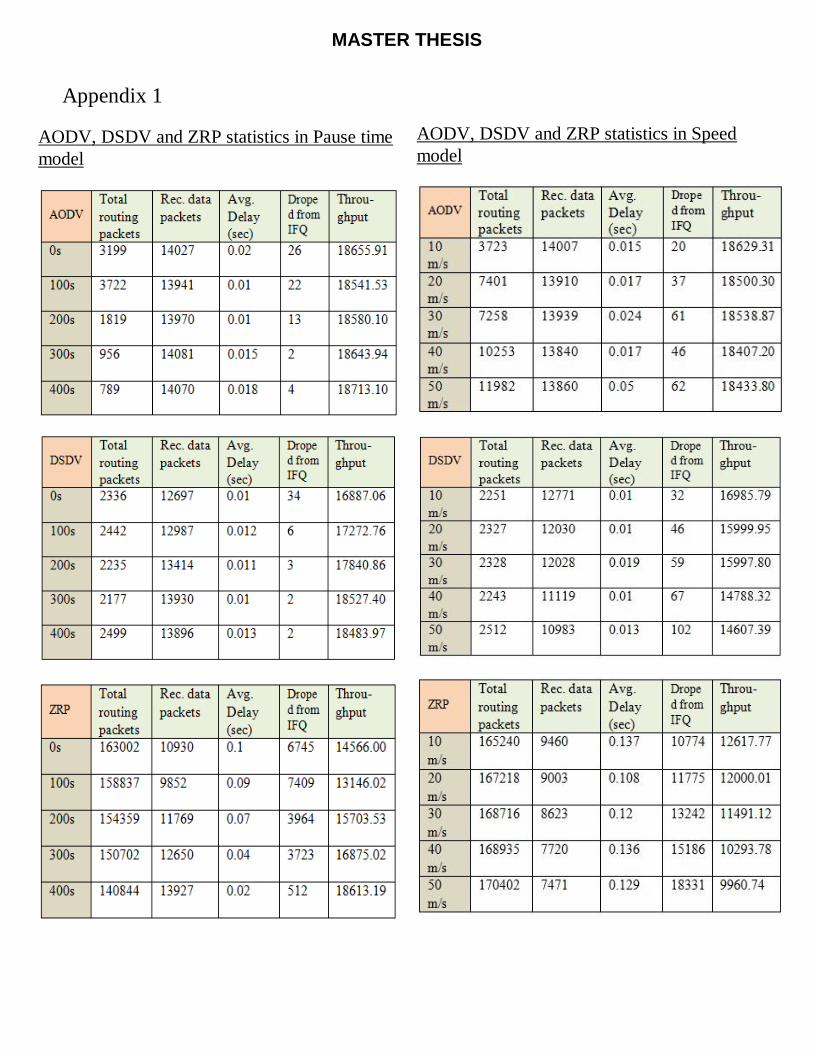
Appendix 1
AODV, DSDV and ZRP statistics in Pause time
model
AODV, DSDV and ZRP statistics in Speed
model
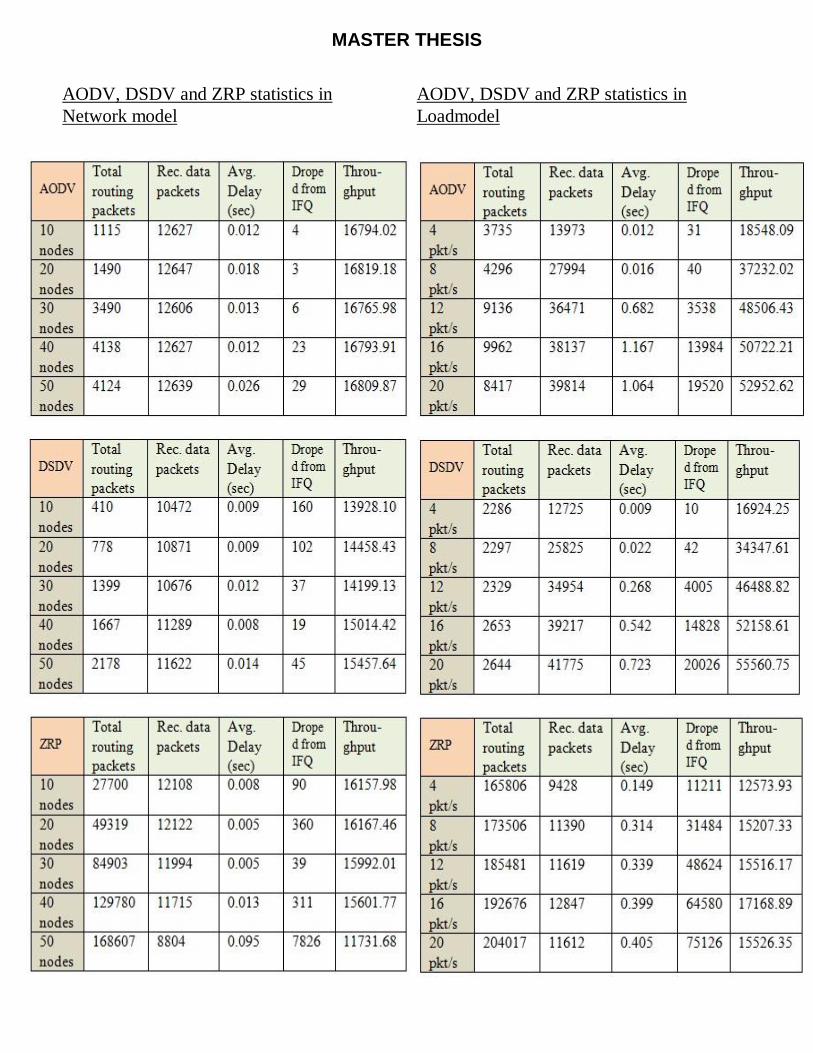
MASTER THESIS
AODV, DSDV and ZRP statistics in
Network model
AODV, DSDV and ZRP statistics in
Loadmodel
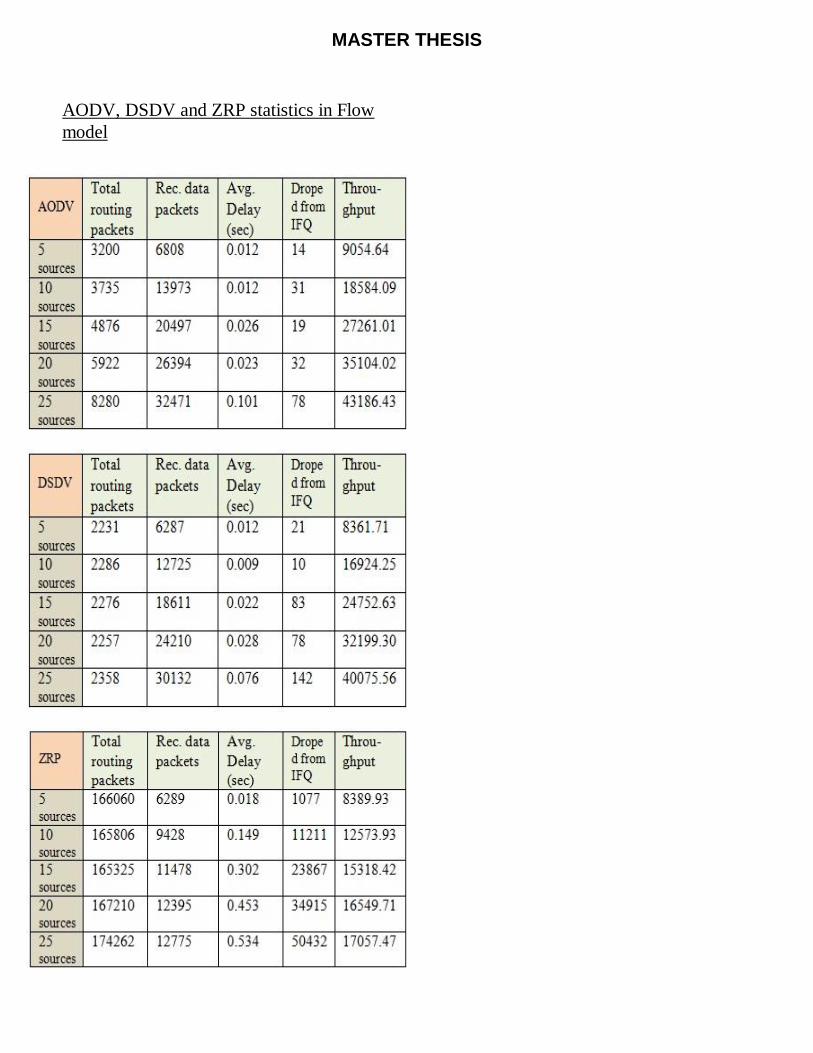
MASTER THESIS
AODV, DSDV and ZRP statistics in Flow
model
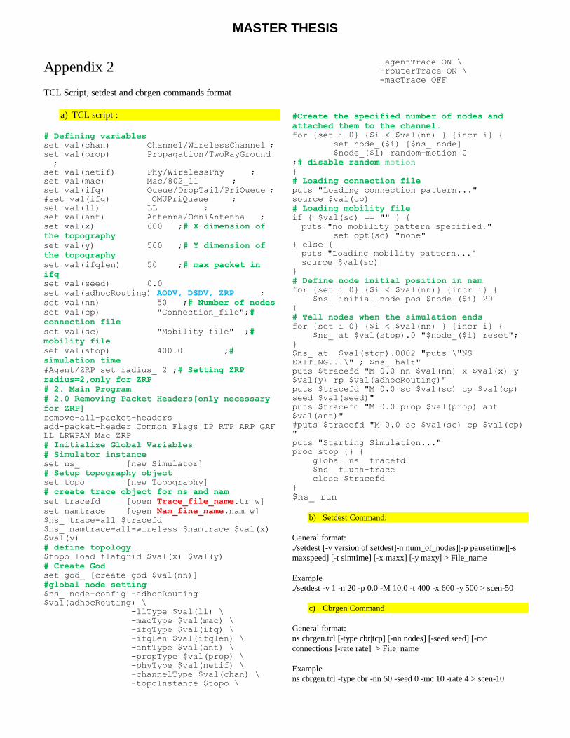
MASTER THESIS
Appendix 2
TCL Script, setdest and cbrgen commands format
a) TCL script :
# Defining variables
set val(chan) Channel/WirelessChannel ;
set val(prop) Propagation/TwoRayGround
;
set val(netif) Phy/WirelessPhy ;
set val(mac) Mac/802_11 ;
set val(ifq) Queue/DropTail/PriQueue ;
#set val(ifq) CMUPriQueue ;
set val(ll) LL ;
set val(ant) Antenna/OmniAntenna ;
set val(x) 600 ;# X dimension of
the topography
set val(y) 500 ;# Y dimension of
the topography
set val(ifqlen) 50 ;# max packet in
ifq
set val(seed) 0.0
set val(adhocRouting) AODV, DSDV, ZRP ;
set val(nn) 50 ;# Number of nodes
set val(cp) "Connection_file";#
connection file
set val(sc) "Mobility_file" ;#
mobility file
set val(stop) 400.0 ;#
simulation time
#Agent/ZRP set radius_ 2 ;# Setting ZRP
radius=2,only for ZRP
# 2. Main Program
# 2.0 Removing Packet Headers[only necessary
for ZRP]
remove-all-packet-headers
add-packet-header Common Flags IP RTP ARP GAF
LL LRWPAN Mac ZRP
# Initialize Global Variables
# Simulator instance
set ns_ [new Simulator]
# Setup topography object
set topo [new Topography]
# create trace object for ns and nam
set tracefd [open Trace_file_name.tr w]
set namtrace [open Nam_fine_name.nam w]
$ns_ trace-all $tracefd
$ns_ namtrace-all-wireless $namtrace $val(x)
$val(y)
# define topology
$topo load_flatgrid $val(x) $val(y)
# Create God
set god_ [create-god $val(nn)]
#global node setting
$ns_ node-config -adhocRouting
$val(adhocRouting) \
-llType $val(ll) \
-macType $val(mac) \
-ifqType $val(ifq) \
-ifqLen $val(ifqlen) \
-antType $val(ant) \
-propType $val(prop) \
-phyType $val(netif) \
-channelType $val(chan) \
-topoInstance $topo \
-agentTrace ON \
-routerTrace ON \
-macTrace OFF
#Create the specified number of nodes and
attached them to the channel.
for {set i 0} {$i < $val(nn) } {incr i} {
set node_($i) [$ns_ node]
$node_($i) random-motion 0
;# disable random motion
}
# Loading connection file
puts "Loading connection pattern..."
source $val(cp)
# Loading mobility file
if { $val(sc) == "" } {
puts "no mobility pattern specified."
set opt(sc) "none"
} else {
puts "Loading mobility pattern..."
source $val(sc)
}
# Define node initial position in nam
for {set i 0} {$i < $val(nn)} {incr i} {
$ns_ initial_node_pos $node_($i) 20
}
# Tell nodes when the simulation ends
for {set i 0} {$i < $val(nn) } {incr i} {
$ns_ at $val(stop).0 "$node_($i) reset";
}
$ns_ at $val(stop).0002 "puts \"NS
EXITING...\" ; $ns_ halt"
puts $tracefd "M 0.0 nn $val(nn) x $val(x) y
$val(y) rp $val(adhocRouting)"
puts $tracefd "M 0.0 sc $val(sc) cp $val(cp)
seed $val(seed)"
puts $tracefd "M 0.0 prop $val(prop) ant
$val(ant)"
#puts $tracefd "M 0.0 sc $val(sc) cp $val(cp)
"
puts "Starting Simulation..."
proc stop {} {
global ns_ tracefd
$ns_ flush-trace
close $tracefd
}
$ns_ run
b) Setdest Command:
General format:
./setdest [-v version of setdest]-n num_of_nodes][-p pausetime][-s
maxspeed] [-t simtime] [-x maxx] [-y maxy] > File_name
Example
./setdest -v 1 -n 20 -p 0.0 -M 10.0 -t 400 -x 600 -y 500 > scen-50
c) Cbrgen Command
General format:
ns cbrgen.tcl [-type cbr|tcp] [-nn nodes] [-seed seed] [-mc
connections][-rate rate] > File_name
Example
ns cbrgen.tcl -type cbr -nn 50 -seed 0 -mc 10 -rate 4 > scen-10
MASTER THESIS
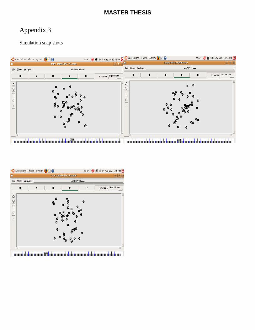
Appendix 3
Simulation snap shots