Marking to Market, Trading Activity andMutual Fund Performance
Sugato Bhattacharyya1
University of Michigan
Vikram Nanda
University of Michigan
(This version: March 2005)
1The paper is currently in revision and, hence, incomplete. It is a subsantially revised versionof another paper �rst circulated in September 1999. We wish to thank seminar participants atthe following institutions for their comments on earlier versions of this paper: Australian NationalUniversity, University of British Columbia, Duke University, Indiana University, London BusinessSchool, Melbourne University, University of Michigan, University of Minnesota, New York University,Princeton University, Sydney University, Tulane Univrsity, HEC at Paris and the University ofAmsterdam. All errors are the responsibility of the authors.
1
Abstract:
Marking to Market, Trading Activity and Mutual Fund Performance
This paper analyzes the portfolio decisions of a mutual fund manager who cares
about her short-term performance as measured by the Net Asset Value of her fund. We
show that such preferences lead to trading even without favorable information in order
to enhance short-term rewards. We show that information about the fund�s portfolio
position is valuable and that closed-end funds may trade at discounts or premia to
measured asset values. Patterns in closed-end fund premia are easily explained with
the help of the paper�s model.
2

1 Introduction
Mutual funds play an increasingly important role in �nancial markets around the
world. According to the Investment Company Institute2, the number of mutual funds
worldwide has increased from 50,835 in 1998 to 54,015 in 20043. This growth in num-
bers has been accompanied by a remarkable rise in the the value of assets held by
mutual funds: from $9.34 trillion in 1998 to $13.96 trillion at the end of 2003. Over
the last twenty years, mutual funds have been a prime investment vehicle for individ-
ual investors. In fact, for most this time period, purchases of equity by households
through mutual funds have been positive every year while net purchases made outside
mutual funds have mostly been negative. Consequently, there has been a continued
shift in ownership of equities from individual ownership to ownership through mutual
funds. At end-2003, assets of U.S. equity mutual funds stood at $3.68 trillion, while
total mutual fund assets, including money market funds, bond funds and hybrid funds
stood at $7.41 trillion. The total amount of �nancial assets owned through mutual
funds is comparable to the total loans and investments of all commercial banks in the
United States and total equity holdings by mutual funds account for about 20% of
all U. S. equities by value. This increasing trend of indirect holdings through mutual
funds is not just a characteristic of domestic markets, but also has been a feature
of most international markets throughout the 1990s. In fact, a large portion of the
divestment of government owned asset by countries restructuring their economies in
Eastern Europe and Asia, has been undertaken with the help of new or existing
mutual funds.
It is clear, then, mutual funds are important investment vehicles and, thus, merit
the attention of researchers. While there has been a signi�cant body of work built up
during the last three decades regarding the performance of mutual funds4, there seems
to have been a paucity of theoretical models investigating the decision criteria used
by mutual fund managers. Consequently, while in the area of corporate �nance, the
2See the Investment Company Institute�s publication Mutual Fund Factbook for data on trendsin the mutual fund industry. Data reported here are from the 2004 issue (44th edition) .
3The corresponding numbers for the U.S. are 7,314 and 8,126 respectively.4For an overall view of the empirical facts and trends, see Sirri and Tufano (1993).
3

paradigm of agency costs has been well explored and applied to generate implications
for corporate managers, there does not exist a cogent body of work which attempts to
apply similar insights to world of mutual funds5. The literature that exists to date has
concentrated on the structure of fees for mutual fund managers (Chordia (1996)), the
structure of mutual funds and optimal managerial strategies (Nanda, Narayanan and
Warther (1998), Nanda and Singh (1999)) and the e¤ect of performance measures on
the portfolio composition undertaken by fund managers (see Huddart (1998)). In this
paper, we focus, instead, on the incentives of fund managers who are rewarded based
on their asset holdings, to deviate from the interests of long-term value maximization.
The basic model examines the incentive of informed fund managers to trade ex-
cessively in the direction of their portfolio holdings. Such trading is an attempt at
bolstering the value of the existing portfolio even though this may detract from maxi-
mizing long-term pro�ts. We demonstrate that managers�incentives to engage in such
trade goes up with the size of their holdings. While such trading may very well be
anticipated and accounted for in the pricing of traded securities, we show that, nev-
ertheless, there will be incentives to engage in such trade. In face of such anticipation
by price setters in the �nancial markets, it is costly, in terms of short-term portfolio
values, not to engage in such trade. We show that this incentive is strong enough to
generate trade even in the absence of liquidity traders who care only about execution
and not pro�tability. Thus, we are able to provide some justi�cation to the thesis
that greater institutional holdings generate higher trading activity in markets. Our
trading results rely only on the agency problems between managers and long-term
investors and we do not need to invoke diversi�cation as a motive for trade.
We extend our analysis to ask whether fund managers should disclose their historic
portfolio holdings to reduce the impact of inventory uncertainty on their portfolio
values. We establish that, even though long-term investors prefer such disclosure,
the manager (and investors who need to liquidate in the short-term) do not favor
such disclosure. We show that this result arises because increases in Net Asset Value
(NAV) in the short-run are aided by this lack of disclosure, which makes it hard for
market participants to distinguish between price moves that are caused by a change
5Prominent exceptions are Dow and Gorton (1997) and Berk and Green (2004).
4

in fundamentals and those caused by order imbalances. Finally, we demonstrate that
having access to the outstanding portfolio composition of a mutual fund has value to
an investor who is ready to trade strategically on that information. As a result, the
manager has even greater incentive to withhold such information.
While much of our analysis is performed in the context of no-load, open-end
mutual funds, our model also has implications for the closed-end fund puzzle. A
long-standing anomaly in the �nance literature has been the persistent downward
bias of market values of closed-end funds from their Net Asset Values. There exists
an extensive literature on the subject and a wide variety of proposed solutions to the
puzzle. Some of these explanations concentrate on tax and illiquidity factors to argue
for an upward bias in reported NAVs, while others focus on market sentiment to argue
for variable biases in the market value of closed-end funds6. Our model generates an
upward bias in the short-run NAV due to market�s inability to distinguish between
price moves caused by fundamental information and by non-informational trading by
mutual fund managers. In this setting, we show that closed-end funds may very well
sell at a premium or at a discount to their NAVs. We derive conditions under which
either situation prevails. In our model, it is entirely reasonable for closed-end funds
to start o¤ at a premium to their NAVs and to then drift downwards with time. Our
model generates several other empirically testable propositions.
In terms of its motivation, our model is most closely related to work by Dow and
Gorton (1997) who also look at the incentives of mutual fund managers to engage in
excessive trading. In their model, excessive trading results from an attempt by an
agent to convince the principal that she possesses private information about security
values since, otherwise, her actions could not be distinguished from those of unin-
formed managers. In contrast, our model does not generate trading to induce such
separation in types: Excessive trading results from an attempt to in�uence prices,
whether successful or not. More recently, Berk and Green (2004) present an analysis
of mutual fund trading activity where managerial talent has decreasing returns to
scale. They calibrate their model to show that it can explain several stylized facts
6See Dimson and Minio-Kozerski (1999) for a recent survey of the literature on closed-end funds.
5
about pro�tability of mutual funds and its relationship to �ows into and out of funds7.
Their analysis does not address the market impact issues directly, although decreasing
returns to scale is consistent with this factor.
Finally, Carhart et al (2002) provide empirical support for several of our results.
They provide evidence that fund managers in�ate quarter-end portfolio prices with
last-minute purchase of stocks already held and that there is a surge in trading in
the last minutes of a quarter. They o¤er a couple of hypotheses as to why such an
empricial pattern emerges and conclude that it is likely that such behavior is caused
by managerial compensation considerations. Our model, indeed, establishes formally
that such patterns would be expected when managerial compensation considerations
are important.
The paper proceeds as follows. In Section 2, we consider the case of the manager
of an open-end mutual fund who ignores the impact of her own trading strategy on
market parameters and estabish the basic result of excessive trading. In Section 3, we
consider the more general case of market participants anticipating the impact of their
trading strategies on market parameters. In Section 4, we examine the incentives
of various parties to disclose information about portfolio holdings. In Section 5, we
extend our analysis to the case of closed-end funds, while implications and extensions
are presented in Section 6. Section 7 concludes.
2 The Base Model
For the base model, we consider the case of a single open-end, no-load, mutual fund
that trades in two securities: a risk-free asset and a risky asset. The risky asset is
traded in a batched order market a la Kyle (1985): all market orders and submitted
simultaneously and a market-clearing position is taken by a market maker. There are
three dates. At date 0, there are no asymmetries in information about the prospects
for the risky security and its per-unit price is given by P0. The mutual fund has an
inventory of z units of the risky security and I0 � zP0 invested in the risk-less asset.7See also Edelen (1999) for an empirical examination of related issues.
6

Sometime during the �rst period, the fund manager receives private information
about the payo¤ of the risky security and decides on the market order to place with
the market maker. At date 1, the market maker batches all market orders received
during the period and clears the market for the risky security, thus establishing a
trading price. At the end of trading on date 1, the fund announces its Net Asset
Value (NAV), computed using the market prices of its holdings. At date 2, the payo¤
to the risky security is realized. For simplicity, we assume that there is no other
new information or trading during the second period. All players are assumed to be
risk-neutral and the risk-free rate is normalized to be zero.
The mutual fund manager is assumed to have perfect information about the risky
security�s payo¤. We denote this payo¤ by the random variable ~v and the manager�s
market order by ~x(v). In the base model, we do not specify the trading strategies
of other traders but take it as given that they have either information or liquidity
needs to engage in trading. The market maker gets to observe the aggregate order
�ow, ~y, and sets a price at which the market clears. For now, we assume that the
market maker�s price setting process results in a linear price schedule of the form
P1 = P0 + �y, where � > 0 is a parameter that re�ects the market depth. The slope
of the price schedule could arise, for present purposes, due to either the anticipated
presence of other informed traders or due to inventory-theoretic considerations that
a¤ect the market maker�s pricing strategy8. We assume that the mutual fund manager
takes the value of � as given and that the competition between market makers ensures
that market-clearing prices are semi-strong form e¢ cient. Note that this implies that
E(P1) = P0 and that E(y) = 0.
In order to analyze the optimal choice of the market order placed by the mutual
fund manager, we need to �rst specify an objective function for the manager. We
assume that the mutual fund manager places a weight of on the NAV of the fund
at date 1 and a weight of (1 � ) on the liquidation value of the fund, where 0 < < 1. This objective function is motivated by the commonly observed compensation
8Glosten and Milgrom (1985), Easley and O�Hara (1987), among others, analyze models ofmarket-making where price responds to order size due to adverse selection considerations. Ho andStoll (1981) is an example where the responsiveness of price to volume is due to inventory-theoreticconsiderations.
7

functions prevalent in the mutual fund industry, in which a substantial portion of
managerial fees are in the form of a set percentage of (the current market value of)
total assets under management. In addition, Sirri and Tufano (1998) and Chevalier
and Ellison (1997) have shown that fund �ows in to and out of mutual funds are
strongly related to lagge measures of performance. Thus, it stands to reason that
fund managers would have strong incentives to care about both short and long term
performance in making trading decisions9.The �ow of funds argument can also be
formalized without considering investor response to current performance. Suppose,
for example, that the fund manager acts in the interest of ex ante identical investors
who have claims on the fund. With some probability, each investor su¤ers a liquidity
shock at time 1, which leads to the redemption of his entire claim at that point in
time10. Given the open-end nature of the fund, redemptions are computed using the
NAV �gure at date 1. The remaining investors stay invested in the fund up until date
2 and realize liquidation proceeds when the risky asset pays o¤. In this environment,
it is ex ante optimal for the manager to be provided with incentives to maximize an
objective function that involves both the liquidation value of the fund and its NAV
at date 111.
It is also worth noting that this form of an objective function has been used
in the context of agency considerations which would, clearly, apply in the context
of decisions by a professional fund manager. For example, Miller and Rock (1985)
consider such an objective function in the context of a corporate manager making a
decision on dividend and investment policies. It is relatively straightforward to show
that an attempt to elicit optimal actions on the part of a manager in a situation
where either managerial tenure is stochastic or investor response to performance is
rational would also involve incentive schemes which reward both short and long-term
performance . Finally, managerial concern about near-term performance also arise
when they borrow money to �nance their activities: borrowers�concerns about being
9The linearity feature is not essential for our results but allows for closed form solutions.10This argument is similar to the one found in many banking models. See, for example, Diamond
and Dybvig (1986).11Nanda and Singh (1999) discuss the e¤ect of early redemption on the incentives of other investors
to remain with the fund. For the sake of simplicity, we do not explicitly account for the cost of earlyredemption on investors who do not redeem early.
8

repaid also makes a manager care about short-term performance. In recent times,
perhaps the most dramatic illustration of this principle was seen in the case of Long
Term Capital Management (LTCM). It has been argued by several observers that the
trading strategy pursued by LTCM could reasonably have been expected to result in
pro�ts over the long run. However, unanticipated short-termmovements that widened
historical credit spreads made LTCM�s portfolio lose a signi�cant proportion of its
value and resulted in its inability to sustain its leverage.
The structure laid out above is su¢ cient for us to determine the optimal trading
strategy of the fund manager for a given value of �. When the fund manager�s private
information of the payo¤of the risky security is v, she chooses her order x to maximize
her objective function
I0 + [z(E(P1)� P0) + x(E(P1)� E(P1))] + (1� )[z(v � P0) + x(v � E(P1))]
The �rst bracketed term in the objective function measures the contribution of
the change in the portfolio value at time 1, while the second term measures the
contribution from the �nal payo¤. Note that the �rst term itself has two components:
the enhancement in the value of the existing inventory of the risky security, and the
pro�ts made in the net acquisition in the �rst period. Since the market maker sets
a clearing price after observing the total net order �ow, the latter component is
identically zero. That is, in the short-run, the accumulation of a position, even when
it drives up prices, does not harm measured performance per se. Similarly, the second
bracketed term is also composed of two components: the payo¤ to the position in the
risky security outstanding at time 0 and that of the net position accumulated at time
1. Note that, at time 2, the cost of accmulating an inoptimal position is realized when
the true value is realized.
Given our assumption about the price-setting process, from the perspective of
the fund manager, the expected market clearing price is given by E(P1) = P0 + �x.
Hence, we can rewrite the last equation as:
I0 + [zP0 + �zx� zP0)] + (1� )[zv � zP0 + xv � xP0 � �x2] (1)
9

Clearly, the expression above is strictly concave in the decision variable x. Thus,
the �rst order condition is su¢ cient for a maximum. Taking derivatives with respect
to x yields the following �rst order condition:
z�+ (1� )(v � P0 � 2�x) = 0
which yields the optimal trading strategy of the manager, x�, as:
x� =(v � P0)2�
+
1� z
2(2)
Observe here that the inventory level z a¤ects the trading strategy of the fund
manager. For = 0, the trading strategy of the manager would reduce to that found
in Kyle (1985), where the informed trader only cares about his �nal payo¤s. We call
this reference strategy the optimal informational trading strategy. Our fund manager,
on the other hand, also cares about the NAV of her portfolio at the interim stage and
is, therefore, willing to modify her trading order to a¤ect the interim NAV at a cost
to her payo¤-date performance. The adjustments she makes in her trading decision
depend directly on her level of concern with the interim performance of her portfolio.
Thus, we have:
Proposition 1 The informed fund manager�s trading strategy is in�uenced by theposition of her inventory in the risky security. The higher the level of her inventory,
and the more she cares about interim performance, the greater is her deviation from
her optimal informational trading strategy. Moreover, the extent of her deviation is
independent of the price impact of each unit of trade in the market.
Deviating from her optimal informational trading strategy and trading more in
the direction of her inventory of the risky security allows the manager to support
the price of her inventory position at time 1. To see how this a¤ects the manager�s
trading strategy, consider the case of a manager who has no private information but
still places a trading order. At an order level of x, an additional unit of trade in the
10

risky security yield a marginal bene�t of z�, a bene�t that increases with the level
of her existing inventory position. Taking the case of z > 0, the marginal unit bought
increases the cost of acquisition of all the units purchased but, at the same time,
bene�ts the value of her inframarginal position. On the other hand, the marginal
cost of the incremental unit is composed of two components. The direct e¤ect of
an increased price on the marginal acquisition is (1 � )�x, and the impact via theincreased cost of the the inframarginal acquisition is also (1� )�x. Setting marginalcost equal to marginal bene�t shows that even an uninformed manage would trad in
the direction of her inventory and that the larger her inventory of the risky security
the larger is her imperative to deviate from the optimal informational trade level.
What is most interesting, however, is the fact that her deviation from the optimal
informational level does not depend on the liquidity characteristics of the market,
unlike an order strategy which conforms to long-term value maximization. This is
because both marginal bene�t and marginal cost of trading an extra unit depend
linearly on the liquidity parameter �. Hence, the level of � plays no role in the equal-
ization of marginal bene�t and marginal cost. This fact has a striking implication: no
matter what the liquidity level of the market, the fund manager�s deviation from the
optimal informational trade level is solely determined by (i) her inventory position
and (ii) by the extent of her short-term orientation. Of course, the price impact of
such a deviation would be higher in an illiquid market than in a liquid market. A
similar pattern will hold when one considers the change in prices between periods 1
and 2. Thus, volatility of prices in an illiquid market would be higher in the presence
of mutual funds than it would be in a more liquid market.
So far, our simplistic characterization of trading decisions has ignored two crucial
factors. First, the liquidity parameter in the market for the risky security is not
a¤ected by the presence of the informed mutual fund manager. Second, even though
the market maker knows that such a manager has incentives to trade without an
informational reason, he still expects zero net trade at time 1. The only way to
take these factors into account is to embed our analysis in a fully speci�ed market
micro-structure model. And this is the task we turn to in the next section.
11

3 An Equilibrium Model
As would be natural to expect based on the earlier section, we choose to use the
market micro-structure model of Kyle (1985) since it yields a tractable equilibrium in
linear strategies. For now, we maintain the twin assumptions of a single perfectly12
informed mutual fund manager and the existence of a single risky security. At time
0, however, we assume that the market maker views the time 2 liquidation value as a
random variable with the following characteristics: ev � N(P0; �2v). Informed tradingis made possible by the presence of liquidity traders who trade for unspeci�ed non-
informational reasons. Their collective order �ow is known to be a random variable
denoted by eu, where eu � N(0; �2u). The net order �ow observed by the market
maker prior to setting the market clearing price is, then, given by ey = ex + eu. Asin Kyle (1985), it is assumed that competition among market makers ensures that
P1 = E(evjy). Since we have already shown that our informed mutual fund managerwill have incentives to deviate from her long-term value maximization strategy due
to non-informational reasons, we now assume that the market maker is sophisticated
enough to anticipate such a deviation. Since such a deviation has no information
content about the value of the traded security, competition among market managers
should ensure that the realization of this anticipated trade level does not move prices.
Hence, denoting the level of anticipated deviation by k, we can write the price schedule
imposed by the market maker as:
P1 = P0 + �(y � k); � > 0 (3)
where � and k both need to be determined by equilibrium considerations.
Given these changes, it is straightforward to show that the optimal trading strat-
12Relaxing the assumption of perfect information for the fund manager is a trivial exercise thatdoes not add much to the principal points of the paper.
12
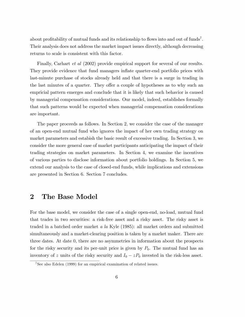
egy of our informed fund manager is now given by:
x� =(v � P0)2�
+
1� z
2+k
2(4)
We now need to make appropriate assumptions about what the market maker
knows about the fund manager�s holding level of the risky security. Since funds are
only required to disclose detailed information about their portfolio holdings at half
yearly intervals13, it seems reasonable to treat holding levels as private information
of the manager. Therefore, we assume that the market maker regards z as a random
variable desribed as: ez � N(z; �2z). We will comment on alternative interpretationsof �2z later in this section.
From the fund manager�s optimal strategy given in equation (4), and remembering
that the expected level of trades by liquidity traders is zero, we have the expected
net trades to be:
�y = Ef 12�[(~v � P0) +
1� �~z + �k] + ~ug
=
1� �z
2+k
2
= k; (by assumption)
which yields the result that k = 1� �z.
We can, then, rewrite the fund manager�s optimal trading strategy as:
x� =1
2�[(v � P0) +
1� �z +
1� ��z]
=(v � P0)2�
+
1� (z � �z)2
+
1� �z (5)
13The six monthly requirement is in U.S. markets. In other markets, mandatory disclosure re-quirements are di¤erent. Also, some funds voluntarily disclose portfolio information at quarterlyintervals.
13
and the market maker�s price schedule as:
P1(y) = P0 + �(y �
1� �z)
= P0 +v � P02
+
1� �(z � �z)
2+ �u (6)
The results above are formalized in the next proposition and show that the basic
insight established in the last section carry over to the case where the market maker
anticpates the trading strategy of the fund manager:
Proposition 2 The expected level of trade in the market for the risky security isproportional to the expected level of the risky security held by the mutual fund at the
commencement of trading. The expected price impact of trade is, however, zero. The
greater the fund�s concern about short-term returns, the higher is the expected level of
trading in the market, ceteris paribus.
The result tells us that as the level of holdings by the mutual fund goes up, more
trade is expected in the market for the risky security. What is important to note is
that this result does not depend in any way on the level of liquidity in the market for
the risk security. Instead, it is the fund�s concern with short-term performance and
the total inventory levels that drive this result. The result suggests that the average
trading volume in equity markets increases with aggregate fund holdings. In addition,
on a proportional basis, this impact is likely to be more visible in the case of security
markets with lower liqudity levels where informed trading is more costly due to price
pressure associated with order �ow.
Note that the fact that the market maker anticipates the manager�s incentives
to boost short-term performance (and sets prices accordingly) does not dampen the
manager�s tendency to trade excessively. In fact, such an anticipation sets up a signal-
jamming situation: if the manager does not follow up with the anticipated level of
non-informational orders, the fund�s NAV may su¤er. Hence, the manager is forced
to trade on the margin not because he hopes to fool the market maker on average
14

but because he does not want to su¤er the price consequences of not submitting
non-information based orders.
Finally, to complete our description of the equilibrium in the market for the risky
security, we need to derive the value of the liquidity parameter in the market maker�s
price schedule. We do this following the procedure outlined in Kyle (1985). Thus,
invoking the properties of the Normal distribution and our assumption on the com-
petition between players in the security markets, we have:
� =Cov(~y; ~v
2�)
V ar(~y)
=12��2v
14�2�2v + �
2 �2z
4+ �2u
where � =
1�
which, on simpli�cation, reduces to:
� =�v
2(�2 �2z
4+ �2u)
12
(7)
With respect to the liquidity parameter, �, note the presence of an extra term,
�2 �2z
4, compared to the expression for the liquidity parameter in Kyle (1985). As
explained above, from the market maker�s point of view, this is the variance of the
non-informational component of the order �ow originating with the mutual fund.
The greater the short term focus on performance, the greater are the incentives for
the mutual fund to try and a¤ect the market clearing price at time 1. However,
variations of trading orders on this account have no information content about future
value and, thus, a competitive market maker regards such variation as noise. Thus,
the uncertainty about the fund�s holdings serves to make a component of its trading
strategy similar to that of liquidity traders and makes, on the whole, the market more
liquid. This implies, in turn, that the component of fund order �ow that depends
on its manager�s informational advantage will be larger in magnitude than in Kyle
(1985). This is because the per unit cost of an order, in terms of its impact on trade
price is now smaller. These observations are presented in the following proposition:
15
Proposition 3 Uncertainty about a fund�s holding of a risky security makes the mar-ket in the security more liquid. This, in turn, implies that informed orders at any
level of private information are larger in scale.
Thsi result leads to an interesting conclusion: it is possible, in our context, to
have both expected and realized trading activity even in the absence of uninformed
liquidity traders. Such trading arises due to two reasons. First, from the market
maker�s perspective, variation in inventory levels is nothing but an endowment shock
for the fund manager. Given our assumption of universal risk-neutrality, however,
an endowment shock by itself should not generate trading since a reallocation of
endowments does not bene�t either the investors or the market maker. However,
this is where the second factor kicks in. Notice that although the trade that takes
place is, ultimately, between the mutual fund investors and the market maker, the
quantity of trade is determined by the mutual fund manager who has an utility
function that is not dependent only on �nal payo¤s. She actually cares about the
temporal distribution of market values of the fund and is willing to distort her trading
strategies in order to maximize her objectives. Her concern with the pattern of prices
over time makes our situation qualitatively similar to an endowment shock in a model
with traders who care about risk. From the no-trade results in Milgrom and Stokey
(1982), we know that such endowment shocks can, indeed, generate trade. It is thus,
the manager�s concern with the short-run performance coupled with the uncertainty
about her portfolio that jointly allow for trade without the participation of separate
uninformed liquidity traders. This leads to the following observation:
Corollary 1 When an fund manager is concerned with short term performance andwhen her inventory of the risky asset is private information, it is possible to have
trade in equilibrium without the presence of liquidity traders.
In the situation we describe, therefore, a market maker receiving an order from
a mutual fund manager is uncertain as to the extent to which this order is driven
by the manager�s informational advantage. She has, thus, no choice but to make a
conjecture in this regard and set prices accordingly. To the extent that he knows
16
the manager�s objective to be short-term performance, he is willing to accomodate
the order with minimal movement in prices. Hence, the more uncertainty in the
manager�s endowment of the risky asset, we should expect to see greater levels of
trade and lesser impact of trade on prices. Of course, in this setting, the mutual fund
manager loses through excessive trading all the gains she expects to make from her
superior information.
In order to see more clearly the bene�ts and costs associated with the fund man-
ager�s trading activity, we need to establish the expected long-term pro�ts of the
investors in the fund. In this also, we follow the methods in Kyle (1985). We take
the point of view of participants in the market and characterize the unconditional
expected pro�ts of the long-term investors. In other words, we are not characterizing
the expected pro�ts of the fund manager who knows what her endowment of ~z is
at time 0 but her unconditional expectation before she acquires her inventory. The
expected long-term pro�ts are given by:
E(�) = E[~z(~v � P0) + ~x�(~v � P1)]
= E[~x�(~v � P1)] since E(~v) = P0
= E[f~v � P02�
+ �(~z + �z)
2gf~v � P0 � �(
~v � P02�
+ �(~z � �z)2
+ ~u)g]
= E[(~v � P0)24�
� �v(z � �z)4
� u(v � P0)2
+�v(~z + �z)
4� ��
2(z2 � �z2)4
� �u�(~z + �z)2
]
=�2v4�� ��
2�2z4
(8)
=�v(�
2 �2z
4+ �2u)
12
2�
�v�2 �
2z
4
2(�2 �2z
4+ �2u)
12
; using � =�v
2(�2 �2z
4+ �2u)
12
=�v(�
2 �2z
4+ �2u)� �v�2
�2z4
2(�2 �2z
4+ �2u)
12
=�v�
2u
2(�2 �2z
4+ �2u)
12
(9)
Note that the expression for expected pro�ts reduces to the one found in Kyle
(1985), �v�u2, when either �2z = 0 or when � = 0. A positive value of �, indicating a
focus on short-term results, serves to decrease the long-term pro�tability of the fund
17
when there is uncertainty about her holdings of the risky security. It is important
to note, though, that in the absence of uncertainty about her inventory position, a
focus on short-term results does not reduce her pro�tability. This is not because
the absence of such uncertainty reduces her deviation from the optimal informational
trade level. Indeed, she still trades based on her inventory position but such trade is
perfectly anticipated by the market maker and, therefore, imposes no price penalty
on her, in equilibrium. In the absence of noise about her inventory, however, liquidity
trading is obviously needed to generate any trade at all.
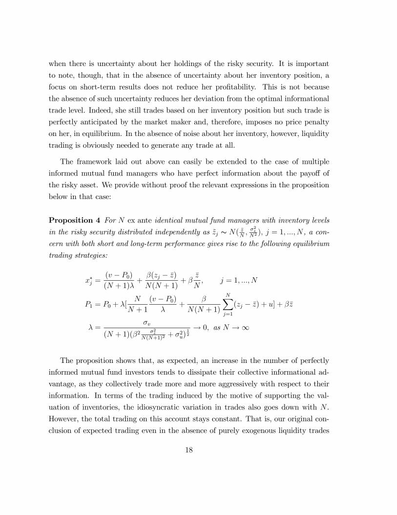
The framework laid out above can easily be extended to the case of multiple
informed mutual fund managers who have perfect information about the payo¤ of
the risky asset. We provide without proof the relevant expressions in the proposition
below in that case:
Proposition 4 For N ex ante identical mutual fund managers with inventory levels
in the risky security distributed independently as ~zj s N( �zN ;�2zN2 ); j = 1; :::; N , a con-
cern with both short and long-term performance gives rise to the following equilibrium
trading strategies:
x�j =(v � P0)(N + 1)�
+�(zj � �z)N(N + 1)
+ ��z
N; j = 1; :::; N
P1 = P0 + �[N
N + 1
(v � P0)�
+�
N(N + 1)
NXj=1
(zj � �z) + u] + ��z
� =�v
(N + 1)(�2 �2zN(N+1)2
+ �2u)12
! 0; as N !1
The proposition shows that, as expected, an increase in the number of perfectly
informed mutual fund investors tends to dissipate their collective informational ad-
vantage, as they collectively trade more and more aggressively with respect to their
information. In terms of the trading induced by the motive of supporting the val-
uation of inventories, the idiosyncratic variation in trades also goes down with N .
However, the total trading on this account stays constant. That is, our original con-
clusion of expected trading even in the absence of purely exogenous liquidity trades
18

still survives and, indeed, becomes relatively more important as N increases. In fact,
as short-term performance evaluation becomes more and more important, the ex-
pected level of trade rises as the market maker takes into account each manager�s
incentive to keep on trading in order to bolster the value of her portfolio. In other
words, trading activity that is meant to enhance the value of an existing portfolio
does not decrease as the market�s become more informationally e¢ cient, although its
price impact does go down14.
We would like to emphasize also the fact that our demonstration that expected
levels of trading are positive when the fund is concerned with its short-term perfor-
mance, has nothing to do with the unobservability of its inventory position. The
unobservability of the inventory of risky assets is only responsible for the deviation in
the fund�s actual trading from a level expected by other market participants. When
the fund�s inventory is common knowledge, there is, of course, no such deviation.
However, its incentive to trade in order to bolster its NAV still remains as strong as
when its inventory is not known. Thus, our results on the magnitude of expected
trade do not depend on our assumption that inventory positions are asymmetrically
known. Our asymmetric information assumption will, however, be more important
in the sections that follow.
4 Inventory as information
In this section, we investigate whether asymmetry of information about the inventory
of the risky assets helps or hurts the mutual fund�s investors or its manager. To
examine this question, we return to the one fund model used earlier, in order to keep
the exposition simple. Given the fund manager knows her own inventory position,
the �rst question to ask is how a commitment to disclose this information before
trading starts a¤ects various parties. Obviously, the competitive market maker�s
payo¤s are una¤ected by such a commitment. Consequently, we examine the e¤ect of
14It is stratightforward to generalize to the case when each fund manager receives a noisy signalof value. In this case, too, the expected trade levels increase with N .
19

a commitment to disclose on the mutual fund�s investors and on its manager�s payo¤s.
Proposition 5 A commitment to disclose the position in the risky asset prior to
submitting trading orders unambiguously helps the long-term pro�ts of investors but
hurts the interests of the fund manager.
Proof: From equation (9), we know that the ex ante expected long-term pro�ts of
the investors is given by: �v�2u
2(�2�2z4+�2u)
12. Clearly, this is monotonically decreasing in the
variance of the inventory information �2z . Thus, a commitment to disclose is in the
interest of the fund�s investors.
The manager, however, is interested in a weighted average of the long-term pro�ts
and the NAV in period 1. The �rst term in her ex ante objective function is given by
E[z(E(P1)� P0)]. Substituting for E(P1) and simplifying this expression yields:
E[z(E(P1)� P0)] = E[z(v � P02
+ ��(z � �z)
2)]
= ��
2E[z(z � �z)] = ���2z
2
Recalling the manager�s objective function as a weighted average of the period 1 NAV
and the long-term expected pro�ts, and using equation (8), we have the value of the
manager�s objective under her optimal trading strategy as:
�
2��2z + (1� )(
�2v4�� ��
2�2z4
)
= (1� )�[ �2v
4�2+ �2
�2z4]
= (1� ) �v
2(�2 �2z
4+ �2u)
12
[2�2�2z4+ �2u]
which is, clearly, increasing in �2z . Therefore, the manager�s ex ante payo¤ in-
creases with the noise in her inventory signal. In other words, she prefers not to
commit to disclose her inventory position. �
20

Even though investor�s may prefer to commit to disclose the fund�s inventory
position, it seems impracticable that it will be possible to monitor such disclosure
very easily. On top of this is the issue of time consistency - the temptation to renege
on such commitments is high. Accordingly, we assume that disclosure of the holdings
of the risky asset will not take place prior to commencement of trading.
In this situation, the fund manager is clearly vulnerable to the designs of other
market participants who may have knowledge of her inventory positions. In other
words, pro�table trading is possible based on either fundamental information on asset
values, or on information regarding the inventory position of the fund. What we have
in mind is the existence of organizations which try to monitor trading by major
funds and tailor their own trading to try and take advantage of the fund�s trading
imperatives. To this end, we modify our base case scenario to allow for a strategic
investor who gets to observe the inventory position of the fund manager before the
commencement of trading. This strategic trader gets to submit a market order based
on his information on inventory. To isolate the value of inventory information by
itself, we assume that the trader has no private payo¤ information about the risky
asset. We can, then, derive the following result:
Proposition 6 Information on the inventory holdings of the mutual fund is valuablefor trading. The ex ante value of such information is proportional to �2z .
Proof: To simplify the notation, we consider the case when the expected inventorylevel is 0 and the initial price level, P0 = 0. The proof is easily extended to the general
case. Consider, then, the situation of a mutual fund manager who has an inventory
level, z, of the risky security. The strategic trader, who has access to this information,
places an order of xs. In equilibrium, this order is correctly anticipated by the mutual
fund manager and, hence, building on the analysis of the earlier section, we can show
that the order strategy of the fund manager will now be given by:
x� =v
2�+ �
z
2� xs2
21
For the strategic trader, his order strategy will be chosen to maximize:
xs[0� �E(x� + xs)]
since, from his perspective, E(v) = 0.
Setting the �rst derivative to zero yields:
��(E(x�) + 2xs) = 0
Substituting for E(x�) from above yields:
�z
2+3xs2= 0
) xs = ��
3
which, on substitution into the trader�s objective function, yields an expected
pro�t level of:
�s =1
9��2�2z
Since the market maker makes zero expected pro�ts, the pro�ts for the strategic
trader must come at the expense of the fund manager and her investors. �
It is clear then, that in a market populated by mutual funds whose managers care
about their short-term performance as measured by their NAVs, there is scope for
pro�table trading even without any knowledge of fundamental values of risky assets.
Hence, it pays an investor to engage in costly search for such information. Similarly, it
pays the fund manager to hide his inventory information from potential competitors,
even though this information is not, by itself, payo¤ relevant.
22
5 Closed-end Funds
Up to this point, we have talked about open-end funds, although we have not explicitly
accounted for withdrawals or deposits by investors at date 1. As alluded to earlier,
our choice not to model fund �ows for the mutual fund is partly dictated by a desire
to directly compare and contrast the performance of open-end and closed-end funds.
Unlike an open-end fund, a closed-end fund does not permit an investor to withdraw
his funds before the liquidation of the fund15. To satisfy investors�liquidity needs,
however, the fund is listed on a stock exchange and its shares are actively traded. As
mentioned in the introduction, closed-end funds typically trade at a discount to the
NAV of the fund, although some funds occasionally trade at a premium. Discounts
of 10 to 20 per cent are quite common and have been regarded as an anomaly in
markets that have otherwise been regarded as reasonably e¢ cient. The persistence of
the discrepancy between market values and NAV of closed-end funds has been called
the � closed-end fund puzzle�. In this section, we demonstrate that our model is
capable of generating the prediction of an expected discount for closed-end funds.
The earliest attempts at explaining the closed-end fund puzzle relied on the hy-
pothesis that the NAV of funds may overestimate the market value of the fund portfo-
lio. Three main classes of factors have been explored in this approach: agency costs,
tax liabilities and the illiquidity of asset holdings. The agency cost theories argue
that NAV �gures do not take into account management expenses and expectations of
future managerial performance, while market values do. In the tax explanations, it
is argued that the tax liabilities on unrealized capital gains are not captured by the
NAV, while the market prices have these impounded in them. The liquidity approach
focuses on the holdings of restricted or letter securities to argue that reported NAVs
may overestimate the actual market values of these illiquid holdings. While each
of these explanations has signi�cant conceptual appeal, extensive empirical analy-
sis has failed to demonstrate convincingly that they explain a signi�cant amount of
the magnitude of these discounts. In addition, time-series properties of the discount
have been found to be related to both overall market performance and to the market
15Alternatively, a closed-end fund may be opened up. In our simple, three date model, we do nothave to distinguish between these two outcomes.
23

performance of small stocks.16
Partially motivated by the failure of these approaches to explain satisfactorily
either the magnitude or the time-series properties of the discount, Lee, Shleifer and
Thaler (1991), advance the case for a behavioral approach. Building on the ideas in
Zweig (1973) and Delong, Shleifer, Summers and Waldmann (1990), they argue that
�uctuations in the sentiment of small investors may be responsible for deviations of the
market value from fundamental value. Such deviations are not subject to exploitation
by arbitraguers because, in the presence of unpredictable sentiments, attempts to
arbitrage deviations become inherently risky. Moreover, Lee, Shleifer and Thaler
(1991) argue that the investor sentiment models are consistent with the patterns in
the time-series variation of these discounts, while earlier approaches fail to satisfy in
this regard.17 In our explanation outlined below, we show that fund discounts and
premia may exist even in a world in which taxes and dissipative transaction costs are
not present and in which correlated investor actions do not serve to move prices of
closed-end funds. Providing empirical support for our arguments is, however, beyond
the scope of the current paper.
We need only minor modi�cations to our basic model to cover the case of closed-
end funds. Since fund manager compensation for closed-end funds is also usually
related to funds under management, we do not need to modify the manager�s objective
function from the earlier sections. Also, since we did not account for deposits or
withdrawals by investors, we do not need to modify our structure to �t the case of
closed-end funds. However, we do need to specify the mechanics of how and when a
closed-end fund is priced in the market. The assumptions we make in this regard are
the simplest possible. Obviously, at time 2, there is no discrepancy between the NAV
of the fund and its market price, since payo¤s are realized at this point. At time 1, we
assume that the prices of both the fund and the risky asset are established in market
16Malkiel (1977) studies the in�uence of several of the factors reported above, while Barclay,Holderness and Ponti¤ (1993) focus on agency costs. Brickley, Manaster and Schallheim (1991) andPonti¤ (1995) study the impact of tax issues, while Ponti¤ (1996) studies the in�uence of tradingcosts.17See, however, Banerjee (1996), Oh and Ross (1994), Chordia and Swaminathan (1997) and
Spiegel (1998) for alternate approaches to explaining closed-end fund disounts and their time-seriespatterns.
24

trading before the fund uses the closing market price of the security to compute
and announce its NAV18. However, we do not explicitly model the price discovery
mechanism of the closed-end fund, since we do not want to introduce e¤ects of any
kind of transactions costs into this process. Consequently, we simply assume that
investors establish the price of the fund based on the net order �ow in the market for
the risky security and its clearing price. The investors being risk neutral, then, the
price of the closed-end fund is, then, simply its expected time 2 value, conditional
on the price in the market for the risky security. At time 0, the NAV of the fund is
already given by I0 and we assume that the price of the fund is its (unconditional)
expectation of the fund�s period 2 payo¤s.
With these simple extensions in place, we are ready to state the central result in
this section:
Proposition 7 At time 1, the closed-end fund�s price exceeds its expected NAV by
the factor �2(2�2u� ��2z). Therefore, for ��2z > 2�2u, the closed-end fund is expected to
have a discount from its Net Asset Value, while a premium is expected if the inequality
goes the other way.
Proof:
At time 1, after the order �ow, y, and the market price, P1, for the risky security
are observed, but before the NAV has been announced, the price of the fund is given
by:
I0 + Ey[z(v � P0) + x(v � P1)]
= I0 + Ey[z(v � P1) + x(v � P1) + z(P1 � P0)]
= I0 + Ey[(x+ z)(v � P1)] + E[z(P1 � P0)]
where the operator Ey(�) denotes the expectation conditional on y. But I0+Ey[z(P1�P0)] is nothing but the expected NAV of the fund. Hence, the di¤erence between the18Observe that we continue to use the single fund and single risky security structure of our basic
model in this section.
25

market price of the fund and its expected NAV is given by Ey[(x+ z)(v�P1)]. Now,recalling that Ey(v) = P1, we can rewrite this expression as:
E[(x� �xy)(v � �vy)] + E[(z � �zy)(v � �vy)] (10)
where �xy, �zy, and �vy denote the conditional expectations of these variables. Recall
that, by the properties of the Normal distribution, we can denote the generic condi-
tional expectation of a variate as:
�my = �m+�my�2y(y � �y)
Thus, we can write the �rst term in equation (10) as:
E[(x� �xy)(v � �vy)] = E[(x� �x��xy�2y(y � �y))(v � �v � �vy
�2y(y � �y))]
= E[(x� �x)(v � �v)� �xy�vy�2y
]
=�2v2�(1� �
2x
�2y) =
�2v�2u
2��2y
since y = x + u. However, we know from the de�nition of � that �2v4�2
= �2 �2z
4+ �2u,
while we must have �2y = �2x + �2u =
�2v4�2+ �2 �
2z
4+ �2u. Using these equalities in the
equation above gives us the value of E[(x� �xy)(v � �vy)] = ��2u.
Similarly, the second term in equation (10) can be shown to be:
E[(z � �zy)(v � �vy)] = E[(z � �z ��zy�2y(y � �y))(v � �v � �vy
�2y(y � �y))]
= 0� ��2z�
2v
4��2y= ��
2��2z
26
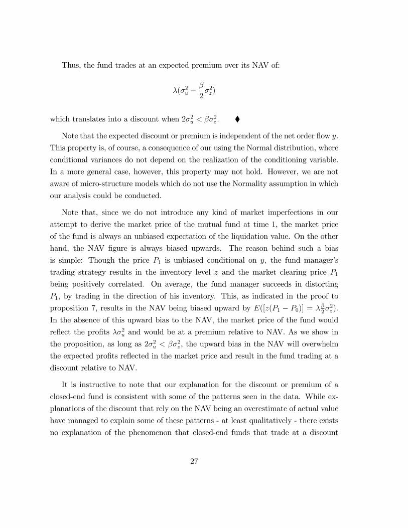
Thus, the fund trades at an expected premium over its NAV of:
�(�2u ��
2�2z)
which translates into a discount when 2�2u < ��2z . �
Note that the expected discount or premium is independent of the net order �ow y.
This property is, of course, a consequence of our using the Normal distribution, where
conditional variances do not depend on the realization of the conditioning variable.
In a more general case, however, this property may not hold. However, we are not
aware of micro-structure models which do not use the Normality assumption in which
our analysis could be conducted.
Note that, since we do not introduce any kind of market imperfections in our
attempt to derive the market price of the mutual fund at time 1, the market price
of the fund is always an unbiased expectation of the liquidation value. On the other
hand, the NAV �gure is always biased upwards. The reason behind such a bias
is simple: Though the price P1 is unbiased conditional on y, the fund manager�s
trading strategy results in the inventory level z and the market clearing price P1being positively correlated. On average, the fund manager succeeds in distorting
P1, by trading in the direction of his inventory. This, as indicated in the proof to
proposition 7, results in the NAV being biased upward by E([z(P1 � P0)] = ��2�2z).
In the absence of this upward bias to the NAV, the market price of the fund would
re�ect the pro�ts ��2u and would be at a premium relative to NAV. As we show in
the proposition, as long as 2�2u < ��2z , the upward bias in the NAV will overwhelm
the expected pro�ts re�ected in the market price and result in the fund trading at a
discount relative to NAV.
It is instructive to note that our explanation for the discount or premium of a
closed-end fund is consistent with some of the patterns seen in the data. While ex-
planations of the discount that rely on the NAV being an overestimate of actual value
have managed to explain some of these patterns - at least qualitatively - there exists
no explanation of the phenomenon that closed-end funds that trade at a discount
27

start out at a premium to NAV after their initial public o¤ering19. This portion of
the puzzle is particularly troublesome from the point of view of e¢ cient markets since
no rational investor should buy into a newly formed closed-end fund while clearly an-
ticipating the fall in prices later. However, our analysis points out that it is not the
price of the fund that is biased but that it is the NAV that is biased upwards. At
the time of the initial public o¤ering, when information asymmetry about the fund�s
holdings is very little, the uncertainty in its holdings of the risky asset is clearly low.
Assuming the fund manager is viewed as having some informational advantage, we
should expect the fund to trade at a premium to NAV at this point in time. As
the fund gets to implement its portfolio strategy, the uncertainty with respect to its
holdings of the risky asset grows. In such a situation, provided the condition derived
above is satis�ed, the fund may very well trade at a discount to its NAV. Thus, we
have the following corollary:
Corollary 2 A closed-end fund managed by a manager who is presumed to be in-
formationally advantaged, will start out at a premium to NAV which will decrease
over time as its inventory position in the risky asset becomes more uncertain. At
su¢ ciently high levels of the uncertainty in its inventory position, the fund will be
expected to trade at a discount to its NAV.
In our world, therefore, there is nothing surprising about either a closed-end fund
trading at a discount to its NAV, nor in its transition from a state in which it trades
at a premium to one in which it trades at a discount. The obvious question to ask,
then, is about what would happen if a closed-end fund were to announce a transition
to an open-end status. Clearly, then, investors would have the right to cash out at the
NAV of the fund. Under the assumption that such a transition is feasible, meaning
that such an open-end fund would not immediately trigger an unsustainable rush of
redemptions, the value of the fund would rise towards its NAV. However, its NAV
would not fall since neither its inventory position, nor the market prices of its holdings
would be a¤ected by the announcement. Thus, we have:
19See, for example, Peavy (1990) for a description of this phenomenon.
28

Corollary 3 When a conversion from a closed-end structure to an open-end one is
made for a fund trading at a discount, its market value is expected to rise towards its
NAV. However, the NAV should not react to such an announcement.
As Lee, Shleifer and Thaler (1991) point out, it is not only the fact that closed-
end funds usually sell at a discount to their NAVs that is a puzzle. The puzzle
is augmented by several other side observations. Important among these are the
transition from a premium to discount status after funds�initial public o¤erings and
the movement in fund value towards NAV on the announcement of the fund�s opening
up. At least in the context of our simple model, both of these puzzles are easily
explained.
6 Implications and Extensions
The analysis up to this point has used the market micro-structure model of Kyle
(1985) and con�ned itself, for the most part, to the case of single mutual fund and
a single risky security. Clearly, these results need to be extended to more general
cases for our conclusions to pass muster. However, we are currently in the process of
undertaking these extensions. Below, we provide previews of several extensions that
we intend to incorporate in future versions of this paper.
Extension to other market structures: Although we have used the structure of Kyle
(1985) in the analysis, many of our results should hold without the structure of a
market maker who sees the net order �ow. For example, suppose that the market
maker setting prices for the risky security imposes a price schedule for inventory pur-
poses. Even in this case, the analysis of the mutual fund manager�s trading strategy
remains essentially similar to the case we have analyzed and the clearing price reveals
information to market participants about the value of the fund itself. Although the
liquidity parameter, �, in this case is determined by means other than the one we
have analyzed, there is no reason why most of our analysis would not survive in this
alternate case.
29

Extension to multiple securities: At a basic level, the extension to the case of multiple
securities should be straightforward, as long as the position in each security can be
independently analyzed via an assumption of independent price setting in markets for
each security in the fund�s portfolio. However, we have not yet attempted a formal
analysis of the multiple-security case. Note, however, that in the multiple security
case, we would expect discounts or premia for closed-end funds to be even more
tightly distributed around expected values. This should arise due to the reduction in
idiosyncratic variances associated with individual securities.
Extension to multiple funds: The text contains a preliminary analysis of extending
our results to the multi-fund case. However, this analysis is somewhat incomplete
in that we assume a symmetric, independent structure for mutual fund holdings. In
reality, there is likely to be an upper bound on the variance of the holdings of the
mutual fund sector as a whole. Consequently, the determination of � in this setting
may require some modi�cations.
Analyzing the choice between mutual fund structures: Clearly, our analysis has impli-
cations for the choice of structure chosen by a mutual fund manager who is about the
raise funds to manage on behalf of investors. Consider, for example, whether she will
choose to go with exit fees or not in case she chooses an open-end structure. Clearly,
if she can commit to reduce her incentives for short term results and can convince
investors of her superior abilities, the market value of her fund may be higher than
her expected NAV. In such a case, to reduce opportunism on the part of investors
who might want to enter the fund at the expense of existing investors, she may de-
cide to charge an entry fee. On the other hand, if the market value of her fund is
expected to be less than the NAV, similar reasoning demands that she consider the
introduction of exit fees. A similar issue arises with respect to her choice between an
open-end and a closed-end structure. Clearly, without exit fees, it is not feasible to
run an open-end fund when one expects the trading decisions of managers to lead to
discounts since opportunist investors may choose to redeem early. Thus, we would
expect more closed-end funds to be exactly those in which the managers/originators
concluded ex ante that the fund would likely be trading at a discount. On the other
hand, without fees of some kind, no open-end fund would be sustainable unless the
30

managers anticipated the fund being valued by the market at a premium to NAV.
This argument, in itself, lends support to the likelihood of �nding closed-end funds
being at a discount relative to their NAVs.
Our results clearly have the greatest impact in markets that are less liquid. It
is not surprising, therefore, to note that closed-end funds are more prevalent in less-
developed capital markets and that closed-end funds in the United States tend to
have more small company shares in their portfolios than open-end funds. However,
it is important to note that our analysis of the manager�s trading strategy does not
require us to restrict our attention to the case of relatively illiquid securities. The
extensions outlined above will enable us to answer the obvious questions as to how
important our conclusions may be in the context of markets with di¤erent degrees of
liquidity.
7 Conclusion
We have analyzed the trading decisions of a mutual fund manager in a simple model
using a variation of well known market-microstructure model. As a result, we have
been able to integrate the analysis of mutual fund trading decisions with issues of mar-
ket liquidity that are well studied in the micro-structure area. Our main analytical
contribution has been to introduce a modeling strategy that manages to parameter-
ize the short-horizon focus of fund managers in a simple way. In doing so, we have
demonstrated that trading activity is expected to increase along with holdings by
mutual funds in the economy and along with increases in short-term performance
measurement of mutual fund managers. Our model shows that the di¤erential incen-
tives between mutual fund managers and long-term investors alone is able to generate
trading in a world where diversi�cation to reduce risk is not a motive for trade. In
doing so, our analysis highlights the role that large mutual funds with substantial
holdings may play in the price-setting process in �nancial markets.
We have also shown that the closed-end fund puzzle may be explained with the
help of our model and that inventory risk, coupled with trading in �nancial markets by
31

players who are interested in the marked-to-market value of their assets may account
for premia and discounts for closed-end funds. These conclusions are reached even
in the absence of factors that have already been stressed in the existing literature
that has tried to explain the deviation in prices of funds from their Net Asset Values.
We view inventory risk as another factor that contributes to the explanation of the
closed-end fund puzzle and not an alternative to extant explanations.
32
References
Banerjee, S., 1996, Discounts and premiums in closed-end funds, Working Paper,
Brunel University.
Barclay, M., C. Holderness and J. Ponti¤, 1993, Private bene�ts from block ownership
and discounts on closed-end funds, Journal of Financial Economics 33, 263-291.
Berk, J. and R. Green, 2004, Mutual fund �ows and performance in rational markets,
Journal of Political Economy, 112, 1269-1295.
Brickley, J., S. Manaster and J. Schallheim, 1991, The tax-timing option and dis-
counts on closed-end investment companies, Journal of Business 64, 287-312.
Carhart, M., R. Kaniel, D. Musto, and A. Reed (2002), Leaning for the Tape: Evi-
dence of Gaming Behavior in Equity Mutual Funds, Journal of Finance, 57, 2, 661-
693.
Chordia, T. and B. Swaminathan, 1996, Market segmentation, imperfect information
and closed-end fund discounts, Working Paper, Owen Graduate School of Manage-
ment, Vanderbilt University.
Chevalier, J. and G. Ellison, 1997, Risk taking by mutual funds as a response to
incentives, Journal of Political Economy, 105, 1167-1200.
Easley, D. and M. Ohara, 1987, Price, trade size and information in securities mar-
kets, Journal of Financial Economics,
Delong, J. B., A. Shleifer, L.H. Summers, and R. J. Waldmann, 1990, Noise trader
risk in �nancial markets, Journal of Political Economy 98, 703-738.
Diamond, D. and P. Dybvig, 1986, Banking theory, deposit insurance and bank reg-
ulation, Journal of Business
Dimson, E. and C. Minio-Kozerski, 1999, Closed-End Funds: a survey, Financial
Markets, Institutiions and Instruments, 9, 1-41.
Dow, J. and G. Gorton, 1997, Noise Trading, delegated portfolio management, and
economic welfare, Journal of Political Economy, 105, 1024-1050.
Edelen, R. M, 1999, Investor �ows and the assessed performance of open-end mutual
funds, Journal of Financial Economics, 53, 439-466.
33
Ho, T. and H. Stoll, 1981, Optimal dealer pricing under transactions and return
uncertainty, Journal of Financial Economics, 9, 47-73.
Huddart, S. J., 1998, Reputation and performance fee e¤ects on portfolio choice by
investment advisors, Journal of Financial Markets 2, pp..
Kyle, A., 1985, Continuous auctions and insider trading, Econometrica 53, 1315-1336.
Lee, C. M. C., A. Shleifer and R. H. Thaler, 1991, Investor sentiment and the closed-
end fund puzzle, Journal of Finance 46, 75-109.
Malkiel, B. G., 1977, The valuation of closed-end investment company shares, Journal
of Finance 32, 847-859.
Nanda, V., M. P. Narayanan and V. Warther, 1998, Liquidity, investment ability, and
mutual fund structure, Working Paper, University of Michigan Business School.
Nanda, V. and R. Singh, 1999, Mutual fund structures and the pricing of liquidity,
Working Paper, University of Michigan Business School.
Oh, G. and S. Ross, 1994, Asymmetric information and the closed-end fund puzzle,
Working Paper, University of Iowa.
Peavy, J. W., 1990, Returns on initial public o¤erings of closed-end funds, Review of
Financial Studies 3, 695-708.
Ponti¤, J., 1995, Closed-end fund premia and returns implications for �nancial market
equilibrium, Journal of Financial Economics 37, 341-370.
Ponti¤, J., 1996, Costly arbitrage: evidence from closed-end funds, Quarterly Journal
of Economics 111, 1135-1151.
Sirri, E. and P. Tufano, 1998, Costly Search and Mutual Fund Flows Journal of
Finance, 53, 1589-1622.
Spiegel, M., 1998, Closed-end fund discounts in a rational agent economy, Working
Paper, Haas School of Business, University of California at Berkeley.
von Thadden, E, 1995, Long-term contracts, short-term investment and monitoring,
Review of Economic Studies, 62, 557-575.
34

Zweig, M. E., 1973, An investor expectations stock price predictive model using
closed-end fund premiums, Journal of Finance 28, 67-87.
35
Recommended