1
Market Competition and Price Clustering: Evidence from the ETF Markets
Wei-Peng Chen, Huimin Chung, Her-Jiun Sheu and Shufang Shiu*
_____________________________________________________________________
ABSTRACT
Price clustering is a widely-recognized phenomenon within financial markets, with some
studies in this area suggesting that for specific reasons, prices may cluster at certain
numbers. This paper explores the outcome on price clustering stemming from the
commencement of trading in ‘exchange traded funds’ (ETFs) on the New York Stock
Exchange (NYSE). The results of this study show that trading characteristic variables,
such as the effective percentage spread, the percentage of medium-sized trades and the
asymmetric information component, could well explain the changes in price clustering.
There was a discernible reduction in price clustering amongst ETFs traded on the
American Stock Exchange (AMEX), which may be attributable to improvements in
market liquidity leading to a reduction in the asymmetric information component brought
about by increased market competition. Making pricing information available to the public
and thereby alleviating informed trading may be a feasible explanation for the changes that
occurred in the NYSE following the commencement of ETF trading. More specifically,
our results support the claims of the price resolution hypothesis (Ball et al., 1985) and the
negotiation hypothesis (Harris, 1991).
Keywords: Price clustering; Market competition; ETFs; Microstructure.
* Wei-Peng Chen (the corresponding author) is at the Department of Management Science, National Chiao Tung University, 1001 Ta-Hsueh Road, Hsinchu 30050, Taiwan, Tel: +886-3-5712121 ext.57070; Fax: +886-3- 5733260; e-mail: [email protected]; Huimin Chung is at the Graduate Institute of Finance, National Chiao Tung University, Her-Jiun Sheu and Shufang Shiu are at the Department of Management Science, National Chiao Tung University.

2
1. INTRODUCTION
Financial asset prices will often tend to cluster at certain numbers, a phenomenon
which occurs as a result of traders using a discrete set of prices to specify the terms of
their trades. Under a constrained minimum tick size, and in the absence of both market
friction and bias, prices should be uniformly distributed across every likely value;
nevertheless, observed prices are invariably rounded off, either up or down. The
resultant clustering of trade prices, which is the tendency for certain prices to be
observed with greater frequency than others, is commonplace; indeed this is already
well documented in the literature both within and across markets (Kandel et al., 2001;
Ikenberry and Weston, 2005; Ohta, 2006).
One of the main areas of focus within the studies on price clustering over the past
two decades has been in-depth investigation of the nature of clustering. According to
these studies, clustering can be the result of many factors, such as human bias
(Hornick et al., 1994), the attraction of specific numbers (Goodhart and Curcio, 1991),
or even cultural factors influencing the preference for certain numbers (Brown et al.,
2002); there is also the likelihood of collusion between market makers (Christie and
Schultz, 1994) or differences between market structures (Grossman et al., 1997).
Nevertheless, the most common explanations used in the prior research to
illustrate the occurrence of price clustering have been the price resolution hypothesis
(Ball et al., 1985) and the negotiation hypothesis (Harris, 1991). Ball et al. (1985)
argued that the degree of price resolution was a function of the amount of information
3
in the market, as well as the level and variability of the price; the resultant uncertainty
with regard to the underlying value of securities would make accurate pricing less
valuable and would thereby induce traders to submit orders at round-number prices.
Harris (1991) advocated the negotiation hypothesis arguing that, based upon the
price resolution hypothesis, the size of the discrete price set was determined by an
investor’s trade-off between the negotiation costs and the loss of the benefits from the
trade. Thus, if traders used a coarse set of prices, negotiation costs would be lower and
benefits may be lost. According to the negotiation hypothesis, such lost benefits from
the trade are likely if little dispersion exists amongst trade reservation prices, such as
when the value of the underlying assets are well known; conversely, traders using a
coarser discrete price set may not suffer from such losses when the existence of
asymmetric information between traders is obvious. This implies that price clustering
may be more significant in the less liquid markets because of the greater amount of
asymmetric information existing in trade reservation prices.
According to the negotiation hypothesis, market quality is an important factor
affecting price clustering (Harris, 1991; Grossman et al., 1997; Martinez and Tse,
2006). In their study of multi-market effects on market liquidity, Chowdhry and Nanda
(1991) presumed that market makers compete to offer the lowest cost of trading in
their location, with the competition for multiple exchange trading inducing market
makers to take action to ensure that price information is made public, thereby also
reducing insider trading.

4
Furthermore, by making information available in such a way, in addition to
discouraging informed trading, it may also attract liquidity traders, thereby improving
market liquidity. An important recent development in this area was the commencement
of trading in unlisted securities under the ‘unlisted trading privileges’ (UTPs) in the
New York Stock Exchange (NYSE).1 On 31 July 2001, the NYSE began trading the
three most active ‘exchange traded funds’ (ETFs), the NASDAQ-100 Trust Series I
(QQQ), the Standard and Poor’s Depository Receipt Trust Series I (SPYs) and the
Dow Jones Industrial Average Trust Series I (DIAs), listed on the American Stock
Exchange (AMEX) on a UTP basis. Under the UTP framework, a stock listed on the
AMEX can also trade on other exchanges without dual listing. The commencement of
trading in these three unlisted securities in the NYSE provides a unique opportunity
for us to study the impact of market competition on price clustering and to test the
theoretical hypotheses.
This study sets out to investigate the relationship between price clustering and
market competition in the ETF markets. We aim to address two major research issues:
(i) determination of the effects of market competition on the level of price clustering;
and (ii) the reason why such market competition leads to changes in price clustering.
Whilst most of the prior studies on the effects of implementation of the UTP system
have tended to focus on the issue of its impacts on market quality (Khan and Baker,
1993; Boehmer and Boehmer, 2003; Tse and Erenburg, 2003), to the best of our
1 An ‘unlisted trading privilege’ (UTP) is a right provided by the Securities Exchange Act of 1934 which permits securities listed on any national securities exchange to be traded by other such exchanges.
5
knowledge, very few studies have set out to examine the changes which occur in price
clustering within multi-market competition.2
Extending the prior studies on the influence on market quality stemming from
UTP implementation, this study sets out to provide detailed analysis of the price
clustering of ETF trades on the AMEX and NYSE. We expect that such trading will be
particularly informative, partly because the NYSE is very similar to the AMEX in
structure, organization, trading protocols, and so on; in other words, both exchanges
are traded simultaneously, whilst the prices at which they are traded are almost
perfectly correlated. Therefore, many factors which impact upon the market
mechanism can be excluded from our analysis. Given the comprehensive analysis in
price clustering undertaken in this study, the results may contribute to the growing
understanding of how, and to what extent, the interactions in price clustering were
affected by the introduction of UTP, through the resultant improvements in market
liquidity, so as to provide a better understanding of price clustering in multi-market
trading conditions.
In this paper, we analyze the changes in price clustering in the pre- and post-UTP
periods using a regression model. Considering the likelihood of the simultaneous
relationship between spreads and clustering, we employ the generalized method of
moments (GMM) approach, with instrumental variables, to obtain more efficient
2 The prior empirical literature has tended to focus mainly on issues relating to changes in market quality resulting from the simultaneous trading of derivatives in both the electronic trading system and the open-outcry system (Tse and Zabotina, 2001; ap Gwilym and Ailbo, 2003; Chung and Chiang, 2006; Martinez and Tse, 2006).

6
estimates and more robust test results, since this places no restrictions on either the
conditional or unconditional variance matrix of the disturbance term. Under the GMM
framework, we can obtain the asymptotically efficient estimator without making any
additional assumptions, which enables us to obtain results that are particularly robust.
Utilizing this research methodology, the results of our study show that there was a
reduction in the extent of price clustering after the NYSE entry, and that both the
asymmetric information component and the percentage of medium-sized trades are
significant explanatory factors in price clustering. This may stem from a reduction in
the asymmetric information component and improvements in market liquidity through
the resultant market competition, which is consistent with the negotiation hypothesis.
The remainder of this paper is organized as follows. A review of the related
literature is undertaken in the next section, followed by a description of the data and
the research methodology adopted for our study. The penultimate section presents the
empirical results of our research, with the final section providing some concluding
remarks drawn from this study.
2. RELATED LITERATURE
2.1 Price Clustering
A tick size for each commodity (such as futures, options and shares traded) is set by
the relevant exchange; nevertheless, the official tick size can sometimes be subverted
by market investors who choose to use a larger tick size, which leads to ‘price
clustering’. The phenomenon of price clustering is very common in various financial
7
markets; hence, it has already been well documented within the literature on financial
markets, such as the US stock markets (Ikenberry and Weston, 2005), the Tokyo Stock
Exchange (Ohta, 2006), underwritten offerings (Yeoman, 2001), initial public offerings
(Kandel et al., 2001), foreign exchange markets (Goodhart and Curcio, 1991; Osler,
2003), the London gold market (Grossman et al., 1997), futures markets (ap Gwilym
and Alibo, 2003; Schwartz et al., 2004; Chung and Chiang, 2006), and so on. The
variables/results of the relevant studies on price clustering are listed in Table 1.
< Table 1 is inserted about here >
ap Gwilym (1998a), Schwartz et al. (2004) and Chung and Chiang (2006) used
time series data to detect the phenomenon of clustering, and the factors potentially
involved, whilst Ohta (2006) used panel data to study price clustering on the Tokyo
Stock Exchange. Other studies, including, Harris (1991), Christie and Schultz (1994),
Aitken et al. (1996), Cooney et al. (2003) and Ikenberry and Weston (2005) all used
cross-sectional data to examine the occurrence of clustering. All of these studies have
made important contributions to the theoretical analysis of price clustering.
However, amongst such profuse research into price clustering, some of the most
compelling studies have focused on the factors accounting for price clustering in
financial markets. In Tversky and Kahneman (1974), it was argued that in some cases,
as opposed to the operation of optimal judgment, certain individuals relied upon a
number of ‘heuristic principles’ to assign probabilities, or to predict values. Kahneman
(1982) went on to further expound the complexity of heuristics within the overall
8
judgment and decision process. Thus, these two studies justified the clustering or
‘over-representation’ of round numbers in asset pricing.
Individuals may, however, prefer certain numbers to others, a phenomenon which
Hornick et al. (1994) referred to as ‘human bias’. In their surveys of self-reported
time-based activities, they found that investors displayed a bias for rounding numbers
to 0 or 5; and indeed, Kandel et al. (2001) subsequently found that investors preferred
round numbers in Israeli IPO auctions. Goodhart and Curcio (1991) and Aitken et al.
(1996) had earlier argued that some numbers had a basic attraction to investors, with
the final digit 0 having a greater attraction than 5, which in turn is more popular than
others; they referred to this as the ‘attraction hypothesis’. Consistent with this
hypothesis, in their examination of price clustering on the London Stock Exchange,
Grossman et al. (1997) found that quotes ending in 0 and 5 were the most frequently
seen. Brown et al. (2002) also noted that even cultural factors could influence the
preference for certain numbers. All of these findings are consistent with the thinking of
Ikenberry and Weston (2005) on certain prominent numbers playing an important role
in explaining the tendency for stock price clustering within the NYSE.
It is also possible, however, that some traders use round numbers with specific
intention. The ‘price resolution hypothesis’ proposed by Ball et al. (1985) argues that
price clustering may come about as a result of the achievement of the optimal degree of
price resolution. Higher price volatility leads to greater clustering, because investors
wish to deal quickly with all trades, which will normally lead to less precise valuations.

9
Loomes (1988) went on to find that most subjects dealt with their ‘sphere of
haziness’ by rounding their valuations in order to simplify the overall trading process;
this proposed ‘haziness and bounded rationality hypothesis’ also has explanatory power
in price clustering. The same observation applies to Ohta (2006), who examined the
clustering phenomenon on the Tokyo Stock Exchange under different trading
mechanisms, and concluded that the intraday patterns of price clustering during
continuous auction and call auction were all consistent with the ‘price resolution
hypothesis’.
Harris (1991) observed that uncertainty in the US stock markets caused market
makers to round off their quotations, which could in turn lead to greater price
clustering; therefore, clustering may increase under more volatile and less liquid
market conditions, thereby reducing negotiation costs; Hameed and Terry (1998) also
reported evidence in support of this ‘negotiation hypothesis’. Grossman et al. (1997)
offered an extension of the ‘price resolution/negotiation hypothesis’ to the cost of
maintaining trade liquidity, suggesting that when quotes and trades were infrequent,
the value of the security may be more indeterminate. Therefore, in order to simplify
the negotiation process, market makers would prefer to round off their quotation
numbers, which would consequently induce more clustering.
It had earlier been regarded as quite astonishing when Christie and Schultz (1994)
found evidence of extreme clustering within certain NASDAQ stocks, since this
suggested that NASDAQ dealers were implicitly colluding to maintain wider bid-ask
10
spreads than those that would prevail under full competition. Following on from these
earlier empirical findings, Christie et al. (1994), Barclay (1997), Bessembinder (1997)
and Cooney et al. (2003) all reported consistent results. Conversely, however, in their
examination of several competitive markets, Grossman et al. (1997) found that the
differences in the extent of clustering simply reflected the differences in market
structures, and provided no evidence to support the existence of collusion between
market makers on the NASDAQ; they concluded that there was nothing unusual in
either the extent of the clustering or the cross-sectional variation in clustering on the
NASDAQ.
Progressive trading mechanisms are also leading to improvements in the clustering
phenomenon. For example, ap Gwilym et al. (1998b) examined price clustering in four
long-term government bond futures on the London International Financial Futures
Exchange (LIFFE); this was subsequently followed by a further survey on FTSE 100
Stock Index futures on the LIFFE (ap Gwilym and Alibo, 2003), in which they
attempted to determine whether there were differences in price clustering behavior
following the transfer of futures contract from floor trading to the electronic trading
system. They found that price clustering fell sharply after the introduction of automated
trading, with such changes resulting from a reduction in the effective tick size.
Chung and Chiang (2006) subsequently provided evidence of reduced clustering in
their investigation of the DJIA, S&P 500 and NASDAQ-100 indices. They noted that
those trading mechanisms which involved higher levels of human participation, such as

11
open-outcry markets, could well lead to increased incidences of price clustering.
However, an alternative viewpoint put forward by Martinez and Tse (2006) was that
price clustering was slightly more concentrated in electronic gold futures contracts; thus
suggesting that market liquidity was a major factor determining price clustering.
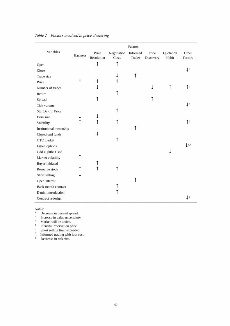
Based upon our review of the prior literature (above), the factors justifying the
possible changes in any of the numerous variables affecting price clustering are
summarized in Table 2.3
< Table 2 is inserted about here >
2.2 Market Competition under Different Trading Mechanisms
The promulgation of the Securities Act Amendments of 1975, which facilitated the
establishment of the National Market System (NMS) in the same year, encouraged the
fair and efficient handling of securities transactions. Several studies were subsequently
undertaken focusing on market quality and efficiency under different market
mechanisms. Chowdhry and Nanda (1991), for example, investigated some of the issues
relating to the trading of a single security within multiple markets; as noted earlier, they
presumed that the competition for multiple-market trading induced market makers to
take action, such as ensuring that price information was made public and thereby
reducing insider trading, and as a result, offering the lowest costs of trading at their
location and maximizing the revenue earned over time as a function of trading volume.
3 It is clear that in addition to the factors of haziness, price-resolution, negotiation costs and psychology, which largely interpret the possible clustering variations, there are still some other factors that could justify the variations; we show these factors in the last column of Table 2 and give some brief explanations in the notes.

12
Khan and Baker (1993) also examined the effect of dual trading (through UTPs)
on liquidity and stock returns after the US Congress and the Securities and Exchange
Commission (SEC) had initiated the NMS. They concluded that there were
significantly positive abnormal returns around the SEC’s announcement of a filing for
UTP by the regional exchange, and also inferred that increased competition improved
trading liquidity.
On 20 January 1997, the SEC also began implementation of the new ‘order
handling rules’ (OHR), changing significantly the way in which the NASDAQ handled
orders. Weston (2000) went on to investigate the impact of such market reform,
documenting that it reduced the rents of NASDAQ dealers, diminished the difference
in spreads between the NYSE and the NASDAQ, and resulted in the exit of many
market makers. The results provided strong evidence to show that the OHR reform had
improved competition on the NASDAQ.
Thereafter, on 31 July 2001, the NYSE began trading ETFs under UTPs, with
various studies subsequently providing evidence on the impact of the UTP system on
market quality. Boehmer and Boehmer (2003), for example, suggested that the NYSE
entry led to dramatic improvements in market liquidity and helped to eliminate market
maker rents, but that this did not adversely affect price discovery. Tse and Erenburg
(2003) examined the influence of spread, market quality and price discovery after the
NYSE begin trading QQQs, whilst also investigating whether the NYSE or the AMEX
was dominant, in terms of price discovery, and which of the markets was favored by

13
informed traders after the entry of the NYSE. They concluded that QQQ trading on the
NYSE led to improvements in market quality and price discovery; however, neither
raised trading costs nor fragmented the market. Both of these studies demonstrated
strong approval for the SEC’s execution of the UTP system.
3. DATA AND RESEARCH METHODOLOGY
3.1 Data
Our analysis focuses mainly on the price clustering of ETFs and the relationship, in
terms of market competition, between the AMEX and the NYSE under the UTP
system. The sample ETFs include DIAs, SPYs and QQQs, with the sample period
being split into two sub-periods. For our analysis of price clustering, the sample period
runs from 29 January 2001 to 30 January 2002, thereby straddling the UTP
implementation date by about a six-month period, before and after, and facilitating an
investigation into whether there have been changes in price clustering following the
implementation of the UTP system.4
The ETF data were obtained from the NYSE Trade and Quote (TAQ) database;
this database includes the tick-by-tick quote and trade prices, trading volume and quote
size behind the ‘best bid and offer’ (BBO) prices.5 We use both the regular AMEX and
NYSE quote and trade prices for the ETFs.
4 From 29 January 2001, all stocks traded on the NYSE and the AMEX were subsequently quoted in decimals (i.e., penny pricing or decimalization); therefore, we use the second digit under the decimal point of ETF prices to analyze the degree of price clustering after this date. 5 Ideally, the quote size beyond the BBO needs to be tested before any definitive conclusion can be drawn with regard to market depth; such information is, however, generally unavailable from public databases.
14
In order to ensure the accuracy of our sample data, we delete all trades and quotes
that are out of time sequence. We also omit quotes that meet the following three
conditions: (i) either the bid or the ask price is equal to, or less than, zero; (ii) either
the bid or the ask depth is equal to, or less than, zero; and (iii) either the price or
volume is equal to, or less than, zero. Following Huang and Stoll (1996), we further
minimize data errors by also eliminating trades and quotes meeting the following
criteria: (i) all quotes with negative bid-ask spreads, or bid-ask spreads of size greater
than US$4; (ii) all trades and quotes which took place either before the market opened
or after the market closed; and (iii) all trade, bid and ask prices with consecutive
absolute changes (i.e., absolute returns) of more than 10 per cent.
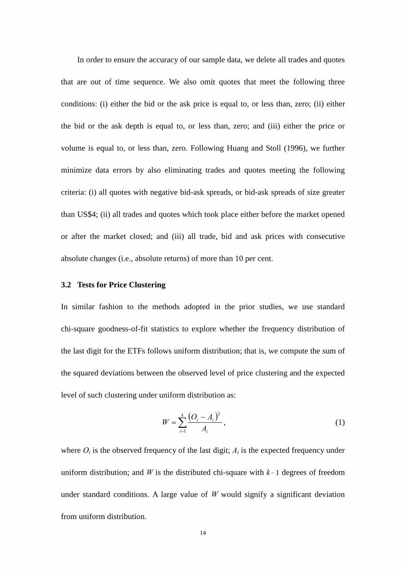
3.2 Tests for Price Clustering
In similar fashion to the methods adopted in the prior studies, we use standard
chi-square goodness-of-fit statistics to explore whether the frequency distribution of
the last digit for the ETFs follows uniform distribution; that is, we compute the sum of
the squared deviations between the observed level of price clustering and the expected
level of such clustering under uniform distribution as:
( )∑=
−=
k
i i
ii
AAO
W1
2
, (1)
where Oi is the observed frequency of the last digit; Ai is the expected frequency under
uniform distribution; and W is the distributed chi-square with k – 1 degrees of freedom
under standard conditions. A large value of W would signify a significant deviation
from uniform distribution.
15
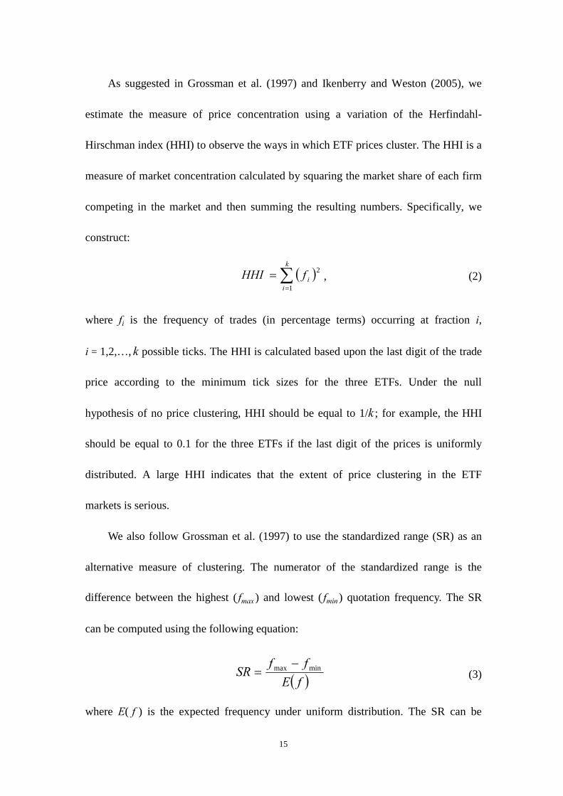
As suggested in Grossman et al. (1997) and Ikenberry and Weston (2005), we
estimate the measure of price concentration using a variation of the Herfindahl-
Hirschman index (HHI) to observe the ways in which ETF prices cluster. The HHI is a
measure of market concentration calculated by squaring the market share of each firm
competing in the market and then summing the resulting numbers. Specifically, we
construct:
( )∑=
=k
iifHHI
1
2 , (2)
where fi is the frequency of trades (in percentage terms) occurring at fraction i,
i = 1,2,…, k possible ticks. The HHI is calculated based upon the last digit of the trade
price according to the minimum tick sizes for the three ETFs. Under the null
hypothesis of no price clustering, HHI should be equal to 1/k ; for example, the HHI
should be equal to 0.1 for the three ETFs if the last digit of the prices is uniformly
distributed. A large HHI indicates that the extent of price clustering in the ETF
markets is serious.
We also follow Grossman et al. (1997) to use the standardized range (SR) as an
alternative measure of clustering. The numerator of the standardized range is the
difference between the highest ( fmax ) and lowest ( fmin ) quotation frequency. The SR
can be computed using the following equation:
( )fEff
SR minmax −= (3)
where E( f ) is the expected frequency under uniform distribution. The SR can be
16
computed by dividing the range by the expected quotation frequency under null
distribution. Similarly, the SR should be equal to zero under the null hypothesis of
uniform distribution; alternatively, a large SR value also indicates that the extent of
price clustering in the ETF markets is serious.
3.3 Price Clustering in the Pre- and Post-UTP Periods
A multivariate regression approach is further employed to investigate the price
clustering behavior of ETFs, using hourly data to examine the impact of various
trading characteristic variables on price clustering for the three ETFs, both prior to,
and after, the introduction of UTP. Any interval between these initial and terminal
points which does not contain price observations for a given series is deleted.
Within the prior studies, both Schwartz et al. (2004) and Ikenberry and Weston
(2005) computed the last digit of the prices which appeared most frequently as a proxy
for price clustering; hence, the focus in their regression analysis was mainly on excess
clustering; that is, the observed percentage of clustering minus the expected percentage
of clustering (Clustering – E(Clustering)) under the distribution of null hypothesis.
However, this proxy for price clustering could well lead to confusion if a negative
value occurs within the variable. In order to avoid this potential problem, we use the
HHI as a proxy for price clustering; and in fact, the HHI possesses more information
than the previous variable essentially because the information on all numbers can be
used in the calculation of the HHI. Percentage clustering is therefore defined as the
HHI for the three ETFs.
17
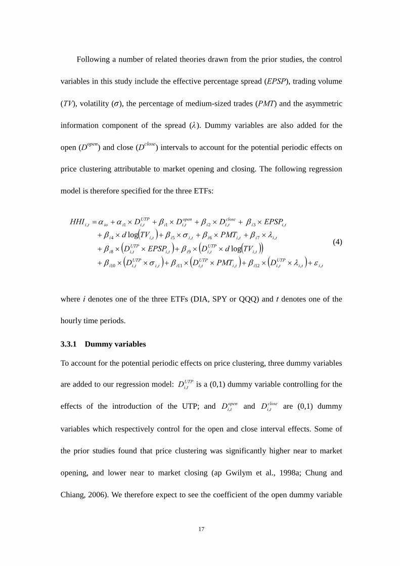
Following a number of related theories drawn from the prior studies, the control
variables in this study include the effective percentage spread (EPSP), trading volume
(TV), volatility (σ ), the percentage of medium-sized trades (PMT) and the asymmetric
information component of the spread (λ ). Dummy variables are also added for the
open (Dopen) and close (Dclose) intervals to account for the potential periodic effects on
price clustering attributable to market opening and closing. The following regression
model is therefore specified for the three ETFs:
( )( ) ( )( )( ) ( ) ( ) titi
UTPtiiti
UTPtiiti
UTPtii
tiUTP
tiitiUTP
tii
tiitiitiitii
tiiclosetii
opentii
UTPtiiioti
DPMTDD
TVdDEPSPD
PMTTVdEPSPDDDHHI
,,,12,,11,,10
,,9,,8
,7,6,5,4
,3,2,1,1,
log
log
ελββσβ
ββ
λββσββ
βββαα
+××+××+××+
××+××+
×+×+×+×+
×+×+×+×+=
(4)
where i denotes one of the three ETFs (DIA, SPY or QQQ) and t denotes one of the
hourly time periods.
3.3.1 Dummy variables
To account for the potential periodic effects on price clustering, three dummy variables
are added to our regression model: UTP
tiD , is a (0,1) dummy variable controlling for the
effects of the introduction of the UTP; and opentiD , and close
tiD , are (0,1) dummy
variables which respectively control for the open and close interval effects. Some of
the prior studies found that price clustering was significantly higher near to market
opening, and lower near to market closing (ap Gwilym et al., 1998a; Chung and
Chiang, 2006). We therefore expect to see the coefficient of the open dummy variable
18
having a positive value, and the coefficient of the close dummy variable having a
negative value. Furthermore, as argued by Boehmer and Boehmer (2003), the
coefficient of the UTP dummy variable is expected to be negative because of the
improvement in market liquidity.
3.3.2 Effective percentage spread
Traditionally, the quoted percentage spread ignores the effect of execution inside or
outside the quote; we therefore use the effective percentage spread (EPSPt) both as a
measure of trading costs and as a proxy for market liquidity. Following Huang and
Stoll (1994), we compute the effective percentage spread as follows:
t
ttt Q
QPEPSP
−=
2, (5)
where Pt is the trade price and Qt is the quote midpoint just prior to the trade. This
measure considers the effect of execution inside or outside the quote and can be used
as an approximation for the total price impact of a trade. Harris (1991) and Aitken et al.
(1996) argued that clustering is expected to increase during periods of high quoted
spread, since traders would be using much coarser discrete price sets; therefore, the
coefficient of the effective percentage spread is expected to be positive, which also
implies that less price clustering may occur in more liquid markets.
3.3.3 Trading volume
Many of the prior empirical studies on volume have used some form of de-trending to
induce stationarity; hence, we adjust the trading volume by using the log-linear

19
de-trending regression, i.e., ( )tTVd log ( )tTVlog= ( )tba ˆˆ +− , where d log(TVt) is the
log-linear de-trended volume at period t. By using the log-linear de-trended volume,
within which de-trending of the time-series properties of trading volume is taken into
consideration, we can avoid the problem of non-stationarity, thereby reflecting the
trading activities of the markets. Furthermore, since trading volume does reflect the
trading activities of the markets, we expect to obtain an output demonstrating a
reduction in clustering during periods of high trading volume, with the coefficient
expected to be negative, as argued by Harris (1991).
3.3.4 Volatility
The intraday hourly volatility (σt ) is calculated using the Rogers and Satchell (1991)
extreme value estimator, which simultaneously uses the high, low, opening and closing
prices, i.e.:
+
=
t
t
t
t
t
t
t
tt O
LCL
OH
CH
loglogloglogσ , (6)
where Ht , Lt , Ot and Ct denote the respective high, low, opening and closing prices
during time period t. Harris (1991) and Aitken et al. (1996) similarly argued that price
clustering was expected to increase during periods of high volatility; therefore, the
coefficient of volatility is also expected to be positive in our study.
3.3.5 Percentage of medium-sized trades
The percentage of medium-sized trades (PMTt) is calculated as the proportion of
medium-sized trades to total trades for each hourly interval. Consistent with Barclay

20
and Warner (1993), we define medium-sized trades as trades between 500 and 9,999
shares. Barclay and Warner (1993) and Chakravarty (2001) argued that if trading by
informed investors was the main cause of stock price changes, and if trading by
informed traders was also concentrated in trades of certain sizes, then most of a stock’s
cumulative price change should take place in medium-sized trades. Based on the
stealth-trading hypothesis, medium-sized trades can display disproportionately large
cumulative price changes relative to the overall proportion of their trades.
Ball et al. (1985) also contended that the degree of price resolution was dependent
on the amount of information in the market, the level of the price and its variability.
We expect to see price clustering decreasing with a high percentage of medium-sized
trades, essentially because of a fall in the extent of haziness for asset prices; therefore,
similar to the argument of Ball et al. (1985), the coefficient of percentage of
medium-sized trades in this study is also expected to be negative.
3.3.6 Asymmetric information component
The asymmetric information component (λt) is a compensatory factor arising from the
asymmetric information risk faced by liquidity suppliers. Our model of the asymmetric
information component of spread is based upon Lin et al. (1995):
1,,,1, ++ +=− titiititi eZQQ λ , (7)
1,,1, ++ += titiiti ZZ ηθ , (8)
where Qi ,t is the prevailing quote midpoint for a transaction in ETF i, at time t; Zi ,t is
the one-half signed effective spread, defined as the transaction price minus the
21
prevailing quote midpoint, with Zi ,t < 0 for a sell order, and Zi ,t > 0 for a buy order ; and
the disturbance terms ei ,t+1 and ηi ,t+1 are assumed to be uncorrelated. Since λt reflects
the quote revision in response to a trade as a fraction of the effective spread, it can be
viewed as the asymmetric information component of the effective spread. An
appropriate asymmetric information component must exist to compensate for this risk
of loss, such that liquidity providers can maintain their operations against informed
trading activities.
Widening the spread also reduces the potential losses to informed traders for
liquidity providers by ensuring that informed traders trade at less attractive prices.
According to the negotiation hypothesis, traders will use a fine set of prices when asset
values are well known; i.e., that there is little dispersion between trade reservation
prices. Thus, we speculate that a positive relationship exists between price clustering
and the asymmetric information component.
3.3.7 Interaction variables
Finally, we find that there were significant increases or decreases in the means of some
control variables after the introduction of UTP, which implies that the NYSE entry may
have brought about significant changes to these control variables. We therefore allow the
slope coefficients in this regression model to change with the introduction of the UTP
system. By utilizing the interaction terms in our regression model, we can display the
effects of the NYSE entry on the control variables. This specification is also similar to
the research methodology adopted in the study by Boehmer and Boehmer (2003).

22
Although the bid-ask spread is an important factor determining the overall extent
of clustering in Equation (4), some of the prior empirical studies have shown that price
clustering could also influence the bid-ask spread (ap Gwilym et al., 1998a; Hasbrouck,
1999). Hence, the bid-ask spread and the extent of clustering can be determined
simultaneously.
Similarly, we employ the Hausman (1978) specification test to test for potential
endogeneity in the effective percentage spread variable in Equation (4), with the
results indicating that the effective percentage spread is generally endogenous;
therefore, the models are estimated using the generalized method of moment (GMM)
approach, which uses the lagged effective percentage spread and average quoted depth
as the instrumental variables for the effective percentage spread.
We briefly explain here the GMM estimation method proposed in our study. Let zt
be the vector of the instrumental variables which include dummy variables for the
introduction of UTP, open and close intervals, log-linear de-trended volume, volatility,
the percentage of medium-sized trades, the asymmetric information component, the
quoted depth and the effective percentage spread at period t –1. The GMM estimator is
based largely on the moment conditions that:
( ) 0=ttzE ε (9)
where εt is the error term in Equation (4).6
We also use a multivariate regression approach to explore the impacts of various
6 A detailed explanation of the estimation procedure was provided by Hamilton (1994).
23
trading characteristic variables on the price clustering of ETFs following the entry of
the NYSE into the ETF markets. The empirical model is written as follows:
( )titiitiitii
tiitiiclosetii
opentiiiti
PMTβTVdEPSPDDHHI
,,7,6,5
,4,3,2,10,
log
ελββσββββα
+×+×+×+
×+×+×+×+= (10)
Equation (10) is also estimated by GMM if the effective percentage spread is
endogenous, with the definitions of the explanatory variables being the same as those in
Equation (4).
4. EMPIRICAL RESULTS
4.1 The Extent and Frequency of Price Clustering
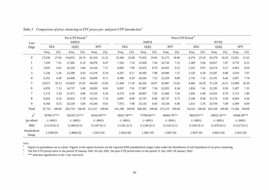
The frequency distribution of the last digit, the goodness-of-fit statistics, the HHI and the
standardized range of the prices of the three ETFs in the AMEX and the NYSE are
summarized in Table 3.7 The results show that for DIA prices in the AMEX, the last digit
0 appeared most frequently prior to the introduction of UTP, coming up in 27.66 per cent
of all trades. The last digit 5 was the next most likely to occur, appearing in about 20.13
per cent of all trades; however, none of the other possible last digits occurred with a
frequency of more than about 9 per cent. With the implementation of UTP, the frequency
of last digits 0 and 5 fell noticeably, with 0 appearing in only about 23.08 per cent of all
trades and 5 appearing in about 17.29 per cent of all trades; there was an increase in the
frequency of all other last digits, with the exceptions of last digits 1 and 9.
7 The cell frequencies are determined based upon the last digit, with goodness-of-fit statistics being constructed as the sum of the squared deviations of the cell frequencies from the expected frequency under the null hypothesis of uniform distribution (i.e., one-tenth). The Herfindahl-Hirschman index (HHI) and standardized range method are also used to test for price concentration.

24
< Table 3 is inserted about here >
For QQQ prices in the AMEX, Table 3 shows that prior to the introduction of UTP,
the frequency of the last digit 0 was 29.74 per cent, whilst the frequency of last digit 5
was 25.93 per cent; after the introduction of UTP, occurrences of the former were
reduced to 19.83 per cent, whilst the latter fell to 18.07 per cent. It is clear that the last
digit distribution in QQQ prices was far from uniform prior to the introduction of UTP,
given that the last digits 0 and 5 appeared in more than 55 per cent of all trading prices.
Furthermore, investors trading in the NYSE also demonstrated a slight preference for the
last digit 0, over the last digit 5, with the respective occurrence of these digits being
16.50 per cent and 14.15 per cent. All of the results of the goodness-of-fit statistics show
that the QQQ prices did not follow any uniform distribution.
For SPY prices, the results reveal that the greatest percentage of clustering in the
AMEX was demonstrated where the last digit was 0, with the price clustering for this
digit in the two sub-periods being 21.22 per cent prior to the UTP implementation, and
18.96 per cent afterwards. The next most likely last digit in the AMEX prior to the
introduction of UTP was 5, accounting for 15.94 per cent of all trades, whilst the
occurrences of other last digits varied between 6.19 per cent and 9.01 per cent. Price
clustering was still not uniform in the period after the introduction of UTP, with the
last digits 0 and 5 together accounting for 34.58 per cent of all reported trade prices in
the AMEX, and 38.02 per cent of all reported trade prices in the NYSE, as compared
to the expected 20 per cent.
25
The HHIs for the DIAs, QQQs and SPYs are also reported in Tables 3. Although
the expected HHI under the null hypothesis is 0.1, the HHIs for DIAs in the AMEX
were 0.1519 prior to the introduction of UTP, and 0.1281 afterwards, whereas the HHI
for DIAs in the NYSE was 0.1395. For QQQs traded in the NYSE, the estimated HHI
was 0.1076, slightly higher than its expected value of 0.1 under the null hypothesis,
whereas the respective HHIs for QQQs in the AMEX, prior to and after the
introduction of UTP, were 0.1804 and 0.1206. The HHI estimations for SPYs in the
AMEX, for the periods both before and after the introduction of UTP, were 0.1207 and
0.1145, respectively, whereas the HHI for SPYs in the NYSE was 0.1227.
Since the expected HHI value is 0.1 under no price clustering, there is no denying
that the prices of DIAs, QQQs and SPYs in the AMEX demonstrated a higher degree
of price concentration prior to the introduction of UTP. Furthermore, by comparing the
change before and after UTP implementation, the analysis seems to indicate that the
trading prices for the three regular ETFs became less centralized in the AMEX and the
NYSE after the introduction of UTP.
Very similar results are obtained in examining the standardized range. Those for
DIAs in the AMEX were 2.2399 prior to the introduction of UTP, and 1.6910
afterwards, whereas for DIAs in the NYSE the figure was 1.9927. The respective
standardized ranges for QQQs in the AMEX, prior to and after the introduction of UTP,
were 2.4868 and 1.3001, whereas the figure for QQQs in the NYSE was 0.8623.
Similarly, the respective standardized ranges for SPYs in the AMEX, prior to and after
26
the introduction of UTP, were 1.5031 and 1.2007, whereas the figure for SPYs in the
NYSE was 1.5631.
Our research results conclude that the prices of these three ETFs did not follow
uniform distribution, since the expected value of the standardized range is zero. The
results also show that the trading prices for the three regular ETFs became less
centralized in the AMEX and the NYSE after the introduction of UTP, with the
exception of SPYs in the NYSE.
To summarize, the existence of price clustering for the three ETFs is a
regularly-occurring phenomenon, whether this is examined in the pre-UTP AMEX, the
post-UTP AMEX or the NYSE. Additionally, the introduction of UTP seems to have led to
an obvious reduction in the occurrence of price clustering in the AMEX market, a result
which may be attributable to the fact that investors can easily switch trading exchanges, so
as to get their orders placed into the order book at the exchange which can offer accurate
prices; the UTP also allows traders to refine their resolution more easily.
This result leads us to conclude that the main reason for the lower severity of
price clustering in ETFs may be the market competition between the AMEX and the
NYSE. The observation in this study is consistent with the finding of Boehmer and
Boehmer (2003), that the NYSE entry led to a dramatic improvement in liquidity. This
finding implies that more liquid markets can reduce the occurrences of price clustering,
and that market competition may also facilitate a reduction in such occurrences, as
argued by Harris (1991) and Aitken et al. (1996).

27
4.2 Related Results on post-UTP Price Clustering
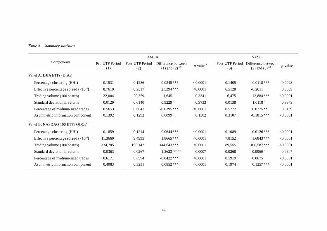
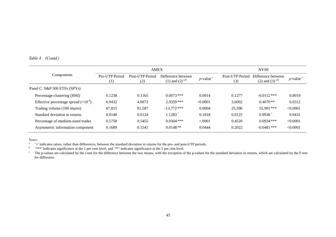
The summary statistics on the ETFs, in terms of daily average control variables for the
pre-UTP AMEX, post-UTP AMEX and NYSE entry, are presented in Table 4. The
control variables include the effective percentage spread calculated as 2|Pt – Qt |/Qt ,
where Pt is the trade price; Qt is the quote midpoint just prior to a trade; and trading
volume is the daily total volume. The standard deviation of return is used as a proxy
for volatility. The proportion of medium-sized trades to total trades is provided in
percentage terms, with medium-sized trades being defined as trades between 500 and
9,999 shares. The asymmetric information component of the spread is calculated using
the method proposed by Lin et al. (1995).8
< Table 4 is inserted about here >
The effective percentage spread, log-linear de-trended volume, standard deviation
of return, percentage of medium-sized trades and asymmetric information component
all changed significantly after UTP implementation. This result demonstrates that the
NYSE entry altered the market characteristics of the AMEX. We therefore explore
price clustering in the AMEX with the full model; that is, multiplying the interaction
explanatory variables by the UTP dummy variable, so as to accurately estimate the
effects of these variables on price clustering.
Similar to the results of Table 3, a significant reduction in the occurrences of
price clustering in the three ETFs is also revealed in Table 4 as a direct result of the
8 The Herfindahl-Hirschman index (HHI) is used to be a proxy for percentage clustering.
28
entry of the NYSE into the market. These results, which reveal reductions in both the
effective percentage spread and the asymmetric information component, are consistent
with the findings of Boehmer and Boehmer (2003).
4.2.1 Hausman specification test results
Table 5 presents the results of the Hausman specification test for the three ETFs. The test
is conducted to determine the endogeneity of the effective percentage spread in Equations
(4) and (10) by the addition of one extra explanatory variable within the equation; i.e., the
residuals from the regression of the effective percentage spreads on the set of
predetermined variables. The Hausman specification test is implemented as follows:
( )( )tiitiitii
tiitiitiiclosetii
opentii
UTPtiiiotiti
QDEPSP
PMTTVdDDDEPSPv
,81,7,6
,5,4,3,2,1,1,,
logˆˆˆ
ˆˆlogˆˆˆˆˆˆ
×+×+×+
×+×+×+×+×+×+−=
− ββλβ
βσββββαα
( )( ) tititiitii
tiitiitiitiiclosetii
opentii
UTPtiiioti
vQDbEPSPbbPMTbbTVdbDbDbDaaHHI
,,,81,7
,6,5,4,3,2,1,1,
ˆlog log
ερλσ
+×+×+×+
×+×+×+×+×+×+×+=
−
where DUTP is a (0,1) dummy variable controlling for the effect of the NYSE entry and
is excluded from Equation (10); Dopen and Dclose are (0,1) respective dummy variables
controlling for the open and close interval effects; dlog(TV) is the log-linear
de-trending hourly interval volume; σ is the intraday hourly volatility, calculated using
the Rogers and Satchell (1991) extreme value estimator; PMT is the percentage of
medium-sized trades; λ is the asymmetric information component of effective spreads;
EPSPt–1 is the lagged effective percentage spread; and log(QD) is the logarithm of the
quoted depth. The variable v̂ denotes the residuals from the effective percentage
29
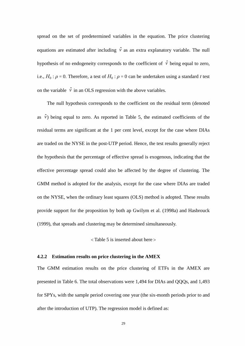
spread on the set of predetermined variables in the equation. The price clustering
equations are estimated after including v̂ as an extra explanatory variable. The null
hypothesis of no endogeneity corresponds to the coefficient of v̂ being equal to zero,
i.e., H0 : ρ = 0. Therefore, a test of H0 : ρ = 0 can be undertaken using a standard t test
on the variable v̂ in an OLS regression with the above variables.
The null hypothesis corresponds to the coefficient on the residual term (denoted
as v̂) being equal to zero. As reported in Table 5, the estimated coefficients of the
residual terms are significant at the 1 per cent level, except for the case where DIAs
are traded on the NYSE in the post-UTP period. Hence, the test results generally reject
the hypothesis that the percentage of effective spread is exogenous, indicating that the
effective percentage spread could also be affected by the degree of clustering. The
GMM method is adopted for the analysis, except for the case where DIAs are traded
on the NYSE, when the ordinary least squares (OLS) method is adopted. These results
provide support for the proposition by both ap Gwilym et al. (1998a) and Hasbrouck
(1999), that spreads and clustering may be determined simultaneously.
< Table 5 is inserted about here >
4.2.2 Estimation results on price clustering in the AMEX
The GMM estimation results on the price clustering of ETFs in the AMEX are
presented in Table 6. The total observations were 1,494 for DIAs and QQQs, and 1,493
for SPYs, with the sample period covering one year (the six-month periods prior to and
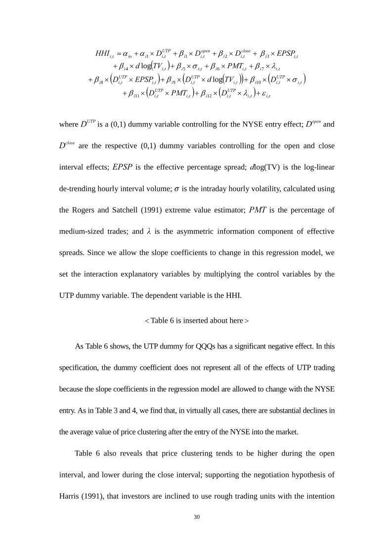
after the introduction of UTP). The regression model is defined as:
30
( )( ) ( )( ) ( )
( ) ( ) titiUTP
tiitiUTP
tii
tiUTP
tiitiUTP
tiitiUTP
tii
tiitiitiitii
tiiclosetii
opentii
UTPtiiioti
DPMTD
DTVdDEPSPD
PMTTVdEPSPDDDHHI
,,,12,,11
,,10,,9,,8
,7,6,5,4
,3,2,1,1,
log
log
ελββ
σβββ
λββσβββββαα
+××+××+
××+××+××+
×+×+×+×+
×+×+×+×+=
where DUTP is a (0,1) dummy variable controlling for the NYSE entry effect; Dopen and
Dclose are the respective (0,1) dummy variables controlling for the open and close
interval effects; EPSP is the effective percentage spread; dlog(TV) is the log-linear
de-trending hourly interval volume; σ is the intraday hourly volatility, calculated using
the Rogers and Satchell (1991) extreme value estimator; PMT is the percentage of
medium-sized trades; and λ is the asymmetric information component of effective
spreads. Since we allow the slope coefficients to change in this regression model, we
set the interaction explanatory variables by multiplying the control variables by the
UTP dummy variable. The dependent variable is the HHI.
< Table 6 is inserted about here >
As Table 6 shows, the UTP dummy for QQQs has a significant negative effect. In this
specification, the dummy coefficient does not represent all of the effects of UTP trading
because the slope coefficients in the regression model are allowed to change with the NYSE
entry. As in Table 3 and 4, we find that, in virtually all cases, there are substantial declines in
the average value of price clustering after the entry of the NYSE into the market.
Table 6 also reveals that price clustering tends to be higher during the open
interval, and lower during the close interval; supporting the negotiation hypothesis of
Harris (1991), that investors are inclined to use rough trading units with the intention
31
of reducing negotiation costs. Furthermore, since the coefficients of the effective
percentage spread were 0.1009 for DIAs, 0.0742 for QQQs and 0.1130 for SPYs, they
were all significantly positive and consistent with the findings of Ikenberry and
Weston (2005), which suggests that the spread appears to have significant and
consistent impacts on price clustering.
In addition, the relationship between price clustering and the log-linear de-trended
volume for the three ETFs appears to be insignificant. Specifically, we find that the
influence of the percentage of medium-sized trades on price clustering was in the
opposite direction. In the study by Chakravarty (2001), it was noted that medium-sized
investors have more information on the overall process of price changing; thus, we argue
that this would reduce the occurrences of clustering as a result of the prices being quoted
with less haziness. This result also provides support for the price resolution hypothesis.
Furthermore, the coefficients of the asymmetric information component were all
significantly positive for the three ETFs. With values of 0.0347, 0.1460 and 0.0667, it
is clear that information asymmetry may induce the occurrence of price clustering.
Thus, we argue that the asymmetric information component is an important
characteristic of price clustering in explaining the negotiation hypothesis.
As regards the entry of the NYSE into ETF trading, this may have resulted in
changing the sensitivity of ‘trading cost to order’ characteristics; such an effect is clear,
particularly where the pre-UTP market is less competitive. We further explore this
issue with the interaction explanatory variables by multiplying the control variables by

32
the UTP dummy variable. The results in Table 6 show that the coefficients of the
interaction terms in the effective percentage spread and asymmetric information
component were negative, whilst the coefficient of the interaction term in the
percentage of medium-sized trades was positive.
We can determine that all of the significant interaction terms had the opposite sign to
the pre-UTP coefficient, with most of them being smaller than the underlying coefficient.
For example, a single unit increase in the effective percentage spread of the DIA had the
effect of raising price clustering by 0.1009 prior to UTP trading, but by only 0.0623
(0.1009-0.0386) afterwards. This implies that the entry of the NYSE significantly reduced
the effects on price clustering from the effective percentage spread, the percentage of
medium-sized trades and the asymmetric information component; that is, the entry of the
NYSE led to dramatic changes in the market characteristics of the AMEX.
Our results provide additional support for the argument of Chowdhry and Nanda
(1991), that competition for market making services induces market makers to take
action, such as ensuring that price information is made public, thereby deterring
informed trading; that is, the influence of medium-sized trades on price clustering was
reduced as a result of the entry of the NYSE. Based on the price resolution hypothesis,
this finding implies that information on price changes in medium-sized trades may be
available in advance as a result of the competition between the AMEX and the NYSE,
and this could well have been responsible for the reduction in the asymmetric
information component after the entry of the NYSE.
33
In summary, our results indicate that the introduction of UTP was responsible for
producing a more liquid market. If the main reason for potential price clustering is the
quotation behavior of liquidity providers, the reduction in price clustering after the
entry of the NYSE may have been attributable to a smaller asymmetric information
component as a direct result of the improvement in market liquidity. In other words,
traders will use a finer set of prices when the dispersion existing between trade
reservation prices becomes small, resulting in a reduction in price clustering in the
post-UTP period. This causality between price clustering and market liquidity, as
argued by the negotiation hypothesis, can be illustrated more clearly through our
analysis of the changes in the asymmetric information component.
4.2.3 Estimation results of price clustering in the NYSE
The coefficient estimates of the price clustering regression are shown in Table 7, using
the GMM method for QQQs and SPYs on the NYSE, and the OLS method for DIAs.
The overall sample period for the three ETFs in the AMEX covers the six-month
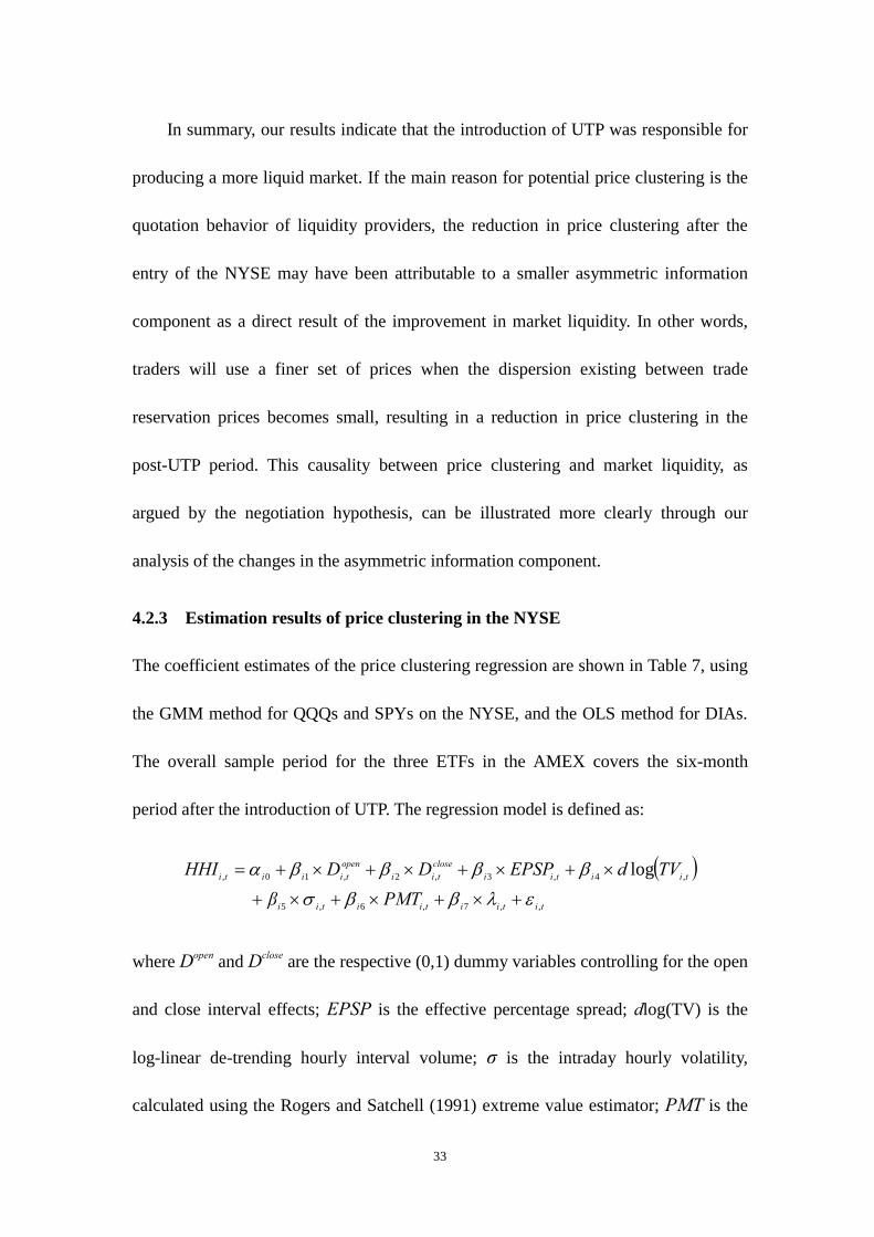
period after the introduction of UTP. The regression model is defined as:
( )titiitiitii
tiitiiclosetii
opentiiiti
PMTβTVdEPSPDDHHI
,,7,6,5
,4,3,2,10,
log
ελββσββββα
+×+×+×+
×+×+×+×+=
where Dopen and Dclose are the respective (0,1) dummy variables controlling for the open
and close interval effects; EPSP is the effective percentage spread; dlog(TV) is the
log-linear de-trending hourly interval volume; σ is the intraday hourly volatility,
calculated using the Rogers and Satchell (1991) extreme value estimator; PMT is the
34
percentage of medium-sized trades; and λ is the asymmetric information component of
the effective spreads. Since the results of the Hausman specification test for trading in
DIAs on the NYSE were insignificant, we estimate the regression on price clustering
using the OLS method. The sample sizes were 731 DIAs, 734 QQQs and 734 SPYs,
with the sample period covering the six-month period after the entry of the NYSE into
AMEX-listed ETF trading.
The results indicate that price clustering appears to be higher during the open
interval, and lower during the close interval, which is consistent with the findings of ap
Gwilym (1998a) and Chung and Chiang (2006). Furthermore, the coefficients of the
effective percentage spread on the three ETFs were all significantly positive. With
values of 0.0891, 0.0054 and 0.2783, this clearly suggests that the existence of spread
has a detrimental effect on clustering. As to the variable ‘the percentage of
medium-sized trades’, the effect was significantly negative, which also supports the
price resolution hypothesis.
< Table 7 is inserted about here >
The coefficients of the asymmetric information component, which were
significant positively, were 0.0246 for QQQs and 0.0186 for SPYs, suggesting that
higher information asymmetry significantly raises the potential for price clustering.
Within the NYSE market, the phenomenon of price clustering was, on the whole,
obviously influenced by market liquidity, a finding which is similar to the results on
the AMEX market reported in Table 6.

35
5. CONCLUSIONS
This paper has examined the impact of price clustering following the entry of the NYSE
into AMEX-listed ETF trading. By exploring the three most active ETFs (DIAs, QQQs
and SPYs) on the AMEX and NYSE, we have attempted to examine whether the
implementation of multi-market trading affected the occurrence of price clustering
through the causality stated in the theoretical hypotheses. The results indicate that price
clustering in the AMEX fell after UTP implementation. The results also show that
trading characteristic variables, such as the effective percentage spread, the percentage
of medium-sized trades and the asymmetric information component, could well explain
the change in price clustering. These relationships appear consistent with the arguments
of the price resolution and negotiation hypotheses. Moreover, from our examination of
the interaction terms in our empirical models, the existence of an NYSE entry effect is
discernible on market structure, because there were changes in the direction and
magnitude of all the coefficients of the significant control variables; that is, the market
characteristics of the AMEX obviously changed as a result of UTP implementation.
The abatement of price clustering after the entry of the NYSE into the market
may have resulted from the increased market competition leading to the elimination of
asymmetric information and a dramatic improvement in market liquidity. These results
find support in a number of prior studies (Harris, 1991; Grossman et al., 1997;
Martinez and Tse, 2006) which reported higher price clustering in less liquid markets.
Considering the quotation behavior of liquidity providers as a major potential cause of
36
price clustering, the reduction in price clustering after the NYSE entry may be
attributable to a reduction in the asymmetric information component as a result of the
improvements in market liquidity. This causality between price clustering and market
liquidity, as argued in the negotiation hypothesis, is illustrated most clearly by the
changes in the asymmetric information component.
Our results also indicate that the percentage of medium-sized trades affects price
clustering in a significantly opposite direction, but that the relationship abated after the
entry of the NYSE into the ETF markets. This result provides support for the price
resolution hypothesis and implies that information on price changes may be available
in advance because of the competition between the AMEX and the NYSE. Therefore,
based on the price resolution hypothesis, as a direct result of UTP implementation, as
argued by Chowdhry and Nanda (1991), pricing information was made public.
In conclusion, the findings of this study have implications on the relationship
between multi-market trading and price clustering. More specifically, our results
support the main tenets of the price resolution and negotiation hypotheses. The overall
findings suggest that the introduction of the UTP system contributed to a reduction in
price clustering, a result which may be attributable to the improvement in market
liquidity and the continuity in quoted prices through a reduction in the asymmetric
information component. Moreover, making price information public, and thereby
alleviating insider trading, may also provide feasible explanations for the changes
following the introduction of UTP into the ETF markets.

37
REFERENCES
Aitken, M., P. Brown, C. Buckland, H.Y. Izan and T. Walter (1996), ‘Price Clustering
on the Australian Stock Exchange’, Pacific-Basin Finance Journal, 4: 297-314.
ap Gwilym, O. and E. Alibo (2003), ‘Decreased Price Clustering in FTSE 100 Futures
Contracts following the Transfer from Floor to Electronic Trading’, Journal of
Futures Markets, 23: 647-59.
ap Gwilym, O., A. Clare and S. Thomas (1998a), ‘Extreme Price Clustering in the
London Equity Index Futures and Options Markets’, Journal of Banking and
Finance, 22: 1193-206.
ap Gwilym, O., A. Clare and S. Thomas (1998b), ‘Price Clustering and Bid-Ask
Spreads in International Bond Futures’, Journal of International Financial
Markets, Institutions and Money, 8: 377-91.
Ball, C.A., W. Torous and A.E. Tschoegl (1985), ‘The Degree of Price Resolution: The
Case of the Gold Market’, Journal of Futures Markets, 5: 29-43.
Barclay, M.J. (1997), ‘Bid-Ask Spreads and the Avoidance of Odd-eighth Quotes on
the NASDAQ: An Examination of Exchange Listing’, Journal of Financial
Economics, 45: 35-60.
Barclay, M.J. and J.B. Warner (1993), ‘Stealth and Volatility: Which Trades Move
Prices?’, Journal of Financial Economics, 34: 281-306.
Bessembinder, H. (1997), ‘The Degree of Price Resolution and Equity Trading Costs’,
Journal of Financial Economics, 45: 9-34.
Boehmer, B. and E. Boehmer (2003), ‘Trading your Neighbor’s ETFs: Competition or
Fragmentation?’, Journal of Banking and Finance, 27: 1667-703.
Brown, P., A. Chua and J. Mitchell (2002), ‘The Influence of Cultural Factors on Price
Clustering: Evidence from Asia-Pacific Stock Markets’, Pacific-Basin Finance
Journal, 10: 307-22.
Chakravarty, S. (2001), ‘Stealth-trading: Which Traders’ Trades Move Stock Prices?’,
Journal of Financial Economics, 61: 289-307.

38
Chowdhry, B. and V. Nanda (1991), ‘Multi-market Trading and Market Liquidity’,
Review of Financial Studies, 4: 483-511.
Christie, W.G. and P.H. Schultz (1994), ‘Why do NASDAQ Market Makers Avoid
Odd-eighth Quotes?’, Journal of Finance, 49: 1813-40.
Christie, W.G.., J.H. Harris and P.H. Schultz (1994), ‘Why did NASDAQ Market
Makers Stop Avoiding Odd-eighth Quotes?’, Journal of Finance, 49: 1841-60.
Chung, H. and S. Chiang (2006), ‘Price Clustering in E-mini and Floor-traded Index
Futures’, Journal of Futures Markets, 26: 269-96.
Cooney, J., B.F. Van Ness and R.A. Van Ness (2003), ‘Do Investors Prefer Even-eighth
Prices? Evidence from NYSE Limit Orders’, Journal of Banking and Finance, 27:
719-48.
Goodhart, C. and R. Curcio (1991), ‘The Clustering of Bid-Ask Prices and Spread in
the Foreign Exchange Markets’, Discussion Paper No.110, London: London
School of Economics, Financial Markets Group.
Grossman, S.J., M.H. Miller, K.R. Cone, D.R. Fischel and D.J. Ross (1997),
‘Clustering and Competition in Asset Markets’, Journal of Law and Economics,
40: 23-60.
Hameed, A. and E. Terry (1998), ‘The Effect of Tick Size on Price Clustering and
Trading Volume’, Journal of Business Finance and Accounting, 25: 849-67.
Hamilton, J.D. (1994), Time Series Analysis, Princeton, New Jersey: Princeton
University Press.
Harris, L. (1991), ‘Stock Price Clustering and Discreteness’, Review of Financial
Studies, 4: 389-415.
Hasbrouck, J. (1999), ‘Security Bid-Ask Dynamics with Discreteness and Clustering:
Simple Strategies for Modeling and Estimation’, Journal of Financial Markets, 2:
1-28.
Hausman, J.A. (1978), ‘Specification Tests in Econometrics’, Econometrica, 46:
1251-71.

39
Hornick, J., J. Cherianand and D. Zakay (1994), ‘The Influence of Prototypic Values
on the Validity of Studies using Time Estimates’, Journal of Market Research
Society, 36: 145-7.
Huang, R.D. and H.R. Stoll (1994), ‘Market Microstructure and Stock Return
Predictions’, Review of Financial Studies, 7: 179-213.
Huang, R.D. and H.R. Stoll (1996), ‘Dealer versus Auction Markets: A Paired
Comparison of Execution Costs on the NASDAQ and the NYSE’, Journal of
Financial Economics, 41: 313-57.
Ikenberry, D. and J.P. Weston (2005), ‘Clustering in US Stock Prices after
Decimalization’, Working Paper, Urbana-Champaign and Houston: University of
Illinois at Urbana-Champaign and Rice University.
Kahneman, D., P. Slovic and A. Tversky (1982), Judgment under Uncertainty:
Heuristic and Biases, New York: Cambridge University Press.
Kandel, S., O. Saring and A. Wohl (2001), ‘Do Investors Prefer Round Stock Prices?
Evidence from Israeli IPO Auctions’, Journal of Banking and Finance, 25: 1543-51.
Khan, W.A. and H.K. Baker (1993), ‘Unlisted Trading Privileges, Liquidity and Stock
Returns’, Journal of Financial Research, 16: 221-36.
Lin, J.C., G.C. Sanger and G.G. Booth (1995), ‘Trade Size and Components of the
Bid-Ask Spread’, Review of Financial Studies, 8: 1153-83.
Loomes, G. (1988), ‘Different Experimental Procedures for Obtaining Valuations of
Risky Actions: Implications for Utility Theory’, Theory and Decision, 25: 1-23.
Martinez, V., and Y. Tse (2006), ‘Multi-market Trading in the Gold Futures Market’,
Working paper, University of Texas, San Antonio.
Ohta, W. (2006), ‘An Analysis of Intra-day Patterns in Price Clustering on the Tokyo
Stock Exchange’, Journal of Banking and Finance, 30: 1023-39.
Osler, C.L. (2003), ‘Currency Orders and Exchange Rate Dynamics: An Explanation
for the Predictive Success of Technical Analysis’, Journal of Finance, 58:
1791-1820.

40
Rogers, L.C.G. and S.E. Satchell (1991), ‘Estimating Variance from High, Low and
Closing Prices’, Annuals of Applied Probability, 1: 504-12.
Schwartz, A., B.F. Van Ness and R.A. Van Ness (2004), ‘Clustering in the Futures
Markets: Evidence from S&P 500 Futures Contracts’, Journal of Futures Markets,
24: 413-28.
Tse, Y. and G. Erenburg (2003), ‘Competition for Order Flow, Market Quality and
Price Discovery in the NASDAQ-100 Index Tracking Stock’, Journal of
Financial Research, 26: 301-18.
Tse, Y. and T. Zabotina (2001), ‘Transaction Costs and Market Quality: Open-outcry
versus Electronic Trading’, Journal of Futures Markets, 21: 713-35.
Tversky, A. and D. Kahneman (1974), ‘Judgment under Uncertainty: Heuristics and
Biases’, Science, 185: 1124-31.
Weston, J.P. (2000), ‘Competition on the NASDAQ and the Impact of Recent Market
Reforms’, Journal of Finance, 55: 2265-98.
Yeoman, J.C. (2001), ‘The Optimal Spread and Offering Price for Underwritten
Securities’, Journal of Financial Economics, 62: 169-98.

41
Table 1 Variables and results of prior studies on price clustering
Panel A: Vertical-sectional Studies Panel B: Panel Study
ap Gwilym (1998)
Schwartz et al. (2004)
Chung and Chiang (2006)
Ohta (2006)
Variables LIFFE CME
CME/CBOT Floor-traded
CME/CBOT E-mini
TOYKO Continuous
Auction
TOYKOCall
Auction
Open + + + Close – – – Trade size – – + + Price . Number of trades – – Return + + . Spread + + + Tick volume + – Std. Dev. in Price + + + Open interest – Back-month contract + E-mini introduction + Contract redesign – Firm size – – Volatility + . Relative tick size – – Morning opening +
Panel C: Cross-sectional Studies Harris (1991)
Christie and Schultz (1994)
Aitken et al. (1996)
Ikenberry and Weston (2005)
Cooney et al. (2003) Variables
NYSE/ AMEX NASDAQ ASX NASDAQ
/NYSE NYSE early limit orders
NYSE daylimit orders
Trade size . + Price + + + + + + Number of trades + – + . + Spread + Std. Dev. in Price + + . Firm size – . . – . . Volatility + + + + . Institutional ownership + Closed-end funds – – – OTC market + Number of dealers . Listed options . – Dual listed . Odd-eighths used – Market volatility + Buyer-initiated + Resource stock . Short selling –
Note: The symbols are as follows: ‘+’ indicates positive and significant; ‘–’ indicates negative and significant; and
‘·’ indicates no effect.
42
Table 2 Factors involved in price clustering
Factors Variables
Haziness Price
ResolutionNegotiation
Costs Informed
TraderPrice
DiscoveryQuotation
Habit Other
Factors
Open
Close a
Trade size
Price
Number of trades b
Return
Spread
Tick volume c
Std. Dev. in Price
Firm size
Volatility d
Institutional ownership
Closed-end funds
OTC market
Listed options e,f
Odd-eighths Used
Market volatility
Buyer-initiated
Resource stock
Short selling
Open interest
Back-month contract
E-mini introduction
Contract redesign g
Notes: a Decrease in desired spread. b Increase in value uncertainty. c Market will be active. d Plentiful reservation price. e Short selling limit exceeded. f Informed trading with low cost. g Decrease in tick size.
43
Table 3 Comparison of price clustering in ETF prices pre- and post-UTP introduction a
Pre-UTP Period b Post-UTP Period b
AMEX AMEX NYSE DIA QQQ SPY DIA QQQ SPY DIA QQQ SPY
Last Digit
Freq. (%) Freq. (%) Freq. (%) Freq. (%) Freq. (%) Freq. (%) Freq. (%) Freq. (%) Freq. (%)
0 27,039 27.66 134,055 29.74 45,318 21.22 23,360 23.08 73,052 19.83 52,172 18.96 6,276 25.59 43,278 16.50 15,851 21.63
1 7,439 7.61 27,482 6.10 18,078 8.47 7,182 7.10 25,928 7.04 20,726 7.53 1,389 5.66 20,657 7.87 4,770 6.51
2 5,876 6.01 26,336 5.84 16,164 7.57 8,085 7.99 32,052 8.70 26,265 9.55 2,201 8.97 24,574 9.37 6,963 9.50
3 5,144 5.26 22,208 4.93 13,218 6.19 6,247 6.17 29,385 7.98 20,840 7.57 1,520 6.20 23,297 8.88 5,619 7.67
4 6,252 6.40 24,468 5.43 18,609 8.71 8,386 8.29 26,643 7.23 22,259 8.09 1,756 7.16 22,191 8.46 5,697 7.78
5 19,673 20.13 116,859 25.93 34,039 15.94 17,494 17.29 66,565 18.07 42,987 15.62 4,484 18.28 37,129 14.15 12,008 16.39
6 6,970 7.13 24,737 5.49 18,820 8.81 8,007 7.91 27,907 7.58 22,935 8.34 1,826 7.45 22,295 8.50 5,387 7.35
7 5,174 5.29 21,973 4.88 13,535 6.34 6,374 6.30 28,907 7.85 21,060 7.65 1,492 6.08 23,033 8.78 5,713 7.80
8 6,024 6.16 26,053 5.78 16,532 7.74 8,091 8.00 32,797 8.90 26,737 9.72 2,168 8.84 25,170 9.59 6,859 9.36
9 8,160 8.35 26,539 5.89 19,244 9.01 7,972 7.88 25,156 6.83 19,138 6.96 1,413 5.76 20,704 7.89 4,399 6.00
Total 97,751 100.00 450,710 100.00 213,557 100.00 101,198 100.00 368,392 100.00 275,119 100.00 24,525 100.00 262,328 100.00 73,266 100.00
χ2 50766.57*** 362347.21*** 44102.60*** 28427.58*** 75789.64*** 40004.78*** 9692.83*** 20032.34*** 16648.38***
(p-value) (<.0001) (<.0001) (<.0001) (<.0001) (<.0001) (<.0001) (<.0001) (<.0001) (<.0001)
HHI 0.1519 [0.1] 0.1804 [0.1] 0.1207 [0.1] 0.1281 [0.1] 0.1206 [0.1] 0.1145 [0.1] 0.1395 [0.1] 0.1076 [0.1] 0.1227 [0.1]
Standardized Range
2.2399 [0] 2.4868 [0] 1.5031 [0] 1.6910 [0] 1.3001 [0] 1.2007 [0] 1.9927 [0] 0.8623 [0] 1.5631 [0]
Note: a Figures in parentheses are p-values. Figures in the square brackets are the expected HHI (standardized range) value under the distribution of null hypothesis of no price clustering. b The Pre-UTP period refers to the period 29 January 2001-30 July 2001; the post-UTP period refers to the period 31 July 2001-30 January 2002. c *** indicates significance at the 1 per cent level.
44
Table 4 Summary statistics
AMEX NYSE Components Pre-UTP Period
(1) Post-UTP Period
(2) Difference between
(1) and (2) a,b p-value c Post-UTP Period (3)
Difference between(2) and (3) a,b p-value c
Panel A: DJIA ETFs (DIAs)
Percentage clustering (HHI) 0.1531 0.1286 0.0245 *** <0.0001 0.1405 -0.0118 *** 0.0023
Effective percentage spread (×10-4) 8.7610 6.2317 2.5294 *** <0.0001 6.5128 -0.2811 0.3859
Trading volume (100 shares) 22,004 20,359 1,645 0.3341 6,475 13,884 *** <0.0001
Standard deviation in returns 0.0129 0.0140 0.9229 + 0.3733 0.0138 1.0118 + 0.8973
Percentage of medium-sized trades 0.5653 0.6047 -0.0395 *** <0.0001 0.5772 0.0275 ** 0.0109 Asymmetric information component 0.1392 0.1292 0.0099 0.1302 0.3107 -0.1815 *** <0.0001
Panel B: NASDAQ 100 ETFs QQQs)
Percentage clustering (HHI) 0.1859 0.1214 0.0644 *** <0.0001 0.1089 0.0126 *** <0.0001
Effective percentage spread (×10-4) 11.3660 9.4995 1.8665 *** <0.0001 7.8152 1.6843 *** <0.0001
Trading volume (100 shares) 334,785 190,142 144,643 *** <0.0001 89,555 100,587 *** <0.0001
Standard deviation in returns 0.0363 0.0267 1.3623 +,*** 0.0007 0.0268 0.9960 + 0.9647
Percentage of medium-sized trades 0.6171 0.6594 -0.0422 *** <0.0001 0.5919 0.0675 <0.0001 Asymmetric information component 0.4083 0.3231 0.0852 *** <0.0001 0.1974 0.1257 *** <0.0001
45
Table 4 (Contd.)
AMEX NYSE Components Pre-UTP Period
(1) Post-UTP Period
(2) Difference between
(1) and (2) a,b p-value c Post-UTP Period (3)
Difference between(2) and (3) a,b p-value c
Panel C: S&P 500 ETFs (SPYs)
Percentage clustering (HHI) 0.1238 0.1165 0.0073 *** 0.0014 0.1277 -0.0112 *** 0.0019 Effective percentage spread (×10-4) 6.9432 4.0073 2.9359 *** <0.0001 3.6002 0.4070 ** 0.0312 Trading volume (100 shares) 67,815 81,587 -13,772 *** 0.0004 25,596 55,991 *** <0.0001 Standard deviation in returns 0.0140 0.0124 1.1283 + 0.1818 0.0125 0.9936 + 0.9431 Percentage of medium-sized trades 0.5758 0.5455 0.0304 *** <.0001 0.4520 0.0934 *** <0.0001 Asymmetric information component 0.1689 0.1541 0.0148 ** 0.0444 0.2022 -0.0481 *** <0.0001
Notes: a ‘+’ indicates ratios, rather than differences, between the standard deviation in returns for the pre- and post-UTP periods. b ‘***’ indicates significance at the 1 per cent level; and ‘**’ indicates significance at the 5 per cent level.
c The p-values are calculated by the t-test for the difference between the two means, with the exception of the p-values for the standard deviation in returns, which are calculated by the F-test for difference.

46
Table 5 Hausman specification test results for the three ETFs
Estimated coefficient of v̂
DIA QQQ SPY
Estimate p-value Estimate p-value Estimate p-value
AMEX -0.0145* 0.0897 -0.0259*** <0.0001 -0.0255*** <0.0001
NYSE -0.0152 0.4746 0.0084** 0.0117 -0.1384*** <0.0001 Note: ‘***’ indicates significance at the 1 per cent level; ‘**’ indicates significance at the 5 per cent level; and
‘*’ indicates significance at the 10 per cent level. Table 6 Estimation results of price clustering for the three ETFs on the AMEX
DIA QQQ SPY Variables
Estimate p-value Estimate p-value Estimate p-value
Constant 0.1051 *** <0.0001 0.1936 *** <0.0001 0.0628 *** <0.0001
DUTP -0.0128 0.4367 -0.0789 *** 0.0037 0.0113 0.3492
Dopen 0.0113 *** <0.0001 0.0087 *** 0.0002 -0.0018 0.2525
Dclose -0.0051 ** 0.0104 -0.0033 0.1376 -0.0047 *** 0.0018
EPSP 0.1009 *** <0.0001 0.0742 *** 0.0001 0.1130 *** <0.0001
d log(TV) -0.0035 0.1285 0.0003 0.9343 0.0024 * 0.0893
σ 0.0071 0.4707 0.0172 0.1886 -0.0145 0.2605
PMT -0.0653 *** 0.0021 -0.2684 *** <0.0001 -0.0278 ** 0.0208
λ 0.0347 * 0.0703 0.1460 *** <0.0001 0.0667 *** 0.0051
DUTP x EPSP -0.0386 *** 0.0027 -0.0501 ** 0.0149 -0.0538 *** 0.0014
DUTP x d log(TV) -0.0024 0.3438 0.0015 0.6571 0.0006 0.7290
DUTP x σ 0.0085 0.4735 -0.0158 0.2341 0.0191 0.1880
DUTP x PMT 0.0695 *** 0.0027 0.2295 *** <0.0001 0.0721 *** <0.0001
DUTP x λ -0.0365 * 0.0863 -0.1080 *** <0.0001 -0.0827 *** 0.0004
Note: ‘***’ indicates significance at the 1 per cent level; ‘**’ indicates significance at the 5 per cent level; and
‘*’ indicates significance at the 10 per cent level.

47
Table 7 Estimation results of price clustering for the three ETFs on the NYSE
DIA QQQ SPY Variables
Estimate p-value Estimate p-value Estimate p-value
Constant 0.1635 *** <0.0001 0.1107 *** <0.0001 0.0534 *** 0.0002
Dopen -0.0087 0.1974 0.0019 ** 0.0199 -0.0063 * 0.0835
Dclose -0.0143 ** 0.0342 -0.0030 *** 0.0008 -0.0077 * 0.0770
EPSP 0.0891 *** <0.0001 0.0054 * 0.0816 0.2783 *** <0.0001
d log(TV) -0.0117 *** <0.0001 -0.0008 0.5079 -0.0040 ** 0.0244
σ -0.0240 ** 0.0494 -0.0007 0.6548 -0.0150 0.5934
PMT -0.0466 *** 0.0012 -0.0084 * 0.0946 -0.0108 0.2975
λ 0.0184 0.1758 0.0246 *** <0.0001 0.0186 ** 0.0492
Note: ‘***’ indicates significance at the 1 per cent level; ‘**’ indicates significance at the 5 per cent level; and ‘*’ indicates significance at the 10 per cent level.
Recommended