i

MANUAL FOR FATIGUE ANALYSIS

OF

REINFORCED CONCRETE STRUCTURAL

ELEMENTS USING

VecTor2

Benard Isojeh

Frank Vecchio

December, 2017

ii

Abstract

The approach for the high-cycle fatigue life prediction of a reinforced concrete structural element

using VecTor2 nonlinear finite element analysis is presented. Mechanisms governing fatigue

damage progressions are briefly discussed, and the implementation of the models that account

for these mechanisms in VecTor2 software is treated subsequently. In addition, an illustrative

solution for a single element subjected to shear fatigue loading is given. The VecTor2 nonlinear

finite element analysis software, which incorporates fatigue damage models, allows for the

prediction of the fatigue residual capacity of an element after a given number of loading cycles.

The prediction of the instance at which steel reinforcement will fracture can also be obtained

from the analyses results.

iii

Table of contents

Abstract ………………………………………………………………………………………….... ii

List of Figures……………………………………………………………………………………....v

Notations…………………………………………………………………………………………..vii

CHAPTER 1: FATIGUE DAMAGE MECHANISMS…..……………………………….………..1

1.1 Introduction ……………………………………………………………………………….…....1

1.1.1Strength Degradation....……………………………………………………………….......1

1.1.2 Irreversible Strain Accumulation…………………………………………………………3

1.1.3 Reinforcement Crack Growth………………………………………………………….....4

1.2 Damage Constitutive Models for Residual Strength of Concrete……………………………....6

1.2.1 Normal Strength Concrete……………........................................………………………....6

1.2.2 High Strength Concrete……………………………………………………………………8

CHAPTER 2: IMPLEMENTATION OF DAMAGE MODELS IN DSFM…………………...…..9

2.1 Disturbed Stress Field Model……………………………………………………………….......9

2.1.1 Equilibrium Conditions……………………………………………………………….…...9

2.1.1.1 Equilibrium of Stresses at a Crack……………………………………………….....10

2.1.2 Compatibility Condition……………………………………………………………….…12

2.1.3 Constitutive Relation…………………………………………………………………….…..13

2.1.3.1 Concrete Constitutive Model…………………………………………………………..13

2.1.3.2 Conventional Reinforcement…………………………………………………………..17

CHAPTER 3: FINITE ELEMENT IMPLEMENTATION…………………………………….....18

3.1 Formulation……………………………………………………………………………………18

iv

3.2 Failure Criterion for Reinforced Concrete and Steel-Fibre Concrete under Fatigue

Loading……………………………………………………………………………………………22

3.3 Solution for Fatigue Loading at 10 000 cycles……………………………………………......24

CHAPTER 4: USE OF VecTor2 FOR FATIGUE DAMAGE ANALYSIS……………………...30

4.1 Defining Concrete Materials………………………………………………………………….30

4.2 Defining Reinforcement Properties……………………………………………………….…..31

4.3 Bond Types………………………………………………………………………………..….32

4.4 Structure and Mesh Definition…………………………………………………………….….33

4.5 Load Application under Fatigue Loading……………………………………………….…….33

4.6 Job Definition………………………………………………………………………………....34

4.7 Defining Fatigue Loading Parameters in Job………………………………………………....36

4.8 Solved Example…………………………………………………………………………….....38

5.0 SUMMARY AND RECOMMENDATION…………………………………………………..41

5.1 Summary………………………………………………………………………………………41

5.2 Recommendation……………………………………………………………………………...41

6.0 REFERENCES……………………………………………………………………………......42

v

List of Figures

CHAPTER 1: FATIGUE DAMAGE MECHANISMS

Fig. 1.1 – Estimation of damage parameter s………………………………………………………...2

Fig. 1.2 – Crack growth on a reinforcing bar cross section…………………………………………5

Fig. 1.3 - Modified Stress-strain curve for damaged concrete……………………………………...7

CHAPTER 2: IMPLEMENTATION OF DAMAGE MODELS IN DSFM

Fig. 2.1 – Reinforced concrete element…………………………………………………………….10

Fig. 2.2 – Equilibrium conditions……………………………………………………………….....11

Fig. 2.3 - Equilibrium conditions along crack surface after reinforcement crack propagation……11

Fig. 2.4 - Damage parameter s for steel fibre secant modulus (A) and residual strength (B)……..14

CHAPTER 3: FINITE ELEMENT IMPLEMENTATION

Fig. 3.1 - Flow chart for the modified solution algorithm for DSFM…………………………......21

Fig. 3.2 - Shear panel (PV19)……………………………………………………………………..23

Fig. 3.3 - Crack slip evolution………………………………………………………………….....28

Fig. 3.4 - Shear stress evolution at crack……………………………………………………….....28

Fig. 3.5 - Reinforcement (Y-direction) crack growth depth………………………………………28

Fig. 3.6 - Reinforcement (X-direction) strain evolution at crack location………………………..29

Fig. 3.7 - Reinforcement (X-direction) average stress evolution………………………………....29

Fig. 3.8 - Localised reinforcement strain evolution (Y–direction)………………………………..29

CHAPTER 4: USE OF VecTor2 FOR FATIGUE DAMAGE ANLYSIS

Figure 4.1- Formwork application window…………………………………………………….....30

Figure 4.2 – Reinforced concrete materials properties dialog box………………………………..31

Fig. 4.3 – Reinforcement materials dialog box………………………………………………........32

vi

Figure 4.4 – Bond properties dialogue box……………………………………………………….32

Figure 4.5 – Structure and mesh definition………………………………………………………..33

Fig. 4.6 – Fatigue load wave form (sinusoidal)…………………………………………………...34

Figure 4.7 – Load application……………………………………………………………………..34

Figure 4.8 – Job control…………………………………………………………………………...35

Fig. 4.9 – Concrete models………………………………………………………………………..36

4.10 – Fatigue damage consideration……………………………………………………………..37

Fig. 4.11 – Fatigue damage parameters…………………………………………………………...37

Fig. 4.12 - Details of deep beam specimen…………………………………………………….....38

Fig. 4.13 – Finite element mesh for beam………………………………………………………...39

Fig. 4.14 – Load versus mid-span deflection……………………………………………………..40

Fig. 4.15 – Fatigue residual capacity……………………………………………………………..40

Fig. 4.16 – Mid-span deflection evolution………………………………………………………..41

Fig. 4.17 – Evolution of stresses in reinforcing bars (stresses shown in MPa)…………………...41

vii

Notation

The following symbols are used (may not be defined in the text):

a,b,c : material parameters

C: material constant = 2 x 10−13

𝐶𝑓 : frequency factor

D : damage

𝑑𝑏𝑖: rebar diameter

𝐷𝑐: concrete stiffness matrix

𝐷𝑐𝑟 : critical damage

𝐷𝑓𝑡 : concrete tensile strength damage

𝐷𝑐: reinforcement stiffness matrix

𝐷𝑡𝑒 : concrete tensile secant modulus damage

𝐸𝑐: elastic modulus of concrete

𝐸𝑐1: secant modulus of concrete in tension

𝐸𝑐2: secant modulus of concrete in compression

𝐸𝑠: elastic modulus of steel reinforcement

𝐺𝑐: shear modulus

f : frequency

𝑓𝑐1: effective tensile stress of concrete

𝑓𝑐2: effective compressive stress of concrete

𝑓𝑐,𝑇𝑆: average tensile stress in concrete due to tension stiffening effect

𝑓𝑐𝑥: normal stress in concrete in horizontal direction

𝑓𝑐𝑦: normal stress in concrete in vertical direction

viii

𝑣𝑐𝑥𝑦: shear stress in concrete in horizontal direction

𝑓𝑐2𝑚𝑎𝑥: peak compressive stress in concrete considering compression softening effect

𝑓𝑒ℎ: tensile stress due to mechanical anchorage effect of end-hooked steel-fibre

𝑓𝑓 : tensile stress at crack due to steel fibre

𝑓𝑝 : initial compressive strength

𝑓𝑠𝑡: tensile stress due to frictional bond behaviour of steel fibre

𝑓𝑡𝑝 : initial concrete tensile strength

𝑓′𝑐: compressive strength of concrete

fc∗: degraded compressive strength

𝑓𝑠𝑐𝑟𝑖: local stress in reinforcement at crack

𝑓𝑠𝑖: average stress in steel reinforcement

𝑓𝑡: residual tensile strength of concrete

𝑓𝑡∗: degraded strength at which concrete cracks

k: post-decay parameter for stress-strain response of concrete in compression

N : number of cycles

n: curve-fitting parameter for stress-strain response of concrete in compression

n: material constant = 3

𝑁𝑓 : numbers of cycles at failure

𝑁𝑖𝑗: interval of cycles considered

𝑠𝑐𝑟: crack spacing

𝑇: period of fatigue cycle

𝑡𝑑: direction coefficient (= 0.6 or 1.0)

v: Poisson’s ratio

ix

vci : shear stress

vci,cr : shear stress at cracked concrete plane

Vf: steel fibre volume ratio

𝑤𝑐𝑟: crack width

𝛼𝑎𝑣𝑔 : coefficient to relate tensile stress at a crack due to steel fibres with average tensile stress

𝛼𝑖: inclination of reinforcement

𝛽 : material constant

𝛽2 : material constant

∆: deformation

∆휀1𝑐𝑟: change in strain at crack

∆𝑓: fatigue stress

𝛿𝑠 : crack slip

휀𝑐1: net tensile strain

휀𝑐2 : net compressive strain

휀∗𝑐 : strain corresponding to the degraded compressive strength

휀𝑠𝑐𝑟𝑖: local strain in the reinforcement

휀𝑠𝑖: average strain in steel reinforcement

휀𝑑: irreversible fatigue strain

휀𝑝: initial strain corresponding to the initial compressive strength

휀1𝑐𝑟: local strain at crack

𝛾2: parameter for high stress level

𝛾𝑠 : shear strain due to crack slip

𝜃, 𝜃c : inclination of principal strain direction

x

𝜃𝑛𝑖: angle between the reinforcement direction and the normal to the crack

𝜌𝑖 : reinforcement ratio

1

CHAPTER 1: FATIGUE DAMAGE MECHANISMS

1.1 Introduction

The fatigue loading of a reinforced concrete element is well-known to result in a progressive

deterioration of concrete. Once concrete cracking occurs, reinforcement crack propagation at the

intersection with the cracked concrete planes may occur depending on the magnitude of the

induced stress in the steel reinforcement. However, robust models required for predicting the

fatigue life of these elements are not readily available. This is attributable to the complex

degradation mechanisms for steel and concrete composites inherent in any fatigue damage process

(Isojeh et al., 2017e).

To fully account for fatigue damage mechanisms, concrete integrity deterioration, irreversible

strain accumulation, and reinforcement crack growth should be considered. Herein, the mechanism

are incorporated into the constitutive, compatibility and equilibrium equations of the Disturbed

Stress Field Model (DSFM) (Vecchio, 2000) analysis algorithm to predict the fatigue residual

capacity of a structural element. The fatigue life of a structural element corresponds to the instance

when the fatigue residual capacity becomes equal to the applied fatigue load (Isojeh et al., 2017e).

The damage mechanisms are considered subsequently.

1.1.1 Strength Degradation

Results of the investigations reported in the literature have shown that concrete strength and

stiffness reduce progressively after fatigue loading cycles have been applied (Cook and

Chindaprasirt, 1980; Schaff and Davidson, 1997; Edalatmanesh and Newhook, 2013; Isojeh et al.,

2017a). To account for this, concrete strength may be modified using a damage factor 𝐷𝑓𝑐.

Similarly, the stiffness or secant modulus of concrete may be modified using a corresponding

2

damage factor 𝐷𝑐𝑒. Models used for these cases are given thus

D = 𝐷𝑐𝑟 Exp [𝑠 (∆𝑓

𝑓𝑐′ − 𝑢)]𝑁𝑣 (1.1)

u = 𝐶𝑓 (1 − 𝛾2 𝑙𝑜𝑔(휁 𝑁𝑓 𝑇)) (1.2)

v = 0.434 s 𝐶𝑓(𝛽2(1 − 𝑅)) (1.3)

where 𝛽2= 0.0661-0.0226R and 𝛾2 = 2.47 x 10−2.

휁 is a dimensionless coefficient which is taken as 0.15 for a sinusoidal cycle (Torrenti et al., 2010;

Zhang et al., 1998), 𝐶𝑓 accounts for the loading frequency, and 𝛾2 is a constant which accounts

for high stress level. From Zhang et al. (1996) on influence of loading frequency,

𝐶𝑓 = a𝑏−𝑙𝑜𝑔𝑓+ c (1.4)

where a, b and c are 0.249, 0.920 and 0.796 respectively, and f is the frequency of the fatigue

loading. Depending on the value of s estimated from Figure 1.1, D may be taken as 𝐷𝑓𝑐 or 𝐷𝑐𝑒.

𝐷𝑐𝑟 is a critical damage value taken as 0.35 for concrete strength and 0.4 for fatigue secant modulus

(Isojeh et al., 2017a).

Fig. 1.1 – Estimation of damage parameter s.

s = 1851.9R3 + 111.11R2 + 460.85R + 350.16

s = 259.26R3 - 33.73R2 + 66.019R + 39.865

0

200

400

600

800

1000

0 0.1 0.2 0.3 0.4 0.5 0.6

Par

amet

er s

R (stress ratio)

Residual strength

Secant modulus

3

1.1.2 Irreversible strain accumulation

Compressive and tensile plastic strains accumulate in concrete under fatigue loading (Holmen,

1982; Gao and Hsu, 1998; Isojeh et al., 2017b). However,the magnitude in tension is usually small,

and it is reasonable to assume it to be null. The irreversible compressive strain may be considered

as a prestrain and incorporated into the strain compatibility equation. Based on an experimental

investigation conducted on the strain evolution of concrete in compression (Isojeh et al., 2017b),

models were proposed for the irreversible fatigue strain (휀𝑑) as follows:

For 0.3𝑁𝑓 ≤N≤ 𝑁𝑓 (𝑁𝑓 is the number of cycles to failure and N is the fatigue loading cycles)

휀𝑑 =휀𝑑𝑜 + 휀𝑑1 + 휀𝑑2 (1.5)

휀𝑑𝑜 is the strain due to loops centerlines convergence, 휀𝑑1 is the strain due to the hysteresis loop

inclination, and 휀𝑑2 is the strain due to the minimum stress at the turning point of fatigue loading.

휀𝑑𝑜 = −(𝑓𝑐

′+(𝜎𝑚𝑎𝑥 𝑅)

𝐸) − 0.3 휀𝑐

′ (1.6)

휀𝑑1 = 𝑘2𝑞 (𝐷𝑓𝑐

√𝐷𝑐𝑒) (1.7)

휀𝑑2 = (𝜎𝑚𝑎𝑥 𝑅)

𝐸𝑠𝑒𝑐 (1.8)

E is the fatigue secant modulus, 𝑘2 is 1.0 for high strength concrete and 2.0 for normal strength

concrete, q is equal to −0.3 휀𝑐′ , R is the stress ratio, 𝜎𝑚𝑎𝑥 is the maximum stress level, and 𝐸𝑠𝑒𝑐 is

the static secant modulus at an instance after fatigue loading. The fatigue secant modulus can be

taken as 1.5𝐸𝑠𝑒𝑐.

The first stage of deformation under fatigue loading is characterized by cyclic creep. As such, the

irreversible strain for any number of cycles less than 30% of the cycles leading to failure (𝑁𝑓) is

4

estimated as a function of the irreversible strain at 0.3, where the irreversible strain at 0.3 is

estimated using Equations 1.5 to 1.8. Hence, for N < 0.3𝑁𝑓,

휀𝑑 = 휀𝑑3 (𝑁

0.3𝑁𝑓)𝛿

(1.9)

휀𝑑3 is the irreversible strain (휀𝑑) value at 0.3𝑁𝑓. The value of 𝛿 (fatigue creep constant) can be

taken as 0.3. The implementation of the irreversible strain model into constitutive models for

normal and high strength concrete are discussed subsequently.

1.1.3 Reinforcement Crack Growth

From the Paris crack growth law (Paris et al., 1961), the propagation of a reinforcing bar crack, up

to a depth resulting in fatigue fracture, can be predicted using a parameter representing the stress

intensity factor range (∆K). This parameter is generally expressed as a function of the stress range

(∆𝜎), crack size (a) and a shape factor (Y) for the reinforcing bar (Paris et al., 1961; Rocha and

Bruhwiler, 2012; Herwig et al., 2008, Isojeh and Vecchio, 2016). The crack depth (𝑎𝑦) after a

given number of cycles can be estimated as

𝑎𝑦 = (𝑎𝑖

𝛼

1−[𝑁𝑖𝑗(𝐶.𝛼.𝜋𝑛2 .𝑌𝑛.∆𝜎𝑛.𝑎𝑖

𝛼)])

1

𝛼

(1.10)

where 𝛼 = (n/2)-1; C = 2 x 10−13; and n = 3.0 (Hirt and Nussbaumer, 2006).

𝑎𝑖 and 𝑎𝑦 are the previous and current crack depth for the interval of cycles considered (𝑁𝑖𝑗),

respectively. In order to estimate 𝑎𝑦 using Equation 1.10, the value of 𝑎𝑖 must be known, which is

the previous crack depth (Paris et al., 1961).

An equation for the shape factor (Y) required in Equation 1.10, proposed in BS 7910 (2005) as a

function of the crack depth, is given in Equation 1.11.

5

Y =

1.84

𝜋{𝑡𝑎𝑛(

𝜋𝑎

4𝑟)/(

𝜋𝑎

4𝑟)}

0.5

𝑐𝑜𝑠(𝜋𝑎

4𝑟)

∙

[0.75 + 2.02 ∙ (𝑎

2𝑟) + 0.37 ∙ {1 − 𝑠𝑖𝑛 (

𝜋𝑎

4𝑟)}

3

] (1.11)

The initial crack depth (𝑎𝑖) expressed as 𝑎𝑜 at the onset of fatigue loading is obtained iteratively

using Equation 1.12:

𝑎𝑜 = 1

𝜋 (

∆𝐾𝑡ℎ

𝑌∆𝜎𝑙𝑖𝑚)2

(1.12)

r is the radius of the reinforcing bar, a is the crack depth, ∆𝜎𝑙𝑖𝑚 corresponds to the fatigue limit

stress at which fatigue damage will not initiate, and ∆𝐾𝑡ℎ is the threshold stress intensity factor.

∆𝜎𝑙𝑖𝑚 = 165 - 0.33(R x 𝜎𝑚𝑎𝑥) (Amir et al., 2012). (1.13)

The crack does not propagate for stress intensity values lower than ∆𝐾𝑡ℎ. The ∆𝐾𝑡ℎ value is taken

as 158 N𝑚𝑚2 (Farahmand and Nikbin, 2008) or as a function of the stress ratio R (Dowling, 1993).

∆𝐾𝑡ℎ = 191 N𝑚𝑚−3/2 for R ≤ 0.17, or 222.4 (1-0.85R) N𝑚𝑚−3/2 , for R ≥ 0.17.

where R is the stress ratio (𝜎𝑚𝑖𝑛/𝜎𝑚𝑎𝑥).

Fig. 1.2 - Crack growth on a reinforcing bar cross section.

The fractured surface area of a reinforcing bar can be assumed as shown in Figure 1.2. The crack

depth (𝑎𝑦) is assumed to evolve from an initiation point up to the instant when the reserve capacity

of the reinforcement at the crack is no longer sufficient for tensile stress transfer.

6

From Figure 1.2, the fractured area (A(𝑎𝑦) ) is estimated as (Isojeh and Vecchio, 2016):

A(𝑎𝑦) = 𝜃𝑟

90𝜋𝑟2 − 𝑟𝑠𝑖𝑛𝜃𝑟(2𝑟 − 𝑎𝑦) (1.13)

𝜃𝑟 = 𝑐𝑜𝑠−1 (𝑟−0.5𝑎𝑦

𝑟) (1.14)

The residual area (𝐴𝑟𝑒𝑠) of a reinforcing bar after crack propagation to a given number of cycles

is obtained as:

𝐴𝑟𝑒𝑠 = 𝐴𝑜 - A(𝑎𝑦) (1.15)

The reinforcement crack growth factor (𝑍𝑂), referred to in other sections as the steel damage

parameter, is obtained thus:

𝑍𝑂 = 𝐴𝑟𝑒𝑠

𝐴𝑜 (1.16)

where 𝐴𝑜 is the cross-sectional area of the uncracked rebar. This is estimated for all reinforcing

bars traversing the concrete crack, provided the induced stresses are higher than the threshold value

for crack initiation.

Prior to reinforcement crack propagation, the number of cycles resulting in a localised plasticity-

crack nucleation or crack initiation may also be included using Masing’s model and the SWT

approach (Socie et al., 1984; Dowling and Thangjitham, 2000, Isojeh et al., 2017d). To account

for this, the value of the reinforcement crack growth factor is assumed to be a value of 1.0 in

Equation 1.16 until the estimated crack initiation cycles is reached.

1.2 Damage Constitutive Models for Residual Strength of Concrete

1.2.1 Normal Strength Concrete

The Hognestad stress-strain curve for normal strength is used for estimating the effective stress

of a concrete element under a monotonic loading, provided the concrete peak stress (or

compressive strength), induced effective strain, and the strain corresponding to the peak stress are

7

known. Based on the assumption of the intersection of the peak stress of a damaged concrete

specimen with the softening portion of the stress-strain envelope (Isojeh et al., 2017b), the

Hognestad parabolic equation was modified to obtain the strain corresponding to the degraded

strength and, as such, a damage constitutive model was developed for concrete under fatigue

loading. This was achieved by modifying the peak strength and the strain corresponding to the

peak stress (Figure 1.3). The modification is given thus

(εc2

εp)2

−2εc2

εp+

𝑓𝑐2

𝑓𝑝 = 0 (1.17)

Fig. 1.3 - Modified Stress-strain curve for damaged concrete.

𝑓𝑐2 is the principal compressive stress, 𝑓𝑝 is the peak concrete compressive stress (equal to 𝑓𝑐′) , 휀𝑝

(equal to 휀𝑐′) is the compressive strain corresponding to 𝑓𝑝, and 휀𝑐2 is the average net strain in the

principal compressive direction.

Based on the assumption (1 − 𝐷𝑓𝑐) 𝑓𝑝 = fc∗, and 𝑓𝑐2= fc

∗

( 2∗

εp)2

−2 2

∗

εp+

(1−𝐷𝑓𝑐) 𝑓𝑝

𝑓𝑝 = 0 (1.18)

( 2∗

εp)2

−2 2

∗

εp+ (1 − 𝐷𝑓𝑐) = 0 (1.19)

휀∗2 is the total strain at peak stress intersection point with stress-strain envelope, and fc

∗ is the

8

degraded concrete strength. Solving the equation for the total strain corresponding to the new

degraded strength gives

휀2∗= εp (1+√𝐷𝑓𝑐) (1.20)

From Figure 1.3, it can be observed that the value of 휀2∗ also includes the strain offset ( 휀𝑑), hence

the strain corresponding to the peak stress of the degraded concrete strength 휀𝑐∗ is given as:

휀𝑐∗ =휀2

∗ - 휀𝑑 (1.21)

휀𝑐∗ = εp (1+√𝐷𝑓𝑐) - 휀𝑑 (1.22)

where 휀𝑑 can be obtained from Equations 1.5 to 1.9, εp is equal to the concrete compressive strain

corresponding to the peak stress of undamaged concrete, and 𝐷𝑓𝑐 (concrete strength damage factor)

can be estimated as described by Isojeh et al. (2017a) (also given in Equations 1.1 to 1.4).

1.2.2 High Strength Concrete

Popovics stress-strain model was modified for fatigue-damaged concrete for high strength concrete

(Isojeh et al., 2017b). The approach is similar to that for normal strength concrete. However, to

obtain the strain corresponding to the degraded strength, an iterative method is required such as

the Newton-Raphson method. For high strength plain concrete (𝑓𝑝 ≥ 40 MPa) (using Popovics’

equation), the fatigue constitutive equation is given in a simplified form as:

𝑓𝑐2=𝑓𝑝(1 − 𝐷𝑓𝑐) 𝑛( 𝑐2/εp)

(𝑛−1)+( 𝑐2/εp)𝑛𝑘 (1.23)

where according to Collins et al. (1997):

n = 0.80-𝑓𝑝/17 (in MPa) (1.24)

k = 0.6 −𝑓𝑝

62 𝑓𝑜𝑟 휀𝑐2 < 휀𝑝 < 0 (1.25)

k = 1 𝑓𝑜𝑟 휀𝑐2 < 휀𝑝 < 0 (1.26)

9

CHAPTER 2: IMPLEMENTATION OF DAMAGE MODELS IN DSFM

2.1 Disturbed Stress Field Model

The capability of the Disturbed Stress Field Model (Vecchio, 2000; Vecchio, 2001) in

predicting the behaviour of reinforced concrete structures subjected to different loading

conditions is well documented (Vecchio, 2001; Vecchio et al., 2001; Facconi et al., 2014; Lee

et al., 2016). As an extension of the Modified Compression Field Theory (Vecchio and Collins,

1986), the DSFM, founded on a smeared-rotating crack model, includes the consideration of

deformation within concrete crack planes. The formulations of the DSFM can be adapted to allow

for the consideration of the damage of concrete and the corresponding crack growth on steel

reinforcement (longitudinal and transverse) intersecting a concrete crack under fatigue loading.

The modification of these models are considered subsequently. The implementation of the

fatigue damage mechanisms from Chapter 1 into the equilibrium, compatibility, and constitutive

equations are considered herein.

2.1.1 Equilibrium Condition

In Figure 2.1, the normal stresses are denoted by 𝜎𝑥 and 𝜎𝑦 and the shear stress as 𝜏𝑥𝑦. From the

average stresses in the element under static loading condition, the equilibrium condition based

on the superposition of concrete and steel reinforcement stresses can be expressed as shown in

Equations 2.1 to 2.3.

10

Fig. 2.1 – Reinforced concrete element (a) Loading conditions; (b) Mohr’s circle for average

stresses in concrete.

𝜎𝑥 = 𝑓𝑐𝑥 + 𝜌𝑥𝑓𝑠𝑥 (2.1)

𝜎𝑦 = 𝑓𝑐𝑦 + 𝜌𝑦𝑓𝑠𝑦 (2.2)

𝜏𝑥𝑦 = 𝑣𝑐𝑥𝑦 (2.3)

where 𝜌𝑥 and 𝜌𝑦 are the reinforcement ratios in the x- and y- directions, respectively.

Using Mohr circle (Figure 2.1b), the stresses in the concrete composite (𝑓𝑐𝑥 , 𝑓𝑐𝑦, and 𝑣𝑐𝑥𝑦) can be

obtained with known principal stresses (𝑓𝑐1, 𝑓𝑐2). The principal stresses are estimated from

constitutive models which are functions of concrete strength, stiffness, and induced strains. As a

result of fatigue loading, these parameters (strength and stiffness) degrade and strains accumulate;

hence, the material stresses change correspondingly.

2.1.1.1 Equilibrium of Stresses at a Crack

Under static loading, stresses in the reinforcement at crack locations are higher than the values

between cracks (average values) since the concrete tensile stress is zero at such locations. As a

(a) (b)

11

result, shear stresses also develop on the surfaces at crack locations.

Since fatigue crack propagation is a function of the stress values, its initiation tends to occur at a

reinforcement region traversing the concrete cracks where the stresses are high. From Figures

2.2(a) and 2.2(b), the general static equilibrium equations which involves steel fibre are given

thus (Lee et al., 2016)

Fig. 2.2 - Equilibrium conditions: (a) Parallel to crack direction; (b) Along crack surface.

Fig. 2.3 - Equilibrium conditions along crack surface after reinforcement crack propagation.

𝑓𝑐1 = ∑ 𝜌𝑠𝑖𝑛𝑖 (𝑓𝑠𝑐𝑟𝑖 - 𝑓𝑠𝑖). 𝑐𝑜𝑠2𝜃𝑛𝑖 + (1-𝛼𝑎𝑣𝑔)𝑓𝑓𝑐𝑜𝑠𝜃𝑓 (2.4)

𝑣𝑐𝑖,𝑐𝑟 = ∑ 𝜌𝑠𝑖𝑛𝑖 (𝑓𝑠𝑐𝑟𝑖 – 𝑓𝑠𝑖). 𝑐𝑜𝑠𝜃𝑛𝑖 𝑠𝑖𝑛𝜃𝑛𝑖 - (1-𝛼𝑎𝑣𝑔)𝑓𝑓 𝑠𝑖𝑛𝜃𝑓 (2.5)

(a) (b)

12

In Equations 2.4 and 2.5, (1-𝛼𝑎𝑣𝑔)𝑓𝑓 represents the contribution from steel fibre bridging a crack.

𝛼𝑎𝑣𝑔 relates the tensile stress in steel fibre to the average principal tensile stress, while 𝑓𝑓 is a

function of the equivalent bond strength due to the mechanical anchorage of the steel fibre and the

friction bond strength of steel fibre (Lee et al., 2016).

As cracks propagate in the reinforcement traversing a concrete crack, the area of reinforcement

intersecting the crack reduces, hence resulting in lower reinforcement ratio at the crack region. To

account for the progressive reinforcement ratio reduction due to fatigue loading, Equations 2.4 and

2.5 are modified thus (Figure 2.3):

𝑓𝑐1 = ∑ 𝜌𝑠𝑖𝑛𝑖 (𝑍𝑂𝑓𝑠𝑐𝑟𝑖 - 𝑓𝑠𝑖). 𝑐𝑜𝑠2𝜃𝑛𝑖 +

(1-𝛼𝑎𝑣𝑔)𝑓𝑓√1 − 𝐷𝑓𝑐 𝑐𝑜𝑠𝜃𝑓 (2.6)

𝑣𝑐𝑖,𝑐𝑟 = ∑ 𝜌𝑠𝑖𝑛𝑖 (𝑍𝑂𝑓𝑠𝑐𝑟𝑖 - 𝑓𝑠𝑖). 𝑐𝑜𝑠𝜃𝑛𝑖 𝑠𝑖𝑛𝜃𝑛𝑖

- (1-𝛼𝑎𝑣𝑔)𝑓𝑓√1 − 𝐷𝑓𝑐 𝑠𝑖𝑛𝜃𝑓 (2.7)

𝑍𝑂 and 𝐷𝑓𝑐 are parameters representing reinforcement crack growth and plain or steel fibre

concrete strength degradation, respectively.

2.1.2 Compatibility Condition

In the Disturbed Stress Field Model, the total strain [휀] in an element comprises of the net strain

[휀𝑐], plastic offset strain [휀𝑐𝑝], elastic offset strain [휀𝑐

𝑜], and strain effect due to slip at crack [휀𝑐𝑠].

As indicated in Chapter 1, the irreversible strain is also considered as a prestrain (휀𝑑 or [휀𝑐,2𝑓𝑎𝑡

]).

In the x-y direction, the total strain [휀] is

[휀] = [휀𝑐] + [휀𝑐𝑝] + [휀𝑐

𝑜] + [휀𝑐𝑠] + [휀𝑐

𝑓𝑎𝑡] (2.8)

[휀] = [휀𝑥, 휀𝑦, 𝛾𝑥 ] (2.9)

13

[휀𝑐] = [휀𝑐𝑥, 휀𝑐𝑦, 𝛾𝑐𝑥 ] (2.10)

[휀𝑐𝑓𝑎𝑡

] = [휀𝑐𝑥𝑓𝑎𝑡

, 휀𝑐𝑦𝑓𝑎𝑡

, 𝛾𝑐𝑥𝑦𝑓𝑎𝑡

] (2.11)

From a strain transformation of the fatigue prestrain,

휀𝑐𝑥𝑓𝑎𝑡

= 1

2 휀𝑐,2

𝑓𝑎𝑡 (1 – cos 2𝜃) (2.12)

휀𝑐𝑦𝑓𝑎𝑡

= 1

2 휀𝑐,2

𝑓𝑎𝑡 (1 + cos 2𝜃) (2.13)

𝛾𝑐𝑥𝑦𝑓𝑎𝑡

= 휀𝑐,2𝑓𝑎𝑡

sin 2𝜃 (2.14)

From Mohr’s circle of strain, the principal strains from the net strains can be estimated as:

휀𝑐1, 휀𝑐2 = ( 𝑐𝑥+ 𝑐𝑦

2 ±

1

2 [(휀𝑐𝑥 − 휀𝑐𝑦)2 + 𝛾𝑐𝑥

2]1/2

(2.15)

The inclination of the principal strains in the concrete, 𝜃, is given by:

𝜃 = 1

2 𝑡𝑎𝑛−1 [

𝛾𝑐𝑥

𝑐𝑥− 𝑐𝑦] (2.16)

2.1.3 Constitutive Relation

2.1.3.1 Concrete Constitutive Model

The behaviour of cracked concrete in compression and the corresponding influences of transverse

stresses and shear slip effects under static loading are well illustrated in Vecchio (2000).

Constitutive models for plain and steel fibre reinforced concrete are usually given in terms of peak

stresses and the corresponding strains at peak stresses. Fatigue constitutive models for plain

concrete have been described in Chapter 1. Depending on the steel fibre volume ratio in concrete,

the damage parameter s required in the damage model in Chapter 1 may also be obtained from

Figure 2.4.

For steel fibre concrete, the monotonic constitutive model proposed by Lee et al. (2016) was

simply modified to account for fatigue damage; thus:

14

𝑓𝑐2 = 𝑓𝑐2𝑚𝑎𝑥 (1 − 𝐷𝑓𝑐) [𝐴( 𝑐2/εp)

𝐴−1+( 𝑐2/εp)𝐵] (2.17)

where:

𝑓𝑐2𝑚𝑎𝑥 = 𝑓𝑐

′

1+0.19(− 𝑐1/ 𝑐2 −0.28)0.8 > 𝑓𝑐′ (2.18)

Fig. 2.4 - Damage parameter s for steel fibre secant modulus (A) and residual strength (B).

The values for A and B in Equation 2.17 differ for the hardening and softening portion of the

stress-strain envelope. From Lee et al. (2016), the values are given thus:

For the pre-peak ascending branch,

A = B = 1/[1-(𝑓𝑐′/휀𝑐

′𝐸𝑐) (2.19)

For the post-peak descending branch,

A = 1 + 0.723(𝑉𝑓𝑙𝑓/𝑑𝑓)−0.957; B = (𝑓𝑐

′/50)0.064[1 + 0.882 (𝑉𝑓𝑙𝑓/𝑑𝑓)−0.882] (2.20)

The behaviour of cracked concrete has been considered so far. In an uncracked element, a linear

relation for concrete in tension is modified. Thus

𝑓𝑐1 = 𝐸𝑐(1 − 𝐷𝑡𝑒)휀𝑐1 (2.21)

where 𝐸𝑐 is the initial tangential modulus, and 휀𝑐1 is the principal tensile strain in the concrete.

Compressive fatigue damage in an uncracked concrete element is generally considered

15

insignificant, since the induced compressive stress is usually small. 𝐷𝑡𝑒 is the damage of concrete

stiffness in tension using Equations 1.1 to 1.4 in Chapter 1. However, tensile stresses are used in

the models.

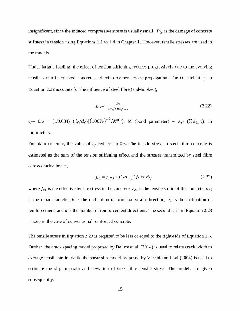
Under fatigue loading, the effect of tension stiffening reduces progressively due to the evolving

tensile strain in cracked concrete and reinforcement crack propagation. The coefficient 𝑐𝑓 in

Equation 2.22 accounts for the influence of steel fibre (end-hooked),

𝑓𝑐,𝑇𝑆= 𝑓𝑡𝑝

1+√3.6𝑐𝑓. 𝑐1 (2.22)

𝑐𝑓= 0.6 + (1/0.034) ( 𝑙𝑓/𝑑𝑓)[(100𝑉𝑓)1.5

/𝑀0.8]; M (bond parameter) = 𝐴𝑐/ (∑𝑑𝑏𝑠𝜋), in

millimeters.

For plain concrete, the value of 𝑐𝑓 reduces to 0.6. The tensile stress in steel fibre concrete is

estimated as the sum of the tension stiffening effect and the stresses transmitted by steel fibre

across cracks; hence,

𝑓𝑐1 = 𝑓𝑐,𝑇𝑆 + (1-𝛼𝑎𝑣𝑔)𝑓𝑓 𝑐𝑜𝑠𝜃𝑓 (2.23)

where 𝑓𝑐1 is the effective tensile stress in the concrete, 휀𝑐1 is the tensile strain of the concrete, 𝑑𝑏𝑖

is the rebar diameter, 𝜃 is the inclination of principal strain direction, 𝛼𝑖 is the inclination of

reinforcement, and n is the number of reinforcement directions. The second term in Equation 2.23

is zero in the case of conventional reinforced concrete.

The tensile stress in Equation 2.23 is required to be less or equal to the right-side of Equation 2.6.

Further, the crack spacing model proposed by Deluce et al. (2014) is used to relate crack width to

average tensile strain, while the shear slip model proposed by Vecchio and Lai (2004) is used to

estimate the slip prestrain and deviation of steel fibre tensile stress. The models are given

subsequently:

16

For steel fibre concrete,

𝑆𝑐𝑟 (average crack spacing) = 2(𝑐𝑎 + 𝑠𝑏

10) 𝑘3 +

𝑘1𝑘2

𝑠𝑚𝑖 (2.24)

where 𝑐𝑎 = 1.5𝑎𝑔𝑔; 𝑘1 = 0.4; 𝑘2 = 0.25; 𝑘3 = 1 – [min(𝑉𝑓, 0.015)/0.015][1-(1/𝑘𝑓)];

𝑎𝑔𝑔 is the maximum aggregate size, given in millimeters.

𝑠𝑏 = 1

√∑4

𝜋

𝜌𝑠,𝑖

𝑑𝑏,𝑖2 𝑐𝑜𝑠4𝜃𝑖𝑖

(2.25)

𝑠𝑚,𝑖 = ∑𝜌𝑠,𝑖

𝑑𝑏,𝑖 𝑐𝑜𝑠2𝜃𝑖𝑖 + 𝑘𝑓

𝛼𝑓𝑉𝑓

𝑑𝑓 (2.26)

For conventional reinforced concrete, 𝑆𝑐𝑟 = 1

|𝑐𝑜𝑠𝜃|/𝑠𝑚𝑥 +|𝑠𝑖𝑛𝜃|/𝑠𝑚𝑦

𝛿𝑠 (crack slip) = 𝛿2√𝜓

1−𝜓 (2.27)

𝛿2 = 0.5𝑣𝑐𝑚𝑎𝑥 +𝑣𝑐𝑜

1.8𝑤𝑐𝑟−0.8+(0.234𝑤𝑐𝑟

−0.707−0.20)𝑓𝑐𝑐 (2.28)

𝜓 = 𝑣𝑐𝑖,𝑐𝑟/𝑣𝑐𝑚𝑎𝑥; 𝑣𝑐𝑚𝑎𝑥 (in MPa) = √𝑓𝑐′/ [0.31 + (24𝑤𝑐𝑟

𝑎𝑔𝑔+ 16); 𝑣𝑐𝑜 = 𝑓𝑐𝑐/30; 𝑓𝑐𝑐 (in MPa), is taken

as the concrete cube strength; 𝑤𝑐𝑟 =𝑆𝑐𝑟휀𝑐1 . For conventional reinforced concrete, 𝛿𝑠 is taken as

𝛿2, but the numerator is replaced with the shear stress 𝑣𝑐𝑖 (Equation 2.27).

The shear strain resulting from the crack slip is estimated as 𝛾𝑠 = 𝛿𝑠/s; and resolving into x and y

components,

휀𝑥𝑠 = -𝛾𝑠/2. sin 2𝜃 (2.29)

휀𝑦𝑠 = 𝛾𝑠/2. sin 2𝜃 (2.30)

𝛾𝑥𝑦𝑠 = -𝛾𝑠/2. cos 2𝜃 (2.31)

Since the shear stresses and slip are functions of the reinforcement ratio or progressing principal

stresses, their values also evolve under fatigue loading. The tensile stress resulting from steel fibre

17

bridging deviates by an angle 𝜃𝑓 from the direction of the principal tensile stress (𝑓𝑐1). This

deviation angle, according to Lee et al. (2016), is estimated thus:

𝜃𝑓 = 𝑡𝑎𝑛−1 𝛿𝑠

𝑤𝑐𝑟 (2.32)

2.1.3.2 Conventional Reinforcement

Although a trilinear stress-strain relation is used to model the response of reinforcement in the

Disturbed Stress Field Model, a bilinear stress-strain relation (elastic-perfectly plastic) is used for

fatigue analysis. This is attributed to the fact that the behaviour of reinforcement under high cycle

fatigue loading is usually brittle; hence increased strength due to strain hardening is avoided.

18

CHAPTER 3: FINITE ELEMENT IMPLEMENTATION

3.1 Formulation

The general formulation of material stiffness matrix is expressed thus:

[𝜎] = [D] [휀] – [𝜎𝑜] (3.1)

{𝜎} and {휀} are the total stress and total strain vectors due to the applied maximum fatigue load.

(The ratio of the minimum to maximum fatigue loading is a parameter R required in a subsequent

section.) [𝐷] is the transformed composite stiffness matrix in which the concrete composite

degrades progressively due to fatigue loading.

{𝜎} = [

𝜎𝑥

𝜎𝑦

𝜏𝑥𝑦

] (normal and shear stresses on an element) (3.2)

{휀} = [

휀𝑥

휀𝑦

𝛾𝑥𝑦

] (corresponding strain values) (3.3)

[𝐷] = [𝐷𝑐 ] + ∑ [𝐷𝑠]𝑖𝑛𝑖=1 + [𝐷𝑓 ] (3.4)

Prior to cracking,

[𝐷𝑐] = 𝐸𝑐 (1−𝐷𝑡𝑒)

1−v2

[ 1

v

(1−𝐷𝑡𝑒) 0

v1

(1−𝐷𝑡𝑒)0

0 01−v

2(1−𝐷𝑡𝑒)]

(3.5)

As previously indicated, 𝐷𝑡𝑒 may be obtained using Equations 1.1 to 1.4 in Chapter 1. However,

∆𝑓 and 𝑓𝑐′ are replaced with the induced tensile stress and the concrete tensile strength of concrete,

respectively. For a given element strain condition, normal stresses in the concrete may be found

and subsequently, the principal tensile and compressive stresses and the principal strain direction

obtained.

19

For a two-dimensional cracked state, the stiffness of the concrete with respect to the axes of

orthotrophy, the stiffness of the steel reinforcement with respect to its direction, and the stiffness

of the steel fibre with respect to the inclination of tensile stress due to steel fibre are all required

(Equations 3.6 to 3.8). Subsequently, the stiffnesses are transformed back to the reference x, y axes

(Equations 3.9 and 3.10).

[𝐷𝑐]′ = [

𝐸𝑐1 0 0

0 𝐸𝑐2 0

0 0 𝐺𝑐

] for concrete (3.6)

𝐸𝑐1 = 𝑓𝑐1/휀𝑐1; 𝐸𝑐2

= 𝑓𝑐2/휀𝑐2; and 𝐺𝑐 =𝐸𝑐1

. 𝐸𝑐2 / (𝐸𝑐1

+ 𝐸𝑐2 )

[𝐷𝑠]𝑖′= [

𝜌𝑖𝐸𝑠𝑖 0 00 0 00 0 0

] for steel reinforcement (3.7)

𝐸𝑠𝑖 = 𝑓𝑠,𝑖/휀𝑠,𝑖

[𝐷𝑓]′ = [

𝜌𝑖𝐸𝑓1 0 0

0 0 00 0 0

] for steel fibre (3.8)

𝐸𝑓1 = 𝛼𝑎𝑣𝑔𝑓𝑓/휀𝑐𝑓; 휀𝑐𝑓 = (휀𝑐1 + 휀𝑐2)/2 + [(휀𝑐1- 휀𝑐2)/2]cos2𝜃𝑓

[𝐷𝑐 ] = [𝑇𝑐]𝑇[𝐷𝑐]

′[𝑇𝑐 ]; [𝐷𝑓 ] = [𝑇𝑓]𝑇[𝐷𝑓]

′[𝑇𝑓 ];

[𝐷𝑠,𝑖 ] = [𝑇𝑠,𝑖]𝑇[𝐷𝑠,𝑖]

′[𝑇𝑠,𝑖 ] (3.9)

[𝑇] = [

𝑐𝑜𝑠2𝜓 𝑠𝑖𝑛2𝜓 𝑐𝑜𝑠𝜓𝑠𝑖𝑛𝜓

𝑠𝑖𝑛2𝜓 𝑐𝑜𝑠2𝜓 −𝑐𝑜𝑠𝜓𝑠𝑖𝑛𝜓

−2𝑐𝑜𝑠𝜓𝑠𝑖𝑛𝜓 2𝑐𝑜𝑠𝜓𝑠𝑖𝑛𝜓 (𝑐𝑜𝑠2𝜓 − 𝑠𝑖𝑛2𝜓 )

](3.10)

For concrete, 𝜓 = 𝜃𝑐, for steel fibre, 𝜓 = 𝜃𝑐 + 𝜃𝑓, and for a steel reinforcing bar, 𝜓 = 𝛼𝑖.

𝜎𝑜 (Equation 3.11) is estimated as a pseudo-load using Equations 2.8 to 2.16 in Chapter 2. For a

given stress condition and loading cycle (due to applied fatigue load), the total strain in the element

20

can be obtained. The solution approach is iterative since the secant moduli of materials are needed

to find the strain condition {휀} and vice versa.

[𝜎𝑜] = [𝐷𝑐 ] ([휀𝑐𝑝] + [휀𝑐

𝑜] + [휀𝑐𝑠] + [휀𝑐

𝑓𝑎𝑡]) (3.11)

In the iterative process for an element at the first fatigue loading cycle, strain values are initially

assumed. Subsequently, the principal strain values and the corresponding inclination of the

principal tensile strain are estimated. Using the modified compatibility and constitutive equations

illustrated previously, the net strains are estimated and subsequently, the average principal stresses

in the concrete and the average stresses in the reinforcement are obtained with the assumption that

fatigue damage is zero.

Stresses at the crack are also checked and shear stress and crack slip are estimated using the

modified equilibrium equation; however, Zo is assumed to be zero for the first cycle. From the

crack slip, prestrains are estimated and are subtracted from the total strains in order to obtain net

strains. Further, secant moduli for the constituent materials are estimated and the material stiffness

matrices are obtained using Equations 3.7 to 3.10. Subsequently, the total strains are obtained and

compared with the previous values assumed (Equation 3.12). The iterative process continues until

the errors become minimal. The element stresses estimated are saved for subsequent loading

cycles.

[휀] = [D]-1 ([𝜎] + [𝜎𝑜]) (3.12)

For subsequent fatigue loading cycles, the saved stresses and the number of fatigue loading cycles

considered are substituted into the corresponding fatigue damage model (described in Chapter 1)

to estimate the required damage for the irreversible strain, the modified constitutive models, and

the modified equilibrium equations. The described iterative process is also repeated as the fatigue

21

loading cycles are increased. Failure becomes imminent when instability due to fractured

reinforcement or significant crushing of concrete occurs. Deformation evolution plots can be

obtained from the material parameter values as the fatigue loading cycles are increased up to the

point of failure.

Fig. 3.1 - Flow chart for the modified solution algorithm for DSFM.

Total Nodal Force Vector

Element Stiffness Matrices

Global Stiffness Matrices

Global Joint Displacements

Check Convergence

Update Stress/Strain Parameters

Total Element Strains

Fatigue damage model for

𝑓𝑐′ and 𝑓𝑡

𝐷𝑓𝑐 (𝑁, 𝑓𝑐2), 𝐷𝑓𝑡(𝑁, 𝑓

𝑐1)

𝐷𝑓𝑒 (𝑁, 𝑓𝑐2), 𝐷𝑡𝑒(𝑁, 𝑓

𝑐1)

CONCRETE DAMAGE

MODEL

ai (N)

aj (N, 𝑓𝑠𝑖 )

FRACTURE MECHANICS

Determine element component strains [𝜖𝑠

𝑜]𝑖 ,[𝜖𝑐𝑠], [𝜖𝑐

𝑜], [𝜖𝑐𝑝]

Determine concrete/reinforcement stresses 𝑓𝑐1, 𝑓𝑐2, 𝑓𝑠𝑖

Determine local stresses at cracks 𝒇𝒔𝒄𝒓𝒊 , 𝒗𝒄𝒊

Determine crack slip strains and fatigue strain

𝜹𝒔 , 𝜸𝒔 , [𝝐𝒔], [𝜺𝒄𝒇𝒂𝒕

]

Determine material

secant moduli

��𝒄𝟏 , ��𝒄𝟐 , ��𝒄 , ��𝒔𝒊

Determine material stiffness matrices [𝑫𝒄] , [𝑫𝒔]𝒊 , [𝑫]

Determine element

prestress vector [𝜎𝑜]

Determine new

estimates of strain

[𝜖] , [𝜖𝑐]

Irreversible compressive

fatigue strain

A

B

C

1

2

Per Finite Element

3

4

5

6

7

8

MODIFIED CONSTITUTIVE MODEL

휀𝑑(𝐷𝑓𝑐, 𝐷𝑓𝑒 𝑁, 𝑓𝑐2, 휀𝑐2)

LS =1

LS >1

LS =1

LS >1

LS =1

LS >1

LS: Load stage

22

The modified algorithm for the Disturbed Stress Field Model which accounts for fatigue damage

in an element is shown in the flow chart in Figure 3.1. The original algorithm is void of the damage

models (A, B, and C). In all, the analyses involve modelling the monotonic loading responses of

structural components which exhibit some level of damage due to fatigue loading cycles.

3.2 Failure Criterion for Reinforced Concrete and Steel-Fibre Concrete under Fatigue

Loading

The evolution of deformation is attributed to plain or steel fibre concrete strength and stiffness

deterioration, irreversible strain accumulation, and steel reinforcement crack growth (A, B, and C

in Figure 3.1). Monotonic tests of structural elements subjected to different fatigue loading cycles

will exhibit decreasing resistance capacity as the loading cycles increase. The number of cycles at

which the residual capacity of the element becomes equal to the fatigue load is termed the fatigue

life of the structural element. At this instant, severe crushing of concrete or fracture of reinforcing

bars may occur, leading to structural collapse.

For further exemplification, the solution to the fatigue analysis of a shear panel is illustrated using

the flow chart given in Figure 3.1 in a stepwise manner. The properties and loading parameters are

also given. Three different pure shear fatigue loads (Figure 3.2) (3.5 MPa, 3.0 MPa, and 2.7 MPa)

were used and the corresponding deformation evolution of the material parameters were obtained.

The significance of the proposed analysis approach can be observed from the predicted three-

staged deformation evolution plots. In addition, the effect of fatigue loading is explicitly shown in

all plots given in Figures 3.3 to 3.8.

23

Fig. 3.2 - Shear panel (PV19).

𝑓𝑐′ = 19.0 MPa; 𝜌𝑥 = 1.785%

𝑓𝑡′ = 1.72 MPa; 𝜌𝑦 = 0.713%

휀𝑐′ = -2.15 x 10−3; 𝑓𝑦𝑥 = 458 MPa

𝑓𝑦𝑦 = 300 MPa

𝐸𝑠 = 200000 MPa

𝑎 = 10 mm

𝑠𝑥 ≈ 50 mm 𝑑𝑏𝑥 ≈ 6.35 mm

𝑠𝑦 ≈ 50 mm 𝑑𝑏𝑦 ≈ 4.01 mm

Fatigue frequency = 5 Hz waveform = sinusoidal

Load ratio (R) = 0

[𝜎] = [00

3.0] MPa

Solution:

The assumed initial total and net strains (from previous calculations) for an applied shear stress of

3.0 MPa on the shear element in Figure 3.2, are:

{휀} = [0.4310.7921.725

] x 10−3 {휀𝑐} = [0.5660.6591.716

] x 10−3

𝝉𝒙𝒚 = 3 MPa

Y

X

𝝉𝒙𝒚

24

Using the iterative process described previously, the monotonic response of the shear panel which

includes induced stress and strain values due to the applied fatigue load (3.0 MPa) is obtained

(without considering fatigue damage). The obtained and saved element stresses due to the

monotonic response or at the first cycle, required in calculating damage values in subsequent

cycles, are given thus:

fsx = 111 MPa; fsy = 241 MPa (both stresses are required in the fracture mechanics model)

fc2 = -5.35 MPa; fc1 = 1.08 MPa (required in concrete damage model and irreversible strain model).

These values are substituted into A, B, and C in Figure 3.1 to estimate the corresponding damage

at any given fatigue loading cycle. Having accounted for the corresponding damage, the monotonic

response is again obtained iteratively. This is repeated for given cycles until instability is reached.

3.3 Solution for Fatigue Loading at 10000 cycles

Figure 3.1 (Box 1) - Strain components after iterations are:

{휀} = [0.5841.2782.604

] x 10−3 {휀𝑐} = [0.8041.0722.569

] x 10−3

The principal strains are estimated from {휀𝑐} (Equations 2.15 and 2.16 in Chapter 2) as:

휀𝑐1 = 2.23 x 10-3 휀𝑐2 = -0.353 x 10-3 𝜃𝜎= 42.020

Figure 3.1 (Box 2) - Average Stresses in Concrete and Reinforcement:

Since the concrete is in a cracked state, Equations 1.18 to 1.19 in Chapter 1 are used for concrete

compressive stress. The damage parameter required in the equation is obtained from Equations 1.1

to 1.3. The fatigue prestrain value (Equation 2.12 to 2.14) is also required in estimating the concrete

compressive stress.

fc2 = 5.34 MPa

fc1 = 1.07 MPa

25

Assuming perfect bond between the concrete and the steel reinforcement, the average strain in the

concrete is equal to the average strain in the steel reinforcing bars. Hence:

𝐸𝑠 = 200000 MPa

휀𝑠𝑥 = 0.584 x 10−3

휀𝑠𝑦 = 1.278 x 10−3

𝑓𝑠𝑥 = 𝐸𝑠 휀𝑠𝑥 = 117 MPa (x-direction)

𝑓𝑠𝑦 = 𝐸𝑠 휀𝑠𝑦 = 256 MPa (Y-direction)

Figure 3.1 (Box 3) - Local stresses at crack:

The local stresses are estimated from Equations 2.6 and 2.7 (neglecting the influence of steel fibre).

In Equations 2.6 and 2.7, the reinforcement crack growth factor (Zo) is estimated from Equations

1.10 to 1.16 (shown as C in Figure 3.1). The average reinforcement stresses are required in C in

order to estimate the progressive crack depth; Thus:

휀𝑠𝑐𝑟𝑥 = 1.033 x 10-3 , 𝑓𝑠𝑐𝑟𝑥 = 207 MPa

휀𝑠𝑐𝑟𝑦 = 1.642 x 10-3 , 𝑓𝑠𝑐𝑟𝑦 = 300 MPa

vci = 0.621 MPa

Figure 3.1 (Box 4) - Crack slip strains:

The slip at a given fatigue loading cycle can be estimated using Equation 2.27. Subsequently, the

shear strains (in x-y directions) resulting from slip at the crack are estimated. Fatigue irreversible

compressive strain values are also estimated in the x-y direction (Equations 2.12 to 2.14). The

prestrain is equal to the summation of the shear strains. The pseudo-load [𝜎𝑜] is estimated from

the obtained values of prestrain.

The shear strain resulting from the crack slip is estimated as: 𝛾𝑠 = 𝛿𝑠/s = 0.429 x 10-3; resolving

into x and y components,

26

휀𝑥𝑠 = -𝛾𝑠/2. sin 2𝜃 = -0.213 x 10-3

휀𝑦𝑠 = 𝛾𝑠/2. sin 2𝜃 = 0.213 x 10-3

𝛾𝑥𝑦𝑠 = -𝛾𝑠/2. cos 2𝜃 = 0.022 x 10-3

Inclusion of the irreversible fatigue strain is done in the manner of an offset strain:

휀𝑥𝑓𝑎𝑡

= 휀𝑐,2𝑓𝑎𝑡

/2 . (1- cos 2𝜃)= -6.09 x 10-6

휀𝑦𝑓𝑎𝑡

= 휀𝑐,2𝑓𝑎𝑡

/2 . (1+ cos 2𝜃) = -7.50 x 10-6

𝛾𝑥𝑦𝑓𝑎𝑡

= - 휀𝑐,2𝑓𝑎𝑡

/2 . sin 2𝜃 = 13.5 x 10-6

Figure 3.1 (Box 5) - Material secant moduli:

The net strain values are estimated from Equation 2.8 (for concrete). The ratio of the average stress

to the net strain gives the secant modulus for concrete. In the case of steel reinforcement, the ratio

of the average stress in steel reinforcement to the induced strain gives the secant modulus.

Ec1 = 480 MPa

Ec2 = 15124 MPa

Gc = 466 MPa

Esx = 200000 MPa

Esy = 200000 MPa

Figure 3.1 (Box 6) - Material stiffness matrices [Dc], [Ds], [D]:

The stiffness matrices are estimated from Equations 3.4 to 3.8. The transformed composite

stiffness matrix is obtained using Equation 3.9. The transformed composite stiffness matrix at

10000 cycles was obtained thus:

[D] = [7213 3367 −32563367 6653 −3992

−3256 −3992 3861] (MPa)

Figure 3.1 (Box 7) - Determine element prestress vector [𝜎𝑜]:

27

The element prestress vector was estimated from Equation 3.11. Herein, two prestrain values were

considered: the shear strain at crack and the fatigue irreversible strain. The summation of the

prestrains is equal to: [휀𝑝𝑠0 ] = [

−0.220.213.58

] x 10-3 and,

[𝜎𝑜] = [−0.130.26

−5.35] MPa

Figure 3.1 (Box 8) - Determine new estimates of strain {휀}, {휀𝑐}:

The total and net strain values are estimated using Equation 3.12. Since the results presented herein

were obtained after convergence, the final values were also equal to the initial values. However,

where significant variations are observed, the iteration continues as illustrated using the given

steps. This procedure was repeated as the number of fatigue loading cycles was increased.

At the final collapse or failure of a structural element (in this case, the shear reinforcement in the

vertical direction failed first), instability is observed and significant deformation persists. The

results for the three different loads used are given in Figures 3.3 to 3.8. They are presented in terms

of the crack slip evolution, shear stress evolution, reinforcement crack depth propagation (in the

Y-direction where failure occurred), reinforcement strain, and stress evolutions.

The influence of fatigue load on the fatigue life is well-captured as observed in all deformation

evolution plots (Figures 3.3 to 3.8). As the fatigue load increased, the corresponding fatigue life

reduced, and the rates of deformation were observed to increase. In addition, the significance of

the proposed approach stems from the fact that the profiles obtained in each case resemble the

well-known fatigue deformation profile for reinforced concrete. Based on these observations, the

deformation evolution within the cracked plane in reinforced concrete or steel fibre concrete can

be obtained using the proposed approach.

28

Fig. 3.3 - Crack slip evolution.

Fig. 3.4 - Shear stress evolution at crack.

Fig. 3.5 - Reinforcement (Y-direction) crack growth depth.

29

Fig. 3.6 - Reinforcement (X-direction) strain evolution at crack location.

Fig. 3.7 - Reinforcement (X-direction) average stress evolution.

Fig. 3.8 - Localised reinforcement strain evolution (Y–direction).

30

CHAPTER 4: USE OF VecTor2 FOR FATIGUE DAMAGE ANALYSIS

VecTor2 nonlinear finite element analysis software was modified to account for fatigue damage

analysis using the concepts described in the preceding Chapters. The approach for modelling of a

structural element using Formworks is well documented in VecTor2 user’s manual; however, this

is reiterated alongside the new features for incorporating fatigue damage analysis.

Figure 4.1- Formwork application window.

4.1 Defining Concrete Materials

The icon above (pointed in step 1) is selected to input the material and geometrical properties for

concrete such as thickness, compressive and tensile strengths, aggregate size, average crack

spacing, etc. (Figure 4.2). For smeared reinforced concrete, the reinforcement component

properties can also be included; however, the reference type box is used. For fatigue analysis,

asides from steel fibre concrete, conventional reinforced concrete structural elements should be

modelled using discrete reinforcement and the corresponding bond properties. For steel fibre-

Step 1: Material

properties

Step 2: Reinforcement properties

Step 3: Bond

properties

Step 4: Mesh

structure

Step 6: Job

definition Step 5: load application

31

reinforced concrete, other parameters for flexural strength (Model Code 2010) may be

implemented within the smeared reinforcement properties.

Figure 4.2 – Reinforced concrete materials properties dialog box.

4.2 Defining Reinforcement Properties

For high-cycle fatigue life prediction, fracture of reinforcing steel or structural collapse is assumed

to be brittle. As such, yielding of steel reinforcement coincides with fatigue failure. The

reinforcement properties (Figure 4.3) in the Define Reinforcement Materials dialog box are

selected such that the strain-hardening of steel reinforcement is neglected. The ultimate yield

strength of the selected ductile steel reinforcement should have the same value as the yield strength

(variation of about 1% at most). Other corresponding properties such as cross-section area,

reinforcement diameter, elastic modulus etc. are also required.

32

Fig. 4.3 – Reinforcement materials dialog box.

4.3 Bond Types

As described in VecTor2 user’s manual for bond stress-slip relationships between concrete and

discrete reinforcement under different loading conditions, the reference type of steel bars, the bond

properties, bar clear cover, number of reinforcement layers for embedded bars, etc. are selected

(mainly embedded deformed bars) as shown in Figure 4.4.

Figure 4.4 – Bond properties dialogue box.

33

4.4 Structure and Mesh Definition

The creation of the element or concrete regions, inclusion of discrete steel reinforcement, inclusion

of attributes such as bond type, discretization and mesh type, indication of constraints, and

meshing, are well illustrated in VecTor2 user’s manual. This is indicated as step 4 in Figure 4.1.

Figure 4.5 – structure and mesh definition.

4.5 Load Application under Fatigue Loading

A fatigue waveform is shown in Figure 4.6, with the indication of the maximum and the minimum

fatigue loads. Basically, the maximum fatigue load is required for loading in VecTor2. However,

34

the effect of the minimum fatigue loading in high-cycle fatigue is accounted for using the load

ratio R (𝐹𝑚𝑖𝑛

𝐹𝑚𝑎𝑥

). (Note: this is indicated as step 5 in Figure 4.1).

Fig. 4.6 – Fatigue load wave form (sinusoidal)

Figure 4.7 – Load application

The direction of the maximum load is considered by indicating a negative sign for a vertical force

acting downwards. In addition, a unit load is indicated at the corresponding node where the fatigue

load acts. The concept of load factor will be discussed subsequently.

4.6 Job Definition

The implementation of fatigue parameters is considered within the Define job dialog box. The

procedure for appropriate model selection is illustrated thus

In the Define job dialog box (Figure 4.8), the first box corresponds to the job control. Herein, the

maximum fatigue load is entered as the initial factor, while a reasonable increment (usually 0.5

Maximum fatigue load

(𝐹𝑚𝑎𝑥)

Minimum fatigue load (𝐹𝑚𝑖𝑛)

35

or 1.0) is also typed in the box for the incremental factor. All other parameters may be selected

as described in VecTor2 user’s manual.

Figure 4.8 – Job control.

The models to be used are obtained by clicking on the Models button in the Define job dialog box.

Under fatigue loading for concrete material, the Hognestad’s equation or Popovics’ equation for

compression can be used depending on the type of concrete (normal or high strength, respectively).

For the normal strength-compression post-peak, the modified Park-Kent is used, while the

Popovics/Mander model is used for the high strength concrete compression post-peak. Asides the

compression pre-peak and Post-peak models, other models required are similar for normal and

high strength concrete (default values are recommended). These are shown in Figure 4.9 for high-

strength plain concrete.

Maximum

fatigue load

Incremental

factor

36

In the case of steel fibre-reinforced concrete, Lee et al. (2011) FRC models are used. For

compression softening, the Vecchio 1992-A (e1/e2) model is recommended, while the Advanced

Lee (2009) model is suggested for crack stress calculation. Further, Vecchio and Lai’s model is

recommended for the crack slip calculation, the Lee 2010 (w/post-yield) model is suggested for

tension stiffening, and the FIB model code 2010 is used for tension softening. The reinforcement

models are left as default.

Fig. 4.9 – Concrete models

4.7 Defining Fatigue Loading Parameters in Job

In the Job dialog box, select special.

Select Considered within the tray corresponding to Concrete/Reinf. Fatigue (Figure 4.10).

Click on Show Fatigue Parameters (Figure 4.11). The boxes are filled appropriately with values

for frequency (in Hertz), loading ratio (R), fatigue wave-form, permissible error (0.01 default),

37

and interval of loading cycles. The number of fatigue loading cycles is increased for each analysis

conducted. Basically, the load-deformation plot is obtained for different loading cycles. As the

number of cycles included increases, the load capacity reduces and the deformation increases. An

instance is reached when the load capacity is approximately equal to the fatigue load (used as the

initial factor in Figure 4.8). The corresponding number of cycles is the fatigue life.

4.10 – Fatigue damage consideration

38

Fig. 4.11 – Fatigue damage parameters

For reduced analysis time, a reasonable interval should be chosen for the fatigue analysis. For

example, the ratio of the selected number of cycles to the interval of loading cycles may be taken

as 100 or 1000.

4.8 Solved example

Fig. 4.12 - Details of deep beam specimen.

The solution to the fatigue life prediction of the beam given in Figure 4.12 using Formworks

modelling procedure/VecTor2 analysis is presented. Herein, the fatigue life of the beam when

subjected to a fatigue load of 80% of the ultimate load is considered (Figure 4.13). From an initial

monotonic load-deformation response without fatigue damage, an ultimate load capacity value of

245 kN was obtained from the model (Figure 4.14); hence, 80% of the capacity is equal to 196 kN.

30

30

2 LEGS (D4)

2-10M/2-15M

175

250

X

X

700

100

250

124

30

30

128

64

426

Beam with 0.2% shear reinforcement ratio Section X-X

D4- fY = 610MPa

10M- fy = 480 MPa

𝑓𝑐′ = 59 MPa

휀𝑐′ = 0.002

𝑓𝑡′ = 2.3 MPa

39

This value corresponds to the maximum fatigue load to be used. The loading frequency was

assumed to be 5 Hz, while the fatigue loading ratio and fatigue waveform were assumed to be zero

and 0.15 (sinusoidal wave), respectively. The residual capacities which correspond to different

fatigue loading cycles are shown in Figure 4.15. As observed, at 40 000 cycles, the loading cycles

was approximately close to the applied fatigue load; hence, its failure instance. The mid-span

deflection evolution is also given in Figure 4.16. Towards failure, the rate of increase was higher.

Other results such as reinforcement stresses or strains as the loading cycles increase can also be

obtained. As indicated initially, structural failure due to high-cycle fatigue loading will occur when

the reinforcing bars fracture (Figure 4.17). This corresponds to the yield value of the

reinforcement. As shown in Figure 4.17, the shear reinforcement did not fracture; rather, collapse

was a result of the longitudinal reinforcement stress reaching the yield value (max stress in

reinforcement at 40 000 cycles corresponds to the yield value of 480 MPa – Figure 4.12).

Fig. 4.13 – Finite element mesh for beam.

40

Fig. 4.14 – Load versus mid-span deflection.

Fig. 4.15 – Fatigue residual capacity.

0

100

200

300

0 10 20

Lo

ad (

kN

)

Mid-span deflection (mm)

196

200

204

208

212

0.54 0.79 1.04 1.29

Load

(kN

)

Mid-span deflection (mm)

500 cycles

1500 cycles

5000 cycles

10000 cycles

20000 cycles

30000 cycles

40000 cycles

41

Fig. 4.16 – Mid-span deflection evolution.

Fig. 4.17 – Evolution of stresses in reinforcing bars (stresses shown in MPa).

0.5

0.9

1.3

0 10 20 30 40 50

Mid

-span

def

lect

ion

(mm

)Number of cycles ( x 103)

500 cycles

40000 cycles

42

5.0 SUMMARY AND RECOMMENDATION

5.1 Summary

An approach which can be used to predict the fatigue life of a reinforced concrete structural

element using VecTor2 was illustrated. The analysis was based on the implementation of fatigue

damage mechanisms in concrete and steel reinforcement, especially at the cracked concrete plane.

The founding principle (for appropriately reinforced concrete elements) assumes that the fatigue

life corresponds to the instance at which the fatigue residual capacity becomes equal to the fatigue

load applied. This has been shown to be realistic based on validation of experimental investigations

with finite element analysis using the proposed approach.

5.2 Recommendation

Depending on the complexity of the structural element and the density of embedded reinforcement,

certain anomalies may occur while modelling. For ease, reasonable interval of fatigue loading

cycles and load increments should be used at intervals especially at instances when the degradation

becomes significant. The use of an elastic-perfectly plastic model for steel reinforcement is

reiterated and strongly encouraged, as this dictates the fatigue residual capacity. Since high-cycle

fatigue is brittle in nature, the increased strain values in steel reinforcement due to crack growth

should not take into account the strain hardening effects. This obviously accounts for the

substantial increase in reinforcement temperature as cracks propagate.

43

6.0 REFERENCES

Amir et al. (2012). “Fatigue Performance of High-Strength Reinforcing Steel.” Journal of Bridge

Engineering, Vol. 17, No. 3, pp. 454-461.

British Standard (2005). “Guide to Methods for Assessing the Acceptability of Flaws in Metallic

Structures.” BS 7910.

Collins, M.P., Mitchell, D. (1997). “Prestressed Concrete Structures.” Response Publications,

Canada, 766 pp.

Cook D.J., and Chindaprasirt P. (1980). “Influence of Loading History upon the Compressive

Properties of Concrete.” Magazine of Concrete Research, Vol. 32, No. 111, 1980, pp. 89-100.

Deluce, J.R., Lee, S.C, and Vecchio, F. (2014). “Crack Model for Steel Fibre-Reinforced

Concrete Members Containing Conventional Reinfocement.” ACI Structural Journal, Vol. 111,

No. 1, pp. 93-102.

Dowling, N.E. 1993. Mechanical Behaviour of Materials, Prentice Hall, New Jersey.

Edalatmanesh R., and Newhook J.P. (2013). “Residual Strength of Precast Steel-Free Panels.”

ACI Structural Journal, Vol.110, pp. 715-722.

Isojeh, B., El-Zeghayar, M., and Vecchio, F.J. (2017a). “ Concrete Damage under Fatigue

Loading in Uniaxial Compression.” ACI Materials Journal, Vol. 114, No. 2, pp. 225-235.

Isojeh, B., El-Zeghayar, M., and Vecchio, F.J. (2017b). “ Simplified Constitutive Model for

Fatigue Behaviour of Concrete in Compression.” Journal of Materials in Civil Engineering, DOI:

10.1061/(ASCE)MT.1943-5533.0001863.

44

Gao L., and Hsu C.T.T. (1998). “Fatigue of Concrete under Uniaxial Compression Cyclic

Loading.” ACI Materials Journal, Vol. 95, No. 5, pp. 575-581.

Herwig A. (2008). “Reinforced Concrete Bridges under Increased Railway Traffic Loads-

Fatigue Behaviour and Safety Measures.” Ph. D Thesis No. 4010, Ecole Polytechnique Federale

de Lausanne.

Hirt, M.A., Nussbaumer, A. 2006. Construction metallique: notions fondamentales et methods de

dimensionnement, nouvelle edition revue et adaptee aux nouvelles norms de structures. Traite de

Genie Civil de l’Ecole Polytechnique Federale, Vol. 10. Lausanne, Switzerland.

Holmen J.O. (1982). “Fatigue of Concrete by Constant and Variable Amplitude Loading.”

ACI SP Vol. 75, No. 4, pp. 71-110.

Isojeh, B., El-Zeghayar, M., and Vecchio, F.J. (2017c). “ Fatigue Behaviour of Steel Fibre

Concrete in Direct Tension.” Journal of Materials in Civil Engineering, DOI:

10.1061/(ASCE)MT.1943-5533.0001949.

Isojeh B., El-Zeghayar M., Vecchio, F.J. “Fatigue Resistance of Steel-Fibre Reinforced Concrete

Deep Beams.” ACI Structural Journal, Vol. 114, No. 5, pp. 1215-1226.

Isojeh B., El-Zeghayar M., Vecchio, F.J. (2017e). “High-Cycle Fatigue Life Prediction of

Reinforced Concrete Deep Beams.” Engineering Structures Journal, Vol. 150, pp. 12-24.

Isojeh, M.B., and Vecchio, F.J (2016). “Parametric Damage of Concrete under High-Cycle Fatigue

Loading in Compression.” Proc., 9th International Conference on Fracture mechanics of Concrete

and Concrete Structures. FraMCoS-9 2016; 10.21012/FC9.009.

45

Lee, S.C., Cho, J.Y., Vecchio, F.J. (2016). “Analysis of Steel Fibre-Reinforced Concrete Elements

Subjected to Shear.” ACI Structural Jorunal, Vol. 113, No. 2, pp. 275-285.

Paris, P., Gomez, M.P., and Anderson W.E. (1961). “A Rational Analytical Theory of Fatigue.”

The Trend in Engineering, Vol. 13, pp. 9-14.

Rocha M., and Bruhwiler E. (2012). “Prediction of Fatigue Life of Reinforced Concrete Bridges.”

In Biondini and Frangopol (Eds) Bridge Maintenance, Safety, Management, Resilience and

Sustainability, pp. 3755-3760.

Schaff J.R., and Davidson B.D. (1997). “Life Prediction Methodology for Composite Structures.

Part 1- Constant Amplitude and Two-Stress Level Fatigue.” Journal of Composite Materials, Vol.

31, No. 2, pp. 128-157.

Vecchio F.J. (2000). “Disturbed Stress Field Model for Reinforced Concrete: Formulation.”

Journal of Structural Engineering, Vol. 127, No. 1, pp. 1070-1077

Vecchio F.J. (2001). “Disturbed Stress Field Model for Reinforced Concrete: Implementation.”

Journal of Structural Engineering, Vol. 127, No. 1, pp. 12- 20.

Vecchio, F.J., Lai, D., Shim, W., Ng, J. (2001). “Disturbed Stress Field Model for Reinforced

Concrete: Validation.” Journal of Structural Engineering, Vol. 127, No. 4, pp. 350-358.

Zhang B., Phillips D.V., and Wu K. (1996). “Effects of Loading Frequency and Stress Reversal

on Fatigue Life of Plain Concrete.” Magazine of Concrete Research, Vol. 48, pp. 361-375.