Low-Order Modeling, Controller Design
and Optimization of Floating Oshore Wind
Turbines
A thesis accepted by the Faculty of Aerospace Engineering and Geodesy of the
University of Stuttgart in partial fulllment of the requirements for the degree of
Doctor of Engineering Sciences (Dr.-Ing.)
by
Frank Lemmer (né Sandner)
born in Ostldern-Ruit, Germany
Main referee: Prof. Dr. Po Wen Cheng
Co-referee: Prof. Dr. Carlo L. Bottasso
Date of defense: 2.07.2018
Institute of Aircraft Design
University of Stuttgart
2018

Cover images courtesy of Henrik Bredmose, showing Research Laboratory in Hydrodynamics, Energetics &
Atmospheric Environment, Nantes, France (large) and Danish Hydraulic Institute (DHI), Hørsholm, Denmark
(small).

Acknowledgements
I would like to sincerely thank everybody who contributed in one way or the other to the
completion of this thesis. First, a special thanks to my family, particularly my wife and my
fabulous kids, who gave me the strength and the freedom to pursue this endeavor all the way
through its highs and lows to the nish line.
It has been a true pleasure to work all the years at SWE with a dedicated and motivated
team, where everyone is used to taking on responsibility with a continuous sense of collegiality
and support for each other. Prof. Dr. Po Wen Cheng is the one who enables everyone to pursue
their goals and a person who helped me to always keep the big picture in mind. I had the
pleasure to work with Prof. Dr. David Schlipf, who introduced me to the eld of wind energy
and always found a way to motivate me to face the next challenge through his unagging
commitment to research. Working closely with Dr. Denis Matha kick-started me in the eld
of oating oshore wind. I have enjoyed working with the oating wind fellows Friedemann
Borisade and Kolja Müller, who were always there for discussions. Wei (Viola) Yu completed
two study projects under my supervision and I am more than happy that she decided to also
pursue a Ph.D. She keeps asking the right questions and pushes the limits of oating wind
control forward. I enjoyed the discussions on controls with Dr. Steen Raach and the exchange
on aerodynamics and multibody dynamics with Birger Luhmann.
For technical advice throughout this thesis, I would like to express my sincere gratitude to
Dr. Jason Jonkman of NREL, who, with his attentive support on the open-source FAST pro-
gram, has contributed to the ndings of this thesis. The same holds for Prof. Dr. Henrik
Bredmose of DTU and Dr. Amy Robertson of NREL, who were always encouraging and
ready for lively discussions on oshore hydrodynamics. In the project INNWIND.EU, which
funded parts of this thesis, I always appreciated the pleasant cooperation with Dr. José Azcona
of CENER and Dr. Filippo Campagnolo of TUM. In LIFES50+, which funded the second half
of this work, I enjoyed a very constructive collaboration with Dr. Antonio Pegalajar-Jurado and
Dr. Michael Borg. I am also indebted to the project AFOSP, which initiated the rst successful
oater design studies together with Prof. Dr. Climent Molins and Alexis Campos of UPC.
Numerous Bachelor's and Master's students contributed to my research at SWE. I would
like to thank Florian Amann for his invaluable support with the building of scaled models. My
gratitude also goes to Christian Koch, Barbara Mayer, Daniel Walia, Junaid Ullah, Arne Härer,
Guillermo Abón, Fabian Brecht and all others.


Contents
Abbreviations ix
Symbols xiii
Abstract xix
Kurzfassung xxi
1 Introduction 1
1.1 Motivation . . . . . . . . . . . . . . . . . . . . . . . . . . . . . . . . . . . . . . . 11.2 Related Work . . . . . . . . . . . . . . . . . . . . . . . . . . . . . . . . . . . . . 31.3 Aim and Scope . . . . . . . . . . . . . . . . . . . . . . . . . . . . . . . . . . . . 41.4 Notation . . . . . . . . . . . . . . . . . . . . . . . . . . . . . . . . . . . . . . . . 5
2 Background 7
2.1 Oshore Wind Energy . . . . . . . . . . . . . . . . . . . . . . . . . . . . . . . . 72.2 Floating Oshore Wind Energy . . . . . . . . . . . . . . . . . . . . . . . . . . . 82.3 Comparison of Platform Types . . . . . . . . . . . . . . . . . . . . . . . . . . . 82.4 Optimization and Systems Engineering . . . . . . . . . . . . . . . . . . . . . . . 102.5 Dynamics of Floating Wind Turbines . . . . . . . . . . . . . . . . . . . . . . . . 11
2.5.1 Structural dynamics . . . . . . . . . . . . . . . . . . . . . . . . . . . . . 152.5.2 Aerodynamics . . . . . . . . . . . . . . . . . . . . . . . . . . . . . . . . . 162.5.3 Hydrodynamics . . . . . . . . . . . . . . . . . . . . . . . . . . . . . . . . 192.5.4 Mooring dynamics . . . . . . . . . . . . . . . . . . . . . . . . . . . . . . 28
2.6 Linear Frequency-Domain Modeling . . . . . . . . . . . . . . . . . . . . . . . . . 292.7 Environmental Conditions and Load Calculation . . . . . . . . . . . . . . . . . . 31
2.7.1 Wind . . . . . . . . . . . . . . . . . . . . . . . . . . . . . . . . . . . . . . 312.7.2 Waves . . . . . . . . . . . . . . . . . . . . . . . . . . . . . . . . . . . . . 322.7.3 Design loads . . . . . . . . . . . . . . . . . . . . . . . . . . . . . . . . . . 32
2.8 Model Tests . . . . . . . . . . . . . . . . . . . . . . . . . . . . . . . . . . . . . . 372.9 Control . . . . . . . . . . . . . . . . . . . . . . . . . . . . . . . . . . . . . . . . 39
2.9.1 Variable speed blade-pitch-to-feather-controlled turbines . . . . . . . . . 392.9.2 Floating wind turbines . . . . . . . . . . . . . . . . . . . . . . . . . . . . 40
2.10 Reference Design . . . . . . . . . . . . . . . . . . . . . . . . . . . . . . . . . . . 43
3 Development of a Low-Order Simulation Model 45
3.1 Requirements . . . . . . . . . . . . . . . . . . . . . . . . . . . . . . . . . . . . . 453.2 Structural Model . . . . . . . . . . . . . . . . . . . . . . . . . . . . . . . . . . . 46
3.2.1 Rigid multibody systems . . . . . . . . . . . . . . . . . . . . . . . . . . . 473.2.2 Flexible multibody systems . . . . . . . . . . . . . . . . . . . . . . . . . 523.2.3 Additional dynamic couplings . . . . . . . . . . . . . . . . . . . . . . . . 61

vi Contents
3.2.4 Symbolic programming . . . . . . . . . . . . . . . . . . . . . . . . . . . . 613.2.5 Linearization . . . . . . . . . . . . . . . . . . . . . . . . . . . . . . . . . 613.2.6 Time-domain motion and load response signals . . . . . . . . . . . . . . 623.2.7 Frequency-domain motion and load response spectra . . . . . . . . . . . 63
3.3 Wind Model . . . . . . . . . . . . . . . . . . . . . . . . . . . . . . . . . . . . . . 653.4 Aerodynamic Model . . . . . . . . . . . . . . . . . . . . . . . . . . . . . . . . . 66
3.4.1 Nonlinear model . . . . . . . . . . . . . . . . . . . . . . . . . . . . . . . 663.4.2 Linearized model . . . . . . . . . . . . . . . . . . . . . . . . . . . . . . . 67
3.5 Hydrodynamic Model . . . . . . . . . . . . . . . . . . . . . . . . . . . . . . . . . 683.5.1 Radiation model . . . . . . . . . . . . . . . . . . . . . . . . . . . . . . . 693.5.2 First-order wave force model . . . . . . . . . . . . . . . . . . . . . . . . . 703.5.3 Transformation of hydrodynamic coecients . . . . . . . . . . . . . . . . 743.5.4 Morison's equation . . . . . . . . . . . . . . . . . . . . . . . . . . . . . . 753.5.5 Second-order slow-drift model . . . . . . . . . . . . . . . . . . . . . . . . 863.5.6 Summary . . . . . . . . . . . . . . . . . . . . . . . . . . . . . . . . . . . 88
3.6 Mooring Line Model . . . . . . . . . . . . . . . . . . . . . . . . . . . . . . . . . 903.7 Code Architecture . . . . . . . . . . . . . . . . . . . . . . . . . . . . . . . . . . . 923.8 Linear Analysis . . . . . . . . . . . . . . . . . . . . . . . . . . . . . . . . . . . . 943.9 Model Verication . . . . . . . . . . . . . . . . . . . . . . . . . . . . . . . . . . 95
3.9.1 Stochastic operational condition . . . . . . . . . . . . . . . . . . . . . . . 963.9.2 Deterministic operational condition . . . . . . . . . . . . . . . . . . . . . 973.9.3 Fatigue from frequency-domain model . . . . . . . . . . . . . . . . . . . . 1003.9.4 Short-term extremes from frequency-domain model . . . . . . . . . . . . 101
3.10 Computational Eciency . . . . . . . . . . . . . . . . . . . . . . . . . . . . . . . 1023.11 Summary . . . . . . . . . . . . . . . . . . . . . . . . . . . . . . . . . . . . . . . 103
4 Experiments 105
4.1 Model Parameters and Load Cases . . . . . . . . . . . . . . . . . . . . . . . . . 1064.2 Drag Identication . . . . . . . . . . . . . . . . . . . . . . . . . . . . . . . . . . 108
4.2.1 Free-decay . . . . . . . . . . . . . . . . . . . . . . . . . . . . . . . . . . . 1094.2.2 Stochastic wind and waves . . . . . . . . . . . . . . . . . . . . . . . . . . 109
4.3 Full System Response . . . . . . . . . . . . . . . . . . . . . . . . . . . . . . . . . 1144.4 Comparison to Drag Coecients from Literature . . . . . . . . . . . . . . . . . . 115
4.4.1 Columns . . . . . . . . . . . . . . . . . . . . . . . . . . . . . . . . . . . . 1154.4.2 Heave plates . . . . . . . . . . . . . . . . . . . . . . . . . . . . . . . . . . 117
4.5 Summary . . . . . . . . . . . . . . . . . . . . . . . . . . . . . . . . . . . . . . . 118
5 Controller Design 119
5.1 Linear System Analysis . . . . . . . . . . . . . . . . . . . . . . . . . . . . . . . . 1195.1.1 Scaling . . . . . . . . . . . . . . . . . . . . . . . . . . . . . . . . . . . . . 1205.1.2 Input-output analysis . . . . . . . . . . . . . . . . . . . . . . . . . . . . . 1205.1.3 Multi-input-multi-output analysis . . . . . . . . . . . . . . . . . . . . . . 1225.1.4 Summary . . . . . . . . . . . . . . . . . . . . . . . . . . . . . . . . . . . 125
5.2 Below-Rated Controller . . . . . . . . . . . . . . . . . . . . . . . . . . . . . . . . 1255.3 Robust Proportional-Integral Controller . . . . . . . . . . . . . . . . . . . . . . . 1255.4 Linear Quadratic Regulator . . . . . . . . . . . . . . . . . . . . . . . . . . . . . 1315.5 Bandwidth Comparison . . . . . . . . . . . . . . . . . . . . . . . . . . . . . . . . 133

Contents vii
6 Integrated Optimization 135
6.1 Methodology . . . . . . . . . . . . . . . . . . . . . . . . . . . . . . . . . . . . . 1356.2 Design Space . . . . . . . . . . . . . . . . . . . . . . . . . . . . . . . . . . . . . 1386.3 Parametric Design . . . . . . . . . . . . . . . . . . . . . . . . . . . . . . . . . . 140
6.3.1 Structural design . . . . . . . . . . . . . . . . . . . . . . . . . . . . . . . 1416.3.2 Hydrostatic design . . . . . . . . . . . . . . . . . . . . . . . . . . . . . . 1436.3.3 Hydrodynamic coecients . . . . . . . . . . . . . . . . . . . . . . . . . . 1446.3.4 Controller design . . . . . . . . . . . . . . . . . . . . . . . . . . . . . . . 1446.3.5 Design verication . . . . . . . . . . . . . . . . . . . . . . . . . . . . . . 147
6.4 Results . . . . . . . . . . . . . . . . . . . . . . . . . . . . . . . . . . . . . . . . . 1496.4.1 Linear system analysis of open loop system . . . . . . . . . . . . . . . . . 1496.4.2 Linear system analysis of closed loop system . . . . . . . . . . . . . . . . 1516.4.3 Operational design load cases . . . . . . . . . . . . . . . . . . . . . . . . 1526.4.4 Indicators for the goodness of a design . . . . . . . . . . . . . . . . . . . 1566.4.5 Assessment of numerical models for three concepts . . . . . . . . . . . . 1646.4.6 Model delity . . . . . . . . . . . . . . . . . . . . . . . . . . . . . . . . . 174
7 Conclusions and Outlook 181
7.1 Reduced-Order Simulation Model . . . . . . . . . . . . . . . . . . . . . . . . . . 1817.2 Controller Design . . . . . . . . . . . . . . . . . . . . . . . . . . . . . . . . . . . 1837.3 Integrated Optimization . . . . . . . . . . . . . . . . . . . . . . . . . . . . . . . 1847.4 Outlook . . . . . . . . . . . . . . . . . . . . . . . . . . . . . . . . . . . . . . . . 185
A Model Parameters 187
A.1 Full-Scale TripleSpar Parameters . . . . . . . . . . . . . . . . . . . . . . . . . . 187A.2 Model-Scale TripleSpar Parameters . . . . . . . . . . . . . . . . . . . . . . . . . 189A.3 Deep-Draft, Medium-Draft and Low-Draft Parameters . . . . . . . . . . . . . . 191
B Additional Results 193
B.1 Comparison of Controllers for Low-Draft Platform . . . . . . . . . . . . . . . . . 193B.2 Sensitivity to Wave Period . . . . . . . . . . . . . . . . . . . . . . . . . . . . . . 195B.3 Harmonic Response . . . . . . . . . . . . . . . . . . . . . . . . . . . . . . . . . . 196B.4 Assessment of Numerical Models for Three Concepts . . . . . . . . . . . . . . . 197
Bibliography 203
Curriculum Vitae 225

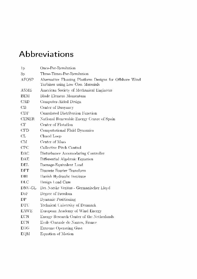
Abbreviations
1p Once-Per-Revolution3p Three-Times-Per-RevolutionAFOSP Alternative Floating Platform Designs for Oshore Wind
Turbines using Low Cost MaterialsASME American Society of Mechanical EngineersBEM Blade Element MomentumCAD Computer-Aided DesignCB Center of BuoyancyCDF Cumulated Distribution FunctionCENER National Renewable Energy Centre of SpainCF Center of FlotationCFD Computational Fluid DynamicsCL Closed LoopCM Center of MassCPC Collective Pitch ControlDAC Disturbance Accomodating ControllerDAE Dierential Algebraic EquationDEL Damage-Equivalent LoadDFT Discrete Fourier TransformDHI Danish Hydraulic InstituteDLC Design Load CaseDNV-GL Det Norske Veritas - Germanischer LloydDoF Degree of FreedomDP Dynamic PositioningDTU Technical University of DenmarkEAWE European Academy of Wind EnergyECN Energy Research Center of the NetherlandsECN Ecole Centrale de Nantes, FranceEOG Extreme Operating GustEQM Equation of Motion

x Abbreviations
FE Finite ElementFLS Fatigue Limit StateFOWT Floating Oshore Wind TurbineGA Genetic AlgorithmGDW Generalized Dynamic WakeGM Gain MarginHAWT Horizontal-Axis Wind TurbineHIL Hardware-in-the-LoopIDFT Inverse Discrete Fourier TransformIEA International Energy AgencyIEC International Electrotechnical CommissionIFE Institute for Energy Technology, NorwayIP In-PlaneIPC Individual Pitch ControlLC Load CaseLCOE Levelized Cost of EnergyLHEEA Research Laboratory in Hydrodynamics, Energetics & At-
mospheric Environment, Nantes, FranceLiDAR Light Detection And RangingLQR Linear Quadratic RegulatorLTI Linear Time-InvariantMARIN Marine Research Institute NetherlandsMBS Multibody SystemMDO Multidisciplinary Design OptimizationMIMO Multi-Input-Multi-OutputMIT Massachussetts Institute of TechnologyMOR Model Order ReductionMPC Linear Model-Predictive ControlNASA National Aeronautics and Space Administration, USANMPC Nonlinear Model-Predictive ControlNREL National Renewable Energy Laboratory, Boulder, USANTM Normal Turbulence ModelNTNU Norwegian University of Science and TechnologyNTUA National Technical University of AthensOC3 Oshore Code Comparison Collaboration

Abbreviations xi
OC4 Oshore Code Comparison Collaboration, ContinuedOC5 Oshore Code Comparison Continuation, Continued, with
CorrelationODE Ordinary Dierential EquationOL Open LoopOoP Out-of-PlanePDE Partial Dierential EquationPDF Probability Density FunctionPI Proportional-IntegralPM Phase MarginPSD Power Spectral DensityPSO Particle-Swarm OptimizationQTF Quadratic Transfer FunctionRAO Response Amplitude OperatorRGA Relative Gain ArrayRHPZ Right Half-Plane ZeroRMS Root Mean SquareRNA Rotor-Nacelle AssemblyRWT Reference Wind TurbineSID Standard Input DataSISO Single-Input-Single-OutputSLOW Simplied Low-Order Wind turbineSQP Sequential Quadratic ProgrammingSTD Standard DeviationSVD Singular Value DecompositionSWE Stuttgart Wind EnergySWL Still Water LevelTF Transfer FunctionTLP Tension Leg PlatformTMD Tuned Mass DamperTRL Technology Readiness LevelTSR Tip Speed RatioULS Ultimate Limit StateVAWT Vertical-Axis Wind TurbineZOH Zero-Order Hold

xii Abbreviations
Symbols
Greek letters
αi Angular acceleration of body i, αi ∈ R(3×1)
βp Platform pitch angular displacement (DoF)ε Strain vector for body i, εi ∈ R(6×1)
ζ Wave height amplitude, 2ζ = Hζ0(ω) Wave height complex amplitude spectrum at CFζ0(t) Incident wave height at CFη Eciencyθ Blade pitch angle (commanded)θ1 Blade pitch angle (measured, DoF)λ Wavelength (hydrodynamics)λ Scaling ratio (experimental testing)λ Tip Speed Ratio (TSR)ξk Flexible body structural damping ratio for mode kν Kinematic viscosityξ(ω) Response amplitude spectrum of generalized platform DoFs, ξ ∈ R(6×1)
ξ Damping ratioρki Flexible body i nodal reference coordinates in inertial frame, ρki ∈ R(3×1)
ρa Air densityρw Water densityσb Bending stressσ Standard Deviation (STD)σ Maximum singular valueσ Minimum singular valueτ Time constant (for real, overcritically damped poles)O Submerged volume of oating bodyξ Platform rigid-body generalized coordinates, ξ ∈ R(6×1)
ϕ Rotor azimuth angle (DoF)Φi Flexible body i shape function for translation, Φi ∈ R(3×fe,i)
ϑi Flexible body i shape function for rotation, ϑi ∈ R(3×fe,i)
ω Angular frequencyϕ Phase angleω0 Undamped natural frequency, ω0 = 2πf0
ωd Damped natural frequency (for undercritically damped poles), ωd = 2πfdΩ Rotor angular velocity (DoF) (low-speed shaft)Ωg Generator angular velocity (high-speed shaft)ωi Angular velocity of body i, ωi ∈ R(3×1)
Ωref Commanded rotor angular velocity, equal to rated value for above-rated winds

xiv Symbols
Roman letters
A Added mass coecient, A ∈ R(6×6)
A System matrix of dynamic system, A ∈ R(2f×2f)
ai Translational acceleration of body i, ai ∈ R(3×1)
ai Wave particle acceleration in direction iA∞ Innite-frequency limit of added mass coecient, A∞ ∈ R(6×6)
aw,ik Water acceleration in coordinate i of inertial system at body node kAwp Waterplane area of oating bodyB Input matrix of dynamic system, B ∈ R(2f×nu)
B Radiation damping coecient (hydrodynamics), B ∈ R(6×6)
BL,i Strain vector jacobian, linear component, BL,i ∈ R(6×fe,i)
ci Flexible body i CM in oating frame of reference, ci ∈ R(3×1)
CD,ik Quadratic Morison drag coecient in coordinate i of inertial system at bodynode k
CM,ik Morison inertia coecient in coordinate i of inertial system at body node kCA,ik Morison added mass coecient in coordinate i of inertial system at body node kC∗A,ik Modied Morison added mass coecient in coordinate i of inertial system at
body node kC∗D,ik Modied Morison drag coecient in coordinate i of inertial system at body
node kCb∗D,ik Linearized modied Morison drag coecient for damping in coordinate i of in-
ertial system at body node kCw∗D,ik Linearized modied Morison drag coecient for drag excitation in coordinate i
of inertial system at body node kCD Morison drag coecient (horizontal directions) for columns (with circular cross-
section)CD,hp Morison drag coecient (vertical direction) for heave platesC Output matrix of dynamic systemC Hydrostatic stiness matrix, dened about CF, C ∈ R(6×6)
Cmoor Mooring system overall generalized stiness about CF, Cmoor ∈ R(6×6)
cp Rotor power coecientCr,i Flexible body i inertial coupling between reference rotations and deformation,
Cr,i ∈ R(fe,i×3)
ct Rotor thrust coecientCt,i Flexible body i inertial coupling between reference translations and deformation,
Ct,i ∈ R(fe,i×3)
d Disturbance inputs to dynamic systemd Platform column spacing, distance from tower centerlineD Feedthrough matrix of dynamic systemD Morison generalized damping matrix (w.r.t SWL), D ∈ R(6×6)
De,i Flexible body i modal damping matrix, De,i ∈ R(fe,i×fe,i)
D Body diameterdt Timestep, dt = 1/fs = 1/2/fnyquistE Identity matrixE Young's modulus, modulus of elasticityf Number of MBS DoFs
Symbols xv
Faero Aerodynamic thrust force in shaft directionfe Total number of generalized elastic coordinates fe =
∑i fe,i
fe,i Number of generalized elastic coordinates of body iF i Forces acting on body i, F i ∈ R(3×1)
FMor Generalized wave forces on oating body from Morison's equation,FMor ∈ R(6×1)
Fr Froude number Fr = v/√gD
fs Sampling frequency, fs = 2fnyquistF (1) Generalized wave forces (1st order) on oating body, F (1) ∈ R(6×1)
F (2) Generalized wave forces (2nd order, slow-drift component) on oating body,F (2) ∈ R(6×1)
g Gravity constantGi Green-Lagrange strain tensor for body i, Gi ∈ R(3×3)
GvF Transfer function from rotor-eective wind speed v0 to thrust force FaeroGF see GζF
GFmor Transfer function for linearized Morison equation from incident wave elevation ζ0
to the six generalized excitation forces on the oating body, GFmor ∈ R(6×1)
GζF Force-RAO: Transfer function from incident wave elevation ζ0 to generalizedforces on oating body F wave = X, GζF ∈ R(6×1)
GvΩ Transfer function from rotor-eective wind speed v0 to rotor speed ΩGζξ RAO: Transfer function from incident wave elevation ζ0 to rigid body generalized
coordinates ξ, Gζξ ∈ R(6×1)
G Transfer function matrix, scaled.Gx see Gζx
h Water depthH System transformation matrix, H ∈ R(6×6)
H Wave height from trough to crest, H = 2ζhd,i Flexible body i discrete applied force vector, hd,i ∈ R(6p+fe×f)
he,i Flexible body i inner elastic force vector, he,i ∈ R(6p+fe×f)
hg,i Flexible body i gravitational force vector, hg ∈ R(6p+fe×f)
hhp Platform heave plate thicknesshhub Hub height (from SWL)hω,i Flexible body i quadratic velocity vector, hω,i ∈ R(6p+fe×f)
hr,i Flexible body i reaction force vector, hr,i ∈ R(6p+fe×f)
Hs Signicant wave heightI i Inertia tensor of body i, I i ∈ I3×3
Iwp Second moment of waterplane area, Iwp ∈ R(2×2)
j Imaginary unitJ Global Jacobi matrix for system-EQM, J ∈ R(6p+
∑i fe,i×f)
J Second moment of areaJ e,i Elastic body Jacobi (or selection-) matrix of body i, J e,i ∈ R(fe,i×fe,i)
J r,i Rotational Jacobi matrix of body i, J r,i ∈ R(3×f)
J t,i Translational Jacobi matrix of body i, J t,i ∈ R(3×f)
k Vector of generalized Coriolis, centrifugal and gyroscopic forces, q ∈ R(f×1)
k Wavenumber (k = 2π/λ)K Potential ow retardation function, K ∈ R(6×1)
ka Diraction parameter

xvi Symbols
KC Keulegan-Carpenter number KC = vT/DkD Morison damping factor (for uniform cylinders), kD = 1/2ρCDDKeL,i Flexible body i linear modal stiness matrix, KeL,i ∈ R(fe,i×fe,i)
kM Morison inertia factor (for uniform cylinders), kM = CMρπD2/4
kp Proportional gain (PI-controller)Li Torques acting on body i, Li ∈ R(3×1)
m Inverse slope of S/N or Wöhler curve (logarithmic x)m Body massM Global mass matrix for system-EQM, M ∈ R(f×f)
Maero Aerodynamic torque about shaft axisM e,i Flexible body i modal mass matrix, M e,i ∈ R(fe,i×fe,i)
mi Spectral moment of ith orderMyt Tower-base fore-aft bending momentN LQR weights on input-state coupling, N ∈ R(2f×nu)
Nr Reference number of cycles for DEL calculationnu Number of dynamic system inputsp Vector of generalized applied forces, p ∈ R(f×1)
p Number of bodies in MBSP Generalized damping matrix (velocity-dependent applied forces), P ∈ R(f×f)
P Electrical powerq Vector of generalized coordinates, containing the system DoFs, q ∈ R(f×1)
Q Generalized stiness matrix (position-dependent applied forces), Q ∈ R(f×f)
Q LQR weights on states, Q ∈ R(2f×2f)
r Platform column radiusR Rotor radiusRki Flexible body node k reference coordinates in oating frame of reference,
Rki ∈ R(3×1)
R LQR weights on inputs, R ∈ R(nu×nu)
Re Reynolds number Re = vD/νrhp Platform heave plate radiusri Position vector of body i, ri ∈ R(3×1)
s Laplace variableS Load range (S/N curve)S Cross product operator S (·), λ× a = S (λ)aSvv Spectrum of rotor-eective wind speed, including rotational sampling of turbu-
lenceSdd Spectrum of disturbance inputs to dynamic systemS
(1)FF Force spectrum of generalized rst order wave forces, S(1)
FF ∈ R(6×6)
S(2)FF Force spectrum of generalized second order wave forces, S(2)
FF ∈ R(6×6)
Si Rotation tensor of body i, Si ∈ R(3×3)
Syy Spectrum of response of dynamic systemSζζ Spectrum of incident wave height at the CFt Platform draftT Quadratic Transfer Function (QTF), T ∈ R(6×1)
T Complementary sensitivity function T = GK/(1 +GK)T2r Zero-upcrossing period of response
Symbols xvii
Ti Integrator time constant (PI-controller)Tlife System design lifetimeTp Peak spectral periodui Deformation eld for nodes k of body i, relative to undisplaced position,
uki ∈ R(3×1)
u Control inputs to dynamic system, u ∈ R(nu×1)
U Matrix of output directions of SVDu0 Dynamic model input operating point at system steady state, u ∈ R(nu×1)
∆u Dynamic model inputs, linearized about u0 ∈ R(nu×1)
V Matrix of input directions of SVDv0 Rotor-eective wind speed, wind disturbance input operating pointvb,ik Body velocity in coordinate i of inertial system at body node kvhub Mean wind speed at hub heightvi Translational velocity of body i, vi ∈ R(3×1)
vi Wave particle velocity in direction ivrel Relative rotor-eective wind speedvrated Rated wind speedvw,ik Water velocity in coordinate i of inertial system at body node kW i Elastic beam shape function vector, W i ∈ R(3×fe,i)
x Dynamic model states x = [q, q]T ∈ R(2f×1)
∆x Dynamic model states, linearized about x0 ∈ R(2f×1)
X Wave excitation force coecient or force- RAO, X ∈ R(6×1)
x0 Dynamic model states operating point at system steady state, x0 ∈ R(2f×1)
xp Platform surge displacement (DoF)xt Tower-top fore-aft deection w.r.t. tower-base (DoF)y Outputs of dynamic systemzII,i Kinematic function for velocity of exible body i including translation and ro-
tation of reference frame as well as elastic deformation in oating frame of ref-erence, zII,i ∈ R(6p+fe×f)
zIII,i Kinematic function for acceleration of exible body i including translation androtation of reference frame as well as elastic deformation in oating frame ofreference, zIII,i ∈ R(6p+fe×f)
zcb Distance of center of buoyancy of oating body below SWL, positive downwardszcm Distance of center of mass of oating body below SWL, positive downwardszp Platform heave displacement (DoF)


Abstract
Various existing prototypes of Floating Oshore Wind Turbines (FOWTs) demonstrate the
feasibility of placing oshore wind turbines on oating foundations, held in place by anchor
lines. The motivation of this thesis is to improve the understanding of how wind and waves
impact the dynamic behavior of semi-submersible-type platforms. The understanding of the
multi-disciplinary system shall be used to optimize the shape of the oating platforms to show
the same stable dynamics as xed-bottom ones with a resource-ecient foundation.
The thesis addresses rst the development of a dynamic simulation model with not more
than the necessary physical details. It shall bridge the existing gap between spreadsheet design
calculations and dynamic simulation models, which are used until the nal design stage and for
certication. The structural equations of motion result from an elastic multi-body system for a
reduced set of degrees of freedom. The mathematical model shall represent the overall system
dynamics without resolving the component loads. Therefore, the response is only calculated
in a two-dimensional plane, in which the aligned wind and wave forces act. Additional force
models for wind and wave forcing, as well as the mooring line forces, complete the mathematical
description. From the nonlinear system of equations a linearized model is derived. First, to be
used for controller design and second, for an ecient calculation of the response to stochastic
load spectra in the frequency-domain. A verication through a comparison against a higher-
delity model shows that the model is able to reproduce the response magnitude at the system
eigenfrequencies as well as the forced response magnitude to wind and wave excitations. The
computational eciency proves to be high with one-hour simulations completing in about 25
seconds and even less in the case of the frequency-domain model.
Through a comparison to experimental measurements in a combined wind and wave basin
at a scale of 1:60, the model validity could be conrmed. The tested concept is the TripleSpar,
a deep-drafted semi-submersible, designed as a reference in this thesis. A lesson from the ex-
periments is that a correct modeling of the hydrodynamic drag, as well as the wave forcing, is
important because these loads dominate the system response of oating wind turbines. The
coupled system stability shows to be driven by the gains of the blade-pitch controller in con-
nection with the aerodynamic and the hydrodynamic damping. Controlling the rotor speed can
destabilize the rotor fore-aft motion, while a large damping in fore-aft direction can mitigate
the problem and increase system stability.
As a result of the ndings from the experiments, the force models of the developed simulation
xx Abstract
model include a rather detailed hydrodynamic model and a simplied, ecient aerodynamic
model. The aerodynamic model computes the quasi-steady integral rotor forces as function of
the tip speed ratio and the blade pitch angle. The hydrodynamic model combines the rst-order
potential ow coecients and the viscous Morison drag, which is linearized for both, the wave
excitation and the damping forces from drag. Vertical drag at the heave plates, identied from
the measurements, compares well with data from the literature. To generally model the drag as
realistically as possible, the literature data was parameterized and used for iteratively solving
for response magnitude-dependent drag coecients. The wave radiation model is simplied
using a constant added mass, independent of the frequency. Second-order wave forces through
Newman's approximation allow a prediction of the low-frequency platform resonances. From
the frequency and time-domain models the response standard deviation, the fatigue damage
and short-term extremes are calculated.
With the obtained tailored simulation model, two parametric controllers were designed: A
new, robust proportional-integral-control design procedure results in a gain scheduling, specic
to FOWTs. It takes the stability margins at each operating point into account and thus
allows larger gains where the oating system is better damped. The controller design can be
automated and is highly independent of the platform shape as it only feeds back the rotor speed
error. For comparison, an optimal model-based state-feedback controller was designed to show
the prospect of a multi-input-multi-output controller. Results show that this controller is less
robust but improves the system fore-aft damping and allows, again, higher gains for the rotor
speed control loop.
Finally, the previously developed simulation model and the parametric controllers were ap-
plied in a brute-force optimization with parameterized design routines for the oating platform.
The optimum hull shape yields a reduction of more than 30 % of the lifetime-weighted fatigue
damage at a reasonable material cost. It is known that a good hull design can result in a
cancellation of the rst-order wave loads. However, a coupled eect could be observed for the
optimal shape: It responds to sinusoidal waves with a translation in surge and a pitching, out-
of-phase to the surge response. This means that the FOWT rotates about a point close to the
rotor hub. Consequently, the rotor fore-aft motion is almost unaected by the wave excitation.
A nal code-to-code comparison with the higher-delity model over the entire design space
was successful, yielding the same optimum as the developed reduced-order model. In order to
transfer this optimal response behavior to state-of-the-art design practices, a design indicator
was developed, which can successfully predict the optimal shape. These results show that it is
possible to design FOWTs with a very stable operational behavior. The power production and
the tower-top motion and loads are comparable to onshore wind turbines, while keeping the
size and mass of the foundation reasonably small.

Kurzfassung
Die Machbarkeit schwimmender, nur durch Ankerleinen xierter Windkraftanlagen, wurde in
den letzten Jahren durch mehrere Prototypen bestätigt. Die Motivation der vorliegenden Ar-
beit ist, das physikalische Verständnis, wie Wind und Wellen die Dynamik von Anlagen mit
Halbtaucherplattformen beeinussen, zu verbessern. Mit dem erlangten Verständnis des multi-
disziplinären Systems soll die Hüllform des Schwimmkörpers optimiert werden, um das Schwin-
gungsverhalten auf das Niveau von am Boden verankerten Oshore-Anlagen zu bringen. Dabei
sollen die Schwimmkörper möglichst ressourcenezient aufgebaut sein.
Die Arbeit beginnt mit dem Entwurf eines dynamischen Simulationsmodells, das nicht mehr
als die notwendigen physikalischen Eekte abbildet. Hiermit soll die Lücke zwischen einfachen
Tabellenkalkulationsprogrammen und komplexen dynamischen Simulationsmodellen, die bis hin
zur Zertizierung angewendet werden, geschlossen werden. Das strukturdynamische Modell ba-
siert auf einem elastischen Mehrkörpersystem mit wenigen Freiheitsgraden. Es soll die globale
Systemdynamik korrekt abbilden, ohne detaillierte Schnittlasten einzelner Komponenten aufzu-
lösen. Aus diesem Grund ist die modellierte Systembewegung auf die Ebene beschränkt, in der
Wind und Wellenkräfte wirken. Zusätzliche Untermodelle für die Berechnung der externen Kräf-
te aus Wind- und Wellenanregung, sowie der Ankerleinen vervollständigen die mathematische
Beschreibung des Gesamtsystems. Eine Linearisierung erlaubt zum einen die Anwendung linea-
rer Reglerentwurfsmethoden und zum anderen eziente Berechnungen der Systemantwort auf
stochastische Anregungen im Frequenzbereich. Der Vergleich mit einem detaillierteren Modell
hat gezeigt, dass das entwickelte Modell sowohl die Eigenschwingungen, als auch die Anregun-
gen durch Wind- und Wellenkräfte korrekt abbilden kann. Die Rechenezienz ist beachtlich,
mit Simulationsdauern von nur 25 Sekunden für die Berechnung einer einstündigen Zeitreihe
und noch kürzeren Rechenzeiten im Freqzenzbereich.
Die Gültigkeit des Modells konnte durch einen Vergleich mit experimentellen Messdaten in
einer Skala von 1:60 gezeigt werden. Das im Test verwendete Plattform-Konzept ist der Triple-
Spar, eine Halbtaucherplattform mit groÿem Tiefgang, die im Rahmen dieser Forschungsarbeit
als Referenzmodell entwickelt wurde. Die Experimente zeigen, dass eine korrekte Modellierung
des hydrodynamischen Widerstands, sowie der Wellenkräfte unerlässlich ist, da diese die Ant-
wort dominieren. Die Stabilität des schwimmenden Systems wird hauptsächlich durch die Reg-
lerkoezienten, in Verbindung mit der hydrodynamischen und aerodynamischen Dämpfung,
bestimmt. Die Drehzahlregelung neigt dazu, die Bewegung der Gondel in Längsrichtung (in

xxii Kurzfassung
Windrichtung) zu destabilisieren. Andererseits, kann eine gröÿere Dämpfung in dieser Rich-
tung die Stabilität erhöhen.
Auf Basis der Erkenntnisse aus den Experimenten wurde das Hydrodynamikmodell mit einer
groÿen Detailtiefe aufgebaut, während sich ein einfaches Aerodynamikmodell als ausreichend
erwiesen hat. Die globalen aerodynamischen Rotorkräfte sind eine Funktion der Schnelllaufzahl
und des Blattverstellwinkels. Das hydrodynamische Modell kombiniert die Koezienten des
Potenzialströmungs-Ansatzes mit dem Widerstandsterm der Morison-Gleichung. Der viskose
Widerstandsterm wird linearisiert für die Anregung und ebenso für die Dämpfung, die aus dem
Strömungswiderstand resultiert. Für eine allgemein realistischere Abbildung des Widerstands
an den Tauchplatten, wurden Daten aus der Literatur parametrisiert. Das bedeutet, dass die
Widerstandskoezienten eine Funktion der Antwortamplitude sind. Das Wellenabstrahlungs-
problem (Radiation) wurde vereinfacht durch die Verwendung einer frequenzunabhängigen hy-
drodynamischen Zusatzmasse. Wellenkräfte zweiter Ordnung sind durch die Annäherung nach
Newman modelliert und erlauben damit eine Abbildung der niederfrequenten Plattformreso-
nanzen. Aus den Frequenz- und Zeitbereichsergebnissen werden die Standardabweichung, die
Schädigungslasten, sowie die Kurzzeit-Extrema berechnet.
Mit dem erstellten Simulationsmodell wurden zwei parametrisierte Regler entworfen. Ein neu-
es Verfahren zum Entwurf eines robusten PI-Reglers erlaubt eine neue Verstärkungsplanung, die
die arbeitspunktabhängige Stabilität der schwimmenden Plattform berücksichtigt. Höhere Ver-
stärkungsfaktoren sind hier möglich bei besseren Dämpfungseigenschaften. Das Entwurfsverfah-
ren kann automatisiert und unabhängig von der Plattform angewendet werden, da es lediglich
die Rotordrehzahl zurückführt. Neben diesem wurde ein optimaler Regler mit Zustandsrückfüh-
rung entworfen, um die Vorteile eines Mehrgröÿenreglers zu zeigen. Die Robustheit des Reglers
ist eingeschränkt, allerdings erhöht er deutlich die Dämpfung in Längsrichtung.
Am Ende der Arbeit steht eine integrierte Optimierung des Schwimmkörpers unter Zuhilfe-
nahme des vorab entwickelten Modells und der beiden Regler mit parametrisierten Entwurfs-
routinen. Das Optimum zeigt eine Reduktion der gewichteten Ermüdungslasten um bis zu 30 %,
ohne Erhöhung der Materialkosten. Für Halbtaucher ist bekannt, dass die Hüllform eine Elimi-
nierung der Wellenkräfte erster Ordnung begünstigen kann. Zusätzlich wurde für die optimale
Plattform ein gekoppelter Eekt entdeckt: Das System antwortet auf harmonische Wellenan-
regung mit einer Translation in Längsrichtung und einer gegenphasigen Stampfbewegung. Das
bedeutet, dass das System um einen Punkt in der Nähe der Rotornabe rotiert und damit der
Einuss der Wellenkräfte auf den Rotor auf ein Minimum beschränkt wird. Eine Verikation der
Optimierungsergebnisse mit einem detaillierteren Modell über den gesamten Parameterraum
konnte das gefundene Optimum reproduzieren. Um die erreichte günstige Antwortdynamik im
gewöhnlichen Auslegungsprozess zu berücksichtigen, wurde ein passender Indikator entworfen.
Diese Ergebnisse zeigen, dass es möglich ist, Schwimmplattformen mit ruhigem Verhalten und
geringen Gondelbewegungen bei verhältnismäÿigem Materialaufwand zu entwerfen.

1 Introduction
Placing oshore wind turbines on oating foundations instead of bottom-xed ones has the
prospect of increasing the applicable range to sites with intermediate to deep waters, be-
yond 45 m. The idea is not new but only in recent years large-scale prototypes have been
built in a realistic environment. This shows that from a technical and logistic point of view
the concept is realizable. The technology of Floating Oshore Wind Turbines (FOWTs) is cur-
rently passing the state of being validated in relevant environment, see [1, p. 139]. However,
the free-oating foundation adds complexity to the dynamics of Horizontal-Axis Wind Tur-
bines (HAWTs) of a size currently approaching 10 MW, which are already the largest existing
rotor-dynamic systems.
This chapter gives a concise summary of the state-of-the art and the motivation of this work,
with a review of the most important previous works. The last section of this chapter introduces
the research methodology of the present thesis. A thorough introduction to the topic with the
relevant theoretical background will then be given in Chapter 2.
1.1 Motivation
Currently, the common design practice of FOWTs builds on the established methodologies for
wind turbines on the one side and the ones from oshore structures on the other side. The
current design process for xed-bottom oshore turbines was compared to oating turbines in
the paper [2] and the related project report [3]. The paper illustrates how the substructure and
the wind turbine are designed, based only on a limited exchange of parameters among the two
designers.
The consequence is a separated, component-oriented design, where the loads at the interface
are calculated using approximate models, delivered by the designer of the respective counter-
part. On the one side this means that the structural dimensioning of FOWTs follows proven
and certied procedures and the systems do satisfy all design requirements. On the other side
however, the restrictive exchange of data impedes full-system optimizations. Especially for a
novel technology as FOWTs, it is important to save costs at early design stages, because a
large portion of the upcoming lifecycle costs is being determined at the beginning of the design
process already, see [1, p. 44]. The rst out of three design stages declared by [3] includes
2 1 Introduction
mainly so-called spreadsheet calculations but no coupled simulations of the entire FOWT sys-
tem. Hence, many decisions are taken and the design is being frozen, before the full, coupled
system dynamics are considered. Therefore, new design tools of low and medium delity are
necessary to make early-stage full-system studies possible. These tools, based on simplied
dynamic models, have the advantage that they require a less detailed set of design parameters,
such that the exchange of data between two designers is less critical. The review on the FOWT
technology and markets of [1] highlights the obstacles of development due to intellectual prop-
erty and stresses the need for collaborative research. They predict a large potential for cost
reduction through technology enhancements [1, p. 143].
The goal of this work is to improve the engineering methodology for FOWT designs, which are
optimized to reject structural loads induced by wind and waves and thus, enable a smooth and
stable operation in the oshore environment. For this end, fully integrated but computationally
ecient mathematical models shall be used and the ndings will be compared to conventional
methods. The focus of this work is semi-submersible-type FOWTs and the design parameters of
interest within the integrated analysis are the oating platform hull shape and the wind turbine
controller. Since the wind turbine is usually not re-designed for the oating foundation, the
platform shape and the wind turbine controller are the components, which rstly vary most
between ongoing projects and secondly impact substantially the dynamic behavior. As a result,
the physical understanding of the dynamics of the FOWT system shall be improved and the
ndings shall be processed to be incorporated in the state-of-the-art design process.
In summary, the main research questions are:
• Numerical modeling:
Is a medium-delity simulation tool realizable to bridge the gap between spread-
sheet calculations and tools for certication?
Which are the relevant physical eects in the concept design phase?
• Design:
How to design a FOWT platform with a minimum response to wind and waves?
How much fatigue load reduction is possible through
hull shape optimization?
controller optimization?
Is an integrated FOWT system optimization necessary instead of a sequential one?
Are there new design indicators which outperform conventional ones?
Design indicators refer to quantities, which can be used as cost functionals for conceptual design
calculations. They are expected to indicate optimal system properties before detailed design
calculations are conducted.
After the review of related research in the next section, the specic goals, the methodology
and the scope of the present study will be outlined.

1.2 Related Work 3
1.2 Related Work
Several works were performed before the research on this thesis started in 2013 on reduced-
order modeling, control design and integrated optimization. With the rst conceptual designs
of FOWT platforms, studies were made already on the dierences of the dynamic behavior
with the goal of gaining more insight into the driving physics. First approaches for numerical
simulations and an evaluation of dierent concepts was made as early as 2000 in the thesis by
Henderson [4]. The rst generic concepts were developed at Massachussetts Institute of Tech-
nology (MIT) in 2006 with a comparison between concepts with taut versus catenary mooring
lines under supervision of Sclavounos [5]. Around 2010, a thorough numerical analysis compar-
ing three types of oating platforms was carried out at National Renewable Energy Laboratory,
Boulder, USA (NREL) and the University of Stuttgart by Jonkman and Matha, see [6]. Sev-
eral studies applying optimization algorithms to FOWT platforms were done afterwards for
spar-type platforms [7], for Tension Leg Platforms (TLPs) [8] and for a design space spanning
dierent types [9].
The critical inuence of the blade pitch controller for the FOWT dynamics was reported rst
in [10] with further studies in [11] and [12]. The rst parametric design study including the
wind turbine controller was done in [8] on TLPs. The distinct inuence of the controller in the
design process, however, has not yet been analyzed.
Reduced-order numerical FOWT models, necessary for system analysis and optimization,
have been developed in 2011 by [13] for spar-type platforms including aerodynamic loads and
a bit later by [14] for the same type but specically for control design purposes. The basis for
state-of-the-art numerical FOWT modeling, however, with a clear preparation of the hydrody-
namic time-domain modeling techniques, adopted from oshore engineering, and wind turbine
aero-servo-elasticity was provided by Jonkman [15].
The thesis by Lupton [16] of the University of Cambridge, UK, focuses in detail on lineariza-
tion approaches for FOWT modeling, which enables fast spectral methods for load calculations.
As in this work, a numerical model was developed using Lagrange's equation for the multibody
system description. The subsystems of aerodynamic, hydrodynamic and mooring line forces
and the controller were linearized separately applying two dierent methods. Additionally, an
approximation of the second-order hydrodynamic forces was investigated. The work showed
in a comprehensive way how linearization techniques can be applied to a system as complex
as a FOWT, where nonlinear eects play a non-negligible role for various load cases. In sum-
mary, the work has provided a good understanding of the potential of linearized formulations
of the dierent submodels. Also, the coupled FOWT response was investigated in realistic
environmental conditions but it is stated that further work is needed for a practical application
of the code due to limitations in the operating range of the wind turbine, the description of
the environmental conditions (deterministic vs. stochastic), the platform type and the compu-

4 1 Introduction
tational eciency. Several ndings and derivations of [16] strengthen the present work, such
as the frequency-domain calculations and the linearization of the hydrodynamic drag. The
work provides important ndings for the present simulation model, especially regarding the
frequency-domain hydrodynamics.
The thesis by Bachynski [8] of the Norwegian University of Science and Technology (NTNU)
has a comparable structure as the present one as it extends existing simulation models for the
dynamic analysis of various TLP-type oating wind turbines. For the dierent developed TLP
platforms, in-depth numerical analyses were performed with realistic load cases, used for cer-
tication, including controller fault cases. A large part of the work addresses second-order
and third-order hydrodynamic forcing with an assessment of the importance of such forces for
the considered TLPs. Nonetheless, a reduced-order model is also developed and compared to a
state-of-the art aerodynamic model, coupled to a structural model. Although Bachynski focused
on another FOWT-type than the present work, the numerical modeling approaches are com-
parable, including linear frequency-domain methods, the inclusion of the controller (although
not platform-dependent) and higher-order hydrodynamic models.
1.3 Aim and Scope
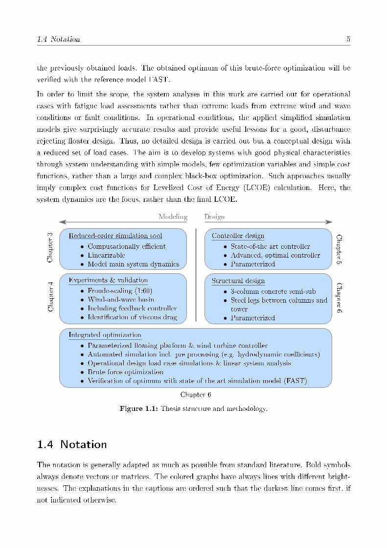
The methodology and outline of this thesis is shown in Figure 1.1. On the modeling side, a
new simulation model will be presented in Chapter 3, which is tailored to the specic research
questions. The computational eciency will allow for many load case simulations and extensive
sensitivity studies. Only the main system dynamics shall be modeled without a representation
of the component response. A linearization allows for linear system analyses, rst of all for
controller design but also to improve the understanding of the system behavior, which depends
on the operating point and on the system parameters with and without the controller.
The developed model will be veried through experimental tests in a combined wind and wave
basin, including the controller, in Chapter 4. With the measurement data the hydrodynamic
drag will be identied and subsequently a validation of the assumptions taken for the model
derivation is carried out.
Two model-based controllers will be developed for an automated controller design in Chap-
ter 5. They are a baseline controller and an advanced controller, in order to assess their dier-
ences but also their eect on dierent platform hull shapes. The controllers will be applied in
an integrated optimization study.
A design space of the platform hull shape will be dened in Chapter 6 with the goal of running
an optimization and sensitivity studies. Design routines for the structural dimensioning as
function of the hull shape will be developed. This leads to the integrated design load simulations
of the fully parameterized system and linear system analyses to improve the understanding of
1.4 Notation 5
the previously obtained loads. The obtained optimum of this brute-force optimization will be
veried with the reference model FAST.
In order to limit the scope, the system analyses in this work are carried out for operational
cases with fatigue load assessments rather than extreme loads from extreme wind and wave
conditions or fault conditions. In operational conditions, the applied simplied simulation
models give surprisingly accurate results and provide useful lessons for a good, disturbance
rejecting oater design. Thus, no detailed design is carried out but a conceptual design with
a reduced set of load cases. The aim is to develop systems with good physical characteristics
through system understanding with simple models, few optimization variables and simple cost
functions, rather than a large and complex black-box optimization. Such approaches usually
imply complex cost functions for Levelized Cost of Energy (LCOE) calculation. Here, the
system dynamics are the focus, rather than the nal LCOE.
Modeling Design
Reduced-order simulation tool
• Computationally ecient• Linearizable• Model main system dynamics
Experiments & validation
• Froude-scaling (1:60)• Wind-and-wave basin• Including feedback controller• Identication of viscous drag
Controller design
• State-of-the art controller• Advanced, optimal controller• Parameterized
Structural design
• 3-column concrete semi-sub• Steel legs between columns andtower
• Parameterized
Chapter3
Chapter4
Chapter
5Chapter
6
Integrated optimization
• Parameterized oating platform & wind turbine controller• Automated simulation incl. pre-processing (e.g. hydrodynamic coecients)• Operational design load case simulations & linear system analysis• Brute-force optimization• Verication of optimum with state-of-the-art simulation model (FAST)
Chapter 6
Figure 1.1: Thesis structure and methodology.
1.4 Notation
The notation is generally adapted as much as possible from standard literature. Bold symbols
always denote vectors or matrices. The colored graphs have always lines with dierent bright-
nesses. The explanations in the captions are ordered such that the darkest line comes rst, if
not indicated otherwise.

2 Background
This chapter provides the necessary theory and a literature review on oshore wind energy and
oating wind energy with a comparison of dierent FOWT platform types and integrated design
approaches. Subsequently, the specic dynamics of FOWTs are discussed, followed by linear
frequency-domain modeling techniques, the environmental conditions for load simulations and
scaled experimental testing approaches, before an introduction into the wind turbine control
system, especially for FOWTs, is presented. The chapter terminates with the specication of
a reference oater for a 10 MW wind turbine, which is developed as a baseline for all of the
following studies.
2.1 Oshore Wind Energy
The Paris Agreement of the United Nations on climate change, which entered into force in
2016, has marked a turning point in the goal of reducing global warming, it has been ratied
by 184 states at the time of publication of this thesis. Societal eorts on a large scale favor
sustainable trac, industry and power production, triggering global trends such as the Di-
vestment Movement, which attracts more and more global players to stop their investments in
fossil power generation. Public policy regulates the market by introducing measures such as the
European Emission Trading System or dierent subsidy systems by national governments. The
multidisciplinary interconnectedness of the energy transition is a challenging project, especially
when it comes to leaving behind traditional industries. The renewable electricity market shows
complex dynamics, above all in the times of renewable energy exceeding the demand. Notwith-
standing these challenges, with the Paris Agreement the transition to renewable energy was
for the rst time regarded by the media as having a potential of being economically protable,
which is a proof of the technological achievements in the renewable energy sector as well as the
development of more ecient machinery. Nonetheless, the research of this thesis shall not be
seen as a manifesto for high-tech solutions to the current challenges of humankind but rather
as one piece of a manifold of necessary measures, with, above all, societal changes.
According to [17] more than 50 % of the installed power capacity in Europe can be attributed
to wind energy. Wind energy overtook coal, which used to be the second largest form of power
generation in 2016. The installed capacity is higher than that of hydroelectric power and
8 2 Background
about 50 % larger than that of solar power. The outlook for 2030 by WindEurope (former
EWEA) [18] predicts in its central scenario an installed capacity oshore of 66 GW compared
to 12.4 GW in 2016 [17]. In terms of the energy mix, currently about 10 % of Europe's energy
production stems from wind, of which about 12 % is produced oshore [17]. The International
Energy Agency (IEA) predicts in its World Energy Outlook [19] a portion of 40 % of the total
power generated worldwide to come from renewables by 2040. This shows the large potential
of oshore wind as a technology but also as a mature and expanding industry. While in
Germany, as the nation with the largest installed wind capacity in Europe (44 % [17]), the
market growth will slow down for onshore wind, there is a large potential oshore. The overall
installed capacity oshore in Europe grew between 2002 and 2012 from less than 100 MW to
1100 MW [20]. In 2012 about 75 % of oshore wind turbines were installed on xed-bottom
Monopile foundations but [20] predicts that the market of deeper waters is increasing exploring
water depths of more than 200 m. In such depths, xed-bottom foundations are no longer
feasible. Floating platforms can be alternatives in these locations.
2.2 Floating Oshore Wind Energy
To date, the rst prototype tests of FOWTs were successfully completed, such as Statoil's
Hywind spar with a 2.3 MW turbine [21], Principle Power's WindFloat [22], with a 2 MW
turbine and the Japanese project Kabashima with a 2 MW turbine on two dierent platform
types. Currently, various demonstration projects are running and rst commercial projects are
under way such as the Hywind Scotland project, the Kincardine and Dounreay oating wind
farms, also in Scotland, with a total of almost 100 MW. The WindFloat Atlantic o the coast
of Portugal will comprise 25 MW and a French project of 100 MW is planned with four dierent
oating platform concepts in two construction phases. Recently, a British and an Irish project
were announced with 1.5 GW, each. An overview of technologies and current projects can be
found in [23], [24] and [25].
Floating wind turbines can be distinguished from other oshore turbines through the criterion
that no rigid structural connection to the sea oor exists as is the case for xed-bottom foun-
dations such as Monopiles, gravity foundations and jackets. The denition by [26] highlights
the vertical force from buoyancy as unique feature of FOWTs.
2.3 Comparison of Platform Types
The technologies can be grouped into ballast-stabilized, buoyancy stabilized and mooring-
stabilized systems. The rst, called spar, feature a rather large draft with mostly a slender
cylindric shape and a keel lled with ballast. Here, the large gravitational force, far below
2.3 Comparison of Platform Types 9
the Still Water Level (SWL), ensures the static stability. For buoyancy-stabilized systems,
called barge, a large volume at the water surface yields increased buoyancy forces where the
volume displaces more water, which in turn results in static stability, see Figure 2.1a. This type
of platform usually features a low draft with a large breadth. Currently, several concepts are
being developed which are hybrids between a spar and a barge, meaning that they receive the
static stability from both, buoyancy and gravity. These are called semi-submersibles, see Fig-
ure 2.1b, 2.1c. Most ongoing projects work with semi-submersible-type concepts, of which [27]
provides a general overview.
The systems with taut moorings, called TLP, are stabilized by the mooring lines, pulling the
platform body with excess buoyancy below the water surface such that a large pre-tension exists
in the lines. Due to the taut lines and a little amount of ballast this type of platform is lighter
than the other oaters and has higher eigenfrequencies of the substructure. It is therefore stier,
in vertical direction almost comparable to xed-bottom platforms, see [28]. Consequently, the
system eigenfrequencies of the TLP substructure are usually above the wave frequency range.
This is not the case for the types with slack lines, where the horizontal translation mode can
be far below the peak spectral frequency of the waves.
In the literature, a number of comparative studies can be found on the dierent FOWT
concepts. The previously mentioned early studies by Sclavounos are summarized in the overview
paper [5]. The authors have shown that, based on frequency-domain hydrodynamic modeling
and a simplied representation of the wind turbine, a small dynamic response can be achieved
either with a shallow-drafted barge or a spar on the other hand. Matha and Jonkman [6],
however, highlighted the large response of barges compared to semi-submersibles and TLPs, in
line with the ndings by Robertson [29]. However, the latter studies did not consider parameter
variations of the hull shape, in contrast to [5]. The studies show that especially the section
forces close to the sea surface, are higher for FOWTs than for onshore turbines, due to the wave
loads.
The European research project LIFES50+1 brings together four designers of dierent plat-
form types (2 semi-submersibles, 1 barge, 1 TLP) with three universities and three research
institutes in order to upscale the existing concepts and increase the Technology Readiness Level
(TRL) to a value of 5, meaning that the technology development of the designs is completed,
including experimental testing. This project fosters technology transfer from research to indus-
try and provides an important platform for the exchange of knowledge of the dierent elds
involved in oshore wind energy. The concepts with slack mooring lines are shown in Figure 2.1.
This platform type is is the focus of this thesis and parts of the presented results were generated
within LIFES50+.
1http://lifes50plus.eu/, accessed on January 22, 2018.

10 2 Background
(a) Ideol barge (b) Nautilus semi-submersible
(c) OlavOlsen OO-StarWind Floater semi-
submersible
Figure 2.1: Ballast- and buoyancy-stabilized FOWT concepts of the project LIFES50+,photographs courtesy of the designers.
2.4 Optimization and Systems Engineering
Design optimization is a topic in engineering which has been addressed extensively in the lit-
erature, especially challenging are multi-disciplinary systems such as FOWTs. Currently, the
concept of Systems Engineering is being introduced to wind turbine design (IEA task 372),
mainly focusing on the aero-elastic design, see [30, 31]. Both of these examples use a Sequential
Quadratic Programming (SQP) algorithm. Systems Engineering has its origins at the National
Aeronautics and Space Administration, USA (NASA) for aerospace applications and has the
main objective of integrating a multidisciplinary design process. As a result, components are
not designed independently but taking into account the coupling eects on the entire system.
For a comprehensive realization of the Systems Engineering principles, integrated, multidisci-
plinary design tools are necessary, with various interfaces between the dedicated tools for a
single discipline. The methodology is called Multidisciplinary Design Optimization (MDO).
In this work, a multidisciplinary numerical model is used for a design optimization through
a simultaneous variation of the parameters of the wind turbine controller and the platform
dimensions. Whereas MDO studies usually aim at the reduction of the overall lifetime cost, in
this work the cost function is reduced to fatigue loads and the power uctuation. Hence, the
main goal is to optimize the dynamic behavior.
Optimization algorithms were already applied to traditional oshore structures. An example
for a parametric design model of oil and gas support structures subject to optimization for
a reduced downtime through improved seakeeping is given in [32]. Here, a complex potential
2http://windbench.net/iea37, accessed on January 11, 2018.

2.5 Dynamics of Floating Wind Turbines 11
ow model was parameterized, comparable to the present work. A rst approach for integrated
design of xed-bottom oshore turbines was presented in 2004 in the thesis by Kühn [33].
Later, various studies were published, especially for jackets, where the lattice structure was
optimized. Examples are [34], applying a Particle-Swarm Optimization (PSO) algorithm, [35]
with a Genetic Algorithm (GA) and [36] using a gradient-based optimizer. With the latter
it is especially important to ensure a continuous description of the cost function, which is not
possible with complex functions and usually not feasible for MDO. For Monopiles, a recent risk-
based optimization was presented in [37]. A summary of various optimization algorithms and
an application to mechanical systems using multibody approaches and symbolic programming,
as in the present work, can be found in the thesis [38].
For FOWTs several optimization studies were described already in Section 1.2. One study,
resembling MDO techniques to the largest extent is published in [9]. It includes the hull shape
and mooring line design across dierent platform types using a genetic algorithm. In that work,
a frequency-domain model is derived from the code FAST v7 [39], with a linear representation
of the hydrodynamic viscous damping but without representing the wind turbine controller.
The genetic algorithm is applied for single- and multi-objective optimization. The results show
dierent, rather unconventional, designs, which might indicate that a renement of the cost
function is necessary, according to the author. A rst brute-force optimization with tailored
blade-pitch controllers was performed in the course of the present research and was presented
in [40].
2.5 Dynamics of Floating Wind Turbines
While for conventional oshore oil and gas structures the wave loads are dominant and the wind
loads are only approximated by static forces [41], this approach is not possible for FOWTs:
Dynamic simulations with a representation of the wind turbine aero-elasticity are necessary
in order to capture the dynamic response correctly and to ensure that the structure does not
show resonances leading to large loads and excursions. For FOWTs, structural elasticity is
important due to the slenderness of the tower and the blades and needs to be considered for
design calculations. The aerodynamic forces depend on the blade section local inow angle
of attack. Therefore, the integral rotor forces depend on the wind speed, the rotor speed and
the blade pitch angle. Since the blade pitch angle is an actuated variable of the wind turbine
control system, next to the generator torque, the controller dynamics also need to be taken into
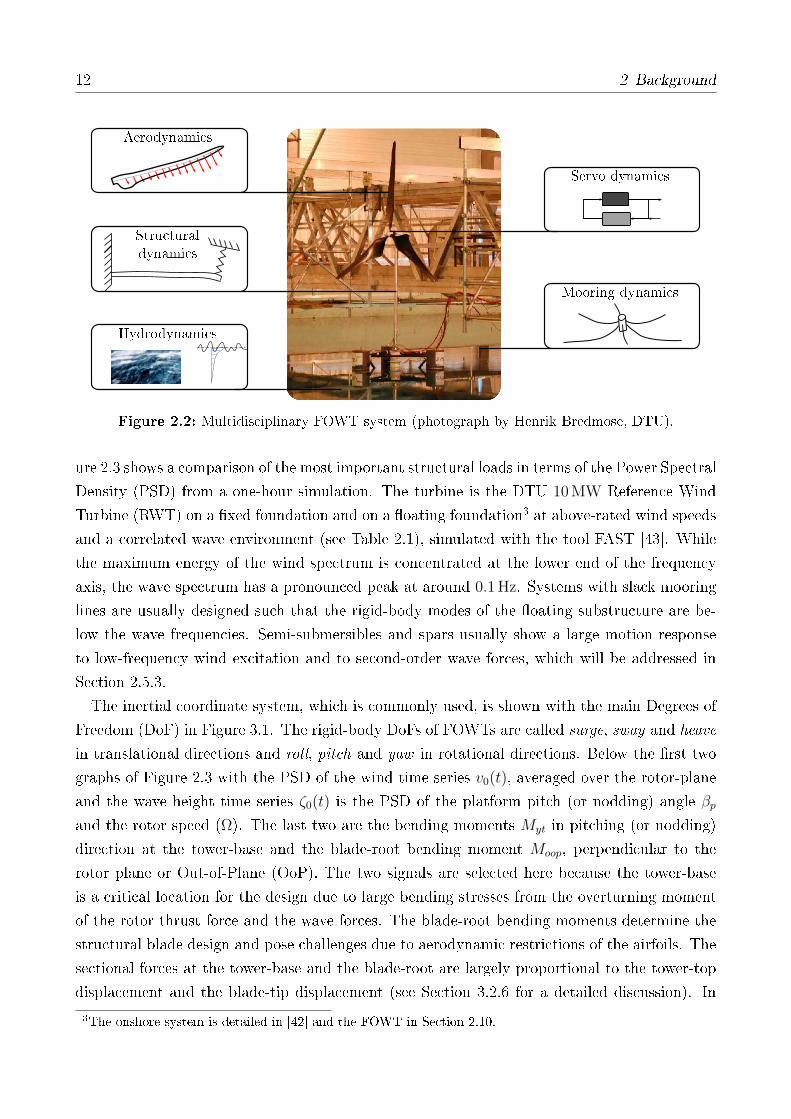
account. This results in a multidisciplinary system as illustrated in Figure 2.2.
The purpose of this section is to give an introduction to the main system dynamic character-
istics of FOWTs and available methods for numeric simulations, looking rst at the structural
dynamics and subsequently at the aerodynamics, hydrodynamics and mooring dynamics. Fig-
12 2 Background
Aerodynamics
Hydrodynamics
Servo dynamics
Mooring dynamics
Structuraldynamics
Figure 2.2: Multidisciplinary FOWT system (photograph by Henrik Bredmose, DTU).
ure 2.3 shows a comparison of the most important structural loads in terms of the Power Spectral
Density (PSD) from a one-hour simulation. The turbine is the DTU 10 MW Reference Wind
Turbine (RWT) on a xed foundation and on a oating foundation3 at above-rated wind speeds
and a correlated wave environment (see Table 2.1), simulated with the tool FAST [43]. While
the maximum energy of the wind spectrum is concentrated at the lower end of the frequency
axis, the wave spectrum has a pronounced peak at around 0.1 Hz. Systems with slack mooring
lines are usually designed such that the rigid-body modes of the oating substructure are be-
low the wave frequencies. Semi-submersibles and spars usually show a large motion response
to low-frequency wind excitation and to second-order wave forces, which will be addressed in
Section 2.5.3.
The inertial coordinate system, which is commonly used, is shown with the main Degrees of
Freedom (DoF) in Figure 3.1. The rigid-body DoFs of FOWTs are called surge, sway and heave
in translational directions and roll, pitch and yaw in rotational directions. Below the rst two
graphs of Figure 2.3 with the PSD of the wind time series v0(t), averaged over the rotor-plane
and the wave height time series ζ0(t) is the PSD of the platform pitch (or nodding) angle βpand the rotor speed (Ω). The last two are the bending moments Myt in pitching (or nodding)
direction at the tower-base and the blade-root bending moment Moop, perpendicular to the
rotor plane or Out-of-Plane (OoP). The two signals are selected here because the tower-base
is a critical location for the design due to large bending stresses from the overturning moment
of the rotor thrust force and the wave forces. The blade-root bending moments determine the
structural blade design and pose challenges due to aerodynamic restrictions of the airfoils. The
sectional forces at the tower-base and the blade-root are largely proportional to the tower-top
displacement and the blade-tip displacement (see Section 3.2.6 for a detailed discussion). In
3The onshore system is detailed in [42] and the FOWT in Section 2.10.

2.5 Dynamics of Floating Wind Turbines 13
Figure 2.3, the platform pitch mode at 0.025 Hz is clearly visible in the third plot, and this
is reected in the tower-base loads (fth plot). Even more signicant is the response of the
tower-base moment from rst-order wave loads at the wave frequency at 0.1 Hz and slightly
above. Another distinct dierence is the low-frequency response of the rotor speed to wind
excitations: The FOWT controller allows larger amplitudes than the onshore turbine. This is
due to the fact that the controller gains have to be de-tuned (reduced) for FOWTs to ensure
the system's stability if only standard control schemes are applied. Section 2.9 will give an
introduction into the controller for FOWTs. The blade moment (lower plot) shows a distinct
response at the Once-Per-Revolution (1p) frequency at 0.16 Hz and a response to the turbulent
wind eld but only a slight excitation from the wave loads. Remarkable is that the 1p-frequency
is more dominant for onshore turbines than for the oating counterpart. A possible reason is
the shifted modal properties due to the oating substructure.
onshore
floating
frequency [Hz]
bld
Moop
[MN
m2/H
z]
twrM
yt
[GN
m2/H
z]
rot-
spd
[rpm
2/H
z]
ptf
mpit
ch
[deg
2/H
z]
wave
[m2/H
z]
win
d
[m2/s2
/H
z]
0.1 0.2 0.3 0.4 0.5 0.6 0.7
0
500
0
0.050
5
0
10
20
0
10
20
0
50
Figure 2.3: Comparison of responses of DTU 10 MW RWT onshore and oating at vhub = 17.9 m/s.
A distinct feature of FOWT dynamics is the coupling between the platform pitch motion
response with the rotor response. This is due to the relative, or apparent, rotor-eective wind
speed (the one that the rotor sees). A coupling to the controller-induced dynamics appears,
since the rotor speed responds to these changes in the relative wind speed and, in turn, the
controller reacts to the rotor speed error. The surge-direction is usually not as important

14 2 Background
for FOWTs as the pitch mode because it has generally a lower eigenfrequency, which is better
damped.
Numerical modeling of FOWTs has large overlaps with the methods of the oshore oil and
gas industry, as mentioned above. One major dierence is that fatigue analyses are highly
important for wind turbines, due to the persistent harmonic excitation [44]. For a structural
fatigue assessment, a representative probability distribution of load cycle amplitudes is neces-
sary and this requires extensive numerical simulations. First fatigue calculations were made
in the frequency-domain, due to the lower computational eort, see e.g. Dirlik [45]. The
calculation of the dynamic wave forcing on vertical piles was presented as early as 1965 by
Borgman [46]. Due to the multi-disciplinarity of FOWTs the complexity of numerical mod-
els increases signicantly and as a consequence, rst oshore wind farms were designed using
de-coupled numerical predictions of the structural stresses. With the increase of comput-
ing power, linear frequency-domain analyses for dynamic simulations were slowly replaced by
computationally demanding nonlinear time-domain simulations. In oshore wind, so-called
multi-physics models are common where dierent dedicated software tools run simultaneously.
Here, the Equations of Motion (EQM) are not set up as a whole but the tools solve their
own EQM and exchange states and forces in each timestep. Dedicated wind turbine models,
so-called aero-elastic modeling tools, predict the wind turbine loads and dedicated tools for the
wave-structure interaction determine the hydrodynamic forcing. Dierent coupling schemes
for FOWTs are described in [26]. A study on the validity of a superposition of the loads at
e.g. the tower-base, coming from wind and wave loads can be found in [47] and in a recent
study [48]. The rst approaches to integrated analyses of (xed-bottom) oshore wind turbines
were made as part of the theses by Kühn [33] and later by van der Tempel [49]. More details
on fatigue calculation will be given in Section 2.6 and 2.7.
For FOWTs, the rst modeling tools were developed by Henderson [4]. Later, Jonkman [15]
provided a detailed description of the theory behind the rst and only available open-
source FOWT simulation tool FAST [43] by NREL, which is used as a reference in this work.
A general overview on FOWT modeling can be found in the recently published book [50]. To
date, a variety of mostly commercial simulation tools for FOWTs exist, among others Simpack
by Dassault Systèmes, Bladed by Det Norske Veritas - Germanischer Lloyd (DNV-GL), Hawc2
by Technical University of Denmark (DTU) and 3DFloat by Institute for Energy Technology,
Norway (IFE). Various other commercial codes exist, in addition to a number of in-house re-
search codes by universities and research organizations. An extensive code comparison project
was performed within IEA task 23 and task 30, namely the projects Oshore Code Comparison
Collaboration (OC3), Oshore Code Comparison Collaboration, Continued (OC4) and Oshore
Code Comparison Continuation, Continued, with Correlation (OC5) where a large number of
institutions participated worldwide, running simulations on xed-bottom and oating wind
turbines for various load cases. The results for FOWTs are published in [51, 52, 53, 54]. Other
2.5 Dynamics of Floating Wind Turbines 15
studies reviewing and comparing the predictions of dierent simulation approaches can be found
in [55, 56, 57] and in the LIFES50+ project report [58].
The next sections will give an overview on the FOWT subsystem dynamics, the structural
dynamics, aerodynamics, hydrodynamics and the mooring line dynamics and the respective
modeling methods and available simulation tools. Further details are part of the reduced-model
derivation in Chapter 3.
2.5.1 Structural dynamics
As shown above, oshore wind turbines show large deections of the tower and the blades as
response to the environmental loads. Therefore a Multibody System (MBS) approach is usually
implemented in the structural modeling tools. High-delity Finite Element (FE) models can
be applied for the exible components of the wind turbine while the formulation of the MBS
accounts for the large reference motion with a correct physical representation of the kinetics of
inertial, Coriolis, centrifugal and gyroscopic forces.
In many simulation tools such as FAST, the exible bodies, mainly the rotor blades and the
tower, are simplied through a Model Order Reduction (MOR) and represented in the exi-
ble MBS through a limited number of shape functions following a Ritz approach, see [59]. These
shape functions are commonly the mode shapes of the respective bodies, obtained through an
eigenanalysis using FE models. Although individual shape functions are dened for each body,
they should not be calculated without representing the rest of the coupled system. The Rotor-
Nacelle Assembly (RNA) inertial mass, for example, needs to be accounted for when calculating
the tower shape functions. The number of necessary mode shapes to be included is usually based
on engineering judgment. In state-of-the-art aero-elastic simulation codes, at least the rst two
modes in fore-aft and side-side direction are used, giving four exible DoFs of the tower. For
the blades made of ber reinforced epoxy, the mode shapes are more complex: If the blade
cross-section is approximately symmetric it can be assumed that the principal axes are aligned
with the blade chord, a function of the radius, see [60]. Therefore, the rst bending mode
shapes are twisted with the blade principal axis in FAST. The most important mode shapes
are normally selected as the rst two apwise modes (about the soft axis) and the rst edge-
wise mode (about the sti axis) giving a total of nine DoFs for the rotor. Especially for
large blades or for aero-elastic stability analyses, higher modes and at least one torsional mode
needs to be included because torsion changes the local angle of attack and consequently the
aerodynamic forces and moments, see [61] and recently [62] with a validation of the simulation
code FAST with full-scale measurements.
The oating platform is modeled as a rigid body in FAST with six DoFs if all directions
are unconstrained. Studies were made recently to include the substructure exibility in the
dynamic system analysis. This has mainly the objective to obtain the structural stresses within
16 2 Background
the substructure, which is not possible with state-of-the-art tools. An approach calculating the
stresses as a post-processing of the time-domain results of a state-of-the-art model was presented
rst for Bladed [63] and by NTNU in [64]. In [65] and [66], the exibility was also considered
in the uid-structure interaction problem.
Additional DoFs of the state-of-the-art FOWT models are the rotor rotation, the drive-
train torsion and the blade pitch actuator model DoFs, usually represented by a second-order
dynamic system, giving four additional DoFs. While the blade pitch actuator model is not
included in FAST and has to be included in a custom Simulink model, the yaw drive actuator
is included through a rotational spring-damper element. This yaw drive actuator represents
another additional DoF.
All of the mentioned DoFs can be activated in FAST resulting in a total of 25 DoFs. The
reduced-order model derived in Chapter 3 considers only a planar platform motion in the
vertical 2D plane and neglects the exibility of the blades in order to focus on the main system
dynamics. The structural model, however, is built with the theory of exible MBS, as described
above. The EQM will be derived in Section 3.2.
2.5.2 Aerodynamics
Common state-of-the-art wind turbine simulation codes represent the loading from aerodynam-
ics usually through Blade Element Momentum (BEM) theory. Momentum theory is the part
describing the deceleration of the ow across the rotor due to the momentum imposed by the
rotor on the steady ow. The other part of BEM theory is the blade element theory, which
gives the local forces on each blade section with a discrete width and chord, given an angle of
attack and airfoil polar data. This involves an iteration because blade element theory requires
the angle of attack, which comes from the momentum theory. The result of this iteration is the
induction factor, giving the local velocities in the rotor plane based on the simulation input,
the 3D turbulent wind eld, see Section 2.7, far upstream and undisturbed by the rotor. Only
with the local induction factor, the wind speeds at the rotor plane can be determined and the
local forces are calculated using the blade polars. A derivation of the standard BEM-theory
can be found in [60].
The basic BEM theory involves many assumptions: First, the rotor is discretized through
annuli, each having a constant induction. This means one can imagine the rotor as a disk. The
assumption of discrete annuli implies that there is no dependence of the ow in radial direction,
which is especially critical for yawed inow, see [44, Chapter 3]. Another simplication is related
to the root and the tip losses, which occur due to shed vortices, which reduce the circulation
at these blade sections. The authors of [44] state that this radial dependence of the induction
violates the BEM assumptions as it yields a radial exchange of momentum. However, for
common operating points, the assumption of radial independence of annular forces is said to

2.5 Dynamics of Floating Wind Turbines 17
be reasonable. Other assumptions include no special consideration for the situation of heavily
loaded rotors under large induction factors, where a recirculation of the ow at the outer radius
of the disc occurs, denoted as vortex ring state and, more severe, the turbulent wake state.
Important for control design purposes might be the fact that quasi-steady aerodynamics are
assumed, meaning that a stepwise change in the angle of attack yields an instantaneous response
of the forces, e.g. [67]. This is not the case for a real rotor as several aerodynamic phenomena
yield a dynamic response of the forces. These can be grouped into three categories, see [68]
or also [26] and [69]: First, local airfoil dynamic eects, causing a circulation lag, also called
Theodorsen Eect a phenomenon happening in attached ow conditions. Second, for large
angles of attack stall occurs reducing the lift and increasing the drag through shed vortices.
Considering unsteady changes in the angle of attack the shed vortices, traveling over the blade
chord, yield the dynamic stall phenomenon. Apart from these local eects, the third eect is
related to the global ow through the rotor disc. It cannot be assumed to behave in a quasi-
steady manner, mainly because the ow has to accelerate or decelerate, which cannot happen
instantaneously, due to the inertia of the ow. This dynamic inow or dynamic wake eect
causes a delay in the blade forces following a change of, e.g., the blade pitch angle in attached
ow conditions.
The computational scheme of BEM theory has proven to be very ecient compared to other
methods. Therefore, a variety of correction models has been developed. An important one is,
according to [44] and [60], the hub and root loss correction model. This model accounts for the
above-mentioned vortices shed at the blade segments at the root and the tip. Correction models
to the mentioned dynamic eects of the aerodynamic forces are the dynamic stall and dynamic
inow model. The Glauert correction for large induction factors accounts for the re-circulation
eect. The correction of the 2D airfoil data from experiments or potential ow simulations
for 3D ow situations is usually done in a pre-processing step. The spreadsheet tool [70] is an
example of how to prepare the airfoil data for BEM tools with a 360 range of angles of attack
and the correction of eects from a rotating blade, rather than static airfoils. A good review
of BEM models including corrections can be found in [71]. A thesis on possible corrections
based on experimental analyses can be found in [72].
For FOWTs, especially unsteady aerodynamics can be important in certain ow situations.
Although this work focuses on simplied conceptual models, some of these are listed here for a
better understanding of the underlying physics of real wind turbine rotors. Recently, a number
of studies was made for moving rotors due to the oating foundation. The application of the
dynamic inow correction models for FOWTs is described in [73]. It shows the importance
of the time scale of the frequency of the oating platform, compared to the unsteady aerody-
namics. It showed that BEM theory-based models are generally valid for FOWT modeling.
The importance of the frequency of oscillation of the oating platform has also been investi-

18 2 Background
gated by the authors of [74]. Their approaches will be discussed further in the results chapter,
Section 6.4.6.
Alternatives to BEM include the second theory implemented in the reference model FAST.
Besides BEM-theory it includes the Generalized Dynamic Wake (GDW) model, which is based
on the Pitt and Peters dynamic inow model, see [68], but it includes higher-order terms than
the common correction model to BEM theory, see [75]. It is still considered an independent
aerodynamic model because, even in steady conditions, the modeling is dierent than with BEM
models: The pressure distribution along the blade is modeled through Legendre functions, which
include the above mentioned tip and root losses. One case in Chapter 6 uses this model. A
theory guide of the aerodynamic model AeroDyn of FAST can be found in [76].
Higher-delity models are potential ow approaches as the Lifting Line and Free-Wake Vor-
tex Method, which models the wake together with the uid-structure interaction problem. The
thesis [77] gives a good description of the method. Its application to FOWTs can be found
in [78] and [79]. As in helicopter theory, especially the interaction of the rotor with its wake
can be better represented with these models. Even more complex Computational Fluid Dy-
namics (CFD) models have been applied to FOWTs in [80, 81, 82, 83, 84], showing reasonable
results but a challenging implementation and signicant computational eort. The project Of-
fwindtech went further, studying the dierent aerodynamics due to the oating foundation and
the consequences of the moving hub condition for blade design with the goal of reducing loads
and increasing the power production, see [85]. That work had a comparable objective of the
one of this thesis as variations of the design are investigated in order to adapt current concepts
better to the oating foundations with the goal of reducing loads and therefore less material
usage in the construction.
For this work, simplied, computationally ecient and linearized aerodynamic models are nec-
essary for control design and design optimization. Several approaches exist here, the simplest
being the modeling of the entire rotor as a disk with overall aerodynamic coecients depending
on the Tip Speed Ratio (TSR) and the blade pitch angle, which will be described in Section 3.4.
Other simplied models avoid the discretization of the blade and the time-consuming iteration
to nd the induction factor through overall aerodynamic blade coecients and a representative
blade-eective wind speed, but still including a dynamic inow model, see [69]. According
to [86] the above-mentioned vortex methods can also be simplied for control applications.
An extensive work on linearized, reduced-order aero-elastic modeling for controller design, was
presented in [87]. A simplied dynamic inow representation is given in [67] with an order re-
duction of the structural and aerodynamic states (considering dynamic inow) based on shape
functions.
2.5 Dynamics of Floating Wind Turbines 19
2.5.3 Hydrodynamics
In this section, an introduction will be given to state-of-the-art hydrodynamic FOWT modeling
and the methods for hydrostatic and hydrodynamic FOWT design. Besides the available text-
books on oshore hydrodynamics, the book section [88] provides an overview on hydrodynamic
modeling of oshore wind turbines, including FOWTs.
Hydrostatics
Archimedes' principle of buoyancy results in static forces on the wetted surface of a FOWT,
including position-dependent restoring forces. These restoring forces are important for the static
stability of FOWTs and represent a constraint for the dimensioning. Analytical expressions for
simple shapes make an approximation of the hydrostatic properties in spreadsheet calculations
possible. The hull shape determines important parameters like the submerged volume, the
center of buoyancy, which is the center of the submerged volume, and the cross-sectional area
of the body at the water surface, the waterplane area Awp [89]. The restoring stiness in vertical
heave direction can be obtained with the water density ρw and the gravity constant g as
C33 = ρwgAwp. (2.1)
The hydrostatic restoring stiness C55 is responsible for withstanding the aerodynamic thrust
force under a limited pitch angle βp. It depends on the second moment of the waterplane area
I22,wp =
∫∫
Awp
x2dxdy. (2.2)
With the submerged volume O and the structural mass m, the restoring stiness in pitch is
C55 = ρwgI22,wp + ρwgOzcb −mgzcm. (2.3)
Platforms with a small waterplane area usually have a low center of gravity zcm, positive in
upward direction. The gravitational forces and the buoyancy forces, acting on the center of
buoyancy zcb, result in a restoring moment, contributing to C55. For symmetric bodies C44 =
C55. The linear stiness matrix C ∈ R(6×6) needs to be augmented with restoring forces from
the mooring system. For unmoored bodies, all entries but the above-mentioned ones are zero.
Ocean waves
Ocean waves require dierent levels of complexity of their mathematical description, depending
on their nonlinearity. Linear surface waves have a sinusoidal prole, while steeper waves have
larger troughs and shorter crests. Dierent theories exist to model the wave kinematics in time

20 2 Background
and space. Usually, potential ow theory is employed with dierent orders of nonlinearity of the
free surface boundary condition, see [89, p. 75] for a visualization of the dierent regimes. Linear
waves can be modeled in a straightforward manner such that the uid kinematics over depth can
be solved for by hand if no obstacles in the domain are considered, see e.g. [90, p. 5-12]. Linear
waves travel with the phase speed vp, a function of the wave frequency. This means that the time
series at dierent locations cannot simply be shifted in time. The dispersion relation represents
the link between the time and the spatial dimension of linear waves. It is transcendental but it
can be simplied for deep waters with a depth-to-wavelength ratio h/λ > 1/2 [90, p. 5-2]. The
deep water approximation gives the phase speed
vp =1
2
√g
k=
1
2
√gλ
2π, (2.4)
where k denotes the wavenumber, see [91, Chapter 6.2]. With deep water approximation, the
wavenumber results from the wave angular frequency ω as k = ω2/g.
Using linear wave theory, the complex amplitude spectrum of the incident wave elevation ζ(ω)
at dierent locations along the wave heading direction x can be obtained through the factor
fx(x, ω) = eikx. (2.5)
With this factor, the time series ζx(t) at the new location result from the amplitude spectrum at
the original location ζ0(ω) ≡ ζ(ω, x=0) in a discrete-time notation for a dataset of N elements
as
ζx(t) =1
N
N−1∑
ωi=0
fx(x, ωi)ζ0(ωi)e2πωit
N . (2.6)
Numerical toolboxes provide functions for the Inverse Discrete Fourier Transform (IDFT) such
that
ζx(t) =1
Nidft (fx(x)ζ0(ω)) . (2.7)
The wave kinematics over depth z can now be calculated in the frequency-domain from the
amplitude spectrum ζ0(ω). The water particle velocity in horizontal and vertical directions
are necessary for the calculation of the wave forces through Morison's equation, Section 2.5.3.
Throughout this work, we take advantage of deep water approximation, introduced earlier in
this section, and the wave heading direction is always aligned with the global x-coordinate.
The horizontal and vertical velocities over depth z result as
vx(ω, x, z) = ωζ(ω, x)ekz (2.8)
vz(ω, x, z) = jωζ(ω, x)ekz. (2.9)
2.5 Dynamics of Floating Wind Turbines 21
Consequently, the horizontal velocity is in phase with the instantaneous free-surface eleva-
tion ζ(ω, x) ∈ C, while the vertical velocity is 90 deg ahead of the free-surface elevation. The
water particle acceleration can be written as
ax(ω, x, z) = jω2ζ(ω, x)ekz (2.10)
az(ω, x, z) = −ω2ζ(ω, x)ekz. (2.11)
If obstacles are present in the computational domain, e.g. xed or oating bodies, the di-
mensions of the body determine the characteristics of the wave-induced forcing. Potential ow
panel codes, which include the body in the domain, can model eects from diraction (of the
waves around the oating body) as well as the forces from radiated waves acting back on the
body. Viscous loads, on the other side, are entirely neglected by potential ow theory. This is
the strength of empirical Morison's equation, addressed later in this section. Morison's equa-
tion, however, assumes a transparent body, meaning that the wave eld is not aected by the
body and diraction eects are neglected.
Figure 2.4 shows the ocean wave domains as function of the nondimensional characterization
of the forcing on a body in waves. The rst dimensionless number on the horizontal axis is
the diraction parameter ka, the product of the wavenumber k and the body radius a = D/2.
It can be alternatively expressed with the wavelength λ as ka = πD/λ. On the vertical axis
is the Keulegan-Carpenter number, which is the product of the uid velocity amplitude v and
the wave period T , divided by the signicant length D [90, p. 12-16]. Alternatively, KC can
be obtained from the water particle excursion x, or, in a simplied manner, from the wave
height H as
KC =vT
D= 2π
x
D≈ π
H
D. (2.12)
The wave breaking limit H/λ = 1/7, simplied for the case of deep water waves, is shown in
Figure 2.4 as function of KC and ka [90, p. 13-4]. It is not dependent on the dimensions of the
body. The location of the scaled model parameters and Load Cases (LCs) of Chapter 4 and
the LCs used for the parametric design in Chapter 6 are marked in the gure. Acceleration-
dependent inertial forces are the dominant ones for small KC . Velocity-dependent drag forces
become more important for larger KC . Consequently, a FOWT spar will experience a larger
portion of drag forces in a given sea state than a deep water oshore structure of large diameter.
The large diameter will also yield a larger diraction parameter ka and thus more signicant
wave diraction. The simulation model should be set up accordingly and consider hydrody-
namic coecients from a panel code or include an additional diraction correction model, when
Morison's equation is used. In general, a limit of ka = 0.5 is given in [92, p. 174], above which
the diraction eect is important. Both, potential ow theory, as well as Morison's equation
will be introduced for frequency-domain and time-domain computations.
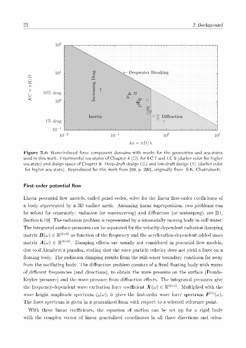
22 2 Background
← Deepwater Breaking
Incr
easi
ng
Dra
g
→
DiffractionInertia
ka = πD/λ
KC
=πH/D
10−2 10−1 100 10110−1
1% drag
100
10% drag
101
102
Figure 2.4: Wave-induced force component domains with marks for the geometries and sea-statesused in this work. Exprimental sea states of Chapter 4 (), for LC 7 and LC 9 (darker color for highersea state) and design space of Chapter 6: Deep-draft design (4) and low-draft design (O) (darker colorfor higher sea state). Reproduced for this work from [89, p. 290], originally from S.K. Chakrabarti.
First-order potential ow
Linear potential ow models, called panel codes, solve for the linear rst-order coecients of
a body represented by a 3D surface mesh. Assuming linear superposition, two problems can
be solved for separately: radiation (or maneuvering) and diraction (or seakeeping), see [91,
Section 6.19]. The radiation problem is represented by a sinusoidally moving body in still water.
The integrated surface pressures can be separated for the velocity-dependent radiation damping
matrix B(ω) ∈ R(6×6) as function of the frequency and the acceleration-dependent added mass
matrix A(ω) ∈ R(6×6). Damping eects are usually not considered in potential ow models,
due to d'Alembert's paradox, stating that the wave particle velocity does not yield a force on a
oating body. The radiation damping results from the still-water boundary condition far away
from the oscillating body. The diraction problem consists of a xed oating body with waves
of dierent frequencies (and directions), to obtain the wave pressure on the surface (Froude-
Krylov pressure) and the wave pressure from diraction eects. The integrated pressures give
the frequency-dependent wave excitation force coecient X(ω) ∈ R(6×1). Multiplied with the
wave height amplitude spectrum ζ0(ω), it gives the rst-order wave force spectrum F (1)(ω).
The force spectrum is given in a generalized form with respect to a selected reference point.
With these linear coecients, the equation of motion can be set up for a rigid body
with the complex vector of linear generalized coordinates in all three directions and orien-
2.5 Dynamics of Floating Wind Turbines 23
tations ξ ∈ R(6×1) as
ξ =[xp, yp, zp, αp, βp, γp
]T, (2.13)
see also [91]. For the reduced-order models developed in this work, only the 2D-motion in
the xz-plane is considered and ξ reduces to
ξ =[xp, zp, βp
]T, (2.14)
see also Eq. (3.1), related to the reduced order model derivation. The equation of motion is
− ω2 [M +A(ω)] ξ + jωB(ω)ξ +Cξ = X(ω)ζ0(ω) = F (1)(ω), (2.15)
with the structural mass matrix M . With Eq. (2.15), the Response Amplitude Operator
(RAO) ξ(ω)/ζ0(ω) can be calculated, the transfer function from the wave height ζ0 to the
rigid-body generalized coordinates ξ.
The above-mentioned separation of radiation and diraction is convenient for a linear FOWT
description. The matrices A(ω) and B(ω) represent the system properties, whereas X(ω)
stands for the external forcing on the right-hand side of the EQM.
Frequency-to-time-domain transformation
FOWTs are usually simulated in time-domain to obtain extreme and fatigue loads while ac-
counting for a transient motion of the oating body. These transients can arise from wind-
induced motion, transmitted through nonlinear force models, including the wind turbine con-
troller. Therefore, Eq. (2.15) needs to be transformed into time-domain, which was achieved
by Cummins, see [93]. Important is the mathematical description of the forces from radiated
waves, resulting from a transient body motion. The dynamics of the bulk of uid particles
surrounding the hull are given in the frequency-domain by
K(ω) = B(ω) + jω [A(ω)−A∞] . (2.16)
The retardation function K(ω) is the sum of a real part, the damping coecient, and the
imaginary dierence of the added mass and its innite-frequency limit A∞. The transfer
function from a body motion to the resulting forces from radiated waves can be obtained from
the uid impulse response function K(t). Ogilvie [94] realized a time-domain description of
Eq. (2.16), by transforming its real part or the imaginary part as
K(t) =2
π
∫ ∞
0
B(ω) cos(ωt)dω = − 2
π
∫ ∞
0
ω [A(ω)−A∞] sin(ωt)dω. (2.17)

24 2 Background
Consequently, the impulse response function K(t) is available from the rst-order panel code
coecients A(ω) and B(ω).
With the impulse response function K(t), the generalized radiation forces can be written,
according to Cummins, as function of the generalized body acceleration ξ and velocity ξ with
a convolution integral
F rad(t) = −A∞ξ(t)−∫ t
0
K(t− τ)ξ(τ)dτ. (2.18)
Cummins' equation is the complete time-domain EQM, including the radiation forces of
Eq. (2.18)
(M +A∞)ξ(t) +
∫ t
0
K(t− τ)ξ(τ)dτ +Cξ(t) = F (1)(t). (2.19)
It is commonly implemented in state-of-the-art oating wind simulation tools like FAST, see [95]
and others. The exciting forces F (1)(t) on the right-hand side of Eq. (2.19) are usually obtained
through an IDFT of a complex force spectrum F (1)(ω). Alternatively, a transfer function can
be tted to the dynamics from wave height ζ0 to the generalized forces F (1). The convolution
integral of Eq. (2.19) is numerically demanding because a time history of platform states has
to be kept in the memory for the integration over times τ . Also here, a transfer function can
be tted to avoid this problem. These approaches are subject of the next section.
In summary, Eq. (2.19) has several important properties. Firstly, the added mass, or the
forces in phase with the body acceleration, depend on the body frequency of oscillation. Thus,
the eigenvalue problem needs to be iterated, as discussed in [96]. Secondly, the damping force,
due to the dissipated energy with the radiated waves, depends on the frequency of oscillation.
For many FOWT types, this linear radiation damping is small compared to the viscous damping
through shed vortices. This will be discussed in more detail in the Section 3.5.
Parametric dynamic models
The above EQM in frequency-domain, Eq. (2.15), and in time-domain, Eq. (2.19), are both
based on numerical transfer functions, due to the hydrodynamic coecients, A(ω), B(ω) and
X(ω) from the panel code, but they are not parametric equations in the Laplace domain. In
this section, an alternative is presented, which is especially useful for the controller design of
Chapter 5. The term parametric means here a Linear Time-Invariant (LTI) model with a
nonzero number of states in the case of a state-space model, or poles, in the case of a linear
transfer function. The coecients of these models are parameterized such that the new LTI
model represents the best t to the original model from the panel code through methods of
system identication. The advantage of these models is mainly that the complete time-domain

2.5 Dynamics of Floating Wind Turbines 25
dynamics are described as a unied, parametric system with a general form
x = Ax+Bu
y = Cx+Du.(2.20)
The state vector is denoted by x, the input vector by u and the output vector by y. Such a
model has been applied for control-oriented representations of oating systems, especially in
order to avoid the convolution integral of Eq. (2.19). In this case, the tted dynamic model
of Eq. (2.20) represents the dynamics from platform position to the radiation forces on the
platform. Such LTI models for the radiation problem were proposed in [97] and [98] for wave
energy converters and in [99] and [100] for vessels with the description of the corresponding
Matlab toolbox in [101]. The method of a tted state-space model has been applied to oating
wind turbines and incorporated in the FAST model [39], in [102]. It is therefore possible to
directly compare the performance of coupled time-domain simulations of oating wind turbines
using Cummins' equation with the tted LTI radiation model.
Also the wave excitation force coecientX(ω), part of Eq. (2.19), can be subject to a system
identication for an LTI model. As part of the research on this thesis, the theory provided in [97]
was applied to two FOWT platforms in [103]. The original model with the heave-DoF, only was
extended to the surge and pitch-direction for the non-cylindric shapes of a semi-submersible.
The input to this dynamic wave force model is the incident wave height ζ0. This is a more
intuitive input than the hydrodynamic forces F (1), which are the inputs in other models. The
new method is especially advantageous for the set up of parametric transfer functions, either of
the plant (from system inputs u to outputs y, or system states x) or from a disturbance (wave
height ζ0 to outputs or system states). These disturbance models are important for the design
of controllers like Dynamic Positioning (DP) control [104] for vessel stabilization and distur-
bance rejection. Here, a slow feedback control attenuates the excitations from second-order
drift forces on oshore supply vessels. For the complex dynamics of FOWTs, such disturbance
rejection methods are important, see e.g. [105] for structural control using Tuned Mass Dampers
(TMDs), [106] and [107] for nonlinear and linear model predictive control and [108] for feed-
forward control. Feedforward control is seen as a promising application of the wave model of
this work since a better system description together with advanced wind and wave sensors can
help to reduce fatigue and also extreme loads. The parametric wave excitation model will be
included in the reduced-order model development in Chapter 3.
Morison's equation
Morison developed a semi-empirical force model for the wave forces on slender vertical
piles [109]. It has been extended for oating bodies and has a number of practical advantages
over Cummins' equation. Morison's equation gives the horizontal force ∆F on a cylindrical sec-

26 2 Background
tion or strip i in the normal directions k of the body surface with diameter D and length ∆l.
The force is a function of the undisturbed uid accelerations aik and the velocities vik. The
Morison forces in the two horizontal directions in the inertial frame are given by
∆Fik∆l
= kMaik + kD vik|vik| (2.21)
with
kD =1
2ρwCDD and kM = CMρwπ
D2
4. (2.22)
Several parallels are present between Cummins' equation (2.19) and Morison's equation (2.21).
The inertia coecient CM can be obtained from the added mass coecient CA as CM = 1 + CA.
In Eq. (2.21), no body motion is yet considered such that the rst summand represents the
Froude-Krylov wave forces, represented by F (1) in Eq. (2.19). The Froude-Krylov wave forces
from Morison's equation are equal to the panel code results for low frequencies, where diraction
is negligible, with CA = 1, see [92]. Both coecients, for drag CD, and added mass CA, need
to be obtained from experiments or from the literature, e.g. [110]. For simple shapes, the zero-
frequency limit A0 of the added mass coecient from the panel code can be used as a reference
as shown in [111] and [112].
An extension of Morison's equation has been made for moving bodies [113]. Additional to
the undisturbed wave kinematics, the oating body velocity vb,ik and their derivatives vw,ikand vb,ik determine the external Morison force
vik = vw,ik − vb,ik and aik = vw,ik − vb,ik. (2.23)
Thus, the Froude-Krylov forces and the radiation added mass forces are represented, as in
Cummins' equation, Eq. (2.19). The uid kinematics are usually calculated as explained in Sec-
tion 2.5.3 assuming hydrodynamically transparent structures, neglecting diraction eects.
In Morison's equation, the acceleration-dependent force (rst part of Eq. (2.21)) is indepen-
dent of the frequency. This simplication is valid for slender cylinders, which experience little
radiation forces.
The semi-empirical nature of Morison's equation oers several advantages. No pre-
computation of the hydrodynamic coecients A(ω), B(ω) andX(ω) of Eq. (2.19) with a panel
code is necessary. As a consequence, the distributed forces over the body axial coordinate can
be obtained. This is not generally possible with Cummins' equation, because the panel code
pre-processor integrates the pressures over the wetted surface. With the distributed pressures,
the deformation and the structural stresses of the oating platform can be calculated. This is
only possible through a post-processing with Cummins' equation, as discussed in Section 2.5.1.
Additionally, the quadratic drag force is considered in Morison's equation, which is neglected
by the panel code.
2.5 Dynamics of Floating Wind Turbines 27
Many of the widespread FOWT simulation codes combine Cummins' equation with Mori-
son's equation. The advantage of Cummins' equation with the panel code coecients is that
diraction is generally considered such that no restriction on the body dimensions, like the col-
umn diameter-to-wavelength ratio D/λ, is present. This is especially important for the FOWT
types barge and semi-submersible. The quadratic viscous drag forces, however, are not part of
Cummins' equation. This is the reason why the drag force component of Eq. (2.21) is often
added as additional component to Cummins' equation (2.19) as shown in [53]. Morison's equa-
tion has also been extended for vertical directions, which is important for semi-submersibles
with heave plates. A vertical drag force is here necessary to model, see [112]. The importance
of the vertical drag forces of heave plates will be discussed in more detail in Chapter 3 and
Chapter 4.
For the present model, a linearization of Morison's equation is necessary for the frequency-
domain model. It will be described in Chapter 3 on the simplied simulation model. The
nonlinear drift loads at low frequencies will be introduced next.
Second-order slow-drift forces
The discussed wave force transfer function X(ω) of Eq. (2.15) is a linear description. As will
be discussed in Section 2.8, experimental tests have shown that non-negligible wave forces
outside the frequencies of the free-surface elevation ζ0 appear for FOWTs. These forces result
mathematically from nonlinear eects, especially from the free-surface boundary condition.
With the quadratic boundary condition, regular waves exert a steady mean drift load on a
vertical wall in the wave propagation direction, which is not the case if linear potential ow
is applied. The theory of mean drift and slow drift forces is well explained in the lecture
notes [114]. The same model, solved for a bichromatic wave, includes forces which are out
of the range of their own frequency. The forces appear at the sum and the dierence of
the two wave frequencies. The resulting force transfer function has two frequencies as input
and is therefore called a Quadratic Transfer Function (QTF). The low-frequency force (at the
dierence frequency) may coincide with the system eigenfrequencies and yield large amplitudes
of motion of the oating body and large stresses in the mooring system, see [115]. Thus, the
drift force has a frequency lower than the two input waves and therefore the force spectrum
contains energy where the wave height spectrum does not contain any energy. The same eect
is known from acoustics. The so-called beat pattern arises from the interference of two waves
of close frequencies. These two waves sum up to a resulting wave with an envelope of a low
frequency, also called bounded long waves, see [90].
The physical eects included in second-order potential theory are, as opposed to linear po-
tential ow: (1) the integration of the forces up to the instantaneous waterline and (2) the
nonlinear boundary condition at the free surface (Bernoulli equation with quadratic dynamic

28 2 Background
pressure, e.g. [89, p. 48]). Two numerical options are available to calculate the second-order
potential. The more ecient one is the fareld solution, based on the momentum equation. It
gives, however, only translational forces. The other option is a pressure integration over the
oating body wetted surface. This option is called the neareld solution.
In [116] and [117] the phenomenon of second-order potential ow forces coming from sum and
dierence frequencies on FOWTs were analyzed and compared among dierent computational
codes. They showed that especially the dierence frequency component can yield platform
resonances. A comparison of slow drift forces with aerodynamic forces for the OC3 spar [111]
was made in [118] and it was shown that the energy of the motion response due to slow drift
forces is of smaller magnitudes than the aerodynamic force. In [119] the slow drift forces
were parametrically calculated for a xed cylinder with a simplied approach showing that
the response magnitude is a function of the platform diameter. Especially for large diameter
structures (oshore oil and gas industry), a large response is to be expected for large waves.
Analyses for FOWTs on TLPs were presented in [120] and [121] showing that the slow drift
is of less importance for FOWTs with taut moorings, although it is noted in [8] that the
sum-frequency forces are important for the prediction of vertical motions and tendon tensions.
Many of the studies also mention that the eect of aerodynamic damping is of importance when
rating the signicance of second-order forces and therefore the controller dynamics, idling cases
or cases of misaligned waves can be critical. The possibility to include second-order potential
ow forces in time-domain FOWT simulations was added to FAST in version 8, see [95].
In this work, Newman's approximation is implemented in the simulation model. It is a
simplication in order to avoid the calculation of the full Quadratic Transfer Function (QTF).
Especially for the comparisons with the experiments of Chapter 4, these forces are important
and will be analyzed in more detail.
2.5.4 Mooring dynamics
As for the previously described submodels of aerodynamics and hydrodynamics, also the moor-
ing lines, responsible for the station-keeping of the FOWTs, can be modeled with dierent
delity levels. The major dierence among the widespread models is the static or dynamic
description: Static mooring line models predict the section force in the line or at the an-
chor/fairlead as a function of its position only. Dynamic models include also velocity and
acceleration-dependent eects such as the mooring line inertial mass, added water mass and
damping through vortex shedding.
A detailed analysis comparing static and dynamic models for all three types of FOWTs was
carried out in the thesis by Azcona [122]. It could be shown that usually the fatigue loads in
the line itself are highly aected by the mooring model type and to a lesser extent the wind
turbine and rotor loads. The same author concluded in [123] that the tower-base fatigue loads
2.6 Linear Frequency-Domain Modeling 29
are also aected by the mooring model for TLPs and to a lesser extent for semi-submersibles,
mostly the portion of the tower-base bending moment in side-side direction. These general
ndings were conrmed in a comparison of dierent models with experimental data [124].
Several numerical tools are available for mooring line simulations like the ones integrated
into FAST, the quasi-static MAP++ model [125] and the dynamic model MoorDyn [126],
which both allow the modeling of multi-segmented lines. Another dynamic mooring line model
is the one developed in Simpack, see [26, 127] and Opass, veried through experiments in [128].
A study on dierent available methods for the derivation of the equations of motion for dynamic
models can be found in [129]. Due to the nonlinearity of mooring line forces, higher-delity
models are necessary for the computation of extreme mooring tensions for FOWTs in storm
conditions, where slack line events can happen, yielding large ultimate loads. A study on such
load conditions can be found in [130]. For linear frequency-domain analyses, the mooring line
properties are usually linearized such that the mooring line restoring forces on the platform are
represented by a 6 × 6 stiness matrix. For the reduced-order model developed in this work,
a quasi-static model is implemented due to its computational eciency and its suitability for
linearization, see Chapter 3.
2.6 Linear Frequency-Domain Modeling
As mentioned at the beginning of Section 2.5, linear frequency-domain methods had been used
for oshore oil and gas and wind turbine modeling before computing power increased signi-
cantly in the last 15 years and the attention goes more towards nonlinear high-delity models.
However, for the purpose of this work with large parametric studies and dynamic system anal-
yses, linear frequency-domain modeling is highly advantageous. Even the full load response
to a stochastic environmental excitation can be computed eciently through a multiplication
of transfer functions. Especially in ocean engineering such methods are advantageous because
the external loads from waves and wind are stochastic in nature. In the frequency-domain,
the power spectrum Sxx(ω) can be calculated numerically with a Discrete Fourier Transform
(DFT) of the stationary stochastic process x(t). The stationarity means that the expected
value E[x(t)] and E[x(t)x(t+ τ)] are both independent of the time t. The complex amplitude
spectrum x(ω) results from the discrete DFT, normalized with the number of elements N of
the frequency vector, as
x(ω) =dft(x(t))
N, (2.24)
where N includes also negative frequencies in the Fourier space. Thus, x(ω) is a two-sided
amplitude spectrum, which is consequently half the magnitude of the one-sided amplitude
spectrum. In the Laplace domain, no negative frequencies exist but the transient dynamics are
covered by the complex Laplace variable s, while the frequency variable in Fourier space is the
30 2 Background
real angular frequency ω. With a Single-Input-Single-Output (SISO) state-space model with
system matrix A, input vector b and output vector c, the linear transfer function G(jω) in the
imaginary Laplace domain can be calculated with the identity matrix E
G(jω) = cT (jωE −A)−1b. (2.25)
The PSD, the response auto-spectrum is dened as
Sxx(ω) =dt
N|dft(x(t))|2 = dtN |x(ω)|2 . (2.26)
In oshore wind turbine analyses, the wind and wave disturbances can be described as spectra
of stochastic processes, dened in standards such as [131], which will be detailed in Section 2.7.
A good introduction to stochastic processes and spectral methods is given in [46] and the
references therein. For a Multi-Input-Multi-Output (MIMO) system G(ω), the response auto-
spectrum Syy(ω) to the matrix Suu(ω) of the input spectra is simply given by the multiplication
Syy(ω) = G∗T (ω)SuuG(ω), (2.27)
where G∗T (ω) denotes the complex conjugate transpose. The argument ω covers positive
frequencies ω > 0 and therefore the PSD is single-sided. The imaginary unit of the Laplace-
domain frequency axis will be omitted for the calculation of response spectra. From a power
spectral density Sxx(ω), the standard deviation σ or Root Mean Square (RMS) can be calculated
from the zeroth spectral moment m0 using Parseval's theorem by numerically integrating over
the positive frequencies
σ =√m0 =
√∫ ∞
0
|S1sddxx (f)| df. (2.28)
Therefore, no integration or time-stepping as in time-domain methods is necessary for solving
the Ordinary Dierential Equation (ODE) of the state-space model, which can save orders of
magnitude of computational time. The large amount of simulation time necessary for calcu-
lating a sucient number of load cycles of all relevant frequencies for fatigue load estimation
makes time-domain simulations challenging, see [132] for a good elaboration of fatigue design
methods for wind turbines. This is why these ecient methods reappeared recently in oshore
wind simulation studies, see [16, 69, 133, 134]. A selection of published frequency-domain sim-
ulation tools for wind turbines includes the tool Turbu by the Energy Research Center of the
Netherlands (ECN) described in [135] and Hawc2Stab by DTU, see [136].
For wind turbines, the dependency of the system dynamic properties on the azimuth angle
of the rotor presents a challenge for the frequency-domain modeling. This is usually handled
through the transformation of the states dened in the rotating frame into the non-rotating
2.7 Environmental Conditions and Load Calculation 31
frame. An application of this Coleman transformation can be found in [69]. In the same
reference also the challenges arising from nonlinearities of the aerodynamic forces are discussed.
One of these cases is when the ow is not anymore attached to the airfoil and stall occurs, see
Section 2.5.2. For large rotor blades, also structural nonlinearities play a signicant role such
that linear beam model might not always be sucient as was discussed in Section 2.5.1.
For hydrodynamics, nonlinearities occur if steep or braking waves are modeled or when
considering the nonlinear potential ow problem (quadratic free-surface boundary condition),
see Section 2.5.3. Next to the wave model, the forcing model is also of importance. The
linearization of the viscous drag is a challenging task. This is discussed in detail in Chapter 3.
Linear models are only valid to represent nonlinear physics, where a small change of ∆x
about an operating point x0 occurs. These nonlinearities have to be considered with respect to
the phenomenon being analyzed. In summary, frequency-domain methods are very useful for
conceptual design calculations, optimizations and for applying linear control design methods,
where an understanding of the overall system properties is important. The linear model used
in this work will be derived in Chapter 3.
2.7 Environmental Conditions and Load Calculation
The structural loads are usually the response quantity of interest for limit-state design, where
the Ultimate Limit State (ULS) can be a design driver but, especially for wind turbine compo-
nents, also the Fatigue Limit State (FLS). Additionally, also displacements and accelerations
can be a constraint, e.g. the maximum blade tip deection or the maximum acceleration at the
nacelle. This section will introduce the characteristics of wind and waves and their modeling.
Eventually, a simplied set of Design Load Cases (DLCs) will be dened and the principles of
load calculation and requirements for the design.
2.7.1 Wind
The wind can be modeled either as a deterministic time-dependent function or as a random
stochastic process. For stochastic load simulations, the mean wind speed is constant in time
periods between 10 min to 60 min. The uctuating component is determined by the turbulence
spectrum, where the standard deviation σx in the longitudinal direction is dened for the Normal
Turbulence Model (NTM) by the IEC [131] as
σx = Iref (0.75vhub + b) . (2.29)
The expected value of the turbulence Iref at 15 m/s depends on the class the turbine is designed
for. In this work, the lowest turbulence class (C) is used due to the reduced turbulence at sea.
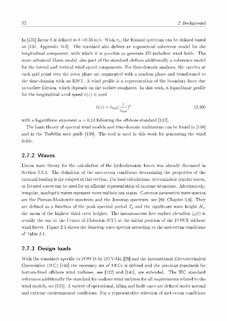
32 2 Background
In [131] factor b is dened as b =0.56 m/s. With σx, the Kaimal spectrum can be dened based
on [131, Appendix B.2]. The standard also denes an exponential coherence model for the
longitudinal component, with which it is possible to generate 3D turbulent wind elds. The
more advanced Mann model, also part of the standard, denes additionally a coherence model
for the lateral and vertical wind speed components. For time-domain analyses, the spectra at
each grid point over the rotor plane are augmented with a random phase and transformed to
the time-domain with an IDFT. A wind prole is a representation of the boundary layer due
to surface friction, which depends on the surface roughness. In this work, a logarithmic prole
for the longitudinal wind speed v(z) is used
v(z) = vhub(z
zhub)α (2.30)
with a logarithmic exponent α = 0.14 following the oshore standard [137].
The basic theory of spectral wind models and time-domain realizations can be found in [138]
and in the TurbSim user guide [139]. The tool is used in this work for generating the wind
elds.
2.7.2 Waves
Linear wave theory for the calculation of the hydrodynamic forces was already discussed in
Section 2.5.3. The denition of the met-ocean conditions determining the properties of the
external loading is the subject of this section. For load calculations, deterministic regular waves,
or focused waves can be used for an ecient representation of extreme situations. Alternatively,
irregular, stochastic waves represent more realistic sea-states. Common parametric wave spectra
are the Pierson-Moskowitz spectrum and the Jonswap spectrum, see [89, Chapter 5.8]. They
are dened as a function of the peak spectral period Tp and the signicant wave height Hs,
the mean of the highest third crest heights. The instantaneous free surface elevation ζ0(t) is
usually the one at the Center of Flotation (CF) at the initial position of the FOWT without
wind forces. Figure 2.5 shows the Jonswap wave spectra according to the met-ocean conditions
of Table 2.1.
2.7.3 Design loads
With the standards specic to FOWTs by DNV-GL [28] and the International Electrotechnical
Commission (IEC) [140] the necessary set of DLCs is dened and the previous standards for
bottom-xed oshore wind turbines, see [137] and [141], are extended. The IEC standard
references additionally the standard for onshore wind turbines for all requirements related to the
wind models, see [131]. A variety of operational, idling and fault cases are dened under normal
and extreme environmental conditions. For a representative selection of met-ocean conditions
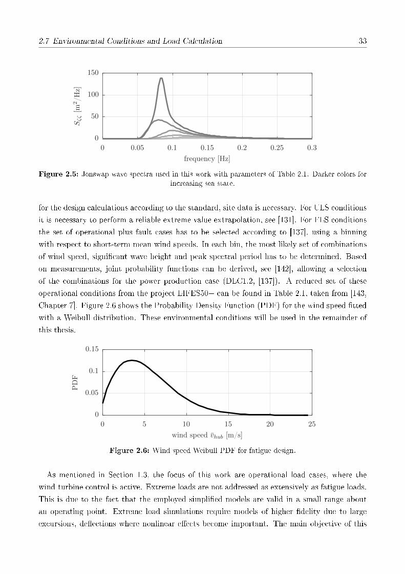
2.7 Environmental Conditions and Load Calculation 33
PSfrag replacements
frequency [Hz]
Sζζ[m
2/H
z]
0 0.05 0.1 0.15 0.2 0.25 0.3
0
50
100
150
Figure 2.5: Jonswap wave spectra used in this work with parameters of Table 2.1. Darker colors forincreasing sea state.
for the design calculations according to the standard, site data is necessary. For ULS conditions
it is necessary to perform a reliable extreme value extrapolation, see [131]. For FLS conditions
the set of operational plus fault cases has to be selected according to [137], using a binning
with respect to short-term mean wind speeds. In each bin, the most likely set of combinations
of wind speed, signicant wave height and peak spectral period has to be determined. Based
on measurements, joint probability functions can be derived, see [142], allowing a selection
of the combinations for the power production case (DLC1.2, [137]). A reduced set of these
operational conditions from the project LIFES50+ can be found in Table 2.1, taken from [143,
Chapter 7]. Figure 2.6 shows the Probability Density Function (PDF) for the wind speed tted
with a Weibull distribution. These environmental conditions will be used in the remainder of
this thesis.
wind speed vhub [m/s]
PD
F
0 5 10 15 20 25
0
0.05
0.1
0.15
Figure 2.6: Wind speed Weibull PDF for fatigue design.
As mentioned in Section 1.3, the focus of this work are operational load cases, where the
wind turbine control is active. Extreme loads are not addressed as extensively as fatigue loads.
This is due to the fact that the employed simplied models are valid in a small range about
an operating point. Extreme load simulations require models of higher delity due to large
excursions, deections where nonlinear eects become important. The main objective of this
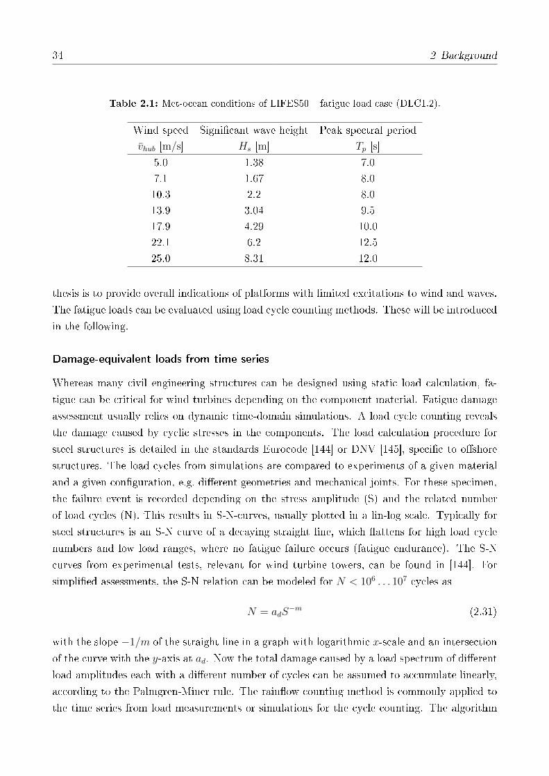
34 2 Background
Table 2.1: Met-ocean conditions of LIFES50+ fatigue load case (DLC1.2).
Wind speed Signicant wave height Peak spectral periodvhub [m/s] Hs [m] Tp [s]
5.0 1.38 7.07.1 1.67 8.010.3 2.2 8.013.9 3.04 9.517.9 4.29 10.022.1 6.2 12.525.0 8.31 12.0
thesis is to provide overall indications of platforms with limited excitations to wind and waves.
The fatigue loads can be evaluated using load cycle counting methods. These will be introduced
in the following.
Damage-equivalent loads from time series
Whereas many civil engineering structures can be designed using static load calculation, fa-
tigue can be critical for wind turbines depending on the component material. Fatigue damage
assessment usually relies on dynamic time-domain simulations. A load cycle counting reveals
the damage caused by cyclic stresses in the components. The load calculation procedure for
steel structures is detailed in the standards Eurocode [144] or DNV [145], specic to oshore
structures. The load cycles from simulations are compared to experiments of a given material
and a given conguration, e.g. dierent geometries and mechanical joints. For these specimen,
the failure event is recorded depending on the stress amplitude (S) and the related number
of load cycles (N). This results in S-N-curves, usually plotted in a lin-log scale. Typically for
steel structures is an S-N curve of a decaying straight line, which attens for high load cycle
numbers and low load ranges, where no fatigue failure occurs (fatigue endurance). The S-N
curves from experimental tests, relevant for wind turbine towers, can be found in [144]. For
simplied assessments, the S-N relation can be modeled for N < 106 . . . 107 cycles as
N = adS−m (2.31)
with the slope −1/m of the straight line in a graph with logarithmic x-scale and an intersection
of the curve with the y-axis at ad. Now the total damage caused by a load spectrum of dierent
load amplitudes each with a dierent number of cycles can be assumed to accumulate linearly,
according to the Palmgren-Miner rule. The rainow counting method is commonly applied to
the time series from load measurements or simulations for the cycle counting. The algorithm

2.7 Environmental Conditions and Load Calculation 35
used here is the one by Adam Nieslony4. The result is a histogram of the number of cycles njfor a given load range Sj. The total damage D is according to [146, p. 114] the sum of the
individual damage of each load range bin with nj cycles divided by the corresponding cycle
number Nj causing failure
D =k∑
j=1
njNj
=1
ad
k∑
j=1
nj (Sj)m ≤ η. (2.32)
Here, the simplied S-N curve model of Eq. (2.31) is used. Failure occurs when D exceeds the
usage factor η, depending on the component, see [146]. Fatigue is only assessed qualitatively
in this work as structural design calculations are outside the scope of this thesis. Therefore, a
reduced parameter representing the fatigue damage from a given load spectrum is used. It is
the load amplitude (usually a section force or moment), exerted during a hypothetical number
of cycles (here Nr = 2× 10⁶) giving the same D as the full load spectrum. The Damage-
Equivalent Load (DEL), represented by ∆Seq, can be calculated as
∆Seq,i = m
√1
Nr
∑
j
∆Smj nij. (2.33)
A weighting using a distribution function such as the one of Figure 2.6 is possible by multiplying
the load range number nij of the respective load range bin j with the lifetime fraction Ti/Tlifeof wind bin i giving
nij = njTiTlife
. (2.34)
In this simplied fatigue assessment, the inuence of the mean stress and stress amplication
factors due to the component geometry are not considered. Stress amplication at notches
is neglected and, as a consequence, the uniaxial stress is proportional to the section force, or
moment, see Section 3.2 for more details.
Damage-equivalent loads from frequency-domain spectra
The damage estimation from a given load spectrum with Eq. (2.32) requires load time series
from measurements or time-domain simulations to get the histogram with the cycle numbers njthrough a rainow counting algorithm. Various attempts have been made to obtain an estima-
tion of the load histogram from a frequency-spectrum. This has the advantage of a reduced
simulation time through frequency-domain methods as introduced in Section 2.6 and was es-
pecially necessary for the design of oshore oil and gas structures under stochastic loading
before computational power became aordable. A comparison of the dierent approaches can
4http://de.mathworks.com/matlabcentral/fileexchange/3026-rainflow-counting-algorithm, ac-cessed on January 22, 2018.

36 2 Background
be found in [147]. The most accepted method is the one from Dirlik [45]. It approximates the
number of cycles N for the dierent load ranges S. The Dirlik formula is written as
nj = E[P ] p(Sj)T, (2.35)
where E[P ] is the expected value of the number of peaks, a function of the second and fourth
spectral moments. The parameter p(S) is a nonlinear function of the zeroth, rst, second and
fourth spectral moments, see [147, Eq. 6]. The resulting number of cycles for each stress range
bin nj is given for a time period T . In order to obtain a representative set of cycle numbers
for each load range bin, the method of inverse transform sampling can be applied: From the
load range histogram nj a Cumulated Distribution Function (CDF) can be calculated through
an integration of the histogram over the bins of the load cycle numbers. The representative
set of samples (equal to the result of a rainow counting) can be obtained by assuming equally
distributed cycle counts, which are then mapped through the CDF from the count running sum
on the load ranges. The method has been implemented in the linearized model of Chapter 3
and compared to the conventional rainow counting method, see Section 3.9.
For the assessment of the controller, additional signals are of relevance, apart from the
structural loads. These are summarized together with the selected constraints for this work
in Table 2.2. The constraints on the left may not be exceeded, whereas the targets, usually
the signal Standard Deviation (STD) is sought to be minimized for optimal performance. The
indicated overshoots are evaluated in this work for one-hour time series. This is a simplication
for a straightforward quantitative design assessment, while for detailed design the probability
for a signal to exceed its bounds with respect to its lifetime needs to be calculated. The main
loads to be minimized by design and controller optimization are the tower-base loads. These
loads are the highest of FOWTs, compared to onshore turbines, see Section 2.5. Furthermore,
they represent the response of the tower-top displacement and also of the platform pitch motion.
These are important signals when looking at the overall FOWT system dynamics as already
discussed in Section 2.5.
Table 2.2: Requirements on controller performance.
Requirement Target
Rotor speed overshoot max. 15 % STD rotor speed min.El. power overshoot max. 15 % STD el. power min.Generator torque overshoot max. 15 % STD generator torque min.
STD blade pitch angle min.
2.8 Model Tests 37
Estimation of short-term extremes from frequency-domain spectra
A means to obtain short-term extreme responses from frequency-domain spectra will be in-
troduced in this section. This is especially useful for controller tuning when it is necessary to
get an estimate of the overshoot of the electrical power or the generator torque, the design
requirements shown in Table 2.2.
Assuming stationary Gaussian waves and a narrow-banded response signal, the response
amplitudes are Rayleigh distributed [90]. The short-term probability density function fst of the
amplitudes y is then given by
fst(y) =y
m0y
exp
(− y2
2m0y
). (2.36)
The zeroth spectral moment m0y of the response is equal to σ2y, the squared STD.
The probability of exceedance of the amplitudes y for a given time T can now be estimated
with the CDF Pst or the integral over the amplitude range of Eq. (2.36) as
Pst(y > a) =
∫ ∞
a
y
m0y
exp
(− y2
2m0y
)dy. (2.37)
The total number of occurrences NT of the values of y exceeding a limit a can be estimated
from the average zero-upcrossing period T2r. This follows from the conception that there is
only one peak value between an upcrossing and a subsequent downcrossing of any level a [148,
p. 237]. It results
NT =T
T2r
Pst(y > a). (2.38)
The amplitude which is reached or exceeded NT times in a given time T can be calculated
with Eq. (2.38), solving for the amplitude a. A comparison of this estimation with time-domain
data is also shown in Section 3.9, see Figure 3.29.
2.8 Model Tests
Experimental testing has become especially important for FOWTs due to the additional dy-
namics from the oating substructure, mooring lines and wave forces. Thus, model tests have
the objective to validate software tools in general, but as the TRL increases with the rst
tests in a realistic environment, model tests also helped to reduce the risk associated with the
deployment of a prototype.
It is common to the scaled testing of oshore structures to maintain a constant Froude
number Fr , see e.g. [91]. The Froude number is written with the characteristic length D, the
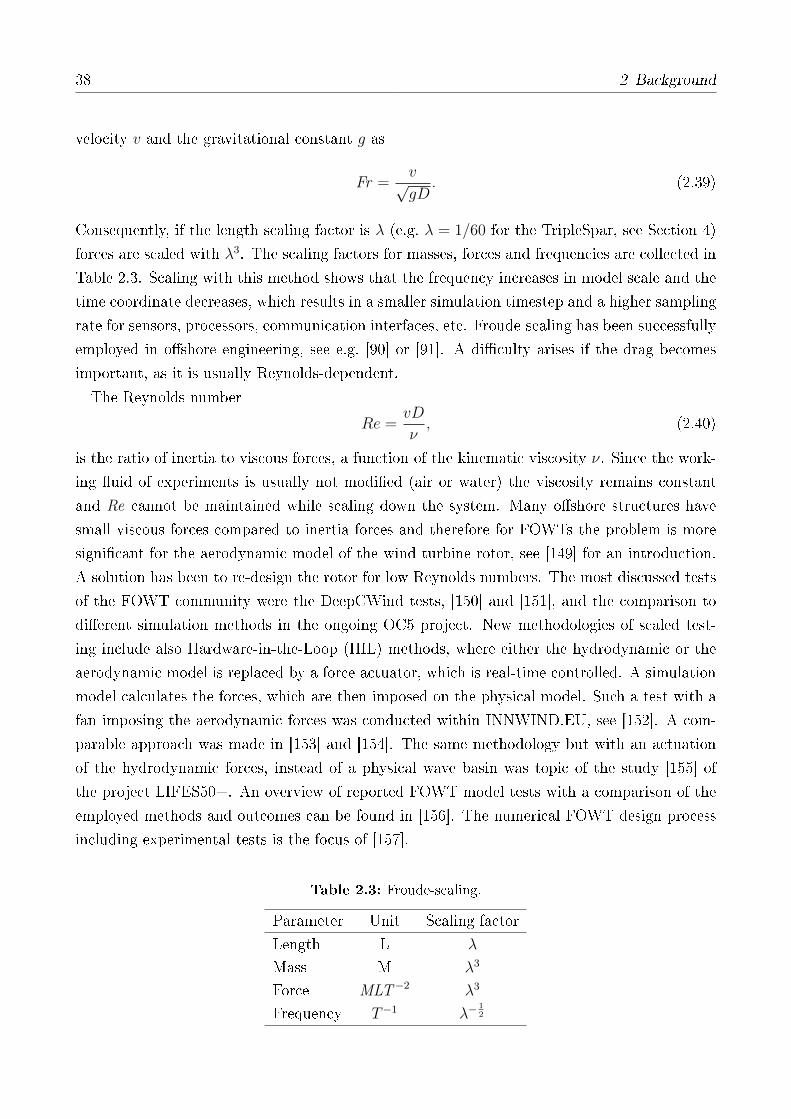
38 2 Background
velocity v and the gravitational constant g as
Fr =v√gD
. (2.39)
Consequently, if the length scaling factor is λ (e.g. λ = 1/60 for the TripleSpar, see Section 4)
forces are scaled with λ3. The scaling factors for masses, forces and frequencies are collected in
Table 2.3. Scaling with this method shows that the frequency increases in model scale and the
time coordinate decreases, which results in a smaller simulation timestep and a higher sampling
rate for sensors, processors, communication interfaces, etc. Froude-scaling has been successfully
employed in oshore engineering, see e.g. [90] or [91]. A diculty arises if the drag becomes
important, as it is usually Reynolds-dependent.
The Reynolds number
Re =vD
ν, (2.40)
is the ratio of inertia to viscous forces, a function of the kinematic viscosity ν. Since the work-
ing uid of experiments is usually not modied (air or water) the viscosity remains constant
and Re cannot be maintained while scaling down the system. Many oshore structures have
small viscous forces compared to inertia forces and therefore for FOWTs the problem is more
signicant for the aerodynamic model of the wind turbine rotor, see [149] for an introduction.
A solution has been to re-design the rotor for low Reynolds numbers. The most discussed tests
of the FOWT community were the DeepCWind tests, [150] and [151], and the comparison to
dierent simulation methods in the ongoing OC5 project. New methodologies of scaled test-
ing include also Hardware-in-the-Loop (HIL) methods, where either the hydrodynamic or the
aerodynamic model is replaced by a force actuator, which is real-time controlled. A simulation
model calculates the forces, which are then imposed on the physical model. Such a test with a
fan imposing the aerodynamic forces was conducted within INNWIND.EU, see [152]. A com-
parable approach was made in [153] and [154]. The same methodology but with an actuation
of the hydrodynamic forces, instead of a physical wave basin was topic of the study [155] of
the project LIFES50+. An overview of reported FOWT model tests with a comparison of the
employed methods and outcomes can be found in [156]. The numerical FOWT design process
including experimental tests is the focus of [157].
Table 2.3: Froude-scaling.
Parameter Unit Scaling factor
Length L λ
Mass M λ3
Force MLT−2 λ3
Frequency T−1 λ−12

2.9 Control 39
In the course of this research, two model tests were performed. One at the Research
Laboratory in Hydrodynamics, Energetics & Atmospheric Environment, Nantes, France
(LHEEA) in 2014 with the DeepCwind semi-submersible as part of the project INNWIND.EU5,
see [158, 159]. The other one focused on active blade pitch control on the TripleSpar semi-
submersible concept designed as part of this research and described in Section 2.10 with a
scaled 10 MW turbine, see [160]. This test was performed in a joint eort with DTU and Na-
tional Renewable Energy Centre of Spain (CENER). The experience from both tests was fed
back into the development of the reduced-order model of this thesis and a rst validation study
was done by Wei Yu in her thesis, see [161]. The hydrodynamic drag model of the simplied
simulation model of Chapter 3 will be validated through these tests and the drag coecients
of the TripleSpar platform will be identied in Chapter 4.
2.9 Control
This section provides the basics of modern wind turbine control and a review of challenges and
state-of-the-art control design methods for FOWTs.
2.9.1 Variable speed blade-pitch-to-feather-controlled turbines
The control system of modern wind turbines includes supervisory control for special events
like start-up and shut-down. The safety system regulates emergency shut-down events when
failures are detected to prevent damage to the turbine. Feedback control is mainly responsible
for capturing the maximum amount of energy from the wind through controlling the rotor speed,
depending on the wind conditions. In this work, the focus is on the feedback control of the
rotor speed. Feedforward control is benecial when information of the incoming disturbance
is known, such as wind and waves for wind turbines, see [162]. Feedforward control is not
considered in the present work.
The feedback control of wind turbines depends on the operating point with three regions and
the switchings in between. Region 1 covers wind speeds not relevant for energy production.
In region 2, the rotor speed is controlled by actuating the generator torque in a way that the
optimal TSR is maintained in order to capture the maximum amount of energy. Region 3 is
the above-rated region, where the blade pitch angle is actuated to control the rotor speed at
its rated speed and consequently maintaining the rated power. Earlier control methodologies
make use of the stall eect to reduce the lift force. This method avoids the blade pitch actuator
but is not present anymore in most modern wind turbines. An introduction to wind turbine
control can be found in [44] and [163].
5http://www.innwind.eu/, accessed on January 22, 2018.

40 2 Background
2.9.2 Floating wind turbines
Whereas below-rated control does usually not imply challenges for the design of FOWT con-
trollers, the coupled dynamics of the oating system pose diculties together with the blade-
pitch controller for above-rated wind speeds. A standard rotor-speed controller for above-
rated wind will pitch the blades when the rotor speed exceeds its rated value. In the case
of FOWTs, this feedback loop can imply, as a side-eect, that the tower or the platform ex-
periences large excursions. This is due to the aerodynamic properties of the rotor: When the
relative wind speed (the one seen by the rotor) increases, the controller will pitch the blades to-
wards feather (increasing blade pitch angle) and thereby reduce the aerodynamic rotor torque.
As a consequence, the thrust also decreases. This means, on the other hand, that an oscilla-
tion of the platform in pitch (about y, Figure 3.1) will become unstable if the controller reacts
suciently fast to the sinusoidally oscillating relative wind speed.
The contradicting goals of stabilizing power for above-rated wind speeds and minimizing
platform motion are a key challenge for FOWTs and of general importance for the fatigue
life, see [164]. A too aggressively tuned blade-pitch controller results in unstable platform
behavior. This is due to a Non-Minimum Phase Zero or Right Half-Plane Zero (RHPZ) of
oating platforms. This leads to a bandwidth reduction of the blade pitch controller. A good
explanation of this negative damping problem is given in [165]. A simple pole-placement
method to adjust the Proportional-Integral (PI)-controller to mitigate this negative damping
problem was proposed by [10]: The de-coupled rotor (including drivetrain) is considered as
rigid body in the closed loop (with active blade pitch control). Then the rotor closed-loop
eigenfrequency has to be selected lower than the critical support structure eigenfrequency,
which is usually the platform pitch frequency. This is roughly aligned with the general control
rule of thumb to limit the bandwidth for systems with RHPZs to half the frequency of the RHPZ
according to [166, p. 187]. The advantage of this procedure is that no linearized model of the
complete FOWT system is necessary but only the isolated rotor model and a quick denition
of reasonable control gains for conceptual design is rather straightforward. The disadvantage is
that rst, the isolated rotor eigenfrequency might deviate from the coupled rotor eigenfrequency
and therefore also the desired pole will deviate from the real pole of the coupled system. Second,
the overall system stability is not ensured with this method and therefore, instabilities might
still exist for certain operating points. The method was applied in [15] and compared with an
additional tower-feedback controller in [11] for a barge-type platform. An evaluation of this
method, also called de-tuning of gains was carried out by [167] and [168]. The comparison
in [169] includes also controllers with more than one feedback loop, in order to further improve
the control performance.
More advanced strategies are, among others, Multi-Input-Multi-Output (MIMO) controllers:
Here, the feedback of additional signals, the addition of more loops to the control architecture,

2.9 Control 41
can help to reduce the coupling eects in the system. The feedback of, e.g. the tower-top
acceleration is possible such that the blade pitch angle reacts not only to the rotor-speed
deviation but also to the tower-top acceleration. A sequential, manual tuning of feedback loops
and their respective gains, comparable to decentralized control, has been called multi-SISO
control, see [3, Appendix]. Real MIMO control looks at the FOWT system as a dynamic system
with multiple inputs (actuators like generator torque and blade pitch angle) and outputs (rotor
speed, tower-top displacement, etc.). As several standard linear control design methods do not
hold anymore for MIMO systems, the design process is more complex, see [170] for a study
on onshore turbines. Therefore, the authors of [12] published a parallel path modication
approach to mitigate the constraints from the RHPZ through the feedback of the tower-top
acceleration on the generator torque an approach published in the early stages of MIMO
control research, see [171].
Furthermore, optimal control design approaches have been presented, where optimization al-
gorithms are applied to nd the best feedback law, mostly using a linearized system description.
Such optimal controllers are a Linear Quadratic Regulator (LQR), as presented in [172], with
a state-feedback law. The LQR problem was extended to include nonlinearities of the FOWT
system in [173]. The optimal control problem in the frequency-domain can be solved with H2
or H∞ controllers, see [166]. Here, a target response (sensitivity function) is dened in the
frequency-domain with a given set of available sensors. This has been applied to onshore wind
turbines in [174, 175] and to FOWTs in [14] and [176]. Other multivariable controllers were
developed by [177], mostly using all or the most relevant system states as controller input. A
model development and Linear Model-Predictive Control (MPC) design can be found in [106]
and, especially aiming at wave disturbance preview in [178]. A comparison of dierent ap-
proaches for model predictive control for wind turbines can be found in [179]. An advanced
controller addressing specically the purpose of reducing disturbances is Disturbance Accomo-
dating Controller (DAC): A waveform of the disturbance is assumed and augmented to the
system as a feedforward term to cancel out the disturbance forcing. This was applied by [180]
and [181] to onshore wind turbines and to FOWTs in the thesis [182], among others.
Additional actuators to stabilize the tower were implemented in [105]. As was noted by [183],
the standard actuators of a turbine (generator torque and blade pitch angle) might not be strong
enough to mitigate rst-order wave loads. Here, additional actuators can help to improve the
motion response of a FOWT. For onshore turbines, passive systems like TMDs or tuned liquid
column dampers have been investigated. Also active systems are possible, see e.g. [105] and
the Master's thesis [184]. An additional actuator on the nacelle of a FOWT was proposed
by [185], an active vane to damp tower-top vibrations. A semi-active liquid column damper
with an optimal control approach was presented in [186]. In the project MARINA-platform,
the combination of a FOWT and a wave-energy converter was investigated and the potential to
produce energy from the waves. Possible approaches for such multipurpose oshore structures

42 2 Background
are compiled in [187]. For xed-bottom foundations structural damping devices have been
analyzed to reduce structural loads for large oshore wind turbines in [188], especially focusing
on the adaptation of the control to the actual structural properties. A general report on
methods for the mitigation of tower loads can be found in [189]. For oshore wind turbines,
various control approaches including tower feedback control were compared and assessed in the
thesis by Fischer [190]. Within the project INNWIND.EU dierent members and cross-braces
with specic dynamic properties are placed inside the tower or foundation to optimize the load
response something which is in general also feasible for FOWTs. Especially for damping the
blade response and smoothen the electrical power, smart blades, e.g. with aps, are subject to
research, see e.g. [191]. Many of these studies show that additional actuators oer the prospect
of damping the structural response with more or less use of actuator power. Some of these
systems are already being applied, i.e. TMDs in civil engineering, whereas others, like vanes
are still being analyzed in research projects.
With Individual Pitch Control (IPC), the blade pitch angles are not controlled simultane-
ously, as in the case of Collective Pitch Control (CPC), but individually. Thus, azimuth-
dependent forcing is possible, especially for reducing the 1p blade loads and the Three-Times-
Per-Revolution (3p) tower loads due to the vertical wind prole, see Section 2.7.1. A basic IPC
controller for wind turbines was proposed by Bossanyi in [192]. For FOWTs an extensive study
on IPC for FOWTs can be found in the thesis by Namik [182]. A FOWT controller for all
operational regions combining the prospects of DAC and Nonlinear Model-Predictive Control
(NMPC) with IPC is presented in [193] with a good improvement in terms of load reduction
compared to a standard controller but only short description of the modeling assumptions is
given.
Special approaches to improve the control performance for FOWTs were presented: In [194]
a set point change of the rotor speed as function of the platform pitch velocity was proposed.
This might be comparable to feedforward control such that the knowledge of the change in
relative wind speed at the rotor is used to determine the feedforward gain. Another proposed
approach is to use an estimator in real-time to distinguish the origin of the rotor speed deviation:
Whether it results from a forcing of waves on the support structure or from a change in the wind
eld. With an estimator it is possible to have the controller react primarily on the eects from
the wind eld uctuation and not the platform oscillation and thereby overcome the RHPZ
limitations. Additional sensors, mainly for disturbance preview for FOWTs, have been studied
with promising results: A feedforward controller using wind preview information on a FOWT
was shown in [108] and [195]. Light Detection And Ranging (LiDAR) signal data, used for an
advanced NMPC is presented in [106] and extended for IPC in [196].
First scaled experimental tests of FOWTs including active control were performed in [197]
in order to validate simulation models and assess the robustness of the control. Experimental
testing of FOWTs including control will be topic of Chapter 4 of this thesis.
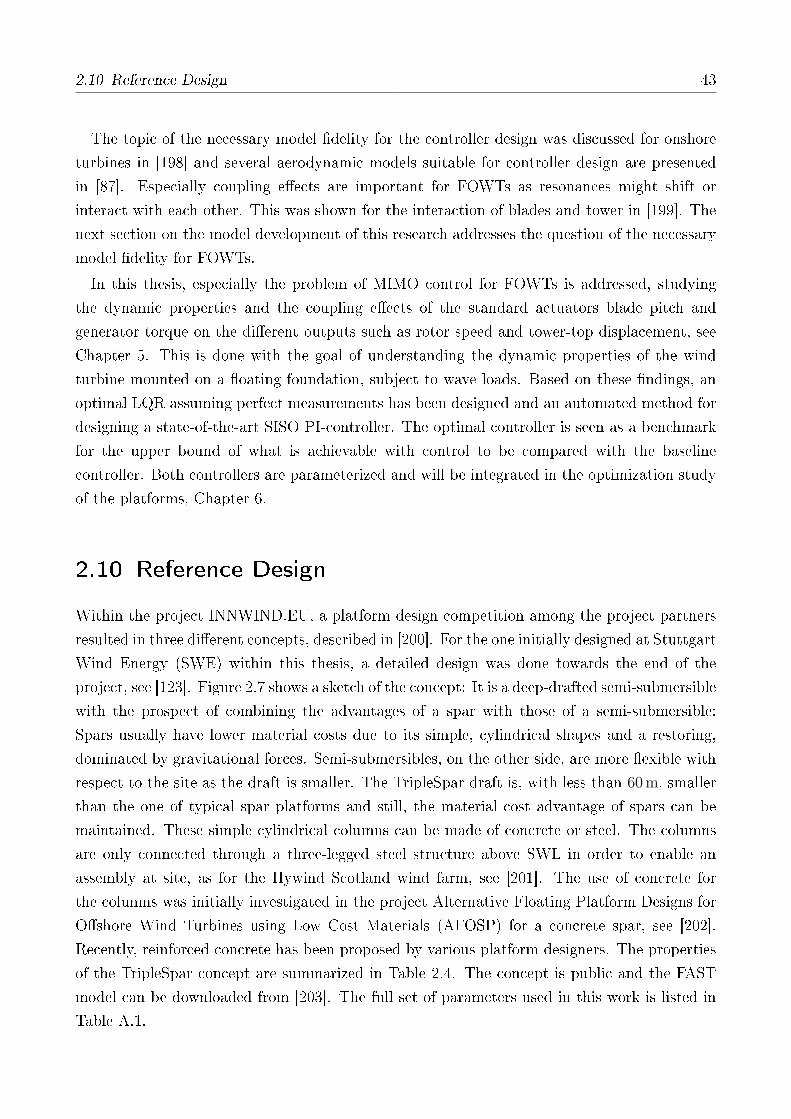
2.10 Reference Design 43
The topic of the necessary model delity for the controller design was discussed for onshore
turbines in [198] and several aerodynamic models suitable for controller design are presented
in [87]. Especially coupling eects are important for FOWTs as resonances might shift or
interact with each other. This was shown for the interaction of blades and tower in [199]. The
next section on the model development of this research addresses the question of the necessary
model delity for FOWTs.
In this thesis, especially the problem of MIMO control for FOWTs is addressed, studying
the dynamic properties and the coupling eects of the standard actuators blade pitch and
generator torque on the dierent outputs such as rotor speed and tower-top displacement, see
Chapter 5. This is done with the goal of understanding the dynamic properties of the wind
turbine mounted on a oating foundation, subject to wave loads. Based on these ndings, an
optimal LQR assuming perfect measurements has been designed and an automated method for
designing a state-of-the-art SISO PI-controller. The optimal controller is seen as a benchmark
for the upper bound of what is achievable with control to be compared with the baseline
controller. Both controllers are parameterized and will be integrated in the optimization study
of the platforms, Chapter 6.
2.10 Reference Design
Within the project INNWIND.EU, a platform design competition among the project partners
resulted in three dierent concepts, described in [200]. For the one initially designed at Stuttgart
Wind Energy (SWE) within this thesis, a detailed design was done towards the end of the
project, see [123]. Figure 2.7 shows a sketch of the concept: It is a deep-drafted semi-submersible
with the prospect of combining the advantages of a spar with those of a semi-submersible:
Spars usually have lower material costs due to its simple, cylindrical shapes and a restoring,
dominated by gravitational forces. Semi-submersibles, on the other side, are more exible with
respect to the site as the draft is smaller. The TripleSpar draft is, with less than 60 m, smaller
than the one of typical spar platforms and still, the material cost advantage of spars can be
maintained. These simple cylindrical columns can be made of concrete or steel. The columns
are only connected through a three-legged steel structure above SWL in order to enable an
assembly at site, as for the Hywind Scotland wind farm, see [201]. The use of concrete for
the columns was initially investigated in the project Alternative Floating Platform Designs for
Oshore Wind Turbines using Low Cost Materials (AFOSP) for a concrete spar, see [202].
Recently, reinforced concrete has been proposed by various platform designers. The properties
of the TripleSpar concept are summarized in Table 2.4. The concept is public and the FAST
model can be downloaded from [203]. The full set of parameters used in this work is listed in
Table A.1.
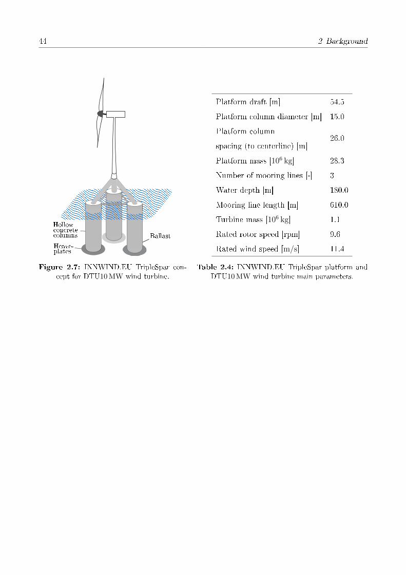
44 2 Background
Heave-
Ballastcolumns
Hollowconcrete
plates
Figure 2.7: INNWIND.EU TripleSpar con-cept for DTU10 MW wind turbine.
Platform draft [m] 54.5
Platform column diameter [m] 15.0
Platform column26.0
spacing (to centerline) [m]
Platform mass [106 kg] 28.3
Number of mooring lines [-] 3
Water depth [m] 180.0
Mooring line length [m] 610.0
Turbine mass [106 kg] 1.1
Rated rotor speed [rpm] 9.6
Rated wind speed [m/s] 11.4
Table 2.4: INNWIND.EU TripleSpar platform andDTU10 MW wind turbine main parameters.

3 Development of a Low-Order
Simulation Model
A tailored numerical model will be derived in this chapter, rst for a linear system analysis
and model-based control design and second, for a computationally ecient load calculation
and design optimization. A description of the model, together with exemplary results and
verication will be published in [204]. After the derivation of the structural model, all submodels
related to aerodynamics, hydrodynamics and the mooring lines will be described. The derivation
is shown for a nonlinear time-domain formulation with a linearization of each submodel. A
verication of the model, called Simplied Low-Order Wind turbine (SLOW) in the remainder,
through a comparison with FAST [43] will terminate the chapter. The next section will list the
functional requirements of the model with respect to its applications.
3.1 Requirements
State-of-the-art simulation models for FOWTs as introduced in Section 2.5 are engineering
models, which can be handled on standard PCs. Nonetheless, the computational eciency is
usually not high enough for large parameter variations in preliminary design stages.
Here, a list of requirements is formulated, for a simulation model enabling the goals specied
in Section 1.1. Full system optimizations shall be possible at early design stages with a reduced
simulation time to bridge the gap between simple spreadsheet calculations and DLC simulations:
• Fidelity: Representation of overall system dynamics, no resolution of components
• Speed: High computational eciency
• Functionality:
Suitability for model-based controller design and DLC-simulations
Nonlinear and linearized equations of motion
Only scalar disturbance inputs
• Architecture:
Fully parameterized
Flexible denition of Multibody System (MBS)
Portability among dierent platforms (symbolic Equation of Motion (EQM))

46 3 Development of a Low-Order Simulation Model
Based on these requirements, a model will be developed with dynamic equations derived from
physics rather than through system identication approaches using a more advanced model. For
a reduction of the computational time and code portability, the EQM are set up symbolically.
This means that the right-hand side of the ODE is not set up step by step with numeric values
but is available in the program code directly in terms of symbolic variables.
3.2 Structural Model
This section introduces MBS theory applied to the FOWT system with the goal of deriving EQM
with a reduced number of DoFs rst, for models of rigid bodies, linked by spring-damper
elements and then adding the theory of exible bodies for beam structures. Although the
derivation is conducted for a FOWT system, the description and also the code is set up in a
way that it is possible to simulate other mechanical systems as well. This diers from many
other MBS models in wind energy, which are exclusively set up for modeling HAWTs.
MSL
z
x
Ω
θ
βp
v0
yxp
xt
η
zp
Figure 3.1: Topology of the simplied multibody model (independent of oating platform con-cept), [205].
AMBS model is based on the assumption of a large rigid-body reference motion together with
small elastic deformations. This holds especially for rotating systems, such as any kind of tur-
bines. Wind turbines are especially challenging to model due to the exible tower and the highly
exible blades of ever increasing size. If no exible bodies are involved the rigid-body MBS
consists of point-mass bodies coupled with spring-damper elements. Newton's second law for
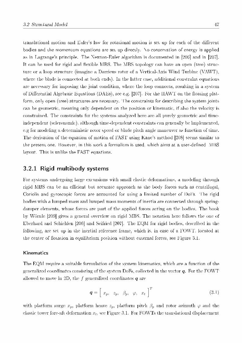
3.2 Structural Model 47
translational motion and Euler's law for rotational motion is set up for each of the dierent
bodies and the momentum equations are set up directly. No conservation of energy is applied
as in Lagrange's principle. The Newton-Euler algorithm is documented in [206] and in [207].
It can be used for rigid and exible MBS. The MBS topology can have an open (tree) struc-
ture or a loop structure (imagine a Darrieus rotor of a Vertical-Axis Wind Turbine (VAWT),
where the blade is connected at both ends). In the latter case, additional constraint equations
are necessary for imposing the joint condition, where the loop connects, resulting in a system
of Dierential Algebraic Equations (DAEs), see e.g. [207]. For the HAWT on the oating plat-
form, only open (tree) structures are necessary. The constraints for describing the system joints
can be geometric, meaning only dependent on the position or kinematic, if also the velocity is
constrained. The constraints for the systems analyzed here are all purely geometric and time-
independent (scleronomic), although time-dependent constraints can generally be implemented,
e.g for modeling a deterministic rotor speed or blade pitch angle maneuver as function of time.
The derivation of the equation of motion of FAST using Kane's method [208] seems similar to
the present one. However, in this work a formalism is used, which aims at a user-dened MBS
layout. This is unlike the FAST equations.
3.2.1 Rigid multibody systems
For systems undergoing large excursions with small elastic deformations, a modeling through
rigid MBS can be an ecient but accurate approach as the body forces such as centrifugal,
Coriolis and gyroscopic forces are accounted for using a limited number of DoFs. The rigid
bodies with a lumped mass and lumped mass moments of inertia are connected through spring-
damper elements, whose forces are part of the applied forces acting on the bodies. The book
by Wörnle [209] gives a general overview on rigid MBS. The notation here follows the one of
Eberhard and Schiehlen [206] and Seifried [207]. The EQM for rigid bodies, described in the
following, are set up in the inertial reference frame, which is, in case of a FOWT, located at
the center of otation in equilibrium position without external forces, see Figure 3.1.
Kinematics
The EQM require a suitable formulation of the system kinematics, which are a function of the
generalized coordinates consisting of the system DoFs, collected in the vector q. For the FOWT
allowed to move in 2D, the f generalized coordinates q are
q =[xp, zp, βp, ϕ, xt
]T(3.1)
with platform surge xp, platform heave zp, platform pitch βp and rotor azimuth ϕ and the
elastic tower fore-aft deformation xt, see Figure 3.1. For FOWTs the translational displacement

48 3 Development of a Low-Order Simulation Model
coordinates of the oating platform xp and yp are i.e. usually dened at the center of otation
of the platform and not at its Center of Mass (CM) in the same way as the inertial coordinate
system as described above.
The kinematic quantities of the translational velocity vi and the translational acceleration aiof each body's CM in inertial coordinates can now be calculated from the position vectors ri to
each body's CM. The velocity vi results from the position vector ri, dierentiated with respect
to time, as
vi(q, q) = ri(q, q) =∂ri(q, q)
∂qq = J t ,i(q, q)q (3.2)
omitting the partial dierentiation with respect to time, since no time-dependent boundary
conditions exist (scleronomic system). One can see that the Jacobian matrix J t ,i transforms the
kinematics, described in the inertial coordinate system, into the space of minimal coordinates,
see [206]. The same will be done later with the global Newton-Euler equations. As a result,
the EQM are a set of ODEs with one scalar equation per generalized coordinate and constrained
directions are not anymore part of the EQM. This has the major advantage that no additional
constraint equations are necessary and the EQM are available as ODE instead of a set of Partial
Dierential Equations (PDEs).
The translational accelerations ai are
ai = vi(q, q) =∂vi(q, q)
∂qq +
∂vi(q, q)
∂qq = J t,i(q, q)q + vi(q, q) (3.3)
with the component vi, called the local velocity.
The rotational generalized coordinates are also called quasi-coordinates as they cannot be
dierentiated directly yielding the angular velocity vector ωi. The vector of rotation angles αiis connected to the rotation tensor S(q) according to the selected description of the rotation.
For a rotation in three dimensional space, various descriptions are possible [210]. With Kardan
and Euler angles, the rotation matrix describes a successive rotation about the instantaneous
axes of the coordinate system. Therefore, it is important to keep in mind that simulation
results showing an angle about one axis represent the rotation about a rotated axis, not a xed
one. In this work, Kardan angles are selected with the sequence XZY , which is of advantage
for the rotation of the oating platform as the largest rotational displacement is usually in
pitch-direction (about y) due to wind and wave forcing. Consequently, the Kardan angle βp is
approximately the one about y of the inertial frame I. The rotation tensor can be written as
S =
1 0 0
0 cos(α) − sin(α)
0 sin(α) cos(α)
cos(γ) − sin(γ) 0
sin(γ) cos(γ) 0
0 0 1
cos(β) 0 sin(β)
0 1 0
− sin(β) 0 cos(β)
. (3.4)
3.2 Structural Model 49
The angular velocity vector ω = [ ω1, ω2, ω3 ]T results from the rotation matrix according
to [206]
SST =
0 −ω3 ω2
ω3 0 −ω1
−ω2 ω1 0
= S (ω) , (3.5)
where the cross-product operator S replaces the cross product
λ× a = S (λ)a. (3.6)
Note that a linearization of Eq. (3.4) yields a transformation matrix Slin , which does not
preserve the vector magnitude as tr(Slin) 6= 1. Corrections are possible, such as the one used
in the reference model FAST [15]. No corrections are employed for the linearized model in this
work. With the sequence of rotation of Eq. (3.4), the angular velocity vector remains as
ωi =
α
0
0
+
1 0 0
0 cos(α) − sin(α)
0 sin(α) cos(α)
0
0
γ
+
+
1 0 0
0 cos(α) − sin(α)
0 sin(α) cos(α)
cos(γ) − sin(γ) 0
sin(γ) cos(γ) 0
0 0 1
0
β
0
. (3.7)
This angular velocity holds for the body i, rotated by Si such that its local coordinate sys-
tem iei = [ 1 1 1 ]T is transformed to its counterpart in the inertial coordinate system Iei
byIei = Si
iei (3.8)
In this chapter, all quantities are dened in the inertial frame Ie and the superscript is omitted
for simplicity. This description of the rotation is used for all bodies in the MBS of the FOWT in
this work. In rotational directions, the Jacobian matrix J r,i can be calculated from the angular
velocity vectors as
J r,i =∂ωi(q, q)
∂q. (3.9)
The rotational acceleration of body i is then
αi(q, q) = ωi(q, q) =∂ωi(q, q)
∂qq +
∂ωi(q, q)
∂qq = J r,i(q, q)q + αi(q, q). (3.10)
Again, with the vector of the local angular acceleration αi(q, q), following the notation of [206].
50 3 Development of a Low-Order Simulation Model
Kinetics
Applied forces have to be dened for each body in the inertial coordinate system in the same
way as the kinematics. Applied translational forces F ai and torques Lai of rigid MBS are any
type of external forces, like aerodynamic or hydrodynamic forces, gravitational forces and forces
from the MBS coupling elements, e.g. spring-dampers. These forces are, other than the reaction
forces, known a-priori and not only after solving the EQM. They are usually calculated in every
timestep by external force models, which will be described in the following sections. The bodies
of the FOWT having a signicant exibility or elasticity are the tower and the blades. In this
work, a exible MBS with exible tower was generally used, except for the scaled experiments
of Chapter 4, where a rigid MBS was more suitable. In this case, a translational spring-damper
element at the tower-top can be dened. The overall stiness can be calculated by integrating
the sectional stinesses assuming a static shape and an approximate modal damping, see [211,
p. 375]. With this approach one portion of the tower mass is attributed to the platform and
another to the tower-top (RNA). A recommendation given in [163, p. 294] is to attribute 25 %
of the tower mass to the tower-top. Note that for the tower elastic restoring stiness the forces
on the nacelle are F anac = F spring
nac = −F springtwr due to the principle actio = reactio.
The reaction forces F ri and torques Lri acting on joints are unknown. For the calculation of
the response, they do not have any inuence and can be eliminated with the transformation
into minimal coordinates as is done in the next section. A discussion on how to calculate these
reaction forces and sectional forces of exible bodies will be made in Section 3.2.6.
Newton-Euler equations
With the described kinematics and kinetics, the equations of motions can be written. For the
translational directions, Newton's second law remains for each body i as
miai = F ai + F r
i . (3.11)
with the acceleration ai given by Eq. (3.3). The mass matrices mi ∈ R(3×3) contain the
body masses mi on the diagonal. In the same way as for translational motion, the angular
momentum (Euler-) equations are set up. The mass moments of inertia I i of each body i
are needed in the inertial coordinate system. As they are usually known in the body frame,
a transformation with the rotation tensor Si is necessary to obtain I i. The Euler equation
becomes with the angular acceleration αi of Eq. (3.10) following [206]
I iαi + S (ωi) I iωi = Lai +Lri . (3.12)
The global Newton-Euler equations for a total of p rigid bodies can now be put together
3.2 Structural Model 51
resulting in a set of (2 · 3 · p) equations as
miJ t,i...
I iJ r,i...
q +
miJ t,iq...
I iJ r,iq + S (ωi) I iωi...
=
F ai
...
Lai...
+
F ri
...
Lri...
. (3.13)
Now the reaction forces F ri and torques Lri can be eliminated according to the principle of
d'Alembert by multiplying Eq. (3.13) with the global Jacobian matrix
J =[J t,1, . . . J t,p, J r,1, . . . J r,p
]T(3.14)
from the left. Since the reaction forces always point into the constrained directions, perpen-
dicular to the generalized coordinates q, they are eliminated with this operation. After the
transformation Eq. (3.13) takes the form
M(q)q + k(q, q) = p(q, q) (3.15)
with the mass matrix M ∈ R(f×f), the Coriolis, centrifugal and gyroscopic forces k ∈ R(f×1)
and the applied forces p ∈ R(f×1). For a convenient numerical solution, Eq. (3.15) can be
transformed into state space by solving for the second derivative of the generalized coordinates q
and dening the state vector x as
x =dxdt
=
=
q
M−1(p− k)
. (3.16)
With the state vector of Eq. (3.1), selected for this work, the rotor is considered a rigid disk
and the structural model does not contain any dependency on the azimuth angle ϕ. In this
case, the azimuth angle is not a state as it is not necessary for a complete description of the
system and can be deleted from x. It is noted that the closed-loop system includes ϕ as state
again when introducing an aerodynamic force model, which includes an azimuth-dependency
or a rotor speed controller with an integral term.
Added mass forces
For oating bodies, an acceleration-dependent force needs to be added to the inertia-term of
Eq. (3.13) in the same way as in the rigid-body EQM, Eq. (2.19). The added uid mass depends
on the hull shape and is usually calculated by potential ow (or panel-) codes. Depending on the
reference point and the symmetry, the added mass matrix A(ω) ∈ R(6×6) has coupling elements
52 3 Development of a Low-Order Simulation Model
between translational and rotational DoFs. These coupling terms need to be respected in
Eq. (3.13). In the present model this is solved by writing the structural mass matrices for all
bodies i as M i ∈ R(6×6) including the translational mass matrices and the mass moments of
inertia. From these, the left summands of Eq. (3.13) result from
miJ t,i
I iJ r,i
= M i
J t,iJ r,i
. (3.17)
For the planar (2D) EQM, the most important coupling terms are usually the surge-pitch (5,1)
and (1,5)-elements. This becomes even more important when the reference point for the added-
mass matrix is the CF (at the water surface, as is the usual procedure and also done in this work)
because this point is distant from the Center of Buoyancy (CB). The frequency-dependency
of A is further discussed in Section 3.5.1.
3.2.2 Flexible multibody systems
In this section, the EQM for rigid MBS will be extended to account also for exible (elastic)
bodies. The exible MBS approach simplies the inclusion of all body forces from large displace-
ments of the reference frame. These are dicult to obtain from standard FE approaches, which
require the computationally expensive absolute nodal coordinate formulation, see [210] for de-
tails, or hybrids like the co-rotational frame formulation implemented in 3DFloat, see [212]. A
derivation of a nonlinear FE model for wind turbines can be found in [213] for the tool FAST.
The notation here follows the one from Schwertassek and Wallrapp [59]. The assembly of the
equations, equivalent to the ones of rigid systems, Eq. (3.13), follows Seifried [207], because he
uses d'Alembert's principle, as opposed to [59], who use Jourdain's principle for the elimination
of the reaction forces. The vector of generalized coordinates q will be a combination of rigid
and exible (elastic) DoFs q = [qr, qe]T . With a exible tower, the vector q, dened for rigid
bodies in Eq. (3.1), is composed of a rigid and a exible part as
qr =[xp, zp, βp, ϕ, θ1
]Tand qe =
[xt
]. (3.18)
In Chapter 5 and 6, the collective blade pitch actuator is included in the exible MBS with
a single DoF θ1. The next sections describe the derivation of the additional equations to the
Newton-Euler equations of Eq. (3.13) to represent exible bodies. Therefore, the index i refers
to a exible body in this section.
3.2 Structural Model 53
Kinematics
The present derivation follows the oating frame of reference method, see [59] and [214]: It is a
reference coordinate system for the denition of the exible body, which is not necessarily its CM
but any reference point that is convenient for the description of the elastic properties. This
formulation simplies parts of the equations and is useful for a pre-computation of the elastic
properties of the bodies, which is detailed at the end of this section. Eventually, the kinematics
of an elastic body i can be described by the reference kinematics with a large nonlinear motion
and the small linear motion described by the fe,i generalized elastic coordinates qe,i ∈ R(fe,i×1)
of body i.
The coordinates (in the local body reference frame R) of the nodes k of a exible body in
the reference conguration (undeformed) with respect to the reference system are collected in
the vector R = RR. The deformation eld Ruki (t) of the body is dened in the local frame for
each node k relative to the reference coordinates RR. The position vector ρki (t) to the exible
nodes k, using the oating frame of reference is in the local reference frame R
Rρki (t) = Rri(t) + RRki + Ruki (t) = STi
Iρki (t). (3.19)
For the orientation the same description holds: In the same way as Rki , the tensor Γk
i represents
the orientation of node k of the exible body i in the reference conguration with respect to
the reference frame.
Looking at a straight rotor blade with the z-coordinate of ei pointing to the blade tip, the
beam reference coordinatesRi, aligned with the shear axis of the beam, see [60], will have zero x
and y-coordinates and the entries in x-direction are the radial position of the blade stations,
the same as in FAST [39]. For a pre-bent blade such as those of the DTU 10 MW RWT, this
is not the case and also the orientation of Γki is not constant for dierent k, due to the blade
twist and the pre-bending.
A deformed body has the nodal orientation
Dki = Θk
i (t)Γki (3.20)
with the additional rotation from the deformation dened by the rotation tensor Θki (t). The
rotation tensor Dki is dened in the same way as Si according to the convention of Eq. (3.8).
Shape functions As in FE models, shape functions are used to avoid having to solve the PDEs
of continuum mechanics. With the Ritz-approach, the time-dependent and space-dependent
solution can be separated: Time-independent characteristic shapes are used to approximate the
deformation and are integrated to the ODE to solve for a time-dependent response. For MBS,
this approach can also be used by approximating the deformation of a exible body with a

54 3 Development of a Low-Order Simulation Model
characteristic shape. This is part of MOR techniques, one of which is the Guyan reduction,
which uses static modes of the exible body as shape functions. In the present model, the
mode shapes of importance for the system dynamics will be used. For a recent work on MOR
methods in structural dynamics see [215] and specically to wind turbines [216].
The shape function for translation Φki ∈ R(3×fe,i) for each node k has fe columns, as many as
generalized elastic coordinates dened for exible body i. For the rotation, the shape function
is Ψki ∈ R(3×fe,i). Note that one shape function represents a translational and at the same time
rotational displacement. The nodal rotation tensor Θki (t) can be calculated from the rotation
shape function ϑki for small displacements with the identity matrix E as
Θki (t) = E + S
(ϑki). (3.21)
The general relative deformation eld for translation uki (t) of Eq. (3.19) and for rotation ϑki (t)
of Eq. (3.20) can now be written as function of the generalized coordinates of the elastic
body qe,i(t)
uki (t) = Φki qe,i(t) ϑki (t) = Ψk
i qe,i(t). (3.22)
For beam models, used in this work for the tower, the shape functions are written as function
of the beam axis x ≡ R1. Here, one mode shape is used to represent the tower elasticity in
fore-aft direction. The shapes for a linear Bernoulli beam with only one DoF for bending take
the form1
Φi(R) =
Wi,1(x)
0
−R2W′i,1(x)
, (3.23)
where Wi,1(x) stands for the lateral deection of the beam axis for the rst shape. The shape
function for the beam element rotations reads
Ψi(R) =
0
W ′i,1(x)
0
. (3.24)
Looking at Eq. (3.22), it becomes clear that the shape functions Φi(R) and Ψi(R) have more
than one column for qe,i containing more than one coordinate.
As a result, the overall orientation ISki with respect to the inertial coordinate system I of
1Here written as continuous function of R and not for the nodes k as the shape functions are usually approx-imated by analytic expressions.

3.2 Structural Model 55
node k can be calculated using Eqs. (3.21) and (3.22) as
Ski =(E + S
(Ψki qe,i(t)
))ΓkiSi(t), (3.25)
where the rotation of the reference system of body i is Sk=0i = Si. Equation (3.25) is of
importance for the denition of the orientation of a new body attached to a exible body, for
example the nacelle mounted at the tower-top. In that case, the end node k of the tower gives
the nacelle orientation Snac = Sktwr. In the same way the angular velocity ωki can be calculated
from the rotation tensor Ski using Eq. (3.5) or, as done in this model, from the denition of
Kardan angles, Eq. (3.7). The nodal velocities relative to the inertial frame I can be obtained
by dierentiating Eq. (3.19) with respect to time in either the reference or the inertial frame.
Eventually, the kinematic functions for velocity zII,i and acceleration zIII ,i can be expressed
using minimal coordinates with the Jacobian matrices J t,i and J r,i following [207] as
zII ,i =
Rvi
Rωi
qe,i
=
J t,i(q)
J r,i(q)
J e,i
q and zIII ,i =
Rai
Rαi
qe,i
=
J t,i(q)
J r,i(q)
J e,i
q +
J t,i(q, q)
J r,i(q, q)
0
q.
(3.26)
Consequently, the kinematics of elastic bodies are described by a reference translational and
rotational motion as for rigid bodies, see Eq. (3.2)(3.7), but additionally by the generalized
coordinates of the elastic motion qe,i. Thus, there are fe additional equations in the (2 · 3)
Newton-Euler equations (Eq. (3.13)) for each elastic body i. The selection matrix J e,i assigns
the elastic coordinates qe,i of q to the corresponding bodies and therefore these elastic equations
are unchanged when transforming the system into minimal coordinates. The global Jacobian
matrix J , dened for rigid bodies in Eq. (3.14), is for exible bodies
J =[J t,1, J r,1, J e,1, . . . J t,p, J r,p, J e,p
]T. (3.27)
In the case of elastic bodies, the kinematics are written in the reference coordinate system
denoted by the superscript R, taking advantage of the oating frame of reference approach
as introduced at the beginning of this section. The kinematics of the rigid bodies within the
global MBS of rigid and exible bodies, however, are still written in the inertial coordinate
system I as derived in Section 3.2.1.
Selection of the body reference frame The reference frame R for the elastic body does not
have to be the body-CM as for rigid bodies of Section 3.2.1. A guidance for the choice of the
location of the reference frame is given in [59, p. 257]. For the tower-body, the tower-base is

56 3 Development of a Low-Order Simulation Model
selected with the z-axis aligned with the beam axis. Thus,
u0i (t) = 0 and ϑ0
i (t) = 0. (3.28)
In this case also the shape functions Φki and Ψk
i need to obey this condition, i.e. for a beam
the derivative of the shape functions is with respect to the beam axis W ′(x= 0) = 0. For a
hinge joint at the reference frame of the exible body, the reference frame orientation depends
on the elastic generalized coordinates, qe,i. For a FOWT tower this can be the case due to
the oating foundation. It is possible to obtain the tower mode shapes including a exible
foundation with an unreleased version of the tool BModes [217] by NREL. This has not been
done in this work for simplicity. With the kinematics the body forces consisting of inertial,
gravitational, centrifugal, Coriolis, gyroscopic and elastic forces can be calculated.
Kinetics
The kinetics of elastic bodies dier from those of rigid bodies as the eects of the body de-
formation have to be included in the calculation of the body forces. The notation is dierent
from the one of rigid bodies, following the reference book for the model setup [59] (in German).
In the book by Shabana [214], the same derivation can be found in English, although with a
dierent notation and a description in the inertial frame instead of the body reference frame.
The Newton-Euler equation for an elastic body i includes the mass matrixM i, the quadratic
velocity vector hω,i with Coriolis, centrifugal and gyroscopic forces, gravitational forces hg,
applied discrete forces hd,i, inner elastic forces he,i, based on the selected deformation tensor
and again, the reaction forces hr,i
M izIII ,i + hω,i = hg,i + hd,i + he,i + hr,i. (3.29)
In the following the components of Eq. (3.29) will be derived. For simplicity, the index for the
body i will be omitted as all equations are set up initially for a single body.
Mass matrix The mass matrix for a exible body i for the generalized coordinates zI is
according to [59]
M =
M tt sym.
M rt M rr
M et M er M ee
=
m sym.
mS (c) I
Ct Cr M e
. (3.30)
One can see that the entries of M related to translations t, rotations r and elastic coordi-
nates e contain coupling elements. This means that inertial forces on the exible body frame R

3.2 Structural Model 57
result from a generalized acceleration qe and vice-versa. Couplings between translations and
rotations do not appear in the case of rigid bodies, Eq. (3.13), because for rigid bodies the
position vectors ri always point to the respective CM. The same happens when transforming
the rigid EQM from one reference point to another (meaning that the Newton's and Euler's law
are written with a reference point other than the body-CM) using the system transformation
matrix dened in [218, p. 176], see also Section 3.5.3.
The CM c of the exible body can be obtained for beams with cross-section A, length l and
density ρ through an integration along the beam axis x as
c =1
mi
∫ l
0
ρAxdx+1
mi
CTt qe. (3.31)
The second summand, Ct ∈ R(fe×3), is the inuence from the body deformation
Ct =
∫ l
0
ρAΦTi (x)dx. (3.32)
The mass moment of inertia I = I(qe) is the sum of the one of the undeformed body I0 and
the contributions from elasticity I1(qe) and I2(qe)
I(qe) = I0 + I1(qe) + I2(qe) with (3.33)
I1 =
∫ l
0
(S (R) S (Φqe)
T + S (Φqe) S (R)T)dm and I2 =
∫ l
0
S (Φqe) S (Φqe)T dm.
The coupling between elasticity and rotations Cr is given by
Cr =
∫ l
0
ΦT S (Φqe)T dm. (3.34)
The mass matrix of the generalized elastic coordinateM e can be calculated by integrating over
the squared shape functions
M e =
∫ l
0
ΦΦTdm. (3.35)
Gravitational forces The gravitational body forces hg also depend on the deformation of the
body with the vector of the gravitational acceleration g = [ 0, 0, g ]T as
hg =
E
S (R+ Φqe)
ΦT
dm g =
m
mS (c)
Ct
g. (3.36)
58 3 Development of a Low-Order Simulation Model
Inner elastic forces The inner elastic forces give, integrated over the volume of the exible
body for each mode shape, the restoring stiness and structural damping forces on the MBS.
Thus, the strain can be calculated with the parameterized shape of deformation of the body.
From the strain the stresses can be computed with the material law. A number of transforma-
tions is necessary, depending on the coordinates used to parameterize the deformed shape as a
space curve. Here, a short overview is given for Bernoulli beams, which are used in this work.
The Green-Lagrange strain tensor reads in a linearized formulation for small displacements
following [59, p. 79]
Gij =1
2
(∂ui∂Rj
+∂uj∂Ri
)(3.37)
and gives the strain vector
ε = [ G11, G22, G33, 2G12, 2G23, 2G31 ]T . (3.38)
With this denition, the strains can be calculated from a given deformation. Often the defor-
mation is written in terms of the beam coordinates
ν(x, t) =[w1(x, t), w2(x, t), w3(x, t), ϑ1(x, t)
]T, (3.39)
where
w = Wqe. (3.40)
Thus,W = W ∈ R(3×fe) has the same dimension as the matrix of shape functions Φ, compare
Eq. (3.23). For Bernoulli beams deformed in 3D including torsion about the beam axis ϑ1, the
general displacement eld is given by [59, Eq. (4.86)] as
u =
w1 +R2 (−w′2 + w′1w′2 − ϑ1w
′3) +R3 (−w′3 + w′1w
′3 + ϑ1w
′2)
w2 −12R2 (w′22 + ϑ2
1) −R3 (ϑ1 + w′2w′3)
w3 R2ϑ1 −12R3 (w′23 + ϑ2
1)
. (3.41)
Applying now Eq. (3.37) on the displacement eld, Eq. (3.41), the strain for Bernoulli beams
results as
G11 = w′1 −R3w′′3 −R2w
′′2 ,
G12 = G21 = −1
2R3ϑ
′1, G13 = G31 =
1
2R2ϑ
′1, (3.42)
G22 = G33 = G32 = G23 = 0,
3.2 Structural Model 59
see [59, Eq. (6.423)]. For large reference motions, the assumption of small deections is often not
valid anymore. This is for example the case for a rotating blade on a wind turbine rotor, which
usually shows increasing blade eigenfrequencies with an increasing rotational speed through
centrifugal stiening. Here, quadratic terms are necessary, which can be included in a linearized
fashion in G, see [59, Eq. (6.424)].
The remaining part is a transformation of the strain tensor G, because the strain is needed
as function of the generalized elastic coordinates qe. With this end the matrix BL is introduced
ε = BLqe. (3.43)
Note that BL ∈ R(6×fe) contains only the linear terms. For the nonlinear terms BN , resulting
for example from geometric stiening (centrifugal stiening) refer to [59, p. 356]. Comparing
now the denition of the strain vector ε, using Eqs. (3.38), (3.42) and (3.43), one can derive BL
and consequently the strains ε as function of the generalized elastic coordinates qe. For a linear
Bernoulli beam without the DoFs for longitudinal extension and torsion, as implemented in
this model, all elements of the Green-Lagrange strain tensor G vanish except for G11 and the
linear restoring stiness for mode k = 1 can be calculated with the Young's modulus E as
KeL =
∫
V
BTLEBLdV =
∫ l
x=0
EJ22W′′21 (x)dx. (3.44)
The integration over the cross-section A with the lateral coordinate R1 yields the second mo-
ment of area J22 about y. The linear generalized stiness matrix KeL ∈ R(fe×fe) has as many
rows and columns as elastic degrees of freedom, dened for the body. Thus, the diagonal
entries are the modal stinesses, which can be also used as spring stiness when using the
rigid MBS of Eq. (3.13). For the tower, the rst mode can be used as dominant mode giv-
ing F atwr(1) = KeL,twr(1, 1)xt. Looking at Eq. (3.44), it becomes clear that the modal stiness
matrix, which determines the dynamics of the exible MBS, depends on the material, but clearly
on the shape function (with its second derivative W ′′, squared). Thus, a modied shape, i.e.
from dening a dierent tower-top mass in tools like BModes [217], will change the modal
stiness.
The structural modal damping matrix De ∈ R(fe×fe) can be calculated from the modal
stinessKeL and the modal massM e for mode k assuming a given structural damping ratio ξk
De = diag(Dek) with Dek = 2ξk√KekMek. (3.45)
Thus, for a constant structural damping ratio dierent modal damping ratios can be calculated,
depending on their corresponding modal stiness. The modal damping ratios are user-dened
inputs in FAST [43].
60 3 Development of a Low-Order Simulation Model
Finally, the vector of inner elastic forces he results as
he =
0
0
−KeLqe −Deqe
. (3.46)
External applied forces External forces in this FOWT model are the ones from aerodynamics
and hydrodynamics, subject of the next sections. In order to include them, they need to be
transformed into the space of the generalized coordinates representative for the exible bodies.
The discrete applied forces hd of Eq. (3.29) are again a combination of translational, rotational
and elastic forces, aligned with the generalized coordinates zII and zIII , dened in Eq. (3.26).
Based on the nodal forces F k and torques Lk in the reference frame the generalized forces are
hd =
hdt
hdr
hde
=
∑
k
E
S(Rk + Φkqe
)
ΦkT
F
k +
0
E
ΨkT
L
k
. (3.47)
Quadratic velocity vector The contributions from centrifugal, gyroscopic and Coriolis forces
are combined in the quadratic velocity vector hω of Eq. (3.29). As these forces are of minor
importance for the FOWT moving in 2D and no bodies are attached to the spinning rotor,
the derivation is omitted here and can be looked up in [59, p. 296] (for a reference in English
see [207]). Still, the quadratic velocity vector is implemented in the present model.
The global Newton-Euler equations of each, rigid and elastic, body are now complete and
can be transformed into minimal coordinates with the assembled global Jacobian matrix J for
rigid bodies of Eq. (3.14) and for exible bodies of Eq. (3.27) such that the nonlinear EQM
result in the form of Eq. (3.15).
Standard Input Data Many kinematics and kinetics functions can be written as function of
the generalized elastic coordinates qe,i. They can therefore be computed independently of the
response of the MBS. This is due to the description of the exible body in the body reference
frame R. A standard format was dened in [219] to provide an interface between FE models
calculating the elastic properties in a pre-processing step for the subsequent solution of the MBS
model. With this format, exible bodies can be pre-computed in FE tools and exported to be
used in MBS codes. The Standard Input Data (SID) format is object oriented and the arrays
are stored depending on the order of qe. Part of the SID are the reference coordinates R, the
shape functions, Φ and Ψ, the product mc, the elements of the mass matrix M , Eq. (3.30)
and the stiness and damping matrices Ke and De, respectively, among others. The SID is
calculated in the present model in a dedicated function for beam structures.

3.2 Structural Model 61
3.2.3 Additional dynamic couplings
Next to the MBS equations derived above, the FOWT includes several dynamic couplings,
which do not require a mechanical multibody model. The blade pitch actuator, for example,
is usually modeled as a time-delay or a second-order dynamic transfer function from the com-
manded blade pitch angle to the measured blade pitch angle. Another example is the drivetrain
exibility resulting in a dynamic coupling between the aerodynamic torque and the reaction
torque between the gearbox housing and nacelle. These dynamics can be written as user-dened
dynamics, setting up the right-hand-side of an ODE in the input le to the EQM.
In the present model, the rotor shaft exibility is neglected. This can be justied with the
controller bandwidth. All controllers used have a bandwidth below the tower eigenfrequency.
This reduces signicantly the external forcing at the torsional shaft eigenfrequency, which is
usually above the tower eigenfrequency. The blade pitch actuator is modeled as a second-order
transfer function with eigenfrequency and damping ratio given in Appendix A.
3.2.4 Symbolic programming
As main target of the SLOW model a high computational eciency was highlighted in Sec-
tion 3.1. In order to meet this goal and to allow for a high independence of the platform
and the programming language, the EQM of the structural model are written using symbolic
programming. As a result, the EQM are well portable and can be implemented on real-time
systems. However, when using symbolic programming, a number of limitations has to be kept
in mind: The size of the equations must not exceed a certain limit depending on the compiler
and the code optimization routines implemented in it. Especially multiple rotations in the tree
structure of the MBS increase the size of the equations and lead to long compilation times.
An assessment of the compilation times for symbolic codes can be found in [38]. On the other
side, the above derivations, specic to exible bodies as opposed to rigid bodies, do not di-
rectly lead to large equations and do not necessarily increase the computational time. A ow
chart with the tool architecture from the derivation of the EQM down to the time-domain and
frequency-domain results is shown in Section 3.7.
3.2.5 Linearization
The structural EQM are linearized symbolically by calculating the Jacobians with respect to
the states x of all variables of the global nonlinear EQM, Eq. (3.15), of rigid and exible bodies.
With system inputs (control and disturbance inputs) dened in vector u (e.g. rotor-eective
wind speed v0, blade pitch angle θ, etc.), the equations are linearized about the set point of the

62 3 Development of a Low-Order Simulation Model
states x0 and the setpoint of inputs u0
x = x0 + ∆x u = u0 + ∆u, (3.48)
where ∆x and ∆u are the new vectors of dierential states and inputs, respectively. For
all linear descriptions, ∆ will be omitted in the following for brevity. The coupled nonlinear
equations of motion in state-space description can be separated for position- and velocity-
dependent terms. It remains with the input matrix B
x =
0 E
−M−1Q −M−1P
︸ ︷︷ ︸A
x+Bu. (3.49)
One can identify the position-dependent matrix Q and the velocity-dependent matrix P , which
both result from the transformation of the vector of Coriolis, centrifugal and gyroscopic forces
and the applied forces. The linearization of the force model will be addressed together with
the description of the external force submodels in Section 3.33.6. The linearization is most
critical for the aerodynamic force coecients due to its highly nonlinear behavior.
3.2.6 Time-domain motion and load response signals
For structural design, especially the stresses inside the components are of interest to assess
static or dynamic integrity in ULS or FLS analyses as initially introduced in Section 2.7.3.
For controller design, also the position, velocity and acceleration of components are of interest,
in order to damp certain responses and make sure design limits are not exceeded. Therefore,
coordinate systems or nodes of exible bodies can be dened at locations other than the ones
where the generalized coordinates q are dened, or be expressed in other coordinate systems.
Often the absolute tower-top displacement, in inertial coordinates is needed and not the one
relative to the tower-base frame as the generalized coordinate xt.
Section forces or structural stresses can be calculated based on the generalized elastic co-
ordinates of exible bodies qe, see [59, p. 357]. The therein presented approximation of the
section forces is straightforward and can be easily implemented in computational algorithms.
It neglects, however the dynamic component, as it depends only on the position of the elastic
coordinate: Looking at bending only, as for the inner elastic force calculation in Eq. (3.44), the
information on the second derivative of the shape function W ′′l (x), related to the considered
elastic coordinate l, is necessary. The bending stress σb as function of the beam longitudinal
coordinate x and the lateral coordinate in the cross-section R1 is
σb(x,R1) = −ER1W′′l (x)qe,l. (3.50)
3.2 Structural Model 63
The approximation remains for the internal bending moment Lb(x)
Lb(x) = EJ22W′′l (x)qe,l. (3.51)
For a more exact calculation, considering also velocity-dependent sectional loads (including
inner elastic forces due to structural damping), the same approach is used here for rigid and
exible MBS. Assuming a modal spring-damper element at any longitudinal location along
the beam axis gives the section forces as the forces exerted by this spring-damper element. At
the tower-top, the sectional forces F tt are
RF tt =
−ktwrxtwr − dtwrxtwr0
0
, (3.52)
with the tower modal stiness ktwr and damping dtwr. These constants can be selected to
be equal to the dominant modal stiness and damping coecients within KeL and De of
Eq. (3.46). This force produces a sectional moment along the tower axis, which can be used to
calculate the stresses with the second moment of area J22 using the basic laws of mechanics.
3.2.7 Frequency-domain motion and load response spectra
From the linear state-space description of Eq. (3.49), SISO transfer functions from a specic
input to a specic output can be derived using Eq. (2.25). Applying frequency-domain spectral
methods the response spectra can be calculated without time integration. The response PSD
Syy(ω) results with the transfer function G(ω) and its complex conjugate transpose G(ω)∗T
and the disturbance spectrum Sdd as
Syy(ω) = G(ω)SddG(ω)∗T . (3.53)
Note that the FOWT plant model G(ω) includes the structural model and the disturbance
models, part of Section 3.33.6. In order to simplify the computation, the response spectra
from wind and waves (d = [v0, ζ0]T ) are calculated by assuming that the cross-spectral density
between wind and waves is zero Sdd(1, 2) = Sdd(2, 1) = 0. It results
Syy(ω) = Gv(ω)SvvG(ω)∗Tv +Gζ(ω)SζζG(ω)∗Tζ . (3.54)
Section forces
The section force calculation will be derived here in the frequency-domain with the rened
method of Eq. (3.52), including the velocity-dependent forces. The simplied method, neglect-
64 3 Development of a Low-Order Simulation Model
ing the velocity-dependent forces, does not always yield a good agreement with the reference
model FAST. Based on Eq. (3.52), the tower-base bending moment Myt can be calculated.
Additionally to the elastic forces, which depend on the tower DoFs, the pitch-DoF-dependent
forcing due to gravity needs to be included. The static transfer function
HMy =
cT0,z
KeLztt
Deztt
, HMy ∈ R(3×fe) (3.55)
is used to calculate the tower-base bending moment cross-spectral density matrix SMyMy . The
vector cT0,z of Eq. (3.36) represents the center of mass of the tower in tower-base coordinates
(tower reference frame). As the tower is modeled through a single mode shape, HMy is a
column vector here. The PSD of the tower-base bending moment results as
SMyMy(ω) = HMy(ω)Syy(ω)H∗TMy(ω). (3.56)
For the computation, the reduced response spectral density matrix Syy(ω) is used, which in-
cludes a reduced set of system outputs: The pitch (βp)-DoF and the tower-top states xt and xt.
Electrical power
The calculation of the electrical power P is a quadratic problem, it is the product of the
generator speed Ωg and the generator torqueMg. This is why it is especially addressed here for
the frequency-domain model. In the time-domain, the electrical power can be calculated with
the static components Mg0 and Ωg0 and the uctuating components ∆Mg and ∆Ωg with the
eciency of the generator ηgen as
P = ηgenMgΩg = ηgen(Mg0 + ∆Mg)(Ωg0 + ∆Ωg). (3.57)
Here, the electrical power spectrum SPP(ω) is calculated from the frequency-domain complex
response amplitude spectra yi(ω) in order to keep the nonlinearity. These spectra can be
obtained using the linear transfer functions Gij(ω) and the input amplitude spectra dj(ω),
compare Eq. (2.24), as
yi(ω) = Gij(ω)dj(ω). (3.58)
It results for the electrical power spectrum SPP(ω) with yi = ∆Ωg and the control input ∆Mg
SPP(ω) = (Mg0 + ∆Mg(ω))(Ωg0 + ∆Ωg(ω))(Mg0 + ∆Mg(ω))∗(Ωg0 + ∆Ωg(ω))∗, (3.59)
3.3 Wind Model 65
where (·)∗ denotes the complex conjugate. Expanding the sums and neglecting the static
component Mg0Ωg0 it remains
SPP(ω) = (Mg0∆Ωg(ω) + Ωg0∆Mg(ω) + ∆Ωg(ω)∆Mg(ω))(Mg0∆Ωg(ω)+
Ωg0∆Mg(ω) + ∆Ωg(ω)∆Mg)∗(ω). (3.60)
The complex response amplitude spectra yvi (ω) to wind excitation v0(ω) without a dynamic
disturbance model is
yvi (ω) = Gv,i(ω)v0(ω) (3.61)
and to wave excitation ζ0(ω) with the wave-force RAO X(ω) of Eqs. (2.15) and (3.71)
yζi (ω) = GF,i(ω)X(ω)ζ0(ω). (3.62)
Here, the additional drag-excitation of Morison's equation, see Section 3.5.4 is neglected for
simplicity. From the amplitude spectra yi(ω), the PSD is calculated using Eq. (2.26). Again, the
wind and wave response is added neglecting the cross-correlation such that the total response
of P is the sum of the contribution from wind excitation and from wave excitation
SPP(ω) = SvPP(ω) + SζPP(ω). (3.63)
A comparison of this approximate computation against nonlinear time-domain results can be
seen in Figures 6.196.23. Especially, in the wave frequency range the linear approximation
underpredicts the power response. This might be due to the negligence of the cross-correlation
between wind and waves.
3.3 Wind Model
The 3D turbulent wind eld time series are generated with TurbSim v1.06.00 [139] and subse-
quently averaged over the rotor plane to obtain the rotor-eective wind speed v0(t) as input to
the model described in the next section. To capture the 3p forcing, a rotational sampling of
turbulence as e.g. in [69] is carried out instead of averaging over the entire rotor plane. Here,
the blade-eective wind speed, as function of time, is calculated assuming a constant rotor
speed at the operating point. The thrust force is calculated according to Eq. (3.65) of the next
section, by summing over the three blades. The resulting 3p forcing due to wind shear can be
observed in Figures 6.196.23.
66 3 Development of a Low-Order Simulation Model
3.4 Aerodynamic Model
A large variety of aerodynamic models with respect to computational eort and accuracy exists,
as described in the introduction, Section 2.5.2. For control design, the approach of modeling
the rotor as a rigid disk with a thrust and power coecient has proven to be a reasonable rep-
resentation, especially in regard to its simplicity and eciency. The nonlinear model, described
in the following, can be linearized in a straightforward manner as is shown subsequently.
3.4.1 Nonlinear model
The model uses one scalar input signal, the rotor-eective wind speed v0. It is computed a-priori
from the 3D wind eld in the time-domain, see Section 2.5.2. If the model is applied as a real-
time model for model-predictive control, v0 can also be calculated from LiDAR measurements.
Another input is the velocity component of the hub vhub in global Ix-direction to calculate the
relative wind speed vrel seen by the rotor
vrel = v0 − IeI1 · Ivhub , (3.64)
where (·) denotes the dot-product. The outputs of the aerodynamic model are the torque aboutthe shaft Maero and the thrust force in shaft-direction Faero as
Maero =1
2ρaπR
2 cp(λ, θ1)
Ωv3
0 and Faero =1
2ρaπR
2ct(λ, θ1)v20. (3.65)
The power and thrust coecient cp and ct are calculated as functions of the TSR λ = ΩR/v
and the (measured, not the commanded) blade pitch angle θ1. This is done using FAST [43]
with rigid blades, a rotor shaft aligned with the global x-axis at the steady state with a static
uniform wind speed and varying rotor speeds Ω for the dierent TSR λ. The coecients
for the DTU 10 MW RWT can be seen in Figure 3.2. Eventually, the force Faero and the
torque Maero are included in the right hand side of equation (3.13), described in Section 3.2.1.
For a better agreement with BEM-models, this simplied model can be augmented with the
rotationally sampled turbulence as described in Section 3.3.
The simple rotor-disk model has been extended to include the blade structural elasticity with
the exible MBS described in Section 3.2.2. For the aerodynamic forcing, it was coupled to the
code Aerodyn v14 [76]. Results on this model are, however, not included in this thesis. The
aim is to include simple engineering models for the unsteady aerodynamic forcing of FOWTs
in the future as described in Section 2.5.2.
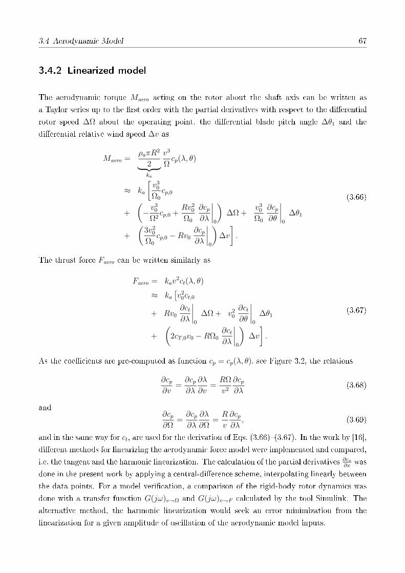
3.4 Aerodynamic Model 67
3.4.2 Linearized model
The aerodynamic torque Maero acting on the rotor about the shaft axis can be written as
a Taylor series up to the rst order with the partial derivatives with respect to the dierential
rotor speed ∆Ω about the operating point, the dierential blade pitch angle ∆θ1 and the
dierential relative wind speed ∆v as
Maero =ρaπR
2
2︸ ︷︷ ︸ka
v3
Ωcp(λ, θ)
≈ ka
[v3
0
Ω0
cp,0
+
(− v
30
Ω2cp,0 +
Rv20
Ω0
∂cp∂λ
∣∣∣∣0
)∆Ω +
v30
Ω0
∂cp∂θ
∣∣∣∣0
∆θ1
+
(3v2
0
Ω0
cp,0 −Rv0∂cp∂λ
∣∣∣∣0
)∆v
].
(3.66)
The thrust force Faero can be written similarly as
Faero = kav2ct(λ, θ)
≈ ka[v2
0ct,0
+ Rv0∂ct∂λ
∣∣∣∣0
∆Ω + v20
∂ct∂θ
∣∣∣∣0
∆θ1
+
(2cT,0v0 −RΩ0
∂ct∂λ
∣∣∣∣0
)∆v
].
(3.67)
As the coecients are pre-computed as function cp = cp(λ, θ), see Figure 3.2, the relations
∂cp∂v
=∂cp∂λ
∂λ
∂v=RΩ
v2
∂cp∂λ
(3.68)
and∂cp∂Ω
=∂cp∂λ
∂λ
∂Ω=R
v
∂cp∂λ
, (3.69)
and in the same way for ct, are used for the derivation of Eqs. (3.66)(3.67). In the work by [16],
dierent methods for linearizing the aerodynamic force model were implemented and compared,
i.e. the tangent and the harmonic linearization. The calculation of the partial derivatives ∂c∗∂x
was
done in the present work by applying a central-dierence scheme, interpolating linearly between
the data points. For a model verication, a comparison of the rigid-body rotor dynamics was
done with a transfer function G(jω)vΩ and G(jω)vF calculated by the tool Simulink. The
alternative method, the harmonic linearization would seek an error minimization from the
linearization for a given amplitude of oscillation of the aerodynamic model inputs.

68 3 Development of a Low-Order Simulation Model
PSfrag replacements
Power coefficient cp [-]Thrust coefficient ct [-]
λ [-]θ [deg]
010
2030
010
2030 0
10
0
10
0
0.2
0.4
0
0.5
1
Figure 3.2: Thrust and power coecients of the DTU 10 MW RWT.
The tangent linearization using a rigid disk for the rotor showed a reasonably good agreement
with the reference code FAST, coupled to Aerodyn v14. The fact that such a simple model
delivers satisfying results for FOWTs is because it is able to represent the dynamics of the RHPZ
through the controller, introduced in Section 2.9, and the low-frequency excitation from the
turbulence. These are the dominant aerodynamic eects for FOWTs, whereas the rotor speed
harmonics are either more damped than for onshore turbines, Figure 2.3, or merely of a lower
order of magnitude than the rst-order wind and wave loads. A comparison of the simple model
compared to two other aerodynamic models can be found in Section 6.4.6.
3.5 Hydrodynamic Model
The common approach for FOWT modeling is a time-domain representation with Cummins'
equation, Eq. (2.19), with additional Morison drag forces to represent the viscous forces ne-
glected by potential ow theory, as introduced in Section 2.5.3.
In order to achieve the goal of computational eciency, a simplication of the convolution
integral of Cummins' equation is necessary, avoiding a time-consuming numerical solution and
to obtain an equivalent LTI model. The next sections will introduce the still-water (radiation)
problem, a conventional and a parametric rst-order wave excitation model, before Morison's
equation and the formulation of slowly-varying drift forces is introduced. Special attention is
paid to the linearization of the Morison drag in Section 3.5.4 because rst, the system damping is
important for a robust controller design of Chapter 5 and second, a good drag parameterization
is necessary for the parametric design studies of Chapter 6.
3.5 Hydrodynamic Model 69
3.5.1 Radiation model
A simplication of the radiation problem in numerical representations has been subject to
research for many years. One example is the approximation of the radiation force dynamics
with a parametric LTI model as described in the introduction, Section 2.5.3. In this case, a
dynamic model is tted to the dynamics from the motion of the oating body to the resulting
forces on the body itself. The model has a number of states depending on the quality of the t
in each DoF of the oating body. As a consequence, the radiation force model adds a signicant
number of states to the FOWT model (usually 36 states for each DoF).
A dynamic state-space radiation model was implemented for this model according to [101].
However, for the results shown in this work it was not applied. Instead, the frequency-
dependency of the added mass A(ω) is neglected in the present nonlinear time-domain model
and a constant frequency is chosen, at which the added mass matrix is interpolated. This
simple and ecient model has shown very promising results, see Section 6.4.6. With this con-
stant matrix approach, reported in [220], reasonable frequencies have to be selected for the
interpolation to obtain the frequency-independent Ac ≡ A(ωc). In this case, the EQM of a
rigid body of Eq. (2.15) is transformed to the time-domain as
(M +A(ωc))ξ(t) +B(ωc)ξ(t) +Cξ(t) = F (1)(t). (3.70)
One approach is to select the constant frequencies of vector ωc according to the respective
eigenfrequencies of the rigid oating body. This approach has the disadvantage that the solution
is in fact only valid for the selected frequency ωc. Section 6.4.6 will show, however, that the
response deviation at other frequencies is limited. In the present implementation, the coupled
entries of A(ω) are interpolated at the eigenfrequency of the motion-DoF (index i) instead
of the force-DoF (index j). Figure 3.3 shows the frequency-dependent added mass with the
interpolated values.
For the radiation damping matrix B(ω), an interpolation is not possible due to the strong
dependence on the frequency. The nonlinear SLOW model does not include any frequency-
dependent parameters and completely neglects radiation damping. The linear frequency-
domain SLOW model includes the frequency-dependent radiation damping and the frequency-
dependent added mass. The linear state-space description, Eq. (3.49) is solved sequentially for
all frequencies. A drawback is here the signicant computational eort, due to the inversion of
the mass matrix. A comparison of the computational speed for the entire model is shown in
Section 3.9.
As discussed in the introduction, the radiation model has two major eects: One is the
(frequency-dependent) damping due to the radiated waves and the other is a frequency-
dependent added mass. The damping eect is often quite small for FOWTs, compared to

70 3 Development of a Low-Order Simulation Model
11
33
frequency [Hz]A
55
[101
0kgm
2]
frequency [Hz]
A51
[108kgm
]
A15
[107kgm
]
Aii
[107kg]
0 0.1 0.2 0.3 0.40 0.1 0.2 0.3 0.4
2.6
2.7
2.8
2.9
−8
−7
−6
−8
−7
−6
2
4
Figure 3.3: Panel code added mass of TripleSpar platform with values interpolated at respectiveeigenfrequencies.
the viscous damping from ow separation, but the magnitude depends nally on the oater
hull shape. The assessment of Section 6.4.6 shows that the radiation damping is small for the
shapes used in this work. It is commonly large at frequencies outside the rigid-body natural
frequencies. Therefore, radiation damping is neglected for most results of this work.
3.5.2 First-order wave force model
The driving force of the right-hand side of Eq. (2.19) in time-domain, the wave excitation
force F (1)(t), is usually obtained through an IDFT of the wave force spectrum. It is, however,
also possible to derive a parametric transfer function from the wave height (which can be
measured by buoys or radars) to the six forces on a oating body, as introduced in Section 2.5.3.
This new approach was investigated as part of this thesis in order to prepare the necessary
models for model-predictive control including a preview of the incoming waves. Both methods
are presented in the following.
Fourier transform-based model
The six rst-order force amplitude spectra F (1) on a oating body for a given sea state can be
obtained in the frequency-domain by multiplying the force coecient X(ω) with the complex
wave amplitude spectrum ζ0(ω)
F (1)(ω) = X(ω)ζ0(ω). (3.71)
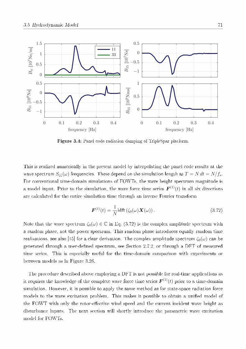
3.5 Hydrodynamic Model 71
11
33
frequency [Hz]B
55
[109Nms]
frequency [Hz]
B51
[108Ns]
B15
[107Ns]
Bii
[107Ns/m
]
0 0.1 0.2 0.3 0.40 0.1 0.2 0.3 0.4
0
0.5
1
−1
−0.5
0
0.5
−1
−0.5
0
0.5
0
0.5
1
1.5
Figure 3.4: Panel code radiation damping of TripleSpar platform.
This is realized numerically in the present model by interpolating the panel code results at the
wave spectrum Sζζ(ω) frequencies. These depend on the simulation length as T = N dt = N/fs.
For conventional time-domain simulations of FOWTs, the wave height spectrum magnitude is
a model input. Prior to the simulation, the wave force time series F (1)(t) in all six directions
are calculated for the entire simulation time through an inverse Fourier transform
F (1)(t) =1
Nidft (ζ0(ω)X(ω)) . (3.72)
Note that the wave spectrum ζ0(ω) ∈ C in Eq. (3.72) is the complex amplitude spectrum with
a random phase, not the power spectrum. This random phase introduces equally random time
realizations, see also [15] for a clear derivation. The complex amplitude spectrum ζ0(ω) can be
generated through a user-dened spectrum, see Section 2.7.2, or through a DFT of measured
time series. This is especially useful for the time-domain comparison with experiments or
between models as in Figure 3.26.
The procedure described above employing a DFT is not possible for real-time applications as
it requires the knowledge of the complete wave force time series F (1)(t) prior to a time-domain
simulation. However, it is possible to apply the same method as for state-space radiation force
models to the wave excitation problem. This makes it possible to obtain a unied model of
the FOWT with only the rotor-eective wind speed and the current incident wave height as
disturbance inputs. The next section will shortly introduce the parametric wave excitation
model for FOWTs.
72 3 Development of a Low-Order Simulation Model
Parametric model
This section deals with the system identication of the frequency-dependent wave excitation
force coecient X(ω) as presented in [103]. It is originally calculated by 2D strip-theory
or 3D panel codes employing linear potential ow theory. The force vector X(ω) contains two
components: The Froude-Krylov force due to the incident wave pressure on the hull and the
force due to diraction of the wave eld. The diculty of tting the wave excitation force to
an LTI model is the fact that the wave height ζ0, used as reference in the panel code for the
calculation of X(ω), is the wave height at the longitudinal position of the FOWT CF. This
results in a non-causal transfer function, which means that the forces might arrive at the
oating body prior to the wave elevation. In this case the disturbance model input ζ0 would
no longer be the cause for the output, the wave excitation force. Potential ow theory shows
that ocean waves are dispersive, i.e. they travel at dierent phase velocities vp depending on
the wavenumber k, see Section 2.5.3. When selecting a wave height sensor position at some
distance from the body against the wave heading direction, the wave excitation force model
can be made causal. Falnes has elaborated this problem comprehensively in [221].
A system identication approach will be followed with an impulse response being subject to
the t of a parametric model. see [222]. The next sections will address the causalization of the
wave excitation force and the model t.
Causalization The wave excitation problem, or the wave excitation transfer function will now
be modied to obtain a causal relationship between the wave height ζ0 and the six forces on the
platform F (1). Figure 3.5 shows the response of the wave excitation force coecient X(ω) to a
wave height impulse at t = 0 s in red. The response has been calculated through an IDFT of the
wave excitation force coecientX(ω). It can be seen that there is a response at negative times,
showing the non-causality as described above. A model t of a non-causal transfer function is
not possible and therefore, as discussed above and in [221], a time delay τc will be introduced
in order to make sure that the transfer function GF,i ≡ GζFi is causal for all directions i.
The time delay τc is the time by which the causalized impulse response is lagged compared
to the original one. This means that the response time of the causalized system is tc = t− τc.Thus, a wave height time series at the position of the platform at time t yields its physically
corresponding wave force response at the time tc. In frequency-domain, the time delay τc is
converted to a frequency-dependent phase lag ϕc(ω) as
ϕc(ω) = ω τc. (3.73)
The time delay τc, selected for the OC3-Hywind spar in Figure 3.5 is τc = 6 s.
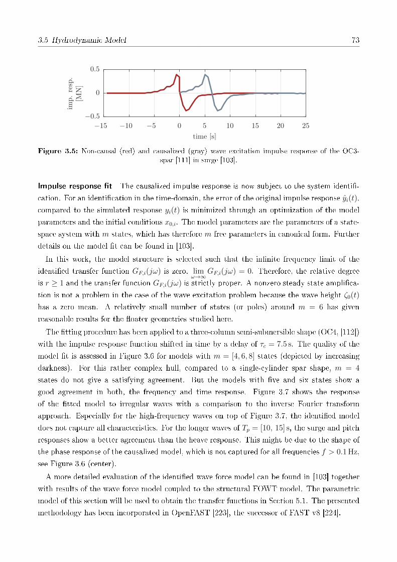
3.5 Hydrodynamic Model 73
time [s]
imp.
resp
.
[MN]
−15 −10 −5 0 5 10 15 20 25
−0.5
0
0.5
Figure 3.5: Non-causal (red) and causalized (gray) wave excitation impulse response of the OC3-spar [111] in surge [103].
Impulse response t The causalized impulse response is now subject to the system identi-
cation. For an identication in the time-domain, the error of the original impulse response yi(t),
compared to the simulated response yi(t) is minimized through an optimization of the model
parameters and the initial conditions x0,i. The model parameters are the parameters of a state-
space system with m states, which has therefore m free parameters in canonical form. Further
details on the model t can be found in [103].
In this work, the model structure is selected such that the innite frequency limit of the
identied transfer function GF,i(jω) is zero, limω→∞
GF,i(jω) = 0. Therefore, the relative degree
is r ≥ 1 and the transfer function GF,i(jω) is strictly proper. A nonzero steady state amplica-
tion is not a problem in the case of the wave excitation problem because the wave height ζ0(t)
has a zero mean. A relatively small number of states (or poles) around m = 6 has given
reasonable results for the oater geometries studied here.
The tting procedure has been applied to a three-column semi-submersible shape (OC4, [112])
with the impulse response function shifted in time by a delay of τc = 7.5 s. The quality of the
model t is assessed in Figure 3.6 for models with m = [4, 6, 8] states (depicted by increasing
darkness). For this rather complex hull, compared to a single-cylinder spar shape, m = 4
states do not give a satisfying agreement. But the models with ve and six states show a
good agreement in both, the frequency and time response. Figure 3.7 shows the response
of the tted model to irregular waves with a comparison to the inverse Fourier transform
approach. Especially for the high-frequency waves on top of Figure 3.7, the identied model
does not capture all characteristics. For the longer waves of Tp = [10, 15] s, the surge and pitch
responses show a better agreement than the heave response. This might be due to the shape of
the phase response of the causalized model, which is not captured for all frequencies f > 0.1 Hz,
see Figure 3.6 (center).
A more detailed evaluation of the identied wave force model can be found in [103] together
with results of the wave force model coupled to the structural FOWT model. The parametric
model of this section will be used to obtain the transfer functions in Section 5.1. The presented
methodology has been incorporated in OpenFAST [223], the successor of FAST v8 [224].

74 3 Development of a Low-Order Simulation Model
pitchheavesurge
time [s]time [s]time [s]
For
ceim
p.
resp
onse
[MN]
frequency [Hz]frequency [Hz]frequency [Hz]
∠Gζ
F
[deg]
|Gζ
F|
[MN]/[M
Nm]
0 10 20 300 10 20 300 10 20 30
0 0.1 0.2 0.30 0.1 0.2 0.30 0.1 0.2 0.3
−10
0
10
−0.2
0
0.2
0.4
−2
−1
0
1
−180
0
180
−180
0
180
−180
0
1800
50
100
0
2
4
0
5
Figure 3.6: Panel code (blue), causalized (red), model t with m = [4, 6, 8] states (gray, increasingdarkness), OC4 semi-submersible [103].
3.5.3 Transformation of hydrodynamic coecients
The panel code calculations are usually done with respect to the oater CF as discussed in
Section 3.2.1 on the formulation of the MBS mass matrices. The convention for the rigid
bodies of the MBS, however, is to dene all properties with respect to their CM. Therefore,
the hydrodynamic coecients A(ω), B(ω) and X(ω) need to be transformed from the CF to
the platform CM. This can be done with the system transformation matrix H(rp) with rp =
[0, 0,−zcm]T , see [225, p. 176]. The matrix reads
H(rp) =
E
3×3 S (rp)T
03×3 E3×3
. (3.74)
The transformation of the added mass matrix follows (for all frequencies) as
Acm = H−T (rp)AcfH−1(rp) (3.75)
and the transformations of B(ω) and X(ω) work equally through a linear transformation.

3.5 Hydrodynamic Model 75
PSfrag replacements
pitchheavesurge
time [s]time [s]time [s]
resp
.Tp=15
s
[MN/M
Nm]
resp
.Tp=10
s
[MN/M
Nm]
resp
.Tp=5s
[MN/M
Nm]
50 100 15050 100 15050 100 150
−200
0
200
−2
0
2
−10
0
10−200
0
200
−5
0
5
−10
0
10−100
0
100
−2
0
2
−10
0
10
Figure 3.7: Wave force response by inverse Fourier transform (black) and 6-state tted model (gray)for Tp = [5, 10, 15] s, OC4 semi-submersible, [103].
3.5.4 Morison's equation
For the modeling of viscous drag forces, Cummins' equation with the linear panel code coe-
cients needs to be augmented with Morison's quadratic drag term. This is the main objective
of this section, although Morison's full equation has been implemented in the model. The
implementation accounts for viscous damping as well as drag-induced excitation forces. A pub-
lication, dedicated to the application of Morison's equation with the linearized SLOW-model
of this work can be found in [226].
The drag coecients CD for cylindrical structures in horizontal cross-ow can be found in the
literature, e.g [227]. They depend usually on the Keulegan-Carpenter KC and the Reynolds
number Re, see Eqs. (2.12) and (2.40) in the introduction. Although Morison's equation (2.21)
provides only horizontal forces, a quadratic drag term can be applied to heave plates in vertical
direction. Chapter 4 on the experiments will deal more in detail with the identication of the
drag coecients of the dierent members of the oater. Exemplary results are shown in this
section for the scaled TripleSpar model of Chapter 4 and the full-scale TripleSpar, introduced
in Section 2.10 and subject of Chapter 6.
The next sections will rst address the nonlinear implementation of Morison's equation and
subsequently the linearization procedure.
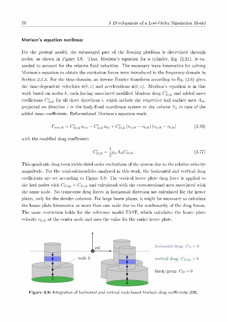
76 3 Development of a Low-Order Simulation Model
Morison's equation nonlinear
For the present model, the submerged part of the oating platform is discretized through
nodes, as shown in Figure 3.8. Thus, Morison's equation for a cylinder, Eq. (2.21), is ex-
tended to account for the relative uid velocities. The necessary wave kinematics for solving
Morison's equation to obtain the excitation forces were introduced in the frequency-domain in
Section 2.5.3. For the time-domain, an inverse Fourier transform according to Eq. (2.6) gives
the time-dependent velocities v(t, z) and accelerations a(t, z). Morison's equation is in this
work based on nodes k, each having associated modied Morison drag C∗D,ik and added mass
coecients C∗A,ik for all three directions i, which include the respective hull surface area Aik,
projected on direction i in the body-xed coordinate system or the volume Ok in case of the
added mass coecients. Reformulated Morison's equation reads
Fmor ,ik = C∗M,ik aw,i − C∗A,ik ab,i + C∗D,ik (vw,ik − vb,ik) |vw,ik − vb,ik| (3.76)
with the modied drag coecients
C∗D,ik =1
2ρwAikCD,ik. (3.77)
This quadratic drag term yields third-order excitations of the system due to the relative velocity
magnitude. For the semi-submersibles analyzed in this work, the horizontal and vertical drag
coecients are set according to Figure 3.8: The vertical heave plate drag force is applied to
the keel nodes with CD,hp = CD,zk and calculated with the cross-sectional area associated with
the same node. No transverse drag forces in horizontal direction are calculated for the heave
plates, only for the slender columns. For large heave plates, it might be necessary to calculate
the heave plate kinematics at more than one node due to the nonlinearity of the drag forces.
The same restriction holds for the reference model FAST, which calculates the heave plate
velocity vb,zk at the center node and uses the value for the entire heave plate.
ref horizontal drag: CD > 0
vertical drag: CD,hp > 0
black/green: CD = 0
node k
Figure 3.8: Integration of horizontal and vertical node-based Morison drag coecients [226].

3.5 Hydrodynamic Model 77
The modied inertia coecients are dened as
C∗M,ik = ρwOk(1 + CA,ik) = C∗A,ik + ρwOk. (3.78)
The modied added mass coecient C∗A,ik, related to the body acceleration, is in the reduced-
order model already included in the structural mass matrix in order to avoid forces dependent
on the generalized accelerations (which are on the left-hand side of the EQM, Eq. (3.16) and
therefore only known for the previous integration step). For heave plates, the modied added
mass coecient is usually referenced with the volume of a half sphere as
C∗A,zk =2
3πr3
i ρwCA,zk. (3.79)
Although the vertical Froude-Krylov forces are not part of Morison's equation, they are also
calculated based on the nodes in Figure 3.8: For every submerged surface having a projected
horizontal component Azk, a node k is dened giving the force Ffk,zk. The dynamic Froude-
Krylov pressure is calculated based on linear wave theory using deep water approximation
as
Ffk,zk(ω) = Azkζ0(ω)e−k(ω)zk . (3.80)
The drag-excitation part poses a challenge for the time-domain model in satisfying the ini-
tial goal of Section 3.1 because no measurable, scalar, time-dependent disturbance can be fed
to the force model of Morison's equation. Instead, an IDFT is necessary, based on a wave
height spectrum. Within this work, simplications have been tested, i.e. assuming the wave
height is a narrow-banded stochastic process such that Eqs. (2.8)(2.10) can be solved for a
constant frequency and a constant wavenumber k = kp = (2π/Tp)2/g, calculated at the peak
spectral period Tp. With this simplication it is possible to calculate the wave kinematics in
vertical and horizontal direction as a function of the incident wave height ζx(t) and its deriva-
tive ζx(t) = dζx/dt at the longitudinal location x (assuming the wave heading direction is x). In
spite of these advantages, the nonlinear dispersion relationship of Eq. (2.4) produces a quadratic
dependency between the wavenumber k and the wave angular frequency ω, yielding large errors
for frequencies outside the selected narrow band of frequencies. Especially in heave-direction,
the Froude-Krylov force transfer function decays quickly with increasing frequencies such that
the simplication yields large errors in the low-frequency regime. As a consequence, the sim-
plication is not employed in the present study but the wave kinematics are calculated a-priori
from an IDFT. The implementation of the Morison model for Linear Model-Predictive Control
(MPC) with a disturbance measurement input for the waves needs further investigation.
For the linearized frequency-domain FOWT model, a linear transfer function will be derived
in the following with a linearizaton of the quadratic Morison drag term.

78 3 Development of a Low-Order Simulation Model
Morison's equation linearized
Morison's equation contains external excitation forces (all summands of Eq. (3.76) which are a
function of the wave kinematics, subscript w) and damping forces (all summands of Eq. (3.76),
which are a function of the body velocity, subscript b). This nonlinear drag term is a challenge
for the linearization. A recent publication by Pegalajar-Jurado [96] presents a method, simpli-
fying the quadratic problem of relative velocities. Although the linearization method selected
in this work is dierent, it also separates the external forcing and the damping terms.
All external forcing terms of Morison's equation (velocity and acceleration-dependent) can be
written as a transfer function within the linearized model. With the water velocity vw(ω, x, z)
and the water acceleration aw(ω, x, z) from Eqs. (2.8)(2.10), the transfer functions from wave
height ζ0 at the initial position to the three translational (superscript t) forces on the CF are
GtFmor(ω) =
∑
k=1
(Cw∗D,ikvw,ik + C∗M,ikaw,ik
) 1
ζ0(ω). (3.81)
The overline denotes the linearized drag coecients to be identied. For the transfer function
in rotational direction (superscript r) from ζ0 to the three moments on the platform about
the CF remains
GrFmor(ω) =
∑
k=1
rik ×GtFmor(ω), (3.82)
the cross product with the position vector rik to each node k. Note that it has shown to
be important to calculate the wave kinematics at the longitudinal positions of the respective
member of node k, see Eq. (2.5). A comparison of the acceleration-dependent parts (Froude-
Krylov forces, last two summands of Eq. (3.81)) using Morison's approach with the potential
ow approach is shown next, before the linearization to obtain the equivalent coecients Cw∗D,ik
is addressed.
Froude-Krylov excitation The transfer functions for the Froude-Krylov (acceleration-
dependent) part are shown in Figure 3.9, without the velocity-dependent part, in order to
compare to the panel code results. Here, the added mass coecients C∗A,ik are chosen such
that the integral added mass from the panel code results equals the added mass from Mori-
son's equation. It can be seen that there is a fairly good agreement for low frequencies. In
the introduction, a limit of ka = 0.5 was given, above which diraction becomes important,
see Figure 2.4. The diraction limit is here 0.997 Hz for ka = 0.5. Beyond this frequency the
agreement is poor, especially in surge-direction. The wiggles result from the dependence of the
kinematics on the longitudinal position and represent the interference of the wave length with
the oater members, Eq. (2.5). The linearization of the (velocity-dependent) drag coecients
for the excitation part is subject of the next section, followed by the drag-induced damping.

3.5 Hydrodynamic Model 79
PSfrag replacements
frequency [Hz]
∠G55
Fmor(ω
)
[deg]
frequency [Hz]
|G55
Fmor(ω
)|[N
m/m
]
∠G33
Fmor(ω
)
[deg]
|G33
Fmor(ω
)|[N
/m]
∠G11
Fmor(ω
)
[deg]
|G11
Fmor(ω
)|[N
/m]
0 1 2 3 40 1 2 3 4
0
500
1000
0
500
10000
1000
2000
0
1000
20000
500
1000
0
2000
4000
Figure 3.9: Morison excitation transfer functions GFmor (ω) for Froude-Krylov component only (blue)compared to panel code transfer functions X(ω) (orange), scaled TripleSpar of Chapter 4.
Drag linearization Various procedures for the linearization of the drag term of Eq. (3.76)
have been proposed, mainly for stationary vertical cylinders. The general challenge of a correct
modeling of the drag forces is the dependence of the quadratic coecients CD on the relative
ow around the body, usually quantied through Re and KC , see Section 2.5.3. The ow
situation, on the other hand, depends on the sea state, the member shape and its motion
response. So does the relative velocity about which the quadratic drag CD is linearized depend
on these parameters. Chapter 4 on the experimental tests will deal more in detail with the
determination of the Morison drag coecients.
For the linearization itself, the method most commonly used in literature, following
Borgman [46], is based on the standard deviation of the relative uid velocity. A discussion on
the method with a comparison to alternatives can be found in [228]. The authors conclude that
Borgman's method underestimates the Morison force for ows around cylindrical structures,
dominated not by inertia but by drag forces. A dierent method, minimizing the residual be-
tween the linear and nonlinear response, was presented by [229] and applied to FOWTs in [16].
In this work, a procedure was developed for the damping part as well as the drag excitation
part of Morison's equation employing Borgman's formula.
The velocity-dependent term of Morison's equation (3.76) includes one part contributing
to the external uid velocity-induced or viscous drag-induced excitation and one part related
to the damping. An ecient method for the linearization of the velocity-dependent part of
Eq. (3.76) is selected: The nonlinear drag coecient CD,ik is split into a wave-velocity and
80 3 Development of a Low-Order Simulation Model
a body-velocity dependent part. The velocity-dependent linearized nodal Morison force FD ,ik
results with the approximation as
FD ,ik = Cw∗D,ikvw,ik − Cb∗
D,ikvb,ik (3.83)
in direction i. The part related to the external drag-excitation is (Cw∗D,ikvw,i), and the damping
part is (−Cb∗D,ikvb,i). While the cross-correlation between uid and body velocity is neglected in
Eq. (3.83), it is respected for the identication of the linearized coecients Cw∗D,ik and C
b∗D,ik.
Following [46], the linearized drag coecients CD,ik for wave and body velocities are based on
the STD σ(vik) of the scalar velocity in direction i of a node k with characteristic cross-sectional
area Aik, normal to direction i, as
C∗D,ik =
√8
πσ(vw,ik − vb,ik)
1
2ρwAi,kCD,ik. (3.84)
In the following both, the part representing an external forcing and subsequently the damping
part of Eq. (3.83) will be addressed. Additionally, a parameterized formulation of the quadratic
drag coecient CD for heave plates is implemented, as a function of the KC -number. This is
possible because the drag forces from ow around the edges is usually not Re-dependent.
Drag excitation For the linearization according to Eq. (3.84), the actual relative uid ve-
locity STD is necessary. However, this is dicult as the body response is not yet known. In
order to avoid an iterative procedure, a rst approach is to consider a stationary body for the
identication of the excitation problem. The drag force transfer function GFmor(ω) for the
velocity-dependent components is shown in Figure 3.10 for surge, heave and pitch. Looking at
the magnitudes it can be seen that for the TripleSpar, the velocity-induced excitation is very
small, approximately 20 times smaller than the Froude-Krylov forcing of Figure 3.9.
Next to the above approach, an improved alternative method for obtaining the relative uid
velocities in Eq. (3.84) was implemented: Here, the cross-spectral density matrix of the gener-
alized velocities S ξ(ω) in the 2D xz-plane with the reference point SWL is used, see Eq. (2.14).
To obtain these, the generalized body velocity response spectrum is calculated with the panel
code RAO. Equation (2.15) is dierentiated to obtain the generalized velocity transfer function
Gζξ(ω) = jωξ(ω)
ζ0(ω)(3.85)
and the cross-spectral density matrix for the generalized platform velocities becomes
S ξξ(ω) = Gζξ(ω)SζζG∗Tζξ
(ω). (3.86)
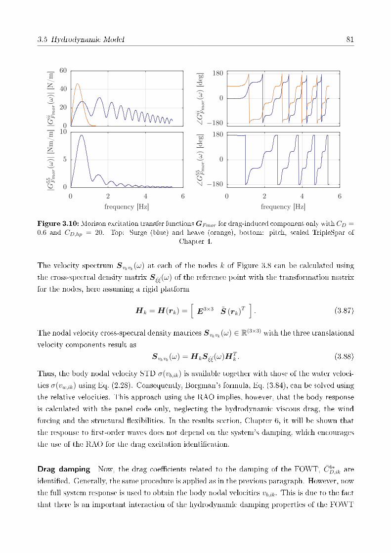
3.5 Hydrodynamic Model 81
PSfrag replacements
frequency [Hz]∠G
55
Fmor(ω
)[d
eg]
frequency [Hz]
|G55
Fmor(ω
)|[N
m/m
]
∠Gii Fmor(ω
)[d
eg]
|Gii Fmor(ω
)|[N
/m]
0 2 4 60 2 4 6
−180
0
180
0
5
10−180
0
180
0
20
40
60
Figure 3.10:Morison excitation transfer functionsGFmor for drag-induced component only with CD =0.6 and CD,hp = 20. Top: Surge (blue) and heave (orange), bottom: pitch, scaled TripleSpar of
Chapter 4.
The velocity spectrum Svkvk (ω) at each of the nodes k of Figure 3.8 can be calculated using
the cross-spectral density matrix S ξξ(ω) of the reference point with the transformation matrix
for the nodes, here assuming a rigid platform
Hk = H(rk) =[E3×3 S (rk)
T]. (3.87)
The nodal velocity cross-spectral density matrices Svkvk (ω) ∈ R(3×3) with the three translational
velocity components result as
Svkvk (ω) = HkS ξξ(ω)HTk . (3.88)
Thus, the body nodal velocity STD σ(vb,ik) is available together with those of the water veloci-
ties σ(vw,ik) using Eq. (2.28). Consequently, Borgman's formula, Eq. (3.84), can be solved using
the relative velocities. This approach using the RAO implies, however, that the body response
is calculated with the panel code only, neglecting the hydrodynamic viscous drag, the wind
forcing and the structural exibilities. In the results section, Chapter 6, it will be shown that
the response to rst-order waves does not depend on the system's damping, which encourages
the use of the RAO for the drag excitation identication.
Drag damping Now, the drag coecients related to the damping of the FOWT, Cb∗D,ik are
identied. Generally, the same procedure is applied as in the previous paragraph. However, now
the full system response is used to obtain the body nodal velocities vb,ik. This is due to the fact
that there is an important interaction of the hydrodynamic damping properties of the FOWT

82 3 Development of a Low-Order Simulation Model
PSfrag replacements
CD [-]σ(vb,x) [m/s]
dep
th[m
]
0.01 0.02 0.03 0.04 0.050 0.02 0.04 0.06 0.08
-1
-0.6
-0.3
SWL
Figure 3.11: Nodal transversal body velocity STD over column length (left) and obtained linearizeddrag coecients CD (right) for two sea states, LCs 7 (blue) and LC 9 (orange) of Chapter 4, [226].
and the rotor dynamics and thus, a coupling with the wind turbine controller. The proposed
procedure uses the previously calculated wave force spectra but now an iteration is necessary:
The hydrodynamic damping is updated as a function of the response, until it converges.
For the identication of the system damping from Morison's equation, only the body veloci-
ties are considered and the uid velocity through the wave kinematics theory, Eqn. (2.8)(2.10),
is set to zero. This simplication allows to separate the above excitation force problem from
the present damping problem (which is important for separating the external force calcula-
tion (pre-processing) from the calculation of the system response). The relative nodal veloc-
ity (vw,ik − vb,ik) is usually dominated by the body velocity at the low-frequency eigenmodes
and by the water velocity at the rst-order wave frequencies. Thus, for the identication of the
damping component (important for the low-frequency resonances, see Chapter 4) the negligence
of the wave kinematics can be considered reasonable.
vb,x1 [m/s]
FD,x1
[N]
−0.1 −0.08 −0.06 −0.04 −0.02 0 0.02 0.04 0.06 0.08 0.1
−0.02
−0.01
0
0.01
0.02
Figure 3.12: Nonlinear (light) and linearized (dark) Morison drag force FD ,x1 for two sea states,LCs 7 (gray) and LC 9 (orange) of Chapter 4 with indication of velocity STD, [226].
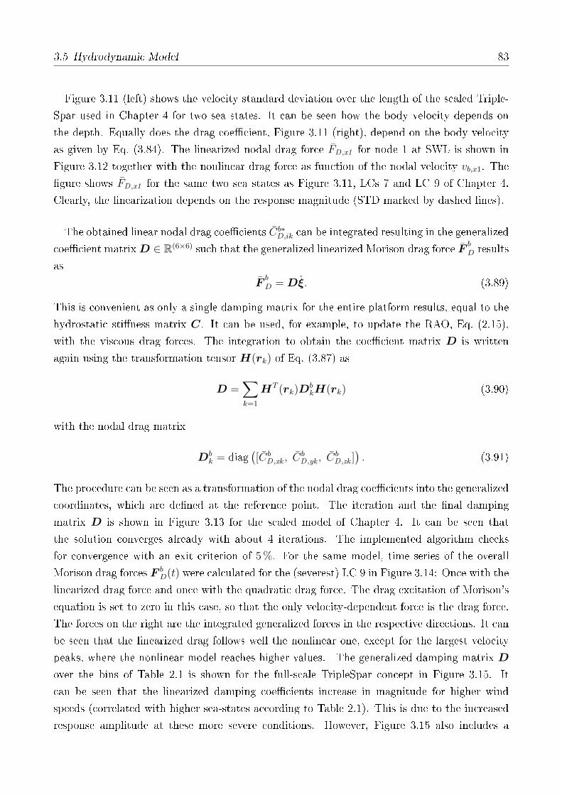
3.5 Hydrodynamic Model 83
Figure 3.11 (left) shows the velocity standard deviation over the length of the scaled Triple-
Spar used in Chapter 4 for two sea states. It can be seen how the body velocity depends on
the depth. Equally does the drag coecient, Figure 3.11 (right), depend on the body velocity
as given by Eq. (3.84). The linearized nodal drag force FD ,x1 for node 1 at SWL is shown in
Figure 3.12 together with the nonlinear drag force as function of the nodal velocity vb,x1. The
gure shows FD ,x1 for the same two sea states as Figure 3.11, LCs 7 and LC 9 of Chapter 4.
Clearly, the linearization depends on the response magnitude (STD marked by dashed lines).
The obtained linear nodal drag coecients Cb∗D,ik can be integrated resulting in the generalized
coecient matrixD ∈ R(6×6) such that the generalized linearized Morison drag force F bD results
as
FbD = Dξ. (3.89)
This is convenient as only a single damping matrix for the entire platform results, equal to the
hydrostatic stiness matrix C. It can be used, for example, to update the RAO, Eq. (2.15),
with the viscous drag forces. The integration to obtain the coecient matrix D is written
again using the transformation tensor H(rk) of Eq. (3.87) as
D =∑
k=1
HT (rk)DbkH(rk) (3.90)
with the nodal drag matrix
Dbk = diag
([Cb
D ,xk , CbD ,yk , C
bD ,zk ]
). (3.91)
The procedure can be seen as a transformation of the nodal drag coecients into the generalized
coordinates, which are dened at the reference point. The iteration and the nal damping
matrix D is shown in Figure 3.13 for the scaled model of Chapter 4. It can be seen that
the solution converges already with about 4 iterations. The implemented algorithm checks
for convergence with an exit criterion of 5 %. For the same model, time series of the overall
Morison drag forces F bD(t) were calculated for the (severest) LC 9 in Figure 3.14: Once with the
linearized drag force and once with the quadratic drag force. The drag excitation of Morison's
equation is set to zero in this case, so that the only velocity-dependent force is the drag force.
The forces on the right are the integrated generalized forces in the respective directions. It can
be seen that the linearized drag follows well the nonlinear one, except for the largest velocity
peaks, where the nonlinear model reaches higher values. The generalized damping matrix D
over the bins of Table 2.1 is shown for the full-scale TripleSpar concept in Figure 3.15. It
can be seen that the linearized damping coecients increase in magnitude for higher wind
speeds (correlated with higher sea-states according to Table 2.1). This is due to the increased
response amplitude at these more severe conditions. However, Figure 3.15 also includes a
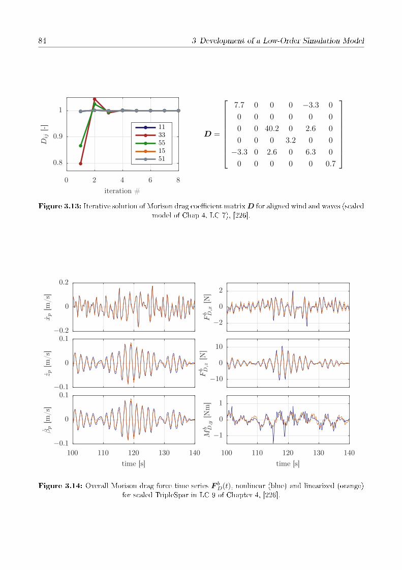
84 3 Development of a Low-Order Simulation Model
11
33
55
15
51
iteration #
Dij
[-]
0 2 4 6 8
0.8
0.9
1
D =
7.7 0 0 0 −3.3 0
0 0 0 0 0 0
0 0 40.2 0 2.6 0
0 0 0 3.2 0 0
−3.3 0 2.6 0 6.3 0
0 0 0 0 0 0.7
Figure 3.13: Iterative solution of Morison drag coecient matrixD for aligned wind and waves (scaledmodel of Chap 4, LC 7), [226].
PSfrag replacements
time [s]
Mb D,y
[Nm
]
time [s]
βp
[m/s
]
Fb D,z
[N]
z p[m
/s]
Fb D,x
[N]
xp
[m/s
]
100 110 120 130 140100 110 120 130 140
−1
0
1
−0.1
0
0.1
−10
0
10
−0.1
0
0.1
−2
0
2
−0.2
0
0.2
Figure 3.14: Overall Morison drag force time series F bD(t), nonlinear (blue) and linearized (orange)
for scaled TripleSpar in LC 9 of Chapter 4, [226].

3.5 Hydrodynamic Model 85
parameterized nonlinear heave plate drag coecient CD,hp, which decreases for larger response
amplitudes. This is the subject of the next paragraph.
Keulegan-Carpenter-dependent drag coecients After the model validation with the ex-
periments, subject of Chapter 4, showed a good agreement with the heave plate drag coecients
from dedicated experiments published in [230], the quadratic drag coecients CD,hp were pa-
rameterized as a function of KC . The drag coecient magnitude as function of KC from
literature data can be seen in Figure 4.12. For heave plates with sharp edges and detached
ow, there is no dependency on Re and the parameterization is more straightforward than for
cylindrical structures with various vortex shedding regimes. The general convergence behavior
shown in Figure 3.13 does not change with the inclusion of the parametric quadratic drag in
the iteration. The resulting heave plate drag coecient can then be used in the same way for
the nonlinear time-domain simulations with the simplied nonlinear model and with FAST.
The iterative frequency-domain solution with KC -dependent heave plate drag is the topic of
the paper [226]. Figure 3.16 shows the KC -dependent resulting quadratic heave plate drag
PSfrag replacements
vhub [m/s]
D55
[GN
ms/
rad]
vhub [m/s]
D51
[MN
s]
D15
[MN
s/ra
d]
D11
[MN
s/m
]
5 10 15 20 255 10 15 20 25
0
0.5
1
−10
−5
0−10
−5
0
0
0.2
0.4
Figure 3.15: Global linearized Morison drag matrix elements for TripleSpar over environmental con-ditions of Table 2.1, [226].
coecients over the operating wind speeds for the full-scale TripleSpar concept. It can be seen
that KC increases for higher wind speeds, which is due to the increasing response amplitude.
As a result, the nonlinear heave plate drag coecient CD,hp decreases for both, the excitation
and the damping problem. The use of a response magnitude-dependent drag coecient is not
common so far but the strong dependency on the LC of Figures 3.15 and 3.16 suggests that
this might be necessary. A summary of the hydrodynamic forcing calculation can be found in
Figure 3.18, including the iterative linearization of the viscous drag forces.
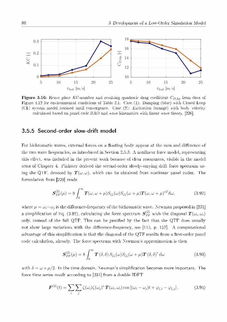
86 3 Development of a Low-Order Simulation Model
PSfrag replacements
vhub [m/s]
CD,hp
[-]
vhub [m/s]
KC
[-]
5 10 15 20 255 10 15 20 25
10
12
14
16
18
0
0.1
0.2
0.3
Figure 3.16: Heave plate KC -number and resulting quadratic drag coecient CD,hp from data ofFigure 4.12 for environmental conditions of Table 2.1. Case (1): Damping (blue) with Closed Loop(CL) system model iterated until convergence. Case (2): Excitation (orange) with body velocity
calculated based on panel code RAO and wave kinematics with linear wave theory, [226].
3.5.5 Second-order slow-drift model
For bichromatic waves, external forces on a oating body appear at the sum and dierence of
the two wave frequencies, as introduced in Section 2.5.3. A nonlinear force model, representing
this eect, was included in the present work because of clear resonances, visible in the model
tests of Chapter 4. Pinkster derived the second-order slowly-varying drift force spectrum us-
ing the QTF, denoted by T (ω, ω), which can be obtained from nonlinear panel codes. The
formulation from [229] reads
S(2)FF (µ) = 8
∫ ∞
0
T (ω, ω + µ)Sζζ(ω)Sζζ(ω + µ)T (ω, ω + µ)∗Tdω, (3.92)
where µ = ωi−ωj is the dierence-frequency of the bichromatic wave. Newman proposed in [231]a simplication of Eq. (3.92), calculating the force spectrum S
(2)FF with the diagonal T (ωi, ωi)
only, instead of the full QTF. This can be justied by the fact that the QTF does usually
not show large variations with the dierence-frequency, see [115, p. 157]. A computational
advantage of this simplication is that the diagonal of the QTF results from a rst-order panel
code calculation, already. The force spectrum with Newman's approximation is then
S(2)FF (µ) = 8
∫ ∞
0
T (δ, δ)Sζζ(ω)Sζζ(ω + µ)T (δ, δ)∗ dω (3.93)
with δ = ω+µ/2. In the time-domain, Newman's simplication becomes more important. The
force time series result according to [231] from a double IDFT
F (2)(t) =∑
i
∑
j
ζ(ωi)ζ(ωj)∗ T (ωi, ωi) cos [(ωi − ωj)t+ ϕζ,i − ϕζ,j] . (3.94)

3.5 Hydrodynamic Model 87
The numerically expensive double summation over ωi and ωj of Eq. (3.94) can be written, as
proposed in [231], as the square of a single sum over suitable frequency ranges. In this case,
the time series result in the formulation of [117] as
F (2)(t) = θ2∣∣T (ωi,ωi)>0
− θ2∣∣T (ωi,ωi)<0
with
θ =∑
i
|ζ(ωi)|√
2|T (ωi, ωi)| cos(ωit+ ϕζ,i),(3.95)
where |ζ(ωi)| is the wave amplitude magnitude at ωi, i.e. from Eq. (2.26), and ϕζ,i is the phase
angle corresponding to the same frequency. In this work, the phase convention is such that ϕ=0
on the positive real axis. The single sum accelerates signicantly the numerical solution. How-
ever, this acceleration comes at the cost of oscillations at high frequencies, appearing in the
force time series. These are not physical and need to be ltered. A further development of
Newman's approximation was proposed by Standing [232] with the product of two sums as
F (2)(t) = Re
([∑
i
|ζ(ωi)| sgn(T (ωi, ωi))√T (ωi, ωi) exp(ωit+ ϕζ,i)
]·
[∑
j
|ζ(ωj)|√T (ωj, ωj) exp(−ωjt+ ϕζ,i)
]). (3.96)
In Figure 3.17, the previously mentioned formulations for the slowly varying drift force of
Eqs. (3.93)(3.96) are compared for a LC of the experiments of Chapter 4 with the 1/60-scaled
TripleSpar of Figure 2.7. The mean drift coecients for the model, calculated with the neareld
solution, are shown in surge-direction in the second plot. The two lower graphs of Figure 3.17
show the force spectra and the corresponding time series. As expected, the drift force spec-
tra S(2)FF ,11 (ω) in surge contain energy outside the frequencies of the wave spectrum Sζζ(ω) (on
top). The direct frequency-domain calculation, Eq. (3.93), predicts the largest response mag-
nitude, especially at low frequencies. The double sum approach of Eq. (3.94) gives slightly
smaller force amplitudes. The above-mentioned unphysical force oscillations can be observed
for Newman's original formulation, Eq. (3.95). They are not present in the improved formula-
tion by Standing, Eq. (3.96). The response magnitude at low frequencies, however, is the same.
The formulation, which is implemented in the model, is the one according to Standing et al.,
Eq. (3.96), the same which is implemented in HydroDyn, see [95] and [117]. For the linearized
frequency-domain model, the spectral densities S(2)FF (ω) are computed through a DFT of the
force time series of Eq. (3.96) in order to ensure equal dierence-frequency excitation for both
models. In conclusion, it is noted that dierences between the various implementations for a
simplied representation of the slowly-varying drift forces exist. A response dierence in the
order of magnitude of Figure 3.17 is also reported in [232, Figure 8]. On the other hand, the dif-
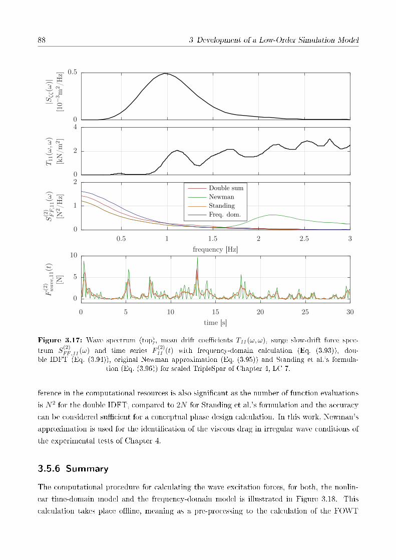
88 3 Development of a Low-Order Simulation Model
Double sum
Newman
Standing
Freq. dom.
time [s]
F(2)
wave,11(t)
[N]
frequency [Hz]
S(2)
FF,11(ω
)
[N2/H
z]
T11(ω
,ω)
[kN
/m2]
|Sζζ(ω
)|[10−
3m
2/H
z]
0 5 10 15 20 25 30
0.5 1 1.5 2 2.5 3
0
5
10
0
1
20
2
40
0.5
Figure 3.17: Wave spectrum (top), mean drift coecients T11 (ω, ω), surge slow-drift force spec-
trum S(2)FF ,11 (ω) and time series F
(2)11 (t) with frequency-domain calculation (Eq. (3.93)), dou-
ble IDFT (Eq. (3.94)), original Newman approximation (Eq. (3.95)) and Standing et al.'s formula-tion (Eq. (3.96)) for scaled TripleSpar of Chapter 4, LC 7.
ference in the computational resources is also signicant as the number of function evaluations
is N2 for the double IDFT, compared to 2N for Standing et al.'s formulation and the accuracy
can be considered sucient for a conceptual phase design calculation. In this work, Newman's
approximation is used for the identication of the viscous drag in irregular wave conditions of
the experimental tests of Chapter 4.
3.5.6 Summary
The computational procedure for calculating the wave excitation forces, for both, the nonlin-
ear time-domain model and the frequency-domain model is illustrated in Figure 3.18. This
calculation takes place oine, meaning as a pre-processing to the calculation of the FOWT

3.5 Hydrodynamic Model 89
response. The forces consist of the rst-order wave force F (1), the slow-drift forces F (2) and
the drag excitation component of Morison's equation Fmor. The nonlinear time-domain model
does not require an oine calculation of the drag excitation from Morison's equation because
it is calculated in each timestep, based on the wave kinematics. In the frequency-domain
model, the Morison excitation forces are included in the pre-processing through the linearized
transfer functions. The linearization is dierent for columns and heave plates because of the op-
tional KC -dependent drag parameterization for the heave plates. The resulting cross-spectral
density matrix of the hydrodynamic excitation forces SFF (ω) can then be used directly to
calculate the response spectra Syy(ω) according to Eq. (2.27). Chapter 4 will deal with the
experimental determination of the Morison drag coecients.
1st order wave force model
• F (1)(t) = idft(X(ω)ζ(ω))
2nd order slow-drift model
• F (2)(t) = idft(idft(ζiζjT (i, i)))
Morison's equation
• wave kinematicsvx(t, z), vz(t, z), ax(t, z), az(t, z)
1st order wave force model
• S(1)FF (ω) = X(ω)Sζζ(ω)X(ω)∗T
2nd order slow-drift model
• S(2)FF (ω) = F (2)(ω)F (2)∗(ω)
Morison's equation
• wave kinematicsvx(ω, z), vz(ω, z), ax(ω, z), az(ω, z)
• body kinematics through RAO(ξζ = X(ω)
−ω2(M+A(ω))+jωB(ω)ξ+C
)
columns
• nodalSTD σ(vi,rel)
• C∗Di =√8πσ(vi,rel)C
∗Di
heave plates (optional)
• nodalSTD σ(vi,rel)
• KCi = f(σi)
• CDi,hp =f(KC), see [230]
• C∗Di =√8πσ(vi,rel)C
∗Di
• GFmor(ω) =∑iHiCD,ie
−kzi
Fζ(t) = F (1)(t) + F (2)(t)
Nonlinear Linear:
SFF (ω) =(GF +GFmor)Sζζ(GF +GFmor)
∗T
Figure 3.18: Overview on calculation scheme for 1st order, 2nd order and Morison (drag componentonly) wave excitation forces as input to nonlinear time-domain model and linear frequency-domain
model. Some formulations are shortened in this overview.
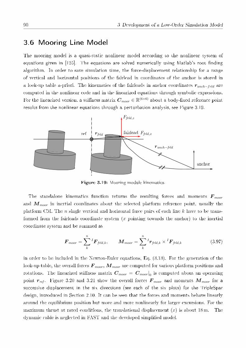
90 3 Development of a Low-Order Simulation Model
3.6 Mooring Line Model
The mooring model is a quasi-static nonlinear model according to the nonlinear system of
equations given in [125]. The equations are solved numerically using Matlab's root nding
algorithm. In order to save simulation time, the force-displacement relationship for a range
of vertical and horizontal positions of the fairlead in coordinates of the anchor is stored in
a look-up table a-priori. The kinematics of the fairleads in anchor coordinates ranch−frld are
computed in the nonlinear code and in the linearized equations through symbolic expressions.
For the linearized version, a stiness matrix Cmoor ∈ R(6×6) about a body-xed reference point
results from the nonlinear equations through a perturbation analysis, see Figure 3.19.
ref rfrld
anchor
fairlead
Ffrld ,z
Ffrld ,x
ranch−frld
Figure 3.19: Mooring module kinematics.
The standalone kinematics function returns the resulting forces and moments Fmoor
and Mmoor in inertial coordinates about the selected platform reference point, usually the
platform CM. The n single vertical and horizontal force pairs of each line k have to be trans-
formed from the fairleads coordinate system (x pointing towards the anchor) to the inertial
coordinate system and be summed as
Fmoor =n∑
k
IF frld ,k , Mmoor =n∑
k
Irfrld ,k × IF frld ,k (3.97)
in order to be included in the Newton-Euler equations, Eq. (3.13). For the generation of the
look-up table, the overall forces Fmoor,Mmoor are computed for various platform positions and
rotations. The linearized stiness matrix Cmoor = Cmoor|0 is computed about an operating
point rref . Figure 3.20 and 3.21 show the overall forces Fmoor and moments Mmoor for a
successive displacement in the six directions (see each of the six plots) for the TripleSpar
design, introduced in Section 2.10. It can be seen that the forces and moments behave linearly
around the equilibrium position but more and more nonlinearly for larger excursions. For the
maximum thrust at rated conditions, the translational displacement (x) is about 18 m. The
dynamic cable is neglected in FAST and the developed simplied model.
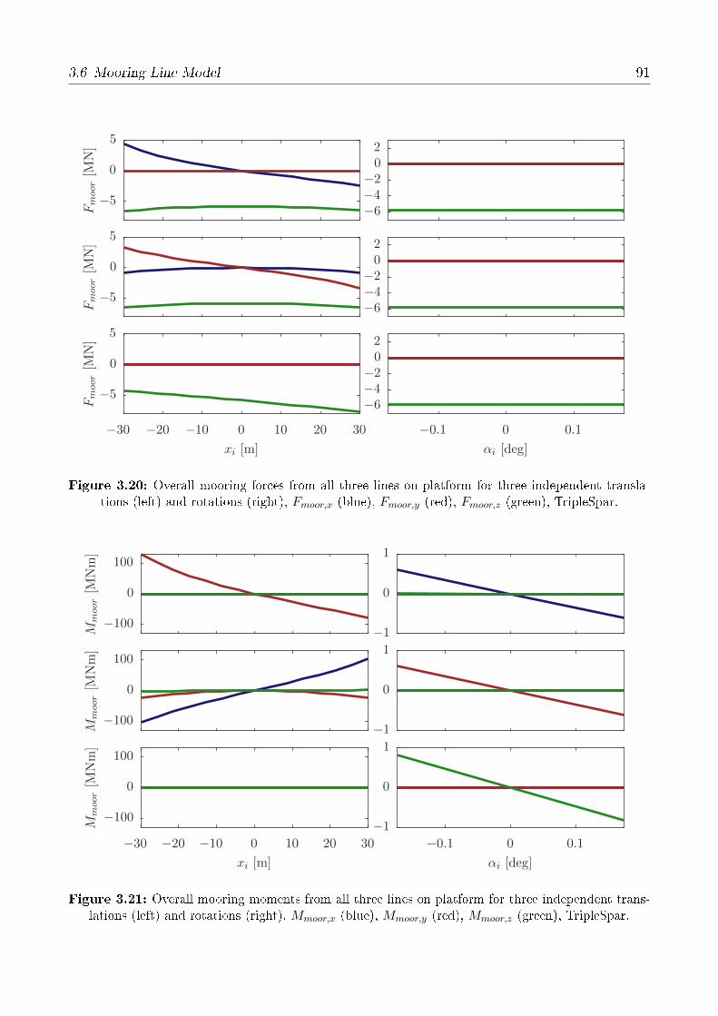
3.6 Mooring Line Model 91
αi [deg]xi [m]
Fmoor[M
N]
Fmoor[M
N]
Fmoor[M
N]
−0.1 0 0.1−30 −20 −10 0 10 20 30
−6−4−202
−6−4−202
−6−4−202
−5
0
5
−5
0
5
−5
0
5
Figure 3.20: Overall mooring forces from all three lines on platform for three independent transla-tions (left) and rotations (right), Fmoor,x (blue), Fmoor,y (red), Fmoor,z (green), TripleSpar.
αi [deg]xi [m]
Mmoor[M
Nm]
Mmoor[M
Nm]
Mmoor[M
Nm]
−0.1 0 0.1−30 −20 −10 0 10 20 30
−1
0
1
−1
0
1
−1
0
1
−100
0
100
−100
0
100
−100
0
100
Figure 3.21: Overall mooring moments from all three lines on platform for three independent trans-lations (left) and rotations (right), Mmoor,x (blue), Mmoor,y (red), Mmoor,z (green), TripleSpar.
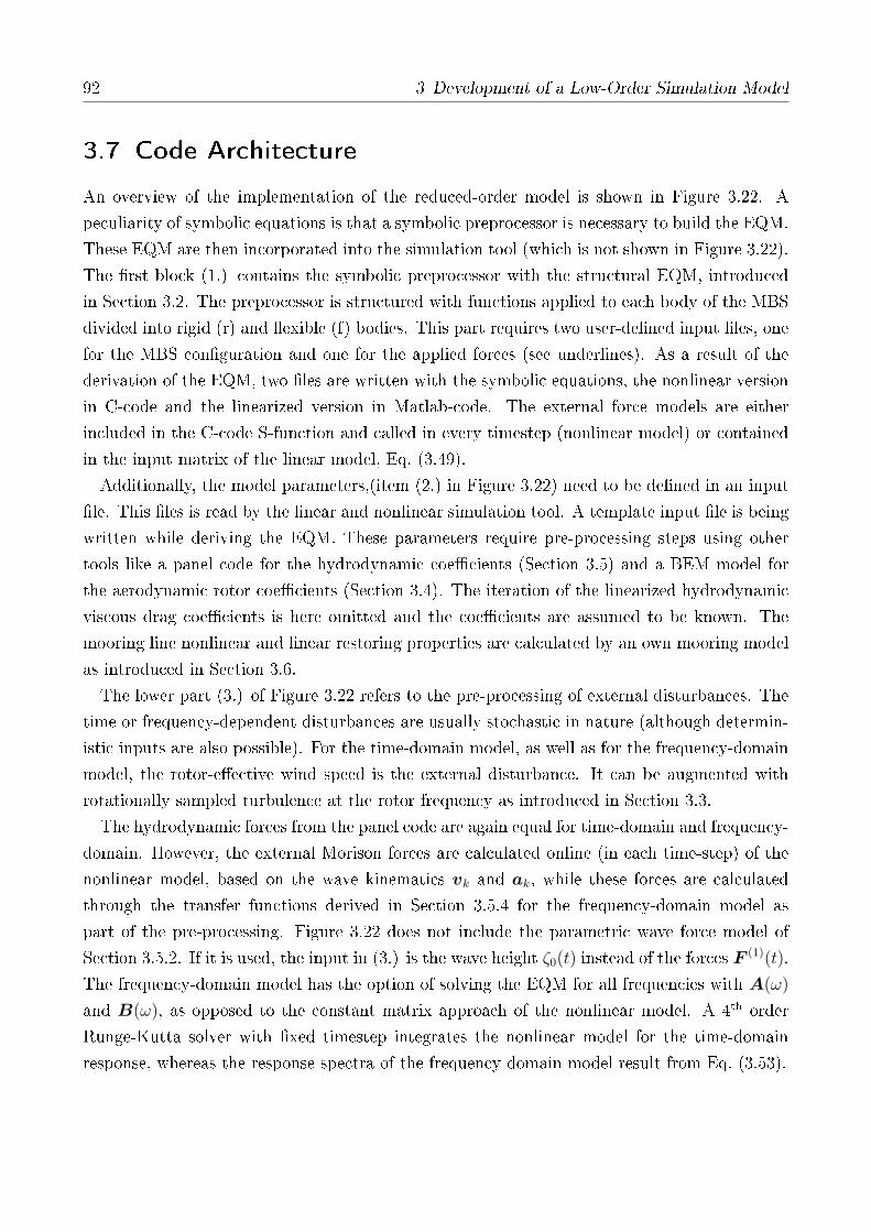
92 3 Development of a Low-Order Simulation Model
3.7 Code Architecture
An overview of the implementation of the reduced-order model is shown in Figure 3.22. A
peculiarity of symbolic equations is that a symbolic preprocessor is necessary to build the EQM.
These EQM are then incorporated into the simulation tool (which is not shown in Figure 3.22).
The rst block (1.) contains the symbolic preprocessor with the structural EQM, introduced
in Section 3.2. The preprocessor is structured with functions applied to each body of the MBS
divided into rigid (r) and exible (f) bodies. This part requires two user-dened input les, one
for the MBS conguration and one for the applied forces (see underlines). As a result of the
derivation of the EQM, two les are written with the symbolic equations, the nonlinear version
in C-code and the linearized version in Matlab-code. The external force models are either
included in the C-code S-function and called in every timestep (nonlinear model) or contained
in the input matrix of the linear model, Eq. (3.49).
Additionally, the model parameters,(item (2.) in Figure 3.22) need to be dened in an input
le. This les is read by the linear and nonlinear simulation tool. A template input le is being
written while deriving the EQM. These parameters require pre-processing steps using other
tools like a panel code for the hydrodynamic coecients (Section 3.5) and a BEM model for
the aerodynamic rotor coecients (Section 3.4). The iteration of the linearized hydrodynamic
viscous drag coecients is here omitted and the coecients are assumed to be known. The
mooring line nonlinear and linear restoring properties are calculated by an own mooring model
as introduced in Section 3.6.
The lower part (3.) of Figure 3.22 refers to the pre-processing of external disturbances. The
time or frequency-dependent disturbances are usually stochastic in nature (although determin-
istic inputs are also possible). For the time-domain model, as well as for the frequency-domain
model, the rotor-eective wind speed is the external disturbance. It can be augmented with
rotationally sampled turbulence at the rotor frequency as introduced in Section 3.3.
The hydrodynamic forces from the panel code are again equal for time-domain and frequency-
domain. However, the external Morison forces are calculated online (in each time-step) of the
nonlinear model, based on the wave kinematics vk and ak, while these forces are calculated
through the transfer functions derived in Section 3.5.4 for the frequency-domain model as
part of the pre-processing. Figure 3.22 does not include the parametric wave force model of
Section 3.5.2. If it is used, the input in (3.) is the wave height ζ0(t) instead of the forces F (1)(t).
The frequency-domain model has the option of solving the EQM for all frequencies with A(ω)
and B(ω), as opposed to the constant matrix approach of the nonlinear model. A 4th order
Runge-Kutta solver with xed timestep integrates the nonlinear model for the time-domain
response, whereas the response spectra of the frequency-domain model result from Eq. (3.53).
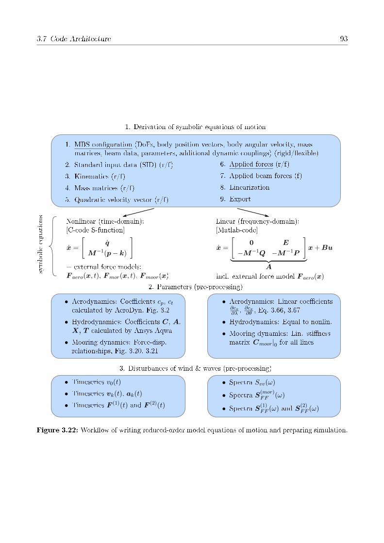
3.7 Code Architecture 93
1. MBS conguration (DoFs, body position vectors, body angular velocity, massmatrices, beam data, parameters, additional dynamic couplings) (rigid/exible)
2. Standard input data (SID) (r/f)
3. Kinematics (r/f)
4. Mass matrices (r/f)
5. Quadratic velocity vector (r/f)
x =
[q
M−1(p− k)
]x =
[0 E
−M−1Q −M−1P
]
︸ ︷︷ ︸A
x+Bu
• Aerodynamics: Coecients cp, ctcalculated by AeroDyn, Fig. 3.2
• Hydrodynamics: Coecients C, A,X, T calculated by Ansys Aqwa
• Mooring dynamics: Force-disp.relationships, Fig. 3.20, 3.21
• Aerodynamics: Linear coecients∂cx∂λ ,
∂cx∂θ , Eq. 3.66, 3.67
• Hydrodynamics: Equal to nonlin.
• Mooring dynamics: Lin. stinessmatrix Cmoor|0 for all lines
• Timeseries v0(t)
• Timeseries vk(t), ak(t)
• Timeseries F (1)(t) and F (2)(t)
• Spectra Svv(ω)
• Spectra S(mor)FF (ω)
• Spectra S(1)FF (ω) and S
(2)FF (ω)
3. Disturbances of wind & waves (pre-processing)
+ external force models:F aero(x, t), Fmor(x, t), Fmoor(x)
Nonlinear (time-domain):[C-code S-function]
Linear (frequency-domain):[Matlab-code]
symbolicequations
1. Derivation of symbolic equations of motion
2. Parameters (pre-processing)
incl. external force model F aero(x)
6. Applied forces (r/f)
7. Applied beam forces (f)
8. Linearization
9. Export
Figure 3.22: Workow of writing reduced-order model equations of motion and preparing simulation.
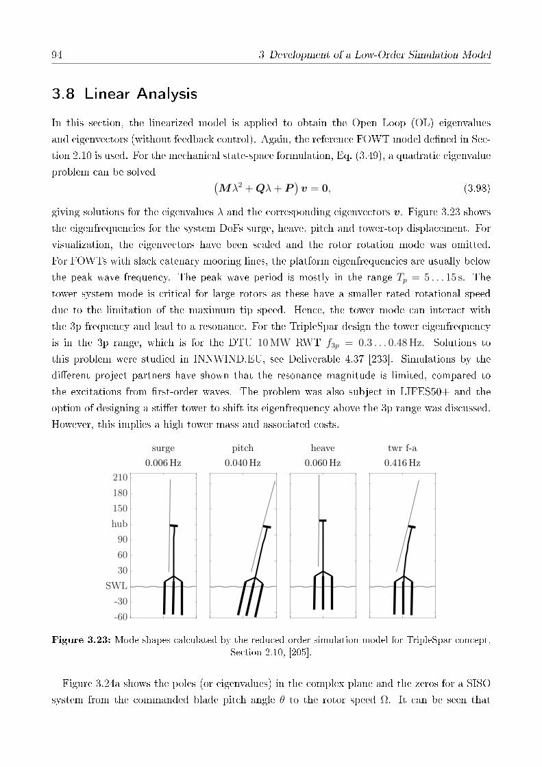
94 3 Development of a Low-Order Simulation Model
3.8 Linear Analysis
In this section, the linearized model is applied to obtain the Open Loop (OL) eigenvalues
and eigenvectors (without feedback control). Again, the reference FOWT model dened in Sec-
tion 2.10 is used. For the mechanical state-space formulation, Eq. (3.49), a quadratic eigenvalue
problem can be solved (Mλ2 +Qλ+ P
)v = 0, (3.98)
giving solutions for the eigenvalues λ and the corresponding eigenvectors v. Figure 3.23 shows
the eigenfrequencies for the system DoFs surge, heave, pitch and tower-top displacement. For
visualization, the eigenvectors have been scaled and the rotor rotation mode was omitted.
For FOWTs with slack catenary mooring lines, the platform eigenfrequencies are usually below
the peak wave frequency. The peak wave period is mostly in the range Tp = 5 . . . 15 s. The
tower system mode is critical for large rotors as these have a smaller rated rotational speed
due to the limitation of the maximum tip speed. Hence, the tower mode can interact with
the 3p frequency and lead to a resonance. For the TripleSpar design the tower eigenfrequency
is in the 3p range, which is for the DTU 10 MW RWT f3p = 0.3 . . . 0.48 Hz. Solutions to
this problem were studied in INNWIND.EU, see Deliverable 4.37 [233]. Simulations by the
dierent project partners have shown that the resonance magnitude is limited, compared to
the excitations from rst-order waves. The problem was also subject in LIFES50+ and the
option of designing a stier tower to shift its eigenfrequency above the 3p range was discussed.
However, this implies a high tower mass and associated costs.
PSfrag replacements
twr f-a
0.416Hz
heave
0.060Hz
pitch
0.040Hz
surge
0.006Hz
-60
-30
SWL
30
60
90
hub
150
180
210
Figure 3.23: Mode shapes calculated by the reduced-order simulation model for TripleSpar concept,Section 2.10, [205].
Figure 3.24a shows the poles (or eigenvalues) in the complex plane and the zeros for a SISO
system from the commanded blade pitch angle θ to the rotor speed Ω. It can be seen that
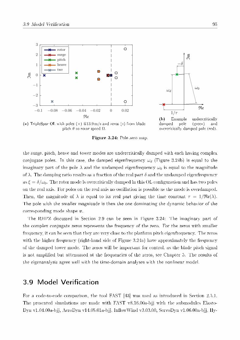
3.9 Model Verication 95
rotor
surge
pitch
heave
twr
Re
Im
−0.1 −0.08 −0.06 −0.04 −0.02 0 0.02
−3
−2
−1
0
1
2
3
(a) TripleSpar OL with poles (×) @13.9 m/s and zeros () from bladepitch θ to rotor speed Ω.
Re
Im
−δ
ωd
1/τ
ω0
(b) Example undercriticallydamped pole (green) andovercritically damped pole (red).
Figure 3.24: Pole-zero map.
the surge, pitch, heave and tower modes are undercritically damped with each having complex
conjugate poles. In this case, the damped eigenfrequency ωd (Figure 3.24b) is equal to the
imaginary part of the pole λ and the undamped eigenfrequency ω0 is equal to the magnitude
of λ. The damping ratio results as a fraction of the real part δ and the undamped eigenfrequency
as ξ = δ/ω0. The rotor mode is overcritically damped in this OL conguration and has two poles
on the real axis. For poles on the real axis no oscillation is possible as the mode is overdamped.
Then, the magnitude of λ is equal to its real part giving the time constant τ = 1/Re(λ).
The pole with the smaller magnitude is then the one dominating the dynamic behavior of the
corresponding mode shape v.
The RHPZ discussed in Section 2.9 can be seen in Figure 3.24: The imaginary part of
the complex conjugate zeros represents the frequency of the zero. For the zeros with smaller
frequency, it can be seen that they are very close to the platform pitch eigenfrequency. The zeros
with the higher frequency (right-hand side of Figure 3.24a) have approximately the frequency
of the damped tower mode. The zeros will be important for control, as the blade pitch signal
is not amplied but attenuated at the frequencies of the zeros, see Chapter 5. The results of
the eigenanalysis agree well with the time-domain analyses with the nonlinear model.
3.9 Model Verication
For a code-to-code comparison, the tool FAST [43] was used as introduced in Section 2.5.1.
The presented simulations are made with FAST v8.16.00a-bjj with the submodules Elasto-
Dyn v1.04.00a-bjj, AeroDyn v14.05.01a-bjj, InowWind v3.03.00, ServoDyn v1.06.00a-bjj, Hy-

96 3 Development of a Low-Order Simulation Model
droDyn v2.05.01 and MAP++ v1.20.10. The enabled features, compared to the nonlinear and
the linearized SLOW model are summarized in Table 3.1.
Table 3.1: Comparison of modeling approaches between FAST, SLOW nonlinear and SLOW linear.
FAST SLOW (nonlinear) SLOW (linear)
Structural
dynamics
nonlin. ex. MBS nonlin. ex. MBS linearized ex. MBS
6 platform DoFs surge, heave, pitch-DoFs surge, heave, pitch-DoFs
4 tower DoFs 1 fore-aft DoF 1 fore-aft DoF
3 · 3 blade DoFs rigid rigid
drivetrain torsional DoF rigid shaft rigid shaft
2nd order blade pitch actuator
Aero-
dynamics
BEM with corrections cp, ct-model (nonlin.) cp, ct-model (lin.)
distrib. forces along blade lumped rotor forces lumped rotor forces
full 3D turb. wind eldblade-averaged wind eld with
rotationally sampled turbulence
quasi-static, no dynamic inow
no tower shadow
Hydro-
dynamics
convolution integral constant matrix frequency-domain
radiation damping radiation damping
relative form of Morison's equation cross-corr. approximated
quadr. Morison drag quadr. Morison drag linearized Morison drag
2nd order slow-drift with Newman's approximation
no wave stretching
Mooring-
dynamics quasi-static model quasi-static model quasi-static model
nonlin. force-disp. nonlin. force-disp. linearized stiness
eq. solved online eq. solved a-priori eq. solved a-priori
The most signicant dierence between the tools is the aerodynamic model and the reduced
number of structural DoFs (2D motion, only). For an improved computational eciency, most
of the results in this work of the linearized model are made without the frequency-dependent hy-
drodynamic coecients but with a constant added mass and neglecting the radiation damping,
see Section 3.5.1.
3.9.1 Stochastic operational condition
Figure 3.25 shows the PSD to stochastic wind and wave loads for a load case
with vhub = 17.9 m/s as described in Section 2.7.3 for the linearized model, the nonlinear model

3.9 Model Verication 97
and FAST. The model includes a SISO PI-controller as described in Chapter 5. All model
parameters can be found in Table A.1. It can be seen that the frequencies of the platform
resonances in surge xp, heave zp and pitch βp are well captured in frequency and magnitude.
The response to the wave loads at fwave = 0.1 Hz can be clearly seen in the xp and xt sig-
nals. The tower-top displacement xt also shows a second peak above the wave frequency,
below its coupled eigenfrequency of 0.42 Hz at about 0.18 Hz. This is due to the wave force
transfer function X(ω), which shows two peaks, divided by an attenuation range, see wave
cancellation eect for semi-submersibles. This can be also seen in Figure 3.6 and is a topic
of Chapter 6. The slow drift force model of Section 2.5.3 results in large amplitudes at the
resonance frequencies of surge xp and pitch βp, also reected in the tower bending xt. Without
this dierence-frequency excitation, the response to the turbulence would be visibly smaller.
The Morison drag coecient for the heave plates CD,hp is obtained according to Section 3.5,
Figure 3.16 with the linear model and its value is used for both nonlinear models.
The rotor speed Ω responds to the βp-motion, which is related to the discussed RHPZ,
Section 2.5. It will be a further topic in the remainder of this work. Since the torque is
constant above rated (vrated = 11.4 m/s), the rotor speed Ω is proportional to the electrical
power P . The tower eigenfrequency is mainly excited by the 3p excitations on the rotor from
the vertical wind shear. It is well captured by the reduced-order model with the rotational
sampling method of Section 3.3. The tower-base bending moment Myt follows generally the
tower-top displacement xt, except for the structural damping force, as discussed in Section 3.2.6.
For a time-domain comparison of the same load case as Figure 3.25, the same turbulent wind
eld was input to SLOW and FAST and the wave height time series ζ0 of FAST were input
to SLOW using Section 3.5.2. The results of Figure 3.26 show in this time-domain comparison
that also the transients and steady states (means) compare well between SLOW and FAST.
The wind speed signal on top shows more high-frequency oscillations for SLOW because of the
rotational sampling, as opposed to the rotor-eective wind speed, shown for FAST. The steady
state deviation of surge (xp) and the blade pitch angle θ is due to the tilted rotor: It has a
nonzero angle about y, through the shaft tilt of 5 deg and through the platform pitching βp. This
misalignment results in nonzero force and moment-components in the directions perpendicular
to the shaft, see Glauert's yaw model in [44, Chapter 3].
3.9.2 Deterministic operational condition
The response of the nonlinear SLOW model and the FAST model to an Extreme Operating
Gust (EOG) at still water can be seen in Figure 3.27. This load case results in large transient
rotor loads and an impulse response-like behavior (the duration of the gust is rather short in the
time-scales of the FOWT). Nonetheless, the nonlinear SLOW model reproduces well the FAST
results. The only visible dierence is the steady state in surge (xp). This is, again, due to the
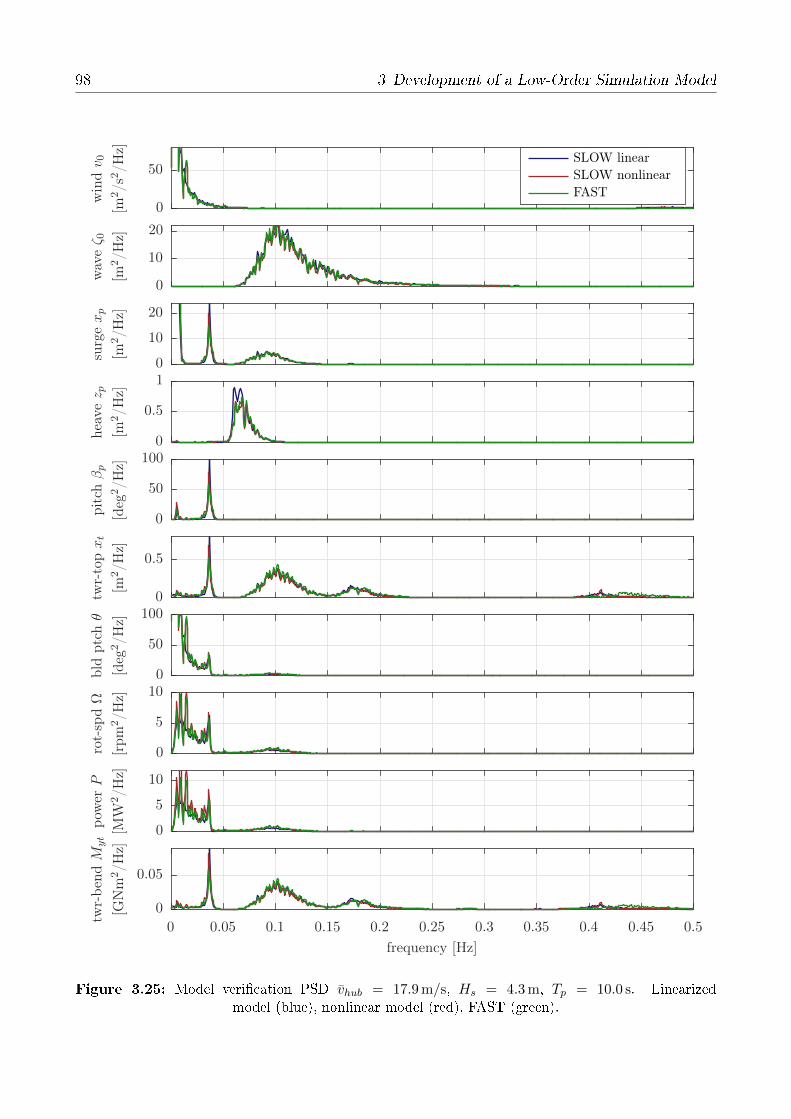
98 3 Development of a Low-Order Simulation Model
PSfrag replacements
SLOW linear
SLOW nonlinear
FAST
frequency [Hz]
twr-
ben
dM
yt
[GN
m2/H
z]
pow
erP
[MW
2/H
z]
rot-
spdΩ
[rpm
2/H
z]
bld
ptc
hθ
[deg
2/H
z]
twr-
topxt
[m2/H
z]
pit
chβp
[deg
2/H
z]
hea
vez p
[m2/H
z]
surg
exp
[m2/H
z]
wav
eζ 0
[m2/H
z]
win
dv 0
[m2/s
2/H
z]
0 0.05 0.1 0.15 0.2 0.25 0.3 0.35 0.4 0.45 0.5
0
0.05
0
5
10
0
5
100
50
1000
0.5
0
50
1000
0.5
10
10
20
0
10
20
0
50
Figure 3.25: Model verication PSD vhub = 17.9 m/s, Hs = 4.3 m, Tp = 10.0 s. Linearizedmodel (blue), nonlinear model (red), FAST (green).
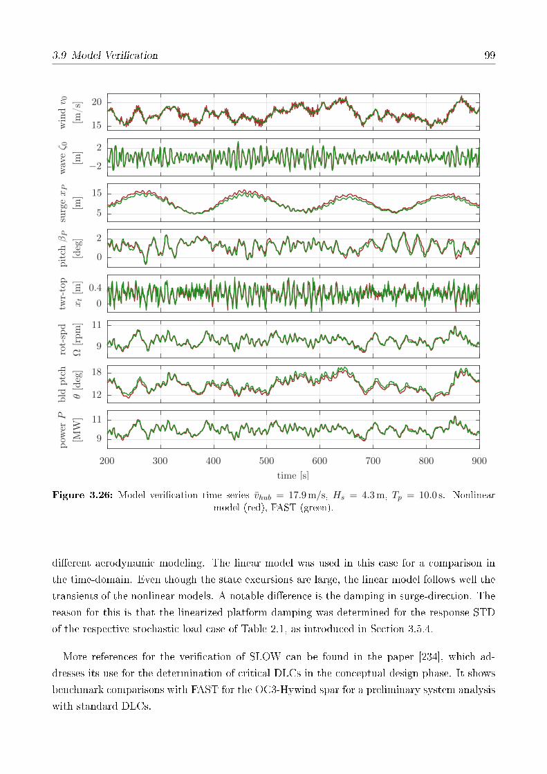
3.9 Model Verication 99
PSfrag replacements
time [s]
pow
erP
[MW
]
bld
ptc
h
θ[d
eg]
rot-
spd
Ω[r
pm]
twr-
top
xt[m
]
pit
chβP
[deg]
surg
exP
[m]
wav
eζ 0
[m]
win
dv 0
[m/s]
200 300 400 500 600 700 800 900
9
11
12
18
9
11
0
0.4
0
2
5
15
−2
2
15
20
Figure 3.26: Model verication time series vhub = 17.9 m/s, Hs = 4.3 m, Tp = 10.0 s. Nonlinearmodel (red), FAST (green).
dierent aerodynamic modeling. The linear model was used in this case for a comparison in
the time-domain. Even though the state excursions are large, the linear model follows well the
transients of the nonlinear models. A notable dierence is the damping in surge-direction. The
reason for this is that the linearized platform damping was determined for the response STD
of the respective stochastic load case of Table 2.1, as introduced in Section 3.5.4.
More references for the verication of SLOW can be found in the paper [234], which ad-
dresses its use for the determination of critical DLCs in the conceptual design phase. It shows
benchmark comparisons with FAST for the OC3-Hywind spar for a preliminary system analysis
with standard DLCs.
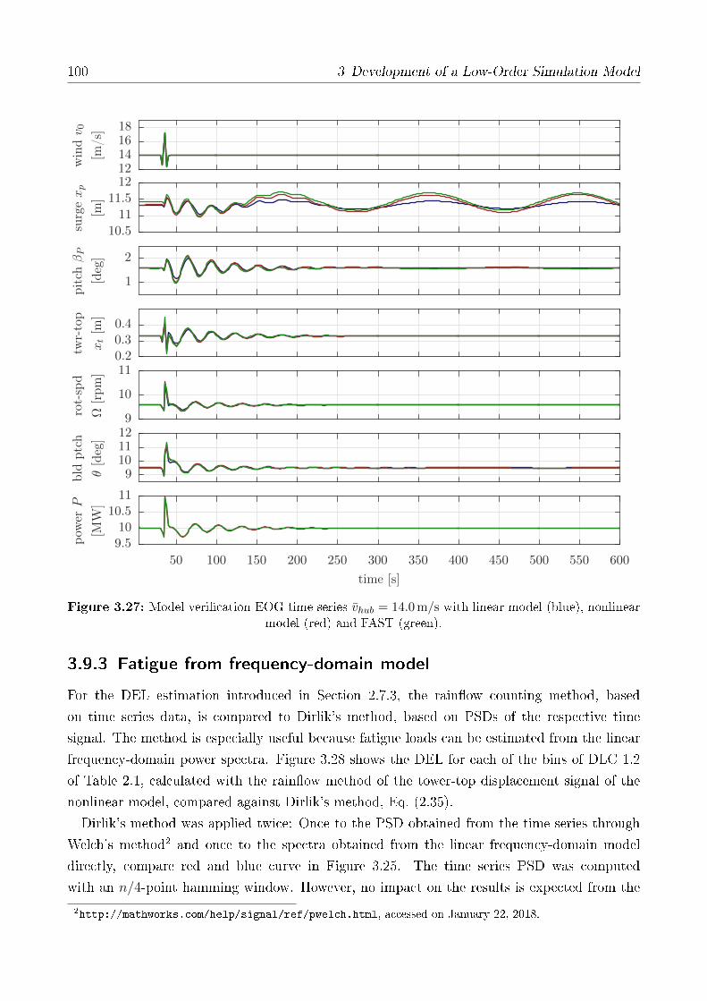
100 3 Development of a Low-Order Simulation Model
PSfrag replacements
time [s]
pow
erP
[MW
]
bld
ptc
h
θ[d
eg]
rot-
spd
Ω[r
pm]
twr-
top
xt[m
]
pit
chβP
[deg]
surg
exp
[m]
win
dv 0
[m/s]
50 100 150 200 250 300 350 400 450 500 550 600
9.510
10.511
91011129
10
110.20.30.4
1
2
10.5
11
11.5
1212141618
Figure 3.27: Model verication EOG time series vhub = 14.0 m/s with linear model (blue), nonlinearmodel (red) and FAST (green).
3.9.3 Fatigue from frequency-domain model
For the DEL estimation introduced in Section 2.7.3, the rainow counting method, based
on time series data, is compared to Dirlik's method, based on PSDs of the respective time
signal. The method is especially useful because fatigue loads can be estimated from the linear
frequency-domain power spectra. Figure 3.28 shows the DEL for each of the bins of DLC 1.2
of Table 2.1, calculated with the rainow method of the tower-top displacement signal of the
nonlinear model, compared against Dirlik's method, Eq. (2.35).
Dirlik's method was applied twice: Once to the PSD obtained from the time series through
Welch's method2 and once to the spectra obtained from the linear frequency-domain model
directly, compare red and blue curve in Figure 3.25. The time series PSD was computed
with an n/4-point hamming window. However, no impact on the results is expected from the
2http://mathworks.com/help/signal/ref/pwelch.html, accessed on January 22, 2018.

3.9 Model Verication 101
windowing due to the large amount of hamming points. The DEL values are calculated for
each bin independently and not weighted but extrapolated for a lifetime of 20 years.
It can be seen that the match is very good with a maximum deviation of only 0.4 % for
the time series data. This conrms Dirlik's method for the nature of the tower-top signal
in the given load conditions. As for the linearization methodology, it does not imply larger
discrepancies than Dirlik's method itself.
Rainflow counting from timeseries
Dirlik from timeseries-PSD
Dirlik from freq.dom.-PSD
v [m/s]
DE
L(x
t)[-]
5.0 7.1 10.3 13.9 17.9 22.1 25.0
0
0.5
1
1.5
2
2.5
Figure 3.28: DEL for tower-top displacement xt for operational DLCs of Table 2.1. Calculated with(1) rainow counting, (2) Dirlik's method with spectra obtained from time series data of (1) and
(3) Dirlik's method with spectra obtained from linearized frequency-domain model.
3.9.4 Short-term extremes from frequency-domain model
It is especially important for controller design to obtain the maximum amplitudes of certain
signals from a 10 min or a 60 min-responses as a performance indicator. In order to be able to
extract these short-term extremes from the linear frequency-domain model, a Rayleigh distri-
bution of the peaks is assumed in order to obtain the expected maximum amplitudes for a given
duration, as introduced in Section 2.7.3. Figure 3.29 shows a comparison, as in Figure 3.28, of
the maximum amplitude (mean of maxima of three 20 min-segments) of the tower-top displace-
ment xt from a time-domain simulation, through the Rayleigh distribution using the PSD of the
time series and through the linear frequency-domain model. It can be seen that the estimation
from the spectrum underestimates the maximum around rated winds, which is likely because
in these cases the signal is not normally distributed. In the other cases the method seems to
give plausible results for the tower bending.

102 3 Development of a Low-Order Simulation Model
MAX from timeseries
MAX from timeseries-PSD
MAX from freq.dom.-PSD
v [m/s]
MA
X(x
t)[-]
5.0 7.1 10.3 13.9 17.9 22.1 25.0
0
0.2
0.4
0.6
0.8
1
Figure 3.29: Short-term extremes for tower-top displacement xt for operational DLCs of Table 2.1.Calculated from (1) time series directly, (2) from PSD of time series and (3) from linear frequency-
domain model response spectrum using Eq. (2.36).
3.10 Computational Eciency
A computational speed assessment is shown in Table 3.2. The simulation times are given for
a standard PC with a 2.5 GHz processor for one hour simulations and n = 500 frequencies for
the linear frequency-domain computations. The pre-processing of wind and waves is necessary
for each load case due to the environmental conditions, cf. Table 2.1. For the SLOW model,
the wave-preprocessing includes the rst-order wave force time series and spectra, the Morison
external drag force spectra and the dierence-frequency spectra and time series using Newman's
approximation, see Section 3.5. The pre-processing of the aerodynamics relates to the BEM-
calculations to determine the look-up tables for cp and ct, Section 3.4. This is only required
once for every new wind turbine rotor. The same holds for the mooring dynamics: The force-
displacement relationships have to be re-calculated only if a new mooring system is employed.
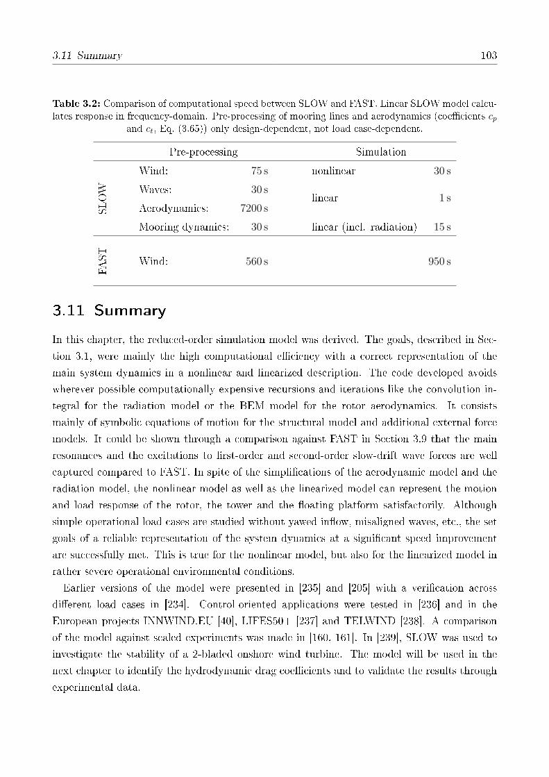
3.11 Summary 103
Table 3.2: Comparison of computational speed between SLOW and FAST. Linear SLOWmodel calcu-lates response in frequency-domain. Pre-processing of mooring lines and aerodynamics (coecients cp
and ct, Eq. (3.65)) only design-dependent, not load case-dependent.
Pre-processing Simulation
SLOW
Wind: 75 s nonlinear 30 s
Waves: 30 slinear 1 s
Aerodynamics: 7200 s
Mooring dynamics: 30 s linear (incl. radiation) 15 s
FAST Wind: 560 s 950 s
3.11 Summary
In this chapter, the reduced-order simulation model was derived. The goals, described in Sec-
tion 3.1, were mainly the high computational eciency with a correct representation of the
main system dynamics in a nonlinear and linearized description. The code developed avoids
wherever possible computationally expensive recursions and iterations like the convolution in-
tegral for the radiation model or the BEM model for the rotor aerodynamics. It consists
mainly of symbolic equations of motion for the structural model and additional external force
models. It could be shown through a comparison against FAST in Section 3.9 that the main
resonances and the excitations to rst-order and second-order slow-drift wave forces are well
captured compared to FAST. In spite of the simplications of the aerodynamic model and the
radiation model, the nonlinear model as well as the linearized model can represent the motion
and load response of the rotor, the tower and the oating platform satisfactorily. Although
simple operational load cases are studied without yawed inow, misaligned waves, etc., the set
goals of a reliable representation of the system dynamics at a signicant speed improvement
are successfully met. This is true for the nonlinear model, but also for the linearized model in
rather severe operational environmental conditions.
Earlier versions of the model were presented in [235] and [205] with a verication across
dierent load cases in [234]. Control-oriented applications were tested in [236] and in the
European projects INNWIND.EU [40], LIFES50+ [237] and TELWIND [238]. A comparison
of the model against scaled experiments was made in [160, 161]. In [239], SLOW was used to
investigate the stability of a 2-bladed onshore wind turbine. The model will be used in the
next chapter to identify the hydrodynamic drag coecients and to validate the results through
experimental data.

4 Experiments
Two test campaigns were performed in the course of this thesis project. One in France in
2014 and one in Denmark in 2016. This chapter describes the latter, performed at the Danish
Hydraulic Institute (DHI) within a joint project by SWE, DTU and CENER in 2016. The
TripleSpar concept introduced in Section 2.10 was built at SWE in a scale of 1/60 and assembled
with a turbine model of the DTU 10 MW RWT, built at DTU, see Figure 4.1. The scaling
laws applied follow Froude-scaling as introduced in Section 2.8. The test campaign had the
primary goal of testing active blade pitch control in a model test and the results were published
in [160], [161] and [240]. Additionally, three thesis projects were conducted on the tests. The one
at SWE by Wei Yu [241] deals with the simulation model setup, the parameter identication,
controller development and implementation. Another one conducted at DTU focused on the
wind generator and the rotor design, see [242] and a Bachelor thesis on the electromechanical
hardware is not published. Prior to this test, most experimental tests of FOWTs did not include
a blade pitch controller. This means that the rotor speed was maintained by a servo motor,
which actuates the torque. However, the gains of this servo controller were usually not tuned to
match the full-scale controller as implemented on standard wind turbines and the blade-pitch
controller was not represented in the tests. As the aerodynamic scaling is challenging, due to
the Reynolds number mismatch the rotor was redesigned for low Re-numbers by DTU in order
to match mainly the Froude-scaled thrust and rotor speed. Recently, a number of researchers
has taken the step to include the control system in scaled model tests after a rst attempt
had been made for the Hywind concept, see [197]. The negative damping problem was studied
in [243]. Later, tests at Marine Research Institute Netherlands (MARIN) with dierent PI-
controllers were presented in [244], assessing the controller inuence on the response. Another
test in the same basin was presented in [245]. At Osaka Prefecture University, Japan, an H∞controller was experimentally studied, see [246].
The objective of this chapter is to validate the previously described hydrodynamic model
and to calibrate the Morison drag coecients. At the same time, comparisons between the
simulation model of Chapter 3 and experimental data with active blade pitch controller will
be shown to validate the full FOWT model. The ndings of this chapter will be used in the
parametric design studies of Chapter 6.

106 4 Experiments
Figure 4.1: TripleSpar test campaign at DHI 2016: Joint project by SWE, DTU and CENER,photograph by Henrik Bredmose, DTU, [240].
Table 4.1: LCs dened for irregular wave tests [160].
Model scale Prototype scaleLC Hs [m] Tp [s] vhub [m/s] Hs [m] Tp [s] vhub [m/s]
1. . . 6, 8, 10 not used, see [241]7 0.091 1.08 1.89 5.46 8.37 14.649 0.159 1.43 1.89 9.54 11.1 14.64
4.1 Model Parameters and Load Cases
The simulation model used for the following analyses is the one described in Chapter 3 with the 5
DoFs platform surge xp, platform heave zp, platform pitch βp, tower fore-aft displacement xt and
rotor speed Ω. The tower is modeled through a linear spring through the rigid MBS approach
of Section 3.2.1. The model parameters used in [161] were not changed, except that the added
mass was calculated with Ansys Aqwa and used in the simulations without further tuning. An
additional linear stiness in x-direction of 8 N/m was introduced to represent the power and
signal cables of the servo motor and blade pitch actuators, which can be seen in Figure 4.1.
This is about one third of the horizontal restoring stiness of the mooring lines in the initial
position. In pitch-direction an additional stiness of −25 Nm/rad was necessary to match the
natural period from the measurements, equal to about 5 % of the hydrostatic restoring in pitch.

4.1 Model Parameters and Load Cases 107
blade pitch θ [deg]
pro
p.
gain
kp
[rad
/rad
/s]
v0 [m/s]
bla
de
pit
chθ
[deg
]
0 2 4 6 8 100 1 2 3
0.1
0.15
0.2
0
5
10
15
20
Figure 4.2: Steady state blade pitch angles θ over wind speeds v0 (left) and proportional gains kpover steady state blade pitch angles (right) associated with time constant Ti = 2.9 s for the 1/60
TripleSpar, [240].
The static vertical force and the vertical stiness of the power cables on the system is neglected.
The model parameters can be found in the Appendix A.2.
The properties of the dierent components of the FOWT system were veried and identied
with dierent methods: For the rotor, a BEM model was set up in the Master thesis [241] with
the polars calculated by DTU and the torque and thrust for dierent TSR were compared to
the measurements as shown in [161]. The tower structural properties were determined for a
xed conguration used in a previous test by DTU, see [247]. For the present work, an impulse
response of the tower-top with the tower mounted on the oating platform was measured. It
resulted in a slightly higher stiness than the one assumed in [161]. The mass properties of the
platform were calculated in detail by Florian Amann via a parametric Computer-Aided Design
(CAD) model with the exact nal ballast conguration.
A measurement of the wind eld was made without the turbine with a hot wire on a pulley
system, see [160]. Due to a misplaced fan on the top of the wind generator array, a higher
wind speed could be measured at lower levels, creating a shear. This might have an eect on
the presented results later in this chapter. The turbulence intensity was not changed and a
constant, uniform wind speed was used for the simulations. The optical motion tracking system
was congured to update the reference position every day to the actual position of the CF (as
reported in other tests, the steady state of the platform changes due to the static friction
between the mooring lines and the seabed). The presented results show the displacements with
respect to the global coordinate system, by re-introducing the oset to the signals.
The wave generator was calibrated with numerous wave gauges, see [242]. The highest
uncertainty in the model parameters is likely the anchor position, also due to the high sensitivity
of the mooring forces with respect to the position of the anchor. As in many other tests, the
wind eld and blockage eects could not be entirely measured. An assessment of the blockage

108 4 Experiments
eect of the rst experiment in Nantes, 2014, using CFD was presented in [159]. The hardware
of the feedback controller including encoder and actuator were thoroughly tested, however, the
time lags or additional dynamics associated to the control system are not represented in the
simulation model.
The rotor speed controller used in the following tests was designed in [241] following a method
proposed by myself in [40]. The robust procedure described in Chapter 5 is an extension
to it. The gain scheduling of the proportional gain kp, shown in Figure 4.2 together with
the steady state blade pitch angles, ensures a stable system for all operating points with a
xed time constant Ti = 2.9 s for all wind speeds (the gain scheduling function was limited
to 1.5 deg ≤ θ < 11 deg, keeping the last value for θ > 11 deg). The shape resembles the one of
the full-scale controller of Figure 5.9 with decreasing values for wind speeds above rated and
increasing values for higher wind speeds, close to the cut-out wind speed.
The environmental conditions for the test are shown in Table 4.1. Although a large range
of sea states (and corresponding LCs) was dened, only the higher-wave conditions are used in
the following because of a limited response of the system to small waves. Due to splash water,
the motion tracking system did not work satisfactorily in all cases for LC 9. A large number
of tests was performed also for regular waves, focused waves and misaligned waves. Therefore,
in some cases the number of repetitions had to be limited.
Table 4.2: Coupled system eigenfrequencies.
DoF Surge Heave Pitch TowerEigenfrequency [Hz] 0.05 0.469 0.275 3.23
4.2 Drag Identication
In this section, experimental data with wind and control is compared to the simulation model
in order to identify the (horizontal) Morison drag coecients CD for the columns and the
(vertical) CD,hp for the heave plates, as described in Section 3.5. Several methods to identify
the Morison coecients CD and CA are proposed in [90, p. 12-9] (here we focus on CD and
rely on the added mass computed by the panel code). However, these methods are particularly
adapted to the times of little computational resources when full simulations of the experiments
where not yet possible. In a rst step we will analyze free decay tests in surge xp and pitch βpby comparing measurements against numerical responses with dierent drag coecients.

4.2 Drag Identication 109PSfrag replacements
time [s]
βP
[deg
]xP
[m]
0 10 20 30 40 50
−3
0
3
−0.3
−0.1
0.1
(a) Surge: Morisondrag CD = [0.5, 1.0, 1.5, 2.0] (increasing darkness),
CD,hp = 25.
PSfrag replacements
time [s]βP
[deg
]xP
[m]
0 10 20 30 40 50
−5
0
5
−0.2
−0.05
(b) Pitch: Morison drag CD = [2.0],CD,hp = [10, 15, 20, 25](increasing darkness).
Figure 4.3: Free decay in surge and pitch-directions and experiment (dashed line), [240].
4.2.1 Free-decay
The Morison coecient CD inuences most the surge response while the heave plate drag CD,hpinuences more the heave and pitch response. Figure 4.3 shows simulations of various CD for
the surge-decay on the left and of various CD,hp for the pitch-decay on the right. The best
agreement for both cases is with CD = 2.0 and CD,hp = 25.0.
4.2.2 Stochastic wind and waves
In a next step, the drag is identied in irregular wave tests: Figure 4.4 shows the PSD of the
measured and simulated response for dierent combinations of the Morison drag coecient CDof the TripleSpar columns and the heave plate drag CD,hp for LC 9. The shown sensors are
the wave height ζ0, the platform heave zp, surge xp and pitch βp and the upwind mooring line
force Fline1 (to the right looking upwind, at 60 deg) and the tower-top acceleration xtt. Note
that xtt is the acceleration measured by the accelerometer and thus in the inertial frame, not
relative to the tower-base frame as xt of Eq. (3.1). Therefore, xtt is obtained from the simulation
model through a transformation of the derivative of the state vector x.
The response to the wave height ζ0 at around 0.8 Hz is clearly visible in Figure 4.4. In this
range, the damping is of no eect as the waves yield a forced response at frequencies distant from
the system eigenfrequencies. The velocity-dependent Morison excitation force term, however,
can be of importance for platforms with larger KC numbers (e.g. smaller diameters). This
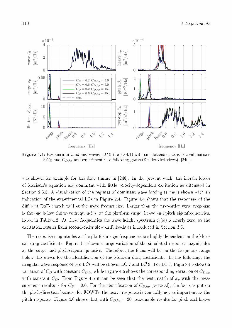
110 4 Experiments
CD = 0.2, CD,hp = 5.0
CD = 0.6, CD,hp = 5.0
CD = 0.2, CD,hp = 15.0
CD = 0.6, CD,hp = 15.0
exp.
frequency [Hz]
twr-
topxtt
[m2/s
2/H
z]
frequency [Hz]
lin.t
en.Fline1
[N2/H
z]
pit
chβp
[10−
3/H
z]
surg
exp
[m2/H
z]
hea
vez p
[m2/H
z]
wav
eζ 0
[m2/H
z]
surge
pitch
heav
e0.6
0.8
1.0
1.2
1.4
surge
pitch
heav
e0.6
0.8
1.0
1.2
1.4
×10−4×10−3
0
1
0
5
10
0
1
2
0
0.05
0
5
0
2
4
Figure 4.4: Response to wind and waves, LC 9 (Table 4.1) with simulations of various combinationsof CD and CD,hp and experiment (see following graphs for detailed views), [240].
was shown for example for the drag tuning in [248]. In the present work, the inertia forces
of Morison's equation are dominant with little velocity-dependent excitation as discussed in
Section 2.5.3. A visualization of the regimes of dominant wave forcing terms is shown with an
indication of the experimental LCs in Figure 2.4. Figure 4.4 shows that the responses of the
dierent DoFs match well at the wave frequencies. Larger than the rst-order wave response
is the one below the wave frequencies, at the platform surge, heave and pitch eigenfrequencies,
listed in Table 4.2. At these frequencies the wave height spectrum ζ0(ω) is nearly zero, so the
excitation results from second-order slow drift loads as introduced in Section 3.5.
The response magnitudes at the platform eigenfrequencies are highly dependent on the Mori-
son drag coecients: Figure 4.4 shows a large variation of the simulated response magnitudes
at the surge and pitch-eigenfrequencies. Therefore, the focus will be on the frequency range
below the waves for the identication of the Morison drag coecients. In the following, the
irregular wave response of two LCs will be shown, LC 7 and LC 9. For LC 7, Figure 4.5 shows a
variation of CD with constant CD,hp while Figure 4.6 shows the corresponding variation of CD,hpwith constant CD. From Figure 4.5 it can be seen that the best match of xp with the mea-
surement results is for CD = 0.6. For the identication of CD,hp (vertical), the focus is put on
the pitch-direction because for FOWTs, the heave response is generally not as important as the
pitch response. Figure 4.6 shows that with CD,hp = 20, reasonable results for pitch and heave
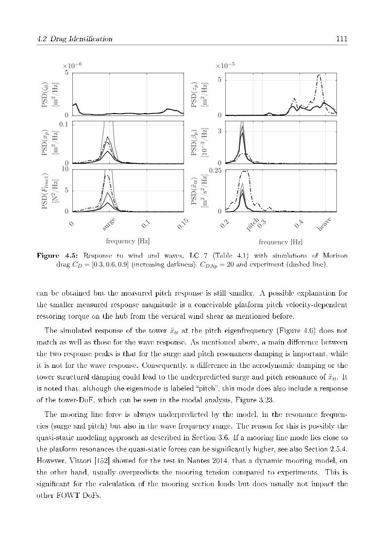
4.2 Drag Identication 111
frequency [Hz]
PSD
(xtt)
[m2/s
2/H
z]
frequency [Hz]
PSD
(Fline1
)
[N2/H
z]
PSD
(βp)
[10−
3/H
z]
PSD
(xp)
[m2/H
z]
PSD
(zp)
[m2/H
z]
PSD
(ζ0)
[m2/H
z]
0.2
pitch0.3
0.4
heav
e0
surge
0.1
0.15
×10−5×10−6
0
0.25
0
5
100
3
0
0.1
0
5
0
5
Figure 4.5: Response to wind and waves, LC 7 (Table 4.1) with simulations of Morisondrag CD = [0.3, 0.6, 0.9] (increasing darkness), CD,hp = 20 and experiment (dashed line).
can be obtained but the measured pitch response is still smaller. A possible explanation for
the smaller measured response magnitude is a conceivable platform pitch velocity-dependent
restoring torque on the hub from the vertical wind shear as mentioned before.
The simulated response of the tower xtt at the pitch eigenfrequency (Figure 4.6) does not
match as well as those for the wave response. As mentioned above, a main dierence between
the two response peaks is that for the surge and pitch resonances damping is important, while
it is not for the wave response. Consequently, a dierence in the aerodynamic damping or the
tower structural damping could lead to the underpredicted surge and pitch resonance of xtt. It
is noted that, although the eigenmode is labeled pitch, this mode does also include a response
of the tower-DoF, which can be seen in the modal analysis, Figure 3.23.
The mooring line force is always underpredicted by the model, in the resonance frequen-
cies (surge and pitch) but also in the wave frequency range. The reason for this is possibly the
quasi-static modeling approach as described in Section 3.6. If a mooring line mode lies close to
the platform resonances the quasi-static forces can be signicantly higher, see also Section 2.5.4.
However, Vittori [152] showed for the test in Nantes 2014, that a dynamic mooring model, on
the other hand, usually overpredicts the mooring tension compared to experiments. This is
signicant for the calculation of the mooring section loads but does usually not impact the
other FOWT DoFs.
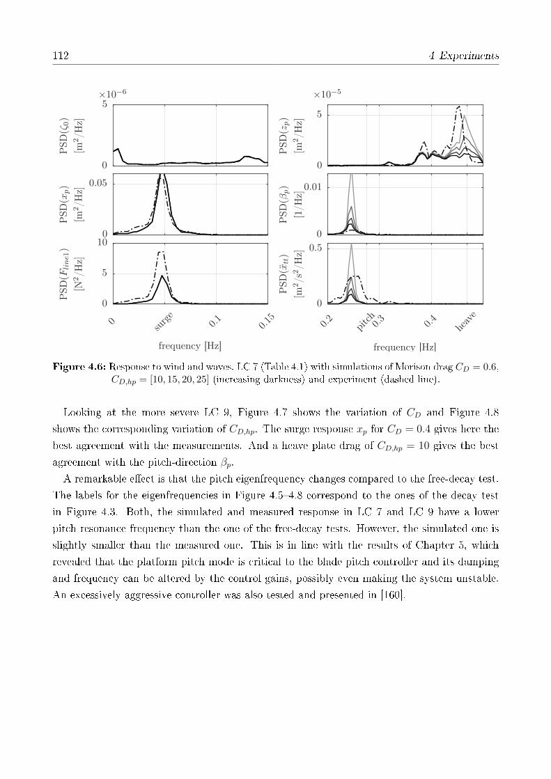
112 4 Experiments
frequency [Hz]
PSD
(xtt)
[m2/s
2/H
z]
frequency [Hz]
PSD
(Fline1
)
[N2/H
z]
PSD
(βp)
[1/H
z]
PSD
(xp)
[m2/H
z]
PSD
(zp)
[m2/H
z]
PSD
(ζ0)
[m2/H
z]
0.2
pitch0.3
0.4
heav
e0
surge
0.1
0.15
×10−5×10−6
0
0.5
0
5
100
0.01
0
0.05
0
5
0
5
Figure 4.6: Response to wind and waves, LC 7 (Table 4.1) with simulations of Morison drag CD = 0.6,CD,hp = [10, 15, 20, 25] (increasing darkness) and experiment (dashed line).
Looking at the more severe LC 9, Figure 4.7 shows the variation of CD and Figure 4.8
shows the corresponding variation of CD,hp. The surge response xp for CD = 0.4 gives here the
best agreement with the measurements. And a heave plate drag of CD,hp = 10 gives the best
agreement with the pitch-direction βp.
A remarkable eect is that the pitch eigenfrequency changes compared to the free-decay test.
The labels for the eigenfrequencies in Figure 4.54.8 correspond to the ones of the decay test
in Figure 4.3. Both, the simulated and measured response in LC 7 and LC 9 have a lower
pitch resonance frequency than the one of the free-decay tests. However, the simulated one is
slightly smaller than the measured one. This is in line with the results of Chapter 5, which
revealed that the platform pitch mode is critical to the blade pitch controller and its damping
and frequency can be altered by the control gains, possibly even making the system unstable.
An excessively aggressive controller was also tested and presented in [160].

4.2 Drag Identication 113
frequency [Hz]
twr-
topxtt
[m2/s
2/H
z]
frequency [Hz]
lin.t
en.Fline1
[N2/H
z]
pit
chβp
[10−
3/H
z]
surg
exp
[m2/H
z]
hea
vez p
[m2/H
z]
wav
eζ 0
[m2/H
z]
0.2
pitch0.3
0.4
heav
e0
surge
0.1
0.15
×10−4×10−6
0
0.4
0
5
10
0
2.5
0
0.1
0
3
0
5
Figure 4.7: Response to wind and waves, LC 9 (Table 4.1) with simulations of Morisondrag CD = [0.2, 0.4, 0.6] (increasing darkness), CD,hp = 10 and experiment (dashed line), [240].
frequency [Hz]
twr-
topxtt
[m2/s
2/H
z]
frequency [Hz]
lin.t
en.Fline1
[N2/H
z]
pit
chβp
[10−
3/H
z]
surg
exp
[m2/H
z]
hea
vez p
[m2/H
z]
wav
eζ 0
[m2/H
z]
0.2
pitch0.3
0.4
heav
e0
surge
0.1
0.15
×10−4×10−6
0
0.4
0
5
10
0
3
0
0.08
0
4
0
5
Figure 4.8: Response to wind and waves, LC 9 (Table 4.1) with simulations of Morison drag CD = 0.4,CD,hp = [5, 10, 15] (increasing darkness) and experiment (dashed line), [240].
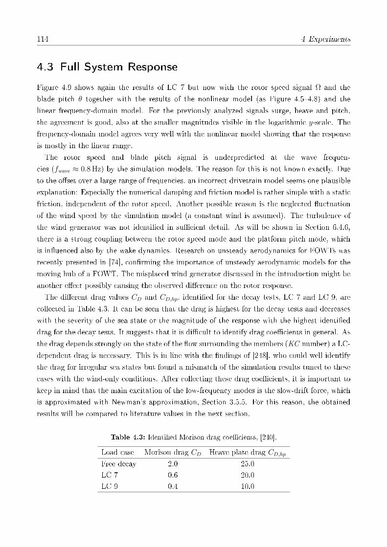
114 4 Experiments
4.3 Full System Response
Figure 4.9 shows again the results of LC 7 but now with the rotor speed signal Ω and the
blade pitch θ together with the results of the nonlinear model (as Figure 4.54.8) and the
linear frequency-domain model. For the previously analyzed signals surge, heave and pitch,
the agreement is good, also at the smaller magnitudes visible in the logarithmic y-scale. The
frequency-domain model agrees very well with the nonlinear model showing that the response
is mostly in the linear range.
The rotor speed and blade pitch signal is underpredicted at the wave frequen-
cies (fwave ≈ 0.8 Hz) by the simulation models. The reason for this is not known exactly. Due
to the oset over a large range of frequencies, an incorrect drivetrain model seems one plausible
explanation: Especially the numerical damping and friction model is rather simple with a static
friction, independent of the rotor speed. Another possible reason is the neglected uctuation
of the wind speed by the simulation model (a constant wind is assumed). The turbulence of
the wind generator was not identied in sucient detail. As will be shown in Section 6.4.6,
there is a strong coupling between the rotor speed mode and the platform pitch mode, which
is inuenced also by the wake dynamics. Research on unsteady aerodynamics for FOWTs was
recently presented in [74], conrming the importance of unsteady aerodynamic models for the
moving hub of a FOWT. The misplaced wind generator discussed in the introduction might be
another eect possibly causing the observed dierence on the rotor response.
The dierent drag values CD and CD,hp, identied for the decay tests, LC 7 and LC 9, are
collected in Table 4.3. It can be seen that the drag is highest for the decay tests and decreases
with the severity of the sea state or the magnitude of the response with the highest identied
drag for the decay tests. It suggests that it is dicult to identify drag coecients in general. As
the drag depends strongly on the state of the ow surrounding the members (KC number) a LC-
dependent drag is necessary. This is in line with the ndings of [248], who could well identify
the drag for irregular sea states but found a mismatch of the simulation results tuned to these
cases with the wind-only conditions. After collecting these drag coecients, it is important to
keep in mind that the main excitation of the low-frequency modes is the slow-drift force, which
is approximated with Newman's approximation, Section 3.5.5. For this reason, the obtained
results will be compared to literature values in the next section.
Table 4.3: Identied Morison drag coecients, [240].
Load case Morison drag CD Heave plate drag CD,hpFree decay 2.0 25.0LC 7 0.6 20.0LC 9 0.4 10.0
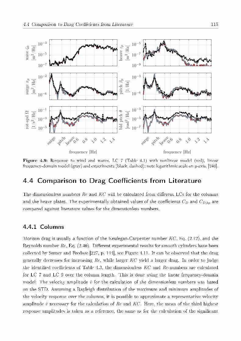
4.4 Comparison to Drag Coecients from Literature 115
frequency [Hz]
bld
ptc
hθ
[rad
2/H
z]
frequency [Hz]
rot-
spdΩ
[1/s
2/H
z]
pit
chβp
[1/H
z]
surg
exp
[m2/H
z]
hea
vez p
[m2/H
z]
wav
eζ 0
[m2/H
z]
surge
pitch
heav
e0.6
0.8
1.0
1.2
1.4
surge
pitch
heav
e0.6
0.8
1.0
1.2
1.4
10−7
10−5
10−3
10−5
10−3
10−1
10−6
10−3
10−6
10−2
10−9
10−7
10−5
10−7
10−5
10−3
Figure 4.9: Response to wind and waves, LC 7 (Table 4.1) with nonlinear model (red), linearfrequency-domain model (gray) and experiments (black, dashed); note logarithmic scale on y-axis, [240].
4.4 Comparison to Drag Coecients from Literature
The dimensionless numbers Re and KC will be calculated from dierent LCs for the columns
and the heave plates. The experimentally obtained values of the coecients CD and CD,hp are
compared against literature values for the dimensionless numbers.
4.4.1 Columns
Morison drag is usually a function of the Keulegan-Carpenter number KC , Eq. (2.12), and the
Reynolds number Re, Eq. (2.40). Dierent experimental results for smooth cylinders have been
collected by Sumer and Fredsøe [227, p. 144], see Figure 4.11. It can be observed that the drag
generally decreases for increasing Re, while larger KC yield a larger drag. In order to judge
the identied coecients of Table 4.3, the dimensionless KC and Re-numbers are calculated
for LC 7 and LC 9 over the column length. This is done using the linear frequency-domain
model: The velocity amplitude v for the calculation of the dimensionless numbers was based
on the STD. Assuming a Rayleigh distribution of the maximum and minimum amplitudes of
the velocity response over the columns, it is possible to approximate a representative velocity
amplitude v necessary for the calculation of Re and KC . Here, the mean of the third highest
response amplitudes is taken as a reference, the same as for the calculation of the signicant

116 4 Experiments
wave height Hs. The velocity v is calculated as
v ≈ kpeakσ(v), with kpeak = 2.0. (4.1)
Using the linear SLOW model, KC and Re are calculated once for the uid particle motion,
only and once for the body motion, only. The body motion is the one which inuences the
system damping, which in turn shows the largest sensitivity on the response-STD as shown in
the previous section. This is a major dierence to the validation of [248] because in that work
the Morison drag excitation forces (as opposed to damping forces) are of major importance.
Re×1e4 [-]KC [-]
body
mot
ion
dep
th[m
]
wav
em
otio
n
dep
th[m
]
0 1 2 3 4
0 5 10
0.2 0.4 0.6 0.8
0 0.5 1 1.5
-1
-0.6
-0.3
SWL
-1
-0.6
-0.3
SWL
Figure 4.10: Keulegan-Carpenter number and Reynolds number over depth from LC 7 (blue)and LC 9 (red) from linearized model.
The zero-upcrossing period T2 using the zeroth moment m0 (Eq.(2.28)) and the rst mo-
ment m1 of the respective spectrum (either from body motion or wave motion), is used for the
calculation of KC (Eq. (2.12)), see also [90, p. 5-42]
T2 = 2π
√m0
m1
. (4.2)
Figure 4.10 shows the Reynolds number and Keulegan-Carpenter number over the length of
a vertical column for both, LC 7 and LC 9 for the body motion and wave motion. It can be
seen that both, Re and KC increase with the sea state. Comparing the values to Figure 4.11,
it can be seen that the Keulegan-Carpenter number is KC < 1 and therefore out of the range
of Figure 4.11, while the Reynolds number Re ≈ 1× 10⁴ is at the lower end of the data. Such
low KC numbers suggest that the ow is even unseparated, see [115, p. 228]. Looking at the

4.4 Comparison to Drag Coecients from Literature 117
Figure 4.11: In-line force coecients for a free, smooth cylinder as function of the Re-number forvarious KC with vertical lines for Re-values corresponding to LC 7 (blue) and LC 9 (red). Adapted
from [227, p.144], reprinted with permission from author, 2018.
vertical axis of Fig 4.11 at Re = 1× 10⁴, the CD values decrease for decreasing KC and the
obtained values of Table 4.3 with CD = 0.4 (LC 9 and CD = 0.6 (LC 7) seem in a plausible
range.
Another, analytic equation for CD for circular cylinders of low KC is given by Wang in [115,
Eq. (7.21)]. It returns values of CD = 0.47 for LC 7 and CD = 0.2 for LC 9. The values are a
bit lower than the identied ones but the trend is the same and conrms the plausibility of the
experiments.
4.4.2 Heave plates
The same comparison can be made for the heave plates in vertical direction. Table 4.4 shows
the Reynolds number and Keulegan-Carpenter number for both LCs. Due to the low response
in heave-direction, the values are even smaller than for the columns. However, now the values
are within the range of the literature values taken from [230] and reprinted in Figure 4.12. The
data is compared in the publications for heave plates of dierent porosity, while here only the
black diamonds of zero porosity are of interest. For the body motion of the more severe LC 9,
we get KC = 0.35. Reading the corresponding CD,hp o Figure 4.12 results in CD,hp ≈ 10.
This is equal to the identied value for LC 9 of Table 4.3. For the mild sea state (LC 7),
one obtains KC = 0.054 with an identied CD,hp = 20. This value seems also plausible when
extrapolating the present data of Figure 4.12 to the left. The heave plate drag is independent
of the Reynolds number due to the sharp corners and small thickness of 3 mm.
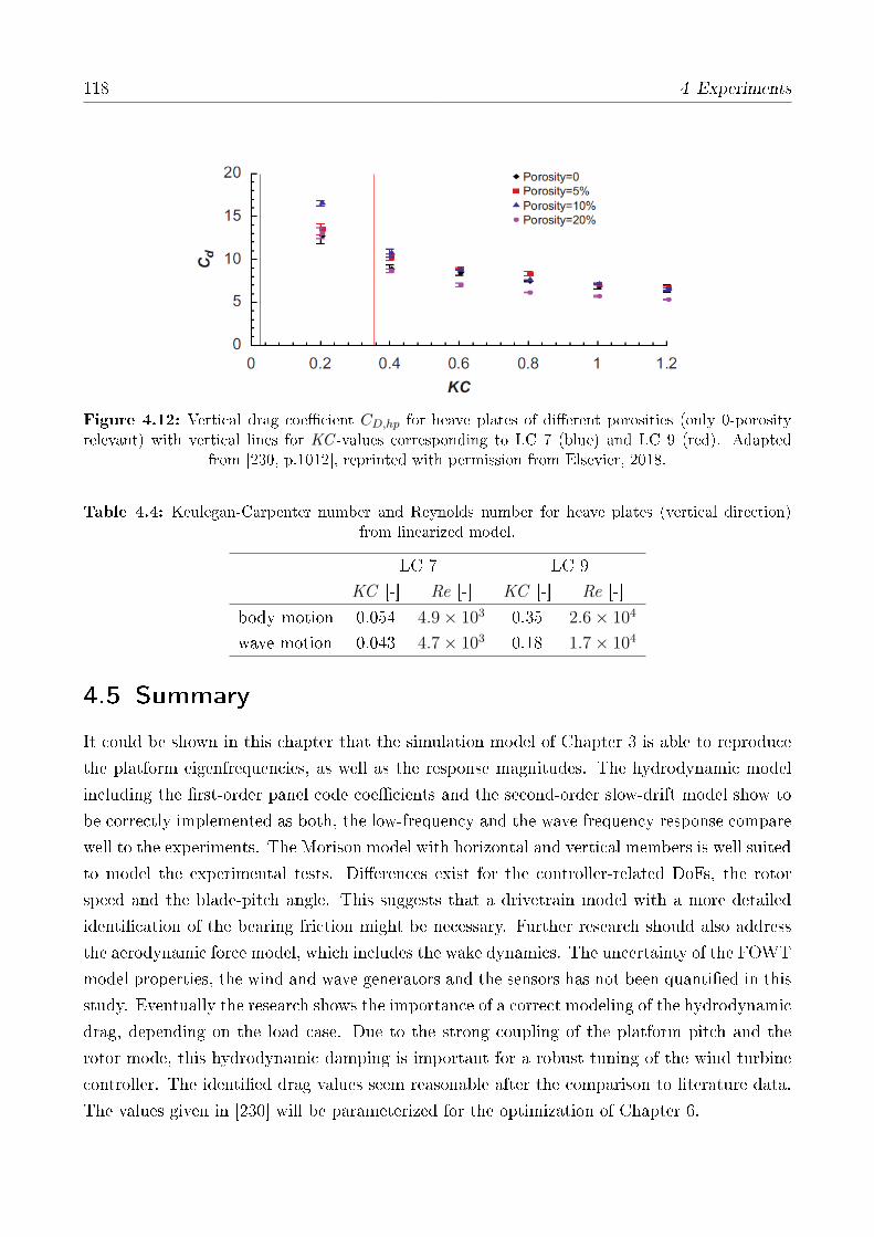
118 4 Experiments
Figure 4.12: Vertical drag coecient CD,hp for heave plates of dierent porosities (only 0-porosityrelevant) with vertical lines for KC -values corresponding to LC 7 (blue) and LC 9 (red). Adapted
from [230, p.1012], reprinted with permission from Elsevier, 2018.
Table 4.4: Keulegan-Carpenter number and Reynolds number for heave plates (vertical direction)from linearized model.
LC 7 LC 9KC [-] Re [-] KC [-] Re [-]
body motion 0.054 4.9× 10³ 0.35 2.6× 10⁴
wave motion 0.043 4.7× 10³ 0.18 1.7× 10⁴
4.5 Summary
It could be shown in this chapter that the simulation model of Chapter 3 is able to reproduce
the platform eigenfrequencies, as well as the response magnitudes. The hydrodynamic model
including the rst-order panel code coecients and the second-order slow-drift model show to
be correctly implemented as both, the low-frequency and the wave frequency response compare
well to the experiments. The Morison model with horizontal and vertical members is well suited
to model the experimental tests. Dierences exist for the controller-related DoFs, the rotor
speed and the blade-pitch angle. This suggests that a drivetrain model with a more detailed
identication of the bearing friction might be necessary. Further research should also address
the aerodynamic force model, which includes the wake dynamics. The uncertainty of the FOWT
model properties, the wind and wave generators and the sensors has not been quantied in this
study. Eventually the research shows the importance of a correct modeling of the hydrodynamic
drag, depending on the load case. Due to the strong coupling of the platform pitch and the
rotor mode, this hydrodynamic damping is important for a robust tuning of the wind turbine
controller. The identied drag values seem reasonable after the comparison to literature data.
The values given in [230] will be parameterized for the optimization of Chapter 6.
5 Controller Design
This chapter starts with a linear system analysis with the previously developed model to get an
understanding of the coupled properties of the dynamic FOWT system, relevant for controller
design. After the standard below-rated controller is introduced, a new scheme for a robust PI-
controller for above-rated conditions will be developed. It uses only the rotor speed error as
input and actuates the blade pitch angle (SISO) and relies therefore on a standard control
architecture. However, the gain scheduling is designed such that the system robustness is
ensured at all operating points. This criterion is the basis for a new, automated, model-based
design algorithm, in order to be used for the integrated optimization of Chapter 6. This gain
scheduling controller is subject of the paper [249].
Next to this SISO controller, an optimal MIMO controller will be designed for above-rated
conditions. It has the objective of showing the principally possible upper bound of the controller
performance, to be compared to the standard SISO controller. Thus, it is another reference
for the integrated optimization. The design is here done for the TripleSpar of Section 2.10 but
the validity of the controllers is ensured for the entire design space of platforms of Chapter 6.
This MIMO-controller and a linear system analysis as in the next section is subject of the
paper [205].
5.1 Linear System Analysis
In this section, an input-output scaling will be applied to the transfer function from disturbance
inputs d = [v0, ζ0]T (wind speed and wave height) and control inputs u = [Mg, θ]T (generator
torque and blade pitch angle) to the outputs y = [Ω, xt]T (rotor speed and tower-top displace-
ment from bending). This allows for a quantization and comparison of the eects of the dierent
system inputs. Next, the coupling of the system from the control inputs and disturbance inputs
to the outputs will be examined in a MIMO system analysis. The analyses are made with a
focus on the diculties arising from the RHPZ due to the oating platform, which is especially
critical slightly above rated. This is why the operating point is selected as v0 = 13 m/s.

120 5 Controller Design
5.1.1 Scaling
The scaling law to obtain the dimensionless system transfer function G from the dimensional
one G following [166] reads
G = D−1y GDu∗ . (5.1)
The scaling matrix for inputs Du∗ includes control and disturbance inputs u∗ = [u,d]T . For
the chosen input and output signals it results
Du∗ = diag([ Mg, θ, v0, ζ0 ]) and Dy = diag([ Ω, xt ]). (5.2)
The scaling factors are usually dened based on actuator constraints or maximum allowable
excursions, respectively, see [166]. Here, the specied requirements for the controller perfor-
mance of Table 2.2 were used for the rotor speed Ω and the generator torqueMg. For all others,
simulation results of the DTU 10 MW RWT on the TripleSpar at vhub = 13 m/s in closed-loop
were used with the sea states of Table 2.1. The scaling factors are based on the STD σ of
the respective signals. The 2σ values are used as in Section 4.4, which is the mean of the
third largest amplitudes for a narrow-banded process, see Section 2.7.3. All scaling factors are
collected in Table 5.1.
Table 5.1: Scaling factors.
u d y
Mg = 0.15Mg,rated = 31.1 kNm v0 = 2σ = 2.4 m/s Ω = 0.15 Ωrated = 1.44 rpm
θ = 2σ = 6.0 deg ζ0 = 2σ = 14Hs = 1.4 m xt = 2σ = 0.28 m
5.1.2 Input-output analysis
As discussed in Section 2.9, the biggest challenge for FOWT control is maintaining the rotor
speed while at the same time damping the platform motion. With the two standard actuators
of blade pitch θ and generator torque Mg, generally two control inputs are available and it
is also possible to feed back more signals than the rotor speed Ω. This encourages MIMO
controllers, which have the potential of mitigating the RHPZ [166]. In this section, the scaled
transfer dynamics from the control inputs u to the outputs y at a wind speed of v0 = 13 m/s
is analyzed. Figure 5.1 shows the 2 × 2 transfer function as Bode plots: At each frequency,
a sinusoidal input signal is amplied by the factor of the upper Bode plot. Additionally, the
amplied output is shifted by the phase angle of the lower Bode plot. Consequently, Figure 5.1
shows two properties: The transfer functions, including the poles and zeros, causing changes in
the phase, depending on their location in the complex plane (Figure 3.24) and additionally, the
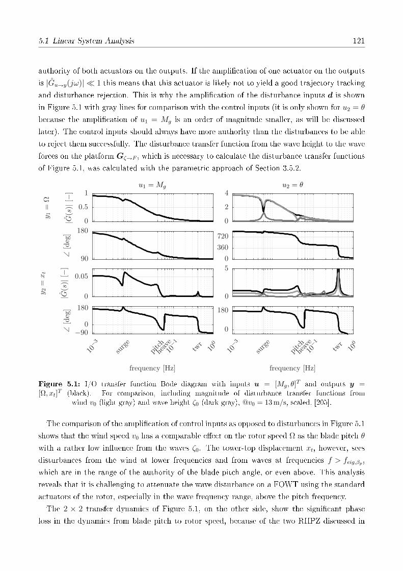
5.1 Linear System Analysis 121
authority of both actuators on the outputs. If the amplication of one actuator on the outputs
is |Guy(jω)| 1 this means that this actuator is likely not to yield a good trajectory tracking
and disturbance rejection. This is why the amplication of the disturbance inputs d is shown
in Figure 5.1 with gray lines for comparison with the control inputs (it is only shown for u2 = θ
because the amplication of u1 = Mg is an order of magnitude smaller, as will be discussed
later). The control inputs should always have more authority than the disturbances to be able
to reject them successfully. The disturbance transfer function from the wave height to the wave
forces on the platform GζF , which is necessary to calculate the disturbance transfer functions
of Figure 5.1, was calculated with the parametric approach of Section 3.5.2.
PSfrag replacements
u2 = θu1 = Mg
frequency [Hz]frequency [Hz]
∠[deg]
y 2=
xt
|G(s)|[−
]∠
[deg]
y 1=
Ω
|G(s)|[−
]
10−3
surge
pitch
heav
e
10−1
twr
100
10−3
surge
pitch
heav
e
10−1
twr
100
0
180
0
5
0
360
720
0
2
4
−900
180
0
0.05
90
180
0
0.5
1
Figure 5.1: I/O transfer function Bode diagram with inputs u = [Mg, θ]T and outputs y =
[Ω, xt]T (black). For comparison, including magnitude of disturbance transfer functions from
wind v0 (light gray) and wave height ζ0 (dark gray), @v0 = 13 m/s, scaled, [205].
The comparison of the amplication of control inputs as opposed to disturbances in Figure 5.1
shows that the wind speed v0 has a comparable eect on the rotor speed Ω as the blade pitch θ
with a rather low inuence from the waves ζ0. The tower-top displacement xt, however, sees
disturbances from the wind at lower frequencies and from waves at frequencies f > feig,βp ,
which are in the range of the authority of the blade pitch angle, or even above. This analysis
reveals that it is challenging to attenuate the wave disturbance on a FOWT using the standard
actuators of the rotor, especially in the wave frequency range, above the pitch frequency.
The 2 × 2 transfer dynamics of Figure 5.1, on the other side, show the signicant phase
loss in the dynamics from blade pitch to rotor speed, because of the two RHPZ discussed in
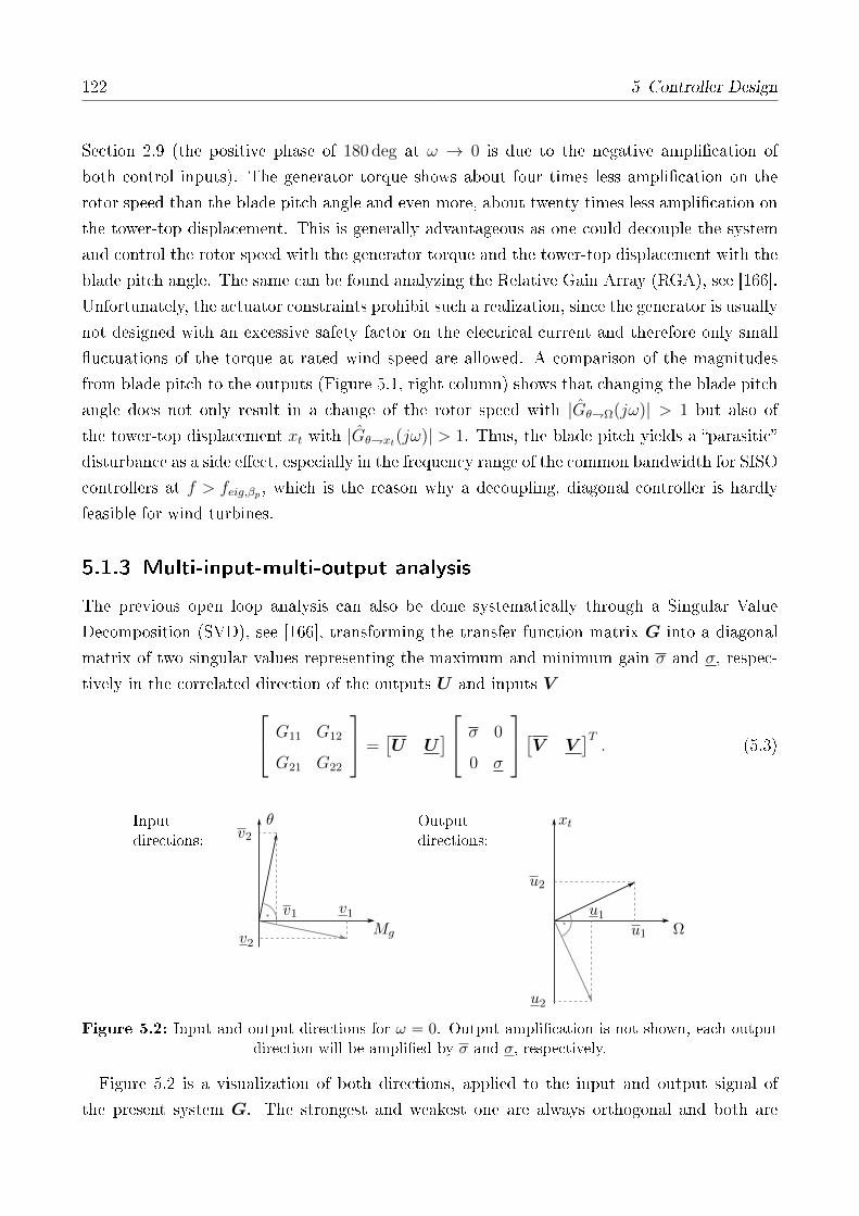
122 5 Controller Design
Section 2.9 (the positive phase of 180 deg at ω → 0 is due to the negative amplication of
both control inputs). The generator torque shows about four times less amplication on the
rotor speed than the blade pitch angle and even more, about twenty times less amplication on
the tower-top displacement. This is generally advantageous as one could decouple the system
and control the rotor speed with the generator torque and the tower-top displacement with the
blade pitch angle. The same can be found analyzing the Relative Gain Array (RGA), see [166].
Unfortunately, the actuator constraints prohibit such a realization, since the generator is usually
not designed with an excessive safety factor on the electrical current and therefore only small
uctuations of the torque at rated wind speed are allowed. A comparison of the magnitudes
from blade pitch to the outputs (Figure 5.1, right column) shows that changing the blade pitch
angle does not only result in a change of the rotor speed with |GθΩ(jω)| > 1 but also of
the tower-top displacement xt with |Gθxt(jω)| > 1. Thus, the blade pitch yields a parasitic
disturbance as a side eect, especially in the frequency range of the common bandwidth for SISO
controllers at f > feig,βp , which is the reason why a decoupling, diagonal controller is hardly
feasible for wind turbines.
5.1.3 Multi-input-multi-output analysis
The previous open loop analysis can also be done systematically through a Singular Value
Decomposition (SVD), see [166], transforming the transfer function matrix G into a diagonal
matrix of two singular values representing the maximum and minimum gain σ and σ, respec-
tively in the correlated direction of the outputs U and inputs V
G11 G12
G21 G22
=
[U U
] σ 0
0 σ
[V V
]T. (5.3)
Mg
θ
v1
v2
v2
v1
Ω
xt
u1
u2
u2
u1
Inputdirections:
Outputdirections:
Figure 5.2: Input and output directions for ω = 0. Output amplication is not shown, each outputdirection will be amplied by σ and σ, respectively.
Figure 5.2 is a visualization of both directions, applied to the input and output signal of
the present system G. The strongest and weakest one are always orthogonal and both are

5.1 Linear System Analysis 123
PSfrag replacements
MIMO
zero
MIMO
zero
frequency [Hz]
gain
σ[−
]
1st
coor
d.
(Ω)
ofou
tput
dir
.
1st
coor
d.(M
g)
ofin
put
dir
.
10−3
surge
pitch
heav
e
10−1
twr
100
0
5
10
0
0.5
1
0
0.5
1
Figure 5.3: Singular-value decomposition of I/O transfer function: Strongest (dark) and weak-est (light) input and output directions with associated gains: The rst plot shows the rst coordinateof the input coordinates u = [Mg, θ]
T and the second plot the rst coordinate of the output coordinatesy = [Ω, xt]
T , the third plot shows the gain associated with the strongest and weakest direction andthe MIMO zeros of G, @v0 = 13 m/s, [205].
amplied individually by σ and σ, respectively. Figure 5.2 visualizes the zero-frequency limit
of the frequency-dependent SVD of Figure 5.3. We can now investigate the combination of
the inputs that yield the highest gain on the outputs. This strongest gain σ is associated
with the strongest output direction. Thus, this analysis addresses the true MIMO system with
combinations of the inputs and their eect on the outputs, as opposed to Figure 5.1, which
shows the independent transfer dynamics.
Figure 5.3 shows in the upper two graphs the rst coordinate of the input and output di-
rections (abscissa of Figure 5.2). It can be seen that the strongest singular value in dark color
contains only little contribution of the generator torque Mg but a high portion of the blade
pitch angle θ, which conrms the ndings from the I/O transfer function matrix of Figure 5.1.
Looking at frequencies up to the platform pitch eigenfrequency this combination of inputs (or
direction) is well suited to control the rotor speed Ω (second plot, dark color). At the platform
pitch eigenfrequency, the strongest gain σ decreases, showing that the control of both, the rotor
speed and the tower becomes rather dicult.
One can assess the eect of using the two control inputs (Mg, θ) as compared to the blade
pitch angle, only: The strongest singular value yields slightly higher gains (Figure 5.3, bottom)
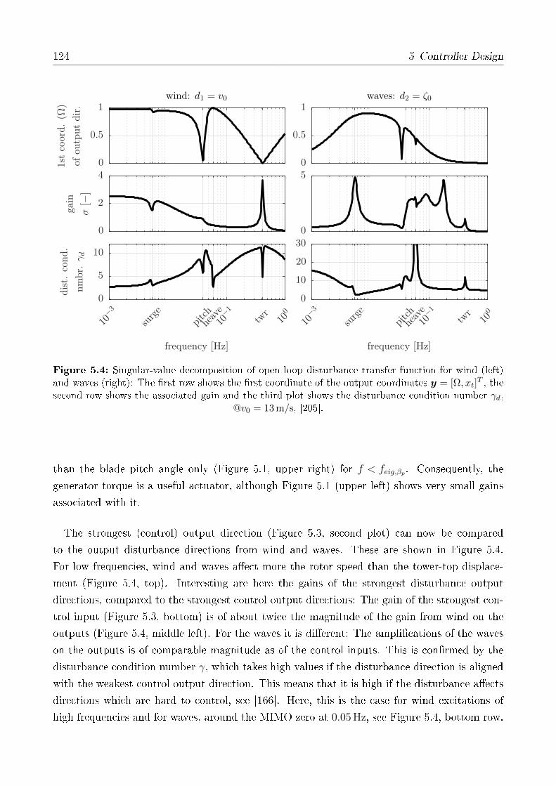
124 5 Controller Design
PSfrag replacements
waves: d2 = ζ0wind: d1 = v0
frequency [Hz]frequency [Hz]
dis
t.co
nd.
nm
br.
γd
gain
σ[−
]
1st
coor
d.
(Ω)
ofou
tput
dir
.
10−3
surge
pitchhe
ave
10−1
twr
100
10−3
surge
pitchhe
ave
10−1
twr
100
0
10
20
300
50
0.5
1
0
5
10
0
2
40
0.5
1
Figure 5.4: Singular-value decomposition of open loop disturbance transfer function for wind (left)and waves (right): The rst row shows the rst coordinate of the output coordinates y = [Ω, xt]
T , thesecond row shows the associated gain and the third plot shows the disturbance condition number γd,
@v0 = 13 m/s, [205].
than the blade pitch angle only (Figure 5.1, upper right) for f < feig,βp . Consequently, the
generator torque is a useful actuator, although Figure 5.1 (upper left) shows very small gains
associated with it.
The strongest (control) output direction (Figure 5.3, second plot) can now be compared
to the output disturbance directions from wind and waves. These are shown in Figure 5.4.
For low frequencies, wind and waves aect more the rotor speed than the tower-top displace-
ment (Figure 5.4, top). Interesting are here the gains of the strongest disturbance output
directions, compared to the strongest control output directions: The gain of the strongest con-
trol input (Figure 5.3, bottom) is of about twice the magnitude of the gain from wind on the
outputs (Figure 5.4, middle left). For the waves it is dierent: The amplications of the waves
on the outputs is of comparable magnitude as of the control inputs. This is conrmed by the
disturbance condition number γ, which takes high values if the disturbance direction is aligned
with the weakest control output direction. This means that it is high if the disturbance aects
directions which are hard to control, see [166]. Here, this is the case for wind excitations of
high frequencies and for waves, around the MIMO zero at 0.05 Hz, see Figure 5.4, bottom row.

5.2 Below-Rated Controller 125
5.1.4 Summary
The main ndings of the OL analysis are rst, the dierent impact of the two actuators blade
pitch and generator torque on the rotor speed. The amplication of the blade pitch signal on the
rotor speed proves its better suitability for control, compared to the generator torque. However,
blade pitch has, as opposed to the generator torque, the negative side eect that it inuences
more the tower-top fore-aft forcing than does the generator torque. This nding inuences the
selection of a MIMO control layout: While it would be desirable to have two control inputs
with two dierent controlled variables with no interaction of one loop on the other, this seems
not possible due to the generator torque constraints. Second, it was shown that supporting
rotor-speed control with a slight portion of generator torque actuation can improve the control
performance while exciting less the tower-top motion. However, the control against the wave
forcing is found to be challenging, especially at the frequencies of common wave spectra.
5.2 Below-Rated Controller
For wind speeds between cut-in (4 m/s) and rated wind (11.4 m/s), a standard KΩ2-controller
is used for both of the above-rated controllers to be designed in the next sections. The below-
rated controller will not be adjusted to the dierent platform designs in this work because it
does not inuence the system stability as the above-rated controller. The goal is to control the
rotor speed for optimal power production at TSR λ = ΩR/v0 = λopt, see Section 2.9. Therefore,
the generator torque Mg is a nonlinear state feedback of the rotor speed Ω following [44] as
Mg = kΩΩ2g with kΩ =
1
2ρaπR
3 cp,maxλopt
. (5.4)
For the DTU 10 MW RWT, the rated generator torque is rather low compared to the rotor
properties. Therefore, there is no increase of generator torque necessary in the transition from
the optimal-TSR region and the above-rated region. Often, the switching methodology to the
above-rated control region substantially inuences the overall fatigue loads of the rotor and
the tower. In this work, this switching is not a focus but rather the design of the above-rated
controller. The tested wind speeds of Chapter 6 yield only few switching events.
5.3 Robust Proportional-Integral Controller
As described in Section 2.9, a common way of designing SISO controllers for FOWTs is to de-
tune the gains, making the controller less aggressive to avoid instability due to the RHPZ.
A common method, described in [10] and [15], and repeatedly used for the generic FOWT
concepts OC3 and OC4, see [111, 112], is to model the de-coupled (rigid) rotor including

126 5 Controller Design
Ωref /igear+
θ
v0
G(s)
kp(θ)
1Ti
1s
Ωg
+
+
Figure 5.5: PI-controller for above-rated wind speeds.
aerodynamics and design the controller such that the closed-loop-eigenfrequency of the rotor
lies below the fundamental platform eigenfrequency (usually platform pitch, see Section 2.5). As
discussed already in Section 2.9, this method gives good rst guesses for reasonable control gains
without large modeling eorts (the oater and tower dynamics do not have to be represented).
However, mainly the gain scheduling law does not always yield reasonable results. It suggests
constant dynamics over the entire operating range, which is the intention of gain scheduling.
But this is not always true because of the neglected fore-aft dynamics in the model. With a
more rened simulation model, the rotor dynamics in closed-loop will alter signicantly over
the operating range, contradicting the design conditions.
Here, a method is proposed based on the linearized model of Chapter 3, which includes the
oater dynamics, especially the platform pitch mode. For a robust PI-controller, stability is the
rst criterion and the rotor eigendynamics (as in the above de-tuning method) is a secondary
criterion. Thus, the controller ensures a certain robustness over the operating range, which is
important considering the RHPZ and also the uncertainty related to the system damping, see
Chapter 4.
Figure 5.5 shows the block diagram of the controller. There is no explicit gain scheduling
factor included. Instead, the proportional gain is written as a function of the blade pitch
angle kp = kp(θ). The controller maintains a constant generator torque Mg in the above-rated
wind speed region. The feedback control law reads with the azimuth angle ϕ =∫
Ω dt, equal
to the integral of the rotor speed Ω, the PI time constant Ti and the gear ratio igear
∆θ =kp(θ)
igear∆Ω +
kp(θ)
igearTi∆ϕ. (5.5)
Using the Nyquist criterion, see [166], a Gain Margin (GM) and a Phase Margin (PM) can
be dened as a design criterion. Here, a dierent method is chosen, involving only a single
criterion, in order to simplify the automation intended for this controller. The single criterion is
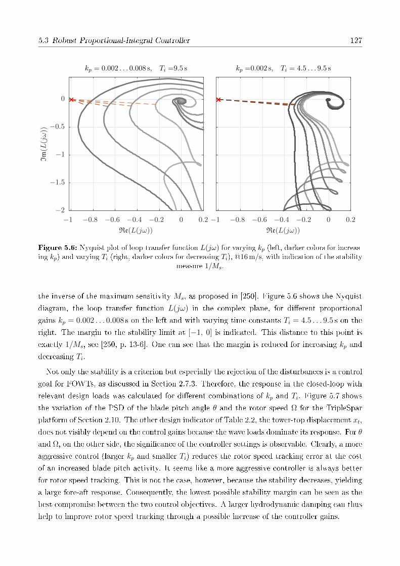
5.3 Robust Proportional-Integral Controller 127
PSfrag replacements
kp =0.002 s, Ti = 4.5 . . . 9.5 skp = 0.002 . . . 0.008 s, Ti =9.5 s
Re(L(jω))Re(L(jω))
Im(L
(jω))
−1 −0.8 −0.6 −0.4 −0.2 0 0.2−1 −0.8 −0.6 −0.4 −0.2 0 0.2
−2
−1.5
−1
−0.5
0
Figure 5.6: Nyquist plot of loop-transfer function L(jω) for varying kp (left, darker colors for increas-ing kp) and varying Ti (right, darker colors for decreasing Ti), @16 m/s, with indication of the stability
measure 1/Ms.
the inverse of the maximum sensitivity Ms, as proposed in [250]. Figure 5.6 shows the Nyquist
diagram, the loop transfer function L(jω) in the complex plane, for dierent proportional
gains kp = 0.002 . . . 0.008 s on the left and with varying time constants Ti = 4.5 . . . 9.5 s on the
right. The margin to the stability limit at [−1, 0] is indicated. This distance to this point is
exactly 1/Ms, see [250, p. 13-6]. One can see that the margin is reduced for increasing kp and
decreasing Ti.
Not only the stability is a criterion but especially the rejection of the disturbances is a control
goal for FOWTs, as discussed in Section 2.7.3. Therefore, the response in the closed-loop with
relevant design loads was calculated for dierent combinations of kp and Ti. Figure 5.7 shows
the variation of the PSD of the blade pitch angle θ and the rotor speed Ω for the TripleSpar
platform of Section 2.10. The other design indicator of Table 2.2, the tower-top displacement xt,
does not visibly depend on the control gains because the wave loads dominate its response. For θ
and Ω, on the other side, the signicance of the controller settings is observable. Clearly, a more
aggressive control (larger kp and smaller Ti) reduces the rotor speed tracking error at the cost
of an increased blade pitch activity. It seems like a more aggressive controller is always better
for rotor speed tracking. This is not the case, however, because the stability decreases, yielding
a large fore-aft response. Consequently, the lowest possible stability margin can be seen as the
best compromise between the two control objectives. A larger hydrodynamic damping can thus
help to improve rotor speed tracking through a possible increase of the controller gains.

128 5 Controller Design
frequency [Hz]frequency [Hz]
PSD
Ω[rad
2/s
2/H
z]P
SD
θ[rad
2/H
z]
10−3
surge
pitchhe
ave
10−1
10−3
surge
pitchhe
ave
10−1
0
0.2
0.4
0.60
0.05
0.1
Figure 5.7: PSDs of rotor speed Ω and blade pitch angle θ for kp = 0.002 . . . 0.008 s withTi = 9.5 s (left) and Ti = 4.5 . . . 9.5 s with kp = 0.002 (right), darker colors for more aggressive gains
(larger kp, smaller Ti) @16 m/s.
In a next step, the criteria for setting up a gain scheduling law over wind speeds are set up.
The rst design criterion is the stability margin of 1/Ms = 0.4. The corresponding gains kp can
be interpolated after calculating the margins 1/Ms for a grid of wind speeds v0, gains kp and
time constants Ti. Figure 5.8 shows dierent quantities, all interpolated at the stability limit
of 1/Ms = 0.4 for dierent Ti. The rst is the proportional gain kp, which decreases initially
before it raises again at higher wind speeds. On the right-hand side of Figure 5.8, the STD
of the rotor speed Ω, the blade pitch angle θ and the tower-top displacement xt can be seen.
For all signals the largest Ti yield the smallest uctuations. This might be connected with
the observation that larger Ti yield a higher damping of the rotor-speed mode (see pole-zero
map, Figure 3.24). The properties of the rotor mode can be seen in the two plots on the
lower left of Figure 5.8. The pole magnitude λrot is equal to the undamped eigenfrequency for
undercritically damped poles with ξrot < 1. For overcritically damped poles, only the magnitude
of the dominant, smaller pole is shown, which is equal to the inverse of the time constant τrot,
see Figure 3.24b. With higher wind speeds and increasing Ti, the rotor dynamics become faster
and the damping ratio increases up to the overcritical range.
Following the observations of Figure 5.8, the time constant was xed to Ti = 9.5 s, a value
up to which the performance increases slowly with no improvements beyond. For higher wind
speeds, stability is not an issue because for v0 > 20 m/s, the limit of 1/Ms = 0.4 cannot
be reached anymore for the investigated range of gains kp, see Figure 5.8. Therefore, the

5.3 Robust Proportional-Integral Controller 129
PSfrag replacements
v0 [m/s]
STD(x
t)[m
]STD(θ)
[rad
]STD(Ω
)[r
ad/s
]
v0 [m/s]
ξ rot[-]
|λrot|[
1/s]
kp
[s]
12 14 16 18 2012 14 16 18 20
0.12
0.14
0.16
0.18
0.02
0.04
0.06
0.08
0.05
0.1
0.5
1
0.05
0.1
0.15
0.2
0.3
0.4
Figure 5.8: Interpolated CL properties at the stability limit (1/Ms = 0.4) over wind speeds v0
for Ti = 4.5 . . . 9.5 s (increasing darkness).
time constant of the (overdamped) rotor mode is xed, as a secondary design criterion for
the gain scheduling. This is in line with the procedure of [10] but here it is calculated for
the coupled model instead of the rotor-only model. An algorithm identifying the eigenvectors
and assigning them to the states has been implemented for the automated design algorithm.
With this it is possible to interpolate the gains kp (with a constant Ti again) at the desired
eigenfrequency ω0,rot, or the desired time constant τrot for an overdamped mode.
Figure 5.9 shows the resulting gain scheduling kp = kp(v0) at the desired stability 1/Ms = 0.4
or the desired rotor closed-loop time constant τrot, respectively. It can be seen that the stability
requirement results in decreasing kp for wind speeds above rated. Towards the cut-out wind
speed of v0 = 25 m/s the stability criterion is not relevant anymore and the gain scheduling
takes the values which yield a constant τrot. At rated wind, the stability is most critical and
therefore the proposed criteria yield small kp. The design of the PI-controller needs to be
aligned with the switching procedure to below-rated winds.
The gain margins and phase margins for the gains at 1/Ms = 0.4 of Figure 5.9 are shown
in Figure 5.10. Recommended margins from control engineering textbooks are in the range
of GM ≈ 6 dB and PM = 40 . . . 60 deg. The resulting margins of the designed controller are
roughly in this range and slightly below for the gain margin at low wind speeds and the phase
margin at high wind speeds. This conrms that the chosen value of 1/Ms = 0.4 is reasonable.

130 5 Controller Design
kpτrot = 13.9 s1/Ms = 0.4
v0 [m/s]
kp
[s]
12 14 16 18 20 22 24
0
0.005
0.01
Figure 5.9: Gain scheduling of kp for Ti = 9.5 s obeying the stability limit of 1/Ms = 0.4 and targetinga CL rotor time constant of τrot = 13.3 s. Gain on high-speed shaft angular velocity is shown.
PSfrag replacements
v0 [m/s]
PM
[deg
]
v0 [m/s]
GM
[dB
]
12 14 16 18 2012 14 16 18 20
30
40
50
60
4
6
8
Figure 5.10: Gain margin and phase margin at 1/Ms = 0.4 over wind speeds.
PSfrag replacements
v0 [m/s]
Ω[%
]STD(θ)
[rad
]
v0 [m/s]
STD(x
t)[m
]STD(Ω
)[r
ad/s
]
12 14 16 18 20 22 24 2512 14 16 18 20 22 24 25
15
30
45
0
0.05
0.1
0.1
0.2
0.30
0.1
0.2
Figure 5.11: Simulation results for PI-controller with linearized model (blue), nonlinear model (red)and FAST (green) for load case of Table 2.1.
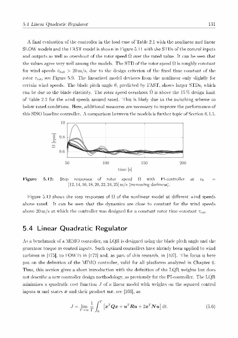
5.4 Linear Quadratic Regulator 131
A nal evaluation of the controller in the load case of Table 2.1 with the nonlinear and linear
SLOW models and the FAST model is shown in Figure 5.11 with the STDs of the control inputs
and outputs as well as overshoot of the rotor speed Ω over the rated value. It can be seen that
the values agree very well among the models. The STD of the rotor speed Ω is roughly constant
for wind speeds vhub > 20 m/s, due to the design criterion of the xed time constant of the
rotor τrot, see Figure 5.9. The linearized model deviates from the nonlinear only slightly for
certain wind speeds. The blade pitch angle θ, predicted by FAST, shows larger STDs, which
can be due to the blade elasticity. The rotor speed overshoot Ω is above the 15 % design limit
of Table 2.2 for the wind speeds around rated. This is likely due to the switching scheme to
below rated conditions. Here, additional measures are necessary to improve the performance of
this SISO baseline controller. A comparison between the models is further topic of Section 6.4.5.
PSfrag replacements
time [s]
Ω[r
pm
]
50 100 150 200
9.6
9.8
10
Figure 5.12: Step responses of rotor speed Ω with PI-controller at v0 =[12, 14, 16, 18, 20, 22, 24, 25] m/s (increasing darkness).
Figure 5.12 shows the step responses of Ω of the nonlinear model at dierent wind speeds
above rated. It can be seen that the dynamics are close to constant for the wind speeds
above 20 m/s at which the controller was designed for a constant rotor time constant τrot.
5.4 Linear Quadratic Regulator
As a benchmark of a MIMO controller, an LQR is designed using the blade pitch angle and the
generator torque as control inputs. Such optimal controllers have already been applied to wind
turbines in [175], to FOWTs in [172] and, as part of this research, in [107]. The focus is here
put on the denition of the MIMO controller, valid for all platforms analyzed in Chapter 6.
Thus, this section gives a short introduction with the denition of the LQR weights but does
not describe a new controller design methodology, as previously for the PI-controller. The LQR
minimizes a quadratic cost function J of a linear model with weights on the squared control
inputs u and states x and their product ux, see [166], as
J = limT→∞
1
T
∫ T
0
[xTQx+ uTRu+ 2xTNu
]dt. (5.6)
132 5 Controller Design
The weights R on the inputs u take the form
R = diag([rMg , rθ
])(5.7)
and for the weights on the states x only four nonzero weights are chosen as
Q = diag([
0, 0, 0, qϕ, 0, 0, 0, 0, qβp , qΩ, 0, qxt]). (5.8)
The order of the states follows Eq. (3.18) with the exible tower-DoF last. The weight on the
product of states and outputs is selected as
N(10, 1) = nΩ,Mg , N ∈ R(2f×nu). (5.9)
It has the purpose of reducing the power uctuation, which is the product of the tenth state Ω
and the rst control input Mg. The weighting factors inside R, Q, and N are shown in
Table 5.2. They are mostly normalized with the square of the scaling values of Table 5.1.
Although Table 5.1 is given for only one wind speed (v0 = 13 m/s), the response of most states
and inputs is highest around rated and therefore these weights are taken as a representative
reference for the entire operating range. In order to calculate amplitudes of the derivatives and
integrals of the scaling values of Table 5.1, a reference frequency of ω = 0.63 rad/s (= 0.1 Hz)
was chosen, the frequency of common wave spectra. The 2σ-value of the platform pitch angle βp,
not included in Table 5.1, is βp = 2.2 deg.
Table 5.2: LQR weights.
R Q N
rMg = 0.01
M2g
qϕ = 5.7× 10⁻⁴
(Ω/ω)2nΩ,Mg = 31.6
(ΩMg)2
rθ = 1.4× 10⁻³
θ2qΩ = 0.027
Ω2
qβp = 0.038
(βpω)2
qxt = 9.8× 10⁻⁶
(xtω)2
The solution of the Riccati equation [166] results in the state feedback matrix K lqr and the
feedback law of the LQR reads
u(t) = −K lqrx(t). (5.10)
An equivalent integral action for the rotor speed signal is included because the rotor az-
imuth ϕ = x(4) is part of the state vector x. Usually, the state signals, as inputs to the LQR,
need to be calculated by an observer. In this work, however, the states are assumed to be
perfectly measurable in order obtain a benchmark of an optimal control performance.
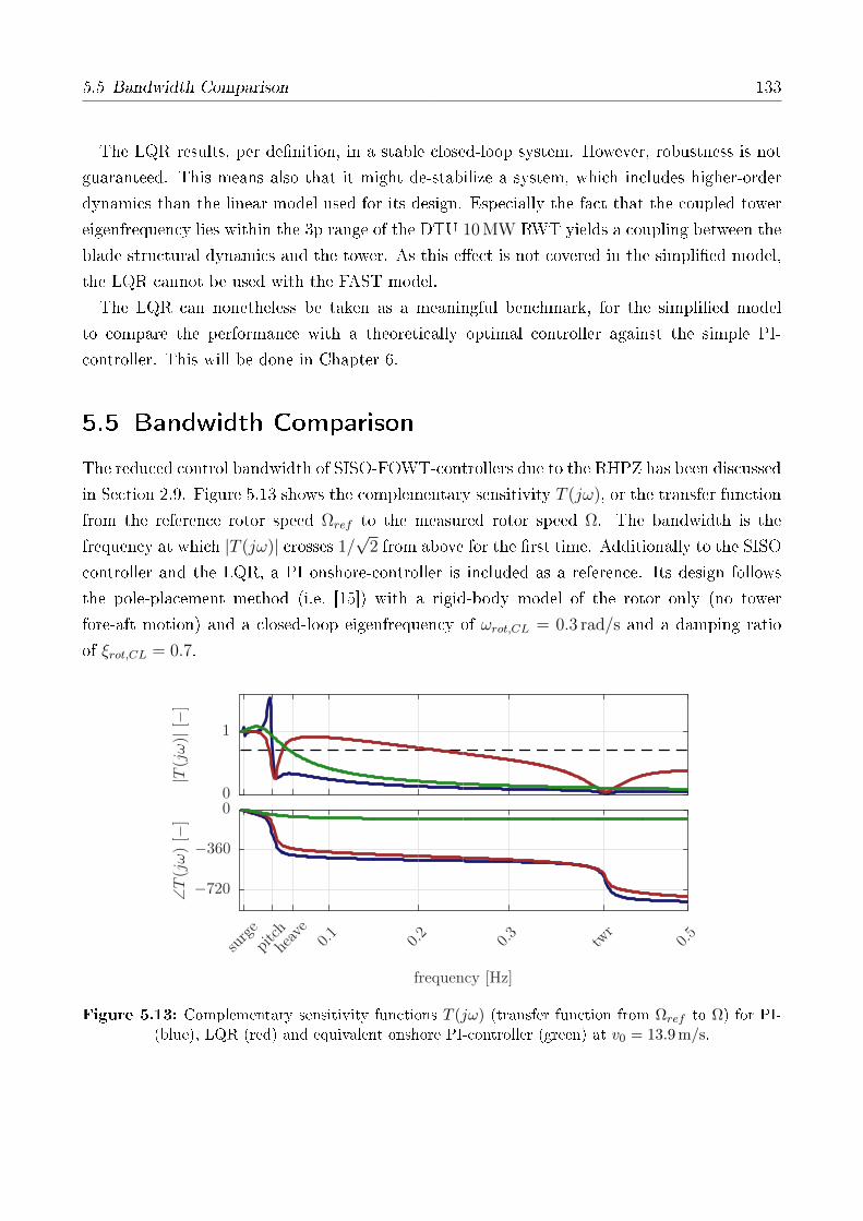
5.5 Bandwidth Comparison 133
The LQR results, per denition, in a stable closed-loop system. However, robustness is not
guaranteed. This means also that it might de-stabilize a system, which includes higher-order
dynamics than the linear model used for its design. Especially the fact that the coupled tower
eigenfrequency lies within the 3p range of the DTU 10 MW RWT yields a coupling between the
blade structural dynamics and the tower. As this eect is not covered in the simplied model,
the LQR cannot be used with the FAST model.
The LQR can nonetheless be taken as a meaningful benchmark, for the simplied model
to compare the performance with a theoretically optimal controller against the simple PI-
controller. This will be done in Chapter 6.
5.5 Bandwidth Comparison
The reduced control bandwidth of SISO-FOWT-controllers due to the RHPZ has been discussed
in Section 2.9. Figure 5.13 shows the complementary sensitivity T (jω), or the transfer function
from the reference rotor speed Ωref to the measured rotor speed Ω. The bandwidth is the
frequency at which |T (jω)| crosses 1/√
2 from above for the rst time. Additionally to the SISO
controller and the LQR, a PI onshore-controller is included as a reference. Its design follows
the pole-placement method (i.e. [15]) with a rigid-body model of the rotor only (no tower
fore-aft motion) and a closed-loop eigenfrequency of ωrot,CL = 0.3 rad/s and a damping ratio
of ξrot,CL = 0.7.
frequency [Hz]
∠T(jω)[−
]|T
(jω)|[−
]
surge
pitch
heav
e0.1
0.2
0.3
twr
0.5
−720
−360
00
1
Figure 5.13: Complementary sensitivity functions T (jω) (transfer function from Ωref to Ω) for PI-(blue), LQR (red) and equivalent onshore PI-controller (green) at v0 = 13.9 m/s.

134 5 Controller Design
For the two FOWT systems, the zero at the platform pitch eigenfrequency is well visible.
It is usually this mode which limits the bandwidth for semi-submersibles. The surge-mode
(lower frequency than pitch) has a higher damping and the other fore-aft mode, the tower, is
of a higher frequency. The onshore system, which does not have the soft fore-aft dynamics,
has an about 50 % larger bandwidth. Even though the LQR is a MIMO controller, feeding
back all states, the platform pitch mode is, also here, a limiter of the bandwidth. However,
it can be shown that a higher fore-aft damping or a shift of the RHPZ to the left-half plane
through more generator torque actuation can increase the bandwidth of the LQR. Such a case
was presented in [205], giving a bandwidth comparable to the onshore system through a smaller
weight on the generator torque Mg. This would, however, exceed the limits of Table 2.2. The
benets of the LQR are in this work still clearly visible in the results of Chapter 6, especially in
Figure 6.12, with an improved attenuation of the resonances and the low-frequency excitations
from wind and slow-drift forces.

6 Integrated Optimization
The numerical model of Chapter 3 and the parametric controllers of Chapter 5 will be used in
this chapter for an integrated design study. The parametric simulation model, including the pre-
processing for the hydrodynamics, allows for a calculation of the response of the coupled system
over a design space of oating platform geometries with an individually designed controller.
This is seen as a rst step towards Systems Engineering of FOWTs, as discussed in Section 2.4.
The inherent dynamic properties and the transmission of environmental loads on the structure
will be analyzed for the entire design space. The advantages of certain designs over others and
the underlying physics causing these dierences will be assessed in detail.
The structure of the chapter is such that the optimization methodology, the design space and
the parametric design approaches are introduced before various simulation results are shown:
Linear system analyses and operational fatigue loads and eventually design indicators for a
cascading of the obtained knowledge on optimal designs into feasible design criteria. The
chapter terminates with a verication of the results obtained from the reduced-order model
with the reference model FAST and further studies on the necessary model delity.
6.1 Methodology
The integrated optimization of this chapter has the objective of a sensitivity study, or brute-
force optimization rather than a closed-loop optimization. This has the reason that the focus
is not on a distinct optimization algorithm but on the understanding of the FOWT dynamics.
The parametric studies allow a clear visualization of the results such as structural loads, but
also system properties such as eigenfrequencies, damping ratios and transfer functions. A
closed-loop optimization was also done in the course of this thesis for the project LIFES50+,
see Deliverable 4.3 [251] and the associated conference paper [237]. The present approach is
subject of the publication [252].
Of major importance to the analysis is a reasonable denition of the design space and a clear
description of the problem to be answered: As was shown in Chapter 5, the rst-order wave
loads are of signicant magnitude and hardly controllable with the wind turbine actuators. It
was also shown that the platform pitch-direction has signicant eects on the wind turbine
operation as the platform pitch mode is a limiter to the controller bandwidth. Consequently,
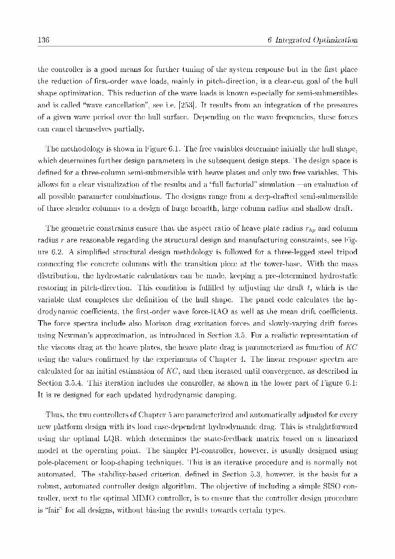
136 6 Integrated Optimization
the controller is a good means for further tuning of the system response but in the rst place
the reduction of rst-order wave loads, mainly in pitch-direction, is a clear-cut goal of the hull
shape optimization. This reduction of the wave loads is known especially for semi-submersibles
and is called wave cancellation, see i.e. [253]. It results from an integration of the pressures
of a given wave period over the hull surface. Depending on the wave frequencies, these forces
can cancel themselves partially.
The methodology is shown in Figure 6.1. The free variables determine initially the hull shape,
which determines further design parameters in the subsequent design steps. The design space is
dened for a three-column semi-submersible with heave plates and only two free variables. This
allows for a clear visualization of the results and a full factorial simulation an evaluation of
all possible parameter combinations. The designs range from a deep-drafted semi-submersible
of three slender columns to a design of large breadth, large column radius and shallow draft.
The geometric constraints ensure that the aspect ratio of heave plate radius rhp and column
radius r are reasonable regarding the structural design and manufacturing constraints, see Fig-
ure 6.2. A simplied structural design methdology is followed for a three-legged steel tripod
connecting the concrete columns with the transition piece at the tower-base. With the mass
distribution, the hydrostatic calculations can be made, keeping a pre-determined hydrostatic
restoring in pitch-direction. This condition is fullled by adjusting the draft t, which is the
variable that completes the denition of the hull shape. The panel code calculates the hy-
drodynamic coecients, the rst-order wave force-RAO as well as the mean drift coecients.
The force spectra include also Morison drag excitation forces and slowly-varying drift forces
using Newman's approximation, as introduced in Section 3.5. For a realistic representation of
the viscous drag at the heave plates, the heave plate drag is parameterized as function of KC
using the values conrmed by the experiments of Chapter 4. The linear response spectra are
calculated for an initial estimation of KC , and then iterated until convergence, as described in
Section 3.5.4. This iteration includes the controller, as shown in the lower part of Figure 6.1:
It is re-designed for each updated hydrodynamic damping.
Thus, the two controllers of Chapter 5 are parameterized and automatically adjusted for every
new platform design with its load case-dependent hydrodynamic drag. This is straightforward
using the optimal LQR, which determines the state-feedback matrix based on a linearized
model at the operating point. The simpler PI-controller, however, is usually designed using
pole-placement or loop-shaping techniques. This is an iterative procedure and is normally not
automated. The stability-based criterion, dened in Section 5.3, however, is the basis for a
robust, automated controller design algorithm. The objective of including a simple SISO con-
troller, next to the optimal MIMO controller, is to ensure that the controller design procedure
is fair for all designs, without biasing the results towards certain types.
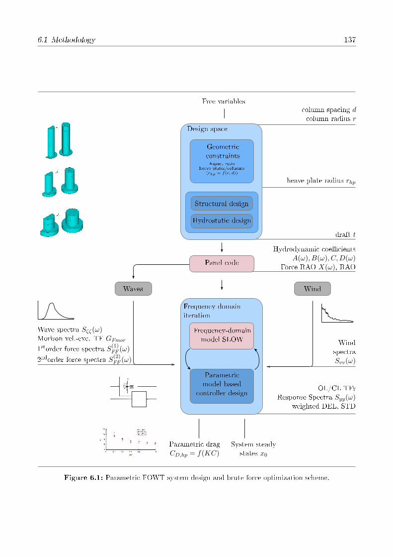
6.1 Methodology 137
Aspect ratioheave plates/columns
(rhp = f(r, d))
Geometricconstraints
Design space
Free variables
Structural design
Hydrostatic design
draft t
Panel code
Frequency-domainmodel SLOW
Waves
Wave spectra Sζζ(ω)Morison vel.-exc. TF GFmor
1storder force spectra S(1)FF (ω)
2ndorder force spectra S(2)FF (ω)
Parametricmodel-based
controller design
Frequency-domainiteration
Hydrodynamic coecientsA(ω), B(ω), C,D(ω)
Force RAO X(ω), RAO
Wind
System steadystates x0
Parametric dragCD,hp = f(KC)
WindspectraSvv(ω)
OL/CL TFsResponse Spectra Syy(ω)
weighted DEL, STD
column spacing dcolumn radius r
heave plate radius rhp
Figure 6.1: Parametric FOWT system design and brute-force optimization scheme.
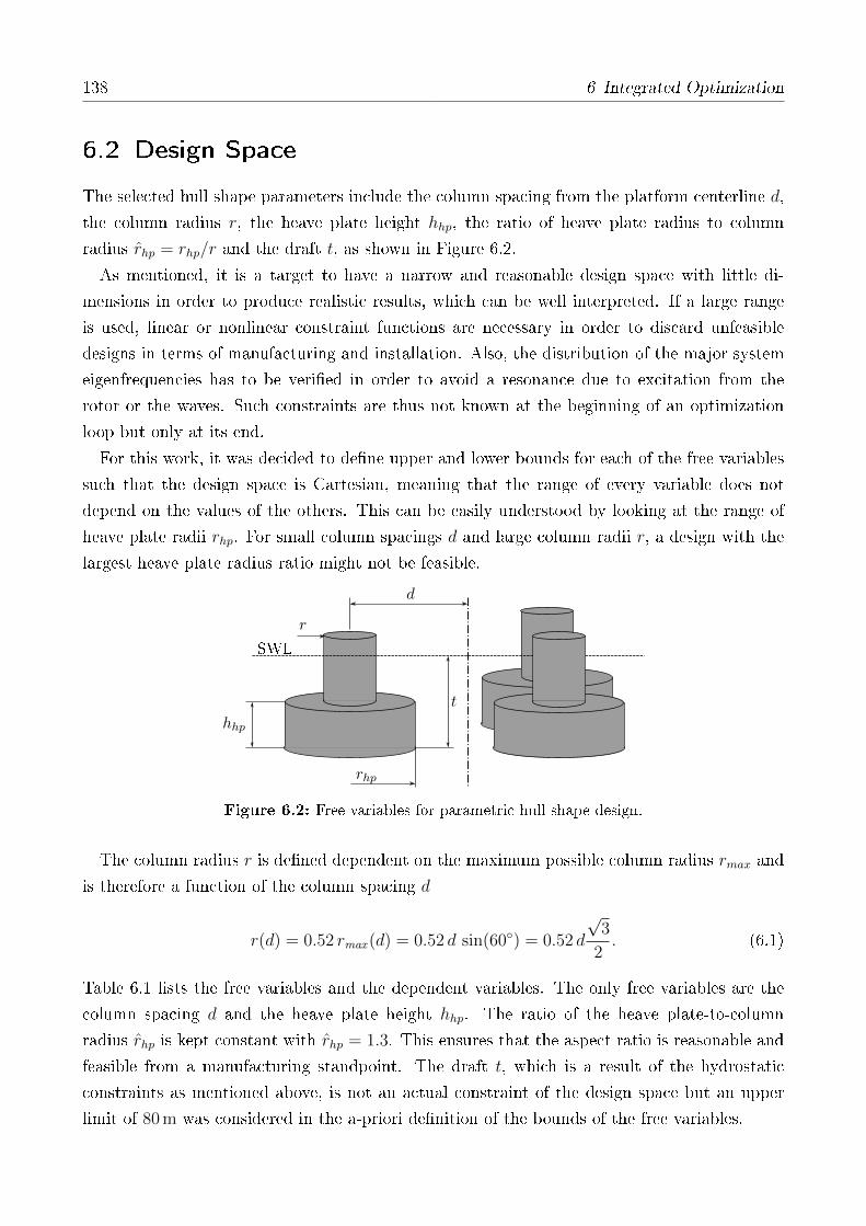
138 6 Integrated Optimization
6.2 Design Space
The selected hull shape parameters include the column spacing from the platform centerline d,
the column radius r, the heave plate height hhp, the ratio of heave plate radius to column
radius rhp = rhp/r and the draft t, as shown in Figure 6.2.
As mentioned, it is a target to have a narrow and reasonable design space with little di-
mensions in order to produce realistic results, which can be well interpreted. If a large range
is used, linear or nonlinear constraint functions are necessary in order to discard unfeasible
designs in terms of manufacturing and installation. Also, the distribution of the major system
eigenfrequencies has to be veried in order to avoid a resonance due to excitation from the
rotor or the waves. Such constraints are thus not known at the beginning of an optimization
loop but only at its end.
For this work, it was decided to dene upper and lower bounds for each of the free variables
such that the design space is Cartesian, meaning that the range of every variable does not
depend on the values of the others. This can be easily understood by looking at the range of
heave plate radii rhp. For small column spacings d and large column radii r, a design with the
largest heave plate radius ratio might not be feasible.
d
r
hhp
rhp
SWL
t
Figure 6.2: Free variables for parametric hull shape design.
The column radius r is dened dependent on the maximum possible column radius rmax and
is therefore a function of the column spacing d
r(d) = 0.52 rmax (d) = 0.52 d sin(60) = 0.52 d
√3
2. (6.1)
Table 6.1 lists the free variables and the dependent variables. The only free variables are the
column spacing d and the heave plate height hhp. The ratio of the heave plate-to-column
radius rhp is kept constant with rhp = 1.3. This ensures that the aspect ratio is reasonable and
feasible from a manufacturing standpoint. The draft t, which is a result of the hydrostatic
constraints as mentioned above, is not an actual constraint of the design space but an upper
limit of 80 m was considered in the a-priori denition of the bounds of the free variables.
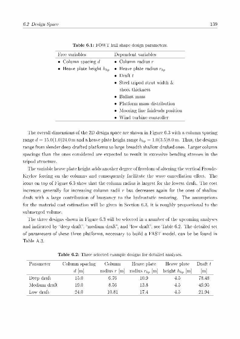
6.2 Design Space 139
Table 6.1: FOWT hull shape design parameters.
Free variables Dependent variables
• Column spacing d • Column radius r• Heave plate height hhp • Heave plate radius rhp
• Draft t• Steel tripod strut width &sheet thickness
• Ballast mass• Platform mass distribution• Mooring line fairleads position• Wind turbine controller
The overall dimensions of the 2D design space are shown in Figure 6.3 with a column spacing
range d = 15.0(1.0)24.0 m and a heave plate height range hhp = 1.0(3.5)8.0 m. Thus, the designs
range from slender deep-drafted platforms to large-breadth shallow-drafted ones. Larger column
spacings than the ones considered are expected to result in excessive bending stresses in the
tripod structure.
The variable heave plate height adds another degree of freedom of altering the vertical Froude-
Krylov forcing on the columns and consequently facilitate the wave cancellation eect. The
icons on top of Figure 6.3 show that the column radius is largest for the lowest draft. The cost
increases generally for increasing column radii r but decreases again for the ones of shallow
draft with a large contribution of buoyancy to the hydrostatic restoring. The assumptions
for the material cost estimation will be given in Section 6.3, it is roughly proportional to the
submerged volume.
The three designs shown in Figure 6.3 will be selected in a number of the upcoming analyses
and indicated by deep draft, medium draft, and low draft, see Table 6.2. The detailed set
of parameters of these three platforms, necessary to build a FAST model, can be be found in
Table A.3.
Table 6.2: Three selected example designs for detailed analyses.
Parameter Column spacing Column Heave plate Heave plate Draft td [m] radius r [m] radius rhp [m] height hhp [m] [m]
Deep draft 15.0 6.76 10.9 4.5 78.48Medium draft 19.0 8.56 13.8 4.5 49.95Low draft 24.0 10.81 17.4 4.5 21.94
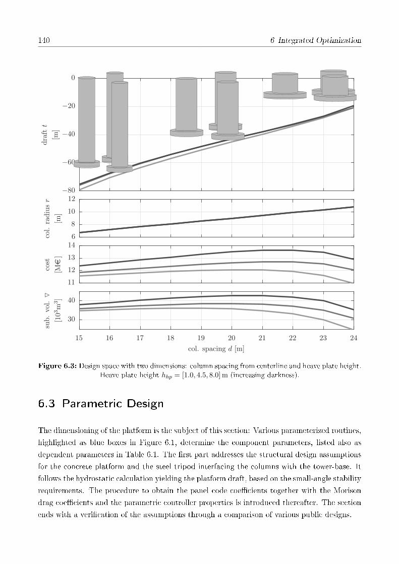
140 6 Integrated Optimization
col. spacing d [m]
sub.
vol.
[103
m3]
cost
[Me]
col.
radiu
sr
[m]
dra
ftt
[m]
15 16 17 18 19 20 21 22 23 24
30
40
11
12
13
146
8
10
12−80
−60
−40
−20
0
Figure 6.3: Design space with two dimensions: column spacing from centerline and heave plate height.Heave plate height hhp = [1.0, 4.5, 8.0] m (increasing darkness).
6.3 Parametric Design
The dimensioning of the platform is the subject of this section: Various parameterized routines,
highlighted as blue boxes in Figure 6.1, determine the component parameters, listed also as
dependent parameters in Table 6.1. The rst part addresses the structural design assumptions
for the concrete platform and the steel tripod interfacing the columns with the tower-base. It
follows the hydrostatic calculation yielding the platform draft, based on the small-angle stability
requirements. The procedure to obtain the panel code coecients together with the Morison
drag coecients and the parametric controller properties is introduced thereafter. The section
ends with a verication of the assumptions through a comparison of various public designs.

6.3 Parametric Design 141
6.3.1 Structural design
Approximate but realistic assumptions for the structural design make it possible to obtain the
mass distribution for the overall system simulations. The entire oater is assumed to be rigid
but the dimensions are selected reasonably to ensure structural integrity. Further design steps
are expected to detail the structural design without substantially changing the values obtained
from the presented approximations. The material properties for the following calculations are
listed in Table 6.3.
Table 6.3: Structural design assumptions.
Parameter Unit Value
Concrete column wall thickness [m] 0.6Heave plate upper and lower lid thickness [m] 0.4Reinforced concrete average density [kg/m3] 2750.0Steel density [kg/m3] 7750.0Ballast density [kg/m3] 2500.0Processed steel cost [e/t] 4500Processed concrete cost [e/t] 399
Steel tripod
The steel tripod design is based on an approximation from public data of the Bard Tripile, sup-
porting a 5 MW wind turbine. For a parameterization of the dimensions of the steel legs (shell
thickness, width, height), FE analyses were performed covering the design space of the distance
between the columns. The calculations include a static thrust load at the tower-top of 4.605 kN,
as given in [42, p. 61].
The critical failure mode is assumed to be the notch stress at the interface between the tower
and the legs. The dimensions of the legs (struts) are selected such that the maximum notch
stress at the interface of the legs with the tower is of comparable magnitude as the one resulting
from the same calculation with the Bard tripile. The dimensions of the tripod for the minimum
and the maximum column spacing are shown in Table 6.4. The Bard tripile data is no longer
available online but the details on the upscaling can be found in [233]. The structural design
of the TripleSpar concept, which started in 2015, was continued in the project INNWIND.EU
with the detailed design calculations of the substructure presented in [233] and [254].
Concrete columns and heave plates
The concrete columns are assumed to be built with pre-stressed concrete following the example
of the KIC-AFOSP spar design [202]. The wall thickness is constant for all of the hull shape

142 6 Integrated Optimization
Table 6.4: Parametric design of the TripleSpar steel tripod (FE calculations by Florian Amann).
Minimum column spacing Maximum column spacing
50 mm
5 m
60 mm
7 m
Column spacing10.0 m 35.0 m
(distance to centerline)Strut width & height 5.0 m 7.0 m
Steel wall thickness 50 mm 60 mm
Maximum stress 146.0 N/mm2 142.0 N/mm2
Tripod mass 447 t 1716 t
variations, see Table 6.3. The heave plates are also made out of reinforced concrete with the
same material properties as the columns. The columns reach down to the keel with heave
plates consisting of concrete rings attached to the columns at their lower end. This assumption
is rather conservative and accounts for further compartmentation and reinforcements of the
detailed design phase. The design of the baseline TripleSpar concept of Section 2.10 has heave
plates out of sheet metal and is therefore not directly comparable. The column wall thickness
of the TripleSpar is 0.4 m.
Mooring lines
The mooring line characteristics can be found in [58]. They were designed by myself to-
gether with Michael Borg of DTU with two upwind lines and one downwind line with fairleads
above SWL, at zfrlds = 8.7 m and a distance from the tower centerline of dfrlds = 26 m. The
same mooring system was used for the scaled experiments of Chapter 4. The parameters of the
mooring lines can be found in Appendix A.

6.3 Parametric Design 143
Tower
The tower design is not varied in the optimization study but the parameters of the refer-
ence TripleSpar are used, see Table A.1. Regarding the placement of resonances with respect
to the rotational frequencies, the present method assumes a rather small design space, which
is dened based on experience and preceding spreadsheet calculations. Therefore, the scatter
of platform eigenfrequencies is limited and consequently no adaptation of the tower stiness
to the substructure stiness is necessary. As mentioned in Section 3.8, the tower design can
generally be a bottleneck for wind turbines as large as 10 MW, due to tower excitation from
the 3p-frequency. The shown results for the present designs in Figures 6.196.23 indicate that
the response of the tower at the eigenfrequency of fd,twr = 0.416 Hz is at the analyzed wind
speeds, below and above rated, rather small compared to the response to waves. Therefore, the
tower design is expected not to alter the ndings of the present platform optimization study.
Cost estimation
In dierent research projects cost models for FOWTs were presented with a good overview and
summary in [255]. In the present work, a lumped cost for the processed material, meaning the
sum of the material, manufacturing and assembly costs, is assumed. The values are according
to LIFES50+ Deliverable 4.3 [251] and can be found in Table 6.3. It needs to be mentioned
that these values are rough indications, which can vary due to concrete shrinkage (concrete
prices are, as opposed to steel, usually not given per mass but per volume) and also due to
price variations over time.
6.3.2 Hydrostatic design
The hydrostatic properties determine mainly the FOWT stability and the system eigenfrequen-
cies together with the mass distribution, see also Section 2.5.3. If no active ballast system is
included, the hydrostatic restoring in pitch-direction determines, together with the vertical dis-
tance between the fairleads and the hub, the inclination of the rotor to the vertical plane and
therefore the power losses, which deteriorate the eciency by ηcos ∝ cos3(βrotor). The nonlinear
intact stability criteria are relevant for certication and might challenge designs with a soft
pitch stiness C55. Another constraint for the maximum (dynamic) pitch angle is the wind
turbine gearbox and other components requiring an upright operational position.
For the present study, a hydrostatic restoring in pitch of C55 = 2.255× 10⁹ Nm/rad, resulting
in a steady state platform pitch angle at rated wind speed (disregarding again the mooring
line restoring) of βp,rated = 5.0 deg, is set as constraint for all geometries of the design space.
Depending on the free variables column spacing d and heave plate height hhp, the draft is
determined such that this constraint is met. This is realized through a root-nding algorithm

144 6 Integrated Optimization
including the structural design and the hydrostatic functions. The steady state pitch angle
reduces to about βp,rated ≈ 3.0 deg with the mooring lines.
6.3.3 Hydrodynamic coecients
The parametric calculation of the hydrodynamic coecients is performed with Ansys Aqwa
with a generation of the parameterized hull geometries by Ansys APDL. The added mass
is then interpolated at the respective eigenfrequencies and transformed to the platform CM,
according to Section 3.5.3. The radiation damping B(ω) is neglected in the analysis of this
chapter based on the discussion of Section 3.5.1 and the ndings of the sensitivity study of
Section 6.4.6. The mean drift force coecient D(ω) is calculated for all designs and used for
Newman's approximation on the dierence-frequency excitation, see Figure 6.1.
The column drag coecient is kept constant for all designs and sea-states. It has been selected
as CD = 0.4 because this value was also identied in the scaled experiments of Chapter 4. The
selected value is rather conservative, as guidelines suggest minimum values of CD = 0.65,
see [256, p. 117]. For the heave plates, the drag coecient is iterated based on the drag
coecients given in [230], which were parameterized as a function of KC , see Section 4.4. In
order to reduce the problem complexity, the vertical drag force is applied only at the lower
surface of the heave plates and the same cross-sectional area is used for the calculation of the
drag force. The procedure was introduced in Section 3.5, see Figure 3.18.
With the increase of the heave plate radius r, the characteristics of the hydrodynamic forces
change. The wave regime graph, Figure 2.4, shows the values of the Keulegan-Carpenter
number KC and the diraction parameter ka for the deep-draft (slender columns) and the low-
draft (big columns) design. It can be seen that diraction becomes more important for smaller
sea-states and the drag component of the forcing increases with decreasing column diameters.
The vertical drag due to heave plates, on the other side, is not covered by Figure 2.4. This
vertical drag becomes more important for increasing heave plate diameters, see Section 3.5.
This is a nonlinear eect (quadratic drag), which yields simulation errors when the linearized
model is used, see Section 6.4.5.
6.3.4 Controller design
For each of the concepts of the design space (Figure 6.3), a SISO PI-controller and a MIMO LQ-
controller is designed. The controllers have the architecture of the ones described in Chapter 5.
The advantage of the MIMO controller is that it feeds back more signals and uses the generator
torque as additional actuator to the blade pitch angle. It has therefore a higher potential
to improve rotor speed tracking and disturbance rejection. As all states of the simulation
model are fed back, disregarding the question of how to measure or observe them in reality,
6.3 Parametric Design 145
this controller is seen as a means to obtain an upper bound of the possible performance of
an optimal controller. The straightforward model-based design makes this controller perfectly
suited for this integrated design study.
However, it was found that the advantages of specic gains on e.g. platform pitch βp depend
signicantly on the platform shape. Therefore, the comparison of the simple SISO controller
oers a means to evaluate the fairness of the LQR towards dierent platform shapes. The SISO
controller ensures the same stability for all shapes and does not feed back any states other than
the two rotor rotation states. A special challenge with the LQR design is the fact that damping
the wave response by feeding back system states is not possible and might even increase the
response, see [183] and discussions in Chapter 5. This can result in a reasonable response to
wave for one design but in a amplication for another design. The main reason for this is that
the system response depends signicantly on the characteristics of the force-RAO X(ω), which
is not part of the system matrix A but the input matrix B and therefore not taken into account
by the LQR design routine. For this reason, the determination of the matrices Q, R and N
was made considering all platforms of the design space resulting in the values of Table 5.2.
The new parameterization of the SISO PI-controller was introduced in Section 5.3. The
criterion of the maximum sensitivity 1/Ms and the rotor time constant τrot, introduced in
Chapter 5, allow for an automation. As opposed to the MIMO controller, the PI-controllers
are designed based on the models, linearized at all operational wind speeds above rated. This
yields the gain scheduling function of Figure 6.4, including the switching criterion between the
stability objective for wind speeds above rated and the one of a constant τrot, see Section 5.3.
The LQR can be designed for each operating point independently and makes the iterative
determination of the viscous drag, introduced in Section 3.5.4, easier.
Figure 6.4 shows the feedback gains for the three example designs of the design space for
the LQR and PI-controllers over above-rated wind speeds. Generally, the gains of the deep-
drafted platform dier from the medium- and low-draft platform. A reason might be the
dierent platform pitch-mode frequency and damping as will be shown in Figure 6.7. The two
upper rows show the feedback gains of the generator speed, not as state feedback gains of ϕ
and Ω but as proportional gain kp and integrator time constant Ti of an equivalent PI-controller,
see Figure 5.5. It can be seen that the proportional gains kp of the LQR are signicantly larger
than those of the PI-controller. This means that the additional damping of the platform
and tower, through the tower and platform velocity feedback, allows for a more aggressively
tuned rotor speed control loop. The same approach was selected by [183], who maintained the
onshore gains for the FOWT and added additional feedback loops for platform stabilization.
The question of stability, however, is then not resolved, as is also the case for the LQR, which
might have limited stability margins. The integrator time constant Ti does not change over the
wind speeds for the PI-controller, see Section 5, but decreases for the LQR.
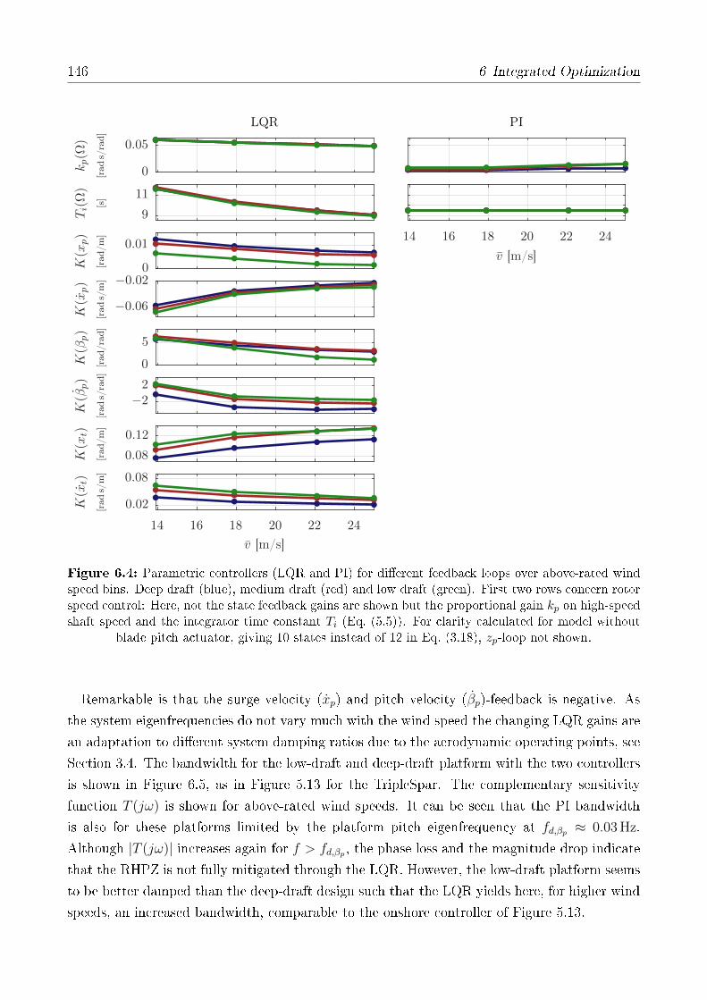
146 6 Integrated Optimization
LQR PI
v [m/s]
K(x
t)
[rad
s/m]
K(x
t)
[rad/m]
K(β
p)
[rad
s/ra
d]
K(β
p)
[rad/ra
d]
K(x
p)
[rad
s/m]
K(x
p)
[rad/m]
Ti(Ω)
[s]
kp(Ω
)
[rad
s/ra
d]
v [m/s]
14 16 18 20 22 24
14 16 18 20 22 24
0.02
0.08
0.08
0.12
−22
0
5
−0.06
−0.020
0.01
9
11
0
0.05
Figure 6.4: Parametric controllers (LQR and PI) for dierent feedback loops over above-rated windspeed bins. Deep draft (blue), medium draft (red) and low draft (green). First two rows concern rotorspeed control: Here, not the state feedback gains are shown but the proportional gain kp on high-speedshaft speed and the integrator time constant Ti (Eq. (5.5)). For clarity calculated for model without
blade pitch actuator, giving 10 states instead of 12 in Eq. (3.18), zp-loop not shown.
Remarkable is that the surge velocity (xp) and pitch velocity (βp)-feedback is negative. As
the system eigenfrequencies do not vary much with the wind speed the changing LQR gains are
an adaptation to dierent system damping ratios due to the aerodynamic operating points, see
Section 3.4. The bandwidth for the low-draft and deep-draft platform with the two controllers
is shown in Figure 6.5, as in Figure 5.13 for the TripleSpar. The complementary sensitivity
function T (jω) is shown for above-rated wind speeds. It can be seen that the PI bandwidth
is also for these platforms limited by the platform pitch eigenfrequency at fd,βp ≈ 0.03 Hz.
Although |T (jω)| increases again for f > fd,βp , the phase loss and the magnitude drop indicate
that the RHPZ is not fully mitigated through the LQR. However, the low-draft platform seems
to be better damped than the deep-draft design such that the LQR yields here, for higher wind
speeds, an increased bandwidth, comparable to the onshore controller of Figure 5.13.

6.3 Parametric Design 147
d = 24m, r = 10.8md = 15m, r = 6.8m
frequency [Hz]frequency [Hz]
LQ
R
∠T(jω)[−
]
LQ
R
|T(jω)|[−
]
PI
∠T(jω)[−
]
PI
|T(jω)|[−
]
0 0.1 0.2 0.30 0.1 0.2 0.3
−360
00
0.5
1
−360
00
0.5
1
Figure 6.5: Complementary sensitivity T (jω) magnitude and phase for PI-controller (top)and LQR (bottom) for deep draft (left) and low draft (right) designs over above-rated wind speeds.Lighter line color for higher wind speeds v0 = [13.9, 17.9, 22.1, 25] m/s. First intersection of T (jω)
with dashed line indicates bandwidth.
6.3.5 Design verication
Especially for the concrete columns and heave plates, no structural design calculations have
been performed but the numbers are based on the project KIC-AFOSP on which I worked
in the course of this thesis. Therefore, the structural design assumptions are veried through
a comparison with other public FOWT designs. The platform mass distribution is taken as
indicator, represented by the platform center of mass zcm,ptfm and the overall FOWT center of
mass zcm,fowt , including the wind turbine (without mooring lines).
For semi-submersibles and spars, an eective design has a mass concentration at the lowest
possible point, close to the keel, in order to maximize the restoring moment from the gravita-
tional forces. Then the center-of-mass-ratio zcm/t approaches a value of 1. Such high values
of zcm/t are not possible in reality, due to the plating, stieners and girders, compartmentation
and secondary steel, the elements resulting from the detailed structural design, which is not
included in the present dimensioning. These elements sum up to a signicant amount of mass
at higher levels, elevating the center of mass and decreasing the hydrostatic stability.
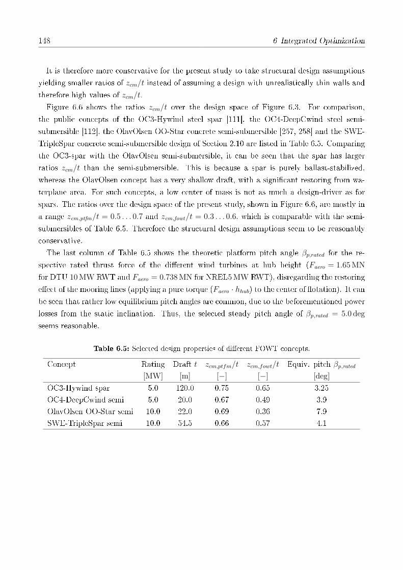
148 6 Integrated Optimization
It is therefore more conservative for the present study to take structural design assumptions
yielding smaller ratios of zcm/t instead of assuming a design with unrealistically thin walls and
therefore high values of zcm/t.
Figure 6.6 shows the ratios zcm/t over the design space of Figure 6.3. For comparison,
the public concepts of the OC3-Hywind steel spar [111], the OC4-DeepCwind steel semi-
submersible [112], the OlavOlsen OO-Star concrete semi-submersible [257, 258] and the SWE-
TripleSpar concrete semi-submersible design of Section 2.10 are listed in Table 6.5. Comparing
the OC3-spar with the OlavOlsen semi-submersible, it can be seen that the spar has larger
ratios zcm/t than the semi-submersible. This is because a spar is purely ballast-stabilized,
whereas the OlavOlsen concept has a very shallow draft, with a signicant restoring from wa-
terplane area. For such concepts, a low center of mass is not as much a design-driver as for
spars. The ratios over the design space of the present study, shown in Figure 6.6, are mostly in
a range zcm,ptfm/t = 0.5 . . . 0.7 and zcm,fowt/t = 0.3 . . . 0.6, which is comparable with the semi-
submersibles of Table 6.5. Therefore the structural design assumptions seem to be reasonably
conservative.
The last column of Table 6.5 shows the theoretic platform pitch angle βp,rated for the re-
spective rated thrust force of the dierent wind turbines at hub height (Faero = 1.65 MN
for DTU 10 MW RWT and Faero = 0.738 MN for NREL5 MW RWT), disregarding the restoring
eect of the mooring lines (applying a pure torque (Faero · hhub) to the center of otation). It canbe seen that rather low equilibrium pitch angles are common, due to the beforementioned power
losses from the static inclination. Thus, the selected steady pitch angle of βp,rated = 5.0 deg
seems reasonable.
Table 6.5: Selected design properties of dierent FOWT concepts.
Concept Rating Draft t zcm,ptfm/t zcm,fowt/t Equiv. pitch βp,rated[MW] [m] [−] [−] [deg]
OC3-Hywind spar 5.0 120.0 0.75 0.65 3.25OC4-DeepCwind semi 5.0 20.0 0.67 0.49 3.9OlavOlsen OO-Star semi 10.0 22.0 0.69 0.36 7.9SWE-TripleSpar semi 10.0 54.5 0.66 0.57 4.1

6.4 Results 149
column spacing d [m]
z cm,fowt/t
[-]
z cm,ptfm/t
[-]
15 16 17 18 19 20 21 22 23 24
0.2
0.4
0.6
0.5
0.6
0.7
Figure 6.6: Ratio of platform center of mass-to-draft and ratio of overall FOWT center of mass-to-draft over design space. Heave plate height hhp = [1.0, 4.5, 8.0] m (increasing darkness).
6.4 Results
In this section, the results of full operational DLCs over the design space are shown together
with linear system analyses revealing the physical reasons for advantages or disadvantages of
dierent platform geometries reected in the DLC results. Subsequently, the entire design space
is simulated with the simplied models (linear and nonlinear) and the full FAST model and
dierent modeling options for comparisons and an assessment of the model delity over the
design space.
6.4.1 Linear system analysis of open loop system
Figure 6.7 shows the results of the eigenanalysis over the design space using the simplied lin-
earized model in the open loop conguration. Compared to a simpler eigenanalysis with a panel
code (assuming a single rigid body, linearized mooring stinesses and 1st-order hydrodynamics),
the following features are included in SLOW:
• linearized aerodynamics of entire rotor, rotor-DoF
• exible tower (1st mode)
• mooring stiness linearized about operating point
• linearized Morison drag
Therefore, the eigenmodes of the platform can be expected to be more accurate than the
ones predicted by the panel code, especially due to the inclusion of the hydrodynamic viscous
drag, the tower and aerodynamics. The controller dynamics are not included here but they
are subject of the next section. The two columns of Figure 6.7 contain the minimum and
maximum heave plate thickness hhp = [1.0, 8.0] m while the column spacing d is on the x-axis
of each graph. The two top rows show the surge and pitch eigenfrequencies and the lower rows
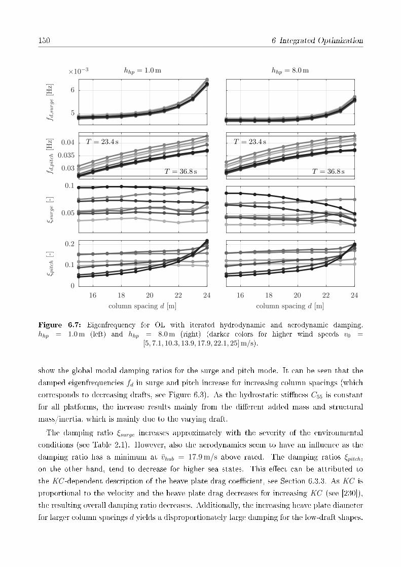
150 6 Integrated Optimization
T = 36.8 s
T = 23.4 s
hhp = 8.0m
T = 36.8 s
T = 23.4 s
hhp = 1.0m
column spacing d [m]column spacing d [m]
ξ pitch
[-]
ξ surge[-]
f d,pitch
[Hz]
f d,surge[H
z]
16 18 20 22 2416 18 20 22 24
×10−3
0
0.1
0.2
0.05
0.1
0.03
0.035
0.04
5
6
Figure 6.7: Eigenfrequency for OL with iterated hydrodynamic and aerodynamic damping.hhp = 1.0 m (left) and hhp = 8.0 m (right) (darker colors for higher wind speeds v0 =
[5, 7.1, 10.3, 13.9, 17.9, 22.1, 25] m/s).
show the global modal damping ratios for the surge and pitch mode. It can be seen that the
damped eigenfrequencies fd in surge and pitch increase for increasing column spacings (which
corresponds to decreasing drafts, see Figure 6.3). As the hydrostatic stiness C55 is constant
for all platforms, the increase results mainly from the dierent added mass and structural
mass/inertia, which is mainly due to the varying draft.
The damping ratio ξsurge increases approximately with the severity of the environmental
conditions (see Table 2.1). However, also the aerodynamics seem to have an inuence as the
damping ratio has a minimum at vhub = 17.9 m/s above rated. The damping ratios ξpitch,
on the other hand, tend to decrease for higher sea states. This eect can be attributed to
the KC -dependent description of the heave plate drag coecient, see Section 6.3.3. As KC is
proportional to the velocity and the heave plate drag decreases for increasing KC (see [230]),
the resulting overall damping ratio decreases. Additionally, the increasing heave plate diameter
for larger column spacings d yields a disproportionately large damping for the low-draft shapes.

6.4 Results 151
6.4.2 Linear system analysis of closed loop system
The eigenanalysis in the closed-loop for the two controllers of Chapter 5 is shown in Figure 6.8.
Comparing the values to the open loop case of Figure 6.7, it can be seen that the damped surge
eigenfrequencies are comparable but tend to higher frequencies due to the introduced controller
dynamics.
T = 40.9 s
T = 23.7 s
LQR
T = 40.9 s
T = 23.7 s
PI
column spacing d [m]column spacing d [m]
f 0,rot[H
z]ξ p
itch
[-]
ξ surge[-]
f d,pitch
[Hz]
f d,surge[H
z]
16 18 20 22 2416 18 20 22 24
×10−3
0.01
0.02
0
0.1
0.2
0.05
0.1
0.025
0.035
4
5
6
7
Figure 6.8: Eigenfrequency for CL with iterated hydrodynamic and aerodynamic damping.PI-controller (left) and LQR-controller (right) (darker colors for higher wind speeds v0 =
[5, 7.1, 10.3, 13.9, 17.9, 22.1, 25] m/s).
In pitch-direction, it can be observed that the platform eigenfrequency increases for above-
rated wind speeds vhub = [13.9, 17.9, 22.1, 25] m/s. The same eect was visible for the exper-
iments, Chapter 4, and can be seen even more clearly in Figure 6.13. The damping ratio ξ
also changes with closing the control loop: While in surge-direction the controller aects most
the below-rated damping ratios, there is a clear change of damping in pitch-direction for the
above-rated wind speeds (darker colors). There is less damping in pitch for the PI-controller,
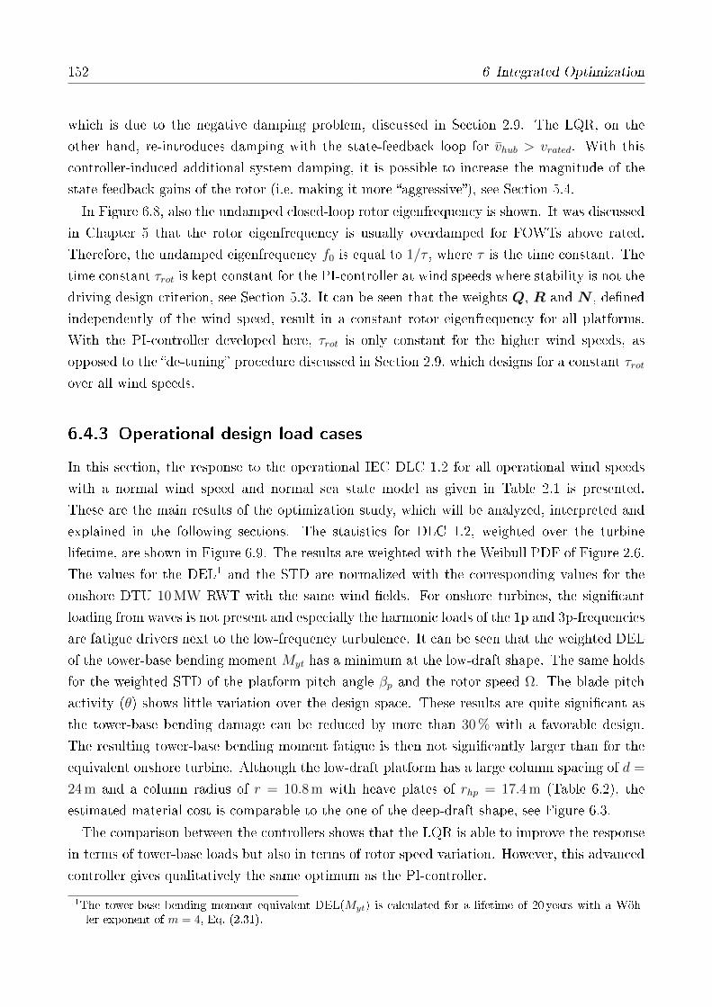
152 6 Integrated Optimization
which is due to the negative damping problem, discussed in Section 2.9. The LQR, on the
other hand, re-introduces damping with the state-feedback loop for vhub > vrated. With this
controller-induced additional system damping, it is possible to increase the magnitude of the
state feedback gains of the rotor (i.e. making it more aggressive), see Section 5.4.
In Figure 6.8, also the undamped closed-loop rotor eigenfrequency is shown. It was discussed
in Chapter 5 that the rotor eigenfrequency is usually overdamped for FOWTs above rated.
Therefore, the undamped eigenfrequency f0 is equal to 1/τ , where τ is the time constant. The
time constant τrot is kept constant for the PI-controller at wind speeds where stability is not the
driving design criterion, see Section 5.3. It can be seen that the weights Q, R and N , dened
independently of the wind speed, result in a constant rotor eigenfrequency for all platforms.
With the PI-controller developed here, τrot is only constant for the higher wind speeds, as
opposed to the de-tuning procedure discussed in Section 2.9, which designs for a constant τrotover all wind speeds.
6.4.3 Operational design load cases
In this section, the response to the operational IEC DLC 1.2 for all operational wind speeds
with a normal wind speed and normal sea state model as given in Table 2.1 is presented.
These are the main results of the optimization study, which will be analyzed, interpreted and
explained in the following sections. The statistics for DLC 1.2, weighted over the turbine
lifetime, are shown in Figure 6.9. The results are weighted with the Weibull PDF of Figure 2.6.
The values for the DEL1 and the STD are normalized with the corresponding values for the
onshore DTU 10 MW RWT with the same wind elds. For onshore turbines, the signicant
loading from waves is not present and especially the harmonic loads of the 1p and 3p-frequencies
are fatigue drivers next to the low-frequency turbulence. It can be seen that the weighted DEL
of the tower-base bending momentMyt has a minimum at the low-draft shape. The same holds
for the weighted STD of the platform pitch angle βp and the rotor speed Ω. The blade pitch
activity (θ) shows little variation over the design space. These results are quite signicant as
the tower-base bending damage can be reduced by more than 30 % with a favorable design.
The resulting tower-base bending moment fatigue is then not signicantly larger than for the
equivalent onshore turbine. Although the low-draft platform has a large column spacing of d =
24 m and a column radius of r = 10.8 m with heave plates of rhp = 17.4 m (Table 6.2), the
estimated material cost is comparable to the one of the deep-draft shape, see Figure 6.3.
The comparison between the controllers shows that the LQR is able to improve the response
in terms of tower-base loads but also in terms of rotor speed variation. However, this advanced
controller gives qualitatively the same optimum as the PI-controller.
1The tower-base bending moment equivalent DEL(Myt) is calculated for a lifetime of 20 years with a Wöh-ler exponent of m = 4, Eq. (2.31).

6.4 Results 153
PSfrag replacements
LQRPI
column spacing d [m]column spacing d [m]
ST
D(θ
)[-]
ST
D(Ω
)[-]
ST
D(β
p)[d
eg]
DE
L(M
yT)[-]
16 18 20 22 2416 18 20 22 24
0.4
0.5
0.5
1
0.4
0.6
0.81
1.5
2
2.5
Figure 6.9: Response statistics of operational DLC1.2, Tab 2.1, weighted for all wind speeds withdistribution of Figure 2.6. DEL/STD are normalized results with corresponding SLOW onshore sim-ulations of DTU 10 MW RWT with the same wind elds. Left PI-controller, right LQR-controller.
Heave plate height hhp = [1.0, 4.5, 8.0] m (increasing darkness).
One nding from this is that the low-frequency platform pitch response to wind and dierence-
frequency excitations is likely not the reason for the improved performance of the low-draft
shape as these resonances are damped by the LQR.
A comparison of the response spectra among the deep draft and the low draft platforms with
the PI-controller is shown in Figure 6.10. Since the magnitudes are signicantly dierent, a
logarithmic y-axis is selected. It can be seen that the low-draft shape gives a larger dierence-
frequency and wind-induced response in surge. Other than this, the low-draft platform has
clearly smaller responses at the pitch eigenfrequency of fd ,pitch ≈ 0.04 Hz but, more impor-
tantly, at the wave frequencies of 0.1 Hz (vhub = 17.9 m/s, left) and 0.08 Hz (vhub = 25 m/s,
right). This is visible for the platform motion response βp but even more for the tower
bending (xt, Myt), the rotor speed Ω and the electrical power P .
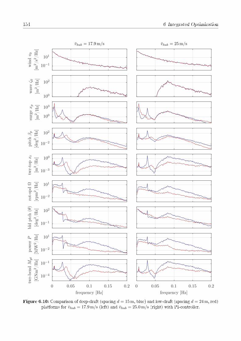
154 6 Integrated Optimization
PSfrag replacements
vhub = 25m/svhub = 17.9m/s
frequency [Hz]frequency [Hz]
twr-
ben
dM
yt
[GN
m2/H
z]
pow
erP
[MW
2/H
z]
bld
ptc
h(θ
)
[deg
2/H
z]
rot-
spdΩ
[rpm
2/H
z]
twr-
topxt
[m2/H
z]
pit
chβp
[deg
2/H
z]
surg
exp
[m2/H
z]
wav
eζ 0
[m2/H
z]
win
dv 0
[m2/s
2/H
z]
0 0.05 0.1 0.15 0.20 0.05 0.1 0.15 0.2
10−4
10−1
10−2
101
10−1
102
10−2
101
10−3
100
10−2
102
100
103
100
102
10−1
101
Figure 6.10: Comparison of deep-draft (spacing d = 15 m, blue) and low-draft (spacing d = 24 m, red)platforms for vhub = 17.9 m/s (left) and vhub = 25.0 m/s (right) with PI-controller.

6.4 Results 155
The validity of the controllers is shown in Figure 6.11 in terms of the criteria dened in
Table 2.2. The maximum amplitude is here estimated from the frequency-domain response
spectra for a time of T = 3600 s with the Rayleigh distribution for the response amplitudes as
described in Section 2.7.3. It can be seen that keeping the limits for a FOWT is challenging.
This is mainly due to the reduced bandwidth of the controller. The overshoot of the rotor speed
can be signicantly reduced by feeding back additional signals and by using the generator torque
as an actuator above rated. Then, however, it is important to design the controller such that
the torque limits are not exceeded. Here, the LQR exceeds the rated torque up to 17 % for short
time periods. The power overshoot can be reduced by the LQR such that the limit of 15 % is
exceeded only for the highest waves.
LQRPI
column spacing d [m]column spacing d [m]
P[-]
Mg[-]
Ω[-]
16 18 20 22 2416 18 20 22 24
1
1.1
1.2
1
1.1
1.21
1.1
1.2
Figure 6.11: Rotor signals percentage of maximum over rated values (overshoot) for opera-tional DLC1.2, Tab 2.1 for above rated wind speeds v = [13.9 (4), 17.9 (+), 22.1 (), 25.0 (O)] m/s
for dierent column spacings d, hhp = 4.5 m. Left PI-controller, right LQR.
Comparing the PI-controller and the LQR, it can be seen that the largest amplitudes result
from wind speeds around rated, while it is the case for the cut-out wind speed for the LQR.
This is because the instability issue of FOWTs is critical at rated wind speeds as discussed in
Section 5.3, while the instability is mitigated through the LQR such that the high sea-states
drive the response amplitudes.
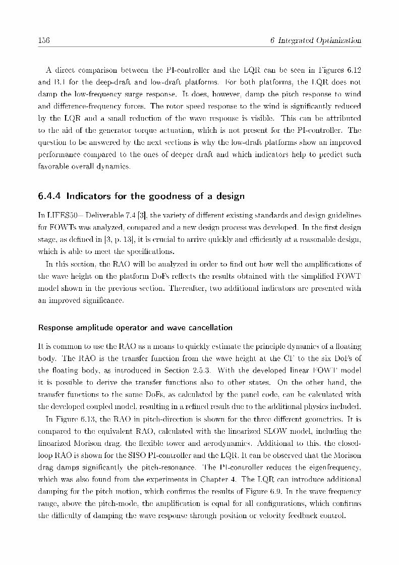
156 6 Integrated Optimization
A direct comparison between the PI-controller and the LQR can be seen in Figures 6.12
and B.1 for the deep-draft and low-draft platforms. For both platforms, the LQR does not
damp the low-frequency surge response. It does, however, damp the pitch response to wind
and dierence-frequency forces. The rotor speed response to the wind is signicantly reduced
by the LQR and a small reduction of the wave response is visible. This can be attributed
to the aid of the generator torque actuation, which is not present for the PI-controller. The
question to be answered by the next sections is why the low-draft platforms show an improved
performance compared to the ones of deeper draft and which indicators help to predict such
favorable overall dynamics.
6.4.4 Indicators for the goodness of a design
In LIFES50+ Deliverable 7.4 [3], the variety of dierent existing standards and design guidelines
for FOWTs was analyzed, compared and a new design process was developed. In the rst design
stage, as dened in [3, p. 13], it is crucial to arrive quickly and eciently at a reasonable design,
which is able to meet the specications.
In this section, the RAO will be analyzed in order to nd out how well the amplications of
the wave height on the platform DoFs reects the results obtained with the simplied FOWT
model shown in the previous section. Thereafter, two additional indicators are presented with
an improved signicance.
Response amplitude operator and wave cancellation
It is common to use the RAO as a means to quickly estimate the principle dynamics of a oating
body. The RAO is the transfer function from the wave height at the CF to the six DoFs of
the oating body, as introduced in Section 2.5.3. With the developed linear FOWT model
it is possible to derive the transfer functions also to other states. On the other hand, the
transfer functions to the same DoFs, as calculated by the panel code, can be calculated with
the developed coupled model, resulting in a rened result due to the additional physics included.
In Figure 6.13, the RAO in pitch-direction is shown for the three dierent geometries. It is
compared to the equivalent RAO, calculated with the linearized SLOW model, including the
linearized Morison drag, the exible tower and aerodynamics. Additional to this, the closed-
loop RAO is shown for the SISO PI-controller and the LQR. It can be observed that the Morison
drag damps signicantly the pitch-resonance. The PI-controller reduces the eigenfrequency,
which was also found from the experiments in Chapter 4. The LQR can introduce additional
damping for the pitch motion, which conrms the results of Figure 6.9. In the wave frequency
range, above the pitch-mode, the amplication is equal for all congurations, which conrms
the diculty of damping the wave response through position or velocity feedback control.
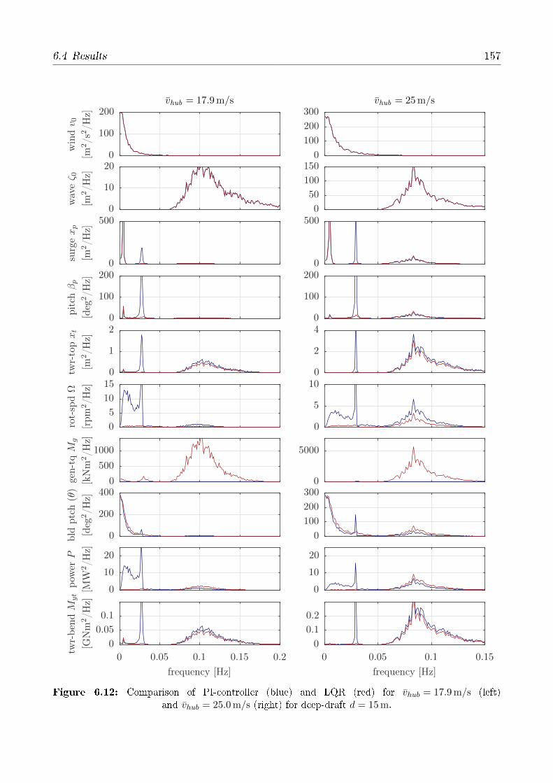
6.4 Results 157
PSfrag replacements
vhub = 25m/svhub = 17.9m/s
frequency [Hz]frequency [Hz]
twr-
ben
dM
yt
[GN
m2/H
z]
pow
erP
[MW
2/H
z]
bld
ptc
h(θ
)
[deg
2/H
z]
gen-t
qM
g
[kN
m2/H
z]
rot-
spdΩ
[rpm
2/H
z]
twr-
topxt
[m2/H
z]
pit
chβp
[deg
2/H
z]
surg
exp
[m2/H
z]
wav
eζ 0
[m2/H
z]
win
dv 0
[m2/s
2/H
z]
0 0.05 0.1 0.150 0.05 0.1 0.15 0.2
0
0.1
0.2
0
10
20
0
100
200
3000
5000
0
5
100
2
40
100
2000
5000
50
100
1500
100
200
300
0
0.05
0.1
0
10
20
0
200
4000
500
1000
0
5
10
150
1
20
100
2000
5000
10
200
100
200
Figure 6.12: Comparison of PI-controller (blue) and LQR (red) for vhub = 17.9 m/s (left)and vhub = 25.0 m/s (right) for deep-draft d = 15 m.
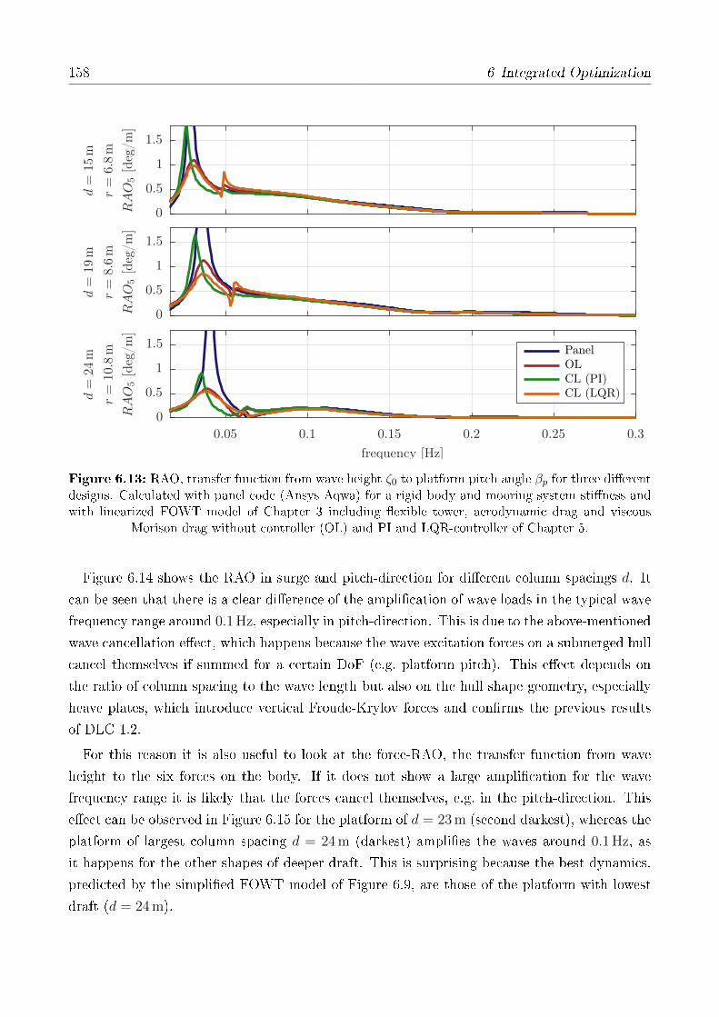
158 6 Integrated Optimization
PanelOLCL (PI)CL (LQR)
frequency [Hz]
d=
24m
r=
10.8
m
RAO
5[d
eg/m
]
d=
19m
r=
8.6
m
RAO
5[d
eg/m
]
d=
15m
r=
6.8
m
RAO
5[d
eg/m
]
0.05 0.1 0.15 0.2 0.25 0.3
0
0.5
1
1.5
0
0.5
1
1.5
0
0.5
1
1.5
Figure 6.13: RAO, transfer function from wave height ζ0 to platform pitch angle βp for three dierentdesigns. Calculated with panel code (Ansys Aqwa) for a rigid body and mooring system stiness andwith linearized FOWT model of Chapter 3 including exible tower, aerodynamic drag and viscous
Morison drag without controller (OL) and PI and LQR-controller of Chapter 5.
Figure 6.14 shows the RAO in surge and pitch-direction for dierent column spacings d. It
can be seen that there is a clear dierence of the amplication of wave loads in the typical wave
frequency range around 0.1 Hz, especially in pitch-direction. This is due to the above-mentioned
wave cancellation eect, which happens because the wave excitation forces on a submerged hull
cancel themselves if summed for a certain DoF (e.g. platform pitch). This eect depends on
the ratio of column spacing to the wave length but also on the hull shape geometry, especially
heave plates, which introduce vertical Froude-Krylov forces and conrms the previous results
of DLC 1.2.
For this reason it is also useful to look at the force-RAO, the transfer function from wave
height to the six forces on the body. If it does not show a large amplication for the wave
frequency range it is likely that the forces cancel themselves, e.g. in the pitch-direction. This
eect can be observed in Figure 6.15 for the platform of d = 23 m (second darkest), whereas the
platform of largest column spacing d = 24 m (darkest) amplies the waves around 0.1 Hz, as
it happens for the other shapes of deeper draft. This is surprising because the best dynamics,
predicted by the simplied FOWT model of Figure 6.9, are those of the platform with lowest
draft (d = 24 m).
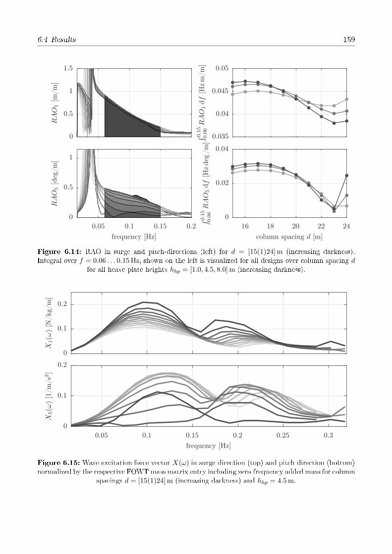
6.4 Results 159
PSfrag replacements
column spacing d [m]
∫ 0.15
0.06RAO
5df[H
zdeg
/m]
frequency [Hz]
RAO
5[d
eg/m
]
∫ 0.15
0.06RAO
1df[H
zm
/m]
RAO
1[m
/m]
16 18 20 22 240.05 0.1 0.15 0.2
0
0.02
0.04
0
0.5
1
0.035
0.04
0.045
0.05
0
0.5
1
1.5
Figure 6.14: RAO in surge and pitch-directions (left) for d = [15(1)24] m (increasing darkness).Integral over f = 0.06 . . . 0.15 Hz, shown on the left is visualized for all designs over column spacing d
for all heave plate heights hhp = [1.0, 4.5, 8.0] m (increasing darkness).
frequency [Hz]
X5(ω
)[1
/m/s
2]
X1(ω
)[N
/kg/
m]
0.05 0.1 0.15 0.2 0.25 0.3
0
0.1
0.2
0
0.1
0.2
Figure 6.15: Wave excitation force vector X(ω) in surge-direction (top) and pitch-direction (bottom)normalized by the respective FOWTmass matrix entry including zero-frequency added mass for column
spacings d = [15(1)24] m (increasing darkness) and hhp = 4.5 m.

160 6 Integrated Optimization
As an indicator of goodness of the design, the RAO is integrated over f = 0.06 . . . 0.15 Hz in
Figure 6.14. The results agree well with those of the simplied model, Figure 6.9, as the integral
decreases for larger spacings d. However, the RAO of Figure 6.14 increases again signicantly
for the largest spacing of d = 24 m in the same way as the force-RAO of Figure 6.15. The reason
why the largest spacing (d = 24 m) is underestimated by the RAO, as opposed to the DLC
results, is discussed in the next section.
Harmonic response
A key to understanding the underlying eect for the disturbance rejection of the low-draft
platform (d = 24 m) is the harmonic response to wind and wave loads. Figure 6.16 shows
lines representing the FOWT centerline. The horizontal displacement and orientation of each
line stands for the amplitude of the body response at all elevations along the centerline to
sinusoidal wind (top) and wave excitations (bottom) of dierent frequencies. The analysis is
made with the reduced order linearized model with rst-order hydrodynamics in closed-loop
with the PI-controller at vhub = 13.9 m/s. It is noted that the controller does not signicantly
aect the harmonic response, especially for the wave response, which cannot be damped through
control. The solid horizontal lines indicate the overall CM of the FOWT and the dashed line
indicates the center of buoyancy. For ships, the instantaneous center of roll motions is usually
the metacenter [218, p. 62]. Here, the instantaneous center of rotation in pitch is the vertical
location on the platform with zero amplitude. The response to harmonic wind excitations shows
a center of rotation equal to the CM. The same behavior is generally visible for all platforms.
Looking at the response to waves in the lower part of Figure 6.16 shows that the instantaneous
center of rotation is now below the CM for the deep drafted platforms. A remarkable eect
can be seen for the platform of the lowest draft (d = 24 m): Here, the instantaneous center
of rotation is at higher locations, close to the hub. This is remarkable as it means that the
hub does not move horizontally due to wave excitations. Consequently, the wind turbine power
production is only minimally aected by the waves for this geometry. The harmonic response
is such that the motion in surge is positive, when it is negative in pitch. Thus, both DoFs are
out-of-phase, as opposed to the platforms of deeper drafts, which have an in-phase response of
surge and pitch to waves. For a better understanding of the behavior of the designs in-between,
the medium and low-draft is shown in Appendix B.3.
The result of Figure 6.16 is important for the design as the observed counter-phase pitch
response is favorable for both, the stability and the rejection of disturbances: With a small
motion response at the hub, the power uctuation is minimized and the controller coupling is
also reduced. The controller usually feeds back the rotor speed deviation from the set point.
If the rotor responds less to the wave forces, the wave response will be amplied less by the
controller than with an instantaneous center of rotation at lower levels. The observation of
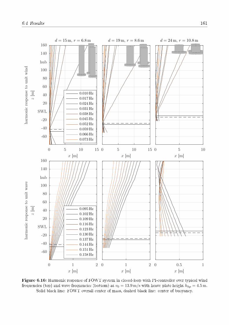
6.4 Results 161
PSfrag replacements
0.095Hz
0.102Hz
0.109Hz
0.116Hz
0.123Hz
0.130Hz
0.137Hz
0.144Hz
0.151Hz
0.158Hz
0.010Hz
0.017Hz
0.024Hz
0.031Hz
0.038Hz
0.045Hz
0.052Hz
0.059Hz
0.066Hz
0.073Hz
d = 24m, r = 10.8md = 19m, r = 8.6md = 15m, r = 6.8m
x [m]
x [m]
x [m]
x [m]
x [m]
har
mon
icre
spon
seto
unit
wav
e
z[m
]
x [m]
har
mon
icre
spon
seto
unit
win
d
z[m
]
0 0.5 1
0 5 10
0 1 2
0 5 10 15
0 1 2
0 5 10 15
-60
-40
-20
SWL
20
40
60
80
100
hub
140
160
-60
-40
-20
SWL
20
40
60
80
100
hub
140
160
Figure 6.16: Harmonic response of FOWT system in closed-loop with PI-controller over typical windfrequencies (top) and wave frequencies (bottom) at v0 = 13.9 m/s with heave plate height hhp = 4.5 m.
Solid black line: FOWT overall center of mass, dashed black line: center of buoyancy.

162 6 Integrated Optimization
Figure 6.16 is also of importance for the design of more advanced controllers as it reveals that
feeding back the platform pitch angle for motion damping might not be harmful for the designs
of deeper drafts, but it would even increase the response of the hub for the low-drafted platform.
In summary, the good performance of the low-draft platform in terms of the DLC 1.2 results
can be explained by the counter-phase pitch response. As the standard RAO to the plat-
form DoFs predicts only the response magnitude in the individual DoFs, it cannot reproduce
this coupled system response behavior, as opposed to the SLOW model used to generate the
harmonic response of Figure 6.16.
Minimum required actuation with perfect control
It has been shown that the harmonic response to waves is a suitable design criterion to predict
the good dynamics of the low-draft shape. In this section, a new design indicator will be
introduced. It quanties the necessary controller activity to reject the external forcing from
wind and waves. The smaller the controller activity, the better the capability of the design to
reject disturbances itself. Figure 6.17 shows the FOWT systemG(jω) with additive disturbance
transfer functions for the same inputs u = [Mg, θ]T and outputs y = [Ω, xt]
T as in Section 3.8.
The disturbance transfer function for wind Gd,v0(jω) and for waves Gd,ζ(jω), collected in Gd,
are again scaled according to Eq. (5.2) as well as the plant G(jω) and the maximum input
magnitude exceeds its limit if ui ≥ 1. According to [259], the minimum required control input
magnitude U∗min for perfect control (perfectly rejecting the disturbances) can be calculated by
solving
U∗min = maxd
(minu‖u‖) s.t. Gu+Gdd = 0; ‖d‖ ≤ 1. (6.2)
with the 2-norm of the inputs ‖u‖2 =√u2
1 + u22 + . . .+ u2
n. Thus, the outputs y as responses
to |d‖ ≤ 1 shall be exactly zero. The required control input u can be obtained given a
disturbance d through system inversion as
u = −G−1Gdd. (6.3)
In order to simplify the problem set of Eq. (6.2), only one disturbance at a time will be
considered in the following: Using the singular values of Eq. (5.3), we can obtain the strongest
and weakest combination of the inputs u. Then, the required control input can be calculated
to cancel the disturbances for both, the strongest and weakest singular values resulting in a
range of the 2-norm of the input signal ‖u‖ in-between these two boundaries according to [259]
as‖Gd‖2
σ(G)≤ ‖u‖2 ≤
‖Gd‖2
σ(G). (6.4)
The resulting system inputs u (the outputs of the inverted system) are the ones necessary to

6.4 Results 163
θ
v0
G(s)
ΩMg
ζ0
xt
Gd,v0(s) Gd,ζ0(s)
Figure 6.17: FOWT square plant with additive disturbances.
perfectly cancel the disturbances. The strongest actuation direction given by the SVD, see
Section 5.1, will be used in the following. Thus, a scalar value of U∗min = ‖Gd‖2/σ(G) results,
representative of both control inputs.
The minimum required actuation U∗min(ω) has been calculated for the dierent platforms, for
wind excitation d = v0 = 1 and wave excitation d = ζ0 = 1, separately in Figure 6.18. The part
from wind excitation (upper part of Figure 6.18) does not show a large variation over the design
space, except for the variation of the eigenfrequencies. For the part from wave excitation it is
dierent: The best performance (equal to the least required actuation U∗min) results here for the
largest column spacing d = 24 m. This is opposite to the RAO of Figure 6.14, which showed
a larger response in pitch for the low-draft platform (d = 24 m) than the narrower (d = 23 m)
design.
Thus, the assessment of the minimum required control input makes it possible to identify
the optimality of the semi-submersibles seen in the harmonic response of Figure 6.16 and the
weighted results of DLC 1.2, Figure 6.9. As opposed to the RAO, U∗min is a design indicator
able to predict the optimal behavior through the counter-phase pitch response.
In summary, this section provided insight into the physical reasons of the low-draft platform
better performing than the ones of deeper draft. The coupled response behavior to waves, with
the surge and pitch-DoF being out of phase giving an almost stationary hub, yields the least
variation of the rotor speed and power and also the smallest tower-base bending. Although this
optimality cannot be seen from the RAO, the new design indicator of the minimum required
control input proves to be better suited here.
The next section will analyze the delity of the reduced-order models compared to FAST for
the three selected designs.

164 6 Integrated Optimization
frequency [Hz]
wav
es:d=
ζ 0
U∗ min(jω)
[-]
win
d:d=
v 0
U∗ min(jω)
[-]
0 0.05 0.1 0.15 0.2 0.25 0.3
0
1
2
3
4
5
0.3
0.4
0.5
0.6
0.7
Figure 6.18: Minimum required control input magnitude U∗min to perfectly reject wind (top) andwave (bottom) disturbances assuming the strongest combination of control inputs u = [Mg, θ] for
platforms of dierent column spacings d = [15(1)24] m (increasing darkness) and hhp = 4.5 m.
6.4.5 Assessment of numerical models for three concepts
The agreement of the reduced-order SLOW models against FAST was shown in Section 3.9 for
the TripleSpar concept at the wind speed bin of vhub = 17.9 m/s. In this section, the code-to-
code comparison will be made for the three dierent designs of the integrated optimization. The
previous analysis showed that the motion response characteristics depend signicantly on the
hull shape of the designs of Figure 6.3. Therefore, the comparison will show if the optimization
results are valid for the entire range of platforms. The following Figures 6.196.23 compare
the response PSD of various signals to the wind and wave excitations, shown on top, between
the reduced-order linearized frequency-domain model, the reduced-order nonlinear time-domain
model and the FAST model.
Model settings
The FAST model has all 25 DoFs enabled, while the SLOW models have 6DoFs and the
motion is only allowed in the vertical xz-plane, see Section 3.2. Radiation damping is neglected
for the reduced-order models, following the argumentation of Sections 3.5.1 and 3.10. The
importance of radiation damping over the design space will be discussed in Section 6.4.6. The
hydrodynamic forces include for all models rst and second-order excitations using Newman's
6.4 Results 165
approximation, see Section 2.5.3, and additionally the drag-induced damping and excitation
from Morison's equation, see Section 3.5.4. All models use the PI-controller with the gains
of Figure 6.4. The below-rated controllers are the same for all models, see Chapter 5, with a
linearized representation of the nonlinear state-feedback in the frequency-domain model.
The results are shown for operational conditions at three wind speeds of Table 2.1 below
rated, above rated and at cut-out: vhub = [7.1, 17.9, 25] m/s. The severity of the sea state does
signicantly increase with the wind speed and thus, the validity of the linearized model is
clearly challenged for the higher waves as nonlinear eects become important. All time-domain
simulations are run over T = 3600 s. A convergence study has been performed with simulation
lengths up to 3 hours, showing that the selected simulation length is enough to obtain reliable
responses in the low-frequency range.
Response spectra to stochastic loads during operation
Figures 6.196.21 show the results for the deep-draft design at the three wind speeds. The
rotor-eective wind speed on top with rotational sampling of turbulence shows a peak at the 3p-
frequency, which has the purpose of introducing the nodding forces through vertical wind
shear. Generally, a good agreement between the reduced-order models and FAST can be
observed. Dierences to FAST are the surge-response at the platform pitch-eigenfrequency at
around 0.03 Hz. The closed loop eigenfrequencies for all platforms were shown in Figure 6.8.
Simulations without aerodynamic forcing have shown that this is due to the aerodynamic
model, while the dierence-frequency forcing is equal between FAST and the reduced model.
This dierence will be discussed more in detail in Section 6.4.6.
The heave response agrees well and is very small compared to the low-draft designs, which
have larger vertical Froude-Krylov forces due to the vertical surfaces closer to SWL. The pitch-
response agrees also well with dierences to FAST again at the pitch-eigenfrequency. For
the small wave height there is no visible response of pitch to waves. This is dierent for
the tower-top displacement xt, which is underpredicted in the wave frequency-range by the
reduced-order models. This is the eect of the neglected radiation damping. It will be seen in
Figure 6.25 (lower left), discussed in Section 6.4.6, for the same platform and same loads that
the simplied constant matrix approach (Section 3.5.1) can result in a larger xt-response with
the radiation model than without.
The response of the rotor speed Ω to low-frequency wind-excitations and to the wave
excitations agrees well among the models, in the same way as the electrical power P . The
section forces at the tower-base have the most energy at the wind frequencies for the small
sea state here. The agreement is very well. Here, no notable dierence occurs between the
linearized and the nonlinear reduced model.

166 6 Integrated Optimization
PSfrag replacements
SLOW linear
SLOW nonlinear
FAST
frequency [Hz]
twr-
ben
dM
yt
[GN
m2/H
z]
pow
erP
[MW
2/H
z]
rot-
spdΩ
[rpm
2/H
z]
twr-
topxt
[m2/H
z]
pit
chβp
[deg
2/H
z]
hea
vez p
[m2/H
z]
surg
exp
[m2/H
z]
wav
eζ 0
[m2/H
z]
win
dv 0
[m2/s
2/H
z]
0.05 0.1 0.15 0.2 0.25 0.3 0.35 0.4 0.45 0.5
0
0.050
5
100
10
200
0.05
0
10
20
300
0.02
0.040
2
40
1
2
0
5
10
Figure 6.19: Model comparison vhub = 7.1 m/s, Hs = 1.7 m, Tp = 8.0 s for deep draft d = 15 m: linearmodel, frequency-domain (blue), nonlinear model, time-domain (red), FAST, time-domain (green).
6.4 Results 167
For the wind speed vhub = 17.9 m/s above rated, Figure 6.20 shows for the deep-draft platform
generally better agreements between the reduced-order models and FAST. The responses to
waves are now clearly larger than for the below-rated case. However, the energy contained in
the low-frequency response of the platform-DoFs (xp, zp, βp) to wind and dierence-frequency
forces is still signicant, compared to the one of rst-order waves. For zp, some scatter of the
heave response magnitude and frequency is visible, which can be due to numerics, considering
the small overall response magnitude in heave. The dierence of xt in the wave frequency
range, due to the neglected radiation damping, is here not as pronounced anymore as in the
smaller sea state. This is because the viscous Morison damping becomes more important than
the linear radiation damping for larger response magnitudes.
Figure 6.21 shows the highest wind speed and the largest sea state with the deep-draft
platform. Here, a large response to rst-order wave forces and a pronounced peak for the
platform pitch eigenfrequency is visible. The agreement of the models is here surprisingly good
as the environmental conditions might suggest that the assumptions for the linearized model
do not hold anymore. The wave response of the rotor speed Ω and the electrical power P
is underpredicted by the linearized model, equally to the following cases. This was discussed
already in Section 3.2.7. A likely reason is the neglect of the cross-correlation between the
rotor-eective wind v0 and the wave height ζ0.
In summary, the code-to-code comparison for the deep-draft platform shows that the SLOW
models can well represent the main resonances at the eigenfrequencies but also the forced
responses to wind, including the 3p-forcing from the wind shear and the response to rst-order
and second-order wave forces. For this deep-draft platform, the hydrodynamic drag at the
columns is more important than for the ones of larger diameter as shown in Figure 2.4. Its
linearization is successful, which is proven by the agreement of the rst-order wave response
and the platform low-frequency resonances.
For the medium-draft and the low-draft designs only the largest sea state is shown here,
while the other two conditions are shown in Appendix B.4. Figure 6.22 shows the medium-
draft design response with t = 50 m at the cut-out wind speed of vhub = 25 m/s. It has generally
a comparable level of agreement among the models as the low-draft design. The only dierence
of the linearized model is the response at the platform pitch mode, which is larger for the
frequency-domain model. As the response for the time-domain models is equal, it is likely
that the linearization is the origin of this dierence. A simple explanation is the dierent
resolution of the frequency-axis for the frequency-domain calculation, which better resolves
this narrow-banded resonance. Another explanation is the linearization technique of the viscous
drag of Section 3.5.4: The selected linearization technique of the Morison damping neglects the
wave kinematics. This does, however, not explain why the agreement is better for the low-
draft platform. The underpredicted rotor speed and power by the linearized model is, again,
attributed to the neglected cross-correlation between the wind and the wave response.

168 6 Integrated Optimization
frequency [Hz]
twr-
ben
dM
yt
[GN
m2/H
z]
pow
erP
[MW
2/H
z]
rot-
spdΩ
[rpm
2/H
z]
bld
ptc
h(θ
)
[deg
2/H
z]
twr-
topxt
[m2/H
z]
pit
chβp
[deg
2/H
z]
hea
vez p
[m2/H
z]
surg
exp
[m2/H
z]
wav
eζ 0
[m2/H
z]
win
dv 0
[m2/s
2/H
z]
0.05 0.1 0.15 0.2 0.25 0.3 0.35 0.4 0.45 0.5
0
0.1
0.2
0
10
20
300
5
0
100
2000
1
20
200
4000
0.1
0.20
200
4000
10
20
300
50
Figure 6.20: Model comparison vhub = 17.9 m/s, Hs = 4.3 m, Tp = 10.0 s for deep draft d = 15 m: lin-ear model, frequency-domain (blue), nonlinear model, time-domain (red), FAST, time-domain (green).
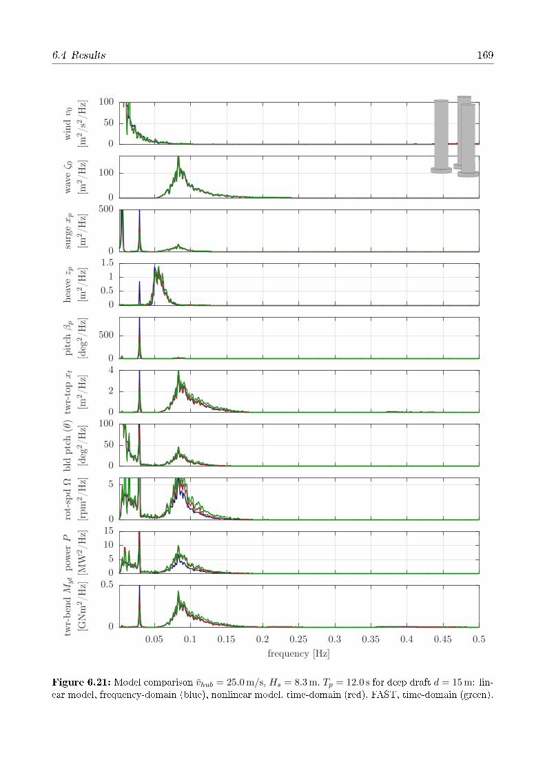
6.4 Results 169
frequency [Hz]
twr-
ben
dM
yt
[GN
m2/H
z]
pow
erP
[MW
2/H
z]
rot-
spdΩ
[rpm
2/H
z]
bld
ptc
h(θ
)
[deg
2/H
z]
twr-
topxt
[m2/H
z]
pit
chβp
[deg
2/H
z]
hea
vez p
[m2/H
z]
surg
exp
[m2/H
z]
wav
eζ 0
[m2/H
z]
win
dv 0
[m2/s
2/H
z]
0.05 0.1 0.15 0.2 0.25 0.3 0.35 0.4 0.45 0.5
0
0.50
5
10
150
5
0
50
1000
2
40
500
0
0.5
1
1.50
5000
100
0
50
100
Figure 6.21: Model comparison vhub = 25.0 m/s, Hs = 8.3 m, Tp = 12.0 s for deep draft d = 15 m: lin-ear model, frequency-domain (blue), nonlinear model, time-domain (red), FAST, time-domain (green).

170 6 Integrated Optimization
frequency [Hz]
twr-
ben
dM
yt
[GN
m2/H
z]
pow
erP
[MW
2/H
z]
rot-
spdΩ
[rpm
2/H
z]
bld
ptc
h(θ
)
[deg
2/H
z]
twr-
topxt
[m2/H
z]
pit
chβp
[deg
2/H
z]
hea
vez p
[m2/H
z]
surg
exp
[m2/H
z]
wav
eζ 0
[m2/H
z]
win
dv 0
[m2/s
2/H
z]
0.05 0.1 0.15 0.2 0.25 0.3 0.35 0.4 0.45 0.5
0
0.1
0.2
0
5
0
1
2
0
50
0
1
2
30
100
0
5
100
50
0
100
0
50
100
Figure 6.22: Model comparison vhub = 25.0 m/s,Hs = 8.3 m, Tp = 12.0 s, medium draft d = 19 m: lin-ear model, frequency-domain (blue), nonlinear model, time-domain (red), FAST, time-domain (green).
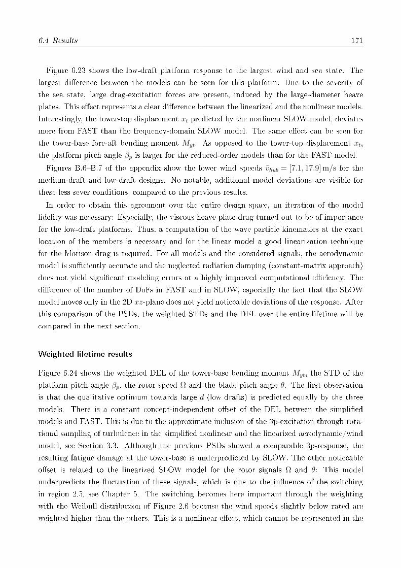
6.4 Results 171
Figure 6.23 shows the low-draft platform response to the largest wind and sea state. The
largest dierence between the models can be seen for this platform: Due to the severity of
the sea state, large drag-excitation forces are present, induced by the large-diameter heave
plates. This eect represents a clear dierence between the linearized and the nonlinear models.
Interestingly, the tower-top displacement xt predicted by the nonlinear SLOW model, deviates
more from FAST than the frequency-domain SLOW model. The same eect can be seen for
the tower-base fore-aft bending moment Myt. As opposed to the tower-top displacement xt,
the platform pitch angle βp is larger for the reduced-order models than for the FAST model.
Figures B.6B.7 of the appendix show the lower wind speeds vhub = [7.1, 17.9] m/s for the
medium-draft and low-draft designs. No notable, additional model deviations are visible for
these less sever conditions, compared to the previous results.
In order to obtain this agreement over the entire design space, an iteration of the model
delity was necessary: Especially, the viscous heave plate drag turned out to be of importance
for the low-draft platforms. Thus, a computation of the wave particle kinematics at the exact
location of the members is necessary and for the linear model a good linearization technique
for the Morison drag is required. For all models and the considered signals, the aerodynamic
model is suciently accurate and the neglected radiation damping (constant-matrix approach)
does not yield signicant modeling errors at a highly improved computational eciency. The
dierence of the number of DoFs in FAST and in SLOW, especially the fact that the SLOW
model moves only in the 2D xz-plane does not yield noticeable deviations of the response. After
this comparison of the PSDs, the weighted STDs and the DEL over the entire lifetime will be
compared in the next section.
Weighted lifetime results
Figure 6.24 shows the weighted DEL of the tower-base bending moment Myt, the STD of the
platform pitch angle βp, the rotor speed Ω and the blade pitch angle θ. The rst observation
is that the qualitative optimum towards large d (low drafts) is predicted equally by the three
models. There is a constant concept-independent oset of the DEL between the simplied
models and FAST. This is due to the approximate inclusion of the 3p-excitation through rota-
tional sampling of turbulence in the simplied nonlinear and the linearized aerodynamic/wind
model, see Section 3.3. Although the previous PSDs showed a comparable 3p-response, the
resulting fatigue damage at the tower-base is underpredicted by SLOW. The other noticeable
oset is related to the linearized SLOW model for the rotor signals Ω and θ: This model
underpredicts the uctuation of these signals, which is due to the inuence of the switching
in region 2.5, see Chapter 5. The switching becomes here important through the weighting
with the Weibull distribution of Figure 2.6 because the wind speeds slightly below rated are
weighted higher than the others. This is a nonlinear eect, which cannot be represented in the
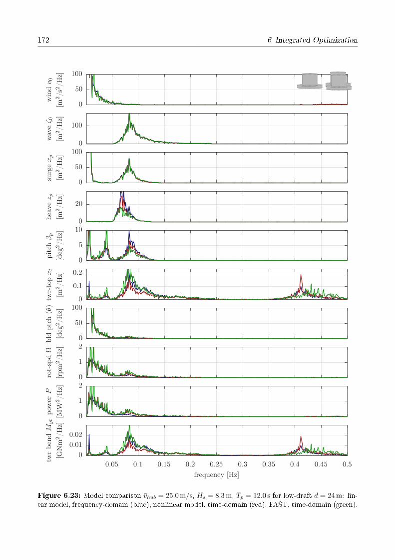
172 6 Integrated Optimization
frequency [Hz]
twr
ben
dM
yt
[GN
m2/H
z]
pow
erP
[MW
2/H
z]
rot-
spdΩ
[rpm
2/H
z]
bld
ptc
h(θ
)
[deg
2/H
z]
twr-
topxt
[m2/H
z]
pit
chβp
[deg
2/H
z]
hea
vez p
[m2/H
z]
surg
exp
[m2/H
z]
wav
eζ 0
[m2/H
z]
win
dv 0
[m2/s
2/H
z]
0.05 0.1 0.15 0.2 0.25 0.3 0.35 0.4 0.45 0.5
0
0.01
0.02
0
1
20
1
20
50
1000
0.1
0.2
0
5
100
20
0
50
1000
100
0
50
100
Figure 6.23: Model comparison vhub = 25.0 m/s, Hs = 8.3 m, Tp = 12.0 s for low-draft d = 24 m: lin-ear model, frequency-domain (blue), nonlinear model, time-domain (red), FAST, time-domain (green).
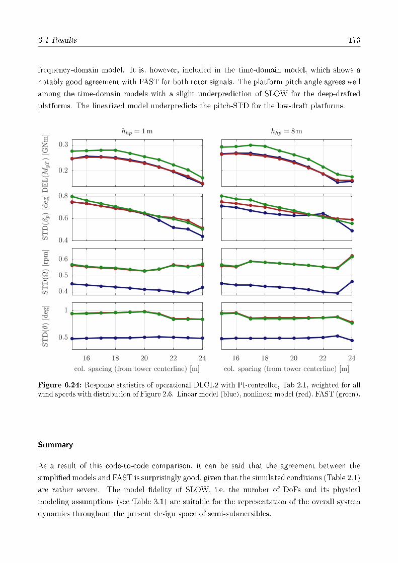
6.4 Results 173
frequency-domain model. It is, however, included in the time-domain model, which shows a
notably good agreement with FAST for both rotor signals. The platform pitch angle agrees well
among the time-domain models with a slight underprediction of SLOW for the deep-drafted
platforms. The linearized model underpredicts the pitch-STD for the low-draft platforms.
PSfrag replacements
hhp = 8mhhp = 1m
col. spacing (from tower centerline) [m]col. spacing (from tower centerline) [m]
ST
D(θ
)[d
eg]
ST
D(Ω
)[r
pm]
ST
D(β
p)[d
eg]D
EL(M
yT)[G
Nm]
16 18 20 22 2416 18 20 22 24
0.5
1
0.4
0.5
0.6
0.4
0.6
0.8
0.2
0.3
Figure 6.24: Response statistics of operational DLC1.2 with PI-controller, Tab 2.1, weighted for allwind speeds with distribution of Figure 2.6. Linear model (blue), nonlinear model (red), FAST (green).
Summary
As a result of this code-to-code comparison, it can be said that the agreement between the
simplied models and FAST is surprisingly good, given that the simulated conditions (Table 2.1)
are rather severe. The model delity of SLOW, i.e. the number of DoFs and its physical
modeling assumptions (see Table 3.1) are suitable for the representation of the overall system
dynamics throughout the present design space of semi-submersibles.

174 6 Integrated Optimization
6.4.6 Model delity
In this section, specic phenomena found in the previous section are analyzed more in detail.
The rst assessment addresses the signicant simplication of SLOW, neglecting the radiation
damping and modeling the radiation memory eect with a constant added mass as introduced
in Section 3.5.1. Also the importance of drag-induced Morison excitation and the eect of
dierence-frequency wave forces is assessed. Finally, the impact of the aerodynamic model on
the pitch-mode below rated is addressed.
Radiation model
The constant-matrix approach is used throughout the analyses of this chapter because it has
clear advantages in terms of computational speed as shown in Table 3.2. However, the simplied
frequency-domain model has the capability to model the radiation memory eect and therefore
simulations have been performed with this model and FAST with the full radiation model and
with the simplied constant matrix approach for both models. It is noted that this approach
does not only impact the damping properties but also the added mass. Consequently, the
constant-matrix approach can have an eect on the system eigenfrequencies.
In order to implement this approximation in FAST, modied Wamit les (.1-le) were gener-
ated with a constant added mass, interpolated at the respective eigenfrequencies, see Figure 3.3.
The radiation damping coecients were set to zero and the ag to compute the radiation
memory eect convolution was switched o. Figure 6.25 shows the comparison between the
linearized SLOW and the FAST model for the deep-draft platform and Figure 6.26 shows the
results for the low-draft platform, both for the below-rated and the cut-out wind speed. All
gures are zoomed in at the frequencies where radiation is important, roughly at the frequen-
cies of the wave spectra, see Figure 3.4. It is noted that the absolute response magnitude is
small in some cases, especially for the below-rated wind speed. In Figure 6.25, it can be seen
for the below-rated wind at vhub = 7.1 m/s that generally, the dierence between the models is
larger than the dierence induced by the radiation eect and the response to rst-order wave
forces is very small. For the cut-out wind at vhub = 25 m/s, FAST does not show any dierence
between the radiation modeling approaches whereas the reduced model shows a slightly smaller
platform response. For the tower-top displacement xt the same holds, whereas the reduced
frequency-domain model gives a smaller response with radiation damping.
Looking now at the same analysis for the low-draft platform in Figure 6.26, the platform
responses for xp and βp for the below-rated wind speed are comparable. For the higher wind
speed (right column), there is a general dierence between SLOW and FAST, with SLOW
predicting a larger response. However, both show a reduced βp response with radiation damping.
This is not the case for the tower-top displacement xt. It shows an even larger response at the
higher wind speed for the low-draft platform with radiation damping enabled compared to the
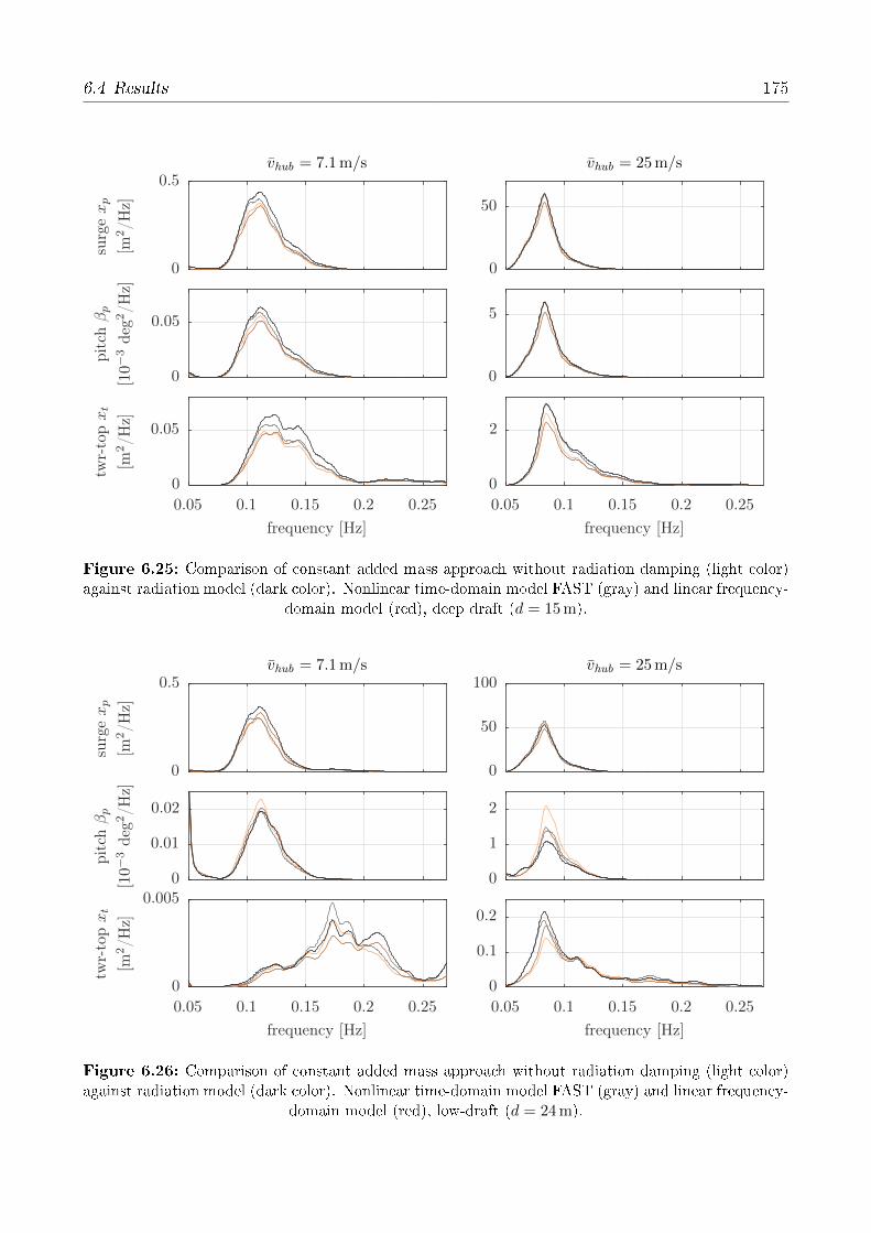
6.4 Results 175
PSfrag replacements
vhub = 25m/svhub = 7.1m/s
frequency [Hz]frequency [Hz]
twr-
topxt
[m2/H
z]
pit
chβp
[10−
3deg
2/H
z]
surg
exp
[m2/H
z]
0.05 0.1 0.15 0.2 0.250.05 0.1 0.15 0.2 0.25
0
2
0
5
0
50
0
0.05
0
0.05
0
0.5
Figure 6.25: Comparison of constant added mass approach without radiation damping (light color)against radiation model (dark color). Nonlinear time-domain model FAST (gray) and linear frequency-
domain model (red), deep draft (d = 15 m).
PSfrag replacements
vhub = 25m/svhub = 7.1m/s
frequency [Hz]frequency [Hz]
twr-
topxt
[m2/H
z]
pit
chβp
[10−
3deg
2/H
z]
surg
exp
[m2/H
z]
0.05 0.1 0.15 0.2 0.250.05 0.1 0.15 0.2 0.25
0
0.1
0.2
0
1
2
0
50
100
0
0.0050
0.01
0.02
0
0.5
Figure 6.26: Comparison of constant added mass approach without radiation damping (light color)against radiation model (dark color). Nonlinear time-domain model FAST (gray) and linear frequency-
domain model (red), low-draft (d = 24 m).
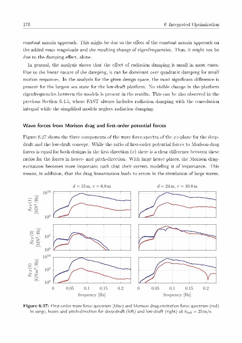
176 6 Integrated Optimization
constant matrix approach. This might be due to the eect of the constant matrix approach on
the added mass magnitude and the resulting change of eigenfrequencies. Thus, it might not be
due to the damping eect, alone.
In general, the analysis shows that the eect of radiation damping is small in most cases.
Due to the linear nature of the damping, it can be dominant over quadratic damping for small
motion responses. In the analysis for the given design space, the most signicant dierence is
present for the largest sea state for the low-draft platform. No visible change in the platform
eigenfrequencies between the models is present in the results. This can be also observed in the
previous Section 6.4.5, where FAST always includes radiation damping with the convolution
integral while the simplied models neglect radiation damping.
Wave forces from Morison drag and rst-order potential forces
Figure 6.27 shows the three components of the wave force spectra of the xz-plane for the deep-
draft and the low-draft concept. While the ratio of rst-order potential forces to Morison-drag
forces is equal for both designs in the rst direction (x) there is a clear dierence between these
ratios for the forces in heave- and pitch-direction. With large heave plates, the Morison drag-
excitation becomes more important such that their correct modeling is of importance. This
means, in addition, that the drag linearization leads to errors in the simulation of large waves.
d = 24m, r = 10.8md = 15m, r = 6.8m
frequency [Hz]frequency [Hz]
SFF(5)
[GN
m2/H
z]SFF(3)
[MN
2/H
z]
SFF(1)
[MN
2/H
z]
0 0.05 0.1 0.15 0.20 0.05 0.1 0.15 0.2
100
105
1010100
105
100
1010
Figure 6.27: First-order wave force spectrum (blue) and Morison drag-excitation force spectrum (red)in surge, heave and pitch-direction for deep-draft (left) and low-draft (right) at vhub = 25 m/s.
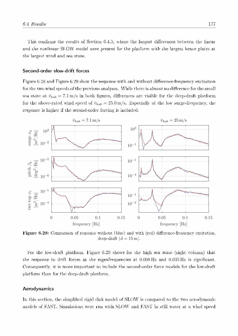
6.4 Results 177
This conrms the results of Section 6.4.5, where the largest dierences between the linear
and the nonlinear SLOW model were present for the platform with the largest heave plates at
the largest wind and sea state.
Second-order slow-drift forces
Figure 6.28 and Figure 6.29 show the response with and without dierence-frequency excitation
for the two wind speeds of the previous analyses. While there is almost no dierence for the small
sea state at vhub = 7.1 m/s in both gures, dierences are visible for the deep-draft platform
for the above-rated wind speed of vhub = 25.0 m/s. Especially at the low surge-frequency, the
response is higher if the second-order forcing is included.
PSfrag replacements
vhub = 25m/svhub = 7.1m/s
frequency [Hz]frequency [Hz]
twr-
topxt
[m2/H
z]
pit
chβp
[deg
2/H
z]
surg
exp
[m2/H
z]
0 0.05 0.1 0.150 0.05 0.1 0.15
10−3
10−1
10−4
10−1
10−1
103
10−4
10−1
10−6
10−2
10−2
102
Figure 6.28: Comparison of response without (blue) and with (red) dierence-frequency excitation,deep-draft (d = 15 m).
For the low-draft platform, Figure 6.29 shows for the high sea state (right column) that
the response to drift forces at the eigenfrequencies at 0.008 Hz and 0.035 Hz is signicant.
Consequently, it is more important to include the second-order force models for the low-draft
platform than for the deep-draft platform.
Aerodynamics
In this section, the simplied rigid disk model of SLOW is compared to the two aerodynamic
models of FAST. Simulations were run with SLOW and FAST in still water at a wind speed
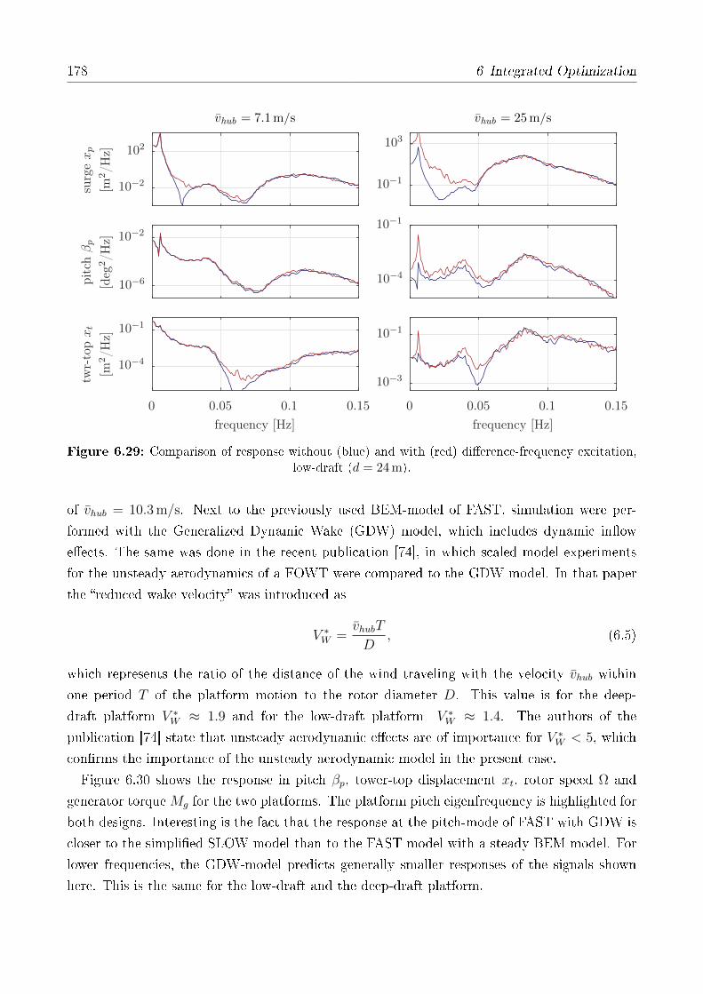
178 6 Integrated Optimization
PSfrag replacements
vhub = 25m/svhub = 7.1m/s
frequency [Hz]frequency [Hz]
twr-
topxt
[m2/H
z]
pit
chβp
[deg
2/H
z]
surg
exp
[m2/H
z]
0 0.05 0.1 0.150 0.05 0.1 0.15
10−3
10−1
10−4
10−1
10−1
103
10−4
10−1
10−6
10−2
10−2
102
Figure 6.29: Comparison of response without (blue) and with (red) dierence-frequency excitation,low-draft (d = 24 m).
of vhub = 10.3 m/s. Next to the previously used BEM-model of FAST, simulation were per-
formed with the Generalized Dynamic Wake (GDW) model, which includes dynamic inow
eects. The same was done in the recent publication [74], in which scaled model experiments
for the unsteady aerodynamics of a FOWT were compared to the GDW model. In that paper
the reduced wake velocity was introduced as
V ∗W =vhubT
D, (6.5)
which represents the ratio of the distance of the wind traveling with the velocity vhub within
one period T of the platform motion to the rotor diameter D. This value is for the deep-
draft platform V ∗W ≈ 1.9 and for the low-draft platform V ∗W ≈ 1.4. The authors of the
publication [74] state that unsteady aerodynamic eects are of importance for V ∗W < 5, which
conrms the importance of the unsteady aerodynamic model in the present case.
Figure 6.30 shows the response in pitch βp, tower-top displacement xt, rotor speed Ω and
generator torqueMg for the two platforms. The platform pitch eigenfrequency is highlighted for
both designs. Interesting is the fact that the response at the pitch-mode of FAST with GDW is
closer to the simplied SLOW model than to the FAST model with a steady BEM model. For
lower frequencies, the GDW-model predicts generally smaller responses of the signals shown
here. This is the same for the low-draft and the deep-draft platform.
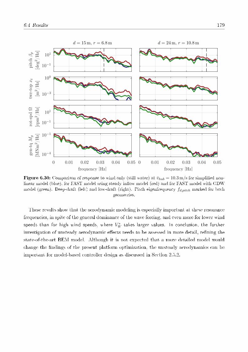
6.4 Results 179
PSfrag replacements
d = 24m, r = 10.8md = 15m, r = 6.8m
frequency [Hz]frequency [Hz]
gen-t
qM
g
[MN
m2/H
z]
rot-
spdΩ
[rpm
2/H
z]
twr-
topxt
[m2/H
z]
pit
chβp
[deg
2/H
z]
0 0.01 0.02 0.03 0.04 0.050 0.01 0.02 0.03 0.04 0.05
10−4
10−1
10−1
101
10−3
100
10−1
101
Figure 6.30: Comparison of response to wind only (still water) at vhub = 10.3 m/s for simplied non-linear model (blue), for FAST model using steady inow model (red) and for FAST model with GDWmodel (green). Deep-draft (left) and low-draft (right). Pitch eigenfrequency fd,pitch marked for both
geometries.
These results show that the aerodynamic modeling is especially important at these resonance
frequencies, in spite of the general dominance of the wave forcing, and even more for lower wind
speeds than for high wind speeds, where V ∗W takes larger values. In conclusion, the further
investigation of unsteady aerodynamic eects needs to be assessed in more detail, rening the
state-of-the-art BEM model. Although it is not expected that a more detailed model would
change the ndings of the present platform optimization, the unsteady aerodynamics can be
important for model-based controller design as discussed in Section 2.5.2.

7 Conclusions and Outlook
The goal of this work was to improve the understanding of how wind and waves impact the dy-
namic behavior of the oating systems and how their shape can be optimized for oating wind
turbines showing the same stable dynamics as bottom-xed ones with a rather lightweight, and
resource-ecient foundation. In order to pursue this goal, a dedicated simulation model was
developed with a simplied representation of the structure, the aerodynamics and hydrodynam-
ics. The developed model was veried with the open-source code FAST for a public baseline
design of a 10 MW turbine on a concrete deep-draft semi-submersible. It was also validated
against scaled experiments of the same concept in a combined wind and wave tank including
blade pitch control. Finally, a brute-force optimization of a three-column semi-submersible
with adapted wind turbine controllers revealed that an optimization of the hull shape can yield
a reduction of the tower-base bending moment of more than 30 %, yielding comparable fatigue
to onshore turbines.
7.1 Reduced-Order Simulation Model
A exible multibody system has been developed with a general formulation that is not specic
to wind turbines. It has been set up with only six degrees of freedom, allowing a motion in two
dimensions. A symbolic linearization method yields a linear representation, which was used for
load calculations in the frequency-domain and linear system analyses. Through a comparison of
the simulation results with the higher-delity FAST code and experimental data, the relevance
of the physical eects could be estimated.
A rather high level of detail was selected for the hydrodynamic model because the loads and
motion response of oating wind turbines is dominated by the wave forcing and the hydrody-
namic viscous drag is important for the overall system dynamics. In addition to the rst-order
panel code coecients, a exible node-based implementation of Morison's equation was real-
ized. The Morison drag forces include the horizontal and vertical components of damping, as
well as wave excitation. The magnitude of the Morison drag-excitation depends strongly on
the semi-submersible heave plates and requires a proper linearization procedure or a nonlinear
modeling for large sea-states. The radiation memory eect, however, has shown to have a
minor impact on the main system dynamics for the considered platform shapes. Its proposed

182 7 Conclusions and Outlook
simplication yields a substantially decreased simulation time. For an identication of the hy-
drodynamic drag coecients, especially the inclusion of the second-order dierence-frequency
forces was important. The results of the model validation led to a parametric denition of the
heave plate drag, which, using the linearized frequency-domain model, allowed for an iterative
solution. These load case-dependent drag coecients were used for the simplied nonlinear
model and the FAST model. Both results show that the parametric heave plate drag results
mainly in larger global damping coecients for larger sea-states. It will be important to take
such a parameterization into account for a realistic estimation of the hydrodynamic damping
in load simulations.
The aerodynamics could be well represented through an ecient force model for the integral
rotor. The quasi-static model provides the rotor forces as function of the tip speed ratio and
the blade pitch angle, the actuated variable of the above-rated controller. For a representation
of the blade excitation from wind shear, rotational sampling of turbulence showed to be an
ecient and suitable method.
In a comparison with FAST, the model has proven to be able to represent the dominant
system dynamics, the main eigenfrequencies but also the magnitude of the frequency response
to rather severe met-ocean conditions. In a comparison against scaled experiments, the eigen-
frequencies and the magnitude of the response to wind and wave forces was well predicted.
The computational performance of the time-domain model is such that a simulation runs
about 120 times faster than real-time. The linear frequency-domain model requires only matrix
algebraic operations and is therefore even faster. Common state-of-the-art simulation models
are usually not faster than twice the real-time, which might limit large conceptual design
studies.
The model was successfully applied for linear model-based controller design. The resulting PI-
controller proved to be suitable also for the FAST model, which includes dynamics, neglected
in the controller design model. The integrated platform optimization over a large design space
of semi-submersible platforms made use of the tailored properties of the model. Although
the hydrodynamic properties of the analyzed platforms show a large variation with dierent
characteristics of the hydrodynamic forcing, the developed model was able to reliably predict
the dynamic behavior for all designs. A verication of the optimization results with FAST
showed the same optimum.
Although the model description, adapted to the problem, is highly ecient for this work,
there are clear limitations, related to the simplications of the above mentioned involved sub-
models. Especially the motion, constrained to the vertical plane in wind and wave direction
prohibits the modeling of yawed inow and misaligned waves. The structural dynamics ne-
glect the elasticity of the oating platform, the higher tower modes and the blade elasticity.
The simplied representation of the aerodynamics does not allow for the simulation of extreme
aerodynamic situation with strong shears, transient events or stalled ow conditions. The hy-
7.2 Controller Design 183
drodynamic model resembles more the one of the FAST model but there is also a restriction to
linear waves and the second-order slow drift forces are approximated. Hence, the model is well
suited for operational conditions without failures or extreme events. Operational load cases are
the important ones in the concept design stage and for a general system optimization. Extreme
cases are subject of the detailed design stage, which requires high-delity models, adapted to
the complexity of the simulated conditions.
In summary, the developed reduced-order simulation model could successfully ll the gap
between spreadsheet calculations on one side and simulation tools for certication on the other
side. It is hence a well-suited model for the conceptual design phase of oating wind systems.
Even though it includes all main system dynamic eects, it can be used for large parameter
studies. It was shown in the integrated optimization that such a coupled description is necessary
to nd the optimum for the herein selected design space of semi-submersible platforms, as
opposed to simpler, de-coupled approaches.
7.2 Controller Design
A Single-Input-Single-Output (SISO)-design procedure was developed, satisfying a predened
stability margin at all operating points. With this new procedure of a gain scheduling controller
for oating wind turbines, the entire system is considered for the controller design. Commonly,
the gain scheduling function maintains the closed loop rotor dynamics over the entire operating
range.
In the proposed method, not only the rotor dynamics but the entire FOWT dynamic system
stability is a design criterion for all operating points. The developed SISO design procedure
yields a gain scheduling for above-rated wind speeds, which diers from the common gain
scheduling of onshore turbines. This is because the stability issue of oating wind turbines is
more critical for lower wind speeds than for higher wind speeds. As a result, the proportional
gain decreases for increasing wind speeds above rated, before it increases again towards cut-out
wind speeds. A rather high time constant of the SISO-Proportional-Integral (PI)-controller
showed to give better results for oating turbines, which is another dierence to common on-
shore controllers. The advantages of this controller are the robustness properties and therefore
the high independence from the simulation model in terms of unmodeled dynamics of the design
model. The developed design algorithm can be automated using the linearized model in each
operating point.
Additionally to this controller, an optimal Multi-Input-Multi-Output (MIMO) controller was
designed, in order to show its advantages over the previous one. The determination of the
controller weights was successful with a good performance over the design space. While the
controller showed to improve signicantly the damping of the system resonances, its robustness
184 7 Conclusions and Outlook
is limited. Therefore, the controller is useful as an indicator of the upper performance bound,
showing the theoretical potential to damp low-frequency platform resonances and improving
rotor speed tracking.
7.3 Integrated Optimization
The optimum platform shape of a concrete semi-submersible was found through an integrated
design approach. The primary goal of this optimization was to improve the overall system
dynamics of the FOWT, such that the response of the system to stochastic wind and wave
loads in fore-aft direction but also in terms of the power uctuation is reduced. To meet this
goal, a small design space of a three-column semi-submersible with heave plates was set up,
ranging from a slender deep-draft geometry to a low-draft one with large column diameter. As a
result of the optimization, the low-drafted design gave a promising improvement of the response
of the tower-base bending, at only slightly higher levels than onshore wind turbines (which are
not subject to wave forcing).
Subsequent analyses using the linear dynamic model revealed the reasons of the variation of
the performance among the dierent designs. The optimum design was found to be not the
one with the smallest wave load amplication in pitch-direction as predicted by the Response
Amplitude Operator (RAO), the commonly used performance indicator in the conceptual design
phase. With the harmonic response function, derived from the developed linearized low-order
model, the dynamic characteristics of the optimum shape could be identied: The FOWT
response amplitudes to unit waves along the tower centerline were visualized. The optimal
design shows almost no fore-aft motion at the rotor hub, which means that the entire system,
subject to wave loads, rotates about this point. As a result, the hub is almost stationary and
the uctuations of the power, the rotor speed, generator torque and blade pitch angle can
be signicantly reduced. An interpretation of this is that the surge and pitch response are
out-of-phase, yielding a positive surge displacement when the pitch angle is negative.
In order to generally rate the suitability of a oating platform to support a wind turbine, a
new performance indicator was developed: From control engineering, controllability measures
are known, quantifying the necessary actuator performance for perfectly rejecting a given dis-
turbance. A plot of this least required actuator action to reject the wave loads showed that
the actuator action magnitude, especially at the wave frequencies, is proportional to the fatigue
loads over the design space. Consequently, this indicator is one which is able to predict the
platform design optimum obtained from the conducted optimization.

7.4 Outlook 185
7.4 Outlook
The reduced-order simulation model SLOW, the parametric control routines, as well as the
integrated optimization approach can be employed in further studies. Tailored designs, grown
into the ocean environment, rejecting wind and wave loads with the help of advanced sensors
and actuators, shall help to make oating wind more sustainable in the future. The following
works, based on the presented thesis, are conceivable:
• Structural model: The blade elasticity was not included in the present work. However,
works started on including modally reduced bodies for the blades and need to be continued
in order to be able to compute the blade loads and represent azimuth-dependent loading
on the rotor.
• Aerodynamic model: A more detailed model including azimuth dependency, aerodynamic
states and sheared inow should be implemented while keeping the eciency. In certain
conditions, unsteady aerodynamic eects can be of importance for model-based controller
design and should be represented.
• Hydrodynamic model: Only one possible way of implementing the linearized Morison
equation was realized. The inuence of the cross-correlation between body motion and
wave motion is to be analyzed as well as other, improved, formulations for the drag
linearization.
• Experiments: The tool validation with scaled experiments showed that the magnitude of
the response to wind and waves and the system dynamic properties are well predicted by
the developed simulation model. However, the uncertainty related to all of the involved
components, measurement devices and testing procedures needs to be assessed. This will
go in line with the further improvement of the testing methodologies themselves, mitigat-
ing the issues related to the simultaneous scaling of aerodynamics and hydrodynamics.
• Control: A standard and an optimal controller were developed. A frequency-domain
optimal controller should be tested, especially for a further reduction of the response to
rst-order wave loads.
• Optimization: The developed methodology can be applied to other concepts of oating
wind turbines. Closed-loop optimization algorithms were tested in this work but not
shown here in order to allow a better interpretation and visualization. The development
of suitable cost functions and the selection of appropriate optimizers should be addressed
using Systems Engineering approaches.


A Model Parameters
All parameters of the FOWT designs used in this work are listed in the following Sections A.1
A.3. Platform parameters always refer to the structural properties of the platform from keel to
the tower base, without mooring lines.
A.1 Full-Scale TripleSpar Parameters
Table A.1 lists the parameters of the scaled simulation model used for the simulations of Chap-
ter 6.
Table A.1: Model parameters of the full-scale TripleSpar concept with the DTU 10 MW RWT.
Parameter Unit Value
Platform mass (incl. ballast) [kg] 2.82682× 10⁷
Tower mass [kg] 4.36451× 10⁵
Nacelle mass [kg] 4.46036× 10⁵
Rotor mass [kg] 2.30598× 10⁵
Platform inertia about y w.r.t. its CM [kgm2] 1.8674× 10¹⁰
Nacelle inertia about y w.r.t. its CM [kgm2] 7.32634× 10⁶
Column spacing (to tower centerline) [m] 26.0
Column diameter [m] 15.0
Heave plate thickness [m] 0.5
Heave plate diameter [m] 22.5
Draft [m] 54.464
Platform CM below SWL [m] 36.018
Tower-base above SWL [m] 25.0
Tower CM above SWL [m] 63.72
Nacelle CM above SWL [m] 118.08
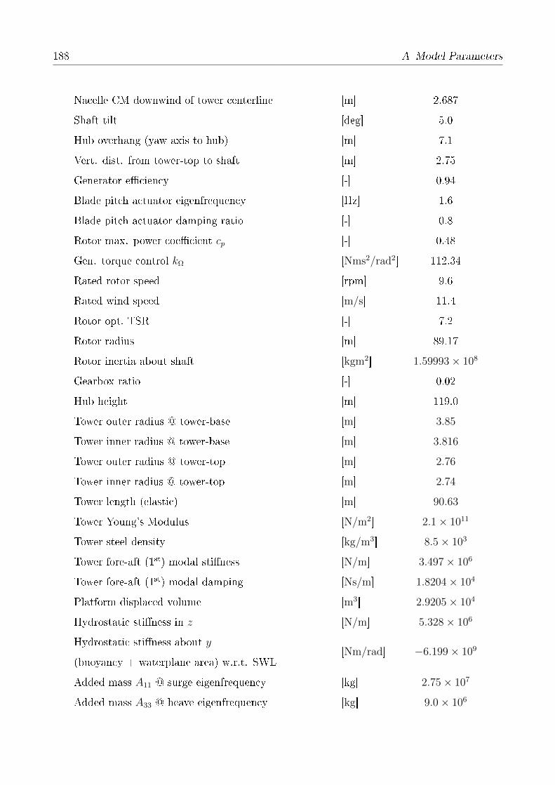
188 A Model Parameters
Nacelle CM downwind of tower centerline [m] 2.687
Shaft tilt [deg] 5.0
Hub overhang (yaw axis to hub) [m] 7.1
Vert. dist. from tower-top to shaft [m] 2.75
Generator eciency [-] 0.94
Blade pitch actuator eigenfrequency [Hz] 1.6
Blade pitch actuator damping ratio [-] 0.8
Rotor max. power coecient cp [-] 0.48
Gen. torque control kΩ [Nms2/rad2] 112.34
Rated rotor speed [rpm] 9.6
Rated wind speed [m/s] 11.4
Rotor opt. TSR [-] 7.2
Rotor radius [m] 89.17
Rotor inertia about shaft [kgm2] 1.59993× 10⁸
Gearbox ratio [-] 0.02
Hub height [m] 119.0
Tower outer radius @ tower-base [m] 3.85
Tower inner radius @ tower-base [m] 3.816
Tower outer radius @ tower-top [m] 2.76
Tower inner radius @ tower-top [m] 2.74
Tower length (elastic) [m] 90.63
Tower Young's Modulus [N/m2] 2.1× 10¹¹
Tower steel density [kg/m3] 8.5× 10³
Tower fore-aft (1st) modal stiness [N/m] 3.497× 10⁶
Tower fore-aft (1st) modal damping [Ns/m] 1.8204× 10⁴
Platform displaced volume [m3] 2.9205× 10⁴
Hydrostatic stiness in z [N/m] 5.328× 10⁶
Hydrostatic stiness about y[Nm/rad] −6.199× 10⁹
(buoyancy + waterplane area) w.r.t. SWL
Added mass A11 @ surge eigenfrequency [kg] 2.75× 10⁷
Added mass A33 @ heave eigenfrequency [kg] 9.0× 10⁶
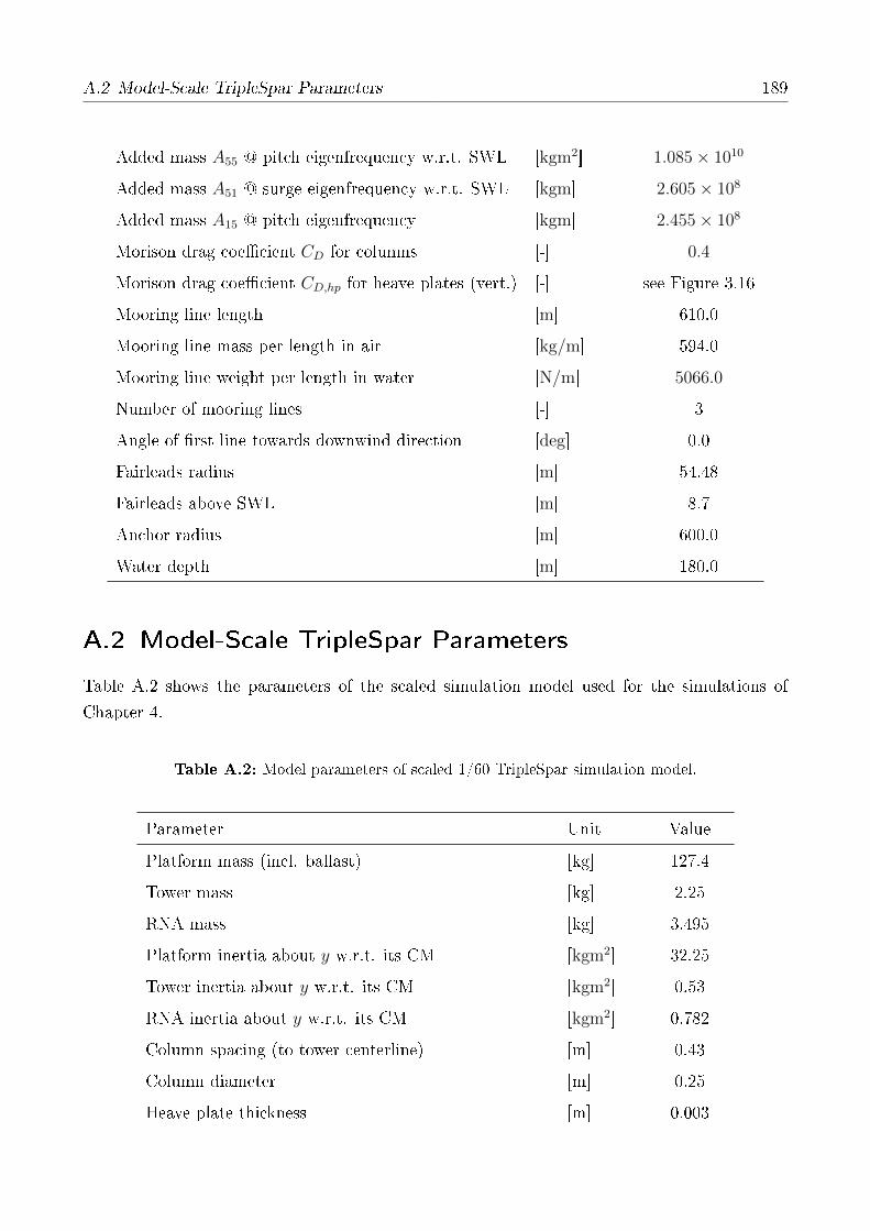
A.2 Model-Scale TripleSpar Parameters 189
Added mass A55 @ pitch eigenfrequency w.r.t. SWL [kgm2] 1.085× 10¹⁰
Added mass A51 @ surge eigenfrequency w.r.t. SWL [kgm] 2.605× 10⁸
Added mass A15 @ pitch eigenfrequency [kgm] 2.455× 10⁸
Morison drag coecient CD for columns [-] 0.4
Morison drag coecient CD,hp for heave plates (vert.) [-] see Figure 3.16
Mooring line length [m] 610.0
Mooring line mass per length in air [kg/m] 594.0
Mooring line weight per length in water [N/m] 5066.0
Number of mooring lines [-] 3
Angle of rst line towards downwind direction [deg] 0.0
Fairleads radius [m] 54.48
Fairleads above SWL [m] 8.7
Anchor radius [m] 600.0
Water depth [m] 180.0
A.2 Model-Scale TripleSpar Parameters
Table A.2 shows the parameters of the scaled simulation model used for the simulations of
Chapter 4.
Table A.2: Model parameters of scaled 1/60 TripleSpar simulation model.
Parameter Unit Value
Platform mass (incl. ballast) [kg] 127.4
Tower mass [kg] 2.25
RNA mass [kg] 3.495
Platform inertia about y w.r.t. its CM [kgm2] 32.25
Tower inertia about y w.r.t. its CM [kgm2] 0.53
RNA inertia about y w.r.t. its CM [kgm2] 0.782
Column spacing (to tower centerline) [m] 0.43
Column diameter [m] 0.25
Heave plate thickness [m] 0.003
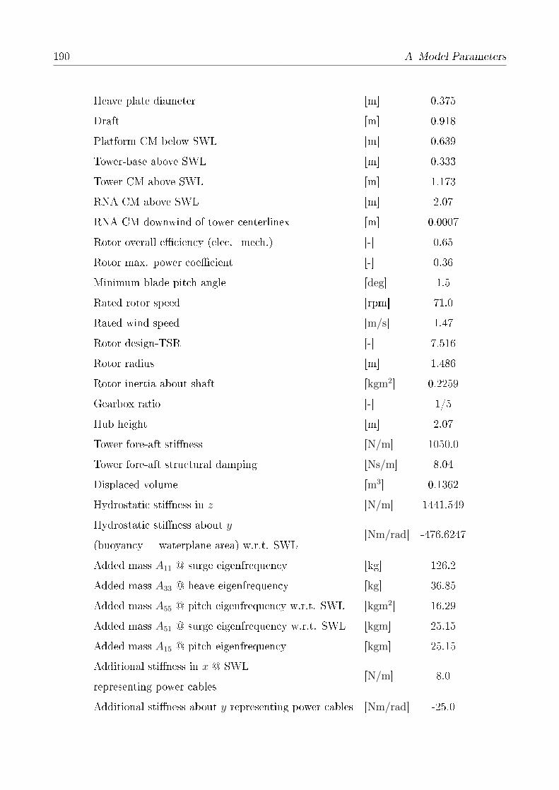
190 A Model Parameters
Heave plate diameter [m] 0.375
Draft [m] 0.918
Platform CM below SWL [m] 0.639
Tower-base above SWL [m] 0.333
Tower CM above SWL [m] 1.173
RNA CM above SWL [m] 2.07
RNA CM downwind of tower centerlinex [m] 0.0007
Rotor overall eciency (elec.+mech.) [-] 0.65
Rotor max. power coecient [-] 0.36
Minimum blade pitch angle [deg] 1.5
Rated rotor speed [rpm] 71.0
Rated wind speed [m/s] 1.47
Rotor design-TSR [-] 7.516
Rotor radius [m] 1.486
Rotor inertia about shaft [kgm2] 0.2259
Gearbox ratio [-] 1/5
Hub height [m] 2.07
Tower fore-aft stiness [N/m] 1050.0
Tower fore-aft structural damping [Ns/m] 8.04
Displaced volume [m3] 0.1362
Hydrostatic stiness in z [N/m] 1441.549
Hydrostatic stiness about y[Nm/rad] -476.6247
(buoyancy + waterplane area) w.r.t. SWL
Added mass A11 @ surge eigenfrequency [kg] 126.2
Added mass A33 @ heave eigenfrequency [kg] 36.85
Added mass A55 @ pitch eigenfrequency w.r.t. SWL [kgm2] 16.29
Added mass A51 @ surge eigenfrequency w.r.t. SWL [kgm] 25.15
Added mass A15 @ pitch eigenfrequency [kgm] 25.15
Additional stiness in x @ SWL[N/m] 8.0
representing power cables
Additional stiness about y representing power cables [Nm/rad] -25.0

A.3 Deep-Draft, Medium-Draft and Low-Draft Parameters 191
Mooring line length [m] 9.95
Mooring line mass per length in air [kg/m] 0.1650
Mooring line weight per length in water [N/m] 1.4072
Number of mooring lines [-] 3
Angle of rst line towards downwind direction [deg] 0.0
Fairleads radius [m] 0.908
Fairleads above SWL [m] 0.145
Anchor radius [m] 9.74
Water depth [m] 3.0
A.3 Deep-Draft, Medium-Draft and Low-Draft
Parameters
Table A.3 shows the parameters of the three selected platforms of the design space of Chapter 6.
All values not included in Table A.3 are equal to the ones of Table A.1.
Table A.3: Model parameters of deep-draft, medium-draft and low-draft platforms.
Parameter Deep-draft Medium-draft Low-draft
Platform mass (incl. ballast) [kg] 36.051× 10⁶ 38.691× 10⁶ 31.149× 10⁶
Platform inertia about y w.r.t. CM [kgm2] 28.38× 10⁹ 17.0× 10⁹ 87.97× 10⁸
Column spacing (to tower centerline) [m] 15.0 19.0 24.0
Column radius [m] 6.76 8.56 10.81
Heave plate thickness [m] 4.5 4.5 4.5
Heave plate radius [m] 10.9 13.8 17.4
Draft [m] 78.48 49.95 21.94
Platform CM below SWL [m] 52.34 34.28 13.36
Displaced volume [m3] 3.6837× 10⁴ 3.9412× 10⁴ 3.2055× 10⁴
Fairleads radius [m] 26.0
Fairleads above SWL [m] 8.7
Anchor radius [m] 571.5


B Additional Results
The results, presented in the following, complete the results of Chapter 6. For the cases, where
not all of the three selected platforms of Table 6.2, or not all of the three wind speeds could be
shown, results can be found in the following sections. An additional sensitivity study, assessing
the eect of the peak spectral wave period is subject of Section B.2.
B.1 Comparison of Controllers for Low-Draft Platform
Figure B.1 shows the PSD for the low-draft platform. It can be seen that the LQR performs
better than the PI-controller also for this platform, as it does for the deep-draft platform,
Figure 6.12. This conrms the validity of the selected LQR gains of Table 5.2.
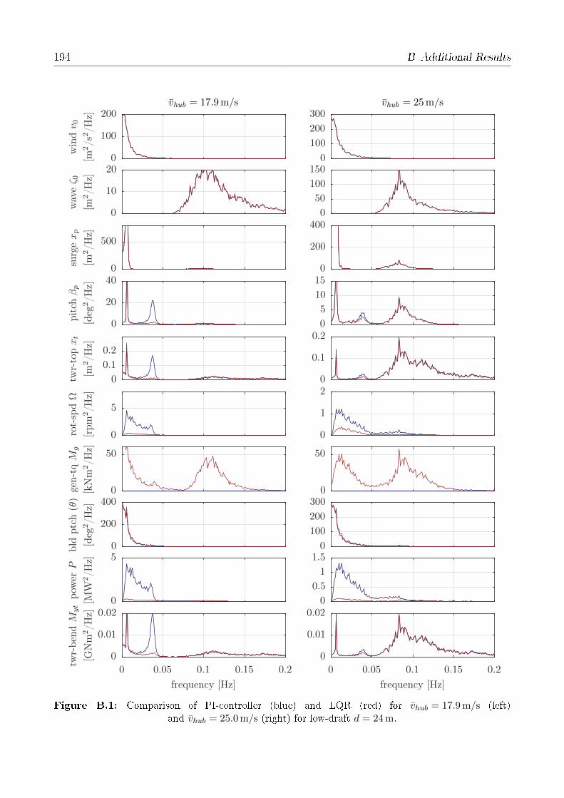
194 B Additional Results
PSfrag replacements
vhub = 25m/svhub = 17.9m/s
frequency [Hz]frequency [Hz]
twr-
ben
dM
yt
[GN
m2/H
z]
pow
erP
[MW
2/H
z]
bld
ptc
h(θ
)
[deg
2/H
z]
gen-t
qM
g
[kN
m2/H
z]
rot-
spdΩ
[rpm
2/H
z]
twr-
topxt
[m2/H
z]
pit
chβp
[deg
2/H
z]
surg
exp
[m2/H
z]
wav
eζ 0
[m2/H
z]
win
dv 0
[m2/s
2/H
z]
0 0.05 0.1 0.15 0.20 0.05 0.1 0.15 0.2
0
0.01
0.020
0.5
1
1.50
100
200
3000
50
0
1
20
0.1
0.20
5
10
150
200
4000
50
100
1500
100
200
300
0
0.01
0.020
50
200
4000
50
0
5
0
0.1
0.2
0
20
400
500
0
10
200
100
200
Figure B.1: Comparison of PI-controller (blue) and LQR (red) for vhub = 17.9 m/s (left)and vhub = 25.0 m/s (right) for low-draft d = 24 m.
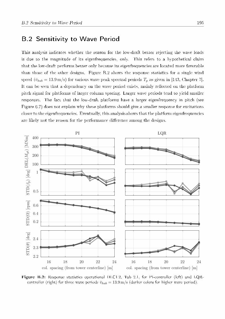
B.2 Sensitivity to Wave Period 195
B.2 Sensitivity to Wave Period
This analysis indicates whether the reason for the low-draft better rejecting the wave loads
is due to the magnitude of its eigenfrequencies, only. This refers to a hypothetical claim
that the low-draft performs better only because its eigenfrequencies are located more favorable
than those of the other designs. Figure B.2 shows the response statistics for a single wind
speed (vhub = 13.9 m/s) for various wave peak spectral periods Tp as given in [143, Chapter 7].
It can be seen that a dependency on the wave period exists, mainly reected on the platform
pitch signal for platforms of larger column spacing. Larger wave periods tend to yield smaller
responses. The fact that the low-draft platforms have a larger eigenfrequency in pitch (see
Figure 6.7) does not explain why these platforms should give a smaller response for excitations
closer to the eigenfrequencies. Eventually, this analysis shows that the platform eigenfrequencies
are likely not the reason for the performance dierence among the designs.
LQRPI
col. spacing (from tower centerline) [m]col. spacing (from tower centerline) [m]
ST
D(θ
)[d
eg]
ST
D(Ω
)[r
pm]
ST
D(β
p)[d
eg]
DE
L(M
yt)
[MN
m]
16 18 20 22 2416 18 20 22 24
2.2
2.3
2.4
0.2
0.4
0.6
0.5
1
100
200
300
400
Figure B.2: Response statistics operational DLC1.2, Tab 2.1, for PI-controller (left) and LQR-controller (right) for three wave periods vhub = 13.9 m/s (darker colors for higher wave period).

196 B Additional Results
B.3 Harmonic Response
Figure B.3 shows the harmonic response for the column spacings d ≤ 24 m. In Figure 6.16 it
could be observed that the instantaneous center of rotation due to sinusoidal wave excitations
moves from positions far below SWL to the hub for the low-draft platform. In Figure B.3 it
can be seen that the transition of the center of rotation happens only for the largest considered
spacing of d = 24 m. For platforms of smaller breadth, the pitch motion is almost completely
suppressed yielding to a surge-motion, only. In fact, this behavior can also yield a good perfor-
mance in terms of tower-sectional loads since no moments due to gravity are present.
PSfrag replacements
0.095Hz
0.102Hz
0.109Hz
0.116Hz
0.123Hz
0.130Hz
0.137Hz
0.144Hz
0.151Hz
0.158Hz
x [m]x [m]x [m]
har
mon
icre
spon
seto
unit
wav
e
z[m
]
0 0.5 10 0.2 0.4 0.60 0.5 1
-60
-40
-20
SWL
20
40
60
80
100
hub
140
160
Figure B.3: Harmonic response for upper range of column spacings (d = [22, 23, 24] m) of FOWTsystem in closed loop with PI-controller over typical wind frequencies (top) and wave frequencies (bot-tom) at v0 = 13.9 m/s with heave plate height hhp = 4.5 m. Solid black line: FOWT overall center of
mass, dashed black line: center of buoyancy. Compare to Figure 6.16.
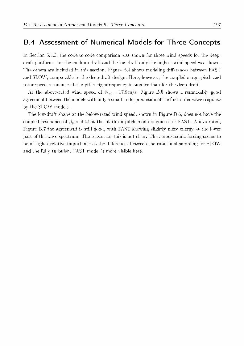
B.4 Assessment of Numerical Models for Three Concepts 197
B.4 Assessment of Numerical Models for Three Concepts
In Section 6.4.5, the code-to-code comparison was shown for three wind speeds for the deep-
draft platform. For the medium-draft and the low-draft only the highest wind speed was shown.
The others are included in this section. Figure B.4 shows modeling dierences between FAST
and SLOW, comparable to the deep-draft design. Here, however, the coupled surge, pitch and
rotor speed resonance at the pitch-eigenfrequency is smaller than for the deep-draft.
At the above-rated wind speed of vhub = 17.9 m/s, Figure B.5 shows a remarkably good
agreement between the models with only a small underprediction of the rst-order wave response
by the SLOW models.
The low-draft shape at the below-rated wind speed, shown in Figure B.6, does not have the
coupled resonance of βp and Ω at the platform-pitch mode anymore for FAST. Above rated,
Figure B.7 the agreement is still good, with FAST showing slightly more energy at the lower
part of the wave spectrum. The reason for this is not clear. The aerodynamic forcing seems to
be of higher relative importance as the dierences between the rotational sampling for SLOW
and the fully turbulent FAST model is more visible here.
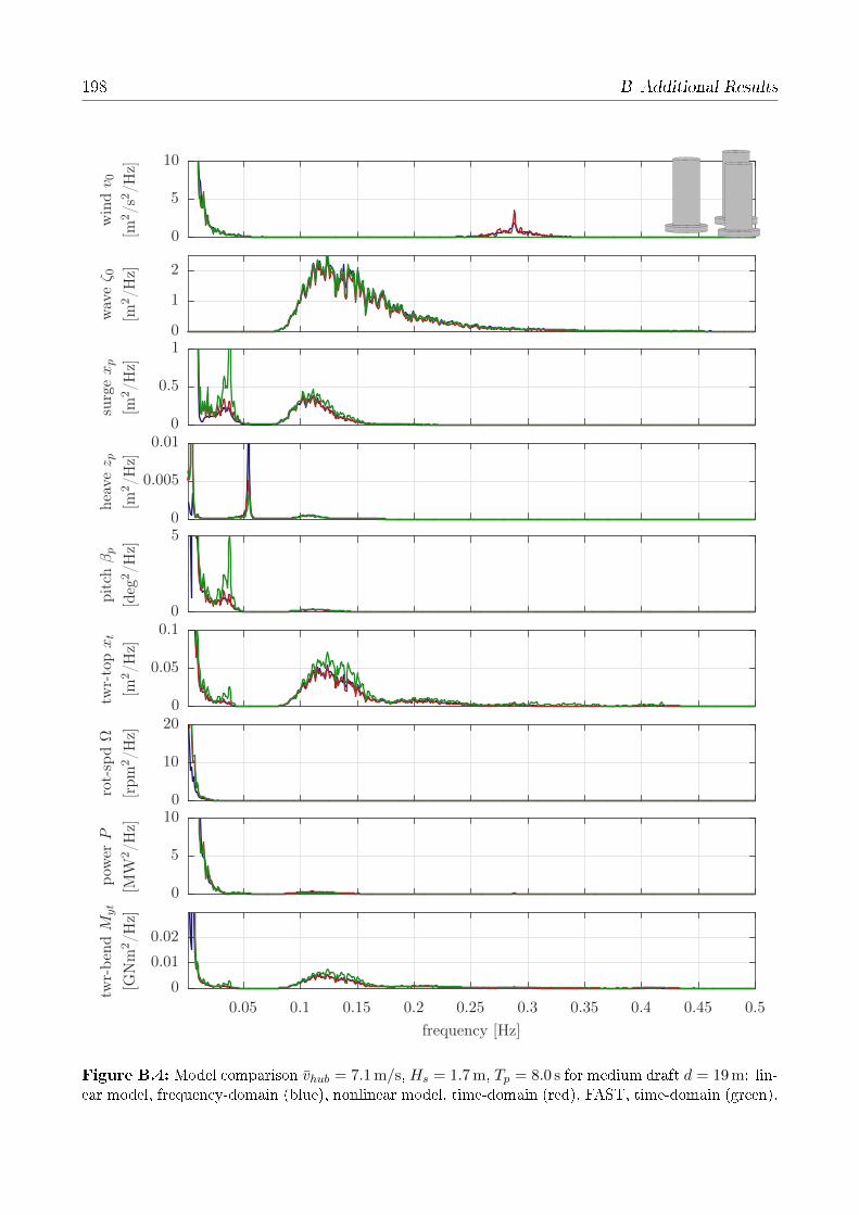
198 B Additional Results
frequency [Hz]
twr-
ben
dM
yt
[GN
m2/H
z]
pow
erP
[MW
2/H
z]
rot-
spdΩ
[rpm
2/H
z]
twr-
topxt
[m2/H
z]
pit
chβp
[deg
2/H
z]
hea
vez p
[m2/H
z]
surg
exp
[m2/H
z]
wav
eζ 0
[m2/H
z]
win
dv 0
[m2/s
2/H
z]
0.05 0.1 0.15 0.2 0.25 0.3 0.35 0.4 0.45 0.5
0
0.01
0.02
0
5
100
10
200
0.05
0.10
50
0.005
0.010
0.5
10
1
2
0
5
10
Figure B.4: Model comparison vhub = 7.1 m/s, Hs = 1.7 m, Tp = 8.0 s for medium draft d = 19 m: lin-ear model, frequency-domain (blue), nonlinear model, time-domain (red), FAST, time-domain (green).
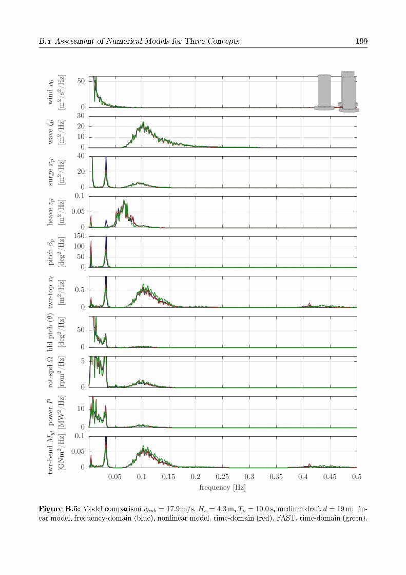
B.4 Assessment of Numerical Models for Three Concepts 199
frequency [Hz]
twr-
ben
dM
yt
[GN
m2/H
z]
pow
erP
[MW
2/H
z]
rot-
spdΩ
[rpm
2/H
z]
bld
ptc
h(θ
)
[deg
2/H
z]
twr-
topxt
[m2/H
z]
pit
chβp
[deg
2/H
z]
hea
vez p
[m2/H
z]
surg
exp
[m2/H
z]
wav
eζ 0
[m2/H
z]
win
dv 0
[m2/s
2/H
z]
0.05 0.1 0.15 0.2 0.25 0.3 0.35 0.4 0.45 0.5
0
0.05
0.10
10
0
5
0
50
0
0.5
0
50
100
1500
0.05
0.10
20
400
10
20
300
50
Figure B.5: Model comparison vhub = 17.9 m/s, Hs = 4.3 m, Tp = 10.0 s, medium draft d = 19 m: lin-ear model, frequency-domain (blue), nonlinear model, time-domain (red), FAST, time-domain (green).
200 B Additional Results
frequency [Hz]
twr-
ben
dM
yt
[GN
m2/H
z]
pow
erP
[MW
2/H
z]
rot-
spdΩ
[rpm
2/H
z]
twr-
topxt
[m2/H
z]
pit
chβp
[deg
2/H
z]
hea
vez p
[m2/H
z]
surg
exp
[m2/H
z]
wav
eζ 0
[m2/H
z]
win
dv 0
[m2/s
2/H
z]
0.05 0.1 0.15 0.2 0.25 0.3 0.35 0.4 0.45 0.5
0
0.002
0.0040
500
10
200
0.02
0.040
5
100
0.01
0.02
0
50
1
2
0
5
10
Figure B.6: Model comparison vhub = 7.1 m/s, Hs = 1.7 m, Tp = 8.0 s for low-draft d = 24 m: linearmodel, frequency-domain (blue), nonlinear model, time-domain (red), FAST, time-domain (green).
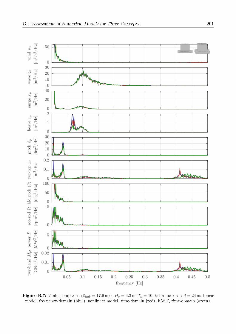
B.4 Assessment of Numerical Models for Three Concepts 201
frequency [Hz]
twr-
ben
dM
yt
[GN
m2/H
z]
pow
erP
[MW
2/H
z]
rot-
spdΩ
[rpm
2/H
z]
bld
ptc
h(θ
)
[deg
2/H
z]
twr-
topxt
[m2/H
z]
pit
chβp
[deg
2/H
z]
hea
vez p
[m2/H
z]
surg
exp
[m2/H
z]
wav
eζ 0
[m2/H
z]
win
dv 0
[m2/s
2/H
z]
0.05 0.1 0.15 0.2 0.25 0.3 0.35 0.4 0.45 0.5
0
0.01
0.020
5
0
50
50
1000
0.1
0.20
10
20
300
1
20
20
400
10
20
300
50
Figure B.7: Model comparison vhub = 17.9 m/s, Hs = 4.3 m, Tp = 10.0 s for low-draft d = 24 m: linearmodel, frequency-domain (blue), nonlinear model, time-domain (red), FAST, time-domain (green).


Bibliography
[1] James, R. and Costa Ros, M. Floating oshore wind: Market and technology review. Tech.
rep., The Carbon Trust, 2015. URL http://www.carbontrust.com/media/670664/
floating-offshore-wind-market-technology-review.pdf.
[2] Matha, D., Pérez Moran, G., Müller, K., and Lemmer, F. Comparative analysis of indus-
trial design methodologies for xed-bottom and oating wind turbines. In: Proceedings
of the ASME 35th International Conference on Ocean, Oshore and Arctic Engineering.
Busan, Korea, 2016. doi:10.1115/OMAE2016-54920.
[3] Müller, K., Lemmer, F., Borisade, F., Kretschmer, M., Gruber, J., Hagemann, L.,
Nguyen, N.-D., and Vita, L. LIFES50+ D7.4 State-of-the-art FOWT design practice
and guidelines. Tech. rep., University of Stuttgart, 2015. URL http://lifes50plus.
eu/wp-content/uploads/2015/11/GA_640741_LIFES50_D7.4.pdf.
[4] Henderson, A. Analysis tools for large oating oshore wind farms. Ph.D. thesis, Uni-
versity College London, 2000.
[5] Sclavounos, P. D., Tracy, C., and Lee, S. Floating oshore wind turbines: Responses
in a seastate, pareto optimal designs and economic assessment. In: Proceedings of the
ASME 27th International Conference on Oshore Mechanics and Arctic Engineering.
2007. doi:10.1115/OMAE2008-57056.
[6] Jonkman, J. and Matha, D. Dynamics of oshore oating wind turbinesAnalysis of three
concepts. Wind Energy, vol. 14(4):pp. 557569, 2011. doi:10.1002/we.442.
[7] Fylling, I. and Berthelsen, P. A. Windopt An optimization tool for oating support
structures for deep water wind turbines. In: Proceedings of the ASME 30th International
Conference on Ocean, Oshore and Arctic Engineering. ASME, Rotterdam, Netherlands,
2011. doi:10.1115/OMAE2011-49985.
[8] Bachynski, E. Design and dynamic analysis of tension leg platform wind turbines. Ph.D.
thesis, NTNU, 2014. ISBN 978-82-326-0096-0.
[9] Hall, M., Buckham, B., and Crawford, C. Evolving oshore wind: A genetic algorithm-
based support structure optimization framework for oating wind turbines. In: Pro-
ceedings of the OCEANS MTS/IEEE. IEEE, Bergen, Norway, 2013. doi:10.1109/
OCEANS-Bergen.2013.6608173.
[10] Larsen, T. J. and Hanson, T. D. A method to avoid negative damped low frequent tower
204 Bibliography
vibrations for a oating, pitch controlled wind turbine. Journal of Physics: Conference
Series, vol. 75, 2007. doi:10.1088/1742-6596/75/1/012073.
[11] Jonkman, J. Inuence of control on the pitch damping of a oating wind turbine. In:
Proceedings of the 46th AIAA Aerospace Sciences Meeting and Exhibit. Reno, USA, 2008.
doi:10.2514/6.2008-1306.
[12] Fischer, B. Reducing rotor speed variations of oating wind turbines by compensation
of non-minimum phase zeros. IET Renewable Power Generation, vol. 7(4):pp. 413419,
2013. doi:0.1049/iet-rpg.2012.0263.
[13] Karimirad, M. and Moan, T. A simplied method for coupled analysis of oating oshore
wind turbines. Marine Structures, vol. 27(1):pp. 4563, 2012. doi:10.1016/j.marstruc.
2012.03.003.
[14] Betti, G., Farina, M., Marzorati, A., and Scattolini, R. Modeling and control of a oating
wind turbine with spar buoy platform. In: Proceedings of the Energy Conference and Ex-
hibition (ENERGYCON), IEEE International, pp. 189194. Florence, Italy, 2012. ISBN
9781467314541.
[15] Jonkman, J. Dynamics modeling and loads analysis of an oshore oating wind tur-
bine. Ph.D. thesis, University of Colorado, 2007, URL http://www.nrel.gov/docs/
fy08osti/41958.pdf.
[16] Lupton, R. Frequency-domain modelling of oating wind turbines. Ph.D. thesis, University
of Cambridge, 2014, URL https://www.repository.cam.ac.uk/bitstream/handle/
1810/252880/thesis.pdf.
[17] Pineda, I. and Tardieu, P. Wind in power - 2016 European statistics. Tech. rep., WindEu-
rope, 2017. URL https://windeurope.org/wp-content/uploads/files/about-wind/
statistics/WindEurope-Annual-Statistics-2016.pdf.
[18] EWEA. Wind energy scenarios for 2030. Tech. rep., European Wind Energy Associ-
ation, 2015. URL http://www.ewea.org/fileadmin/files/library/publications/
reports/EWEA-Wind-energy-scenarios-2030.pdf.
[19] International Energy Agency. World energy outlook 2017. Tech. rep., 2017. URL http:
//www.iea.org/Textbase/npsum/weo2017SUM.pdf.
[20] Arapogianni, A., Genachte, A.-B., Manzanas Ochagavia, R., Pascual Vergara, J., Castell,
D., Rodriguez Tsouroukdissian, A., Korbijn, J., Bolleman, N. C. F., Huera-Huarte, F.,
Schuon, F., Ugarte, A., Sandberg, J., de Laleu, V., Maciel, J., Tunbjer, A., Roth, R.,
de la Gueriviere, P., Coulombeau, P., Jedrec, S., Philippe, C., Voutsinas, S., Weinstein,
A., Vita, L., Byklum, E., Hurley, W. L., and Grubel, H. Deep water - The next step
for oshore wind energy. Tech. rep., European Wind Energy Association, 2013. ISBN
9782930670041.
[21] Hanson, T. D., Skaare, B., Yttervik, R., Nielsen, F. G., and Havmøller, O. Comparison of
measured and simulated responses at the rst full scale oating wind turbine Hywind. In:

Bibliography 205
Proceedings of the European Wind Energy Association Annual Event. Brussels, Belgium,
2011. ISBN 9781618399915.
[22] Roddier, D., Cermelli, C., Aubault, A., and Peier, A. Summary and conclusions of the
full life-cycle of the WindFloat FOWT prototype project. In: Proceedings of the ASME
36th International Conference on Ocean, Oshore and Arctic Engineering. Trondheim,
Norway, 2017. doi:10.1115/OMAE2017-62561.
[23] Wang, C. M., Utsunomiya, T., Wee, S. C., and Choo, Y. S. Research on oating wind
turbines: A literature survey. The IES Journal Part A: Civil & Structural Engineering,
vol. 3(4):pp. 267277, 2010. doi:10.1080/19373260.2010.517395.
[24] Tande, J. O. G., Merz, K., Paulsen, U. S., and Svendsen, H. G. Floating oshore turbines.
Wiley Interdisciplinary Reviews: Energy and Environment, vol. 4(3):pp. 213228, 2015.
doi:10.1002/wene.130.
[25] Roddier, D., Cermelli, C., Weinstein, J., Byklum, E., Atcheson, M., Utsunomiya, T.,
Jorde, J., and Borgen, E. State-of-the-art. In: M. Atcheson and J. Cruz, eds., Floating
Oshore Wind Energy, pp. 271332. Springer, 2016. ISBN 978-3-319-29398-1. doi:10.
1007/978-3-319-29398-1.
[26] Matha, D. Impact of aerodynamics and mooring system on dynamic response of oating
wind turbines. Ph.D. thesis, University of Stuttgart, 2016. ISBN 978-3-8439-3113-7.
[27] Liu, Y., Li, S., Yi, Q., and Chen, D. Developments in semi-submersible oating foun-
dations supporting wind turbines: A comprehensive review. Renewable and Sustainable
Energy Reviews, vol. 60:pp. 433449, 2016. doi:10.1016/j.rser.2016.01.109.
[28] DNV. DNV-OS-J103: Design of oating wind turbine structures. 2013.
[29] Robertson, A. and Jonkman, J. Loads analysis of several oshore oating wind tur-
bine concepts. In: Proceedings of the 21st International Ocean and Polar Engineering
Conference, pp. 443450. Maui, USA, 2011. ISBN 9781880653968.
[30] Bottasso, C. L., Bortolotti, P., Croce, A., and Gualdoni, F. Integrated aero-structural
optimization of wind turbines. Multibody System Dynamics, vol. 38(4):pp. 317344, 2016.
doi:10.1007/s11044-015-9488-1.
[31] Pavese, C., Tibaldi, C., Zahle, F., and Kim, T. Aeroelastic multidisciplinary design
optimization of a swept wind turbine blade. Wind Energy, vol. 20(12):pp. 19411953,
2017. doi:10.1002/we.2131.
[32] Birk, L., Clauss, G. F., and Lee, J. Y. Practical application of global optimization
to the design of oshore structures. In: Proceedings of the ASME 23rd International
Conference on Oshore Mechanics and Arctic Engineering. Vancouver, Canada, 2004.
doi:10.1115/OMAE2004-51225.
[33] Kühn, M. Dynamics and design optimization of oshore wind energy conversion systems.
Ph.D. thesis, Delft University of Technology, 2003. ISBN 9076468079.
[34] Häfele, J. and Rolfes, R. Approaching the ideal design of jacket substructures for oshore
206 Bibliography
wind turbines with a Particle Swarm Optimization algorithm. In: Proceedings of the 26th
International Ocean and Polar Engineering Conference, pp. 156163. Rhodes, Greece,
2016. ISBN 9781880653883.
[35] Schafhirt, S., Zwick, D., and Muskulus, M. Reanalysis of Jacket support structure for
computer-aided optimization of oshore wind turbines with a Genetic Algorithm. Journal
of Ocean and Wind Energy, vol. 1(4):pp. 209216, 2014. doi:10.17736/23103604.
[36] Chew, K.-h., Tai, K., and Muskulus, M. Optimization of oshore wind turbine support
structures using analytical gradient-based method. Energy Procedia, vol. 80:pp. 100107,
2015. doi:10.1016/j.egypro.2015.11.412.
[37] Yeter, B., Garbatov, Y., and Soares, C. G. Risk-based multi-objective optimisation
of a monopile oshore wind turbine support structure. In: Proceedings of the ASME
36th International Conference on Ocean, Oshore and Arctic Engineering. Trondheim,
Norway, 2017. doi:10.1115/OMAE2017-617565.
[38] Kurz, T. Symbolic modeling and optimization of elastic multibody systems. Ph.D. thesis,
University of Stuttgart, 2013. ISBN 9783844020465.
[39] Jonkman, J. and Buhl, M. FAST user's guide. Tech. rep., National Renewable Energy
Laboratory, Boulder, USA, 2005.
[40] Sandner, F., Schlipf, D., Matha, D., and Cheng, P. W. Integrated optimization of
oating wind turbine systems. In: Proceedings of the ASME 33rd International Con-
ference on Ocean, Oshore and Arctic Engineering. San Francisco, USA, 2014. doi:
10.1115/OMAE2014-24244.
[41] DNV. DNV-OS-C103: Structural design of column stabilised units. 2012.
[42] Bak, C., Zahle, F., Bitsche, R., Kim, T., Yde, A., Henriksen, L., Natarajan, A., and
Hansen, M. Description of the DTU 10MW reference wind turbine. Tech. rep., Technical
University of Denmark, Roskilde, Denmark, 2013.
[43] NWTC. NWTC information portal (FAST v8). 2016. URL https://nwtc.nrel.gov/
FAST8.
[44] Burton, T., Sharpe, D., Jenkins, N., and Bossanyi, E. Wind Energy Handbook. John
Wiley and Sons, Oxford, 2nd edn., 2011. ISBN 978-0-470-69975-1.
[45] Dirlik, T. Application of computers in fatigue analysis. Ph.D. thesis, University of War-
wick, 1985, URL http://go.warwick.ac.uk/wrap/2949.
[46] Borgman, L. E. The spectral density for ocean wave forces. In: Proceedings of the Santa
Barbara Coastal Engineering Conference, pp. 147182. Santa Barbara, USA, 1965.
[47] Argyriadis, K. and Klose, M. Interaction of load analysis and structural design of
oshore wind turbines. In: Proceedings of the ASME 25th International Confer-
ence on Oshore Mechanics and Arctic Engineering. Hamburg, Germany, 2006. doi:
10.1115/OMAE2006-92081.
[48] Muskulus, M. Why design load calculations for oshore wind turbine support structures

Bibliography 207
cannot use load time series from moving rotors. In: Proceedings of the 25th Interna-
tional Ocean and Polar Engineering Conference, pp. 525529. Kona, USA, 2015. ISBN
9781880653890.
[49] van der Tempel, J. Design of support structures for oshore wind turbines. Ph.D. thesis,
Delft University of Technology, 2006. ISBN 9076468117.
[50] Matha, D., Cruz, J., Masciola, M., Bachynski, E. E., Atcheson, M., Goupee, A. J.,
Gueydon, S., and Robertson, A. N. Modelling of Floating Oshore Wind Technologies.
In: M. Atcheson and J. Cruz, eds., Floating Oshore Wind Energy, pp. 133240. Springer,
2016. ISBN 978-3-319-29398-1. doi:10.1007/978-3-319-29398-1.
[51] Jonkman, J. and Musial, W. Oshore Code Comparison Collaboration (OC3) for IEA
Task 23 Oshore Wind Technology and Deployment. Tech. rep., National Renewable
Energy Laboratory, Boulder, USA, 2010.
[52] Robertson, A., Jonkman, J., and Musial, W. Oshore Code Comparison Collaboration,
Continuation: Phase II results of a oating semisubmersible wind system. In: Proceedings
of the European Wind Energy Association Oshore Wind Conference and Exhibition.
Frankfurt, Germany, 2013.
[53] Robertson, A., Jonkman, J., Vorpahl, F., Popko, W., Qvist, J., Frøyd, L., Chen, X., Az-
cona, J., Uzunoglu, E., Guedes Soares, C., Luan, C., Yutong, H., Pencheng, F., Yde, A.,
Larsen, T., Nichols, J., Buils Urbano, R., Lei, L., Nygaard, T. A., Manolas, D., Heege, A.,
Ringdalen Vatne, S., Ormberg, H., Duarte, T., Godreau, C., Fabricius Hansen, H., Wedel
Nielsen, A., Riber, H., Le Cun, C., Beyer, F., Yamaguchi, A., Jin Jung, K., Shin, H., Shi,
W., Park, H., Alves, M., and Guérinel, M. Oshore Code Comparison Collaboration Con-
tinuation within IEA Wind Task 30: Phase II results regarding a oating semisubmersible
wind system. In: Proceedings of the ASME 33rd International Conference on Ocean, O-
shore and Arctic Engineering. San Francisco, USA, 2014. doi:10.1115/OMAE2014-24040.
[54] Robertson, A., Wendt, F., Jonkman, J. M., Popko, W., Dagher, H. J., Gueydon, S., Qvist,
J., Vittori, F., Azcona, J., Uzunoglu, E., Soares, C. G., Harries, R., Yde, A., Galinos, C.,
Hermans, K., de Vaal, B. J., Bozonnet, P., Bouy, L., Bayati, I., Bergua, R., Galvan, J.,
Mendikoa, I., Barrera, C., Shin, H., Oh, S., Molins, C., and Debruyne, Y. OC5 project
phase II: Validation of global loads of the DeepCwind oating semisubmersible wind
turbine. Energy Procedia, vol. 137:pp. 3857, 2017. doi:10.1016/j.egypro.2017.10.333.
[55] Cordle, A. and Jonkman, J. State of the art in oating wind turbine design tools. In:
Proceedings of the 21st International Ocean and Polar Engineering Conference. Maui,
USA, 2011. ISBN 9781880653968.
[56] Matha, D., Schlipf, M., Pereira, R., and Jonkman, J. Challenges in simulation of aero-
dynamics, hydrodynamics, and mooring-line dynamics of oating oshore wind turbines.
In: Proceedings of the 21st International Ocean and Polar Engineering Conference. Maui,
USA, 2011. ISBN 9781880653968.

208 Bibliography
[57] Bae, Y. H., Kim, M. H., Im, S. W., and Chang, I. H. Aero-elastic-control-oater-mooring
coupled dynamic analysis of oating oshore wind turbines. In: Proceedings of the 21st
International Ocean and Polar Engineering Conference, pp. 429435. Maui, USA, 2011.
ISBN 9781880653968.
[58] Lemmer, F., Müller, K., Pegalajar-Jurado, A., Borg, M., and Bredmose, H. LIFES50+
D4.1: Simple numerical models for upscaled design. Tech. rep., University of Stuttgart,
2016.
[59] Schwertassek, R. and Wallrapp, O. Dynamik exibler Mehrkörpersysteme: Methoden
der Mechanik zum rechnergestützten Entwurf und zur Analyse mechatronischer Systeme.
Grundlagen und Fortschritte der Ingenieurwissenschaften. Friedr. Vieweg und Sohn, 1999.
ISBN 978-3-322-93976-0.
[60] Hansen, M. O. L. Aerodynamics of Wind Turbines. Earthscan, 2nd edn., 2000. ISBN
978-1-84407-438-9.
[61] Hansen, M. O. L., Sørensen, J. N., Voutsinas, S., Sørensen, N., and Madsen, H. A. State of
the art in wind turbine aerodynamics and aeroelasticity. Progress in Aerospace Sciences,
vol. 42(4):pp. 285330, 2006. doi:10.1016/j.paerosci.2006.10.002.
[62] Guntur, S., Jonkman, J., Jonkman, B., Wang, Q., Sprague, M. A., Hind, M., Sievers, R.,
and Schreck, S. J. A validation and code-to-code verication of FAST for a megawatt-
scale wind turbine with aeroelastically tailored blades. Wind Energy Science, vol. 2:pp.
443468, 2017. doi:10.5194/wes-2-443-2017.
[63] Buils Urbano, R., Nichols, J., Livingstone, M., Cruz, J., Alexandre, A., and Mccowen,
D. Advancing numerical modelling of oating oshore wind turbines to enable ecient
structural design. In: Proceedings of the European Wind Energy Association Oshore
Wind Conference and Exhibition. Frankfurt, Germany, 2013.
[64] Luan, C., Gao, Z., and Moan, T. Development and verication of a time-domain ap-
proach for determining forces and moments in structural components of oaters with
an application to oating wind turbines. Marine Structures, vol. 51:pp. 87109, 2017.
doi:10.1016/j.marstruc.2016.10.002.
[65] Borg, M., Hansen, A. M., and Bredmose, H. Floating substructure exibility of large-
volume 10MW oshore wind turbine platforms in dynamic calculations. Journal of
Physics: Conference Series, vol. 753, 2016. doi:10.1088/1742-6596/753/8/082024.
[66] Borg, M., Bredmose, H., and Hansen, A. M. Elastic deformations of oaters for oshore
wind turbines: dynamic modelling and sectional load calculations. In: Proceedings of
the ASME 36th International Conference on Ocean, Oshore and Arctic Engineering.
Trondheim, Norway, 2017. doi:10.1115/OMAE2017-61466.
[67] Knudsen, T. and Bak, T. Simple model for describing and estimating wind turbine
dynamic inow. Proceedings of the American Control Conference, pp. 640646, 2013.
doi:10.1109/ACC.2013.6579909.
Bibliography 209
[68] Snel, H. and Schepers, J. Joint investigation of dynamic inow eects and implemen-
tation of an engineering method. Tech. rep., ECN, 1995. URL https://www.ecn.nl/
publications/E/1995/ECN-C--94-107.
[69] Merz, K., Muskulus, M., and Moe, G. A simple frequency-domain method for stress
analysis of stall-regulated wind turbines. Wind Energy, vol. 15:pp. 773798, 2012. doi:
10.1002/we.504.
[70] NWTC. NWTC information portal (AirfoilPrep). 2014. URL https://nwtc.nrel.gov/
AirFoilPrep.
[71] Snel, H. Review of the present status of rotor aerodynamics. Wind Energy, vol. 1:pp.
4669, 1998.
[72] Sant, T. Improving BEM-based aerodynamic models in wind turbine design codes. Ph.D.
thesis, Delft University of Technology, 2007. ISBN 9789993204831.
[73] Vaal, J. B. D., Hansen, M. O. L., and Moan, T. Eect of wind turbine surge motion on
rotor thrust. Wind Energy, vol. 17(1):pp. 105121, 2014. doi:10.1002/we.1562.
[74] Bayati, I., Belloli, M., Bernini, L., and Zasso, A. A formulation for the unsteady aero-
dynamics of oating wind turbines, with focus on the global system dynamics. In: Pro-
ceedings of the ASME 36th International Conference on Ocean, Oshore and Arctic En-
gineering. Trondheim, Norway, 2017. doi:10.1115/OMAE2017-61925.
[75] Suzuki, A. and Hansen, A. Generalized dynamic wake model for Yawdyn. In: Proceedings
of the AIAA18th Wind Energy Symposium, pp. 186191. Reno, USA, 1999. doi:10.2514/
6.1999-41.
[76] Moriarty, P. J. and Hansen, C. AeroDyn theory manual. Tech. rep., National Renewable
Energy Laboratory, Golden, USA, 2005. URL https://nwtc.nrel.gov/system/files/
AD_Theory.pdf.
[77] Sebastian, T. The aerodynamic and near wake of an oshore oating horizontal axis
wind turbine. Ph.D. thesis, University of Massachussetts, Amherst, USA, 2012, URL
https://scholarworks.umass.edu/open_access_dissertations/516/.
[78] Manolas, D. Hydro-aero-elastic analysis of oshore wind turbines. Ph.D. thesis, National
Technical University of Athens, 2015, URL https://dspace.lib.ntua.gr/dspace2/
bitstream/handle/123456789/42037/PhD_Manolas_DI_2015_Hydro-Aero-Elastic_
Analysis_of_Offshore_WTs.pdf.
[79] Lennie, M., Marten, D., Pechlivanoglou, G., Nayeri, C. N., and Paschereit, C. O. Modern
methods for investigating the stability of a pitching oating platform wind turbine. Jour-
nal of Physics: Conference Series, vol. 753, 2016. doi:10.1088/1742-6596/753/8/082012.
[80] Bekiropoulos, D., Rieÿ, R. M., Lutz, T., and Krämer, E. Simulation of unsteady aero-
dynamic eects on oating oshore wind turbines. In: Proceedings of the German Wind
Energy Conference DEWEK. Bremen, Germany, 2012.
[81] Tran, T. T. and Kim, D. H. The platform pitching motion of oating oshore wind
210 Bibliography
turbine: A preliminary unsteady aerodynamic analysis. Journal of Wind Engineering
and Industrial Aerodynamics, vol. 142:pp. 6581, 2015. doi:10.1016/j.jweia.2015.03.009.
[82] Sant, T., Bonnici, D., Farrugia, R., and Micallef, D. Measurements and modelling of the
power performance of a model oating wind turbine under controlled conditions. Wind
Energy, vol. 18:pp. 811834, 2015. doi:10.1002/we.1730.
[83] Lin, L., Vassalos, D., and Dai, S. CFD simulation of aerodynamic performance of oating
oshore wind turbine compared with BEM method. In: Proceedings of the 26th Interna-
tional Ocean and Polar Engineering Conference, pp. 568575. Kona, USA, 2016. ISBN
978-1-880653-88-3.
[84] Wu, C.-H. K. and Nguyen, V.-T. Aerodynamic simulations of oshore oating wind
turbine in platform-induced pitching motion. Wind Energy, vol. 20(5):pp. 835858, 2017.
doi:10.1002/we.2066.
[85] Matha, D., Wendt, F., Werner, M., Cheng, P. W., and Lutz, T. Aerodynamic inow
conditions on oating oshore wind turbine blades for airfoil design purposes. In: Pro-
ceedings of the 22nd International Ocean and Polar Engineering Conference, pp. 480488.
Rhodes, Greece, 2012. ISBN 9781880653944.
[86] Pedersen, M. and Fossen, T. Ecient nonlinear wind-turbine modeling for control appli-
cations. In: Proceedings of the 7th International Conference on Mathematical Modelling.
Vienna, Austria, 2012. doi:10.3182/20120215-3-AT-3016.00046.
[87] Sønderby, I. B. Low-order aeroelastic models of wind turbines for controller design. Ph.D.
thesis, Technical University of Denmark, 2013, URL http://orbit.dtu.dk/files/
74567482/thesis..PDF.
[88] Matha, D., Lemmer, F., and Muskulus, M. Hydrodynamics of Oshore Wind Turbines
(in production). In: P. Veers, ed., Wind Power Modelling: Turbines and Systems, vol. 2.
The IET, 2019.
[89] McCormick, M. E. Ocean Engineering Mechanics. Cambridge University Press, 2010.
ISBN 978-0-521-85952-3.
[90] Journée, J. and Massie, W. W. Oshore Hydromechanics. Delft University of
Technology, 1st edn., 2001. URL https://ocw.tudelft.nl/wp-content/uploads/
OffshoreHydromechanics_Journee_Massie.pdf.
[91] Newman, J. N. Marine Hydrodynamics. MIT Press, Cambridge, USA, 1977. ISBN
978-0-262-14026-3.
[92] Sarpkaya, T. Wave Forces on Oshore Structures. Cambridge University Press, 1st edn.,
2010. ISBN 978-0-521-89625-2.
[93] Cummins, W. The impulse response function and ship motion. In: Proceedings of the
Symposium on Ship Theory. Hamburg, Germany, 1962.
[94] Ogilvie, T. F. Recent progress toward the understanding and prediction of ship motions.
In: Proceedings of the Fifth Symposium on Naval Hydrodynamics. Bergen, Norway, 1964.

Bibliography 211
[95] Jonkman, J., Robertson, A., and Hayman, G. HydroDyn user's guide and theory manual.
Tech. rep., National Renewable Energy Laboratory, Boulder, USA, 2014. URL https:
//nwtc.nrel.gov/system/files/HydroDyn_Manual_0.pdf.
[96] Pegalajar-Jurado, A., Borg, M., and Bredmose, H. An ecient frequency-domain model
for quick load analysis of oating oshore wind turbines. Wind Energy Science, vol. 3:pp.
693712, 2018. doi:10.5194/wes-3-693-2018.
[97] Yu, Z. and Falnes, J. State-space modelling of a vertical cylinder in heave. Applied Ocean
Research, vol. 17(5):pp. 265275, 1995. doi:10.1016/0141-1187(96)00002-8.
[98] Yu, Z. and Falnes, J. State-space modeling of dynamic systems in ocean engineering.
Journal of Hydrodynamics, vol. 24(1):pp. 117, 1998.
[99] Pérez, T. and Fossen, T. Time- vs. frequency-domain identication of parametric ra-
diation force models for marine structures at zero speed. Modeling, Identication and
Control, vol. 29(1):pp. 119, 2008. doi:10.4173/mic.2008.1.1.
[100] Kristiansen, E., Hjulstad, Å., and Egeland, O. State-space representation of radiation
forces in time-domain vessel models. Modeling, Identication and Control, vol. 27(1):pp.
2341, 2006. doi:10.1016/j.oceaneng.2005.02.009.
[101] Pérez, T. and Fossen, T. A matlab toolbox for parametric identication of radiation-force
models of ships and oshore structures. Journal of Modeling, Identication and Control,
vol. 30(1):pp. 115, 2009. doi:10.4173/mic.2009.1.1.
[102] Duarte, T., Sarmento, A., Alves, M., and Jonkman, J. State-space realization of the
wave-radiation force within FAST. In: Proceedings of the ASME 32nd International
Conference on Ocean, Oshore and Arctic Engineering. Nantes, France, 2013. doi:10.
1115/OMAE2013-10375.
[103] Lemmer, F., Raach, S., Schlipf, D., and Cheng, P. W. Parametric wave excitation model
for oating wind turbines. Energy Procedia, vol. 94:pp. 290305, 2016. doi:10.1016/j.
egypro.2016.09.186.
[104] Sørensen, A., Sagatun, S., and Fossen, T. Design of a dynamic positioning system using
model-based control. Control Engineering Practice, vol. 4(3):pp. 359368, 1996. doi:
10.1016/0967-0661(96)00013-5.
[105] Lackner, M. and Rotea, M. Structural control of oating wind turbines. Mechatronics,
vol. 21(4):pp. 704719, 2011. doi:10.1016/j.mechatronics.2010.11.007.
[106] Schlipf, D., Sandner, F., Raach, S., Matha, D., and Cheng, P. W. Nonlinear model
predictive control of oating wind turbines. In: Proceedings of the 23rd International
Ocean and Polar Engineering Conference, pp. 440447. Anchorage, USA, 2013. doi:
10.18419/opus-3908.
[107] Lemmer, F., Raach, S., Schlipf, D., and Cheng, P. W. Prospects of linear model predictive
control on a 10MW oating wind turbine. In: Proceedings of the ASME 34th International
212 Bibliography
Conference on Ocean, Oshore and Arctic Engineering. St. John's, Canada, 2015. doi:
10.1115/OMAE2015-42267.
[108] Schlipf, D., Simley, E., Lemmer, F., Pao, L., and Cheng, P. W. Collective pitch feedfor-
ward control of oating wind turbines using Lidar. Journal of Ocean and Wind Energy,
vol. 2(4):pp. 223230, 2015. doi:10.17736/jowe.2015.arr04.
[109] Morison, J. R. The force distribution exerted by surface waves on piles. Tech. rep.,
University of California, Institute of Engineering Research, Berkeley, USA, 1953.
[110] Sarpkaya, T. and Isaacson, M. Mechanics of Wave Forces on Oshore Structures. Van
Nostrand Reinhold Co., 1981. ISBN 9780442254025.
[111] Jonkman, J. Denition of the oating system for phase IV of OC3. Tech. rep., National
Renewable Energy Laboratory, 2010.
[112] Robertson, A., Jonkman, J., Masciola, M., Song, H., Goupee, A., Coulling, A., and
Luan, C. Denition of the semisubmersible oating system for phase II of OC4. Tech.
rep., National Renewable Energy Laboratory, Boulder, USA, 2014. URL http://www.
nrel.gov/docs/fy14osti/60601.pdf.
[113] Östergaard, C. and Schellin, T. E. Comparison of experimental and theoretical wave
actions on oating and compliant oshore structures. Applied Ocean Research, vol. 9(4),
1987. doi:10.1016/0141-1187(87)90002-2.
[114] Brorsen, M. Slowly-varying 2nd order wave forces on large structures. Aalborg Uni-
versity, 2006. URL http://vbn.aau.dk/files/6771919/Slowly-varying_2._order_
Wave_Forces_on_Large_Structures.
[115] Faltinsen, O. M. Sea Loads On Ships And Oshore Structures. Cambridge University
Press, 1993. ISBN 0-521-45870-6.
[116] Gueydon, S., Duarte, T., and Jonkman, J. Comparison of second-order loads on a
semisubmersible oating wind turbine. In: Proceedings of the ASME 33rd International
Conference on Ocean, Oshore and Arctic Engineering. San Francisco, USA, 2014. doi:
10.1115/OMAE2014-23398.
[117] Duarte, T., Sarmento, A., and Jonkman, J. Eects of second-order hydrodynamic forces
on oating oshore wind turbines. In: Proceedings of the AIAA SciTech. National Harbor,
USA, 2014. doi:10.2514/6.2014-0361.
[118] Roald, L., Jonkman, J., Robertson, A., and Chokani, N. The eect of second-order
hydrodynamics on oating oshore wind turbines. Energy Procedia, vol. 35:pp. 253264,
2013. doi:10.1016/j.egypro.2013.07.178.
[119] Lupton, R. and Langley, R. S. Assessing the importance of the slow drift motion of oating
wind turbine platforms. In: Proceedings of the ASME 33rd International Conference
on Ocean, Oshore and Arctic Engineering. San Francisco, USA, 2014. doi:10.1115/
OMAE2014-23859.
[120] Gueydon, S. and Jonkman, J. Update on the comparison of second-order loads on a ten-

Bibliography 213
sion leg platform for wind turbines. In: Proceedings of the 26th International Ocean and
Polar Engineering Conference, pp. 323332. Rhodes, Greece, 2016. ISBN 9781880653883.
[121] Bachynski, E. and Moan, T. Second order wave force eects on tension leg platform wind
turbines in misaligned wind and waves. In: Proceedings of the ASME 33rd International
Conference on Ocean, Oshore and Arctic Engineering. San Francisco, USA, 2014. doi:
10.1115/OMAE2014-23131.
[122] Azcona, J. Computational and experimental modelling of mooring line dynamics for
oshore oating wind turbines. Ph.D. thesis, Universidad Politécnica de Madrid, 2016,
URL http://oa.upm.es/44708/1/JOSE_AZCONA_ARMENDARIZ_2.pdf.
[123] Azcona, J., Palacio, D., Munduate, X., González, L., and Nygaard, T. A. Impact of
mooring lines dynamics on the fatigue and ultimate loads of three oshore oating wind
turbines computed with IEC 61400-3 guideline. Wind Energy, vol. 20(5):pp. 797813,
2016. doi:10.1002/we.2064.
[124] Masciola, M., Robertson, A., Jonkman, J., Coulling, A., and Goupee, A. Assessment of
the importance of mooring dynamics on the global response of the DeepCwind oating
semisubmersible oshore wind turbine. In: Proceedings of the 23rd International Ocean
and Polar Engineering Conference. Anchorage, USA, 2013. ISBN 978-1 880653 99-9.
[125] Masciola, M. Instructional and theory guide to the mooring analysis program. Tech.
rep., National Renewable Energy Laboratory, 2014. URL http://wind.nrel.gov/
designcodes/simulators/map/MAP.pdf.
[126] Hall, M. MoorDyn user's guide. Tech. rep., University of Maine, Orono, USA, 2015. URL
https://nwtc.nrel.gov/MoorDyn.
[127] Matha, D., Fechter, U., Kühn, M., and Cheng, P. W. Non-linear multi-body mooring
system model for oating oshore wind turbines. In: Proceedings of the European Wind
Energy Association Oshore Wind Conference and Exhibition. Amsterdam, Netherlands,
2011.
[128] Azcona, J., Munduate, X., González, L., and Nygaard, T. Experimental validation of a
dynamic mooring lines code with tension and motion measurements of a submerged chain.
Ocean Engineering, vol. 129:pp. 415427, 2017. doi:10.1016/j.oceaneng.2016.10.051.
[129] Masciola, M., Jonkman, J., and Robertson, A. Extending the capabilities of the mooring
analysis program: A survey of dynamic mooring line theories for integration into FAST.
In: Proceedings of the ASME 33rd International Conference on Ocean, Oshore and
Arctic Engineering. San Francisco, USA, 2014. doi:10.1115/OMAE2014-23508.
[130] Hsu, W.-t., Thiagarajan, K. P., MacNicoll, M., and Akers, R. Prediction of extreme
tensions in mooring lines of a oating oshore wind turbine in a 100-year storm. In:
Proceedings of the ASME 34th International Conference on Ocean, Oshore and Arctic
Engineering. Saint John's, Canada, 2015. doi:10.1115/OMAE2015-42015.
[131] IEC. 61400-1 Wind turbines - Part 1: Design requirements. 2005.
214 Bibliography
[132] Sutherland, H. J. On the fatigue analysis of wind turbines. Tech. rep., Sandia National
Laboratories, Albuquerque, USA, 1999.
[133] Philippe, M., Babarit, A., and Ferrant, P. Comparison of time and frequency domain
simulations of an oshore oating wind turbine. In: Proceedings of the ASME 30th Inter-
national Conference on Ocean, Oshore and Arctic Engineering. Rotterdam, Netherlands,
2011. doi:10.1115/OMAE2011-49722.
[134] Kvittem, M. and Moan, T. Frequency versus time domain fatigue analysis of a semi-
submersible wind turbine tower. In: Proceedings of the ASME 33rd International Con-
ference on Ocean, Oshore and Arctic Engineering. San Francisco, USA, 2014. doi:
10.1115/OMAE2014-23385.
[135] Savenije, F. and Peeringa, J. Aero-elastic simulation of oshore wind turbines in the
frequency domain. Tech. rep., ECN, Petten, Netherlands, 2009. URL http://www.ecn.
nl/docs/library/report/2009/e09060.pdf.
[136] Larsen, T. J. and Hansen, A. M. How 2 HAWC2, the user's manual. Tech. rep., Technical
University of Denmark, Roskilde, Denmark, 2007. ISBN 9788755035836.
[137] IEC. 61400-3 Wind turbines - Part 3: Design requirements for oshore wind turbines.
2007.
[138] Veers, P. Three-dimensional wind simulation. Tech. rep., Sandia National Laboratories,
Albuquerque, USA, 1988. URL http://prod.sandia.gov/techlib/access-control.
cgi/1988/880152.pdf.
[139] Jonkman, B. and Kilcher, L. TurbSim user's guide. Tech. rep., National Renewable
Energy Laboratory, Boulder, USA, 2009. URL https://nwtc.nrel.gov/system/files/
TurbSim.pdf.
[140] IEC. 61400-3-2 TS Ed. 1 Wind turbines - Part 3-2: Design requirements for oating
oshore wind turbines (under preparation). 2018.
[141] DNV. DNV-OS-J101: Design of oshore wind turbine structures. 2014.
[142] Cheng, P. W. A reliability based design methodology for extreme response of oshore wind
turbines. Ph.D. thesis, Delft University of Technology, 2002. ISBN 90-79468-08-7.
[143] Krieger, A., Ramachandran, G. K. V., Vita, L., Gómez Alonso, P., Berque,
J., and Aguirre-Suso, G. LIFES50+ D7.2 Design basis. Tech. rep., DNV-
GL, 2016. URL http://lifes50plus.eu/wp-content/uploads/2015/11/D72_Design_
Basis_Retyped-v1.1.pdf.
[144] DIN. Eurocode 3: Design of steel structures - Part 1-9: Fatigue (DIN EN 1993-1-9).
2010.
[145] DNV. DNV-RP-C203: Fatigue design of oshore steel structures. 2011.
[146] Lotsberg, I. Fatigue Design of Marine Structures. Cambridge University Press, Cam-
bridge, 2016. doi:10.1017/CBO9781316343982.
[147] Halfpenny, A. A frequency domain approach for fatigue life estimation from Finite Ele-

Bibliography 215
ment Analysis. In: Proceedings of the International Conference on Damage Assessment
of Structures, pp. 401410. Dublin, Ireland, 1999. ISBN 0878498397.
[148] Naess, A. and Moan, T. Stochastic Dynamics of Marine Structures. Cambridge University
Press, 2012. doi:10.1017/CBO9781139021364.
[149] Bredmose, H., Larsen, S. E., Matha, D., Rettenmeier, A., Marino, E., and Saettran, L.
MARINET D2.4: Collation of oshore wind-wave dynamics. Tech. rep., Technical Uni-
versity of Denmark, 2012. URL http://orbit.dtu.dk/files/60086212/Collation_
of_offshore.pdf.
[150] Goupee, A. J., Koo, B. J., Kimball, R. W., Lambrakos, K. F., and Dagher, H. J. Ex-
perimental comparison of three oating wind turbine concepts. In: Proceedings of the
ASME 31st International Conference on Ocean, Oshore and Arctic Engineering. Rio de
Janeiro, Brazil, 2012. doi:10.1115/OMAE2012-83645.
[151] Robertson, A., Goupee, A., Jonkman, J., Prowell, I., Molta, P., Coulling, A., and Mas-
ciola, M. Summary of conclusions and recommendations drawn from the DeepCwind
scaled oating oshore wind system test campaign. In: Proceedings of the ASME
32nd International Conference on Ocean, Oshore and Arctic Engineering. 2013. doi:
10.1115/OMAE2013-10817.
[152] Vittori, F., Bouchotrouch, F., Lemmer, F., and Azcona, J. Hybrid scaled testing of a
5MW oating wind turbine using the SIL method compared with numerical models. In:
Proceedings of the ASME 37th International Conference on Ocean, Oshore and Arctic
Engineering. Madrid, Spain, 2018. doi:10.1115/OMAE2018-77853.
[153] Kanner, S., Koukina, E., and Yeung, R. W. Power optimization of model-scale oating
wind turbines using real-time hybrid testing with autonomous actuation and control. In:
Proceedings of the ASME 36th International Conference on Ocean, Oshore and Arctic
Engineering. Trondheim, Norway, 2017. doi:10.1115/OMAE2017-62175.
[154] Karimirad, M., Bachynski, E., Berthelsen, P. A., and Ormberg, H. Comparison
of real-time hybrid model testing of a braceless semi- submersible wind turbine and
numerical simulations. In: Proceedings of the ASME 36th International Conference
on Ocean, Oshore and Arctic Engineering. ASME, Trondheim, Norway, 2017. doi:
10.1115/OMAE2017-61121.
[155] Bayati, I., Belloli, M., Bernini, L., and Zasso, A. Wind tunnel validation of AeroDyn
within LIFES50+ project: Imposed surge and pitch tests. Journal of Physics: Conference
Series, vol. 753, 2016. doi:10.1088/1742-6596/753/9/092001.
[156] Müller, K., Sandner, F., Bredmose, H., Azcona, J., Manjock, A., and Pereira, R. Improved
tank test procedures for scaled oating oshore wind turbines. In: International Wind
Engineering Conference IWEC. Hannover, Germany, 2014. doi:10.18419/opus-8261.
[157] Matha, D., Sandner, F., Molins, C., Campos, A., and Cheng, P. W. Ecient preliminary
oating oshore wind turbine design and testing methodologies and application to a
216 Bibliography
concrete spar design. Philosophical Transactions of the Royal Society A, vol. 373(2035),
2015. doi:10.1098/rsta.2014.0350.
[158] Borisade, F., Koch, C., Lemmer, F., Cheng, P. W., and Matha, D. Validation of
INNWIND.EU scaled model tests of a semisubmersible oating wind turbine. Inter-
national Journal of Oshore and Polar Engineering, vol. 28(1):pp. 5464, 2017. doi:
10.17736/ijope.2018.fv04.
[159] Klein, L., Schulz, C., Lutz, T., and Krämer, E. Inuence of jet ow on the Aerodynamics
of a oating model wind turbine. In: Proceedings of the 26th International Ocean and
Polar Engineering Conference, pp. 403410. Rhodes, Greece, 2016. ISBN 9781880653883.
[160] Bredmose, H., Lemmer, F., Borg, M., Pegalajar-Jurado, A., Mikkelsen, R. F., Stoklund
Larsen, T., Fjelstrup, T., Yu, W., Lomholt, A. K., Boehm, L., and Azcona, J. The
TripleSpar campaign: Model tests of a 10MW oating wind turbine with waves, wind
and pitch control. Energy Procedia, vol. 137:pp. 5876, 2017. doi:10.1016/j.egypro.2017.
10.334.
[161] Yu, W., Lemmer, F., Bredmose, H., Borg, M., Pegalajar-Jurado, A., Mikkelsen, R. F.,
Stoklund Larsen, T., Fjelstrup, T., Lomholt, A., Boehm, L., Schlipf, D., and Azcona,
J. The TripleSpar Campaign: Implementation and test of a blade pitch controller on a
scaled oating wind turbine model. In: Energy Procedia, vol. 137, pp. 323338. Elsevier,
Trondheim, Norway, 2017. doi:10.1016/j.egypro.2017.10.357.
[162] Schlipf, D. Lidar-assisted control concepts for wind turbines. Ph.D. thesis, University of
Stuttgart, 2015. ISBN 978-3-8439-2518-1.
[163] Gasch, R. and Twele, J. Windkraftanlagen - Grundlagen, Entwurf, Planung und Betrieb.
B.G. Teubner, Wiesbaden, 4th edn., 2005. ISBN 978-3-519-36334-7.
[164] Skaare, B., Hanson, T. D., and Nielsen, F. G. Importance of control strategies on fatigue
life of oating wind turbines. In: Proceedings of the ASME 26th International Conference
on Oshore Mechanics and Arctic Engineering. San Diego, USA, 2007. doi:10.1115/
OMAE2007-29277.
[165] Veen, G. V. D., Couchman, Y., and Bowyer, R. Control of oating wind turbines. In:
Proceedings of the American Control Conference, pp. 31483153. Montreal, Canada, 2012.
doi:10.1109/ACC.2012.6315120.
[166] Skogestad, S. and Postlethwaite, I. Multivariable Feedback Control: Analysis and Design.
John Wiley and Sons, Chichester, 2nd edn., 2007. ISBN 978-0470011683. ISSN 1049-8923.
[167] Fleming, P., Pineda, I., Rossetti, M., Wright, A., and Arora, D. Evaluating methods
for control of an oshore oating turbine. In: Proceedings of the ASME 33rd Inter-
national Conference on Ocean, Oshore and Arctic Engineering. 2014. doi:10.1115/
OMAE2014-24107.
[168] Savenije, F. and Peeringa, J. Control development for oating wind. Journal of Physics:
Conference Series, vol. 524, 2014. doi:10.1088/1742-6596/524/1/012090.
Bibliography 217
[169] Vanni, F., Rainey, P., and Bossanyi, E. A comparison of control-based platform stabilisa-
tion strategies for oating wind turbines. In: Proceedings of the European Wind Energy
Association Oshore Wind Conference and Exhibition. Copenhagen, Denmark, 2015.
[170] Ritter, B. and Konigorski, U. Advanced multivariable control design for modern multi-
MW wind turbines. In: Proceedings of the EAWE 11th Phd Seminar on Wind Energy in
Europe. Stuttgart, Germany, 2015.
[171] Horowitz, I. M. Synthesis of Feedback Systems. Acad. Press, New York, USA,
1963. ISBN 978-1-4832-3282-9. URL http://www.sciencedirect.com/science/book/
9781483232829.
[172] Lindeberg, E., Svendsen, H. G., and Uhlen, K. Smooth transition between controllers for
oating wind turbines. Energy Procedia, vol. 24:pp. 8398, 2012. doi:10.1016/j.egypro.
2012.06.090.
[173] Ramos, R. Optimal vibration control of oating wind turbines in the presence of nonlin-
earities. In: Proceedings of the ASME 32nd International Conference on Ocean, Oshore
and Arctic Engineering. Nantes, France, 2013. doi:10.1115/OMAE2013-10242.
[174] Schuler, S., Schlipf, D., Cheng, P. W., and Allgöwer, F. `1-optimal control of large wind
turbines. IEEE Transactions on Control Systems Technology, vol. 21(4):pp. 10791089,
2013. doi:10.1109/tcst.2013.2261068.
[175] de Corcuera, A. D., Pujana-Arrese, A., Ezquerra, J. M., Segurola, E., and Landaluze, J.
H∞-based control for load mitigation in wind turbines. Energies, vol. 5(4):pp. 938967,
2012. doi:10.3390/en5040938.
[176] Si, Y. and Karimi, H. R. Gain scheduling H2/H∞ structural control of a oat-
ing wind turbine. IFAC Proceedings Volumes, vol. 47(3):pp. 67886793, 2014. doi:
10.3182/20140824-6-ZA-1003.02775.
[177] Christiansen, S. Model-based control of a ballast-stabilized oating wind turbine exposed
to wind and waves. Ph.D. thesis, Aalborg University, 2013, URL vbn.aau.dk/files/
77466696/thesis.pdf.
[178] Christiansen, S., Tabatabaeipour, S. M., Bak, T., and Knudsen, T. Wave disturbance
reduction of a oating wind turbine using a reference model-based predictive control. In:
Proceedings of the American Control Conference, pp. 22142219. Washington, USA, 2013.
doi:10.1109/ACC.2013.6580164.
[179] Lio, W. H., Rossiter, J. A., and Jones, B. L. A review on applications of model predictive
control to wind turbines. In: Proceedings of the UKACC 10th International Conference
on Control, pp. 680685. Loughborough, UK, 2014.
[180] Wright, A. Modern control design for exible wind turbines. Ph.D. thesis, University of
Colorado, 2004. ISBN 9780496444748.
[181] Stol, K. A. and Balas, M. J. Periodic disturbance accommodating control for blade
218 Bibliography
load mitigation in wind turbines. Journal of Solar Energy Engineering, vol. 125(4):pp.
379385, 2003. doi:10.1115/1.1621672.
[182] Namik, H. Individual blade pitch and disturbance accommodating control of oat-
ing oshore wind turbines. Ph.D. thesis, University of Auckland, 2012, URL http:
//hdl.handle.net/2292/11198%0A.
[183] Fleming, P., Peier, A., and Schlipf, D. Wind turbine controller to mitigate structural
loads on a oating wind turbine platform. In: Proceedings of the ASME 35th International
Conference on Ocean, Oshore and Arctic Engineering. Busan, Korea, 2016. doi:10.1115/
OMAE2016-54536.
[184] Stewart, G. Load reduction of oating wind turbines using tuned mass dampers. Master's
thesis, University of Massachusetts, 2012. URL https://scholarworks.umass.edu/
theses/781/.
[185] Jalili, K., Li, Y., and Rotea, M. Pitch and roll motion control of a oating wind
turbine with hybrid actuation. In: Proceedings of the ASME Dynamic Systems and
Control of Wind Energy Systems Conference. San Antonio, USA, 2014. doi:10.1115/
DSCC2014-6064.
[186] Luo, N., Bottasso, C., Karimi, H. R., and Zapateiro, M. Semiactive control for oating
oshore wind turbines subject to aero-hydro dynamic loads. In: Proceedings of the In-
ternational Conference on Renewable Energies and Power Quality. Las Palmas, Spain,
2011. ISBN 978-84-614-7527-8.
[187] Pérez-Collazo, C., Greaves, D., and Iglesias, G. A review of combined wave and oshore
wind energy. Renewable and Sustainable Energy Reviews, vol. 42:pp. 141153, 2015.
doi:10.1016/j.rser.2014.09.032.
[188] Pascu, V., Kanev, S., and van Wingerden, J.-W. Adaptive tower damping control for
oshore wind turbines. Wind Energy, vol. 20:pp. 765781, 2017. doi:10.1002/we.2058.
[189] Fischer, B. and Shan, M. A survey on control methods for the mitigation of tower loads.
Tech. rep., Fraunhofer-Institut für Windenergiesysteme, Kassel, Germany, 2013. URL
http://publica.fraunhofer.de/eprints/urn_nbn_de_0011-n-2721917.pdf.
[190] Fischer, T. Mitigation of aerodynamic and hydrodynamic induced loads of oshore wind
turbines. Ph.D. thesis, University of Stuttgart, 2012. ISBN 978-3844015010.
[191] Jost, E., Fischer, A., Lutz, T., and Krämer, E. An investigation of unsteady 3D eects
on trailing edge aps. Wind Energy Science, vol. 2:pp. 241256, 2017. doi:10.5194/
wes-2-241-201.
[192] Bossanyi, E. A. Individual blade pitch control for load reduction. Wind Energy,
vol. 6(2):pp. 119128, 2003. doi:10.1002/we.76.
[193] Yang, F., Song, Q.-w., Wang, L., Zuo, S., and Li, S.-s. Wind and wave disturbances
compensation to oating oshore wind turbine using improved individual pitch control
Bibliography 219
based on fuzzy control strategy. Abstract and Applied Analysis, 2014. doi:10.1155/2014/
968384.
[194] Lackner, M. Controlling platform motions and reducing blade loads for oating wind
turbines. Wind Engineering, vol. 33(6):pp. 541553, 2009. doi:10.1260/0309-524X.33.6.
541.
[195] Navalkar, S., van Wingerden, J.-W., Fleming, P., and van Kuik, G. A. M. Integrating
robust Lidar-based feedforward with feedback control to enhance speed regulation of
oating wind turbines. In: Proceedings of the American Control Conference. Chicago,
USA, 2015. doi:10.1109/ACC.2015.7171804.
[196] Raach, S., Schlipf, D., Sandner, F., Matha, D., and Cheng, P. W. Nonlinear model
predictive control of oating wind turbines with individual pitch control. In: Proceedings
of the American Control Conference. Portland, Oregon, USA, 2014.
[197] Skaare, B., Hanson, T. D., Nielsen, F. G., Yttervik, R., Hansen, A. M., Thomsen, K.,
and Larsen, T. J. Integrated dynamic analysis of oating oshore wind turbines. In:
Proceedings of the European Wind Energy Conference. Milan, Italy, 2007.
[198] Henriksen, L. C., Hansen, M. O. L., and Poulsen, N. K. Beyond the cp-curve in model-
based control of wind turbines. In: Proceedings of the European Wind Energy Association
Annual Event. Copenhagen, Denmark, 2012.
[199] Leithead, W., Dominguez, S., and Spruce, C. Analysis of tower/blade interaction in the
cancellation of the tower fore-aft mode via control. In: Proceedings of the European Wind
Energy Conference. London, UK, 2004.
[200] Sandner, F., Yu, W., Matha, D., Azcona, J., Munduate, X., Grela, E.,
Voutsinas, S., and Natarajan, A. INNWIND.EU D4.33: Innovative con-
cepts for oating structures. Tech. rep., University of Stuttgart, 2014. URL
http://www.innwind.eu/-/media/Sites/innwind/Publications/Deliverables/
DeliverableD4-33_Innovative-Concepts-for-Floating-Structures_INNWIND-EU.
[201] Skaare, B. Development of the Hywind concept. In: Proceedings of the ASME 36th In-
ternational Conference on Ocean, Oshore and Arctic Engineering. Trondheim, Norway,
2017. doi:10.1115/OMAE2017-62710.
[202] Molins, C., Campos, A., Sandner, F., and Matha, D. Monolithic concrete o-shore oating
structure for wind turbines. In: Proceedings of the European Wind Energy Association
Annual Event. Barcelona, Spain, 2014.
[203] Lemmer, F., Amann, F., Raach, S., and Schlipf, D. Denition of the SWE-
TripleSpar platform for the DTU10MW reference turbine. 2016. URL http://www.
ifb.uni-stuttgart.de/windenergie/downloads.
[204] Lemmer, F., Yu, W., Schlipf, D., and Cheng, P. W. Multibody modeling for concept-level
oating oshore wind turbine design (submitted and under review). Multibody System
Dynamics, 2019.

220 Bibliography
[205] Lemmer, F., Schlipf, D., and Cheng, P. W. Control design methods for oating wind
turbines for optimal disturbance rejection. Journal of Physics: Conference Series, vol.
753, 2016. doi:10.18419/opus-8906.
[206] Schiehlen, W. and Eberhard, P. Applied Dynamics. Springer International Publishing,
1st edn., 2014. doi:10.1007/978-3-319-07335-4.
[207] Seifried, R. Dynamics of Underactuated Multibody Systems: Modeling, Control and Op-
timal Design. Springer International Publishing, 2014. doi:10.1007/978-3-319-01228-5.
[208] Kane, T. R. and Levinson D. A. Dynamics: Theory and Applications. McGraw-Hill Inc.,
New York, 1985. ISBN 0-07-037846-0.
[209] Woernle, C. Mehrkörpersysteme: Eine Einführung in die Kinematik und Dynamik
von Systemen starrer Körper. Springer Vieweg, 2nd edn., 2011. doi:10.1007/
978-3-662-46687-2.
[210] Bauchau, O. Flexible Multibody Dynamics, vol. 176 of Solid Mechanics and its Applica-
tions. Springer Netherlands, Dordrecht, 1st edn., 2011. ISBN 978-94-007-0334-6.
[211] Dresig, H. and Holzweiÿig, F. Maschinendynamik. Springer, Berlin, Heidelberg, 11th
edn., 2012. doi:10.1007/978-3-642-29571-3.
[212] Nygaard, T. A., De Vaal, J., Pierella, F., Oggiano, L., and Stenbro, R. Development,
verication and validation of 3DFloat; Aero-servo-hydro-elastic computations of oshore
structures. Energy Procedia, vol. 94:pp. 425433, 2016. doi:10.1016/j.egypro.2016.09.210.
[213] Wang, Q., Sprague, M. A., Jonkman, J., Johnson, N., and Jonkman, B. BeamDyn: A
high-delity wind turbine blade solver in the FAST modular framework. Wind Energy,
vol. 20:pp. 14391462, 2017. doi:10.1002/we.2101.
[214] Shabana, A. A. Dynamics of Multibody Systems. Cambridge University Press, 3rd edn.,
2005. ISBN 0-521-85011-8.
[215] Holzwarth, P. Modellordnungsreduktion für substrukturierte mechanische Systeme. Ph.D.
thesis, University of Stuttgart, 2017. ISBN 978-3-8440-5234-3.
[216] Holm-Jørgensen, K. and Nielsen, S. R. System reduction in multibody dynamics of
wind turbines. Multibody System Dynamics, vol. 21(2):pp. 147165, 2009. doi:10.1007/
s11044-008-9132-4.
[217] Bir, G. S. User's guide to BModes. Tech. rep., NREL, 2007. URL https://nwtc.nrel.
gov/system/files/BModes.pdf.
[218] Fossen, T. Handbook of Marine Craft Hydrodynamics and Motion Control. John Wiley
and Sons, 1st edn., 2011. doi:10.1002/9781119994138.
[219] Wallrapp, O. Standardization of exible body modeling in multibody system codes, part
I: Denition of standard input data. Mechanics of Structures and Machines, vol. 22(3):pp.
283304, 1994. doi:10.1080/08905459408905214.
[220] Taghipour, R., Pérez, T., and Moan, T. Hybrid frequency-time domain models for dy-
Bibliography 221
namic response analysis of marine structures. Ocean Engineering, vol. 35(7):pp. 685705,
2008. doi:10.1016/j.oceaneng.2007.11.002.
[221] Falnes, J. On non-causal impulse response functions related to propagating water
waves. Applied Ocean Research, vol. 17(6):pp. 379389, 1995. doi:10.1016/S0141-1187(96)
00007-7.
[222] Ljung, L. System Identication - Theory for the User. Prentice-Hall, Upper Saddle River,
USA, 2nd edn., 2009. ISBN 0-13-656695-2.
[223] NWTC. NWTC Information Portal (OpenFAST). URL https://nwtc.nrel.gov/
OpenFAST.
[224] Jonkman, J., Wright, A. D., Hayman, G. J., and Robertson, A. N. Full-system lin-
earization for oating oshore wind turbines in OpenFAST (pre-print). In: Proceedings
of the ASME 2018 1st International Oshore Wind Technical Conference. ASME, San
Francisco, USA, 2018.
[225] Fossen, T. Nonlinear unied state-space model for ship maneuvering and control in a
seaway. International Journal of Bifurcation and Chaos, vol. 15(9):pp. 27172746, 2005.
doi:10.1142/S0218127405013691.
[226] Lemmer, F., Yu, W., and Cheng, P. W. Iterative frequency-domain response of oat-
ing wind turbines with parametric drag. Journal of Marine Science and Engineering,
vol. 6(4), 2018. doi:10.3390/jmse6040118.
[227] Sumer, B. M. and Fredsøe, J. Hydrodynamics Around Cylindrical Structures. World
Scientic, Singapore, 1st edn., 1997. ISBN 978-981-270-039-1.
[228] Wolfram, J. On alternative approaches to linearization and Morison's equation for wave
forces. Proceedings of the Royal Society A: Mathematical, Physical and Engineering Sci-
ences, vol. 455(1988):pp. 29572974, 1999. doi:10.1098/rspa.1999.0434.
[229] Langley, R. On the time domain simulation of second order wave forces and in-
duced responses. Applied Ocean Research, vol. 8(3):pp. 134143, 1986. doi:10.1016/
S0141-1187(86)80012-8.
[230] Tao, L. and Dray, D. Hydrodynamic performance of solid and porous heave plates. Ocean
Engineering, vol. 35(10):pp. 10061014, 2008. doi:10.1016/j.oceaneng.2008.03.003.
[231] Newman, J. N. Second-order, slowly-varying forces on vessels in irregular waves. In:
Proceedings of International Symposium on Dynamics of Marine Vehicles and Structures
in Waves. London, UK, 1974.
[232] Standing, R., Brendling, W., and Wilson, D. Recent developments in the analysis of
wave drift forces, low-frequency damping and response. In: Proceedings of the Oshore
Technology Conference. Houston, USA, 1987. doi:10.4043/5456-MS.
[233] Azcona, J., Vittori, F., Schmidt Paulsen, U., Savenije, F., Kapogiannis, G., Karvelas,
X., Manolas, D., Voutsinas, S., Amann, F., Faerron-Guzmán, R., and Lemmer, F. IN-
222 Bibliography
NWIND.EU D4.37: Design solutions for 10MW oating oshore wind turbines. Tech.
rep., CENER, 2017.
[234] Matha, D., Sandner, F., and Schlipf, D. Ecient critical design load case identication
for oating oshore wind turbines with a reduced nonlinear model. Journal of Physics:
Conference Series, vol. 555, 2014. doi:10.1088/1742-6596/555/1/012069.
[235] Sandner, F., Schlipf, D., Matha, D., Seifried, R., and Cheng, P. W. Reduced nonlinear
model of a spar-mounted oating wind turbine. In: Proceedings of the German Wind
Energy Conference DEWEK. Bremen, Germany, 2012. doi:10.18419/opus-4528.
[236] Olondriz, J., Yu, W., Jugo, J., Lemmer, F., Elorza, I., Alonso-Quesada, S., and Pujana-
Arrese, A. Using multiple delity numerical models for oating oshore wind turbine
advanced control design. Energies, vol. 11(9), 2018. doi:10.3390/en11092484.
[237] Lemmer, F., Müller, K., Yu, W., Schlipf, D., and Cheng, P. W. Optimization of oating
oshore wind turbine platforms with a self-tuning controller. In: Proceedings of the ASME
36th International Conference on Ocean, Oshore and Arctic Engineering. Trondheim,
Norway, 2017. doi:10.1115/OMAE2017-62038.
[238] Yu, W., Lemmer, F., Schlipf, D., Cheng, P. W., Visser, B., Links, H., Gupta, N., Danke-
mann, S., Couñago, B., and Serna, J. Evaluation of control methods for oating oshore
wind turbines. Journal of Physics: Conference Series, vol. 1104:p. 012033, 2018. doi:
10.1088/1742-6596/1104/1/012033.
[239] Luhmann, B., Seyedin, H., and Cheng, P. W. Numerical investigation of the load re-
duction potential of a exible hub connection on two-bladed wind turbines. Journal of
Physics: Conference Series, vol. 753, 2015. doi:10.1088/1742-6596/753/8/082013.
[240] Lemmer, F., Yu, W., Cheng, P. W., Pegalajar-Jurado, A., Borg, M., Mikkelsen, R., and
Bredmose, H. The TripleSpar campaign: Validation of a reduced-order simulation model
for oating wind turbines. In: Proceedings of the ASME 37th International Conference
on Ocean, Oshore and Arctic Engineering. ASME, Madrid, Spain, 2018. doi:10.1115/
OMAE2018-78119.
[241] Yu, W. Modeling, control design and testing of a scaled oating oshore wind turbine.
Master's thesis, University of Stuttgart, 2016.
[242] Fjelstrup, T. and Larsen, T. S. Experimental study of a triple spar oating wind turbine
in wind and wave forcing. Master's thesis, Technical University of Denmark, 2016.
[243] Chujo, T., Minami, Y., Nimura, T., and Ishida, S. Experimental study for spar type
oating oshore wind turbine with blade-pitch control. In: Proceedings of the ASME 32nd
International Conference on Ocean, Oshore and Arctic Engineering. Nantes, France,
2013. doi:10.1115/OMAE2013-10649.
[244] Goupee, A. J., Kimball, R. W., and Dagher, H. J. Experimental observations of active
blade pitch and generator control inuence on oating wind turbine response. Renewable
Energy, vol. 104:pp. 919, 2017. doi:10.1016/j.renene.2016.11.062.
Bibliography 223
[245] Savenije, F. Model testing of a oating wind turbine including control. In: EERA
Deepwind. Trondheim, Norway, 2017.
[246] Hara, N., Tsujimoto, S., Nihei, Y., Iijima, K., and Konishi, K. Experimental validation of
model-based blade pitch controller design for oating wind turbines: System identication
approach. Wind Energy, vol. 20(7):pp. 11871206, 2017. doi:10.1002/we.2089.
[247] Pegalajar-Jurado, A., Hansen, A. M., Laugesen, R., Mikkelsen, R. F., Borg, M., Kim, T.,
Heilskov, N. F., and Bredmose, H. Experimental and numerical study of a 10MW TLP
wind turbine in waves and wind. Journal of Physics: Conference Series, vol. 753, 2016.
doi:10.1088/1742-6596/753/9/092007.
[248] Berthelsen, P. A., Bachynski, E., Karimirad, M., and Thys, M. Real-time hybrid model
tests of a braceless semi-submersible wind turbine. part III: Calibration of a numerical
model. In: Proceedings of the ASME 35th International Conference on Ocean, Oshore
and Arctic Engineering. ASME, Busan, Korea, 2016. doi:10.1115/OMAE2016-54640.
[249] Lemmer, F., Schlipf, D., and Cheng, P. W. Robust gain scheduling control of oating
oshore wind turbines (submitted and under review). Wind Energy, 2019.
[250] Åström, K. J. and Murray, R. M. Feedback Systems. Princeton University Press, 2nd
edn., 2016. ISBN 9781400828739.
[251] Lemmer, F., Müller, K., Yu, W., Faerron-Guzmán, R., and Kretschmer, M. LIFES50+
D4.3: Optimization framework and methodology for optimized oater design. Tech. rep.,
University of Stuttgart, 2016. URL http://lifes50plus.eu/wp-content/uploads/
2015/11/GA_640741_LIFES50_D4.3-web.pdf.
[252] Lemmer, F., Müller, K., Yu, W., and Cheng, P. W. Semi-submersible wind turbine hull
shape design for a favorable system response behavior (submitted, revised version under
preparation). Marine Structures, 2019.
[253] Hanna, S. Y. Wave cancellation eects and extreme wave dynamics. In: Proceedings of
the Oshore Technology Conference. Houston, USA, 1986.
[254] Manolas, D., Karvelas, C., Kapogiannis, I., Riziotis, V., Spiliopoulos, K., and Voutsinas,
S. A comprehensive method for the structural design and verication of the INNWIND
10MW tri-spar oater. Journal of Physics: Conference Series, vol. 1104:p. 012025, 2018.
doi:10.1088/1742-6596/1104/1/012025.
[255] Benveniste, G., Lerch, M., de Prada, M., Kretschmer, M., Berque, J., López, A., and
Pérez-Morán, G. LIFES50+ D2.2 LCOE tool description, technical and environmen-
tal impact evaluation procedure. Tech. rep., Catalonia Institute for Energy Research,
Barcelona, Spain, 2015. URL http://lifes50plus.eu/wp-content/uploads/2016/10/
GA_640741_D2.2-internal.pdf.
[256] DNV-GL. DNVGL-RP-C205: Environmental conditions and environmental loads. Tech.
rep., DNV-GL, 2017. URL https://rules.dnvgl.com/docs/pdf/DNV/codes/docs/
2014-04/RP-C205.pdf.
224 Bibliography
[257] Yu, W., Müller, K., Lemmer, F., Schlipf, D., Bredmose, H., Borg, M., Landbø, T., and
Andersen, H. LIFES50+ D4.2 Public denition of the two LIFES50+ 10MW oater
concepts. Tech. rep., University of Stuttgart, 2017.
[258] Pegalajar-Jurado, A., Bredmose, H., Borg, M., Straume, J., Landbø, T., Andersen, H.,
Yu, W., Müller, K., and Lemmer, F. State-of-the-art model for the LIFES50+ OO-Star
Wind Floater Semi 10MW oating wind turbine. Journal of Physics: Conference Series,
vol. 1104:p. 012024, 2018. doi:10.1088/1742-6596/1104/1/012024.
[259] Skogestad, S. and Wol, E. Controllability measures for disturbance rejection. Journal
of Modeling, Identication and Control, vol. 17(3):pp. 167182, 1996. doi:10.4173/mic.
1996.3.1.

Curriculum Vitae
Frank Lemmer (né Sandner) was born on September, 29, 1985 in
Ostldern-Ruit, Germany.
He received his Diplomingenieur's degree (Dipl.-Ing.) in mechanical engineering in 2012 from
the University of Stuttgart with specializations in dynamic systems and hydraulic machinery.
Through a scholarship oered by the German-American Fulbright Commission he was able to
spend two semesters (20092010) at the University of Michigan, Ann Arbor, USA, studying
electromechanical systems and ocean energy converters. In December 2010 he completed an
internship at Alstom S.A. in the eld of gas turbine structural analysis. An additional, voluntary
internship in 2011 with the German development cooperation GIZ in Bénin gave him valuable
insight into the eld of agricultural transformation and engineering works in West Africa. After
his return to Stuttgart he completed his studies and graduated with the thesis entitled Reduced
Model Design of a Floating Wind Turbine.
He has worked as researcher at the University of Stuttgart at Stuttgart Wind Energy (SWE)
since then. His project work focused on integrated conceptual design of oating wind turbine
systems with a focus on coupled dynamic modeling and controls. The involvement in the EU-
funded projects AFOSP, INNWIND.EU and LIFES50+ helped him to gain valuable experience
in the eld of oating oshore wind.
He has chaired dierent sessions at the ASME International Conference on Ocean, Oshore
and Arctic Engineering and was invited as a lecturer to the International Summer School
on Stochastic Dynamics of Wind Turbines and Wave Energy Absorbers in Aalborg, Denmark.
During the time as researcher at SWE, he has supervised more than 15 Bachelor's and Master's
theses. He has authored and co-authored more than 20 papers in proceedings of international
conferences and one book section, which is currently under production. Four papers on the
present work have been submitted to international scientic journals, of which one is already
published at the time of publication of this thesis.
Recommended