First report of a novel multiplexer pumping system coupled to a waterquality probe to collect high temporal frequency in situ waterchemistry measurements at multiple sites
Francois Birgand,*1 Kyle Aveni-Deforge,1 Brad Smith,2 Bryan Maxwell,1 Marc Horstman,3
Alexandra B. Gerling,4 Cayelan C. Carey4
1Department of Biological and Agricultural Engineering, North Carolina State University, Raleigh, North Carolina2Sungate Design Group, Raleigh, North Carolina3WK Dickson & Co., Inc., Raleigh, North Carolina4Department of Biological Sciences, Virginia Tech, Blacksburg, Virginia
Abstract
The increasing availability and use of high-frequency water quality sensors has enabled unprecedented
observations of temporal variability in water chemistry in aquatic ecosystems. However, we remain limited
by the prohibitive costs of these probes to explore spatial variability in natural systems. To overcome this
challenge, we have developed a novel auto-sampler system that sequentially pumps water from up to 12 dif-
ferent sites located within a 12 m radius to a single water quality probe. This system is able to generate high
temporal frequency in situ water chemistry data from multiple replicated units during experiments as well as
multiple sites and depths within natural aquatic ecosystems. Thus, with one water quality probe, we are able
to observe rapid changes in water chemistry concentrations over time and space. Here, we describe the cou-
pled multiplexer-probe system and its performance in two case studies: a mesocosm experiment examining
the effects of water current velocity on nitrogen dynamics in constructed wetland sediment cores and a
whole-ecosystem manipulation of redox conditions in a reservoir. In both lotic and lentic case studies, we
observed minute-scale changes in nutrient concentrations, which provide new insight on the variability of
biogeochemical processes. Moreover, in the reservoir, we were able to measure rapid changes in metal con-
centrations, in addition to those of nutrients, in response to changes in redox. Consequently, we believe that
this coupled system holds great promise for measuring biogeochemical fluxes in a diverse suite of aquatic
ecosystems and experiments.
Until recently, most water quality data from aquatic eco-
systems have been collected on a coarse temporal frequency,
e.g., monthly, biweekly, weekly, and only rarely on daily or
more frequent time scales. It is now well established that
water chemistry can vary dramatically within minutes to
hours in streams and rivers due to changes in flow (e.g.,
Chapin et al. 2004; Pellerin et al. 2009, 2011; Birgand et al.
2010), and even in lakes and reservoirs with longer residence
times (e.g., Watras et al. 2015, 2016). There is emerging evi-
dence that, even in the absence of changes in flow, there
can be sizable and rapid changes in nutrient and metal con-
centrations likely associated with several biogeochemical
processes (e.g., Nimick et al. 2011; Cohen et al. 2012, 2013;
Hensley et al. 2015). However, the lack of established tools
for measuring rapid changes in water chemistry in situ repre-
sents a major challenge that has historically hindered the
study of biogeochemistry at the minute scale in the aquatic
environment.
New portable wet chemistry labs and optical sensors have
enabled the opportunity of measuring water chemistry con-
centrations multiple times per hour at single monitoring sta-
tions, providing invaluable information on the temporal
scale at which biogeochemical dynamics occur (e.g., Cohen
et al. 2012, 2013; Etheridge et al. 2014). Given the consider-
able advances in our understanding of aquatic biogeochemis-
try gained by the deployment of high-frequency sensors at
individual sites, it becomes obvious that measuring high-
frequency temporal variability in water chemistry at multiple
sites would likely reveal new insight on spatial heterogeneity
and processes driving variability in water chemistry coupled
in space and time. However, the current cost of in situ water
quality probes remains a major obstacle to the concurrent
This article was published online on 29 July 2016. The authors identifiedthat a co-author was missing. The correction was made and published
on 21 September 2016.*Correspondence: [email protected]
767
LIMNOLOGYand
OCEANOGRAPHY: METHODS Limnol. Oceanogr.: Methods 14, 2016, 767–783VC 2016 Association for the Sciences of Limnology and Oceanography
doi: 10.1002/lom3.10122

acquisition of both high-resolution temporal and spatial
data.
In this article, we propose an affordable system that offers
a compromise maximizing both spatial and temporal resolu-
tion for measuring water chemistry on the minute scale. We
have coupled an UV-vis (Ultraviolet-visible) spectrophotome-
ter probe with a multiplexer pumping system (MPS), which
can sequentially pump water from up to 12 sources or points
in space located within a limited distance of the probe, such
that the temporal resolution at each of the 12 sites could be
hourly at a minimum. This article describes the coupled
MPS-water quality probe system, reports an evaluation of its
performance, and presents two applications for wetland mes-
ocosms and a reservoir.
Materials and procedures
Coupled MPS-water quality probe system description
Overview
To remain affordable, the system uses a single high-
frequency automatic water quality probe as the central ana-
lytical instrument to which water from different sampling
sites (hereafter, point sources) are pumped via a MPS (Fig. 1).
Our design criteria when constructing the MPS system were:
(1) to have the capacity of obtaining hourly or sub-hourly
samples for measuring multiple point sources, (2) to be able
to pump water from the point sources to the probe to
overcome at least 3 m of head difference, (3) to be able to
run on 12 volts (V) direct current (DC) power for field
deployment, and (4) that the coupled MPS-water quality
probe system functioned entirely automatically. An accept-
able compromise for these criteria was to design an MPS sys-
tem that enabled sampling from up to 12 point source sites
located within 12 m of the central probe. We note that this
distance could be extended, possibly even doubled, with the
appropriate tubing at the cost of reduced temporal resolu-
tion on each point source.
As the in situ field spectrophotometer can only collect
one measurement at a time on fixed time intervals, we
designed and built an MPS to sequentially pump and purge
water from each point source to the probe, in synchrony
with the probe measurements, and cycle through the
sequence of measurements to obtain at least hourly time res-
olution of data collection at each source. To maintain the
water quality probe’s capability of measuring small sus-
pended particle concentrations, we chose 3.18 mm internal
diameter flexible tubing as a sampling conduit of water from
the point source to the probe, fitted with 1.5 mm mesh
screens at the source (although only dissolved constituent
applications are shown in this article). Consequently, the
coupled MPS-water quality probe system is well suited for
applications where the source sampling volume is not limit-
ed and does not affect the process or system studied.
Fig. 1. (a) Schematic of the water quality probe fitted with the Multiplexer Pumping System (MPS) for the automatic and sequential measurement of
water quality for up to 12 individual observation sources; (b) photograph of the MPS and probe system during deployment in the field configured tosample five distinct point sources (photo credit to C.C. Carey); the S::CAN Spectro::lyserTM water quality probe is fitted with the manufacturer’s
40 mL cuvette transformed into a flow-through cell.
Birgand et al. High-resolution water chemistry in time and space
768

Water quality probe
The high-frequency automatic water quality probe used
in our two applications was the field spectrophotometer
Spectro::lyserTM (S::CANTM, Vienna, Austria). The probe has
a 35 mm optical pathlength to measure nitrate, dissolved
organic carbon (DOC), total organic carbon (TOC) concen-
trations, and turbidity from light absorbance spectra
obtained from 216 wavelengths at 2.5 nm intervals between
220 nm and 737.5 nm. Several recent studies have demon-
strated that the capabilities of these probes may in fact be
greater than advertised as it is possible to create statistically
significant correlations between additional light-absorbing
and non-absorbing elements and contaminants in water
(Rieger et al. 2006; Torres and Bertrand-Krajewski 2008;
Etheridge et al. 2014). We report in this article the use of
the probe for nitrate and additional parameters listed
below.
Multiplexer pumping system overview
The seven components of the MPS include 12 in-line
three-way solenoid valves and manifold, a peristaltic pump
fitted with an H-bridge for current inversion, 3.18 mm poly-
propylene tubing, a flow-through cuvette, a storage tubing
spool, and a programmable Arduino (Arduino, www.arduino.
cc) micro-controller (Fig. 1). We designed the pumping sys-
tem to accommodate three usage modes so that after the
sensor reading, water could be (1) pumped entirely back to
its source (“purge back to source”), (2) purged to a designat-
ed sampling port (“purge back to sampling port”), or (3)
could be discarded (“pump/purge to discard”). The first two
cases require bidirectional pumping capabilities and the pres-
ence of a storage tubing spool described herein, while in the
third case, unidirectional pumping could theoretically
suffice.
Solenoid valve manifold
The manifold is made of 12 in-line, three-way, 3.4 watt
(W) solenoid valves (Model WTB-3R(K)-M6(14U)F—Takasago
Fluidic Systems, Nagoya, Japan). In Fig. 1a, eleven valves are
dedicated to different point sources and the twelfth one to a
standard solution. All valves (2 mm inside diameter) are in-
line with each other. Each valve’s output feeds directly into
the preceding valve’s input except for the ending valve,
which has its output feeding directly into the pump (Fig. 1).
The inherent design of the in-line manifold implies that
cross-contamination for water that is pumped through the
valve furthest from the pump is potentially higher than for
water pumped through the valve closest to the pump. We
have devised several solutions to address this problem (see
below). Valves are opened, or actuated, upon a 12 V DC sig-
nal from the controller. An important artifact of solenoid
valves is that a voltage spike of >100 V can occur when the
valves are closing due to the collapse of the magnetic field
existing in the solenoid. To protect the microcontroller from
this voltage surge, we installed an IRF 630 Field Effect Tran-
sistor (FET) and a 1N4007 Diode for each valve.
Peristaltic pump and H-bridge
We chose a peristaltic pump (M500, Clark SolutionsTM,
Hudson, Massachusetts, U.S.A.) that runs on 12 V DC and
consumes 12 W when pumping at maximum flow rate of
390 mL min21. A sample can be pumped from 12 m distance
from the MPS and can overcome a 3 m head difference with-
in 40 s.
Although unidirectional pumping was theoretically possi-
ble for the “pump/purge to discard” mode, we could not
assume plug flow in the cuvettes used. To minimize cross
contamination and mixing among consecutive samples, we
chose to always reverse pumping direction for all three
pumping usage modes, i.e., purge the flow-through cuvettes
and storage spiral tubing (described below) with air. Bidirec-
tional pumping was obtained using a custom-made H-Bridge
electronic circuit. We built a circuit that inverts polarity at
the motor electrodes to trigger either pumping or purging
upon a 12 V signal from the controller. The current to power
the motor goes directly through the H-bridge and avoids the
Arduino, thereby protecting the controller.
Flow-through cuvette
The Spectro::lyserTM probe measures the absorbance of
light through the water placed between the emitting and
receiving optical lenses. Total absorbance of the sample
depends on the optical pathlength and the cumulative
absorbance of all light-absorbing elements in water.
Although the instrument is designed to be immersed in situ,
the application described here keeps the instrument out of
the water and uses flow-through cuvettes or cells into which
sample water is pumped. Ideally, the optical pathlength
should be as long as possible to increase resolution on each
measurement and increase the signal to noise ratio, but
short enough to prevent too much light from being absorbed
to make reliable measurements, which can occur, e.g., in
very turbid waters.
To optimize measurements for variable absorbance values
and ranges, we used two sizes of cuvettes for the two case
studies. In the wetland mesocosm case study, we used a
quartz flow-through cuvette (Starna Cells, Inc. model 46-Q-
10; Hainault, UK) with an optical pathlength of 10 mm and
volume of 4 mL of water. In this configuration, water never
touches the instrument optics. In the reservoir case study,
the manufacturer’s 40 mL calibration cell for the S::CAN
probe was transformed into a flow-through cell by adding
inlet and outlet ports to use the default 35 mm pathlength
of the Spectro::lyserTM probe for water with low absorbance
values.
Sensor quality assurance/quality control (QA/QC)
To minimize sample cross-contamination, the flow-
through cuvette volume is pumped through the cuvette sev-
eral times to ensure thorough rinsing of the manifold pump
Birgand et al. High-resolution water chemistry in time and space
769
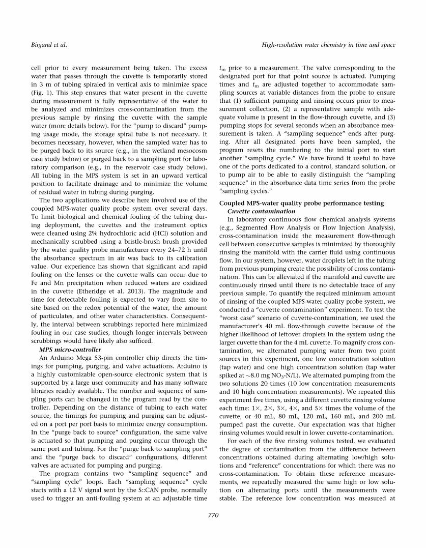
cell prior to every measurement being taken. The excess
water that passes through the cuvette is temporarily stored
in 3 m of tubing spiraled in vertical axis to minimize space
(Fig. 1). This step ensures that water present in the cuvette
during measurement is fully representative of the water to
be analyzed and minimizes cross-contamination from the
previous sample by rinsing the cuvette with the sample
water (more details below). For the “pump to discard” pump-
ing usage mode, the storage spiral tube is not necessary. It
becomes necessary, however, when the sampled water has to
be purged back to its source (e.g., in the wetland mesocosm
case study below) or purged back to a sampling port for labo-
ratory comparison (e.g., in the reservoir case study below).
All tubing in the MPS system is set in an upward vertical
position to facilitate drainage and to minimize the volume
of residual water in tubing during purging.
The two applications we describe here involved use of the
coupled MPS-water quality probe system over several days.
To limit biological and chemical fouling of the tubing dur-
ing deployment, the cuvettes and the instrument optics
were cleaned using 2% hydrochloric acid (HCl) solution and
mechanically scrubbed using a bristle-brush brush provided
by the water quality probe manufacturer every 24–72 h until
the absorbance spectrum in air was back to its calibration
value. Our experience has shown that significant and rapid
fouling on the lenses or the cuvette walls can occur due to
Fe and Mn precipitation when reduced waters are oxidized
in the cuvette (Etheridge et al. 2013). The magnitude and
time for detectable fouling is expected to vary from site to
site based on the redox potential of the water, the amount
of particulates, and other water characteristics. Consequent-
ly, the interval between scrubbings reported here minimized
fouling in our case studies, though longer intervals between
scrubbings would have likely also sufficed.
MPS micro-controller
An Arduino Mega 53-pin controller chip directs the tim-
ings for pumping, purging, and valve actuations. Arduino is
a highly customizable open-source electronic system that is
supported by a large user community and has many software
libraries readily available. The number and sequence of sam-
pling ports can be changed in the program read by the con-
troller. Depending on the distance of tubing to each water
source, the timings for pumping and purging can be adjust-
ed on a port per port basis to minimize energy consumption.
In the “purge back to source” configuration, the same valve
is actuated so that pumping and purging occur through the
same port and tubing. For the “purge back to sampling port”
and the “purge back to discard” configurations, different
valves are actuated for pumping and purging.
The program contains two “sampling sequence” and
“sampling cycle” loops. Each “sampling sequence” cycle
starts with a 12 V signal sent by the S::CAN probe, normally
used to trigger an anti-fouling system at an adjustable time
tm prior to a measurement. The valve corresponding to the
designated port for that point source is actuated. Pumping
times and tm are adjusted together to accommodate sam-
pling sources at variable distances from the probe to ensure
that (1) sufficient pumping and rinsing occurs prior to mea-
surement collection, (2) a representative sample with ade-
quate volume is present in the flow-through cuvette, and (3)
pumping stops for several seconds when an absorbance mea-
surement is taken. A “sampling sequence” ends after purg-
ing. After all designated ports have been sampled, the
program resets the numbering to the initial port to start
another “sampling cycle.” We have found it useful to have
one of the ports dedicated to a control, standard solution, or
to pump air to be able to easily distinguish the “sampling
sequence” in the absorbance data time series from the probe
“sampling cycles.”
Coupled MPS-water quality probe performance testing
Cuvette contamination
In laboratory continuous flow chemical analysis systems
(e.g., Segmented Flow Analysis or Flow Injection Analysis),
cross-contamination inside the measurement flow-through
cell between consecutive samples is minimized by thoroughly
rinsing the manifold with the carrier fluid using continuous
flow. In our system, however, water droplets left in the tubing
from previous pumping create the possibility of cross contami-
nation. This can be alleviated if the manifold and cuvette are
continuously rinsed until there is no detectable trace of any
previous sample. To quantify the required minimum amount
of rinsing of the coupled MPS-water quality probe system, we
conducted a “cuvette contamination” experiment. To test the
“worst case” scenario of cuvette-contamination, we used the
manufacturer’s 40 mL flow-through cuvette because of the
higher likelihood of leftover droplets in the system using the
larger cuvette than for the 4 mL cuvette. To magnify cross con-
tamination, we alternated pumping water from two point
sources in this experiment, one low concentration solution
(tap water) and one high concentration solution (tap water
spiked at �8.0 mg NO3-N/L). We alternated pumping from the
two solutions 20 times (10 low concentration measurements
and 10 high concentration measurements). We repeated this
experiment five times, using a different cuvette rinsing volume
each time: 13, 23, 33, 43, and 53 times the volume of the
cuvette, or 40 mL, 80 mL, 120 mL, 160 mL, and 200 mL
pumped past the cuvette. Our expectation was that higher
rinsing volumes would result in lower cuvette-contamination.
For each of the five rinsing volumes tested, we evaluated
the degree of contamination from the difference between
concentrations obtained during alternating low/high solu-
tions and “reference” concentrations for which there was no
cross-contamination. To obtain these reference measure-
ments, we repeatedly measured the same high or low solu-
tion on alternating ports until the measurements were
stable. The reference low concentration was measured at
Birgand et al. High-resolution water chemistry in time and space
770

0.08 6 0.02 NO3-N mg/L, while the reference high concentra-
tion was measured at 8.02 6 0.02 mg NO3-N/L, for an N con-
centration ratio between the high and low solutions that
ranged between 44 and 100 (Table 1). We quantified the dif-
ferences and the statistical significance between the treat-
ment and reference concentrations using a Welch t-test from
populations of 10 treatment and 10 reference values using R
software (R Core Development Team 2015).
Cross-contamination
For some applications (see below), it may be desirable to
pump and purge water from and to the same point source. In
these cases, some of the droplets from the previous sample
may contaminate the current source during purging. To quan-
tify the magnitude of this type of contamination, we con-
ducted three experiments with three distinct initially high
concentration values (4.65, 6.97, and 8.13 mg NO3-N/L; Fig.
2). In each experiment, low and high concentration solutions
of 500 mL in volume (prepared as described above) were alter-
nately pumped to the water quality probe, the cuvette was
rinsed by 13 its volume as described above, and the water was
purged back to its point sources so that we could measure the
concentration drifts over 30 measurements of each solution
(n 5 60 measurements total). Our expectation was that the
measurements of water pumped from the low and high con-
centrations would increase and decrease, respectively, over
time due to cross-contamination with the previous high and
low solution samples. From each of the six concentration drifts
(i.e., the linear drift over 30 observations measured for both
high and low concentrations in the three experiments; Fig. 2;
Table 2), we calculated the residual volume, Vres, that could
potentially contaminate point sources during each purging
using the following equation:
Vres5Cfinal2Cinitial
Calt2Cinitial
� �:
V
p=2ð Þ (1)
Where Cfinal and Cinitial are the final and initial nitrate
concentrations measured from each concentration drift, Calt
is the concentration of the alternate solution (i.e., for an
upward drift, Calt is the high concentration, and for a down-
ward drift, Calt is the low concentration), V is the volume of
the point source solution, which stayed stable at 500 mL
and (p/2) is the number of measurements per point source
(e.g., 60/2 5 30). Calt was treated as constant and equal to
the average over the 30 purges of the alternate concentra-
tion. We used the global calibration from the S::CAN instru-
ment to calculate the concentration of nitrate in each
measurement.
Concentration computations using the S::CAN probe
Chemometrics algorithms
As noted above, the S::CAN probe measures light absor-
bance on wavelengths ranging from 200 nm to 737.5 nm on
a 2.5 nm resolution. The probe is fitted with algorithms that
interpret the absorbance spectrum to calculate analyte con-
centrations; however, the manufacturer recommends that
the calculated concentrations be locally calibrated with labo-
ratory analyses. For nitrate concentrations within validated
ranges, such calibration may correspond to an offset or slope
change specific to the matrix of water being analyzed
(S::CAN Spectrometer Probe Manual 2011).
Table 1. Nitrate-nitrogen (nitrate-N) concentration values for the reference solutions, p-values quantifying the significance of thedifferences between the treatment and the reference concentrations (Welch t-test on population means) for both high and low con-centration solutions, and 95% confidence intervals (95% CI) of the absolute and relative (expressed in %) difference between thetreatment and the reference concentrations for both high and low nitrate-N concentration solutions. Asterisks denote non-significance.
Reference nitrate-N
concentrations p-values 95% CI
Volume of water used
to rinse the cuvette High Low High Low High Low
1X cuvette vol. 8.02 6 0.02 0.18 6 0.02 <0.0001 <0.0002 (20.26, 20.22)
(23.0%; 22.7%)
(0.22, 0.29)
(122%, 161%)
2X cuvette vol. 8.02 6 0.02 0.18 6 0.02 <0.0001 <0.0001 (20.09, 20.07)
(21.1%; 20.9%)
(0.04,0.10)
(22%, 55%)
3X cuvette vol. 8.02 6 0.02 0.08 6 0.02 <0.0001 <0.0001 (20.09, 20.07)
(21.1%; 20.9%)
(0.05,0.07)
(62%, 88%)
4X cuvette vol. 8.02 6 0.02 0.08 6 0.02 <0.0001 <0.0001 (20.08, 20.06)
(21.0%; 20.7%)
(0.02,0.03)
(25%, 38%)
5X cuvette vol. 7.92 6 0.01 0.08 6 0.02 0.004 0.06* (20.02, 20.00)
(20.2%; 20%)
(20.00,0.01)
(0%, 13%)
*Indicates non-significance.
Birgand et al. High-resolution water chemistry in time and space
771

To examine the concentrations of analytes other than
those with established global S::CAN calibrations (i.e.,
nitrate, DOC, TOC, and turbidity), we used the Partial Least
Square Regression (PLSR) package (Mevik et al. 2011) in the
R statistical framework (R Core Development Team 2015) to
correlate absorbance data with phosphate, iron, and silica,
following the procedure detailed in Etheridge et al. (2014).
Briefly, PLSR is a chemometric technique which reduces the
large number of absorbance measurements from each wave-
length in principal component vectors to best explain mea-
surement variance. This statistical technique is well suited
for situations in which the explanatory variables are highly
autocorrelated, as is expected by absorbance values from
sequential wavelengths. The optimum number of PLSR com-
ponents for each analyte was chosen as the lowest number
of components for which the root mean square error of con-
centration prediction (RMSEP) was at or near its minimum
value.
Results
Performance testing
Cuvette contamination
Our data indicate that cuvette contamination between
the alternating low and high solutions is detectable and sig-
nificant after rinsing the cuvette with 13, 23, 33, and 43
times the cuvette volume for the 40 mL cuvette (as deter-
mined by significant differences between the mean concen-
trations; Table 1). However, after rinsing the cuvette with
five times its volume, no significant differences between the
reference and low concentration solution were observed
(Table 1). While 53 rinsing would be ideal, it requires much
longer pumping times and consequently fewer measure-
ments over time. In our test, the sampling cycle time for 53
rinsing was 270 s, while that of 33 rinsing only lasted 205 s,
i.e., 24% less time. While there was still statistically signifi-
cant cuvette contamination detected for all but 5X rinsing,
in practical terms it may be just as meaningful to evaluate
the absolute difference between the reference and the mea-
sured concentrations. For 23 rinsing, our results show that
high concentrations were underestimated by about 1%
(Table 1). For many applications, this may equate to accept-
able concentration differences or be at the limit of detection.
However, should the precision expectations be very high,
particularly for low concentrations, then 53 rinsing may be
required. For practical purposes, given that the concentra-
tion ratio between consecutive samples is less than 20 in the
vast majority of cases, rinsing the cuvette with 33 its vol-
ume should be sufficient for avoiding cuvette
contamination.
Cross-contamination
Additional care is also needed when the “purge to source”
configuration is used. In this configuration, the 500 mL
point sources became contaminated over time as expected,
i.e., diluted or concentrated by the alternate low or high
samples, respectively. The dilution of the high nitrate solu-
tion and the concentration of the low solution increased as
a function of the concentration difference between the two
solutions: the cross contamination was greatest using a high
nitrate solution initially measured at 8.13 mg NO3-N/L, in
comparison to high N solutions initially measured at 4.65 or
6.97 mg NO3-N/L (Fig. 2).
From the concentration drifts measured, the estimates of
the potentially contaminating residual volume in each
experiment varied from 2.6 mL to 2.9 mL (Table 2). Thus,
when pumping and purging water from and to the same
point source using the manufacturer’s 40 mL flow-through
Fig. 2. Increasing dilution and concentration over time of the original
high and low nitrate-N concentration solutions, respectively, due tocross contamination when pumping from and purging to the samepoint source. Black circles represent measurements of the high nitrate-N
concentration solution and white circles represent measurements of thelow nitrate-N concentration solution after each consecutive purge of
the coupled MPS-water quality probe system. Each of the panels showthe experiment repeated for a high N solution initially measured at (a)4.65 mg NO3-N/L; (b) 6.97 mg. NO3-N/L and (c) 8.13 mg NO3-N/L;
the low N solution for all three experiments was initially measured at0.59 mg NO3-N/L. Note that the y-axes differ among panels.
Birgand et al. High-resolution water chemistry in time and space
772

cell, potentially up to 3 mL of the previous sample can con-
taminate the point source. This suggests that the “purge to
source” configuration should only be used with confidence
in the cases for which the effects of contaminating residual
volume remain undetectable, i.e., the dilution or concentra-
tion would remain small enough to be within the instru-
ment measurement uncertainty, which in our case here was
estimated to be 0.02 mg NO3-N/L of nitrate as the 95% con-
fidence interval from 20 repeated measurements. These con-
ditions can be met when the point source volume is large
compared to the contaminating residual volume and when
the difference in concentrations between consecutive sam-
ples is relatively small. For example, assuming 3 mL of
potentially contaminating volume for two alternating point
sources of 20 L each with concentrations that differ by 2 mg
NO3-N/L, it would take more than 60 consecutive purges to
the point source to detect the effect of cross-contamination.
The number of purges would increase if the effective con-
taminating volume decreased (e.g., by using a smaller vol-
ume flow-through cuvette, such as a smaller volume quartz
flow-through cuvette) or if there was a smaller difference in
concentrations between consecutive measurements. In all
cases, these results suggest that the “purge back to source”
configuration should only be used within the limits defined
here.
Two case studies
Application 1: Using the coupled MPS-water quality probe
system to quantify the effects of water current velocity on
constructed wetland treatment efficiency
Hyporheic advective exchange in wetlands
Nitrate removal processes (e.g., denitrification) in wet-
lands that receive excess nitrate are limited, in part, by the
ability of nitrate to move from the water column to sedi-
ment denitrifying microsites (reviewed by Birgand et al.
2007). In stagnant water, this transport is diffusive in nature
and therefore slow. Many studies conducted in streams have
shown that nitrate exchange between the water column and
underlying substrate (the hyporheic zone), can be greatly
enhanced by advective transport of water into the sediment.
This advective transport can occur as a result of increased
water current velocity above the sediment’s uneven surface or
obstacles above the sediment, such as sand deposits in streams
(e.g., Savant et al. 1987; Thibodeaux and Boyle 1987; Huettel
et al. 1996; Elliott and Brooks 1997; Hutchinson and Webster
1998), or a loose matrix of debris from dead macrophyte stems
deposited onto wetland sediments.
We hypothesized that increasing the current velocity of
water above the sediment bottom in constructed treatment
wetlands would induce advective exchange between the
water column and the sediment, thereby increasing denitrifi-
cation and enhancing treatment efficiency. The implication
is that it may be possible to construct wetlands to be more
efficient in removing nitrogen per unit area by increasing
water current velocity over the sediments.
To test this first hypothesis, we conducted a mesocosm
experiment in which we recirculated water overlying undis-
turbed large sediment cores collected from a wetland at dif-
ferent velocities. We evaluated nitrogen removal (treatment
efficiency) from the kinetics of the decreasing nitrate con-
centration over time in the overlying water. Our second
hypothesis was that the use of the coupled MPS-water quali-
ty probe system would both improve our measurement of
nitrogen removal kinetics and provide information on the
spatial variability of nitrogen removal in replicated wetland
mesocosms.
Experimental set-up and mesocosm description
To create the mesocosms, we collected three undisturbed
whole core wetland samples (56 cm in diameter, 15 cm
deep) by inserting large 30 cm-long PVC rings of the same
diameter into the organic substrate of a riparian wetland
adjacent to eutrophic Rocky Branch stream which receives
pulses of high nitrate concentrations (�2–5 mg NO3-N/L)
and runs through the North Carolina State University cam-
pus (Raleigh, North Carolina, U.S.A.; 3584605000 N, 788400
800 W). To ease insertion of the rings and reduce disturbance
of the cores, a machete blade was used to cut vertically into
the substrate. After the rings were inserted, a 60-cm wide
aluminum blade was used to cut horizontally and provide
support under the cores, which were then excavated and
transferred over 70 cm diameter Plexiglas disks as core
Table 2. Estimates of the apparent contaminating residual volume Vres in mL remaining in the cuvette after a sample that couldpotentially contaminate the consecutive source using the manufacturer’s 40 mL flow-through cuvette when using the “purge back topoint source” configuration.
High concentration source Low concentration source
Initial nitrate-N
concentration
(mg NO3-N/L) Vres (mL)
95% Confidence
intervals
Initial nitrate-N
concentration
(mg NO3-N/L) Vres (mL)
95% Confidence
intervals
4.65 2.89 (2.83, 2.95) 0.89 2.79 (2.76, 2.83)
6.97 2.77 (2.72, 2.81) 0.59 2.64 (2.58, 2.70)
8.13 2.56 (2.53, 2.59) 0.59 2.77 (2.74, 2.80)
Birgand et al. High-resolution water chemistry in time and space
773

bottoms, brought back to the lab, and sealed at the bottom
by pressing the rings against a neoprene seal using
turnbuckles.
We report three experiments that corresponded to three
different water recirculation velocities (0, 3, and 11 cm/s).
Each experiment consisted of three replicated sediment mes-
ocosms and one control mesocosm that did not have any
sediment on its Plexiglas bottom. Ten cm of Rocky Branch
stream water was added to all four mesocosms, which was
recirculated individually in each mesocosm at a stable veloci-
ty throughout the experiment (16.6 L of total water per mes-
ocosm). To compensate for water losses from evaporation,
deionized water was automatically added through a Mariotte
jar system which effectively maintained the water column
height constant. Water velocities were controlled using sub-
merged aquarium pumps, installed parallel to the tangent of
the PVC ring. The intake and outlet valves on the pumps
were opened and closed to create higher or lower velocities,
respectively, in the three different experiments.
The mesocosms were large enough to create the condi-
tions for circular racetrack flumes and 10 cm deep. Flow pat-
terns in racetrack flumes are complicated and involve
advective cells and dead zones at their centers (e.g., Khalili
et al. 1997, 1999; Basu and Khalili 1999). To limit dead
zones, flow in the mesocosm centers was excluded by adding
and centering 20-cm diameter stainless steel cylinders, leav-
ing flow to occur in a circular shape. Velocity values used for
analysis were measured at the center of the cross-section of
the doughnut channel using a Marsh-McBirney Flo-MateTM
(Frederick, Maryland, U.S.A.).
Experimental data collection
We quantified nitrate removal efficiency by measuring
the rate of decreasing nitrate concentrations in the meso-
cosms. We first spiked the water overlaying the sediment
with potassium nitrate to reach 2–3 times the background
nitrate concentrations, which varied between 1.5 and 3.0 mg
NO3-N/L. To reduce nitrate assimilation or release due to
photosynthetically-active vegetation and algae, macrophyte
vegetation in the mesocosms was clipped and all incubations
were conducted in the dark. All cores were incubated at the
same near constant temperature (208C 6 18C) in a controlled
temperature room over 30 h, the length of each of the three
experiments.
During the water recirculation, the coupled MPS-water
quality probe system was used to measure nitrate concentra-
tions on a sampling sequence of every 2.5 min, resulting in
a 10-min sampling cycle or 10-min resolution data for each
of the three treatment mesocosms and the control. The
water intake tubing was placed in the mesocosms’ channel
center, 5 cm above the sediment, with one point source per
mesocosm. The system was configured to pump from and
purge water back to the same mesocosm. Using the 4 mL
quartz cuvette, the contaminating residual volume was
estimated to be no more than 1 mL, and the concentration
difference between consecutive samples was always less than
2 mg NO3-N/L, so that cross-contamination could not be
detected 30 h after the beginning of the experiment.
Nitrate concentrations given by the Spectro::lyserTM were
compared to and corrected by an offset to match laboratory
values for each experiment (details in Horstman 2012). We
removed 8 mL of water from each mesocosm at �12 h fre-
quency for manual nitrate measurements; these samples
were immediately passed through 0.2 lm filters and kept at
48C until analysis on a Lachat Quik-Chem 8000 (Lachat
Instruments, Loveland, Colorado, U.S.A.) following the
Quick-Chem Method 10-115-10-1-B. Between each of the
three different recirculation experiments, all of the overlying
water was siphoned out from each mesocosm, which were
left water-saturated until the next experiment. New stream
water was then added to re-fill the mesocosms, recirculated
at the desired velocity, and spiked with nitrate following the
same procedure.
Nitrate removal rates kinetics
We used the nitrate concentrations measured by the cou-
pled MPS-water quality probe system to estimate nitrate
removal rates. To quantify nitrate uptake or removal rates
(R), i.e., the mass of nitrate removed per projected surface
area per time (e.g., mg NO3-N/m2/d), in stream and wet-
lands, four general kinetics models have been proposed: zero
order rate models (e.g., Horne 1995; Mitsch et al. 2005)
where the rates are independent of the water column nitrate
concentration (i.e., R 5 k, where k is a constant); first order
models (e.g., Stream Solute Workshop 1990; reviewed in Bir-
gand et al. 2007), where the rates are proportional to the
water column nitrate concentrations (i.e., R 5 qC, where q is
the proportionality coefficient otherwise referred to as the
mass transfer coefficient or uptake velocity, and C is the
water column nitrate concentration); efficiency loss models
(O’Brien et al. 2007), where the rates are less than propor-
tional to the water column nitrate concentrations (i.e.,
R 5 cCa, where a is less than 1 and higher than 0, and c is
the mass transfer coefficient); and Michaelis-Menten models
(i.e., R5 Rmax:C0
Ks1 C0, where Rmax is the maximum nitrate removal
rate, C0 is the initial nitrate concentration, and Ks is the half
saturation constant; e.g., Bernot and Dodds 2005).
For the simplicity of its application, and possibly also due
to the lack of data, the first order model is the one most
often used in streams (e.g., Smith et al. 1997; Alexander
et al. 2000) and wetlands (e.g., Kadlec and Wallace 2009).
Here, we used the high-resolution nitrate data collected by
the coupled MPS-water quality probe system to compare the
performances of the first order model to those of the effi-
ciency loss and the Michaelis-Menten models (Fig. 4; Table
4) by fitting the models to the measured nitrate concentra-
tions and removal rates using the nonlinear least square
method package nls in the R software.
Birgand et al. High-resolution water chemistry in time and space
774

Mesocosm experimental results
We observed that nitrate removal is variable but increases
with current velocity. Nitrate concentration decreases measured
for 0, 3, and 11 cm/s water current velocities for the three meso-
cosm replicates (rep1, rep2, and rep3) and the control by the
coupled MPS-water quality probe system are illustrated in Fig. 3
(data for rep2 at 3 cm/s were discarded because the water intake
became clogged during the experiment). Nitrate concentrations
for the control remained constant over time, indicating no
detectable removal. Nitrate removal, indicated by the slope of
the concentration time series in Fig. 3, increased with increasing
velocity, supporting our initial hypothesis.
However, while nitrate removal rates for rep2 and rep3
had similar responses to increased velocity, the response of
rep1 at 11 cm/s yielded much lower rates. After careful visual
inspection, the rep1 sediment surface appeared “smooth”
compared to the other two treatment mesocosm sediment
surfaces, suggesting that the sediment pores and irregulari-
ties clearly visible at the sediment surface for rep2 and rep3
may have been clogged by particles resuspended by water
current during the experiments. The smooth surface in rep1
may have dramatically decreased the advective exchange
that is induced by velocity over porous sediment irregulari-
ties (e.g., Hutchinson and Webster 1998; Marion et al. 2002;
Packman and Salehin 2003; Salehin et al. 2003; Packman
et al. 2004), hence reducing the ability for nitrate to reach
denitrification microsites. Our experiment thus suggests that
moving water above uneven, porous, and organic con-
structed wetland sediments may increase the ability of water
column nitrate to penetrate into the reactive sediment,
where it may be removed.
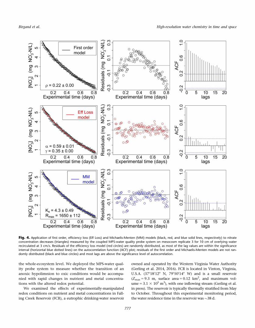
Our results show that the first order rate kinetic model
appears inappropriate. It does not fit the observed data well
(Fig. 4), as the model residuals are not randomly distributed.
This is confirmed by the autocorrelation function (ACF),
which shows that the residuals are significantly auto-
correlated. In contrast, the efficiency loss model provides the
best fit to the data as the model residuals are randomly distrib-
uted and not significantly auto-correlated for all experiments
and replicates. The Michaelis-Menten model also generally
performs well, although there are two cases in which the mod-
el residuals are not randomly distributed and are significantly
auto-correlated (Fig. 4; Table 3). Similar to our observations,
O’Brien et al. (2007) have shown that the efficiency loss model
fitted stream nitrate removal better than the first order or the
Michaelis-Menten models. Furthermore, the nitrate concen-
tration time series in Fig. 3 did not exhibit any linear patterns,
which ruled out the use of zero order models.
Table 3. Summary statistics of the model goodness of fit (auto-correlation function (ACF): Yes, when residuals show significantauto-correlation, No, otherwise) and model parameter values (6 standard error from the nonlinear regression parameter estimate) forthe first order, efficiency loss (Eff Loss), and Michaelis-Menten models; estimated time it would take to lower nitrate concentrationsfrom 5 mg to 0.25 mg nitrate-nitrogen (NO3-N)/L using the first order and efficiency loss models; and the percentage differencebetween the estimated times from the Eff loss and first order models.
0 cm/s 3 cm/s 11 cm/s
Rep1 Rep2 Rep3 Rep1 Rep3 Rep1 Rep2 Rep3
First order
model
ACF Yes Yes Yes Yes Yes Yes Yes Yes
q
(m/d)
0.15 6 0.00 0.19 6 0.00 0.14 6 0.00 0.27 6 0.01 0.22 6 0.002 0.28 6 0.002 1.02 6 0.02 1.25 6 0.02
Efficiency loss
model
ACF No No No No No No No No
c
(m/d)
0.26 6 0.01 0.29 6 0.01 0.35 6 0.02 0.21 6 0.01 0.35 6 0.01 0.37 6 0.001 1.23 6 0.04 1.54 6 0.03
A 0.38 6 0.07 0.52 6 0.04 0.22 6 0.04 0.63 6 0.02 0.59 6 0.02 0.75 6 0.02 0.77 6 0.04 0.81 6 0.01
Michaelis-
Menten
model
ACF Yes No No No Yes No No No
Ks
(mg NO3-N/L)
2.28 6 0.74 2.04 6 0.41 0.87 6 0.23 0.64 6 0.05 4.30 6 0.49 8.79 6 0.68 3.98 6 0.29 11.1 6 0.75
Rmax
(mg N/m2/d)
733 6 116 856 6 82 578 6 36 972 6 15 1650 6 112 3397 6 191 6142 6 304 17106 6 945
Time to lower
[NO3-N]
from 5.0 to
0.25 mg
NO3-N/L
(days)
First order 2.00 1.54 2.06 0.94 1.34 1.06 0.29 0.28
Eff loss 1.43 1.18 1.17 0.65 0.96 0.84 0.25 0.19
Percentage difference in time estimate 40% 30% 77% 45% 39% 25% 16% 42%
Birgand et al. High-resolution water chemistry in time and space
775

Without the coupled MPS-water quality probe system,
nitrate concentrations would have been obtained from man-
ual samples of the water in the laboratory, which would
have substantially reduced the temporal resolution of sam-
pling points for logistical reasons. Using traditional sampling
methods (e.g., by collecting water from the mesocosms �5
times over 24 h for nitrate analysis in the laboratory), it
would have been impossible to show that the first order
model was inappropriate, or to show that the efficiency loss
model was significantly better in calculating nitrate removal.
Using both the first order and efficiency loss models (the
worst-fitting and best-fitting models tested, respectively), we
calculated the estimated time it would take to decrease
nitrate concentration from 5 to 0.25 mg NO3-N/L (typical
values representing high and low nitrate concentrations
observed in constructed wetlands; Kadlec and Wallace 2009),
for each replicate and each experiment (Table 3). Our results
show that the first order model, which is the most widely
used, tends to overestimate the time it would take to remove
nitrate by �30–40%, compared to the efficiency loss model,
which fits the data much better. These results suggest that
the common approach to predicting wetland nitrate removal
using the first order model may be too conservative and may
significantly under-predict removal efficiency.
Moreover, our data also suggest that increasing water
movement in wetlands greatly increases nitrate removal
efficiency from its default stagnant state (Table 3). Using the
efficiency loss model results in Table 4, our data indicate
that nitrate removal processes may be occurring four to six
times more quickly when the water velocity is increased
from 0 to 11 cm/s. Initial removal rates reached up to �6 g/
m2/d, which correspond to the upper range of rates reported
in treatment wetlands (Kadlec and Wallace 2009). Interest-
ingly, the exponent in the efficiency loss model also
increased with increasing velocity, and so do the Rmax val-
ues. Increasing water velocity could therefore decrease the
duration of time needed for nitrate removal processes in
constructed wetlands. In summary, the use of the coupled
MPS-water quality probe system in this application has
shown, potentially for the first time, that the common first
order rate kinetic approach is too conservative for estimating
nitrate removal and that recirculating water in wetlands is
crucial for stimulating nitrate removal processes.
Application 2: Whole-ecosystem responses to hypolim-
netic oxygenation in a reservoir
Managers and utilities are increasingly using oxygenation
systems to improve water quality in lakes and reservoirs used
for drinking water (Singleton and Little 2006; Gerling et al.
2014, 2016). While oxygenation has been shown to success-
fully decrease soluble nutrient and metal concentrations
over day to week time scales, the effects of oxygenation on
shorter (minute) time scales remain unknown, especially at
Fig. 3. The decrease in nitrate-N concentrations over time for three mesocosm experiments with different recirculation velocities (0, 3, and 11 cm/s).
Each experiment consisted of three large constructed wetland sediment core replicates (denoted as rep1, rep2, and rep3) and one control with nosediment; in the left panel, data are organized as a function of the velocity treatments and in the right panel, as a function of the replicates. Data forrep2 of the 3 cm/s experiment were omitted because the water intake became clogged during the experiment.
Birgand et al. High-resolution water chemistry in time and space
776
the whole-ecosystem level. We deployed the MPS-water qual-
ity probe system to measure whether the transition of an
anoxic hypolimnion to oxic conditions would be accompa-
nied with rapid changes in nutrient and metal concentra-
tions with the altered redox potential.
We examined the effects of experimentally-manipulated
redox conditions on nutrient and metal concentrations in Fall-
ing Creek Reservoir (FCR), a eutrophic drinking-water reservoir
owned and operated by the Western Virginia Water Authority
(Gerling et al. 2014, 2016). FCR is located in Vinton, Virginia,
U.S.A. (3781801200 N, 7985001400 W) and is a small reservoir
(Zmax 5 9.3 m, surface area 5 0.12 km2, and maximum vol-
ume 5 3.1 3 105 m3), with one inflowing stream (Gerling et al.
in press). The reservoir is typically thermally stratified from May
to October. Throughout this experimental monitoring period,
the water residence time in the reservoir was�38 d.
Fig. 4. Application of first order, efficiency loss (Eff Loss) and Michaelis-Menten (MM) models (black, red, and blue solid lines, respectively) to nitrateconcentration decreases (triangles) measured by the coupled MPS-water quality probe system on mesocosm replicate 3 for 10 cm of overlying water
recirculated at 3 cm/s. Residuals of the efficiency loss model (red circles) are randomly distributed, as most of the lag values are within the significanceinterval (horizontal blue dotted lines) on the autocorrelation function (ACF) plot; residuals of the first order and Michaelis-Menten models are not ran-
domly distributed (black and blue circles) and most lags are above the significance level of autocorrelation.
Birgand et al. High-resolution water chemistry in time and space
777
In 2012, a side-stream supersaturation (SSS) oxygenation sys-
tem was deployed in FCR to increase hypolimnetic oxygen con-
centrations. The SSS pumps hypolimnetic water from 8.5 m
depth onshore to an oxygen contact chamber, injects concen-
trated oxygen gas under high pressure, and then returns the
super-saturated oxygenated water at the same temperature and
depth to the hypolimnion (see Gerling et al. 2014 for more
details on the engineering design of the system). The oxygenat-
ed water is ejected from the SSS via eductor nozzles into the
hypolimnion under pressure, resulting in a uniformly-mixed
hypolimnion with similar oxygen concentrations above and
below the SSS distribution header. Initial operation of the SSS
demonstrates that the system is able to successfully increase oxy-
gen concentrations in the water column while maintaining
thermal stratification (Gerling et al. 2014). Once activated, the
SSS increases oxygen concentrations in the bulk hypolimnion
through mixing via eductor nozzles within an hour.
We intensively monitored FCR with the MPS-water quali-
ty probe system described in this article for 9 d in summer
2014. The system was deployed on a permanent platform
built 1.5 m above the water’s surface at the deepest site of
the reservoir. Ten ports of the multiplexer were used pump-
ing water from nine depths (0.1, 0.8, 1.6, 2.8, 3.8, 5, 6.2, 8.0,
and 9.0 m, corresponding to the intake depths for the water
treatment plant), while the tenth port was used to pump air
for reference purposes. Water was not purged back to its
source, but was purged to the tenth port, from which series
of manual samples were taken for laboratory analyses. Pump
timings were adjusted to account for water in the tubing
from the previous cycle to be pumped out, and for “new”
water to be pumped in the cuvette for at least the equivalent
of 3X cuvette volumes for rinsing and such that the tubing
coil past the cuvette be filled with new water for manual
sampling purposes. As a result, in addition to cuvette rins-
ing, the immersed tubing was thus rinsed by 2.5 to 10X the
tubing’s volume of new water, depending on the tubing
length. The sampling sequence for each port lasted 3 min,
for a final sampling cycle time resolution of 30 min at each
of the nine depths.
As the total absorbance was expected to be low, the
S::CAN spectrometer was outfitted with the 40 mL manufac-
turer cuvette modified as a flow-through cell to maintain
35 mm measurement path length. The MPS-water quality
probe system continuously cycled from the nine depths
throughout the monitoring period, except for 15 min breaks
every second or third day to clean the cuvette and the optics
with cotton swabs soaked in 2% HCl to prevent metal pre-
cipitate from oxidizing on the sensor.
From manual samples described earlier, we measured a
suite of chemistry response variables from the sampled reser-
voir water. Water samples from each of the nine depths were
collected for metals and nutrient analyses on 29 June (both
1 h before and 1 h after the SSS was activated), 30 June, and
07 July, providing n 5 36 calibration data points total. On
each sampling day, we filtered water from each depth
through GF/F Whatman filters (0.7 lm pore size) into acid-
washed bottles, which were frozen until analysis. These sam-
ples were analyzed for nitrate-nitrite (NO3-NO2), and phos-
phate (PO324 ) on a Lachat following the Quik-Chem Method
10-115-10-1-B. Second, collected water from each depth was
used to measure dissolved fractions (filtered through 0.4 lm
pore size filters) of Si and Fe using a Thermo Electron X-
Series inductively coupled plasma mass spectrometer (ICP-
MS) per Standard Method 3125-B (APHA, AWWA, and WEF
1998). ICP-MS samples and calibration samples were pre-
pared in a matrix of 2% nitric acid by volume.
We began the experiment in the evening of 27 June 2014,
when the SSS was deactivated and the hypolimnion was
anoxic. At 11:00 on 29 June 2014, the SSS was activated to
continuously add 25 kg O2/day to the hypolimnion. We
monitored the increase in hypolimnetic oxygen and its
effects on metals and nutrient concentrations in the water
column for 7 d at a 30 min resolution, until 06 July 2014.
The changes in temperature, dissolved oxygen, and chloro-
phyll a, and turbidity with depth are reported elsewhere
(Gerling et al. 2016).
Co-variability between concentrations and “color
matrix” of water
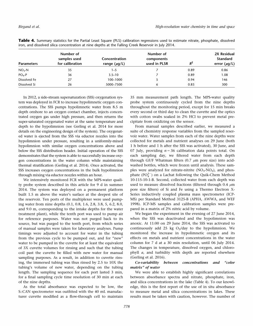
We were able to establish highly significant correlations
between absorbance spectra and nitrate, phosphate, iron,
and silica concentrations in the lake (Table 4). To our knowl-
edge, this is the first report of the use of in situ absorbance
to measure metal and silica concentrations in lakes. These
results must be taken with caution, however. The number of
Table 4. Summary statistics for the Partial Least Square (PLS) calibration regressions used to estimate nitrate, phosphate, dissolvediron, and dissolved silica concentration at nine depths at the Falling Creek Reservoir in July 2014.
Parameters
Number of
samples used
for calibration
Concentration
range (lg/L)
Number of
components
used in PLSR R2
2X Residual
Standard
error (lg/L)
NO3-N 35 1–5 7 0.89 0.86
PO4-P 36 3.5–10 7 0.89 1.08
Dissolved Fe 27 100–1000 5 0.94 146
Dissolved Si 26 5000–7500 6 0.83 300
Birgand et al. High-resolution water chemistry in time and space
778

samples for calibration is relatively small (n 5 36), and the
number of components used to obtain PLSR regressions was
higher than 10% of the number of calibrating samples,
which has been suggested as a potential guideline for PLSR
(Mevik et al. 2011). In addition, the measurement uncertain-
ties in elemental concentrations calculated for the water
quality probe (reported in Table 4), are larger than those
generally accepted in the laboratory. Despite these uncer-
tainties, however, the general trends we observed in elemen-
tal concentrations through the water column in response to
oxygenation were robust to the number of components used
in the PLSR regressions (data not shown).
We detected large fluctuations in dissolved Fe and Si con-
centrations that coincided with the shift in redox potential
upon the initiation of oxygenation. The thermocline depth
located at 4 m (Gerling et al. 2016) provides a sharp contrast
to epilimnetic and hypolimnetic conditions. The activation
of oxygenation at midday on 29 June 2014 (vertical white
lines in Fig. 5) is accompanied with rapid changes in the
hypolimnion, particularly at the reservoir sediments, where
dissolved Fe and Si concentrations decrease within a few
hours of oxygenation. Our data suggest that the reservoir
sediments seemed to have been a hot spot for anoxic release
of Fe prior to oxygenation. Interestingly, our results suggest
Fig. 5. Concentration variations of dissolved PO324 , Fe, and Si in Falling Creek Reservoir as a function of depth and time, obtained from 30-min data
for nine depths using the coupled MPS-water quality probe, before and after oxygenation of the hypolimnion (vertical white line).
Birgand et al. High-resolution water chemistry in time and space
779
that there may be diel concentration patterns and large con-
centration changes occurring spatially and in time through-
out the water column. The cause of these diel changes is
unknown, but may be related to light availability in the
hypolimnion, as the oxygen addition rate was constant
throughout the oxygenated monitoring period. Diel shifts in
dissolved organic matter and other elements have also been
measured in other lentic water bodies (e.g., Watras et al.
2015, 2016), which have been attributed to a suite of biogeo-
chemical processes. Throughout the experimental period,
the compensation depth was estimated to be �7.6 m from
Secchi disk measurements, indicating that light was able to
penetrate through most of the hypolimnetic volume, which
was substantially mixed during oxygenation.
Although nitrate is known to absorb light in the 220–
230 nm range (Suzuki and Kuroda 1987; Crumpton et al.
1992), the concentration level observed in the reservoir (1–5
lg N/L; Table 3), is lower than the instrument detection and
resolution limits. We thus believe that not only for nitrate
but for all four parameters reported here, the highly signifi-
cant PLSR regressions are evidence of co-variability between
the absorbance spectra, or the “color matrix” of the water,
and parameter concentrations. Etheridge et al. (2014) pro-
posed the same explanation when monitoring a brackish salt
marsh in North Carolina. We highly recommend future test-
ing and validation for using absorbance data as a surrogate
to measure a large suite of parameters, as this method holds
great promise for measuring a wide range of elements in situ
and at high-frequency temporal resolution. The relatively
buffered variations of hydrological conditions in reservoirs
and lakes, compared to those in streams and rivers, suggest
that lentic waterbodies may be good candidates for deriving
correlations between the color matrix of water and chemical
concentrations. In summary, the use of the coupled MPS-
water quality probe system in this application has shown
minute-resolution changes in the concentrations of elements
that have heretofore never been measured in situ in response
to altered redox conditions, as well as large diel shifts in
multiple elements occurring in the absence of changes in
redox.
Discussion and conclusions
Until very recently, one could obtain high spatial resolu-
tion in water quality variables over a short period (e.g., one
day) by sampling many locations manually or using sam-
pling instruments to collect samples at multiple depths (e.g.,
Morsy 2011). Alternatively, researchers could obtain high
temporal resolution using automatic samplers or using con-
tinuous sensors. Thus, high resolution was achievable either
in space or in time, but almost never together. The increas-
ing availability of in situ high frequency water quality probes
is revolutionizing water quality monitoring, and more
importantly, has the potential to substantially advance our
understanding of aquatic biogeochemistry. Our coupled
MPS-water quality probe system presented here is able to
extend temporal high-frequency capabilities to a greater spa-
tial resolution, permitting up to 12 additional measurements
from nearby sites or replicated units. The results of the per-
formance testing have shown that when the coupled MPS-
water quality probe system is used within the limits defined
in this article, it can provide reliable high-frequency meas-
urements for a variety of different elements. We note that
combined resolution in space and in time has also been
achieved in lentic ecosystems using commercially available
in situ vertical profilers, which automatically sample water
quality variables with sensors at multiple depths in a profile
(e.g., YSI Environmental 2006a,b). These systems have specif-
ically been designed for water bodies several meters deep,
while our system has been designed for these and other uses.
Observing variability at new scales
Continuous high-frequency water quality data at a single
point in a watershed enables capturing rare events (“hot
moments,” McClain et al. 2003) that have a disproportional
impact on nutrient and material fluxes. Our coupled MPS-
water quality probe system opens the possibility to detect
not just hot moments (temporal variability) but also identify
“hot spots” (spatial variability) in the landscape (e.g.,
McClain et al. 2003; Vidon et al. 2010). Consequently, we
can now observe biogeochemical processes that are linked in
time and space. The power of the system for detecting high-
frequency fluxes at multiple sites or depths was particularly
apparent in the reservoir application, when a hot moment
occurred in response to a sudden change in the redox condi-
tions in the hypolimnion. After the initiation of oxygena-
tion, high dissolved Fe concentrations at the anoxic
sediments decreased by a factor of two, likely due to precipi-
tation in increasingly oxic conditions. The slight peak of Fe
at the sediments a few hours after oxygenation began is like-
ly due to the SSS’s mixing of the hypolimnion, entraining
water with high dissolved Fe concentrations from the sedi-
ments to higher depths in the water column, prior to an
overall decrease in concentrations.
Furthermore, the MPS-water quality probe system also
revealed diel fluctuations of nutrient and metal concentra-
tions synchronized in the epilimnion and hypolimnion,
which has been observed in other aquatic systems (e.g.,
Pellerin et al. 2009, 2012; Nimick et al. 2011; Cohen et al.
2012, 2013; Snyder and Bowden, 2014; Watras et al. 2015).
Silica concentrations peak during early afternoons at the
thermocline, while Fe concentrations are at their lowest at
the same time in the epilimnion, which may be due to auto-
trophic and heterotrophic immobilization. By comparison,
while dissolved Fe and Si concentrations appear to vary
almost by a factor of two at every depth over 24 h, the diel
fluctuations of phosphate were not as large. Phosphate con-
centrations temporarily increased after oxygenation, possibly
Birgand et al. High-resolution water chemistry in time and space
780

associated with increased mineralization of organic matter in
the water column. Without additional data on the microbial
and phytoplankton dynamics in the reservoir, we are unable
to identify the mechanisms responsible for these diel cycles,
but hypothesize that they may be due to a combination of
internal waves as well as biological uptake and mineraliza-
tion. We do not rule out, however, that the apparent diel
fluctuations may result, in part, from an artifact of the co-
variability between the color matrix, which may vary on a
diel basis, and the elemental concentrations. Observing both
large amplitude (e.g., for Fe and Si,�15% change from diel
minimum to maximum values) and small amplitude (e.g.,
for PO324 ;�8% change from diel minimum to maximum val-
ues) diel fluctuations does suggest, however, that these fluc-
tuations cannot only result from a methodological artifact.
Overall, these results highlight how dynamic freshwater bio-
geochemical cycles may be in lentic systems, as well as their
sensitivity to changes in redox potential.
The coupled MPS-water quality probe system also eluci-
dated some of the spatial variability of nitrate removal in
constructed wetlands in the mesocosm experiment. The abil-
ity of the system to collect high-frequency (10-min) resolu-
tion data from each sediment site revealed the sensitivity of
nitrate removal processes to water current velocity, as a
result of increased advective exchange between the water
column and the wetland sediment substrate. The positive
response of nitrate removal to current velocity suggests that
reported values in microcosms and mesocosm experiments
for wetland, stream, lake and estuarine sediments in the lit-
erature (e.g., reviewed by Seitzinger 1988; Birgand et al.
2007) may not readily be comparable, as recirculation veloci-
ty is rarely taken into account or reported.
Finally, our high-frequency data also revealed that nitrate
removal kinetics did not follow the traditionally accepted
first order rate model: applying this traditional model to our
data significantly underestimated nitrate removal efficiency.
This conclusion would not have been possible without the
coupled MPS-water quality probe system, which substantiat-
ed this observation in three different experiments and repli-
cated mesocosms.
System limitations and opportunities
We note that the MPS-water quality probe system is flexi-
ble in deployment applications and could be coupled with
any water quality probe collecting data at the minute scale,
not just the S::CAN Spectro::lyserTM. In the applications we
present here, it should be noted that the S::CAN probe could
not be continuously deployed for more than 3 d before the
memory of the instrument was full. In both mesocosm and
reservoir applications, the probe saved>200 absorbance val-
ues every 3 min, requiring data to be downloaded every
third day. This limitation of the water quality probe should
be quickly addressed by the manufacturer, however. The sec-
ond limitation is the fouling of the optics or within the
cuvette. In the two applications shown, overlying water in
the mesocosm experiment and hypolimnion in the reservoir
was anoxic prior to pumping into the system. The sudden
contact of reduced water with air in the cuvette created the
conditions for metal oxidation, the precipitate of which par-
tially coated the optics or the cuvette walls through time
(Etheridge et al. 2013). These had to be cleaned regularly, at
least every 24–72 h, using a 2% HCl solution. A third limita-
tion is electrical power, which can be alleviated with the use
of solar panel to recharge batteries.
Despite its imperfections, we believe that the coupled
MPS-water quality probe system offers enormous potential
and flexibility for the study of aquatic biogeochemical pro-
cesses. The overall cost of materials for the MPS system
presented in this article was less than $2,500 USD in 2013
(not including the cost of the water quality probe or the
time to assemble the parts). In sum, this system is very
affordable for expanding the capabilities of one water qual-
ity probe to collect data at 12 sites, especially in compari-
son to purchasing 11 additional water quality probes. Most
importantly, our system is well suited to capture processes
linked in space and in time, especially the linkage between
“hot spots” and “hot moments” (McClain et al. 2003;
Vidon et al. 2010). As our understanding of biogeochemi-
cal hotspots and hot moments advances, we anticipate the
deployment of similar systems across a diversity of
ecosystems.
References
Alexander, R. B., R. A. Smith, and G. E. Schwarz. 2000. Effect of
stream channel size on the delivery of nitrogen to the Gulf
of Mexico. Nature 403: 758–761. doi:10.1038/35001562
APHA, AWWA, and WEF (American Public Health Associa-
tion, American Water Works Association, and Water Envi-
ronment Federation). 1998. Standard methods for
examination of water and wastewater, 20th ed. APHA.
Basu, A. J., and A. Khalili. 1999. Computation of flow
through a fluid-sediment interface in a benthic chamber.
Phys. Fluids 11: 1395–1405. doi:10.1063/1.870004
Bernot, M. J., and W. K. Dodds. 2005. Nitrogen retention,
removal and saturation in lotic ecosystems. Ecosystems 8:
442–453. doi:10.1007/s10021-003-0143-y
Birgand, F., R. W. Skaggs, G. M. Chescheir, and J. W.
Gilliam. 2007. Nitrogen removal in streams of agricultural
catchments—a literature review. Crit. Rev. Environ. Sci.
Technol. 37: 381–487. doi:10.1080/10643380600966426
Birgand, F., C. Faucheux, G. Gruau, B. Augeard, F. Moatar,
and P. Bordenave. 2010. Uncertainties in assessing annual
nitrate loads and concentration indicators: Part 1. Impact
of sampling frequency and load estimation algorithms.
Trans. ASABE 53: 437–446. doi:10.13031/2013.29584
Chapin, T. P., J. M. Caffrey, H. W. Jannasch, L. J. Colletti, J.
C. Haskins, and K. S. Johnson. 2004. Nitrate sources and
Birgand et al. High-resolution water chemistry in time and space
781

sinks in Elkhorn Slough, California: Results from long-
term continuous in situ nitrate analyzers. Estuaries 27:
882–894. doi:10.1007/BF02912049
Cohen, M. J., J. B. Heffernan, A. Albertin, and J. B. Martin.
2012. Inference of riverine nitrogen processing from lon-
gitudinal and diel variation in dual nitrate isotopes. J.
Geophys. Res. 117: G01021. doi:10.1029/2011JG001715.
Cohen, M. J., M. J. Kurz, J. B. Heffernan, J. B. Martin, R. L.
Douglass, C. R. Foster, and R. G. Thomas. 2013. Diel
phosphorus variation and the stoichiometry of ecosystem
metabolism in a large spring-fed river. Ecol. Monogr. 83:
155–176. doi:10.1890/12-1497.1
Crumpton, W. G., T. M. Isenhart, and P. D. Mitchell. 1992.
Nitrate and organic N analyses with second-derivative
spectroscopy. Limnol. Oceanogr. 37: 907–913. doi:
10.4319/lo. 1992.37.4.0907.
Elliott, A. H., and N. H. Brooks. 1997. Transfer of nonsorbing
solutes to a streambed with bed forms: Laboratory experi-
ments. Water Resour. Res. 33: 137–151. doi:10.1029/
96WR02783
Etheridge, J. R., F. Birgand, M. R. Burchell, II, and B. T.
Smith. 2013. Addressing the fouling of in-situ UV-Visual
spectrometers used to continuously monitor water quality
in brackish tidal marsh waters. J. Environ. Qual. 42:
1896–1901. doi:10.2134/jeq2013.02.0049
Etheridge, J. R., F. Birgand, J. A. Osborne, C. L. Osburn, M.
R. Burchell, II, and J. Irving. 2014. Using in situ
ultraviolet-visual spectroscopy to measure nitrogen, car-
bon, phosphorus, and suspended solids concentrations at
a high frequency in a brackish tidal marsh. Limnol. Oce-
anogr.: Methods 12: 10–22. doi:10.4319/lom.2014.12.10
Gerling, A. B., R. G. Browne, P. A. Gantzer, M. H. Mobley, J. C.
Little, and C. C. Carey. 2014. First report of the successful oper-
ation of a side stream supersaturation hypolimnetic oxygena-
tion system in a eutrophic, shallow reservoir. Water Res. 67:
129–143. doi:10.1016/j.watres.2014.09.002
Gerling, A. B., Z. W. Munger, J. P. Doubek, K. D. Hamre, P.
A. Gantzer, J. C. Little, and C. C. Carey. 2016. Whole-catch-
ment manipulations of internal and external loading reveal
the sensitivity of a century-old reservoir to hypoxia. Ecosys-
tems. 19:555–571. DOI:10.1007/s10021-015-9951-0
Hensley, R. T., M. J. Cohen, and L. V. Korhnak. 2015.
Hydraulic effects on nitrogen removal in a tidal spring-fed
river. Water Resour. Res. 51: 1443–1456. doi:10.1002/
2014WR016178
Horne, A. J. 1995. Nitrogen removal from waste treatment
pond or activated sludge plan effluents with free-surface
wetlands. Water Sci. Technol. 31: 341–351. doi:10.1016/
0273-1223(95)00530-Z
Horstman, M. 2012. Wetland nitrate dissipation capacity
enhancement via increased sediment interfacial nitrate
transport. M.S. thesis. North Carolina State Univ.
Huettel, M., W. Ziebis, and S. Forster. 1996. Flow-induced
uptake of particulate matter in permeable sediments.
Limnol. Oceanogr. 41: 309–322. doi:10.4319/lo.1996.41.
2.0309
Hutchinson, P. A., and I. T. Webster. 1998. Solute uptake in
aquatic sediments due to current–obstacle interactions. J.
Environ. Eng. 124: 419–426. doi:10.1061/(ASCE)0733-
9372(1998)
Kadlec, R. H., and S. D. Wallace. 2009. Treatment wetlands,
2nd ed, 182, 395, 472 p. CRC Press.
Khalili, A., A. J. Basu, and M. Huettel. 1997. A non-Darcy
model for recirculating flow through a fluid-sediment
interface in a cylindrical container. Acta Mech. 123: 75.
doi:10.1007/BF01178402
Khalili, A., A. J. Basu, U. Pietrzyk, and M. Raffel. 1999. An
experimental study of recirculating flow through fluid-
sediment interfaces. J. Fluid Mech. 383: 229. doi:10.1017/
S0022112098003942
Marion, A., M. Bellinello, I. Guymer, and A. I. Packman.
2002. Effect of bed form geometry on the penetration of
nonreactive solutes into a streambed. Water Resour. Res.
38: W1209. doi:10.1029/2001WR000264
McClain, M. E., and others. 2003. Biogeochemical hot spots
and hot moments at the interface of terrestrial and aquat-
ic ecosystems. Ecosystems 6: 301–312. doi:10.1007/
s10021-003-0161-9
Mevik, B., R. Wehrens, and K. H. Liland. 2011. pls: Partial
least squares and principal component regression. R pack-
age 2.3- 0. Available from http://CRAN.R-project.org/pack-
age5pls. doi:10.18637/jss.v018.i02
Mitsch, W. J., J. W. Day, Jr., L. Zhang, and R. R. Lane. 2005.
Nitrate-nitrogen retention by wetlands in the Mississippi
River Basin. Ecol. Eng. 24: 267–278. doi:10.1016/
j.ecoleng.2005.02.005
Morsy, F. M. 2011. A simple approach to water and plankton
sampling for water microbiological and physicochemical
characterizations at various depths in aquatic ecosystems.
Int. J. Limnol. 47: 65–71. doi:10.1051/limn/2010032
Nimick, D. A., C. H. Gammons, and S. R. Parker. 2011. Diel
biogeochemical processes and their effect on the aqueous
chemistry of streams: A review. Chem. Geol. 283: 3–17.
doi:10.1016/j.chemgeo.2010.08.017
O’Brien, J. M., W. K. Dodds, K. C. Wilson, J. N. Murdock,
and J. Eichmiller. 2007. The saturation of cycling in Cen-
tral Plains streams: 15N experiments across a broad gradi-
ent of nitrate concentrations. Biogeochemistry 84: 31–49.
doi:10.1007/s10533-007-9073-7
Packman, A. I., and M. Salehin. 2003. Relative roles of
stream flow and sedimentary conditions in controlling
hyporheic exchange. Hydrobiologia 494: 291–297. doi:
10.1023/A:1025403424063
Packman, A. I., M. Salehin, and M. Zaramella. 2004.
Hyporheic exchange with gravel beds: Basic hydrodynam-
ic interaction and bedform-induced advective flows.
J. Environ. Eng. 130: 647–656. doi:10.1061/(ASCE)0733-
9429(2004)
Birgand et al. High-resolution water chemistry in time and space
782

Pellerin, B. A., and others. 2009. Assessing the sources and
magnitude of diurnal nitrate variability in the San Joa-
quin River (California) with an in situ optical nitrate sen-
sor and dual nitrate isotopes. Freshw. Biol. 54: 376–387.
doi:10.1111/j.1365-2427.2008.02111.x
Pellerin, B. A., J. F. Saraceno, J. B. Shanley, S. D. Sebestyen,
G. R. Aiken, W. M. Wollheim, and B. A. Bergamaschi.
2012. Taking the pulse of snowmelt: In situ sensors reveal
seasonal, event and diurnal patterns of nitrate and dis-
solved organic matter variability in an upland forest
stream. Biogeochemistry 108: 183–198. doi:10.1007/
s10533-011-9589-8
R Core Development Team. 2015. R: A language and envi-
ronment for Statistical Computing. Available from http://
www.R-project.org.
Rieger, L., G. Langergraber, and H. Siegrist. 2006. Uncertain-
ties of spectral in situ measurements in wastewater using
different calibration approaches. Water Sci. Technol. 53:
187–198. doi:10.2166/wst.2006.421.
Salehin, M., A. I. Packman, and A. W€orman. 2003. Compari-
son of transient storage in vegetated and unvegetated
reaches of a small agricultural stream in Sweden: Seasonal
variation and anthropogenic manipulation. Adv. Water
Res. 26: 951–964. doi:10.1016/S0309-1708(03)00084-8
Savant, S. A., D. D. Reible, and L. J. Thibodeaux. 1987. Con-
vective transport within stable river sediments. Water
Resour. Res. 23: 1763–1768. doi:10.1029/WR023i009
p01763
S::CAN Spectrometer Probe V2. 2011. User Manual. Vienna,
Austria.
Seitzinger, S. P. 1988. Denitrification in freshwater and coast-
al marine ecosystems: Ecological and geochemical signifi-
cance. Limnol. Oceanogr. 33: 702–724. doi:10.4319/lo.
1988.33.4part2.0702
Singleton, V. L., and J. C. Little. 2006. Designing hypolim-
netic aeration and oxygenation systems: A review. Envi-
ron. Sci. Technol. 40: 7512e–7520. doi:10.1021/es060069s
Smith, R. A., G. E. Schwarz, and R. B. Alexander. 1997.
Regional interpretation of water-quality monitoring data.
Water Resour. Res. 33: 2781–2798. doi:10.1029/
97WR02171
Snyder, L., and W. B. Bowden. 2014. Nutrient dynamics in
an oligotrophic arctic stream monitored in situ by wet
chemistry methods. Water Resour. Res. 50: 2039–2049.
doi:10.1002/2013WR014317
Stream Solute Workshop. 1990. Concepts and methods for
assessing solute dynamics in stream ecosystems. J. N. Am.
Benthol. Soc. 9: 95–119. doi:10.2307/1467445
Suzuki, N., and R. Kuroda. 1987. Direct simultaneous deter-
mination of nitrate and nitrite by ultraviolet second-
derivative spectrophotometry. Analyst 112: 1077–1079.
doi:10.1039/an9871201077
Thibodeaux, L. J., and J. O. Boyle. 1987. Bed-form generated
convective transport in bottom sediment. Nature 325:
341–343. doi:10.1038/325341a0
Torres, A., and J. L. Bertrand-Krajewski. 2008. Partial Least
Squares local calibration of a UV-visible spectrometer used
for in situ measurements of COD and TSS concentrations
in urban drainage systems. Water Sci. Technol. 57: 581–
588. doi:10.2166/wst.2008.131.
Vidon, P., and others. 2010. Hot spots and hot moments in
riparian zones: Potential for improved water quality man-
agement. J. Am. Water Resour. Assoc. 46: 278–298. doi:
10.1111/j.1752-1688.2010.00420.x
Watras, C. J., K. A. Morrison, J. T. Crawford, C. P.
McDonald, S. K. Oliver, and P. C. Hanson. 2015. Diel
cycles in the fluorescence of dissolved organic matter in
dystrophic Wisconsin seepage lakes: Implications for car-
bon turnover. Limnol. Oceanogr. 60: 482–496. doi:
10.1002/lno.10026
Watras, C. J., K. A. Morrison, N. R. Lottig, and T. K. Kratz.
2016. Comparing the diel cycles of dissolved organic mat-
ter fluorescence in a clear-water and two dark-water Wis-
consin lakes: Potential insights into lake metabolism.
Can. J. Fish. Aquat. Sci. 73: 65–75. doi:10.1139/cjfas-
2015-0172
YSI Environmental. 2006a. Monitoring and Protecting Water
Quality in Lake Mead, Nevada. Application note 0506
A539.
YSI Environmental. 2006b. Monitoring the Water Quality of
Lake Olathe and Protecting Drinking Water for Olathe
Residents. Application note 0306 A538.
Acknowledgments
We thank C. Garland and R. Perry for the early design and for assem-bling the first prototype of the MPS system; J. P. Doubek, K. D. Hamre,Z. W. Munger, and R. Q. Thomas for assistance in the field, and the
Western Virginia Water Authority for access to field sites. This work wasfinancially supported by North Carolina State University, National Insti-
tute of Food and Agriculture multistate project S1063, and the VirginiaTech Institute of Critical Technology and Applied Science, WesternVirginia Water Authority, and Fralin Life Science Institute.
Submitted 13 January 2016
Revised 22 April 2016
Accepted 14 June 2016
Associate editor: Clare Reimers
Birgand et al. High-resolution water chemistry in time and space
783
Recommended