
Limit Theorems for Two Classes of Markov Processes
Timofei Prasolov
Submitted for the degree of Doctor of Philosophy
Heriot-Watt University
Department of Actuarial Mathematics and Statistics
School of Mathematical and Computer Sciences
July 2019
This copy of the thesis has been supplied on condition that anyone who consults it
is understood to recognise that the copyright rests with its author and that no quo-
tation from the thesis and no information derived from it may be published without
the prior written consent of the author of the University (as may be appropriate)

Abstract
The thesis includes two Parts that analyse the asymptotic behaviour of two
multicomponent stochastic processes. In both cases, the components of the pro-
cesses are highly dependent, however dynamics of two processes are signi�cantly
di�erent.
Part I is devoted to the study of hierarchical models with local dependence:
behaviour of the (i + 1)'st component is in�uenced by the i'th component only.
These processes are either null-recurrent or transient and, therefore, do not possess
limiting distributions. We analyse the structure of these processes and obtain limit
theorems under normalisation.
Part II deals with another type of models that arise in the neural systems.
We consider symmetric models: any permutation of the coordinates has the same
type of dynamics. We analyse the structure of these processes and conditions for
positive recurrence.

Acknowledgements
I would like to sincerely thank my supervisors for their unbounded support and
understanding during last four years. I had some troubles with living abroad and I
was struggling with a number of health issues. Without their advices and support
I would not go through it.
I am deeply grateful to my �rst supervisor, Sergey Foss. His deep mathematical
knowledge, in�nite amount of fun stories and overwhelming care for people is
beyond praise. I want to thank my second supervisor, Seva Shneer. His guidance
and understanding helped me with a number of di�cult situations.
I want to thank Dima Korshunov, Denis Denisov and Vitali Wachtel for their
help during the research. Special thanks to Thibaud Taillefumier for the introduc-
tion to neuron networks.

Contents
Part I. Limit theorems for a class of hierarchical models 1
S e c t i o n 1. Introduction and main results 1
� 1.1. Markov chain and Markov process . . . . . . . . . . . . . . . . . . 1
1.1.1. Harris positive recurrence . . . . . . . . . . . . . . . . . . . . 2
� 1.2. Cat-and-Mouse Markov chain and its appearances in practice . . . 3
� 1.3. Heavy-tailed distributions and related results . . . . . . . . . . . . 6
1.3.1. Subexponential distributions . . . . . . . . . . . . . . . . . . 6
1.3.2. Tail asymptotics for randomly stopped sums . . . . . . . . . 8
1.3.3. Hitting times for random walks and renewal processes . . . . 9
� 1.4. L�evy processes, Brownian motion and local time . . . . . . . . . . 11
� 1.5. Weak convergence for processes taking values in D[[0,∞),R] . . . 11
� 1.6. Scaling results for the mouse on Z,Z2 or Z+ . . . . . . . . . . . . 13
� 1.7. Stable laws . . . . . . . . . . . . . . . . . . . . . . . . . . . . . . . 15
� 1.8. General overview of our results . . . . . . . . . . . . . . . . . . . . 16
� 1.9. Related results . . . . . . . . . . . . . . . . . . . . . . . . . . . . . 18
� 1.10. Structure of Part I . . . . . . . . . . . . . . . . . . . . . . . . . . 21
� 1.11. �Standard� Cat-and-Mouse Markov chain on Z (C →M) . . . . 22
� 1.12. Cat-and-Mouse model with a general jump distribution of the
mouse (C →M) . . . . . . . . . . . . . . . . . . . . . . . . . . . . 22
� 1.13. Dog-and-Cat-and-Mouse model (D → C →M) . . . . . . . . . . 24
� 1.14. Linear hierarchical chains (X1 → X2 → . . .→ XN) of length N . 25
S e c t i o n 2. Linear hierarchical chain of length N 27
S e c t i o n 3. The Cat-and-Mouse model 31
S e c t i o n 4. The Dog-and-Cat-and-Mouse model 37
� 4.1. Comments on the CM model . . . . . . . . . . . . . . . . . . . . . 37
� 4.2. Auxiliary continuous-time random walk in the DCM model . . . . 38
� 4.3. Distribution of random variable J(3)1 . . . . . . . . . . . . . . . . . 39
� 4.4. Distribution of random variable Y(3)
1 . . . . . . . . . . . . . . . . . 41
� 4.5. Proof of Theorem 1.21 . . . . . . . . . . . . . . . . . . . . . . . . 42
Part II. Stability of neural networks 44
S e c t i o n 5. Introduction and main results 44
� 5.1. Modelling of neural networks . . . . . . . . . . . . . . . . . . . . . 44
5.1.1. Perfect integrate-and-�re neuron model . . . . . . . . . . . . 45
� 5.2. General overview of our results . . . . . . . . . . . . . . . . . . . . 47
5.2.1. Fluid model and positive recurrence . . . . . . . . . . . . . . 48
5.2.2. Ergodicity of processes admitting embedded Markov chains . 49
5.2.3. Related results . . . . . . . . . . . . . . . . . . . . . . . . . . 52
� 5.3. Structure of Part II . . . . . . . . . . . . . . . . . . . . . . . . . . 54
� 5.4. Model and results . . . . . . . . . . . . . . . . . . . . . . . . . . . 54
S e c t i o n 6. Stability of the system with L�evy input 59
� 6.1. Fluid model and corresponding auxiliary results . . . . . . . . . . 59
� 6.2. Proofs of auxiliary results . . . . . . . . . . . . . . . . . . . . . . . 61
� 6.3. Proof of positive recurrence . . . . . . . . . . . . . . . . . . . . . . 65
� 6.4. Comments on average drifts µi and signals bij . . . . . . . . . . . . 67
� 6.5. Proof of existence of minorant measure . . . . . . . . . . . . . . . 68
S e c t i o n 7. Spike-analysis in two particular cases 71
� 7.1. Constant input . . . . . . . . . . . . . . . . . . . . . . . . . . . . . 71
� 7.2. Poisson input . . . . . . . . . . . . . . . . . . . . . . . . . . . . . 75
S e c t i o n 8. Future research 79
S e c t i o n A. Appendix I 84
�A.1. Proof of Proposition 1.12 . . . . . . . . . . . . . . . . . . . . . . 84
�A.2. Limit theorems for CTRW's . . . . . . . . . . . . . . . . . . . . . 85
S e c t i o n B. Appendix I 87
�B.1. Proof of Remark 5.7 . . . . . . . . . . . . . . . . . . . . . . . . . 87
�B.2. Proof of Lemma 6.4 . . . . . . . . . . . . . . . . . . . . . . . . . 87
References 89

Part I. Limit theorems for a class of hierarchical models
SECT ION 1
Introduction and main results
� 1.1. Markov chain and Markov process
In this Subsection we de�ne our terminology regarding Markov chains which we
use in this Section.
D e f i n i t i o n 1.1. A discrete time stochastic process {Xn}n≥0 taking values in
a countable state space S is a Markov chain if and only if
P{Xn+1 = j| Xn = i, Xn−1 = in−1, . . . , X0 = i0} = P{Xn+1 = j| Xn = i}
for all n ≥ 0 and for all j, i, in−1, . . . , i0 ∈ S.
The Markov chain {Xn}n≥0 is time homogeneous, if, for all i, j ∈ S, there exists
pij such that
P{Xn+1 = j| Xn = i} = p(i, j)
independently of n. The matrix P = (p(i, j))i,j∈S is called transition matrix.
We consider only irreducible Markov chains, i.e. for every i, j ∈ S there exists
n ≥ 1 such that p(n)(i, j) = P{Xn = j| X0 = i} > 0. In other words, between
any states there is a path which the Markov chain takes with positive chance.
We are also interested whether the Markov chain is aperiodic. There are di�erent
ways to de�ne aperiodicity (see, e.g., Spitzer (1964)). For irreducible Markov
chains we can de�ne it as follows: for every state i the greatest common divider of
{n ≥ 1 : p(n)(i, i) > 0} equals one. This property leads to a 'mixing of the system':
after enough time if you visit a state you can not concur at which state you started
and how long ago.
D e f i n i t i o n 1.2. A (probability) distribution ~π on S is stationary for the

Markov chain if and only if
~πP = ~π or equivalently∑i∈S
πip(i, j) = πj, j ∈ S. (1)
Sometimes there is no solution to system (1) which has at least one positive
element πi and has a �nite weight∑
i∈S πi. In this case we may talk about invariant
measures ~µ on S. For example, in a case of a simple random walk on Z the
transition matrix takes form p(i, i+ 1) = p(i, i− 1) = 1/2. Then if we restrict ~π to
have non-negative elements and �nite weight then it is a zero-vector. Nevertheless,
a vector ~µ, such that µi = k > 0, i ∈ Z, is a solution to (1).
Here is a very important result: if Markov chain is irreducible, aperiodic and
set S is �nite then the stationary distribution ~π exists, it is unique and for any
initial distribution ~µ0 we have
limn→∞
~µ0Pn = ~π. (2)
D e f i n i t i o n 1.3. A continuous time stochastic process {X(t)}t≥0 taking val-
ues in a countable state space S is a Markov process if and only if, for all i, j ∈ S,
s, t > 0,
P{X(s+ t) = j| X(s) = i and the history of the process prior to s}
= P{X(s+ t) = j| X(s) = i}.
1.1.1. Harris positive recurrence
Consider a Markov chain Xn on a Polish space S. Assume that there is a
recurrent set R, i.e. for all x ∈ S hitting time τR = inf{n ≥ 1 : Xn ∈ R} is almost
surely �nite conditioned on X0 = x. Assume that there exist an integer l ≥ 1,
probability measure Q on S and number p ∈ (0, 1) such that p(l)(x, ·) ≥ pQ(·), for
all x ∈ R. We then say that Markov chain Xn possesses a Harris property, or that
it is Harris recurrent.
Let X0 be a random variable with distribution Q. Let TR,k, k ≥ 1 be the times
at which the chain hits set R. Consider independent identically distributed random
variables ζk, k ≥ 1, taking values 0/1 and P{ζk = 1} = p. Let
K = inf{k ≥ 1 : ζk = 1}. (3)
2

If, in addition to Harris property, we also have EQTR,K <∞, we then say that the
chain is Harris positive recurrent.
There is extensive study on recurrence properties of Markov chains and its con-
nections to convergence to stationary regime (see, e.g. Foss and Konstantopoulos
(2004) for an overview). The same way there is a study of Markov processes, how-
ever, instead of analysing times τR the interest turns to τ εR = inf{t ≥ ε : X(t) ∈ R}.
� 1.2. Cat-and-Mouse Markov chain and its appearances in practice
We analyse the dynamics of a stochastic process with dependent coordinates,
commonly referred to as the Cat-and-Mouse (CM) Markov chain, and of its gen-
eralisations. Let S be a directed graph. Let {(C(n),M(n))}∞n=0 denote the CM
Markov chain on S2. Let {C(n)}∞n=0, the location of the cat, be a Markov chain
on S with transition matrix P = (p(x, y)), x, y ∈ S) (here we treat S as the set
of vertices, and everything else we may want to say about the graph structure
is hidden on the matrix P ). The second coordinate, the location of the mouse,
{M(n)}∞n=0 has the following dynamics:
• If M(n) 6= C(n), then M(n+ 1) = M(n),
• IfM(n) = C(n), then, conditionally onM(n), the random variableM(n+1)
has distribution (p(M(n), y), y ∈ S) and is independent of C(n+ 1).
The process can be divided into cycles. In the beginning of each cycle the cat and
the mouse are at the same location. Then they jump independently (the cat does
not notice where the mouse jumps) and, if they happen to be at di�erent locations,
the mouse stays in hiding and not moving. When the cat hits the location of the
mouse, a new cycle starts.
CM Markov chain is an example of models called Cat-and-Mouse games. CM
games are common in game theory. As an example of practical use of this model
we refer to Coppersmith et al. (1993). Here authors study the design and analysis
of on-line algorithms.
An on-line algorithm instructs agents in the system to act only on the individu-
ally acquired information. On the other hand, an o�-line algorithm can impose
uni�ed schedule and use global information. Even though the o�-line algorithms
3

bring the optimal results, the applications impose the developers to work with
on-line algorithms.
A Cat-and-Mouse game is shown in comparison with a problem of synthesis
of random walks on weighted graphs with positive real costs on their edges. The
paper shows that a CM game is at the core of many on-line algorithms. Authors
focus on two particular settings.
The �rst setting is the k-server problem, de�ned in Manasse et al. (1990).
Here k mobile servers are considered on the vertices of a weighted graph under a
sequence of requests for service. The requests are in the form of names of vertices,
and each request is satis�ed by placing a server at the requested vertex. The cost
of satisfying a sequence of requests is the distance traversed by the servers. The
goal is the development of on-line algorithms whose performance on any sequence of
requests is as close as possible to the performance of the optimal o�-line algorithm.
The second setting is the metrical task system, considered by Borodin et al.
(1992). Here, an algorithm occupies one vertex of a weighted graph at any time.
The cost of processing a given task depends on the state of the system. A schedule
for a sequence T 1, T 2, . . . , T k of tasks is a sequence s1, s2, . . . , sk of states where sj is
the state where T j is processed. The cost is a sum of processing and transition costs.
Again, the goal is to construct an e�ective on-line algorithm which will handle the
schedules. An interesting result discovered by Coppersmith et al. (1993) is that
memoryless randomised algorithms can be competitive in various situations. A
related model was studied by Baeza-Yates et al. (1993). The authors considered
a problem of a robot searching for a certain object on a plane (a point or a line).
The goal is to minimise the distance covered by this robot with various kinds of
prior information (e.g., the distance to the object or the direction).
Let us come back to the memoryless case, i.e., to the case where both the cat
and the mouse have �xed distributions of their jumps. In the monograph by Aldous
and Fill (2002) the authors study the �nite-time behaviour (e.g., hitting time of
a set or mixing time) of various Markov chains and related objects on graphs.
Chapter 3 of this monograph is dedicated to the study of reversible Markov chains,
where the authors study the spectral representation and its consequences for the
structure of hitting time distributions, the analogy with electrical networks, etc..
In this context the authors introduce two examples of CM games and discuss the
4

average time between meetings of the cat and the mouse.
We are particularly interested in the paper of Litvak and Robert (2012). The
paper introduces several settings with di�erent graphs S (in our research we took
interest in the case S = Z) and studies the limiting behaviour of the mouse. The
authors analyse the connection between the Cat-and-Mouse Markov chain and
the original on-line page-ranking algorithm from Abiteboul et al. (2003). Let
us describe the on-line page-ranking algorithm mentioned above. Let a directed
graph S describe the web: the nodes of the graph are the web pages and the html
links between these pages are represented by the links of the graph. Let us model
the browsing history of a customer by the process {C(n)}∞n=0 with the transition
matrix P = (p(x, y)), x, y ∈ S) from the beginning of this section.
The goal is to �nd the page-rank of a node (a web page), i.e. to �nd the
proportion of time the process C spends in that node or the stationary distribution
of C.
Assume that at time 0 each node x has a weight V0(x) ≥ 0 such that∑
x∈S V0(x) =
1. The process C updates the weights of the nodes it encounters on a random path
through the graph. Let h0(x) = 0 for x ∈ S and hn(x) be the approximation of
the page-rank of a node x at time n. When the process C visits a node x at time
n a following update happens:
• the weight Vn−1(x) of node x is distributed to the neighbouring nodes ac-
cording to transition probabilities p(x, y),
Vn(x) = 0 and Vn(y) = Vn−1(y) + Vn−1(x)p(x, y) for y 6= x, (4)
• the variable hn(x) accumulates the weight Vn−1(x),
hn(x) = hn−1(x) + Vn−1(x) and hn(y) = hn−1(y) for y 6= x. (5)
The estimate of the stationary distribution of C at x (the page-rank of x) is
given by hn(x)∑y∈S hn(y)
. It is shown by Litvak and Robert (2008) that this quantity
converges to the stationary distribution of C as n→∞.
Let (Fn) denote the history of the motion of the cat, for n ≥ 0, where Fn is
the σ-�eld generated by the variables {C(k)}nk=0. Let P{M(0) = x| C(0)} = V0(x)
for x ∈ S. Then Theorem 1 from Litvak and Robert (2012) gives the connection
5

between the models:
(Vn(x), x ∈ S)dist= (P{M(n) = x| Fn−1}, x ∈ S). (6)
In particular, for x ∈ S we have EVn(x) = P{M(n) = x}.
� 1.3. Heavy-tailed distributions and related results
In this Subsection we give an overview of certain classes of distributions which
are used extensively in Subsection 1.9. We also present as series of results which
are important for both this section and this manuscript in general.
D e f i n i t i o n 1.4. A distribution F is called (right) heavy-tailed if
Eeεξ =∞
for any ε > 0, where ξ is a random variable having distribution F . If Eeεξ < ∞
for some positive ε then the distribution F is called light-tailed.
1.3.1. Subexponential distributions
The following subclass of heavy-tailed distributions is of great importance in
the theory.
D e f i n i t i o n 1.5. A distribution F is called long-tailed if F (x) > 0 for all x
and
P(ξ > x+ t|ξ > x) =F (x+ t)
F (x)→ 1 (7)
as x → ∞ for some (and, hence, for all) t > 0. Here ξ is a random variable with
distribution F .
Intuitively, convergence (7) means that if (for a �xed t and for a large enough x)
the value of the random variable exceeds the level x then it also exceeds the level
x+ t with probability close to 1.
D e f i n i t i o n 1.6. A distribution F on R+ = [0,∞) is called subexponential if
F (x) > 0 for all x and
P(ξ1 + ξ2 > x)
P(ξ1 > x)=F ∗2(x)
F (x)→ 2 (8)
as x→∞ for independent random variables ξ1 and ξ2 both having distribution F .
6

A distribution F on R is called subexponential if the distribution F+ given by
its distribution function F+(x) = F (x) I(x ≥ 0) is subexponential.
In Embrechts and Goldie (1982) it is proved that the property (8) of subex-
ponential distributions can be generalised to the sum of an arbitrary number of
independent identically distributed random variables. Namely, the following char-
acterisation of subexponential distributions is valid.
P r o p o s i t i o n 1.7. Let {ξi}∞i=1 be a sequence of independent random vari-
ables with a distribution F . The distribution F is subexponential if and only if
P(ξ1 + . . .+ ξn > x) ∼ nP(ξ1 > x)
or, equivalently, if and only if
P(ξ1 + . . .+ ξn > x) ∼ P(max{ξ1, . . . , ξn} > x) (9)
as x→∞ for some n ≥ 2.
Throughout this thesis, we say that a(x) ∼ b(x) as x → ∞ ifa(x)
b(x)→ 1 as
x→∞.
The relation (9) may be interpreted in the following way: with probability close
to 1, the sum of subexponential random variables exceeds a su�ciently large level x
due to the fact that one of the summands exceeds this level.
In Subsection 1.3.2 we show several results concerning the generalisation of the
property (8) to the sum of random variables over an independent random time.
We now mention some properties of subexponential random variables that will
be used in our work.
P r o p o s i t i o n 1.8. Let η1, η2, . . . , ηn be independent random variables and
let F be a subexponential distribution such that for every i = 1, 2, . . . , n the asymp-
totic equivalence P(ηi > x) ∼ ciF (x) as x → ∞ holds with some constant ci > 0.
Then
P(η1 + η2 + . . .+ ηn > x) ∼ (c1 + c2 + . . .+ cn)F (x).
P r o p o s i t i o n 1.9. Assume that the tails of the distributions F and H are
asymptotically equivalent, i.e. H(x) ∼ cF (x) for some c > 0. If F is subexponen-
tial, then H is subexponential too.
7

One can �nd the proof of Proposition 1.8 in Cline (1986), Proposition 1.9 � in
Embrechts and Goldie (1982).
We remark that the class of subexponential distributions is not closed under
the operation of convolution: if random variables ξ and η are subexponential, their
sum ξ + η is not always subexponential (see Leslie (1989)).
Here are some popular examples of subexponential distributions:
The Pareto distribution with the tail F (x) =
(κ
κ+ x
)βwhere β, κ > 0;
The log-normal distribution with the densitye−(lnx−lnβ)2/2σ2
√2πσ2x
where β > 0;
The Weibull distribution with the tail F (x) = e−xβwhere β ∈ (0, 1).
We introduce another important subclass of subexponential distributions, which
we use throughout the thesis.
D e f i n i t i o n 1.10. A distribution F is called regularly varying (at in�nity)
with parameter β if its tail is given by
F (x) = x−βl(x)
where l(x) > 0 is a slowly varying function, i.e. such that
l(tx)
l(x)→ 1
as x→∞ for any t > 0.
The de�nition and various properties of the regularly varying distributions may
be found in Bingham et al. (1987). It was proved in Section VIII.8 of Feller (1971b)
that all such distributions are subexponential.
1.3.2. Tail asymptotics for randomly stopped sums
In this Subsection we present some useful results concerning randomly stopped
sums which we use in Sections 3 and 4.
Let ξ1, ξ2, . . . be positive i.i.d. r.v.'s with a common distribution function F .
Let S0 = 0 and Sk = ξ1 + . . . ξk, k ≥ 1. Let τ be a counting r.v. with distribution
function G, independent of {ξk}∞k=1. For a general overview concerning asymptotics
of tail-distribution of Sτ see, e.g., Denisov et al. (2010) and references therein.
The key result in the theory of subexponential distributions is the following: if F
8
is subexponential and G is light-tailed, then
P{Sτ > n} ∼ EτF (n), as n→∞. (10)
For our purposes we need distribution G to be more general, when ξ1 has an in�nite
mean. The next result follows from Corollary 3 from Foss & Zachary (2003).
P r o p o s i t i o n 1.11. Assume that F (x) ∼ l1(x)/xα, α ∈ [0, 1) and τ has
any distribution with Eτ <∞. Then
P{Sτ > n} ∼ EτP{ξ > n} as n→∞. (11)
The next result is very useful for us in Section 4. It was proved via Tauberian
theorems (see Appendix A.1).
P r o p o s i t i o n 1.12. Assume that F (x) ∼ l1(x)/xα and G(x) ∼ l2(x)/xβ,
α, β ∈ (0, 1). Then
P{Sτ > n} ∼ n−αβΓβ(1− α)Γ(1− β)
Γ(1− αβ)lβ1 (n) l2
(nα
Γ(1− α)l1 (n)
), as n→∞.
(12)
1.3.3. Hitting times for random walks and renewal processes
In this Subsection we discuss random walks on integer lattice Z. Let {ξn}∞n=1
be independent identically distributed random variables. Let S0 = 0 and Sn =∑nk=1 ξk, for n ≥ 1. Denote τx = inf{n ≥ 1 : Sn = x}, for x ∈ Z.
Let ξ1 take values ±1 with equal probabilities 1/2. Then the random walk
possesses a 'continuity property', meaning there is no jumps over any point x.
This, for example, leads to the following property: take τ ′ and τ ′′ two independent
copies of τ1 and one can write τ2d= τ ′ + τ ′′. We have a very nice explicit result
with regards to the tail-asymptotics of τ0 (see, e.g., Section III.2 in Feller (1971)
for related result):
P{τ0 > n} ∼√
2
πn, as n→∞. (13)
Due to the symmetry of the system, we have τ0d= 1+τ1. Therefore, we get explicit
tail-asymptotics for every τx.
9
Now, let us assume that ξ1 has a general aperiodic distribution with zero-mean
and �nite variance σ2. Denote
a∗(x) = I(x = 0) +∞∑n=0
(P{Sn = 0} − P{Sn = −x}) . (14)
Then we have the following result (see, e.g., Chapter VII of Spitzer (1964)):
P{τx > n} ∼ σ
√2
πna∗(x), as n→∞. (15)
Even though the function a∗(x) is not explicit there is extensive knowledge on its
asymptotics. Nevertheless, it was not su�ciently detailed in order to prove our
results and we used the analysis of the characteristic function of τx from Uchiyama
(2011a) to acquire our results.
Another known result we would like to mention concerns the two-dimensional
integer lattice Z2. If ξ1 take values on unit vectors with equal probabilities 1/4,
then
P{τ0 > n} ∼ π
lnn, as n→∞ (16)
(see, e.g., Chapter III of Spitzer (1964)). Thus, in this case the tail-distribution is
a slowly varying function, which brings certain complications in comparison with
the one-dimensional case.
In the Cat-and-Mouse model the mouse waits for the moment when the cat
reaches a certain position. The waiting time closely relates to τx. The analysis of
the trajectories of the mouse is roughly equivalent to the analysis of the number
of the meetings time-instants. Let {ζn}∞n=1 be independent identically distributed
counting random variables. Let Sτ0 = 0 and Sτn =∑n
k=1 ζk, for n ≥ 1. De�ne a
renewal process
ν(t) = max{n ≥ 1 : Sτn ≤ t}, t ≥ 0. (17)
The following results can found in Section XI.5 in Feller (1971b). If Eζ1 = µ and
Varζ1 = σ2 then
νt − tµ−1√tσ2µ−3
⇒ ψ ∼ N(0, 1), as t→∞. (18)
However, in our models the time-intervals have an in�nite mean. Nevertheless,
similar to (15), they have regularly varying tail-distributions. If P{ζ1 > x} is
10

regularly varying with parameter α ∈ (0, 1), there exists a random variable ϕ such
that
P{ζ1 > t}ν(t)⇒ ϕ, as t→∞. (19)
� 1.4. L�evy processes, Brownian motion and local time
De f i n i t i o n 1.13. A random process {Xt}t≥0 is called a L�evy process if
(a) for any s, t ≥ 0 the increment Xt+s − Xt does not depend on the process
{Xv}0≤v≤t and has the same distribution as Xs;
(b) trajectories of this process almost surely belong to class D([0,∞)), i.e. are
right-continuous for t ≥ 0 and have left limits for t > 0.
A very important example of a L�evy process is a Brownian motion (or a Wiener
process), which is L�evy process {Bt}t≥0 such that B1 has a standard normal dis-
tribution. To formulate some upcoming results we need to de�ne local time of
Brownian motion. There are multiple equivalent de�nitions for this object in the
literature.
D e f i n i t i o n 1.14. A local time Lx(t) of a Brownian motion Bt at point x up
to time t is
Lx(t) = limε→0
1
ε
∫ t
0
I(Bs ∈ [x, x+ ε])ds = limε→0
1
2ε
∫ t
0
I(Bs ∈ [x− ε, x+ ε])ds (20)
� 1.5. Weak convergence for processes taking values in D[[0,∞),R]
Most of our main results relate to the weak convergence of stochastic processes.
Thus, in this subsection we recall de�nitions of the J1-topology (see, e.g., Skorok-
hod (1956)) and make necessary comments for better understanding of our results
and proofs.
LetD[[0, T ],R] denote the space of all right continuous functions on [0, T ] having
left limits. For any g ∈ D[[0, T ],R], let∥∥g∥∥ = supt∈[0,T ] |g(t)|. Let Λ be the set
of increasing continuous functions λ : [0, T ] → [0, T ], such that λ(0) = 0 and
λ(T ) = T . Let λid denote the identity function. Then
dJ1,T (g1, g2) = infλ∈Λ
max(∥∥g1 ◦ λ− g2
∥∥, ∥∥λ− λid∥∥) (21)
11
de�nes a metric inducing J1.
It is important to remember that the main reason such metrics were introduced
is to deal with the convergence of discontinuous processes. However, in cases where
the limiting function is continuous the analysis of convergence in dJ1,T -metric is
equivalent to the analysis in uniformal metric.
On the space D[[0,∞),R] the J1-topology is de�ned by the metric
dJ1,∞(g1, g2) =
∫ ∞0
e−t min(1, dJ1,t(g1, g2))dt. (22)
Convergence gn → g in (D[[0,∞),R],J1) means that dJ1,T (gn, g) → 0 for every
continuity point T of g.
D e f i n i t i o n 1.15. Let {{Xn(t)}t≥0}∞n=1 and {X(t)}t≥0 be stochastic processes
with trajectories from D[[0,∞),R]. We say that weak convergence
{Xn(t), t ≥ 0} J1⇒ {X(t), t ≥ 0}, (23)
holds if
Ef({Xn(t)}t≥0)→ Ef({X(t)}t≥0), as n→∞, (24)
for any continuous and bounded function f on D[[0,∞),R] endowed with J1-
topology.
In Section 2.6 of Skorokhod (1956), for processes from D[[0, 1],R] we can �nd
that necessary and su�cient conditions for Xn(t)J1⇒ X(t) are that
• Xn(t) converges to X(t) on an everywhere dense set containing 0 and 1, and
• convergence limc→0 limn→∞∆J1(c,Xn(t)) = 0 holds, where
∆J1(c, y(t)) = supt−c<t1<t≤t2<t+c
min(‖y(t1)− y(t)‖, ‖y(t)− y(t2)‖) (25)
Additionally we introduce the following well-known result (see, e.g., Billingsley
(1968)) which we use later on in our analysis.
P r o p o s i t i o n 1.16. Let {Xn}∞n=1 and {Yn}∞n=1 be two sequences of stochastic
processes with trajectories from D[[0,∞),R]. Given dJ1,∞(Xn, Yn)a.s.→ 0, we have
Xn − YnJ1⇒ 0. (26)
12

As mentioned above, if the limiting process is continuous then the metrics be-
come roughly equivalent. In the thesis we treat only the cases where the limit
is almost sure continuous. Thus, we omit the J1-topology and use the standard
notation
{Xn(t), t ≥ 0} D⇒ {X(t), t ≥ 0}. (27)
� 1.6. Scaling results for the mouse on Z,Z2 or Z+
As mentioned above, we are particularly interested in the paper of Litvak and
Robert (2012). Here we state several results of this paper, which gave the main
motivation for our research. The paper describes scaling properties of the (non-
Markovian) sequence {M(n)}∞n=0 for a speci�c transition matrix P when S is either
Z,Z2 or Z+. Further, the authors consider a general recurrent Markov chain
{C(n)}∞n=0 and provide recurrence properties of the Markov chain {(C(n),M(n))}∞n=0
(we omit the latter result).
Let the components live on the integer line Z (S = Z) and take the transition
matrix P such that p(x, x+ 1) = p(x, x− 1) = 1/2. It was proven in Theorem 3 of
Litvak and Robert (2012) that the convergence in distribution{14√nM([nt]), t ≥ 0
}D⇒ {B1(LB2(t)), t ≥ 0} , as n→∞ (28)
holds, where B1(t) and B2(t) are independent standard Brownian motions on R
and LB2(t) is the local time process of B2(t) at 0.
This result looks natural, since the mouse, observed at the meeting times with
the cat, is a simple random walk. From the Central Limit Theorem, we can
loosely say that in n steps the distance between a random walk and the origin is of
order n1/2. The time intervals between meeting time-instants are independent and
identically distributed. They have the same distribution as the time needed for the
cat (also a simple random walk) to get from 1 to 0, which has a regularly varying
tail with parameter 1/2 (see, e.g., Spitzer (1964)). Again, we can loosely say that
up to time n the number of meeting time-instants is of order n1/2. Thus, after n
steps of the system we expect the distance between the mouse and the origin to
be of order 4√n = (n1/2)1/2. Local time LB2(t) can be interpreted as the scaled
duration of time the cat and the mouse spend together.
13

Now, let S = Z2 and let transition matrix P satisfy
p(x, x+ (1, 0)) = p(x, x+ (0, 1)) = p(x, x− (1, 0) = p(x, x− (0, 1))) =1
4. (29)
Let W (t) = (W1(t),W2(t)) and B(t) be independent two-dimensional and one-
dimensional Brownian motions. Denote LB(t) as the local time process of B(t) at
0. For t ≥ 0 let Tt = inf{s ≥ 0 : B(s) = t}. Theorem 4 from Litvak and Robert
(2012) proves that for a positive constant CR (the paper describes the explicit
formula for this constant) the following convergence in distribution holds:{1√nM([ent]), t ≥ 0
}D⇒ {W (CRLB(Tt)), t ≥ 0} , as n→∞. (30)
The main di�erence of this case is that the time intervals between meeting time-
instants have a distribution with a tail of order log n (which means it is slowly
varying or regularly varying with index 0). This introduces a great challenge to
acquire the scaling forM([nt]). Nevertheless, after en steps of the system we expect
the number of meeting time-instants to be of order n, which gives us an intuition
for this result.
Finally, let S = Z+ and let transition matrix P satisfyp(x, x+ 1) = p, x ≥ 0,
p(x, x− 1) = 1− p, x 6= 0,
p(0, 0) = 1− p.
(31)
Take p ∈ (0, 1/2) and let % = p/(1 − p). We assume that at time zero the mouse
is far away from the cat. De�ne
s1 = inf{n ≥ 0 : C(n) = M(n)} and t1 = inf{n ≥ s1 : C(n) = 0} (32)
and, for k ≥ 1,
sk+1 = inf{n ≥ tk : C(n) = M(n)} and t1 = inf{n ≥ sk+1 : C(n) = 0}. (33)
Let I(A) denote the indicator function, meaning that for event A
I(A) =
1, if A holds
0, otherwise.
(34)
14

Theorem 5 from Litvak and Robert (2012) states that if M(0) = n and C(0) = n
then for a positive random variableW (again, the paper states the explicit formula)
the following convergence in distribution holds:{M([t%−n])
nI[t < %ntn], t ≥ 0
}D⇒ {I[t < W ], t ≥ 0} , as n→∞. (35)
In this case, when the mouse is at n 'far away from the origin' the order of time
needed for the cat to reach the same level is %−n. After certain amount of time
the cat will return to zero and the procedure restarts. Each time, the mouse will
be pushed to zero by the drift, until eventually it will stay in a neighbourhood of
zero.
� 1.7. Stable laws
In this subsection we discuss stable laws and related limiting results. For ref-
erence see, e.g., Section 6.1 in Feller (1971b). Assume that X and {Xk}∞k=1 are
mutually independent identically distributed random variables. Let Sn =∑n
k=1 Xk.
D e f i n i t i o n 1.17. Let R be the distribution of X. Distribution R is stable
(in the broad sense) if for each n there exists cn > 0, γn such that
Snd= cnX + γn, (36)
and R is not concentrated at one point. It is stable in the strict sense if the above
holds with γn = 0 for n > 1.
The normal distribution is of course a very important example of a stable dis-
tribution. Now, we formulate a property which is analogous to the convergence in
the Central Limit Theorem.
D e f i n i t i o n 1.18. The distribution F of the independent random variables
Xk belongs to the domain of attraction of a distribution R if there exists norming
constants bn > 0, dn such that the distribution of b−1n (Sn − dn) tends to R.
Thus, the Central Limit Theorem states that if σ2 = VarX1 < ∞ then F
belongs to the domain of attraction of standard normal distribution with bn =
σ√n and dn = nEX1. It is important that distribution R possesses a domain of
attraction if and only if it is stable.
15

We need a related result concerning regularly varying tails. Denote
F+(x) = P{X1 ≥ x}, F−(x) = P{X1 ≤ −x} and F±(x) = F+(x) + F−(x). (37)
Assume that F± is regularly varying at in�nity with parameter α ∈ (0, 2]. Addi-
tionally, there exists a limit
limx→∞
F+(x)
F±(x)= %+ ∈ [0, 1]. (38)
If E|X1| <∞ assume that the mean is zero. Then for α 6= 1 distribution F belongs
to the domain of attraction of a stable distribution with bn = F(−1)± (1/n) (which
is regularly varying with parameter −1/α) and dn = 0 (see, e.g., Section 1.5 of
Borovkov and Borovkov (2008)). For the case α = 1, the centering factor dn needs
additional discussion. In the thesis we consider only the cases when dn = 0.
The next important result comes from Example 11.2.18 of Meerschaert and
Sche�er (2001). Let ((X(1)n , . . . , X
(d)n ))∞n=1 is a sequence of independent identic-
ally distributed random vectors. Let ((b(i)n )di=1)∞n=1 be regularly varying sequences.
Assume that for a d-dimensional random vector A with stable distribution holds(∑nk=1X
(1)k
b(1)n
, . . . ,
∑nk=1 X
(d)k
b(d)n
)⇒ A, as n→∞. (39)
Then there is a L�evy process A(t) such that(∑[ct]k=1X
(1)k
b(1)[ct]
, . . . ,
∑[ct]k=1X
(d)k
b(d)[ct]
)FD⇒ A(t), as c→∞, (40)
whereFD⇒ means weak convergence of all �nite-dimensional marginal distributions,
i.e., for every �nite N ≥ 1 and 0 ≤ t1 ≤ . . . tN there is a joint weak convergence.
Thus, for such random vector A with stable distribution we have a L�evy process
A(t) such that A(1)d= A and we call it a L�evy process generated by A.
� 1.8. General overview of our results
In the Thesis we restrict ourselves to the case S = Z. However, we do not neces-
sarily restrict the jumps of the mouse to have the same distribution as the jumps
of the cat. We provide two generalisations of the CM Markov chain introduced
above.
16
The �rst generalisation relates to the jump distribution of the components.
First, we assume that the cat continues to follow a simple random walk while, given
C(n) = M(n), the random variable M(n + 1) −M(n) has a general distribution
which has a �nite �rst moment and belongs to the strict domain of attraction of
a stable law with an index α ∈ [1, 2], with a normalising function {b(n)}∞n=1 (note
that distributions with a �nite second moment belong to the domain of attraction of
a normal distribution). It is important to notice that the cases of zero and non-zero
�rst moment are di�erent and leads to di�erent scalings. Nevertheless, it will not
in�uence the proofs that much. For the case of zero mean we �nd a weak limit of
{b−1(√n)M([nt])}t≥0 as n→∞. This model is more challenging than the classical
setting because, when the mouse jumps, the value of this jump and the time until
the next jump may be dependent. Also, if the jump distribution of the mouse
has an in�nite second moment we can not use classical results such as Theorem
5.1 from Kasahara (1984). Next, we consider the case where both components
have general distributions with �nite second moments. Here our results take into
account the approach developed by Uchiyama (2011a).
In the second generalisation we add more components (we will refer to the
objects whose dynamics these components describe as �agents�) to the system,
with keeping the chain �hierarchy�. For instance, adding one extra agent (we refer
to it as the dog), acting on the cat the same way as the cat acts on the mouse,
slows down the cat and, therefore, also the mouse. We are interested in the e�ect of
this on the scaling properties of the process. Recursive addition of further agents
will slow down the mouse further. For the system with three agents we �nd a
weak limit of {n−1/8M([nt])}t≥0 as n → ∞. The system regenerates when all the
agents are at the same point. Therefore, if we �nd the tail asymptotics of the time
intervals between this events, we can split the process into independent identically
distributed cycles and use classical results (for example, Kasahara (1984)).
For the systems with an arbitrary �nite number of agents, we provide a relatively
simple result on the weak convergence, for �xed t > 0. In this case, the path
analysis becomes quite di�cult and we have not yet found the asymptotics of
the time intervals between regeneration points. Nevertheless, we transform the
number of jumps for any agent and use the induction and a result from Dobrushin
(1955), concerning the limiting behaviour of compound processes, to prove a weak
17

convergence for each individual component.
� 1.9. Related results
There are many related models in applied probability where time evolution of
the process may be represented as a multi-component Markov chain where one
of the components has independent dynamics and forms a Markov chain itself.
Papers by Gamarnik (2004) and Gamarnik and Squillante (2005) consider bin
packing process. Let N be a (�xed) positive integer. One bin of size N arrives at
discrete times t = 0, 1, 2, . . .. Items arrive at discrete times according to a general
stochastic process. Item sizes take on values 1, 2, . . . , N . The problem is to �ll the
bin with items in possession in time-interval [t, t+ 1) and prevent overstocking of
the items. The items form queues Qi(t) where the index i refers to the size of an
item. Thus, the system can be represented by the process (QN(t), . . . , Q1(t)). The
authors consider the largest �rst policy: at each time we try to �t in the largest
possible item. Thus, process QN(t) is independent of other queues (this often leads
to QN(t) being a discrete Markov process). Queue QN−1(t) can decrease only if
QN(t) = 0. In the Cat-and-Mouse Markov chain a similar connection can be seen
for (C(n) − M(n),M(n)): process M(n) can change only if C(n) − M(n) = 0.
The authors analyse the stability conditions for such model via combination of a
Lyapunov function technique and matrix-analytic methods.
A separate example of the aforementioned relationship between coordinates can
be found in Borst et al. (2008). The authors consider a multidimensional birth-
and-death process where the birth-rates are �xed and death-rates may depend on
the current state of the whole system. The stochastic monotonicity of the processes
is used to reduce the analysis to the case where a subset of coordinates forms a
Markov process and the rest depends on it through death-rates. The authors derive
necessary and su�cient conditions for the stability of the system.
Typically the described dependences are modelled using Markov modulation.
Consider a regenerative process X = {Xn, n ≥ 1} with state space X . A random
walk {Sn, n ≥ 0}, de�ned by S0 = 0 and Sn = ξ1 + . . .+ξn for n ≥ 1, is modulated
by the process X if
• conditionally on X, the random variables ξn, n ≥ 1, are independent,
18

• for some family {Fx, x ∈ X} of distribution functions such that, for each y,
Fx(y) is a measurable function of x, we have
P{ξn ≤ y| X} = P{ξn ≤ y| Xn} = FXn(y), a.s. (41)
For the Cat-and-Mouse Markov chain we can take process X as Xn = C(n)−M(n)
and the increments in the form ξnI(C(n− 1) = M(n− 1)).
There is a number of papers considering the large deviations problems for such
models. Assume that X is �nite. The papers by Arndt (1980) and Alsmeyer
and Sgibnev (1999) consider a certain class of tail distributions for increments
ξn (including subexponential distributions with �nite mean). Process X is an
irreducible aperiodic Markov chain. Denote
M∞ = supn≥0
Sn and η(y) = inf{n ≥ 1 : Sn > y}. (42)
The authors study the limiting behaviour of
Wij(y) = P{M∞ > y, Xη(y) = j| X0 = i}. (43)
A comparison between the conditions on the increments can be found in Section 5
of Alsmeyer and Sgibnev (1999).
A similar setting occur in Jelenkovic and Lazar (1998). The authors study the
tail asymptotic ofM∞ for subexponential increments via Wiener-Hopf factorisation
(see also Asmussen (1989, 1991)). Additionally, the authors apply their random
walk result to investigate two canonical queueing scenarios that are of practical im-
portance in engineering broadband multiplexers. One of these scenarios considers
a modulated queueing system, where the process X changes its values according
to a subexponential renewal process. The absence of exponential moments is of
interest to us, as in the Cat-and-Mouse Markov chain the time-intervals between
meetings have in�nite mean.
In the paper by Wang and Liu (2011) the authors discuss a di�erent problem for
a similar model. They assume that the increments have a long-tailed distribution.
Then the authors obtain necessary and su�cient conditions for P{M∞ ∈ (x, x+z]}
to have an asymptotic form, as x→∞.
Foss et al. (2007) consider a more general setting. The state space X for process
X does not need to be �nite, but it is assumed that X to be positive recurrent.
19

The authors consider cases of both discrete and continuous time. Assuming the
increments have a negative drift and are heavy-tailed the authors present natural
conditions under which the tail distribution of M∞ can be computed. A key in-
strument of the proofs is the so-called �principle of a single big jump�, and the
overall analysis is entirely probabilistic.
Similar questions for a di�erent setup (although related the queueing examples
of Jelenkovic and Lazar (1998)) are considered in Hansen and Jensen (2005). The
authors consider a Markov-modulated re�ected additive process, i.e. instead of
random walk Sn we have a process Wn = (Wn−1 + ξn)+. Denote a stopping time
σ = inf{n ≥ 1 : Wn = 0, Xn = X0}. For Mσ = max0≤n≤σWn the authors �nd
tail asymptotics. An interesting feature of the heavy-tailed framework is that the
distribution of the cycle maximum and the invariant distribution of Wn are not in
general tail equivalent in contrast to the light-tailed case. Thus, the asymptotic
behaviour of the running maximum of W cannot be related directly to the tail of
the invariant distribution. Nevertheless, the regenerative structure of the process
allows to derive the aforementioned behaviour on the basis of tail asymptotics of
Mσ.
Asmussen et al. (1994) investigate Markov-modulated risk processes in the
presence of heavy tails (see also Asmussen (1991), Lu and Li (2005), Asmussen
and Foss (2014) and references therein). The authors consider a case where Xt is a
continuous-time Markov process and St linearly decreases unless there is an arrival
(which depends on Xt). The paper describes the asymptotic behaviour of ψ(u) =
P{M∞ > u}, as u→∞. It is interesting that, even though in the light-tailed case
Markov modulation changes the order of magnitude of the ruin probabilities for
large u, in the heavy-tailed scenario the order of magnitude remains the same.
We now discuss further stability problems stability problems. Foss et al. (2012)
consider a general Markov-modulated Markov chain (Xt, Yt). Process Xt is con-
sidered to be Harris-ergodic. Process Yt is multidimensional and it satis�es certain
Foster-type conditions. Under these and some further natural assumptions the
authors �nd a positive recurrent set for the system. Then the authors study the
stability of two systems with multiple access random protocols in a changing en-
vironment.
Foss et al. (2018) consider stochastic recursive sequences Zt+1 = f(Zt, Xt) with
20
a monotone increasing function f and regenerative sequence Xt. Under certain
mixing conditions the authors prove stability. The results are then applied to
three examples of growth, savings, and risk-sharing models.
Models where both components' dynamics depend on each other are consider-
ably more di�cult. Shah and Shin (2012) consider two representative examples of
queueing network models that arise in the context of emerging communication net-
works. The �rst model captures a randomly varying number of packets travelling
through a collection of wireless nodes communicating through a shared medium.
The second model is a bu�ered circuit switched network capturing the randomness
in calls. The authors introduce a scheduling algorithm for these models. Using a
proper time-scale, the authors show a distinction between the network queueing
dynamics and the scheduling dynamics induced by the algorithm. Essentially, the
setup is transformed into a model where one of the components behaves as �almost
stable�, changing only relatively slowly compared to another component. Then the
authors exhibit a proper Lyapunov functions and prove stability.
Georgiou and Wade (2014) consider Markov chains (Zn, Xn) on Z+ × X where
X is �nite. Neither coordinate is assumed to be Markov. It is assumed that the
increments of Zn satisfy certain moment conditions, and that, roughly speaking,
process Xn is �almost Markov� when the �rst coordinate is large. The latter al-
lows the authors to probe the recurrence phase transitions. The paper exhibit a
recurrence classi�cation in terms of increment moment parameters of Zn and the
stationary distribution for the large-Z limit of Xn.
� 1.10. Structure of Part I
The rest of the �rst Part of the Thesis is structured as follows. In Subsection
1.11 we give a slightly di�erent way to model the 'standard' CM Markov chain and
reiterate the known result. Then in Subsection 1.12 we de�ne its generalisation
onto a general jump distribution of the mouse and formulate the �rst result on its
limiting behaviour. Then we formulate a result in the case where both components
have general distributions with �nite second moments. In Subsection 1.13 we
introduce another extension of the model, a Dog-and-Cat-Mouse (DCM) process,
and formulate a corresponding limiting result. In Subsection 1.14 we consider a
21
further extension of the DCM model onto N agents and formulate a corresponding
result.
Our proofs of the formulated results are given in Sections 2 to 4. Section
2 deals with hierarchical model of arbitrary length N and contains the proof of
the result of Subsection 1.14. Section 3 analyses the CM model with a general
distribution of the mouse's jump and contains the proof the results of Subsection
1.12. Finally, Section 4 considers the DCM model and includes the proof of the
result of Subsection 1.13.
� 1.11. �Standard� Cat-and-Mouse Markov chain on Z (C →M)
Let ξ take values ±1 with equal probabilities 1/2. Let {ξ(1)n }∞n=1 and {ξ(2)
n }∞n=1
be two mutually independent sequences of independent copies of ξ. We de�ne the
dynamics of CM Markov chain (C(n),M(n))∞n=0 as follows:
C(n) = C(n− 1) + ξ(1)n , (44)
M(n) = M(n− 1) +
0, if C(n− 1) 6= M(n− 1),
ξ(2)n , if C(n− 1) = M(n− 1),
(45)
for n ≥ 1.
Let us assume thatM(t) = M([t]), for non-integer t > 0. Clearly, {M(t), t ≥ 0}
is piecewise constant and its trajectories belong to D[[0,∞),R].
Litvak and Robert (2012) proved weak convergence{14√nM(nt), t ≥ 0
}D⇒ {B1(LB2(t)), t ≥ 0} , as n→∞ (46)
(see Subsection 1.5 for de�nitions), where B1(t) and B2(t) are independent stand-
ard Brownian motions on R and LB2(t) is the local time process of B2(t) at 0.
� 1.12. Cat-and-Mouse model with a general jump distribution of the
mouse (C →M)
In this Subsection we introduce our results for Cat-and-Mouse Markov chain
with more general distributions of random variables ξ(1)n and ξ
(2)n . We start with
the same distribution of ξ(1)n and generalise distribution of ξ
(2)n . Thus, the cat is
22

a simple random walk and the the mouse is a general random walk. Then we
also generalise the distribution of ξ(1)n , however we need certain restrictions on the
mouse (�nite second moments).
1.3.1 We continue to assume that the dynamics of the cat is described by a
simple random walk on Z. Let ξ take values ±1 with equal probabilities. Let
C(0) = 0, C(n) = C(n − 1) + ξ(1)n , where ξ, ξ
(1)1 , ξ
(1)2 , . . . are independent and
identically distributed random variables.
LetM(0) = 0, M(n) = M(n−1)+ξ(2)n I[C(n−1) = M(n−1)] where {ξ(2)
n }∞n=1 are
independent and identically distributed random variables independent of {ξ(1)n }∞n=1.
Assume that
µ = Eξ(2)1 is �nite. (47)
We do not necessarily need a �nite second moment in this case. However we need
the distribution of ξ(2)1 − µ to be in the strict domain of attraction of some stable
distribution (see Subsection 1.7 for de�nitions). If the variance is �nite it holds. In
the in�nite variance case we may ask for the tail-distribution of ξ(2)1 to be regularly
varying with index α ∈ [1, 2]. However, for the case α = 1 the domain of attraction
is not necessarily strict and additional centering might be needed. Thus, we assume
that there exist a function b(c) > 0, c ≥ 0, and a random variable A(2) having a
stable distribution with index α ∈ [1, 2] such that∑nk=1(ξ
(2)k − µ)
b(n)⇒ A(2), as n→∞. (48)
De�ne
τ(0) = 0 and τ(n) = inf{m > τ(n− 1) : C(m) = M(m)}, for n ≥ 1. (49)
Given (47), we show that the tail-distribution of τ(1) is regularly varying with
index 1/2. In the original model, the distance between the cat and the mouse right
after a separation equals 2. Now this distance is in form of ξ(2)n ± 1. Nevertheless,
using the theory from Subsection 1.3 we achieve the result. As a consequence of
this result, there exists a random variable D(2) having a stable distribution with
index 1/2 such thatτ(n)
n2⇒ D(2), as n→∞. (50)
23
In the proof of Theorem 1.19 we will show that, in fact, there is a joint conver-
gence (∑nk=1(ξ
(2)k − µ)
b(n),τ(n)
n2
)⇒ (A(2), D(2)), as n→∞, (51)
where the random variables on the right-hand side are independent. Further,
let {(A(2)(t), D(2)(t))}t≥0 denote a stochastic process with independent increments
such that (A(2)(1), D(2)(1)) has the same distribution as (A(2), D(2)) or L�evy process
generated by (A(2), D(2)) (see Subsection 1.7 for further comments). Let
E(2)(s) = inf{t ≥ 0 : D(2)(t) > s}.
Th e o r em 1.19. Assume that (47) and (48) hold. Then
• if µ = 0, we have{M(nt)
b(√n), t ≥ 0
}D⇒ {A(2)(E(2)(t)), t ≥ 0}, as n→∞, (52)
• if µ 6= 0, we have{M(nt)√
n, t ≥ 0
}D⇒ {µE(2)(t), t ≥ 0}, as n→∞. (53)
This result illustrate a very simple relation. Up to time n, the number of
meeting time-instants (and the jumps of the mouse) is of order√n. Thus, the
�default scaling� b(n) must be changed to b(√n). For the same reason, we get
E(2)(t) in the limit.
1.3.2 Assume now that both ξ(1)1 and ξ
(2)1 have general distributions on the
integer lattice. The main di�erence for the mouse is that we need to assume �nite
second moment for ξ(2)1 . For further comments on future generalisations of this case
see Section 8. The core of our result is the fact that changing simple random walk
to a general random walk does not change the scaling if we assume aperiodicity
and �nite second moments for the increments.
Th e o r em 1.20. Assume that Eξ(1) = 0, Varξ(1)1 < ∞ and ξ
(1)1 has an
aperiodic distribution. Assume Varξ(2)1 <∞ and, therefore, (48) holds with b(n) =√
nVarξ(2)1 and a standard normal random variable A(2). Then the statements (52)
and (53) of Theorem 1.19 continue to hold, with b(√n) = n1/4
√Varξ
(2)1 in (52).
24
� 1.13. Dog-and-Cat-and-Mouse model (D → C →M)
Assume that, as before, ξ takes values ±1 with equal probabilities 1/2. Let
{ξ(1)n }∞n=1, {ξ
(2)n }∞n=1 and {ξ
(3)n }∞n=1 be mutually independent sequences of independ-
ent copies of ξ. We can de�ne the dynamics of Dog-and-Cat-and-Mouse Markov
chain {(D(n), C(n),M(n))n}∞n=1 as follows:
D(n) = D(n− 1) + ξ(1)n , (54)
C(n) = C(n− 1) +
0, if D(n− 1) 6= C(n− 1),
ξ(2)n , if D(n− 1) = C(n− 1),
(55)
M(n) = M(n− 1) +
0, if C(n− 1) 6= M(n− 1),
ξ(3)n , if C(n− 1) = M(n− 1),
(56)
for n ≥ 1.
Let T (3)(0) = 0 and T (3)(k) = min{n > T (3)(k−1) : D(n) = C(n) = M(n)}, for
k ≥ 1. We show that the tail-distribution of T (3)(1) is regularly varying with index
1/4. Thus, there exists a positive random variable D(3) with a stable distribution
with index 1/4 such that
T (3)(k)
k4⇒ D(3), as k →∞. (57)
Let {D(3)(t)}t≥0 be a L�evy process generated by D(3) and E(3)(s) = inf{t ≥ 0 :
D(3)(t) > s}.
Th e o r em 1.21. There exists a positive constant c > 0 such that{M(nt)
cn1/8, t ≥ 0
}D⇒ {B(E(3)(t)), t ≥ 0}, as n→∞, (58)
where B(t) is a standard Brownian motion, independent of E(3)(t).
� 1.14. Linear hierarchical chains (X1 → X2 → . . .→ XN) of length N
In this Subsection we consider a generalisation of the CM Markov chain to the
case of N dimensions. Due to the complexity of sample paths for N > 3, we did
25

not obtain an analogue of (50) and (57). Instead, we have proved the convergence
for every �xed t > 0.
Let ξ take values ±1 with equal probabilities 1/2. Let {{ξ(j)n }∞n=1}Nj=1 be mu-
tually independent sequences of independent copies of ξ. Assume X1(0) = . . . =
XN(0) = 0. Then Markov chain (X1(n), . . . , XN(n)) is de�ned as follows:
X1(n) = X1(n− 1) + ξ(1)n , (59)
Xj(n) = Xj(n− 1) +
0, if Xj−1(n− 1) 6= Xj(n− 1),
ξ(j)n , if Xj−1(n− 1) = Xj(n− 1),
(60)
for j ∈ [2, N ] and for n ≥ 1.
Th e o r em 1.22. There exists a non-degenerate random variable ζN such
that, for any �xed t > 0,
XN([nt])
n2−N⇒ t2
−NζN , as n→∞. (61)
Thus, if one agent of the hierarchy has a scaling nα, then the following agent
has the scaling√nα.
26

SECT ION 2
Linear hierarchical chain of length N
In this section we give a general analysis of trajectories of (X1, . . . , XN) in
the case where the increments ξ(j)k take values ±1 w.p. 1/2. In our model if
Xj(n) 6= Xj−1(n), for j ∈ {2, . . . , N}, n ≥ 1, then the j-th coordinate remains
unchanged at the time n+ 1. To analyse the dynamics of {Xj(n)}∞n=0 it is natural
to consider the time instants n when the j-th coordinate changes its value (for such
n we have Xj(n − 1) = Xj−1(n − 1)) and the corresponding increments ξ(j)k . For
j ∈ {1, . . . , N}, let
Tj(0) = 0 and Tj(k) = inf{n > Tj(k − 1) : Xj(n) 6= Xj(n− 1)}, for k ≥ 1. (62)
R.v. Tj(k) is the k-th time-instant when the j-th coordinate changes its value.
Since the �rst coordinateX1 changes its value every time instant we have T1(k) = k.
We consider initial conditions X1(0) = . . . = XN(0) = 0. Since the increments
{{ξ(j)k }∞k=1}Nj=1 are non-zero, we have T1(1) = . . . = TN(1) = 1. It is important for
us to know that, for any j ∈ {1, . . . , N}, the process {Xj(Tj(k))}∞k=0 has the same
distribution as {X1(n)}∞n=0.
Let us de�ne νj(n) = max{k ≥ 0 : Tj(k) ≤ n}, the number of time-instants up
to time n when Xj changed its value. Then we can rewrite the dynamics of the
j-th coordinate as
Xj(n) =
νj(n)∑k=1
ξ(j)Tj(k).
Our restrictions on the distribution of the increments ξ(j)k , for k ≥ 1, give us the
next important property of our process
P r o p o s i t i o n 2.1. Sequences {Tj(k)}∞k=0 and {ξ(j)k }∞k=1 are independent
for any j ∈ {1, . . . , N}.
This property comes from the space-symmetry of the model.
For j = 1 the result is trivial, since ν1(n) = n. We show the result for j = 2
and then extend it onto j > 2. De�ne
1τ(0) = 0 and 1τ(k) = inf{n > 1τ(k − 1) : X1(n) = X2(n)}, for k ≥ 1. (63)
One can see that in our model T2(k) = 1+ 1τ(k−1), for k ≥ 1. In the time interval
[1, 1τ(1)] the second coordinate changes its value only at the time T2(1) = 1. Thus,
the time 1τ(1) does not depend on ξ(2)k , for k ≥ 2. Additionally, the trajectory
{X1(n)}∞n=0 has the same distribution as {−X1(n)}∞n=0. Thus,
P{1τ(1) = n, ξ(2)1 = 1} = P{1τ(1) = n, ξ
(2)1 = −1}. (64)
As a corollary of the last equation, we get that 1τ(1) has the same distribution as
the time that is needed for the simple random walk to hit 0 if it starts from 1.
This implies (see Subsection 1.3.3) that
P{1τ(1) > n} ∼√
2
πn, as n→∞. (65)
From the symmetry of our model, it follows further that the sequence {1τ(k)}∞k=0,
and subsequently the sequences {T2(k)}∞k=0 and {ν2(n)}∞n=1, do not depend on
{ξ(2)k }∞k=1 (and, therefore, on {ξ
(j)k }k≥1,j≥2).
For the analysis of {Tj(k)}∞k=0, j > 2, we need to de�ne an 'embedded version'
of 1τ(k). Let
jτ(0) = 0 and jτ(k) = inf{m > jτ(k − 1) : Xj(Tj(m)) = Xj+1(Tj(m))}, for k ≥ 1.
(66)
The process {jτ(k)}∞k=0 counts the number of times that the process Xj changed
its value between the time-instants when Xj and Xj+1 have the same value. Using
the same argument as before, we get that the sequence {jτ(k)}∞k=0 does not depend
on {ξ(j+1)k }∞k=1.
The j-th coordinate Xj changes its value for the k-th time at the time-instant
n if and only if up to time n−1 processes Xj−1 and Xj had the same value exactly
k − 1 times (not including Xj−1(0) = Xj(0) = 0) and the last time was at the
time-instant n − 1 (which also means that at the time-instant n − 1 the process
Xj−1 changes its value). This can be rewritten as
Tj(k) = n ⇔ n− 1 = Tj−1(j−1τ(k − 1)), for j ≥ 2, k ≥ 1, (67)
28

and thus Tj(k) = 1 + Tj−1(j−1τ(k − 1)). Thus, since sequences {T2(k)}∞k=0 and
{2τ(k)}∞k=0 do not depend on {ξ(j)k }k≥1,j≥3, the same holds for {T3(k)}∞k=0. There-
fore, using the induction, we get that the sequences {Tj(k)}∞k=0 and {ξ(j)k }∞k=1 are
independent for any j ≥ 1.
As a corollary of this result we get
Xj(n) =
νj(n)∑k=1
ξ(j)Tj(k)
d=
νj(n)∑k=1
ξ(j)k . (68)
Let jη(n) = max{k ≥ 0 : jτ(k) ≤ n} for n ≥ 0 and j ∈ [1, . . . , N ]. Since
the sequence {jτ(k)}∞k=0 depends only on the sequence {ξ(j)k }∞k=1, we have that
{jη(n)}N−1j=1 are i.i.d. r.v.'s. For n ≥ 1 and j ∈ {1, . . . , N} we have
νj(n) = max{k ≥ 0 : Tj(k) ≤ n} = max{k ≥ 1 : 1 + Tj−1(j−1τ(k − 1)) ≤ n}
= 1 + max{k ≥ 0 : Tj−1(j−1τ(k)) ≤ n− 1}
= 1 + max{k ≥ 0 : j−1τ(k) ≤ νj−1(n− 1)}
= 1 + j−1η(νj−1(n− 1)). (69)
For n < N − 1 we can iterate the process and get
νN(n) = 1 + N−1η(1 + N−2η(. . . (1 + N−nη(0)) . . .))
= 1 + N−1η(1 + N−2η(. . . (1 + N−n+1η(1)) . . .))
d= 1 + n−1η(1 + n−2η(. . . (1 + 1η(1)) . . .))
= νn(n). (70)
For n ≥ N − 1 we have
νN(n) = 1 + N−1η(1 + N−2η(. . .+ 1η(n−N + 1))). (71)
We want to construct a process with the same distribution as {νN(n)}∞n=0 in a form
of νN−1(ϕ(n)), where process{ϕ(n)}∞n=0 is independent of everything else. De�ne
process {η(n)}∞n=0d= {N−1η(n)}∞n=0, which is independent of everything else. Then,
for n ≥ N − 1, we have
νN(n)d= 1 + N−2η(1 + N−3η(. . .+ η(n−N + 1))). (72)
Using the same formula for νN−1(m) with such m that m − (N − 1) + 1 = 1 +
N−1η(n−N + 1), we get
νN(n)d= νN−1(N − 1 + η(n−N + 1)), for n ≥ N − 1. (73)
29

Then, for n ≥ N we have XN(n)d= XN−1(N − 1 + η(n−N + 1)). There exists
a non-degenerate r.v. ζ (see Subsection1.3.3) such that
P{N−1τ(1) > n}η(n)⇒ ζ, as n→∞. (74)
Therefore, using (65) we get
j − 1 + η(n− j + 1)√n
=j − 1 + η(n− j + 1)√
n− j + 1
n− j + 1√n
⇒√π
2ζ, (75)
as n → ∞, for j ≥ 1. We now present a known result that we utilise to prove
Theorem 1.22.
P r o p o s i t i o n 2.2. (Dobrushin (1955), (v)) Let Y (t) and τn be independ-
ent sequences of r.v.'s such that
Y (t)
btβ⇒ Y, as t→∞, and
τndnδ⇒ τ, as n→∞. (76)
Then for independent Y and τ we have
Y (τn)
bdβnβδ⇒ Y τβ, as n→∞. (77)
Indeed, by the Central Limit Theorem X1(n)/√n weakly converges to a nor-
mally distributed r.v. ψ (we assume that ψ and ζ are independent). Together with
(75) and independence of X1(n) and η(n), this insures that condition (76) holds
with Y (t) = X1([t]), τn = 1 + η(n− 1) and β = δ = 1/2. By the Proposition 2.2,
we get
X2(n)
n1/4
d=X1(1 + η(n− 1))
n1/4⇒ ψ
√√π
2ζ, as n→∞. (78)
Let {ζj}Nj=2 be independent copies of ζ which are independent of ψ. Next we use
the induction argument. For some j ≥ 1 we have that condition (76) holds with
Y (t) = Xj([t]), τn = j− 1 + η(n− j+ 1), β = 2−j and δ = 2−1. By the Proposition
2.2, we get
Xj+1(n)
n2−(j+1)
d=Xj(j − 1 + η(n− j + 1))
n2−(j+1)⇒ ψ
j+1∏i=2
√√π
2ζi, as n→∞. (79)
This concludes the proof Theorem 1.22.
30

SECT ION 3
The Cat-and-Mouse model
In this section we consider the two-dimensional version of the model and prove
Theorem 1.19 and Theorem 1.20 which establish the asymptotic behaviour of the
second coordinate. In Section 2 we presented the basic analysis of the trajectories.
Using its notations we get
M(0) = 0, M(n) =
1+1η(n−1)∑k=1
ξ(2)T2(k), for n ≥ 1. (80)
Since we are interested only in the weak asymptotic behaviour, we can properly
de�ne another stochastic process having the same distribution as {M(n)}∞n=0 and
prove our result for a new process.
For i = 1, 2, let S(i)0 = 0 and S
(i)n =
∑nk=1 ξ
(i)k , for n ≥ 1. Let
τ(0) = 0 and τ(n) = inf{m > τ(n− 1) : S(1)m = S(2)
n }, for n ≥ 1. (81)
Since {ξ(1)k }∞k=1 and {ξ(2)
k }∞k=1 are independent sequences of i.i.d. r.v.'s, we have
that τ(n)− τ(n− 1)d= τ(1), for n ≥ 1.
Let η(t) = max{k ≥ 0 : τ(k) ≤ t} for t ≥ 0. De�ne a continuous-time process
M ′(t) by
M ′(t) = 0 for t ∈ [0, 1) and M ′(t) = S(2)η(t−1)+1 =
η(t−1)+1∑k=1
ξ(2)k , for t ≥ 1. (82)
It is straightforward to check that {M ′(n), n ≥ 0} d= {M(n), n ≥ 0}. In the
rest of the section we will omit the dash and simply write M(t). The process
{M(t)}t≥0 = {M ′(t+1)}t≥0 is a so-called oracle continuous-time random walk (see,
e.g., Jurlewicz et al. (2010)). We need the following proposition (see Subsection
1.5 for more details).
P r o p o s i t i o n 3.1. We have
dJ1,∞
({M(ct)
b(√c), t ≥ 0
},
{M(ct+ 1)
b(√c)
, t ≥ 0
})a.s.→ 0, as c→∞. (83)

First, consider the case Eξ(2)1 = 0. We want to show that(
S(2)n
b(n),τ(n)
n2
)⇒ (A(2), D(2)), as n→∞. (84)
Given that, we will show that the �rst part of Theorem 1.19 follows from the next
proposition.
P r o p o s i t i o n 3.2. (Theorem 3.1, Jurlewicz et al. (2010)) Assume (84)
holds. Then{M(ct)
b(√c), t ≥ 0
}=
{M(ct+ 1)
b(√c)
, t ≥ 0
}D⇒{A(2)(E(2)(t)), t ≥ 0
}, as c→∞.
(85)
We will now show that relation (84) holds and that r.v.'s A(2) and D(2) are
independent, which means
E exp
(i
(λ1S
(2)n
b(n)+ λ2
τ(n)
n2
))= E exp
(i
(λ1ξ
(2)1
b(n)+ λ2
τ(1)
n2
))n
=
(1 +
f1(λ1) + f2(λ2)
n+ o
(1
n
))n, (86)
as n → ∞, for some function f1 and f2. Indeed, convergence of characteristic
functions is equivalent to weak convergence of r.v.'s and for independence of r.v.'s
it is su�cient to verify that the characteristic function of the sum is equal to
the product of respective characteristic functions. Since the right-hand side of
(86) converges to exp(f1(λ1)) exp(f2(λ2)), it will prove the convergence and the
independence of the limits A(2) and D(2).
3.1 We start with the case of Theorem 1.19. From (48) we have a weak con-
vergence to a random variable. Again, this is equivalent to convergence of charac-
teristic functions. Thus, (48) implies
E exp
(iλ1
∑nk=1 ξ
(2)k
b(n)
)=
[E exp
(iλ1
ξ(2)1
b(n)
)]n→ E exp
(iλ1A
(2)), as n→∞.
(87)
Additionally, if Bn(n) → z, as n → ∞, then n logB(n) → log z, which leads
to logB(n) ∼ n−1 log z. Finally, such relation leads to B(n) ∼ 1 + n−1 log z, as
n→∞. Thus, we have the following
E exp
(iλ1
ξ(2)1
b(n)
)∼ 1 +
l1(λ1)
n, as n→∞, (88)
32

where l1(λ) = logE exp(iλA(2)), the logarithmic characteristic function of A(2).
Let {τ (1)k }∞k=1 be independent copies of τ , the time needed for the simple random
walk to hit 0 if it starts from 1, independent of {ξ(2)n }∞n=1. Then we have the
following relation for τ(1):
τ(1)d= I[ξ(2)
n 6= 0]
|ξ(2)n |∑k=1
τ(1)k + I[ξ(2)
n = 0](1 + τ(1)1 ). (89)
Since P{τ > n} ∼√
2/(πn), as n → ∞, a combination of Propositions 1.8 and
1.11 from Subsection 1.3 gives us
P{τ(1) > n} ∼ (E|ξ(2)1 |+ P{ξ(2)
1 = 0})P{τ > n} (90)
and there exists a positive stable law D(2) such that
τ(n)
n2⇒ D(2), as n→∞ (91)
(see Subsection 1.7).
Using the same argument as for (88) we get
E exp(iλ2
τ
n2
)∼ 1 +
l2(λ2)
n, as n→∞, (92)
where λ2(λ) = logE exp(iλD(2)/(E|ξ(2)1 |+P{ξ(2)
1 = 0})), the logarithmic character-
istic function of D(2)/(E|ξ(2)1 |+ P{ξ(2)
1 = 0}). Then we have
E exp
(i
[λ1ξ
(2)1
b(n)+ λ2
τ(1)
n2
])
=∞∑−∞
exp
(iλ1
k
b(n)
)P{ξ(2)
1 = k}E exp
(iλ2
τ(1)
n2|ξ(2)
1 = k
)= P{ξ(2)
1 = 0}E exp
(iλ2
1 + τ
n2
)+
+∑k 6=0
exp
(iλ1
k
b(n)
)P{ξ(2)
1 = k}(E exp
(iλ2
τ
n2
))|k|. (93)
Using (92), for any m > 0(E exp
(iλ2
τ
n2
))m=
(1 +
l2(λ2)
n+ o
(1
n
))m= exp
(m ln(1 +
l2(λ2) + o(1)
n)
)= exp
(ml2(λ2)
n(1 + o(1))
)= 1 +
ml2(λ2)(1 + o(1))
n+
1
n2
∞∑j=2
(ml2(λ2)(1 + o(1)))j
nj−2j!, (94)
33

as n → ∞. Now we use the fact that if∑∞−∞An =
∑∞−∞Bn +
∑∞−∞Cn and if
series∑∞−∞An and
∑∞−∞Bn converge, then
∑∞−∞Cn converges too. We have
∑k 6=0
exp
(iλ1
k
b(n)
)P{ξ(2)
1 = k}(E exp
(iλ2
τ
n2
))|k|=
(E exp
(iλ1
ξ(2)1
b(n)
)− P{ξ(2)
1 = 0}
)
+l2(λ2)
n
∑k 6=0
|k| exp
(iλ1
k
b(n)
)P{ξ(2)
1 = k}+ o
(1
n
)
=
(E exp
(iλ1
ξ(2)1
b(n)
)− P{ξ(2)
1 = 0}
)+ E|ξ(2)
1 |l2(λ2)
n+ o
(1
n
), (95)
as n→∞. Using (88) and (92), we have
E exp
(i
[λ1ξ
(2)1
b(n)+ λ2
τ(1)
n2
])
= 1 +l1(λ1)
n+ (E|ξ(2)
1 |+ P{ξ(2)1 = 0}) l2(λ2)
n+ o
(1
n
), (96)
as n → ∞. We have proved that equation (86) holds with f1(λ1) = l1(λ1) and
f2(λ2) = (E|ξ(2)1 | + P{ξ(2)
1 = 0})l2(λ2). Therefore, equation (84) holds and we can
use Propositions 3.1 and 3.2 to prove the �rst part of Theorem 1.19.
Turn now to the second part and assume Eξ(2) = µ 6= 0. Then the above
arguments are applicable to∑η(t)+1
k=1 (ξ(2)k −µ). Thus, we have shown that the process((∑η(nt)+1
k=1 (ξ(2)k − µ)
)/b(√n), t ≥ 0
)weakly converges to the limiting one (see
Subsection 1.5 for corresponding de�nitions). Since µ <∞, we have b(n) = o(n),
as n→∞, and therefore the process(∑η(nt)+1k=1 (ξ
(2)k − µ)√n
, t ≥ 0
)=
(∑η(nt)+1k=1 (ξ
(2)k − µ)
b(√n)
b(√n)√n
, t ≥ 0
)(97)
converges to the zero-valued process.
Thus, it follows from the representation
M(nt)√n
=
∑η(nt)+1k=1 (ξ
(2)k − µ)√n
+µ(η(nt) + 1)√
n(98)
and from the Corollary of Theorem 3.2 from Meerschaert and Sche�er (2004) (see
also Appendix A.2) that{M(nt)√
n, t ≥ 0
}D⇒ {µE(2)(t), t ≥ 0} as n→∞. (99)
34

3.2 Turn now to the second case. Under the assumption of the �niteness of
second moments we can expand our result to the case where both ξ(1) and ξ(2)
have general distributions. Assume now that {S(1)n }∞n=0 = {
∑nk=1 ξ
(1)k }∞n=0 is an
aperiodic random walk with zero-mean and �nite-variance-σ21 increments. A theory
of general random walks and their hitting times is quite developed. Nevertheless,
it was challenging for us to �nd results uniformal in terms of the hitting point.
From Section 3.3 of Uchiyama (2011a), we have that, uniformly in x,
E[exp (itτ(1)) | ξ(2)
1 = x]
= 1− (a∗(x) + ex(t))(σ1
√−2it+ o(
√|t|)), as t→ 0,
(100)
where
a∗(x) = 1 +∞∑n=1
(P{S(1)
n = 0} − P{S(1)n = −x}
), (101)
ex(t) = cx(t) + isx(t), (102)
|cx(t)| = O(x2√|t|), as t→ 0, (103)
s0(t) = 0 andsx(t)
x= o(1), as t→ 0, uniformly in x 6= 0. (104)
Following the similar steps from the previous part we take t = λ2/n2 and,
eventually, let n become large. A very important relation here is (103). When we
take characteristic function E exp
(i
[λ1
ξ(2)1
σ2√n
+ λ2τ(1)n2
])and start to separate it
into di�erent summands the relation (103) leads to a summand∑x∈Z
O
(x2
n2
)P{ξ(2)
1 = x}, as n→∞, (105)
and this is the main reason why we need to assume that ξ(2)1 has �nite second
moment.
Assume now that Eξ(2)1 = 0 and σ2 = Varξ
(2)1 < ∞. We have (see, e.g.,
Proposition 7.2 from Uchiyama (2011b))
σ21(a∗(x)− I(x = 0)) ∼ |x|, as |x| → ∞. (106)
As a consequence we get Ea∗(ξ(2)1 ) < ∞. Let p(2)(x) = P{ξ(2)
1 = x}. Then total
probability formula gives us
35

E exp
(i
[λ1
ξ(2)1
σ2
√n
+ λ2τ(1)
n2
])
=∑x∈Z
exp
(iλ1
[x
σ2
√n
])E[exp
(i
[λ2τ(1)
n2
])| ξ(2)
1 = x
]p(2)(x). (107)
Now we use (100)-(104) to get
E exp
(i
[λ1
ξ(2)1
σ2
√n
+ λ2τ(1)
n2
])= E
[exp
(iλ1
[ξ
(2)1
σ2
√n
])]−
− σ1
√−2iλ2
nE
[a∗(ξ
(2)1 ) exp
(iλ1
[ξ
(2)1
σ2
√n
])]+
+O
(1
n2E
[(ξ
(2)1
)2
exp
(iλ1
[ξ
(2)1
σ2
√n
])])+
+ o
(1
nE
[ξ
(2)1 exp
(iλ1
[ξ
(2)1
σ2
√n
])])+ o
(1
n
), (108)
as n→∞. Next, we relation (106) and the Taylor expansion for the exponent to
get
E
[a∗(ξ
(2)1 ) exp
(iλ1
[ξ
(2)1
σ2
√n
])]= E
[a∗(ξ
(2)1 )]
+ o(1), as n→∞. (109)
Since Eξ(2)1 = 0 and Varξ
(2)1 < ∞, the Central Limit Theorem holds. Thus, we
have the analogue of (88) with l1 being a logarithmic characteristic function of a
random variable with standard normal distribution. Finally, we get
E exp
(i
[λ1
ξ(2)1
σ2
√n
+ λ2τ(1)
n2
])= 1+
l1(λ1)
n−σ1
√−2iλ2
nE[a∗(ξ
(2)1 )]+o
(1
n
).
(110)
Thus, we proved equation (86) for this case and the rest of the proof follows the
same argument as in the previous case.
36
SECT ION 4
The Dog-and-Cat-and-Mouse model
In this Section we study the structural properties of the three-dimensional ver-
sion of our model where the increments ξ(j)k take values ±1 w.p. 1/2. We use this
analysis to prove Theorem 1.21. Using the notations from Section 2 we get
M(0) = 0, M(n) =
ν3(n)∑k=1
ξ(3)T3(k), for n ≥ 1, (111)
ν3(n) = 1 + 2η(1 + 1η(n− 2)), for n ≥ 2. (112)
We construct a simpler process M and use Theorem 5.1 from Kasahara (1984) to
obtain its scaling properties. Then we show that M and M have the same limiting
behaviour.
� 4.1. Comments on the CM model
Here we revisit the 'standard' CM model and highlight a number of properties
that are of use in the analysis of the DCM model.
We assume that C(0) = M(0) = 0. Let Vn = |C(n) − M(n)|, for n ≥ 0.
Then we can write M(n + 1) = M(n) + ξ(2)n+1I[Vn = 0], for n ≥ 1. Note that
Vn+1 = |C(n + 1) −M(n + 1)| = |C(n) −M(n) + ξ(1)n+1 − ξ
(2)n+1I[Vn = 0]|. We can
further observe that
if Vn = 0, then Vn+1 = |ξ(1)n+1 − ξ
(2)n+1|
d= 1 + ξ
(1)n+1, (113)
if Vn 6= 0, then Vn+1 = |C(n)−M(n) + ξ(1)n+1|
d= Vn + ξ
(1)n+1. (114)
Thus, Vn forms a Markov chain. Let pi(j) = P{Vn+1 = j|Vn = i}, for i, j ≥ 0. Let
T (2)(0) = 0 and T (2)(k) = min{n > T (2)(k − 1) : Vn ∈ {0, 1}}. (115)

Since p0(j) = p1(j) for any j, we have that random variables
{T (2)(k)− T (2)(k− 1)}∞k=1 are independent and identically distributed and random
variable (T (2)(k) − T (2)(k − 1)) does not depend on VT (2)(k−1), for k ≥ 1. Due to
the Markov property, we have
VT (2)(k)+1
d= 1 + ξ
(1)1 =
0, w.p. 12,
2, w.p. 12.
(116)
Thus, after each time-instant T (2)(k), the cat and the mouse jump with equal
probabilities either to the same point or to two di�erent points distant by 2. In
the latter case, VT (2)(k+1) = 1, since the cat's jumps are 1 or −1. For the cat, let
τ(1)m = min{n :
∑nk=1 ξ
(1)k = m} denote the hitting time of the state m. Then
T (2)(1)d= 1 +
0, w.p. 12,
τ(1)1 , w.p. 1
2.
(117)
The tail asymptotics for τ(1)1 are known: P{τ (1)
1 > n} ∼√
2/(πn), as n→∞ (see
Subsection 1.3.3). Since τ(1)1 has a distribution with a regularly varying tail, for
any m = 2, 3, . . . we have P{τ (1)m > n} ∼ mP{τ (1)
1 > n} ∼√
2m2/(πn) as n→∞.
� 4.2. Auxiliary continuous-time random walk in the DCM model
We assume that D(0) = C(0) = M(0) = 0. Let
T (3)(0) = 0 and T (3)(k) = min(n > T (3)(k − 1) : D(n) = C(n) = M(n)), (118)
for k ≥ 1. Let
{J (3)k }
∞k=1 = {T (3)(k)− T (3)(k − 1)}∞k=1 (119)
and
{Y (3)k }
∞k=1 = {M(T (3)(k))−M(T (3)(k − 1))}∞k=1. (120)
Denote η(t) = max{k : T (3)(k) ≤ t}, for t ≥ 0. Let S0 = 0 and Sn =∑n
k=1 Yk.
We de�ne process M(t) by
M(t) = Sη(t) =
η(t)∑k=1
Y(3)k , for t ≥ 0. (121)
38
The process M(t) is a so-called coupled continuous-time random walk (see
Becker-Kern et al. (2004))
In the next two Subsections we analyse the distributions of Y(3)n and J
(3)n .
� 4.3. Distribution of random variable J(3)1
In this Subsection we �nd the tail asymptotics of the time between the meeting
time-instants of all three agents. In order to do so, we partially use the analysis
from Subsection 4.1. The main idea is to introduce an auxiliary state which shows
an overall structure of the process.
Let Vn = (Vn1, Vn2) = (|D(n)− C(n)|, |C(n)−M(n)|). Then we can write
(D(n+ 1), C(n+ 1),M(n+ 1))
= (D(n) + ξ(1)n+1, C(n) + ξ
(2)n+1I[Vn1 = 0],M(n) + ξ
(3)n+1I[Vn2 = 0]). (122)
Note further that
if Vn1 = Vn2 = 0, then Vn+1 = (|ξ(1)n+1 − ξ
(2)n+1|, |ξ
(2)n+1 − ξ
(3)n+1|)
d= (1 + ξ
(1)n+1, 1 + ξ
(2)n+1),
(123)
if Vn1 = 0 and Vn2 6= 0, then Vn+1d= (1 + ξ
(1)n+1, Vn2 + ξ
(2)n+1), (124)
if Vn1 6= 0 and Vn2 = 0, then Vn+1d= (Vn1 + ξ
(1)n+1, 1), (125)
if Vn1 6= 0 and Vn2 6= 0, then Vn+1d= (Vn1 + ξ
(1)n+1, Vn2). (126)
Thus, Vn is Markov chain. Let pij(m, l) = P{Vn+1 = (m, l)|Vn = (i, j)}, for
i, j,m, l ≥ 0. Let
T (3)(0) = 0 and T (3)(k) = min{n > T (3)(k − 1) : Vn ∈ {(0, 0), (0, 1)}}. (127)
Since p00(m, l) = p01(m, l) for any m, l, we have that random variables
{T (3)(k)− T (3)(k− 1)}∞k=1 are independent and identically distributed and random
variable (T (3)(k)− T (3)(k − 1)) does not depend on VT (3)(k−1), for k ≥ 1.
In other words, the auxiliary states are D(n) = C(n) = M(n)± 1. To �nd the
resulting asymptotics we need the asymptotics of T (3)(1) and the relation between
time-instants T (3)(1) and {T (3)(k)}∞k=1.
L emma 4.1. Let V0 ∈ {(0, 0), (0, 1)}. Then there exists c > 0 such that
P{T (3)(1) > n} ∼ c/n1/4, as n→∞. Further, T (3)(1) = 1 i� VT (3)(1) = (0, 0).
39
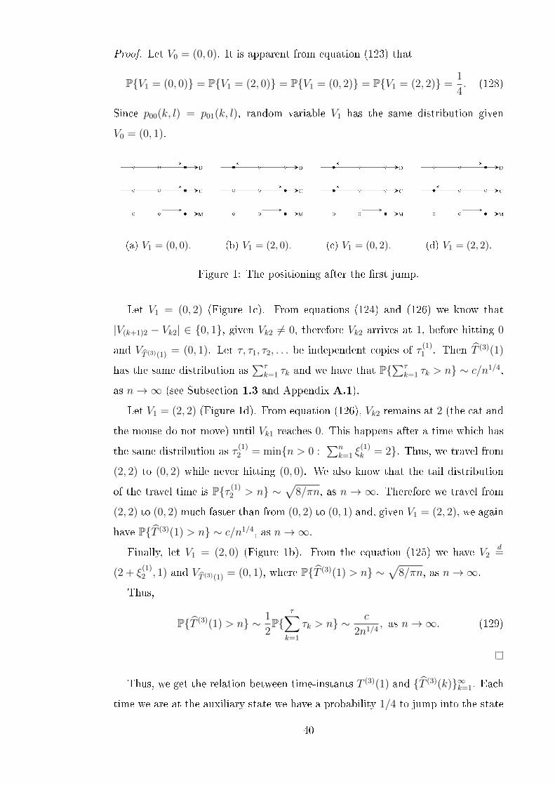
Proof. Let V0 = (0, 0). It is apparent from equation (123) that
P{V1 = (0, 0)} = P{V1 = (2, 0)} = P{V1 = (0, 2)} = P{V1 = (2, 2)} =1
4. (128)
Since p00(k, l) = p01(k, l), random variable V1 has the same distribution given
V0 = (0, 1).
(a) V1 = (0, 0). (b) V1 = (2, 0). (c) V1 = (0, 2). (d) V1 = (2, 2).
Figure 1: The positioning after the �rst jump.
Let V1 = (0, 2) (Figure 1c). From equations (124) and (126) we know that
|V(k+1)2 − Vk2| ∈ {0, 1}, given Vk2 6= 0, therefore Vk2 arrives at 1, before hitting 0
and VT (3)(1) = (0, 1). Let τ, τ1, τ2, . . . be independent copies of τ(1)1 . Then T (3)(1)
has the same distribution as∑τ
k=1 τk and we have that P{∑τ
k=1 τk > n} ∼ c/n1/4,
as n→∞ (see Subsection 1.3 and Appendix A.1).
Let V1 = (2, 2) (Figure 1d). From equation (126), Vk2 remains at 2 (the cat and
the mouse do not move) until Vk1 reaches 0. This happens after a time which has
the same distribution as τ(1)2 = min{n > 0 :
∑nk=1 ξ
(1)k = 2}. Thus, we travel from
(2, 2) to (0, 2) while never hitting (0, 0). We also know that the tail distribution
of the travel time is P{τ (1)2 > n} ∼
√8/πn, as n → ∞. Therefore we travel from
(2, 2) to (0, 2) much faster than from (0, 2) to (0, 1) and, given V1 = (2, 2), we again
have P{T (3)(1) > n} ∼ c/n1/4, as n→∞.
Finally, let V1 = (2, 0) (Figure 1b). From the equation (125) we have V2d=
(2 + ξ(1)2 , 1) and VT (3)(1) = (0, 1), where P{T (3)(1) > n} ∼
√8/πn, as n→∞.
Thus,
P{T (3)(1) > n} ∼ 1
2P{
τ∑k=1
τk > n} ∼ c
2n1/4, as n→∞. (129)
Thus, we get the relation between time-instants T (3)(1) and {T (3)(k)}∞k=1. Each
time we are at the auxiliary state we have a probability 1/4 to jump into the state
40

D(n) = C(n) = M(n) independent of anything else. Using the latter lemma and
the results of Section 1.5 from Borovkov & Borovkov (2008) we get the following
result.
P r o p o s i t i o n 4.2. Let ν = inf{k ≥ 1 : T (3)(k)− T (3)(k − 1) = 1}. Then
ν has a geometric distribution with parameter 1/4 and
P{J (3)1 > n} = P{T (3)(ν) > n} ∼ 4P{T (3)(1) > n}, as n→∞ (130)
and therefore there exists a positive random variable D(3) with a stable distribution
such that
T (3)(n)
n4=
∑nk=1 J
(3)k
n4⇒ D(3), as n→∞. (131)
� 4.4. Distribution of random variable Y(3)
1
In the previous Subsection we analysed the time our process spends between
auxiliary states. In this Subsection we analyse the total jumps of the mouse
between the states (it can have either zero jumps, one jump, or two jumps).
Let {Zk}∞k=0 be an auxiliary Markov chain which satis�es Zk = C(T (3)(k)) −
M(T (3)(k)) ∈ {−1, 0, 1}. Note that Z0 = Zν = 0. Straightforward calculations
show that the transition matrix of our auxiliary Markov chain (state "0" is in the
beginning, then "1" and then "−1") is
PZ =
14
38
38
14
58
18
14
18
58
. (132)
Let
ξ(3)k = M(T (3)(k))−M(T (3)(k − 1)) for k ≥ 1. (133)
Let {ψ1k}∞k=1 be independent copies of τ
(1)1 and let {ψ2
k}∞k=1 be independent copies of∑τ(1)1k=1 ψ
1k. Assume that ζ has binomial distribution with parameter 1/2 independent
of {ψ1k}∞k=1 and {ψ2
k}∞k=1. Then we have
P{ξ(3)2 = ±1, T (3)(2)− T (3)(1) = 1| Z1 = 0, Z2 = 0} =
1
2, (134)
P{ξ(3)2 = 0, T (3)(2)− T (3)(1) = 1| Z1 = ±1, Z2 = 0} = 1, (135)
41

P{ξ(3)2 = m, T (3)(2)− T (3)(1) = k| Z1 = 0, Z2 = ±1}
=
16P{ψ1
2 = k}, if m = ±2 or m = 0,
23P{ζψ1
2 + ψ22 = k}, if m = ±1,
(136)
P{ξ(3)2 = m, T (3)(2)− T (3)(1) = k| Z1 = ±1, Z2 = ±1}
=
15P{ψ1 = k}, if m = ±1,
45P{ζψ1 + ψ2 = k}, if m = 0,
(137)
P{ξ(3)2 = ∓1, T (3)(2)− T (3)(1) = k| Z1 = ±1, Z2 = ∓1} = P{ψ1 = k}. (138)
We have |ξ(3)1 | ≤ 2 and random variable ν has a light-tailed distribution (see
Subsection 1.3). Therefore, random variable Y(3)
1 = M(J(3)1 ) =
∑νk=1 ξ
(3)k has a
light-tailed distribution. Using that and a symmetry argument we get the following
result.
P r o p o s i t i o n 4.3. We have EY (3)1 = 0 and E(Y
(3)1 )m <∞, for any m ≥ 2.
� 4.5. Proof of Theorem 1.21
Random vectors {Y (3)n , J
(3)n }∞n=1 are independent and identically distributed,
where Y(3)
1 =∑ν
k=1 ξ(3)k and J
(3)1 = T (3)(1) = T (3)(ν). We have
η(t) = max{n > 0 :n∑k=1
J(3)k ≤ t} and M(t) =
η(t)∑k=1
Y(3)k . (139)
From Propositions 4.2 and 4.3 we have
EY (3)1 = 0, E(Y
(3)1 )m <∞, for m ≥ 2, and P{J (3)
1 > n} ∼ c
n1/4, (140)
as n→∞. From Theorem 5.1 from Kasahara (1984) (see also Appendix A.2) we
have M(nt)√VarY
(3)1 n1/8
, t ≥ 0
D⇒ {B(E(3)(t)), t ≥ 0}, as n→∞, (141)
where B(t) is a standard Brownian motion, independent of E(3)(t).
42
We show now that (141) holds withM(nt) in the place of M(nt). It is su�cient
to prove that for any �xed T > 0
max1≤k≤[nT ]
{Mk −Mk
}n1/8
a.s.→ 0 as n→∞. (142)
In the time interval (η(nt), nT ] there are no time-instants n when D(n) =
C(n) = M(n), however the mouse may have jumps. Nevertheless, the number of
this jumps can be bounded by 2ν, where the random variable ν has a geometric
distribution with parameter 1/4.
Let Un = maxT (3)(n−1)≤l≤T (3)(n) |Ml −Ml|, n ≥ 1. We have
max1≤l≤J(3)
1
|Ml −Ml|d
≤ν∑k=1
|ξk|. (143)
P r o p o s i t i o n 4.4. For anym ≥ 1 we have EUm1 <∞ and n−1/m max1≤l≤n Ul
converges to 0 a.s., as n→∞.
We have η(nT ) → ∞ a.s. and there exists an random variable ζ such that
n−1/4η(nT )⇒ ζ, as n→∞ (see, e.g., Section XI.5 in Feller (1971b) or Subsection
1.3.3). Thus,
|max1≤k≤[nT ]
{Mk −Mk
}|
n1/8≤
max1≤l≤η(nT ) {Ul}n1/8
+2ν
n1/8
=max1≤l≤η(nT ) {Ul}
η1/4(nT )
(η(nT )
n1/2
)1/4
+2ν
n1/8
a.s.→ 0. (144)
This completes the proof of Theorem 1.21.
43

Part II. Stability of neural networks
SECT ION 5
Introduction and main results
� 5.1. Modelling of neural networks
We analyse the stochastic stability of a model of a neural network. Our model is
inspired by the stochastic integrate-and-�re neuron model. The original model of
membrane potentials was introduced by Lapicque (1907) and has been developed
over the years (for a review of the model see, e.g., Burkitt (2006a,b)). In this
model, at any time t, the internal state of a neuron i is given by its membrane
potential Zi(t), which evolves according to a stochastic di�erential equation
dZi(t) = F (Zi(t), I(t), t)dt+ σ(Zi(t), I(t), t)dWi(t), (145)
where F is a drift function, σ the di�usion coe�cient, I is the neuronal input,
and Wi is a Brownian motion (see, e.g., Gerstner and Kistler (2002)). The process
Wi(t) represents combined internal and external noise. The process I models �rings
of neurons' potentials (or �spikes�): whenever a potential Zi(t) reaches certain
threshold, it resets to a base-level, and the neuron sends signals to other neurons.
A large number of experiments have given us an understanding of the dynamics
of a single neuron. For example, Hodgkin and Huxley (1952) found three di�er-
ent types of ion current �owing through a neuron's membrane, and introduced
a detailed model of a membrane potential. To give a basic description, without
any input, the neuron is at rest, corresponding to a constant membrane potential.
Given a small change, the membrane potential returns to the resting position. If the
membrane potential is given a big enough increase, it reaches a certain threshold,
and exhibits a pulse-like excursion that will a�ect connected neurons. After the
pulse, the membrane potential does not directly return to the resting potential,

but goes below it. This is connected to the fact that a neuron can not have two
spikes one right after another.
A neuron network may be thought of as a connected graph of neurons with
synapses serving as edges between vertices. When a presynaptic neuron �res a
spike it sends a signal through a synapse to a postsynaptic neuron. A neuron is
called inhibitory if its signals predominantly move the membrane potentials away
from a threshold; and excitatory if they predominantly move potentials toward a
threshold. In this paper, we consider a model containing inhibitory neurons only.
It is important to point out that the e�ect of a signal depends on the potential
of a receiving neuron. For example, if the membrane potential of a postsynaptic
neuron is lower than that of a corresponding inhibitory synapse, the e�ect of a
signal will be reversed. Therefore, in the models where signals and potentials are
assumed to be independent, it is important to assume that the potentials should
not decrease too much.
A classical model, introduced by Stein (1965), is the so-called leaky integrate-
and-�re neuron model, where
F (Zi(t), I(t), t) = −αZi(t) + I(t), σ(Zi(t), I(t), t) = σ = const. (146)
There are several variations of this model. For instance, nonlinear models were
considered, such as the quadratic model (see, e.g., Latham et al. (2000)) where
−αZi(t) is replaced with a(Zi(t) − zrest)(Zi(t) − zc), where zc > zrest. Another
direction for generalisation of this model is the Spike Response Model (see, e.g.,
Gerstner and Kistler (2002), Chapter 4.2). In this model, the relation between
the dynamics and the potential is determined by the time of the last spike. This
allows one to explicitly forbid spikes to occur one right after another and to write
the dynamics in integrated form.
5.1.1. Perfect integrate-and-�re neuron model
In the thesis we consider the so-called perfect integrate-and-�re neuron model,
where α = 0 and, therefore, the decay of the membrane potential over time is
neglected. This restriction is a stepping stone to achieve more general results and
it allows us to write the model in integrated form.
45
In our model, the spikes and corresponding signals are represented by shifts
from a threshold of a random length, independent of everything else. We analyse
the system under certain conditions on the distribution of those shifts and prove
stability. Instead of considering the recurrence of sets [−k,H]N (where H is the
threshold and N is the number of neurons), we move each coordinate down and
re�ect the system to work with more convenient sets [0, k + H]N . Thus, in our
model, membrane potentials are nonnegative processes that jump to a random
positive level after reaching zero. Signals from inhibitory neurons push membrane
potentials away from the threshold, i.e. they are positive shifts. It is important to
note that we assume that the travel time of signals between neurons is zero, which in
general can cause uncertainty in the order of spikes. However, the inhibitory signals
do not cause spikes right away, and we assume that the potentials Zi(t) almost
surely do not reach their thresholds at the same time. We refer to Taillefumier et
al. (2012) for a further discussion.
It is often assumed that the studied system of neurons is itself a part of a much
larger system of neurons. The e�ect of the larger system on the sub-system under
consideration is often modelled by a multivariate Brownian motion W (t) with a
drift (the drift guaranties the stability of a system of a single neuron). However,
we can generalise it to a multivariate spectrally positive (i.e. with positive jumps
only) L�evy process X(t) to account for inhibitory signals. It is important for
our analysis that the signals do not in�uence the dynamics of the process Z(t)
if it is away from the threshold, i.e. we have dZ(t) = dX(t) if Zi(t) > 0, for
i ∈ {1, . . . , N}. Nevertheless, the number of spikes ηi(t) before time t is essential
to the stability analysis. The fact that ηi(t) is not pathwise monotone with respect
to signal sizes or the initial state brings certain di�culties in proving stability.
As mentioned above, the system of a single neuron is stable. However, for a
general distribution of signals between neurons, 'partial stability' (see, e.g., Cottrell
(1992) and Fricker et al. (1994)) can occur when only a (possibly random) subset
of neurons stabilises, while membrane potentials of other neurons are �pushed� to
in�nity (which contradicts the physical setup). This situation is of independent
mathematical interest and there is no detailed discussion in the Thesis.
It is possible to analyse this model similarly to queueing networks (see, e.g.,
Asmussen and Turova (1998) and references therein). For example, instead of
46
membrane potentials one may consider residual times (R1(t), . . . , RN(t)) until a
spike. In other words, Ri(t) is the time that the process (Xi(t+ s)−Xi(t), s ≥ 0)
needs to reach −Zi(t). Thus, we have N queues with workloads decreasing at unit
speed. When one of the residual times Ri(t−) becomes zero this triggers a spike,
and, potentially, every queue (depends on the connectivity of the system) has an
arrival of additional workload. More precisely, assume that Ri(t−) = 0 and let ξij
represent the signals, produced by the spike. Then every residual time Rj(t−) is
increased by θij which is the time that the process
(Xj(t+Rj(t−) + s)−Xj(t+Rj(t−)), s ≥ 0) (147)
needs to reach −ξij. It is very signi�cant that the arrivals of workloads are syn-
chronised, and it brings interesting consequences for the analysis.
� 5.2. General overview of our results
The ideas and methods for stability analysis of stochastic systems and networks
using scaling limits that are linear both in space and in time have become popu-
lar and have been developed in 80's�90's of the last century, thanks to works by
V.A. Malyshev and his co-authors (see Malyshev (1972), Malyshev and Menshikov
(1979), Ignatyuk and Malyshev (1991), and Malyshev (1993)) where the so-called
second vector �led has been introduced, and later works by A.N. Rybko, A.L. Stol-
yar and J. Dai (see Rybko and Stolyar (1992), Dai (1995), and Stolyar (1995)) who
introduced �uid limits. In our analysis of neural networks, we follow the latter ap-
proach. Although this method is usually applied to queueing networks, it is quite
universal, and turns out to also be applicable to our model. We also refer to Foss
and Konstantopoulos (2004) for an overview of some stochastic stability methods.
In particular, we introduce �uid limits and prove their piecewise linearity under
speci�c conditions on average signals and the drift EX(1). Then we study con-
vergence of the �uid limits to zero and apply (a version of) the stability criterion
introduced by Dai (1995) that says that stability of all �uid limits implies positive
recurrence of the underlying Markov process. We then prove the existence of a
so-called minorant measure. Thus, we can use results from Section 7 of Borovkov
and Foss (1992) (see, also, Chapter VII of Asmussen (2003)) to prove convergence
to the stationary distribution in total variation.
47

5.2.1. Fluid model and positive recurrence
Let us start with an example of multiclass queueing network. Let {1, . . . , K} be
a set of customer classes and {1, . . . , J} a set of stations. Each station j is a single-
server service facility that serves customers from the set of classes c(j) according
to a non-idling, work-conserving, non-preemptive, but otherwise general, service
discipline. It is assumed that c(j)∩c(i) = 0 if i 6= j. There is a single arrival stream
A(t) of intensity λ. The service for customers from class k goes with intensity µk.
Routing at the arrival point is done according to probabilities pk, so that an arriving
customer becomes of class k with probability pk. Routing in the network is done so
that a customer �nishing service from class k joins class l with probability pk,l. Let
Ak(t) be the cumulative arrival process of class k customers from the outside world.
Let Dk(t) be the cumulative departure process from class k. The process Dk(t)
counts the total number of departures from class k, both those that are recycled
within the network and those who leave it. Of course, it is the speci�c service
policies that will determine Dk(t) for all k. If we introduce independent identically
distributed routing variables {αk(n), n ∈ Z+} so that P{αk(n) = l} = pk,l, then we
may write the class-k dynamics as:
Qk(t) = Qk(0) + Ak(t) +K∑l=1
Dl(t)∑n=1
I(αl(n) = k)−Dk(t). (148)
There are various other equations satis�ed by the queueing system, which we omit.
Now, denote the sum of all initial conditions (initial workload, the time until the
�rst arrival and remaining service times) as N . While it is clear that Ak(Nt)/N
has a limit as N → ∞, it is not clear at all that so do Dk(Nt)/N . The latter
depends on the service policies, and, even if a limit exists, it may exist only along
a certain subsequence. We say that X(·) is a limit point of XN(·) if there exists
a deterministic subsequence {Nl}, such that, XNl → X, as l → ∞, almost surely
and uniformly on every compact set. Denote D(t) = (D1(t), . . . , DK(t)). A �uid
limit is any limit point of the sequence of functions {D(Nt)/N, t ≥ 0} and the �uid
model is the set of these limit points. If D(t) = (D1(t), . . . , DK(t)) is a �uid limit,
then we can de�ne
Qk(t) = Qk(0) + Ak(t) +K∑l=1
Dl(t)pl,k −Dk(t), for k = 1, . . . , K. (149)
48

It can be interpreted the following way: since D(Nt)/t→ D(t), along, possibly, a
subsequence, then, along the same subsequence, Q(Nt)/N → Q(t). This follows
from the FLLN for the arrival process and for the switching process.
We say that the �uid model is stable, if there exists a deterministic t0 > 0, such
that, for all �uid limits, Q(t) = 0 for t ≥ t0 , almost surely. Equivalently the �uid
model is stable if there exist a deterministic time t0 > 0 and a number ε ∈ (0, 1)
such that, for all �uid limits, Q(t0) ≤ 1− ε, almost surely.
P r o p o s i t i o n 5.1. Denote the state of the system at the arrival epochs as
{Xn}∞n=1. If the �uid model is stable, then there exists a bounded set B which is
positive recurrent for {Xn}∞n=1.
The latter is proven via Lyapunov function criterion (see Foss and Konstanto-
poulos (2004)).
The de�nition of stability of a �uid model is quite a strong one. Nevertheless,
if it holds - and it does in many important examples - then the original multiclass
network is stable. However, in a case of random �uid limits one might consider
alternative weaker versions.
In the thesis we take Markov process Zz(t) with Zz(0) = z ∈ R+N . Let ‖z‖ =∑Ni=1 zi for z ∈ R+N . We introduce a family of scaled processes
Zz =
{Zz(t) =
Zz(‖z‖t)‖z‖
, t ≥ 0
}. (150)
We then analyse the convergence of such processes as ‖z‖ → ∞. We prove that
the �uid limits are piecewise deterministic and linear. Next, we prove stability of
all �uid limits, which implies existence of a bounded positive recurrent set. Now,
in the example we consider a Markov chain constructed on the arrival epochs.
Following the lines of Dai (1995) one can get the result for continuous time. Thus,
we prove the existence of a bounded set V such that
τ z(ε, V ) = inf{t ≥ ε : Zz(t) ∈ V } <∞ almost surely and supz∈V
Eτ z(ε, V ) <∞.
(151)
5.2.2. Ergodicity of processes admitting embedded Markov chains
We discussed positive recurrence for Markov processes. Now we move to ergodi-
city or convergence to stationary distribution. For reference see, e.g., Borovkov
49
and Foss (1992). Let (X,BX) be an arbitrary measurable space and let X =
(X(x, n))∞n=0 be an X-valued Markov chain with the initial state X(x, 0) = x ∈ X.
Assume that there exist a positive recurrent set V , a probability measure ϕ on
(X,BX), a number p ∈ (0, 1), and a non-negative integer m ≥ 0 such that
infx∈V
P{X(x,m+ 1) ∈ B} ≥ pϕ(B) for any B ∈ BX. (152)
DenoteX(ϕ, n) as a Markov chain with a random initial value distributed according
to ϕ. Let τV (ϕ) = inf{n ≥ 1 : X(ϕ, n) ∈ V }. Let k1, k2, . . . be the integer numbers
for which P{τV (ϕ) = ki} > 0. Assume that there exists a number l > 0 such that
the greatest common divisor of the set (m+ k1 + 1,m+ k2 + 1, . . . ,m+ kl + 1) is
equal to one (this condition is satis�ed ifm = 0 and ϕ(V ) > 0). Then the following
proposition holds.
P r o p o s i t i o n 5.2. (Theorem 2.1, Borovkov and Foss (1992)) There exists
a stationary Markov chain (Xn)∞n=0 with transition probability P(x,B) de�ned on
the same probability space with X, which independent of X(0) and such that for
each x ∈ X
P{X(x, k) = Xk for all k ≥ n} → 1, as n→∞. (153)
Relation (153) implies necessarily that the distribution π(B) = P{X0 ∈ B} of
X0 is an invariant measure:
π(B) =
∫X
π(dx)P(x,B), B ∈ BX, (154)
and the convergence in total variation occurs
supB∈BX
|P{X(x, n) ∈ B} − π(B)| → 0, as n→∞. (155)
Such results for Markov chains can help in the analysis of special stochastic
processes. Take a stochastic process {Z(t), t ≥ 0}. Denote a sequence of embedded
times (Tn)∞n=0 such that T0 ≥ 0 and (en)∞n=0 = (Tn+1 − Tn)∞n=0 are positive random
variables. Denote σ-algebra F(t) = σ{Z(u); u ≤ t}.
D e f i n i t i o n 5.3. Process Z admits an embedded Markov chain if there exists
a sequence of Markov times (Tn)∞n=0 such that
• the sequence X(n) = Z(Tn) constitutes a homogeneous Markov chain;
50

• for any n ≥ 0, t ≥ 0 the joint distribution of {Z(Tn + t), (en+k)∞k=0} depends
on Z(Tn) = X(n) and t only, i.e.,
P{Z(Tn + t) ∈ B, (en+k)∞k=0 ∈ D| F(Tn)} (156)
= P{Z(Tn + t) ∈ B, (en+k)∞k=0 ∈ D| σ(X(n))}
almost surely for any B ∈ BX and D ∈ BR∞+.
Assume that X(n) follows the same conditions as before (positive recurrent set,
minorant measure and aperiodicity). For embedded times we assume
supx∈X
E (e0| X(0) = x) <∞. (157)
Denote by τ(y) a random variable with the distribution
P{τ(y) > t} = P{Tµ − T0 > t| X(0) ∈ dy}, (158)
where µ is the �rst hitting time of the set V by X(n) and ϕ is the minorant
measure.
P r o p o s i t i o n 5.4. (Theorem 7.3, Borovkov and Foss (1992)) Assume that
process {Z(t), t ≥ 0} satis�es the following:
1. the distribution
P{τ > t} =
∫ϕ(dy)P{τ(y) > t} (159)
of the random variable τ is a non-lattice one;
2. the trajectories of the process Z are right (or left) continuous.
Then the distributions Pt(·) = P{Z(t) ∈ ·} weakly converge to some probability
distribution. If instead of the �rst condition we require the distribution of τ to pos-
sess an absolutely continuous component, the second condition becomes redundant
and the convergence is in total variation.
Thus, to prove convergence in total variation we �nd a proper embedding (we
assume that (en)∞n=0 are independent uniformly distributed bewteen one and two)
with absolutely continuous component. Through �uid approximation model we
prove positive recurrence. Finally, we prove that Lebesgue measure on a bounded
set is a minorant measure for embedded Markov chain.
51

5.2.3. Related results
Let us return to the residual-time model (R1(t), . . . , RN(t)). There is a series
of papers studying ergodic properties of such models. Assume that θij = θ(i) for
j 6= i. Cottrell (1992) study conditions for the model to be ergodic when 'residual
times' θii are exponential and θ(i) are constants. Fricker et al. (1994) maintained
the exponential assumption for θii but allowed θ(i) to have a general distribution.
The authors give broad stability analysis for several types of networks. For the
embedded Markov chain Rn, which takes the values of R(t) right after the spikes,
the authors acquire an explicit form of the stationary distribution. The result
involves the stationary waiting times of N separate M/G/1 queues, with inter-
arrival times and service times for the i-th queue having the same distribution as
θii and θ(i) respectively, and it is proved via Laplace transforms. Karpelevich et
al. (1995) consider a more general architecture of the connections in the network
and give necessary and su�cient conditions for ergodicity. Asmussen and Turova
(1998) get rid of the exponential assumption on θii via a sample path approach
which highlights the connection to other applied probability areas such as renewal
theory, queueing theory and point processes. This approach allows the authors to
generalise the result of Fricker et al. (1994) for Rn, and it provides the key for
studying further aspects of the neural model.
Next, we go back to the membrane potentials. The stochastic integrate-and-
�re neuron model has received an increasing amount of attention in recent years.
There are a number of papers considering mean-�eld limits of such systems, i.e.,
letting the number of neuronsN becomes large while assuming interactions of order
1/N . The resulting nonstandard equations of McKean�Vlasov-type is the subject
of C�aceres et al. (2011) from a PDE perspective and Delarue et al. (2015) from a
stochastic point of view. The introduction of excitatory neurons may lead to a very
interesting behaviour in the limit. Namely, these works show that, even though
for a certain choice of parameters the limit equation has a unique global-in-time
solution, nevertheless, there is a choice of parameters which leads to a blow-up
phenomenon in �nite time. In other words, the e�ect of a single neuron spiking
may cause an instantaneous cascade during which a signi�cant portion of neurons
has a spike. This brings challenges for the approximation of the �nite system by
52

the limiting one after a blow-up.
It is important to mention that in the thesis we consider a relatively simple
model as a cornerstone for future research (including mean-�eld limits and intro-
duction of excitatory neurons). Nevertheless, there is a vast variety of advanced
models for which signi�cant results are obtained. Next, we introduce several ex-
amples of works dealing with such models.
De Masi et al. (2015) consider a special case of N identical inhibitory neurons
with N → ∞. Firstly, the evolution of membrane potentials is deterministic
between spikes. Secondly, each membrane potential has a drift to the average
potential. Finally, spikes do not occur at the moments when a potential reaches
a certain threshold. Instead, there is a spiking rate of the system which depends
on the current membrane potentials. The spiking neuron returns to the resting
potential and sends signals of size 1/N to every other neuron. The authors regard
the state of the neurons UN(t) = (UN1 (t), . . . , UN
N (t)) as a distribution of 1/N valued
Dirac masses placed at the positions UN1 (t), . . . , UN
N (t). As N goes to in�nity, the
authors study the limiting fraction of neurons with potentials belonging to a certain
interval and introduce non-linear PDE which describes it. The usual approach to
prove hydrodynamic limits in mean-�eld systems is to show that propagation of
chaos holds. However, the potentials are correlated due to instantaneous signals
through the whole system. To get the result the authors use coupling methods on
a discrete-time version of the process.
Robert and Touboul (2016) also consider a model without a �xed spiking
threshold. The authors consider a system of N excitatory neurons. Here spikes
occur as a inhomogeneous Poisson process and spiking rate is, again, a function
of a current membrane potential. The signals between neurons ξ(n)ij are independ-
ent identically distributed random variables. The main di�erence is the leaking of
membrane potentials: without interactions between neurons a potential behaves
according to dZi(t) = −Zi(t)dt. The authors analyse invariant distributions for
�nite-sized networks and then for the averaged limit. For the �nite case the au-
thors prove that, in the presence of an external noise (spiking rate at 0 is positive),
there exists a unique non-trivial invariant distribution for the system, and the sys-
tem �dies out� (no spikes occur after some time) if the spiking rate at 0 is zero.
Additionally, the authors prove Harris positive recurrence using a regeneration ar-
53

gument. For the in�nite case the authors prove that, under some growth conditions
on the spiking rate and other technical conditions, a mean-�eld result holds. It is
important to mention that discontinuities produced by Poisson processes bring a
big challenge for the analysis of this model.
Inglis and Talay (2015) also consider a system of excitatory neurons. However,
the authors modify the model in order to deal with the aforementioned blow-
up phenomenon. More precisely, the signals are constant, however, instead of
instantaneous transmission between neurons the in�uence of a spike is described
by a cable equation: if a neuron i spikes at time s then the total impact from
that spike on neuron j at time t > s is Jij∫ tsG(t − s)ds. The authors investigate
convergence of the averaged system, and they prove the existence and uniqueness
of solution for the limiting system.
� 5.3. Structure of Part II
This part of the Thesis is structured as follows. In Subsection 5.4 we de�ne
our model, introduce auxiliary concepts and notations, and formulate our results.
In Section 6 we prove Theorem 5.6. In particular, in Subsection 6.1 we introduce
the �uid model and formulate related technical results. In Subsection 6.2 we prove
important auxiliary results. In Subsection 6.4 we discuss possible generalisations
of our results. In Subsection 6.3 we prove positive recurrence. In Subsection 6.5
we prove that our model satis�es the classical �minorization� condition. In Section
7 we consider two simple examples of our model, show possible characteristics
we want to acquire in general setting, and introduce another direction for future
research. Section 8 is an illustration of various directions for the future research.
Appendix B includes the remaining auxiliary results and comments.
� 5.4. Model and results
We analyse a network of N stochastic perfect integrate-and-�re inhibitory neur-
ons. At any time t, the internal state of all neurons is given by a multidimensional
process Z(t) which represents neurons' membrane potential. Let X(t) be a N -
dimensional spectrally positive left-continuous L�evy process with a �nite mean,
and assume that its distribution has a non-degenerate absolute continuous com-
54

ponent. The process X(t) represents combined internal and external noise. Let
µi = −EXi(1) > 0 and X0i (t) = µit + Xi(t). While Z(t) ∈ (0,∞)N , membrane
potentials evolve as the process X(t), i.e. dZ(t) = dX(t). However, if one of
the coordinates becomes non-positive, a shift of independent size occurs for all
the coordinates. Let us describe this shift. Let {{ξ(k)ij }Ni,j=1}∞k=1 be i.i.d. random
matrices, independent of everything else, with a.s. strictly positive elements. Let
bij = Eξ(1)ij <∞ and Sij(n) =
∑nk=1 ξ
(k)ij , for i, j ∈ {1, 2, . . . , N}. If potential Zi(t)
hits non-positive values for the k-th time, then instantaneously it increases to ξ(k)ii
and other membrane potentials increase by ξ(k)ij . We call this event �a spike of
neuron i�.
Thus, we can see the process Z(t) as a 're�ected version' of the process X(t):
whenever the trajectory hits the border it bounces away. However, when one
coordinate �bounces away� all other coordinates are pushed as well. Therefore, we
can say that each surface zi = 0 is assigned to a vector (bi1, bi2, . . . , biN) which
describes an average change of trajectory upon hitting the surface. Such analogy
works only because we restrict the trajectories ofX(t) to not have jumps downward
and signals ξ(k)ij are positive. Thus, the trajectory can not jump over the border
and the shift given by a spike is independent of the past.
R ema r k 5.5. One can allow the absolute continuous component of the distri-
bution of the process Xi(t) to be degenerate (for example, take a sum of a Poisson
process and a linear function −at) and, instead, assume the distribution of the
matrix {ξ(1)ij }Ni,j=1 to have an absolute continuous component. The main result of
this part would still hold and the proof would only need few minor changes.
Let Zz(t) = (Zz1 (t), . . . , ZzN(t)) ∈ Z = [0,∞)N be the membrane potentials at
time t with an initial value z = (z1, . . . , zN). Let T zi0 = 0 and let
T zik = inf{t > T zi(k−1) : Zzi (t) ≤ 0}, for k ≥ 1, (160)
be the times when neuron i reaches its threshold. Let ηzi (0) = 0 and let ηzi (t) =
max{k : T zik < t} be the number of spikes of Zzi (t) before time t. Then the
dynamics of the system is given by
Zzi (t) = zi+Xi(t)+N∑j=1
ηzj (t)∑k=1
ξ(k)ji = zi+Xi(t)+
N∑j=1
Sji(ηz
j (t)), i = 1, . . . , N. (161)
55

Before talking about stability of the system it is important to point out that,
due to the negative drift, one can easily show that the potential of an isolated
neuron is stable (this is also a subcase of our main result). Nevertheless, there are
examples of parameters µi and bij such that there exists a subset of neurons which,
after reaching stability, can �push other neurons to in�nity�. We do not give any
details on such cases of partial stability in the thesis. Next, we introduce some
simple assumptions which allow to avoid partial stability and prove an ergodic
result. However, these conditions are far from necessary for stability and they
serve as a nice example where resulting characteristics have a clear and explicit
form. We provide a discussion of possible necessary and su�cient conditions in
Subsection 6.4.
We assume that all potentials have the same drift µ and that signals from
neuron i = 1, . . . , N to all other neurons have the same mean wi. More precisely,
we assume that
µi = µ > 0, bij = Eξ(1)ij = wi > 0 and bii = Hi > wi, for i = 1, . . . , N and j 6= i.
(162)
However, we allow the distributions of potentials and of signals to di�er.
Th e o r em 5.6. Assume condition (162) to hold. Then the process
(Zz
1(t), . . . , Zz
N(t)) is Harris positive recurrent: there is a distribution π such that
supA|P{Zz(t) ∈ A} − π(A)| → 0, as t→∞. (163)
R ema r k 5.7. Given (162), matrix B = (bij)Ni,j=1 is invertible and
(1B−1)i =1
(Hi − wi)(
1 +∑N
k=1wk
Hk−wk
) , for i = 1, . . . , N , (164)
where 1 = (1, . . . , 1). Vector µ1B−1 represents rates of spikes when stability is
achieved. In particular, for large t > µ−1(1 +∑N
k=1wk/(Hk − wk)) and for each
sequence zn, ‖zn‖ → ∞, there exists a subsequence znk such that
ηznk (‖znk‖(t+ ∆))− ηznk (‖znk‖t)‖znk‖∆
⇒ µ1B−1, for ∆ > 0. (165)
Here we use vector-norm ‖x‖ =∑N
i=1 |xi|.
We prove Theorem 5.6 following two standard steps. For the reader's conveni-
ence, we formulate those steps as lemmas. Let τ z(ε, B) = inf{t > ε : Zz(t) ∈ B}
56

be the �rst hitting time of a set B after time ε. The �rst step is the proof of
positive recurrence which we achieve via the �uid approximation method.
L emma 5.8. There exists k0 > 0 such that for V = {z ∈ Z : ‖z‖ < k0} we
have
supz∈V
Eτ z(ε, V ) <∞. (166)
In the second step, we show that our model satis�es the classical 'minorization'
condition.
L emma 5.9. There exist a number p > 0 and a probability measure ψ,
such that for a uniformly distributed random variable U ∈ [1, 2], independent of
everything else, we have
infz∈V
P{Zz(U) ∈ B} ≥ pψ(B). (167)
Using Lemmas 5.8 and 5.9 we can prove that conditions of Theorem 7.3 from
Borovkov and Foss (1992) (see also Subsection 5.2.2) are satis�ed, which implies
Harris positive recurrence. More precisely, let (Tn)∞n=0 be a sequence of embedded
times. Let (en)∞n=0 = (Tn+1 − Tn)∞n=0 are independent random variables uniformly
distributed between one and two. Then the Markov chain (Z(Tn))∞n=0 is Harris
positive recurrent. Additionally, measure ψ and the distribution of e0 follow cer-
tain 'spread out property', meaning, they have an absolute continuous component.
Thus, we have �enough mixing� in continuous time and process (Z(t), t ≥ 0) is
Harris positive recurrent as well.
The proof of Lemma 5.8 is based on the �uid approximation. We dedicate
Subsection 6.1 formulating corresponding de�nitions and auxiliary results. We
point out that we need to assume condition (162) only in the proof of Lemma 5.8
and in Remark 5.7.
One of the di�culties of our model is the lack of path-wise monotonicity for the
number of spikes ηz(t) with respect to signals ξ(k)ij or initial state z. In general,
making one neuron �ring a spike earlier may lead to other spikes occurring later.
However, we prove that there is a �partial monotonicity� which allows us to get an
upper bound for process ηz(t) with useful properties.
Since all neurons are inhibitory, one way to increase the number of spikes is to
remove all interactions between neurons. Let the process Zz be the transformation
57

of the process Zz by replacing signals ξ(k)ji , j 6= i, by 0 for k ≥ 1 (trajectories of
X(t) remain the same). The resulting process has a simpler dependence between
coordinates and it has a greater number of spikes before any time t > 0 than that
of Zz. For our convenience, we want to remove the dependence of the upper bound
on z (which is signi�cant because we take z large in the following lemmas) and
make the time until the �rst spike to have the same distribution with the rest of
waiting times. Let the process Z be the transformation of the process Zz, so that
Zi(0)d= ξ
(1)ii , 1 ≤ i ≤ N . Let ηz and η be the number of spikes in processes Zz and
Z, respectively.
L emma 5.10. We have
ηzi (t) ≤ ηzi (t), a.s., (168)
ηzi (t)st.
≤ 1 + ηi(t), (169)
and ηi(t) is an undelayed renewal process, which satis�es the integral renewal the-
orem and the SLLN
Eηi(t)t→ µi
bii
a.s.← ηi(t)
t(170)
In the next Section, we present a stability analysis of a class of neural networks
with a general L�evy input. Then, in Section 7, we present two particular examples
of the model, with constant input and with Poisson input, where we can �nd exact
expressions for a number of characteristics.
58

SECT ION 6
Stability of the system with L�evy input
In this Section we introduce the �uid model, prove necessary auxiliary results
and, �nally, give a proof of Theorem 5.6 divided into two parts. We also make
some brief comments on more general conditions for stability of the system in
Subsection 6.4.
� 6.1. Fluid model and corresponding auxiliary results
Let us de�ne the �uid approximation model. Let ρ(x,y) =∑N
i=1 |xi − yi| be
the metric on Z and let ‖x‖ = ρ(x, 0), for x,y ∈ Z. For each z ∈ Z, introduce a
family of scaled processes
Zz =
{Zz(t) =
Zz(‖z‖t)‖z‖
, t ≥ 0
}. (171)
We call the family
Z = {Zz, ‖z‖ ≥ 1} (172)
relatively compact (at in�nity) if, for each sequence Zzn , ‖zn‖ → ∞, there exists a
subsequence Zznk that converges weakly (in the Skorokhod topology) to some limit
process ϕZ = {ϕZ(t), t ≥ 0}, which is called a �uid limit. A family of such limits
is called a �uid model. The �uid model is stable if there exists a �nite constant
T such that ‖ϕZ(T )‖ = 0 a.s. for any �uid limit ϕZ (there are several equivalent
de�nitions of stability of a �uid model, see e.g. Stolyar (1995)). Based on stability
of a �uid model, one can prove positive recurrence of the original Markov process
following the lines of Dai (1995).
Using Lemma 5.10 we prove the next result.
L emma 6.1. The family of processes {Zz, z ∈ Z} is such that
• for all t > 0 and z ∈ Z,
E‖Zz(t)‖ <∞ (173)

and moreover, for any K,
sup‖z‖≤K
E‖Zz(t)‖ <∞; (174)
• for all 0 ≤ u < t, the family of random variables
{ρ(Zz(u), Zz(t)), ‖z‖ ≥ 1} (175)
is uniformly integrable and there exists a constant C such that
lim sup‖z‖→∞
P{ supu′,t′∈[u,t]
ρ(Zz(u′), Zz(t′)) > C(t− u)} = 0. (176)
With this result, one can follow the lines of the proof of Theorem 7.1 from
Stolyar (1995) to obtain the following.
Co r o l l a r y 6.2. The family of processes Z is relatively compact and every
�uid limit ϕZ is an a.s. Lipschitz continuous function with Lipschitz constant
C + 1.
We know that a Lipschitz continuous function is di�erentiable. We call time t0
a regular point if ϕZ(t) is di�erentiable at t0. Furthermore, we have
ϕZ(t)− ϕZ(s) =
∫ t
s
dϕZ
du(u)du, t > s > 0, (177)
where the derivative is arbitrarily de�ned (for example, it equals zero) outside
regular points.
Let ηz(t) = ηz(‖z‖t)/‖z‖. Following the lines of the proof of Lemma 6.1, one
can prove similar results for the family η = {ηz, ‖z‖ ≥ 1}. Denote a �uid limit of
η as ϕη. If at time t we have ϕηi (t) > 0, then for a certain sequence zn the number
of spikes ηzni (‖zn‖t) becomes large. If additionally, ηzni (‖zn‖t) converges to in�nity
a.s., then by the law of large numbers
Sij(ηzni (‖zn‖t))‖zn‖
=ηzni (‖zn‖t)‖zn‖
Sij(ηzni (‖zn‖t))
ηzni (‖zn‖t)⇒ ϕηi (t)bij, as n→∞. (178)
If ϕηi (t) = 0, then the number of spikes is not as large and, if we prove that the
left-hand side of the last equation converges to zero, the resulting convergence will
be of the same form.
Using this idea we get the following result.
60

L emma 6.3. Let ηzn converge weakly to a �uid limit ϕη for a sequence zn,
‖zn‖ → ∞ as n→∞. Then we have weak convergence of processes( 1
‖zn‖
N∑i=1
Sij(ηzni (‖zn‖t))
)N
j=1
, t ≥ 0
D⇒ (ϕη(t)B, t ≥ 0). (179)
� 6.2. Proofs of auxiliary results
In this Subsection we prove our auxiliary results for a general matrix B and
parameters µi.
6.2.1 Proof of Lemma 5.10
We prove that T zik ≥ T zik:
T zik = inf{t > T zi(k−1) : Zzi (t) ≤ 0} = inf{t > T zi(k−1) : Zzi (t) = 0}
= inf{t > T zi(k−1) : zi +Xi(t) +N∑j=1
Sji(ηz
j (t)) = 0}
= inf{t > T zi(k−1) : zi +Xi(t) + Sii(k − 1) +∑j 6=i
Sji(ηz
j (t)) = 0}
≥ inf{t > T zi(k−1) : zi +Xi(t) + Sii(k − 1) = 0}. (180)
Since T zi0 = T zi0 = 0, by induction we have
T zik ≥ inf{t > T zi(k−1) : zi +Xi(t) + Sii(k − 1) = 0} = T zik. (181)
Thus, we get ηzi (t) ≤ ηzi (t). Since ηz
i (t)−1 has the same distribution as ηi(t−T zi1) ≤
ηi(t), we have the second inequality.
The process ηi(t) is an undelayed renewal process with waiting times having the
same distribution as τi = inf{t > 0 : Xi(t) = −ξ(1)ii }. Using the strong law of large
numbers, one can prove that Eτi = bii/µi (see also Borovkov (1965) for a detailed
proof). Therefore, via the standard argument of renewal theory the rest of the
proof follows (see e.g. Feller (1971)).
6.2.2 Proof of Lemma 6.1
Part 1. Using Lemma 5.10 and positivity of ξ(k)ij , we get
‖Zz(t)‖ =N∑i=1
|zi +Xi(t) +N∑j=1
Sji(ηz
j (t))| ≤ ‖z‖+ ‖X(t)‖+N∑i=1
N∑j=1
Sji(ηz
j (t)).
(182)
61

We have
{ηzi (t) = m} = {−m∑k=1
ξ(k)ii < zi + inf
0≤s≤tX(s) ≤ −
m−1∑k=1
ξ(k)ii } (183)
and, therefore,
ηzi (t) = inf{m ∈ Z+ :m∑k=1
ξ(k)ii > −zi − inf
0≤s≤tX(s)}. (184)
Since {{ξ(k)ij }Ni,j=1}∞k=1 and (X(t), t ≥ 0) are independent, the random variable ηzi (t)
is a stopping time for the sequence {{ξ(k)ij }Ni,j=1}∞k=1. By Wald's identity,
ESji(ηzj (t)) = Eηzj (t)∑k=1
ξ(k)ji = Eηzj (t)bji <∞. (185)
Part 2. We have
ρ(Zz(u), Zz(t)) =N∑i=1
|Zzi (‖z‖t)− Zzi (‖z‖u)|‖z‖
≤ (t− u)N∑i=1
µi
+N∑i=1
|X0i (‖z‖t)−X0
i (‖z‖u)|‖z‖
+N∑i=1
N∑j=1
Sji(ηz
j (‖z‖t))− Sji(ηzj (‖z‖u))
‖z‖. (186)
Process Xi is a L�evy process, from which we have
E|X0
i (‖z‖t)|‖z‖
≤ 2 sup0≤s≤t
E|X0i (s)|, for ‖z‖ ≥ 1, (187)
and, therefore, the second summand on the right-hand side of (186) is uniformly
integrable. By Lemma 5.10, we have
Sij(ηz
j (‖z‖t))− Sij(ηzj (‖z‖u))st.
≤ Sij(1 + ηi(‖z‖(t− u))). (188)
Since Sij(n)/n→ bij and ηi(‖z‖(t− u))→∞ a.s., we have
Sij(1 + ηi(‖z‖(t− u)))
1 + ηi(‖z‖(t− u))
a.s.→ bij, (189)
and therefore
0 ≤Sji(η
z
j (‖z‖t))− Sji(ηzj (‖z‖u))
‖z‖st.
≤ Sij(1 + ηi(‖z‖(t− u)))
‖z‖
=1 + ηi(‖z‖(t− u))
‖z‖Sij(1 + ηi(‖z‖(t− u)))
1 + ηi(‖z‖(t− u))→ (t− u)
µibiibij (190)
a.s. and in L1, as ‖z‖ → ∞. Then the distance on the left-hand side of (186) is
bounded above by the sum of uniformly integrable random variables and therefore
is also uniformly integrable.
62
Given
C >N∑i=1
µi
(1 +
N∑j=1
bijbii
), (191)
there exists ε > 0 such that for ‖z‖ large
P{ supu′,t′∈[u,t]
ρ(Zz(u′), Zz(t′)) > C(t− u)}
≤ P
{sup
u′,t′∈[u,t]
N∑i=1
|X0i (‖z‖t′)−X0
i (‖z‖u′)|‖z‖
> ε(t− u)
}
≤ 2NP
{sup
s∈[0,t−u]
|X01 (‖z‖s)|‖z‖
>ε
2N(t− u)
}→ 0, (192)
by Theorem 36.8 from Sato (1999).
6.2.3 Proof of Lemma 6.3
By Skorokhod (1956) (see also Subsection 1.5), it is su�cient to prove that there is
a convergence of �nite-dimensional distributions on everywhere dense set of times
t and that a tightness condition holds. Tightness can be deduced from the second
statement of Lemma 6.1. We prove that
P
{K⋂k=1
N⋂i,j=1
{Sij(η
zni (‖zn‖tk))‖zn‖
< ykij
}}→ P
{K⋂k=1
N⋂i=1
{ϕηi (tk) < min
1≤j≤N
ykijbij
}}(193)
as n→∞, for appropriate t ≥ 0 and y ∈ (0,∞)KN2.
De�ne sets
Ckij(n) =
{Sij(η
zni (‖zn‖tk))‖zn‖
< ykij
}, (194)
Dki (n,m) = {ηzni (‖zn‖tk) > m}, (195)
Ekij(n, δ) =
{∣∣∣∣Sij(ηzni (‖zn‖tk))ηzni (‖zn‖tk)
− bij∣∣∣∣ ≤ δ
}, (196)
F k±i (n, δ) =
{ηzni (‖zn‖tk)‖zn‖
< min1≤j≤N
ykijbij ∓ δ
}, (197)
where δ ∈ (0,mini,j bij). We prove that
P{F k−i (n, δ)
}+ o(1) ≤ P
{N⋂j=1
Ckij(n)
}≤ P
{F k+i (n, δ)
}+ o(1), as n→∞.
(198)
63

For any y ∈ (R+)KN2such that (minj(y
kij/bij))
Ni=1 is a continuity point of the cdf
of (ϕη(tk))kk=1, there is a neighbourhood ∆ of y such that every point x ∈ ∆ is also
a continuity point. Thus, for δ small we have
P
{K⋂k=1
N⋂i=1
F k±i (n, δ)
}= P
{K⋂k=1
N⋂i=1
{ηzni (‖zn‖tk)‖zn‖
< min1≤j≤N
ykijbij ∓ δ
}}
→ P
{K⋂k=1
N⋂i=1
{ϕηi (tk) < min
1≤j≤N
ykijbij ∓ δ
}}, as n→∞,
(199)
and, therefore, by letting δ converge to 0, we get (193).
By the law of large numbers, we have
P{Dki (n,m) ∩ Ek
ij(n, δ)} → 0, as m→∞, (200)
and
P{Ckij(n) ∩Dk
i (n,m)} → 0, as n→∞, (201)
if m = o(‖zn‖). Take m =√‖zn‖.
From the de�nitions we have(N⋂j=1
Ckij(n) ∩Dk
i (n,m) ∩ Ekij(n, δ)
)⊆(F k+i (n, δ) ∩Dk
i (n,m) ∩ Ekij(n, δ)
)=(F k+i (n, δ) ∩Dk
i (n,m))\(F k+i (n, δ) ∩Dk
i (n,m) ∩ Ekij(n, δ)
)(202)
and
(F k+i (n, δ) ∩Dk
i (n,m))
= F k+i (n, δ) \
(F k+i (n, δ) ∩Dk
i (n,m)). (203)
Since m = o(‖zn‖), we have F k+i (n, δ) ∩ Dk
i (n,m) = Dki (n,m) for n large.
Combining everything, we get
P
{N⋂j=1
Ckij(n)
}= P
{N⋂j=1
Ckij(n) ∩Dk
i (n,m)
}+ P
{N⋂j=1
Ckij(n) ∩Dk
i (n,m)
}
≤ P{F k+i (n, δ)
}− P
{Dki (n,m)
}+ P
{N⋂j=1
Ckij(n) ∩Dk
i (n,m)
}+ o(1), (204)
64

as n→∞, and
P
{N⋂j=1
Ckij(n) ∩Dk
i (n,m)
}−P{Dki (n,m)
}= P
{N⋃j=1
Ckij(n) ∩Dk
i (n,m)
}→ 0,
(205)
as n → ∞. Following the same lines with replacing a set F k+i (n, δ) with a set
F k−i (n, δ) and relations ⊆ and ≤ with relations ⊇ and ≥, we get the lower bound.
� 6.3. Proof of positive recurrence
In this Subsection we prove Lemma 5.8. For that purpose we show that under
condition (162) �uid limits ϕZ(t) are deterministic and uniquely de�ned by initial
value ϕZ(0). Further, each coordinate of a �uid limit is a continuous piecewise
linear function which reaches zero and then remains there.
Let sequence zn, ‖zn‖ → ∞, be such that
ZznD⇒ ϕZ and ηzn
D⇒ ϕη. (206)
By Corollary 1, function ϕZ is a.s. Lipschitz continuous.
Following the lines of the proof of Lemma 6.3, one can easily show that(Zzn(t)− zn
‖zn‖− X(‖zn‖t)
‖zn‖, t ≥ 0
)D⇒ (ϕZ(t)− ϕZ(0) + µt1, t ≥ 0). (207)
Now, given (161) and Lemma 6.3, we have
(ϕη(t)B, t ≥ 0)d= (ϕZ(t)− ϕZ(0) + µt1, t ≥ 0). (208)
Note that up to this point we did not need any conditions on matrix B and vector
(µi)Ni=1 other than bij > 0 and µi > 0. Next, we start to use conditions (162).
By Remark 5.7, the matrix B is invertible and we have
(ϕη(t), t ≥ 0)d=((ϕZ(t)− ϕZ(0) + µt1
)B−1, t ≥ 0
). (209)
Since ϕη is a weak limit, we can assume without loss of generality
ϕη(t) =(ϕZ(t)− ϕZ(0) + µt1
)B−1. Thus, ϕη is di�erentiable wherever ϕZ is.
Assume that ‖ϕZ(t0)‖ > 0 and t0 is a regular point (see Subsection 6.1). Let
N0 = ]{i : ϕZi (t0) = 0} < N . Then, with a proper reordering, ϕZi (t0) = 0, for
65
i ∈ {1, . . . , N0} and ϕZi (t0) > 0, for i ∈ {N0 + 1, . . . , N}. Since ϕZi (t) ≥ 0 and t0 is
a regular point, from ϕZi (t0) = 0 we get (ϕZi )′(t0) = 0. We �nd the values of
(ϕZi )′(t0) = −µ+Hi(ϕηi )′(t0) +
∑j 6=i
wj(ϕηj )′(t0). (210)
We prove that (ϕηi )′(t0) = 0 for i > N0 (if a potential is very far from the threshold
then the neuron does not have a spike for a long time) and, therefore,
0 = −µ+ (Hi − wi)(ϕηi )′(t0) +
N0∑j=1
wj(ϕηj )′(t0), i = 1, . . . , N0, (211)
(ϕZi )′(t0) = −µ+
N0∑j=1
wj(ϕηj )′(t0), i = N0 + 1, . . . , N. (212)
Let
h = minN0+1≤i≤N
ϕZi (t0). (213)
We prove that for any ∆ < h/(4µ) and i ∈ {N0 + 1, . . . , N} equality ϕηi (t0 + ∆) =
ϕηi (t0) holds. Since Zzni (t0) ⇒ ϕZi (t0), we have Zzni (t0) > h/2 > 2µ∆ a.s. for n
large. We have
P{ηzni (‖zn‖(t0 + ∆)) > ηzni (‖zn‖t0)}
≤ P{2µ∆‖zn‖+ inf0≤s≤∆
(Xi(‖zn‖(t0 + s))−Xi(‖zn‖t0)) ≤ 0}
≤ P{µ∆‖zn‖+ inf0≤s≤∆
(X0i (‖zn‖(t0 + s))−X0
i (‖zn‖t0)) ≤ 0}
= P{ sup0≤s≤∆
X0i (‖zn‖s) ≥ µ∆‖zn‖}. (214)
Thus, by Theorem 36.8 from Sato (1999), we have convergence
ηzni (‖zn‖(t0 + ∆))− ηzni (‖zn‖t0)→ 0 (215)
in probability and convergence
ηzni (t0 + ∆)− ηzni (t0)→ 0 (216)
a.s., as n → ∞. Thus, equality ϕηi (t0 + ∆) = ϕηi (t0) holds for ∆ < h/(4µ) and
(ϕηi )′(t0) = 0.
Using Remark 5.7 we solve system (211) and get
(ϕηi )′(t0) =
µ
Hi − wi1
1 +∑N0
k=1wk
Hk−wk
, (217)
66

for i = 1, . . . , N0, and therefore,
(ϕZi )′(t0) = −µ+µ
1 +∑N0
k=1wk
Hk−wk
N0∑j=1
wjHj − wj
= − µ
1 +∑N0
k=1wk
Hk−wk
, (218)
for i = N0 + 1, . . . , N.
Therefore, the process ϕZ is deterministic and piecewise linear. We have
ϕZi (0) ≤ 1 and (ϕZi )′(t0) ≤ − µ
1 +∑N
k=1wk
Hk−wk
, i = 1, . . . , N, (219)
for any regular point t0 such that ϕZi (t0) > 0. Thus, from (177) we have that in
time interval (0, µ−1(1 +∑N
k=1wk
Hk−wk)) process ϕZ reaches zero and stays there.
Let τ z(ε, B) = inf{t > ε : Zz(t) ∈ B}. Since �uid limits are stable, there exists
κ > 0 such that for V = {z ∈ Z : ‖z‖ < k0} we have
supz∈V
Eτ z(ε, V ) <∞. (220)
� 6.4. Comments on average drifts µi and signals bij
In this Subsection we discuss possible generalisations of conditions (162). As
mentioned before, up until equation (208) the only condition we need on matrix B
and vector (µi)Ni=1 is bij > 0 and µi > 0 for i, j ∈ {1, . . . , N}. However afterwards it
is important for matrix B to be inversible. Additional conditions are also needed.
Let us start with examples. In a order to prove stability in the system of two
inhibitory neurons it is su�cient to assume that the signals are smaller than the
thresholds. However, in a system of three inhibitory neurons it is not su�cient.
For instance, is B =
8 2 6
2 8 6
6 6 8
and drifts µi = −1, i = 1, 2, 3, the �rst two
neurons can form a stable system that �pushes� the potential of the third neuron
to in�nity. Thus, even though the matrix B is inversible and the signals are less
than the thresholds, stability is not achieved.
Here is an example of su�cient conditions on matrix B and parameters µi to
avoid such cases (we believe that they may be weakened).
• For every set S ⊆ {1, . . . , N} the matrix BS = (bij)i,j∈S is invertible and
aSi =(fS(BS)−1
)i≥ 0, i ∈ S, where fS = (µi)i∈S;
67

•∑
i∈S aSi
∑j /∈S bij <
∑j /∈S µj.
We use notations and results of Subsection 6.3 to give an explanation for this
conditions. Firstly, choose an arbitrary time t0 > 0 and a set S ⊆ {1, . . . , N} such
that ϕZi (t0) = 0, for i ∈ S. Secondly, we try to solve an analogue of system of
equation (211) to understand �how often neuron i ∈ S spikes� in a current setup,
i.e., �nd (ϕηi )′(t0), for i ∈ S, which should be equal
(fS(BS)−1
)i.
The �rst condition is technical: if matrix BS is degenerate then there might be
no solutions to system aSBS = fS, or the system may have an in�nite number
of solutions. If we assume that B is a strictly diagonally dominant matrix (i.e.,
|bii| >∑
j 6=i bij), this particular problem is resolved. However, since ηzi (t) is a non-
decreasing function, value (ϕηi )′(t) must be non-negative for all i ∈ {1, . . . , N} and
t ≥ 0. Thus, we have the second part of the �rst condition.
The second condition has the following meaning: the subset of neurons with
numbers i ∈ S have spikes and we take the mean total value of signals sent to the
rest of neurons, created by those spikes. We compare it with the mean total drift
of neurons with numbers j /∈ S. If the second condition holds then on average the
subset of neurons with numbers i ∈ S do not �push� the potentials of the rest of
the neurons from the threshold and at least one neuron j /∈ S will eventually spike.
� 6.5. Proof of existence of minorant measure
In this Subsetion we prove Lemma 5.9 by showing the existence of a lower
bound for infz∈V P{Zz(U) ∈ B} where V = {z ∈ Z : ‖z‖ < k0} (see the end of
previous Subsection). By Theorem 19.2 from Sato (1999), the L�evy process X(t)
can be represented as a sum X1(t) + X2(t) of two independent processes, a jump
process X1(t) and a Gaussian process X2(t) with drift. We consider cases where at
least one coordinate is close enough to zero. If all the coordinates of z are bounded
away from zero then the proof follows similar lines.
Since random variables ξ(1)ij , i, j ∈ [1, N ], are strictly positive, there are constants
k+1 , k
−1 > 0 such that
p1 = P{A1} ≡ P{
(ξ(1)ij )Ni,j=1 ∈ [k−1 , k
+1 ]N
2}> 0. (221)
Without loss of generality, we assume that z1 < k−1 /6.
68

First, we bound the jump processX1(t) in the time interval [0, 2], which includes
the time interval [0, U ], and take time instant t0 ≤ 1/2 such that
P{X11 (t0) < k−1 /6} > 0. Denote
A2 =
{max
1≤i≤N(X1
i (2)) < k2
}∩{X1
1 (t0) < k−1 /6}, (222)
and take a constant k2 > 0 such that p2 = P{A2} > 0. Next, we use the condition
that the Gaussian process X2(t) is non-degenerate and none of its coordinates is
a deterministic line. Thus, we denote
A3 =
{max
1≤i≤Nsup
0≤t≤ 12
(X2i (t)) ≤ k3 − k2 − k−1
}∩
{min
1≤i≤Ninf
0≤t≤ 12
(X2i (t)) ≥ −k
−1
2
}
∩{
inf0≤t≤t0
(X21 (t)) ≤ −k
−1
3
}(223)
and take a constant k3 > k2 − k−1 such that p3 = P{A3} > 0. One can show that,
given A2 ∩ A3, the �rst spike occurs up to time t0 and the second one can occur
only after time 1/2.
Denote the new set D = A1 ∩ A2 ∩ A3. From independence of X1, X2 and
(ξ(1)ij )Ni,j=1 we have P{D} = p1p2p3 > 0. We have
D ⊆{k−12≤ Zzi
(1
2
)+X1
i (U)−X1i
(1
2
)≤ k+
1 + k2 + k3, i = 1, . . . , N
}.
(224)
We restrict ourselves to events without the second spike up to time U . Denote
G2(t1, t2, k) =
{min
1≤i≤Ninf
t1≤s≤t2(X2
i (s)) > −k}. (225)
Using (224), we get that, given G2
(1/2, U, k−1 /2
)∩D, the second spike occurs after
time U .
Let K = k+1 + k2 + k3. We prove that, for any point y ∈ (K, 2K)N and a
measurable set ∆ ⊂ [0, K]N , there is a number p > 0 such that
P{{Zz(U) ∈ y + ∆} ∩G2
(1
2, U,
k−12
)∩D
}≥ pλ(∆), (226)
where λ is the Lebesgue measure. Denote, yi = yi−Zzi (1/2)−(X1i (U)−X1
i (1/2)),
for i ∈ [1, N ]. Then we have
{Zz(U) ∈ y + ∆} =
{X2(U)−X2
(1
2
)∈ y + ∆
}. (227)
69

Since X2 is a Markov process, the events
{X2(U)−X2 (1/2) ∈ y + ∆} ∩ G2
(1/2, U, k−1 /2
)and D are independent, condi-
tioned on a value of y. Thus, we have
P{{
X2(U)−X2
(1
2
)∈ y + ∆
}∩G2
(1
2, U,
k−12
)∩D
}= E
(P{{
X2(U)−X2
(1
2
)∈ y + ∆
}∩G2
(1
2, U,
k−12
)| y}P {D | y}
)(228)
Next, we need a technical lemma regarding a monotonicity property of the
Brownian bridge.
L emma 6.4. For any t, k > 0 and ∆ ⊂ [0,∞)N we have
P{G2(0, t, k) | X2(t) ∈ ∆} ≥ P{G2(0, t, k) | X2(t) = 0} > 0. (229)
Given D, we have yi ≥ 0, for i ∈ [1, N ], and we can use Lemma 6.4 to obtain
P{{
X2(U)−X2
(1
2
)∈ y + ∆
}∩G2
(1
2, U,
k−12
)| y}
a.s.
≥ P{X2(U)−X2
(1
2
)∈ y + ∆ | y
}×
× P{G2
(1
2, U,
k−12
)| X2 (U)−X2
(1
2
)= 0
}. (230)
The density of X2(t) is bounded away from zero on any compact set, and X2
and U are independent. Therefore, there exists p4 > 0 such that, given D, for a
measurable set ∆ ⊆ [0, K]N we have
P{X2(U)−X2
(1
2
)∈ y + ∆ | y
}a.s.
≥ p4λ(∆). (231)
Denote p′4 = p4P{G2
(12, U,
k−12
)| X2 (U)−X2
(12
)= 0
}> 0. Combining alto-
gether, we get that if z1 < k−1 /6 then
P{Zz(U) ∈ y + ∆} ≥ p1p2p3p′4λ(∆), (232)
for y ∈ (K, 2K] and ∆ ⊆ [0, K]N . Therefore, we proved the existence of a minorant
measure, and thus, proved Lemma 5.9. Together with Lemma 5.8, we have the
proof of Harris positive recurrence of process (Zz1 (t), . . . , Zz
N(t)) and, therefore, the
proof of Theorem 5.6.
70

SECT ION 7
Spike-analysis in two particular cases
In this Section we consider two very particular and simple examples of two-
dimensional neuron networks (N = 2) and analyse the time-instants when spikes
occur. In a more general model we proved Harris positive recurrence. However,
we did not obtain results on the behaviour of the model in the stationary regime.
Firstly, we dedicate this Section to illustrate what kind of explicit formulae can be
obtained in these models. Similar results in continuous-time setting can be found
in Cottrell (1992). Secondly, we use this Section as a setup for a future research
of sensitivity of stationary regime to the distributions of the input noise and the
signals. Namely, in our general model the results depend mostly on the mean
values Hi, wi and µ. Thus, we do not see any dependence on the tail-distribution
of the signals. Should something change if ξ(n)ij has a heavy-tail distribution? The
�nal statement of this Section (Remark 7.4) we illustrate our �rst results in �nding
such sensitivity.
� 7.1. Constant input
In this Subsection we assume that the process X(t), which represents combined
internal and external noise, is deterministic and
Xi(t) = −t, for t ≥ 0 and i = 1, 2. (233)
For the distribution of signals between neurons we assume
ξ(1)ij ∈ Z+ and ξ
(1)ii = 1, for i, j = 1, 2, and wi = Eξ(1)
ij < 1 for i 6= j. (234)
We assume here that the travel time of signals between neurons is zero. As was
mention in the introduction of Part II, it is important to deal with uncertainty in
the order of spikes. Let Z1(0) = Z2(0) = 0. We assume that each time t ≥ 0, when
Z1(t) = Z2(t) = 0, the neuron which spikes �rst is chosen with equal probabilities

1/2 and independently of everything else. Further, if neuron 1 is the spiking neuron
and the current signal ξ(n)12 from 1 to 2 equals zero then we assume that neuron 2
has a spike directly after neuron 1 spiked.
In this case we want to analyse the time-instants when a neuron 'has a potential
to have a spike'. De�ne independent sequence {ζn}∞n=1 of i.i.d. r.v.'s with Bernoulli
distribution with parameter 1/2. Let τ1(0) = τ2(0) = 0. For n ≥ 1 we have
τ1(n) = τ1(n− 1) +
1, if τ1(n− 1) < τ2(n− 1),
ζn + (1− ζn)ξ(n)21 , if τ1(n− 1) = τ2(n− 1),
ξ(n)21 , if τ1(n− 1) > τ2(n− 1),
(235)
τ2(n) = τ2(n− 1) +
1, if τ2(n− 1) < τ1(n− 1)
1− ζn + ζnξ(n)12 , if τ2(n− 1) = τ1(n− 1),
ξ(n)12 , if τ2(n− 1) = τ1(n− 1).
(236)
We call time-instants {τ1(n)}∞n=1 and {τ2(n)}∞n=1 the potential times for spikes
of neuron 1 and 2, respectively. Indeed, if after time τ1(n−1) neuron 2 would stop
sending signals, neuron 1 will have a spike at time τ1(n).
L emma 7.1. We have
τ1(n)
n→ 1− w1w2
2− w1 − w2
← τ2(n)
na.s. as n→∞. (237)
Proof. Let ν = inf{n > 0 : τ1(n) = τ2(n)}. We can represent the timeline as a
union of i.i.d. cycles that start and end at instants τ1(n) = τ2(n). First assume
that τ1(1) < τ2(1). Then, for n < ν, we have that τ1(n + 1) = τ1(n) + 1 and
τ2(n + 1) = τ2(n) + ξ(n+1)12 . Thus, sequence {τ2(n + 1) − τ1(n + 1)}ν−1
n=0 is a left-
continuous random walk (i.e. a random walk such that its negative increments can
only be equal to −1) with a negative drift (w1 − 1) and this random walk is killed
at the moment of reaching zero. It is straightforward to calculate that
E (ν − 1| τ2(1)− τ1(1) = k) =k
1− w1
for k ≥ 1. (238)
A similar argument applies to the case where τ1(1) > τ2(1). Let χ ∈ {1, 2} be the
number of the neuron which has a spike at time 0. We have
E(ν| χ = 1, ξ(1)12 = 1) = E(ν| χ = 2, ξ
(1)21 = 1) = 1, (239)
72

E(ν| χ = 1, ξ(1)12 = 0) = 1 +
1
1− w2
, (240)
E(ν| χ = 2, ξ(1)21 = 0) = 1 +
1
1− w1
, (241)
E(ν| χ = 1, ξ(1)12 = k > 1) = 1 +
k − 1
1− w1
, (242)
E(ν| χ = 2, ξ(1)12 = k > 1) = 1 +
k − 1
1− w2
. (243)
Let p1k = P{ξ(1)12 = k} and p2k = P{ξ(1)
21 = k}, for k ∈ Z+. Then we have
Eν = 1 +1
2
(p10 +
∑∞k=2(k − 1)p2k
1− w2
+p20 +
∑∞k=2(k − 1)p1k
1− w1
). (244)
Since∑∞
k=2(k − 1)pik = wi − 1 + pi0 = pi0 − (1− wi), we have
Eν = 1 +1
2
(p10 + p20
1− w1
+p10 + p20
1− w1
− 2
)=p10 + p20
2
(1
1− w1
+1
1− w2
).
(245)
Now, if τ3−χ(1) = 0 (the �rst signal equals zero) then τ1(ν) = ν− 1. Otherwise,
we have τ1(ν) = ν. Thus, we have
Eτ1(ν) =p10 + p20
2
(1
1− w1
+1
1− w2
)− p10 + p20
2. (246)
Finally, we have
τ1(n)
n
a.s.→ Eτ1(ν)
Eν=
11−w1
+ 11−w2
− 11
1−w1+ 1
1−w2
=1− w1w2
2− w1 − w2
, as n→∞. (247)
Now, time-instant min(τ1(n), τ2(n)) corresponds to the time when the neuron
network has a spike number (n+ 1). From Lemma 7.1, we have
min(τ1(n), τ2(n))
n→ 1− w1w2
2− w1 − w2
a.s. as n→∞. (248)
Thus, we can say that in the stationary regime the mean-time between any two
subsequent spikes is (1−w1w2)/(2−w1−w2). As for the individual neurons, let us
analyse η1(ν), the number of actual spikes of neuron 1 at time-instants {τ1(n)}ν−1n=0.
E(η1(ν)| χ = 1, ξ(1)12 = 1) = E(η1(ν)| χ = 1, ξ
(1)12 = 0) = 1, (249)
73
E(η1(ν)| χ = 2, ξ(1)21 = 0) =
1
1− w1
, (250)
E(η1(ν)| χ = 1, ξ(1)12 = k > 1) = 1 +
k − 1
1− w1
, (251)
E(η1(ν)| χ = 2, ξ(1)21 = 1) = E(η1(ν)| χ = 2, ξ
(1)12 = k > 1) = 0. (252)
Thus, we have
Eη1(ν) =1
2
(1 +
∑∞k=2(k − 1)p1k
1− w1
)+
p20
2(1− w1)
=1
2
(1 +
w1 − 1 + p10 + p20
1− w1
)=
p10 + p20
2(1− w1). (253)
Therefore, the mean-number of spikes neuron 1 has before time τ1(ν) equals
(p10 +p20)/(2(1−w1)). Finally, for the number of spikes N1(t) neuron 1 has before
time t we get
N1(t)
t→ Eη1(ν)
Eτ1(ν)=
1− w2
1− w1w2
, a.s. as t→∞. (254)
Thus, we can say that in the stationary regime the mean-time between any two
subsequent spikes of neuron 1 is (1− w1w2)/(1− w2).
R ema r k 7.2. There is another way to resolve uncertainty in the order of
spikes when both membrane potentials reach zero. We again assume that each
time t ≥ 0, when Z1(t) = Z2(t) = 0, the neuron which spikes �rst is chosen with
equal probabilities 1/2 and independently of everything else. Further, if neuron 1
is the spiking neuron and the current signal ξ(n)12 from 1 to 2 equals zero then we
assume that both potentials change value to 1 and proceed until the next spike.
Thus, we assume that, if neuron 2 has a spike directly after neuron 1 spiked, signal
ξ(n)21 does not reach neuron 1. Thus, the dynamics change to
τ1(n) = τ1(n− 1) +
1, if τ1(n− 1) < τ2(n− 1),
ζn + (1− ζn) min(1, ξ(n)21 ), if τ1(n− 1) = τ2(n− 1),
ξ(n)21 , if τ1(n− 1) > τ2(n− 1),
(255)
τ2(n) = τ2(n− 1) +
1, if τ2(n− 1) < τ1(n− 1)
1− ζn + ζn min(1, ξ(n)12 ), if τ2(n− 1) = τ1(n− 1),
ξ(n)12 , if τ2(n− 1) = τ1(n− 1).
(256)
74

� 7.2. Poisson input
Let N1(t) and N2(t) be two independent right-continuous Poisson processes with
intensities λ1 and λ2, respectively. In this Subsection we assume that
Xi(t) = −Ni(t), for i = 1, 2. (257)
For the distribution of signals between neurons we assume
ξ(1)ij ∈ Z+ and ξ
(1)ii = 1, for i, j = 1, 2, (258)
and
w1 = Eξ(1)12 <
λ2
λ1
and w2 = Eξ(1)21 <
λ1
λ2
. (259)
Under these assumptions we have the following result.
P r o p o s i t i o n 7.3. Assume (257) - (259) hold. For any �xed initial value
Z(0), process Z(t) is positive recurrent with an atom at (1, 1).
Assume Z(0) = (z1, z2), where zi, i = 1, 2 are positive integer. Then for any
spiking time Tik we have Zi(Tik) = 0 and Zi(Tik − 0) = Zi(Tik + 0) = 1, with
probability 1. For the purposes of this Subsection, we de�ne a left-continuous
process Z ′(t) which, apart from spiking times, has the same properties as Z(t).
However, for any time T ′ikd= Tik we have Z
′i(T′ik − 0) = Z ′i(T
′ik) = Z ′i(T
′ik + 0) = 1.
Therefore, if process Z ′(t) starts at positive integer values, set
Q = {(z1, z2) ∈ Z2 : min(z1, z2) = 1} (260)
is a re�ective barrier. Further, set Q is absorbing: once the process hits this set
it will remain there afterwards. Thus, our 2-dimensional jump process may be
viewed as 1-dimensional.
Let N(t) be a Poisson process with intensity λ1 +λ2 with arrival times {Tk}∞k=1
independent of {{ξ(k)i,j }∞k=1}2
i,j=1. Let {χk}∞k=1 be a independent sequence of i.i.d.
r.v.'s. We call χk a mark for arrival time Tk. We assume that
P{χk = i} =λi
λ1 + λ2
, for i = 1, 2, k ≥ 1, (261)
and if χk = i we call time Tk a 'i-point'. Now (Z ′1(t), Z ′2(t)) is a 2-dimensional
Markov jump process that has jumps at points Tk of N(t). Initially, Z ′1(0) = z1 ≥ 1
75

and Z ′2(0) = z2 ≥ 1 are positive integers and, for any t > 0, both components take
only such values. If, for k ≥ 1, time Tk is a 1-point (χk = 1), we let
Z ′1(Tk + 0) = max(Z ′1(Tk)− 1, 1) and Z ′2(Tk + 0) = Z ′2(Tk) + ξ(k)12 I[Z ′1(Tk) = 1].
(262)
By the symmetry, if, for k ≥ 1, time Tk is a 2-point (χk = 2), we let
Z ′2(Tk + 0) = max(Z ′2(Tk)− 1, 1) and Z ′1(Tk + 0) = Z ′1(Tk) + ξ(k)21 I[Z ′2(Tk) = 1].
(263)
These formulae have a natural meaning: say, if Tk is a 1-point, then the �rst
component of Z ′(t) decreases by 1 if it does not touch 0; if it touches zero, neuron
1 spikes and its potential increases by ξ(k)11 = 1.
Let
ν0 = 0 and νm = inf{k > νm−1 : Z ′1(Tk + 0) = Z ′2(Tk + 0) = 1}, for m ≥ 1.
(264)
Then the random vectors 〈νm+1 − νm, {Z ′(Tn+νm), 1 ≤ n ≤ νm+1 − νm}〉 are mu-
tually independent, for m ≥ 0, and identically distributed. We �nd now the mean
length of a typical cycle νm+1 − νm, m ≥ 1. Given that, we �nd further the mean
number of 1-spikes and 2-spikes within a cycle. Based on that, we �nd the limiting
average number of 1- and 2-spikes.
For convenience, assume Z ′1(0) = Z ′2(0) = 1. Then we have
E(ν1| χ1 = 1, ξ(1)12 = 0) = E(ν1| χ1 = 2, ξ
(1)21 = 0) = 1. (265)
Assume χ1 = 1 and ξ(1)12 = n ≥ 1. Then, for k ∈ {1, . . . , ν1 − 1}, we have
Z ′1(Tk + 0) = 1 and
Z ′2(Tk+1 + 0)− Z ′2(Tk + 0) = ξ(k+1)12 I[χk+1 = 1]− I[χk+1 = 2]. (266)
From (259) we have
E(ξ
(k+1)12 I[χk+1 = 1]− I[χk+1 = 2]
)=w1λ1 − λ2
λ1 + λ2
< 0. (267)
Thus, sequence {Z ′2(Tk+0)−1}ν1k=1 is a left-continuous random walk (i.e. a random
walk such that its negative increments can only be equal to −1) with a negative
76

drift (w1λ1−λ2)/(λ1+λ2) and this random walk is killed at the moment of reaching
zero. It is straightforward to calculate that
E(ν1 − 1| χ1 = 1, ξ
(1)12 = n
)=
n
λ2 − w1λ1
(λ1 + λ2) for k ≥ 1. (268)
A similar argument applies to the case χ1 = 2 and ξ(1)21 = n ≥ 1. Thus, we get
Eν1 = 1 +w1λ1
λ2 − w1λ1
+w2λ2
λ1 − w2λ2
. (269)
As for individual neurons, denote ηi(ν1) as the number of spikes neuron i has in
time interval [0, Tν1 ]. If χ1 = 1 the η1(ν1) = ν1 and η2(ν1) = 0 (similar for χ1 = 2).
Therefore, we get
Eη1(ν1) = E(ν1; χ1 = 1) =λ1
λ1 + λ2
+w1λ1
λ2 − w1λ1
(270)
and
Eη2(ν1) =λ2
λ1 + λ2
+w2λ2
λ1 − w2λ2
. (271)
Finally, in the stationary regime the average number of i-spikes in a unit of time
is Eη1(ν1)/ETν1 = Eη1(ν1)/(Eν1ET1), and the average time between i-spikes is the
inverse.
R ema r k 7.4. In the special cases studied in this Section the average time
between i-spikes in the stationary regime depends only on the �rst moments of ran-
dom values that govern our models (e.g., wi and λi). However, if, for example, we
change condition (258) by letting P{ξ(1)11 = 2} > 0, the limiting result becomes more
sensitive to the distribution of ξ(1)12 . Also, set Q = {(z1, z2) ∈ Z2 : min(z1, z2) = 1}
stops being absorbing and the jump process becomes essentially 2-dimensional.
Here is a brief description of our results in this case. Let r, p = 1− q, p0 = 1− q0 ∈
(0, 1) and assume that
P{ξ(11)1 = 2} = r = 1− P{ξ(11)
1 = 1} ∈ (0, 1), (272)
P{ξ(12)1 = 0} = p0 = 1− q0 and P{ξ(12)
1 = k| ξ(12)1 ≥ 1} = pqk−1, for k ≥ 1. (273)
Denote αi = λi/(λ1 + λ2). Assume stability conditions
1 + r
α1
>q0
pα2
and1
α1
>w2
α2
. (274)
77

Through analysis of our process at the embedded epochs Tk such that Z1(Tk) = 1,
we �nd
Eη1(ν1) =α1
1− p, (275)
where
p =1− qx
(1− q)x, (276)
x = α21 + r + (1− r)q0 + (q − (1− r)q0 − r)α2 +
√D
2(q0 − (1 + r)(q0 − q)α2 + r(q0 − q)α22)
, (277)
D = (1 + r + (1− r)q0 + (q − (1− r)q0 − r)α2)2
− 4(q0 − (1 + r)(q0 − q)α2 + r(q0 − q)α22). (278)
Additionally, we �nd Eη2(ν1). However, we did not obtain Eν1 and the limiting
average of time between i-spikes. Nonetheless, the ratio Eη2(ν1)/Eη1(ν1) contains
the information about the proportion between the number of 1- and 2-spikes and
shows certain sensitivity with respect to distribution of ξ(1)12 .
78
SECT ION 8
Future research
In this Section we discuss possible directions for future research based on our
results. For the Cat-and-Mouse Markov chain, in order to achieve a new asymp-
totic behaviour of the mouse we allow the increments ξ(2)n to potentially have an
in�nite second moment and in return we restrict the tail-distribution to be regu-
larly varying. However, in order to acquire our result, we restrict the increments
of the cat ξ(1)n to take values ±1 with equal probabilities 1/2. The main reason for
this restriction is the possibility to represent τ(1)k , hitting time of a certain level
k ∈ Z+, as a sum of k independent identically distributed random variables. It is
our belief that this model can be generalised to the case where ξ(1)n has aperiodic
distribution with zero mean and �nite variance. Nevertheless, the analysis of char-
acteristic functions suggests that, in generalisation of the distribution of ξ(1)n , the
�niteness of Varξ(2)n plays an important role. More precisely, in the approximation
of characteristic function of τ(1)m we get a summand of order m2. Thus, to get rid
of this summand we need series∑(
m2P{ξ(2)1 = m}
)to converge. As a risky plan,
we could consider the increments of the mouse with an in�nite �rst moment (and
regularly varying tails), although right now we lack the intuition about the possible
behaviour. Generalising the increments of the cat beyond �niteness of the second
moment seems the hardest direction, since we loose instruments regarding times
between jumps of the mouse.
As for the other directions for the research on the Cat-and-Mouse Markov chain,
in our work we only considered the case when the �agents� are processes on Z in
discrete time. Litvak and Robert (2012) also considered the cases when �agents
live� on Z2 and Z+, as well as the cases of continuous-time Markov chains. We
believe that the instruments developed by Uchiyama (2011a) can help us to produce
a generalisation in a case of Z2. More precisely, we want to prove that if ξ(1)n has
aperiodic distribution with zero mean and �nite variance and Varξ(2)n then there

is a process Z(t) such that{M([exp(nt)]
n1/2, t ≥ 0
}D⇒ {Z(t) t ≥ 0} , as n→∞. (279)
It would be very interesting to acquire generalised results in aforementioned areas
as well. As a risky plan, one might consider agents, as an objects with positive
volume, and interactions caused by non-empty intersections.
So far we were discussing only the results on a limiting behaviour of the mouse.
Meanwhile, it would be very interesting to acquire results on joint convergence.
For example, in the �standard setting�, we would like to verify if there is a Wiener
process B(t) such that{(C([nt])
n1/2,M([nt])
n1/4
), t ≥ 0
}D⇒{
(B(t), A(2)(E(2)(t))) t ≥ 0}, as n→∞.
(280)
As a natural generalisation to the Dog-and-Cat-and-Mouse Markov chain we
would like to consider the cases where the dog and the mouse have general distri-
bution with �nite second moment. The most challenging in this model is to gen-
eralise the distribution of the cat. Our analysis of trajectories was mainly based
around tracking every moment, when the cat and the mouse can meet, and con-
structing a random walk which approximate the limiting behaviour of the mouse.
The general distribution of the cat introduces a complex dependence between the
current position and the next meeting time-instant of the cat and the mouse.
For a hierarchy chain of an arbitrary length we would like to strengthen our
result to weak convergence of a processes. However, we do not believe that it
should be done the same way it was achieved for the Dog-and-Cat-and-Mouse
Markov chain. When the number of agents becomes four we already see a great
increase in the amount of combinatorial computations. Thus, without a proper
induction argument our technique seems ine�ective.
As a separate direction, we would like to consider non-linear hierarchy struc-
tures. First, the agents can form tree-like system of relationships where the
branches are independent conditioned on the root. As a simple example, it is
interesting to consider a set of one cat and two mice and acquire a result in the
form{(M1([nt])
n1/4,M2([nt])
n1/4
), t ≥ 0
}D⇒{
(A(2)1 (E
(2)1 (t)), A
(2)2 (E
(2)2 (t))) t ≥ 0
}, (281)
80

as n → ∞. Second, the system of relationships can be 'inverse' to the previous
case and the branches are independent if they do not intersect. Even in the case
of two cats and one mouse it is not obvious if the mouse has the same scaling n1/4,
although it is clear that the number of jumps for the mouse will only increase in
comparison with the standard case. It is important to notice that the complex
dependence between the current position of the system and the next time-instant,
when the mouse will meet one of the cats, forces us to �nd a new method of analysis
with regards to trajectories of the system. Finally, the model can be modi�ed into
a fork-join setting, however, this is an extremely challenging case.
So far we were dealing only with the cases where the jumps of all agents are mu-
tually independent random variables. One of the earliest works on Cat-and-Mouse
Markov chain by Coppersmith et al. (1993) is motivated by on-line algorithms and
deals with a case where there is a clear competition between the cat and the mouse.
Thus, it would be very intriguing to introduce a various dependencies between the
jumps of an agent, history of meeting time-instants and current position (for ex-
ample, the mouse can try to �nd places which the cat rarely visits). A relatively
simple modi�cation would be to forbid agents Xi and Xi+1 to jump at the same
place after a meeting time-instant, which would prevent us from using the same
construction in the Dog-and-Cat-and-Mouse case, since all three agents will not
meet together. A combination of similar modi�cations and a setting of one cat and
large amount of mice can lead to an interesting problem of dispersing particles on
a line.
For the neuron networks we considered the case where the membrane potentials
behave like spectrally positive (the increments at discontinuity points are positive)
L�evy processes Xi(t) when they are away from zero. When reaching zero, neur-
ons send positive signals ξ(k)ij to other neurons (all neurons are inhibitory). It is
important to mention that our conditions on the average signals bij and the drifts
µi = −EXi(1) of L�evy processes are far from necessary for stationarity and it is
very intriguing to explore further cases and �nd necessary and su�cient condi-
tions. One the most interesting moments here is that the �uid limit may become
'essentially random'. In the proof of positive recurrence, for each neuron i we saw:
if ϕZi (t0) = 0 (membrane potential is relatively close to its threshold) then the rate
81

of spikes (ϕηi )′(t0) is derived from a system of linear equations
(ϕη,S)′(t0)BS = µS,where S = {i : ϕZi (t0) = 0}, (282)
ϕη,S = (ϕηi : i ∈ S), BS = (bkj)k,j∈S, and µS = (µi : i ∈ S). (283)
If the matrix BS is non-invertible then, depending of µS, there might be an un-
countably in�nite amount of solutions which will lead to a situation where the
in�uence on ϕZj , j /∈ S, might be random with unclear distribution. Our cur-
rent conditions are simply an example which insures, that the matrices BS are
invertible, and provides a solution in a clear and simple form.
When |S| ≤ 2, the necessary and su�cient conditions for the existence of an
inverse (BS)−1 are clear. Let us restrict matrix B to these conditions. Then, for the
time-region where |S| ≤ 2, the �uid limits ϕZ(t) and ϕη(t) are random, and yet they
are piecewise deterministic and linear. However, when set S contains three or more
elements we may get an uncountable branching for the trajectories of �uid limits
(such phenomenon is sometimes called scattering). When membrane potentials are
near their thresholds, �uid limit condense the trajectories into the zero-line. Thus,
a deterministic �uid limit sometimes cannot capture the intricate relationships of
trajectories for neurons with number from set S. Similar e�ects were studied by
Foss and Kovalevskii (1999) with discrete branching and Kovalevskii et al. (2005)
with uncountable branching.
The next step of our research is to consider networks of excitatory neurons,
meaning that the signals between neurons are negative. In the term of proof of
positive recurrence, this model is easier. However, this introduces the situations
where multiple spikes occur at the same time. There are di�erent ways to model
the system to resolve such events. It is not clear how this will in�uence the spiking
rate for each neuron in a stationary regime. Nevertheless, if all signals are non-
zero, then we have a non-zero chance for the whole system to spike at the same
time. This introduces regeneration events and gives us a basis for a very interesting
analysis. From the technical standpoint, if in the inhibitory case we could simply
write the in�uence of spikes in the form∑N
j=1
∑ηzj (t)
k=1 ξ(k)ji , with the introduction of
excitatory neurons this in�uence becomes strongly state-dependent (instead of ξ(k)ji
there will be a possibly greater random variable which depends on the values of
every other current spike).
82

Our main goal is to move to networks with certain ratio between numbers of
inhibitory and excitatory neurons and acquire mean-�eld results. Let assume that
the number of inhibitory neurons is N+ and the number of excitatory neurons is
N−. For N = N+ + N−, we assume that the average signals b(N)ij are of order
N−1, as N → ∞. In a case, where N+/N− converges to a certain α > 0, as
N →∞, we want to �nd a distribution of limN→∞ Z(N)i (t). A biggest challenge in
the presence of both types of neurons is that we loose any kind of monotonicity
(in the inhibitory case we at least have a partial monotonicity). Additionally, the
aforementioned problem of simultaneous spikes becomes much more prevalent and
resolutions are less intuitive.
Another important direction of our research is the acquisition of precise char-
acteristics of the networks in the stationary regime. We are very interested in the
average time between spikes and its relation with matrix B (especially in cases
where BS might not have an inverse). Other characteristics of great interest are
stationary distributions of membrane potentials and rate of convergence to a sta-
tionary distribution. It is particular intriguing for us to explore the cases where the
system becomes sensitive to distribution of signals ξ(k)ij and values µi and bij do not
completely de�ne the stationary regime. We explore such possibilities in the case
of two neurons with Poisson inputs Xi(t) and signals ξ(k)ij with a speci�cally chosen
distribution. A distant case from queueing networks which illustrates sensitivity
results can be found in Foss and Chernova (1998).
There is a variety of other directions to explore in the upcoming research. A
very challenging direction is the analysis of functional limit theorems. We also
may branch out from the questions of stationarity and explore large deviations.
Additionally, we could explore optimisation problems (e.g., �nding a matrix B
which maximises certain function of the network).
83

SECT ION A
Appendix I
�A.1. Proof of Proposition 1.12
Let ξ1, ξ2, . . . be positive i.i.d. r.v.'s with a common c.d.f. F . Let S0 = 0 and
Sk = ξ1 + . . . ξk, k ≥ 1. Let τ be a counting r.v. with c.d.f. G, independent of
{ξk}∞k=1. Denote the c.d.f. of Sτ as H. Let
F (x) = 1− F (x), x ∈ R, (284)
F (λ) = Ee−λξ1 =
∫ ∞0
e−λxdF (x), λ ≥ 0. (285)
De�ne G, G,H, and H similarly. We assume that there exist slowly varying (at
in�nity) functions l1 and l2 such that
F (x) ∼ l1(x)
xαand G(x) ∼ l2(x)
xβ(286)
as x → ∞, for α, β ∈ (0, 1). We show that H possesses a similar asymptotic
behaviour. For that we use the following result.
P r o p o s i t i o n A.1. (Corollary 8.1.7, Bingham, Goldie and Teugels
(1987)) For 0 ≤ α ≤ 1, l slowly varying (at in�nity), the following are equivalent:
1− F (λ) ∼ λαl
(1
λ
), as λ ↓ 0, (287)
F (x) ∼ l(x)xαΓ(1−α)
, as x→∞, if 0 ≤ α < 1,∫ x0tdF (t) ∼
∫ x0F (t)dt ∼ l(x), as x→∞, if α = 1.
(288)
Using this result, we get
1− F (λ) ∼ λαΓ(1− α)l1
(1
λ
)and 1− G(λ) ∼ λβΓ(1− β)l2
(1
λ
), as λ ↓ 0.
(289)

Let us analyse H:
H(λ) = Ee−λSτ =∞∑k=1
e−λ(ξ1+...+ξk)P{τ = k} = E(Ee−λξ1
)τ= G(− ln F (λ)).
(290)
Since
− ln F (λ) = − ln(1− (1− F (λ))) ∼ 1− F (λ), as λ ↓ 0, (291)
we have
1− H(λ) ∼ 1− G(λαΓ(1− α)l1
(1
λ
))∼ λαβΓβ(1− α)Γ(1− β)lβ1
(1
λ
)l2
(1
λαΓ(1− α)l1(
1λ
)) , (292)
as λ ↓ 0, and �nally
H(x) ∼ x−αβΓβ(1− α)Γ(1− β)
Γ(1− αβ)lβ1 (x) l2
(xα
Γ(1− α)l1 (x)
), as x→∞. (293)
�A.2. Limit theorems for CTRW's
Let {(Yn, Jn)}∞n=1 be i.i.d. with (Y, J) on (R,R+) and set
S(n) =n∑k=1
Yk and T (n) =n∑k=1
Jk. (294)
Denote
N(t) = max{n ≥ 0 : T (n) ≤ t}. (295)
Process (N(t), S(N(t))) is a compound renewal process with renewal times T (n)
and marks Yn.
For the �rst result we assume
EY1 = 0, EY 21 = 1 (296)
and
P{J1 > x} ∼ 1/(Γ(1− α)xαL(x)), as x→∞, (297)
where α ∈ (0, 1) and function L is slowly varying at in�nity. Now we can formulate
the �rst result.
85

P r o p o s i t i o n A.2. (Theorem 5.1, Kasahara (1984)) Suppose (296) and
(297) ar satis�ed for 0 < α < 1. Then{(λαL(λ))−1/2 S(T (λt)), t ≥ 0
}D⇒ {B(lα(t)), t ≥ 0} , as λ→∞, (298)
where lα is the inverse process of the one-sided stable process with Laplace transform
e−tsαand B(·) is a Brownian motion which is independent of lα.
For the next two results we assume that there exist functions B(c) > 0 and
b(c) > 0, c ≥ 0, and a r.v.s A and D having a stable distribution such that
(B(n)S(n), b(n)T (n))⇒ (A,D), as n→∞. (299)
We may assume that B(·) and b(·) are regularly varying (at in�nity) functions.
Then there exists a regularly varying function b such that 1/b(b(c)) ∼ c, as c→∞.
De�ne B(c) = B(b(c)).
Let {(A(t), D(t))}t≥0 denote a stochastic process with independent increments
such that (A(1), D(1)) has the same distribution as (A,D) (or L�evy process gen-
erated by (A,D)). Let E(s) = inf{t ≥ 0 : D(t) > s}. Finally, we can formulate
the remaining two auxiliary result.
P r o p o s i t i o n A.3. (Corollary 3.4, Meerschaert and Sche�er (2004)) As-
sume b(n)T (n)⇒ D, as n→∞. As c→∞,{N(ct)
b(c), t ≥ 0
}D⇒ {E(t), t ≥ 0} . (300)
P r o p o s i t i o n A.4. (Theorem 3.1, Jurlewicz et al. (2010)) Assume (299)
holds. Then{B(c)S(N(ct) + 1), t ≥ 0
}D⇒ {A(E(t)), t ≥ 0} , as c→∞ (301)
and {B(c)S(N(ct)), t ≥ 0
}D⇒ {A(E(t)−), t ≥ 0} , as c→∞, (302)
where the scaling limit in the last convergence has to be interpreted as the right-
continuous version of {A(E(t)−), t ≥ 0}.
86
SECT ION B
Appendix I
�B.1. Proof of Remark 5.7
We prove the remark by assuming that the system of equations xB = 1 has
a solution, and then we prove that the solution is unique and has all positive
coordinates. Let us rewrite the system xB = 1 as
N∑j=1
xjbji = Hixi +∑j 6=i
wjxj = (Hi − wi)xi +N∑j=1
wjxj = 1, i = 1, . . . , N. (303)
Denote M =∑N
j=1wjxj and get
xi =1−MHi − wi
i = 1, . . . , N ⇒ M = (1−M)N∑i=1
wiHi − wi
⇒ M =
∑Ni=1
wiHi−wi
1 +∑N
i=1wi
Hi−wi
< 1. (304)
Thus, M and, therefore, x are uniquely de�ned through {Hi, wi}ni=1 and xi > 0,
i = 1, . . . , N . The rest of the proof follows from the proof of Lemma 5.8.
�B.2. Proof of Lemma 6.4
First, take X(t), t ∈ [0, 1], a standard one-dimensional Brownian motion. Then
for the Brownian bridge with a bridge Bx(t) = xt+B0(t) and x ≤ y we have
P{ inf0≤t≤1
(X(t)) ≥ −k| X(1) = x} = P{ inf0≤t≤1
(xt+B0(t)) ≥ −k}
≤ P{ inf0≤t≤1
(yt+B0(t)) ≥ −k}
= P{ inf0≤t≤1
(X(t)) ≥ −k| X(1) = y}. (305)
For a general N -dimensional Brownian motion X(t), t ∈ [0, 1], with a non-singular
covariance matrix Σ, there exists an invertible matrix L and a vector v such that

W (t) = LX(t) +vt is a vector of N independent standard Brownian motions. Let
B0(t) denote the corresponding N -dimensional Brownian bridge. Denote Ak =
[−k,∞)N . Then for x,y, such that xi ≤ yi, we have
P{
min1≤i≤N
inf0≤t≤1
(Xi(t)) ≥ −k| X(1) = x
}= P {X(t) ∈ Ak, t ∈ [0, 1]| X(1) = x}
= P {W (t) ∈ LAk + vt, t ∈ [0, 1]| W (1) = Lx + v}
= P {Lxt+ vt+B0(t) ∈ LAk + vt, t ∈ [0, 1]}
= P{xt+ L−1B0(t) ∈ [−k,∞)N , t ∈ [0, 1]
}≤ P
{yt+ L−1B0(t) ∈ [−k,∞)N , t ∈ [0, 1]
}= P
{min
1≤i≤Ninf
0≤t≤1(Xi(t)) ≥ −k| X(1) = y
}. (306)
Using the properties of the Brownian bridge, one can replace the y with a meas-
urable set ∆ and prove the statement.
88

References
[1] Abiteboul, S., Preda, M., Cobena, G. (2003). Adaptive on-line page
importance computation. WWW '03: Proceedings of the 12th international
conference on World Wide Web, 280�290.
[2] Aldous, D., Fill, J. (2002). Reversible Markov
chains and random walks on graphs, Available at
http://www.stat.berkeley.edu/users/aldous/RWG/book.html.
[3] Alsmeyer, G., Sgibnev, M. (1999). On the tail behaviour of the su-
premum of random walk de�ned on a Markov chain. Yokohama Math. J.,
46, 139�159.
[4] Arndt, K. (1980). Asymptotic properties of the distribution of the su-
premum of a random walk on a Markov chain. Theory Probab. Appl., 25,
309�324.
[5] Asmussen, S. (1989). Aspects of matrix Wiener-Hopf factorisation in ap-
plied probability. Math. Scientist, 14, 101�116.
[6] Asmussen, S. (1991). Ladder heights and the Markov-modulated M/G/1
queue. Stoch. Proc. Appl., 37, 313�326.
[7] Asmussen, S. (2003). Applied probability and queues, 2nd edition, New-
York: Springer-Verlag.
[8] Asmussen, S., Foss, S. (2014). On exceedance times for some processes
with dependent increments. J. Appl. Probab., 51, 136�151.
[9] Asmussen, S., Henriksen, L. F., Kloppelberg, C. (1994). Large claims
approximations for risk processes in a Markovian environment. Stochactic
Process. Appl., 54, 29�43.
[10] Asmussen, S., Turova, T. S. (1998). Stationarity properties of neural
networks. J. Appl. Probab., 35, 783�794.
[11] Baeza-Yates, R. A., Culberson, J. C., Rawlins., G. J. E. (1993).
Searching in the plane. Information and Computation, 106, 234�252.
89
[12] Becker-Kern, P., Meerschaert, M. M. and Scheffler, H.-P.
(2004). Limit theorems for coupled continuous time random walks. Annals
of Probability, 32, 730�756.
[13] Billingsley, P. (1968). Convergence of probability measures. John Wiley
& Sons.
[14] Bingham, N. H., Goldie, C. M., Teugels, J. L. (1987). Regular vari-
ation, Encyclopedia of Mathematics and its Applications, 27, Cambridge
University Press.
[15] Borodin, A., Linial, N., Saks, M. (1992). An optimal online algorithm
for metrical tasks systems. Journal of ACM, 39, 745�763.
[16] Borovkov, A. A. (1965). On the �rst passage time for one class of processes
with independent increments. Theory Probab. Appl., 10, 331�334.
[17] Borovkov, A. A. and Borovkov, K. A. (2008). Asymptotic analysis of
random walks: Heavy-tailed distributions, Cambridge Univ. Press, Encyclo-
pedia of Mathematics and Its Applications 118.
[18] Borovkov, A. A., Foss, S. G. (1992). Stochastically recursive sequences
and their generalisations. Siberian Adv. Math., 1, 16�81.
[19] Borst, S., Jonckheere, M., Leskel�a, L. (2008). Stability of parallel
queueing systems with coupled service rates. Discrete Event Dynamic Sys-
tems, 18, 447�472.
[20] Burkitt, A. (2006a). A review of the integrate-and-�re neuron model: 1.
Homogeneous synaptic input. Biol. Cybern., 95, 1�19.
[21] Burkitt, A. (2006b). A review of the integrate-and-�re neuron model: 2.
Inhomogeneous synaptic input and network properties. Biol. Cybern., 95,
97�112.
[22] C�aceres, M. J., Carrillo, J. A., Perthame, B. (2011). Analysis of
nonlinear noisy integrate and �re neuron models: blow-up and steady states.
J. Math. Neurosci., 1, 1�33.
90

[23] Cline, D. B. H. (1986) Convolution tails, product tails and domains of
attraction. Probab. Theory Related Fields, 72, 529�557.
[24] Coppersmith, D., Doyle, P., Raghavan, P., Snir, M. (1993). Random
walks on weighted graphs and applications to on-line algorithms. J. Assoc.
Comput. Mach., 40, 421�453.
[25] Cottrell, M. (1992). Mathematical analysis of a neural network with in-
hibitory coupling. Stoch. Proc. Appl., 40, 103�126.
[26] Dai, J. G. (1995). On positive Harris recurrence of multiclass queueing net-
works: a uni�ed approach via �uid limit models . Ann. Appl. Probab., 5,
49�77.
[27] De Masi, A., Galves, A., L�ocherbach, E., Presutti, E. (2015). Hy-
drodynamic limit for interacting neurons. J. Stat. Phys., 158, 866�902.
[28] Delarue, F., Inglis, J., Rubenthaler, S., Tanr�e, E. (2015). Global
solvability of a networked integrate-and-�re model of McKean-Vlasov type.
Ann. Appl. Probab., 25, 2096�2133.
[29] Denisov, D., Foss, S. and Korshunov, D. (2010). Asymptotics of ran-
domly stopped sums in the presence of heavy tails. Bernoulli, 16, 971�994.
[30] Dobrushin, R. L. (1955). Lemma on the limit of compound random func-
tions. Uspekhi Mat. Nauk, 10, 157�159.
[31] Embrechts, P., Goldie, C. M. (1982) On convolution tails. Stochastic
Process. Appl., 13, 263�278.
[32] Feller, W. (1971a). An Introduction to Probability Theory and Its Applic-
ations, 1. John Wiley & Sons.
[33] Feller, W. (1971b). An Introduction to Probability Theory and Its Applic-
ations, 2. John Wiley & Sons.
[34] Foss, S. G., Konstantopoulos, T. (2004). An overview of some
stochastic stability methods. J. Oper. Res. Soc. JPN, 47, 275�303.
91

[35] Foss, S., Konstantopoulos, T., Zachary, S. (2007). Discrete and con-
tinuous time modulated random walks with heavy-tailed increments. J. The-
oret. Probab., 20, 581�612.
[36] Foss, S., Shneer, S., Thomas, J. P., Worrall T. (2018). Stochastic
stability of monotone economies in regenerative environments. J. Econom.
Theory, 173, 334�360.
[37] Foss, S., Shneer, S., Tyurlikov, A. (2012). Stability of a Markov-
modulated Markov chain, with application to a wireless network governed
by two protocols. Stochastic Systems, 2, 208�231.
[38] Foss, S. and Zachary, S. (2003). The maximum on a random time interval
of a random walk with long-tailed increments and negative drift. Ann. Appl.
Probab., 13, 37�53.
[39] Fricker, C., Robert, P., Saada, E., Tibi, D. (1994). Analysis of some
networks with interaction. Ann. Appl. Probab., 4, 1112�1128.
[40] Gamarnik, D. (2004). Stochastic bandwidth packing process: stability con-
ditions via Lyapunov function technique. Queueing systems, 48, 339�363.
[41] Gamarnik, D., Squillante, M. (2005). Analysis of stochastic online bin
packing processes. Stochastic Models, 21, 401�425.
[42] Georgiou, N., Wade, A. R. (2014). Non-homogeneous random walks on
a semi-in�nite strip. Stochactic Process. Appl., 124, 3179�3205.
[43] Gerstner, W., Kistler, W. (2002). Spiking neuron models: Single neur-
ons, populations, plasticity, Cambridge: Cambridge University Press.
[44] Hansen, N. R., Jensen, A. T. (2005). The extremal behaviour over re-
generative cycles for Markov additive processes with heavy tails. Stochactic
Process. Appl., 115, 579�591.
[45] Hodgkin, A. L., Huxley, A. F. (1952). Quantitative description of ion
currents and its applications to conduction and excitation in nerve mem-
branes. J. Physiol. (Lond.), 117, 500�544.
92

[46] Inglis, J., Talay, D. (2015). Mean-�eld limit of a stochastic particle system
smoothly interacting threshold hitting-times and applications to neural net-
works with dendritic component. SIAM J. Math. Anal., 47, 3884�3916.
[47] Jelenkovic, P. R., Lazar, A. A. (1998). Subexponential Asymptotics of
a Markov-Modulated Random Walk with Queueing Applications. J. Appl.
Probab., 35, 325�347.
[48] Jurlewicz, A., Kern, P., Meerschaert, M. M., Scheffler, H.-P.
(2010). Oracle continuous time random walks. Available at http://www.uni-
siegen.de/fb6/src/sche�er/research/octrw2.pdf.
[49] Karpelevich, F. I., Malyshev, V. A., Rybko, A. N. (1995). Stochastic
evolution of neural networks. Markov Process. Related Fields, 1, 141�161.
[50] Kasahara, Y. (1984). Limit theorems for L�evy processes and Poisson point
processes and their applications to Brownian excursions. J. Math. Kyoto
University, 24, 521�538.
[51] Lapicque, L. (1907). Recherches quatitatives sur l'excitation electrique des
nerfs trait�ee comme une polarization. J. Physiol. (Paris), 9, 620�635.
[52] Latham, P. E., Richmond, B. J., Nelson, P. G., Nirenberg, S.
(2000). Intrinsic dynamics in neuronal networks. I. Theory. J. Neurophysiol.,
83, 808�827.
[53] Leslie, J. (1989). On the non-closure under convolution of the class of
subexponential distributions. J. Appl. Probab., 26, 58�66.
[54] Litvak, N., Robert, P. (2008). Analysis of an on-line algorithm for solving
large Markov chains. The 3rd International Workshop on Tools for solving
Structured Markov Chains (Athens), ACM.
[55] Litvak, N., Robert, P. (2012). A scaling analysis of a cat and mouse
Markov chain. Annals of Probability, 22, 792�826.
[56] Lu, Y., Li, S. (2005). On the probability of ruin in a Markov-modulated
risk model. Insurance: Mathematics and Economics, 37, 522�532.
93

[57] Malyshev, V. A. (1972). Classi�cation of two-dimensional positive random
walks and almost linear semimartingales. Dokl. Akad. Nauk SSSR, 202, 526�
528 (in Russian).
[58] Malyshev, V. A. (1993). Networks and dynamical systems. Adv. Appl.
Prob., 26, 140�175.
[59] Malyshev, V. A., Ignatyuk, I. A. (1993). Classi�cation of random walks
in Z4+. Adv. Appl. Prob., 25, 140�175.
[60] Malyshev, V. A., Menshikov, M. V. (1979). Ergodicity, continuity and
analyticity of countable Markov chains. Tr. Mosk. Mat. Obs., 39, 3�48 (in
Russian).
[61] Manasse, M. S., McGeoch, L. A., Sleator, D. D (1990). Competitive
algorithms for server problems. Journal of Algorithms, 11, 208�230.
[62] Meerschaert, M. M. and Scheffler, H.-P. (2001). Limit distributions
for sums of independent random vectors. John Wiley, New York.
[63] Meerschaert, M. M. and Scheffler, H.-P. (2004). Limit theorems for
continuous-time random walks with in�nite mean waiting times. J. Appl.
Probab., 41, 623�638.
[64] Prasolov, T. (2018). Stochastic stability of a system of perfect integrate-
and-�re inhibitory neurons. (Submitted for review).
[65] Prasolov, T., Foss, S., Shneer, S. (2018). On the Cat-and-Mouse
Markov chain and its generalisations. (Submitted for review).
[66] Robert, P., Touboul, J. (2016). On the dynamics of random neuronal
networks. J. Stat. Phys., 165, 545�584.
[67] Rybko, A. N., Stolyar, A. L. (1992). Ergodicity of stochastic processes
describing the operations of open queueing networks. Probl. Peredachi Inf.,
28, 3�26.
[68] Sato, K. (1999). L�evy processes and in�nitely divisible distributions, Cam-
bridge studies in advanced mathematics, 68.
94

[69] Shah, D., Shin, J. (2012). Randomized scheduling algorithm for queueing
networks. Ann. Appl. Probab., 22, 128�171.
[70] Skorokhod, A. V. (1956). Limit theorems for stochastic processes. Theory
Probab. Appl., 1, 261�290.
[71] Spitzer, F. (1964). Principles of random walk, Springer, New York.
[72] Stein, R. B. (1965). A theoretical analysis of neuronal variability. Biophys.
J., 5, 173�194.
[73] Stolyar, A. I. (1995). On the stability of multiclass queueing networks:
A relaxed su�cient condition via limiting �uid processes. Markov Process.
Relat., 1, 491�512.
[74] Taillefumier, T.. Informal talk.
[75] Taillefumier, T., Touboul, J., Magnasco, M. (2012). Exact event-
driven implementation for recurrent networks of stochastic perfect integrate-
and-�re neurons. Neural Comput., 24, 3145�3180.
[76] Uchiyama, K. (2011a). The �rst hitting time of a single point for random
walks. Electron. J. Probab., 16, 1960�2000.
[77] Uchiyama, K. (2011b). One dimensional lattice random walks with absorp-
tion at a point/on a half line. J. Math. Soc. Japan, 63, 675�713.
[78] Wang, B. C., Liu, Y. Y. (2011). Local asymptotics of a Markov modu-
lated random walk with heavy-tailed increments. Acta Mathematica Sinica,
English Series, 27, 1843�1854.
95
Recommended


