Life Cycle Assessment of American Wheat: Analysis of Regional Variations in
Production and Transportation
Brendan Gleason O’Donnell
A thesis submitted in partial fulfillment of the requirements for the degree of
Master of Science in Engineering
University of Washington
2008
Program Authorized to Offer Degree: Department of Civil and Environmental Engineering

University of Washington
Abstract
Life Cycle Assessment of American Wheat: Analysis of Regional Variations in
Production and Transportation Modeling
Brendan Gleason O’Donnell
Chair of the Supervisory Committee: Associate Professor Joyce Smith Cooper
Life Cycle Assessment (LCA) is a model-based approach to quantify where, and in
what form, energy and materials are used in industrial production. The "life cycle"
refers to the production of raw materials for fuels, infrastructure and energy
conversion equipment, use, maintenance, after life options, and relevant health and
social factors. This is sometimes referred to as a “cradle to grave” approach when
assessing environmental impacts. Current interest in carbon footprint and
environmental impacts of products derived from crops, primarily food and bio-fuels,
first requires a detailed life cycle assessment of the agricultural production. American
wheat is selected to study the variation in life cycle impacts of an agricultural product
that has been aggregated in previous LCAs. All previous studies contain an LCA case
study of one species of wheat grown in a specific location. Such a narrow approach is
not an accurate representation of the system. This LCA of American wheat differs in
the fact that it investigates multiple locations, species, variation in farming practices,
fuel use, fertilizer application, and transportation throughout the country in an attempt
to be inclusive of the spatial and species variability of wheat production on greenhouse
gas emissions. Due to the decentralized nature of American agriculture, an
understanding of transportation decisions and resulting impacts are especially
important. Results indicate a 101% intra-species and 62% inter-species variation in
greenhouse gas emissions of wheat grown in the U.S. However, due to a range of
1440 kg CO2 eq/ha to -1404 kg CO2 eq/ha, sequestration of carbon during cultivation
is the most sensitive and variable contribution to life cycle greenhouse gas emissions.
i
TABLE OF CONTENTS Page
LIST OF FIGURES .................................................................................................. iii
LIST OF TABLES.................................................................................................... iv
ACKNOWLEDGMENTS.......................................................................................... v
1 Introduction.......................................................................................................... 1
1.1 Background ................................................................................................... 1 1.1.1 Agriculture and LCA .............................................................................. 2
1.2 Regional Differences in Agriculture .............................................................. 5 1.2.1 Variations in Regional Field Production.................................................. 6 1.2.2 Variations in Regional Product Transportation and Modal Systems......... 9
1.3 Life Cycle Assessment Methodology............................................................11 1.3.1 Goal and Scope Definition.....................................................................11 1.3.2 Inventory Assessment ............................................................................12 1.3.3 Impact Assessment ................................................................................12 1.3.4 Interpretation and Discussion.................................................................12 1.3.5 Computational Structure ........................................................................12
2 Case Study: American Wheat ..............................................................................15
2.1 Goal and Scope Definition............................................................................15 2.1.1 Previous Studies ....................................................................................15 2.1.2 Japanese Perspective..............................................................................20 2.1.3 Case Study Goal ....................................................................................20 2.1.4 Functional Unit......................................................................................21 2.1.5 System Boundaries ................................................................................22 2.1.6 Data Categories .....................................................................................23 2.1.7 Data Quality ..........................................................................................23
2.2 Inventory Analysis .......................................................................................25 2.2.1 System Overview...................................................................................25 2.2.2 On-Field Chemical Application .............................................................29 2.2.3 On-Field Equipment Energy Consumption and Emissions .....................32 2.2.4 Yield......................................................................................................33 2.2.5 Transportation Mode, Distance, and Load Factors..................................34 2.2.6 Well-to-Point-of-Use Energy and Chemicals Production........................38 2.2.7 Accounting for System Co-Products ......................................................47 2.2.8 Sequestration .........................................................................................47 2.2.9 Major Assumptions and Limitations.......................................................48
2.3 Impact Assessment .......................................................................................50 2.4 Case Study Results .......................................................................................50
2.4.1 Results By State.....................................................................................50 2.4.2 Results by Species .................................................................................55

ii
2.5 Interpretation and Discussion........................................................................56 2.5.1 Data Quality Analysis ............................................................................56 2.5.2 Regional Differences .............................................................................58 2.5.3 Emissions Contributions ........................................................................58 2.5.4 Contribution of Transportation...............................................................61
2.5.4.1 Methods ..........................................................................................61 2.5.4.2 Results ............................................................................................64 2.5.4.3 Rail Spurs .......................................................................................67
2.5.5 Comparison with Estimates of Sequestration..........................................68 2.5.6 Comparison with Previous Studies.........................................................70
3 Conclusions.........................................................................................................71
3.1 LCA Methodology .......................................................................................72 3.2 Wheat Production and Transport...................................................................73 3.3 Future Work .................................................................................................73
References ................................................................................................................75
Appendix A: U.S. Wheat Yield By State and Species...............................................85
Appendix B: Chemical Application..........................................................................89
Appendix C: Energy Use..........................................................................................96
Appendix D: Inventory Results for Wheat Production ..............................................99

iii
LIST OF FIGURES
Figure Number Page Figure 1 – Each stage of an LCA is composed of process information, each with
inputs(energy,materials) and outputs (emissions, waste). .........................................1 Figure 2 – Gross (a) and net (b) energy input of the corn ethanol production. ..................3 Figure 3 – Environmental impacts of agriculture. ............................................................5 Figure 4 – Wheat species by production location. ..........................................................10 Figure 5 – ISO 14040 LCA framework..........................................................................11 Figure 6 – System boundaries of the study herein include Processes 1. Processes 2 & 3
are currently modeled at AIST. ..............................................................................23 Figure 7 – Production percentage of hard red winter wheat by state...............................26 Figure 8 – Production percentage of hard red spring wheat by state. ..............................26 Figure 9 – Production percentage of soft red winter wheat by state. ...............................27 Figure 10 – Production percentage soft white wheat by state. ........................................27 Figure 11 – LCA process diagram .................................................................................29 Figure 12 – U.S. wheat bin locations. ............................................................................36 Figure 13 – Carbon equivalent emissions for each wheat species. ..................................54 Figure 14 – Production distribution by species...............................................................55 Figure 15 – Total life cycle emissions for each wheat species. .......................................56 Figure 16 – Production contribution analysis. ................................................................59 Figure 17 – Transportation contribution analysis. ..........................................................60 Figure 18 – Wheat production in Washington State. ......................................................62 Figure 19 – Rail heads in wheat production counties. ....................................................64

iv
LIST OF TABLES
Table Number Page Table 1 – Fertilizer application by state for winter wheat. ................................................6 Table 2 – Example yield for winter wheat by U.S. state. ..................................................8 Table 3 – Example yield across wheat species in U.S. .....................................................8 Table 4 – Comparison of previous LCA studies of wheat. .............................................19 Table 5 – Data Quality Indicators ..................................................................................24 Table 6 – Chemical application by wheat species, state, and active ingredient. ..............30 Table 7 – Energy consumption for 1 ha wheat by American state. Shading indicated
states included in system boundary. .......................................................................33 Table 8 – Wheat yield in kg/ha for each location and species.........................................34 Table 9 – Transportation distances for each mode including fronthaul and backhaul......38 Table 10 – Electricity profile for each wheat production state. .......................................40 Table 11 – Summary of energy use and emissions for fronthaul transportation modes. ..43 Table 12 – Summary of energy use and emissions for backhaul transportation modes. ..44 Table 13 – Summary of energy use and emissions for on-site energy production. ..........45 Table 14 – Summary of Energy Use and Emissions of Agricultural Chemicals..............46 Table 15 – Allocation for wheat and straw by species. ...................................................47 Table 16 – Carbon sequestration of wheat cultivation in kg CO2/ha...............................48 Table 17 – Global Warming Potentials (GWPs).............................................................50 Table 18 – Inventory results for hard red winter wheat from Montana. Grey shading
indicates the two largest contributors to total greenhouse gas emissions. ................51 Table 19 – Life cycle emissions by state for transportation component. .........................52 Table 20 – Life cycle emissions for each species and state combination. .......................53 Table 21 – Data quality analysis. ...................................................................................57 Table 22 – Market shares and modal combinations for Walla Walla,Whitman, Lincoln,
and Adams County. ...............................................................................................63 Table 23 – Emissions for domestic wheat transport in Washington State. ......................66

v
ACKNOWLEDGMENTS
The U.S. National Science Foundation through the East Asia and Pacific Summer Institutes for U.S. Graduate Students (EAPSI) provided funding for this research. This program allowed collaboration between the Design for Environmental Laboratory at University of Washington and Research Center for Life Cycle Assessment at AIST in Tsukuba, Japan. This was a unique funding opportunity and one that I would recommend to all interested graduate students. Information at: www.nsf.gov/eapsi Dr. Cooper, Dr. Goodchild, and Dr. Ozawa have been indispensable to this thesis.

1
1
1 Introduction
1.1 Background Life Cycle Assessment (LCA) is a methodology that can be used to quantify and
interpret the environmental impacts of products or processes by examining a broad
scope of industrial production at all stages of the system (Figure 1) [1]. LCA studies
use a “cradle-to-grave” or “cradle-to-cradle” approach to quantify energy and material
use and waste from initial material acquisition, materials processing, manufacturing,
use, and end-of-life processes [2]. Each stage of the life cycle is responsible for
consuming resources, generating waste, and contributing to emissions to the
environment. Thus, LCA provides a protocol to understand the potential impacts of
technological choices on resource depletion, contribution to climate change,
manufacturing and infrastructure investment, employment, and human health. LCA
results can be used to systematically identify opportunities to reduce net
environmental impacts by selecting a combination of low-impact industrial processes
throughout the life cycle. LCA is rapidly developing field and as such, the
methodologies for conducting LCAs are still evolving and under continuous review
[3].
Figure 1 – Each stage of an LCA is composed of process information, each with inputs(energy,materials) and outputs (emissions, waste).

2
2
1.1.1 Agriculture and LCA Within LCA, food and agriculture studies are a growing area of focus [4]. In
particular, biofuels processed from field crops, such as ethanol and sunflower oil
converted into biodiesel, have been compared to conventional fuels using LCA
methodology [5]. Such studies have been well publicized when the use of biofuels are
debated. For example, Pimentel published a particularly controversial paper in 2005
claiming a 29% deficient net energy balance for corn ethanol [5]. This prompted
several subsequent studies with contrasting results that claim a positive net energy
balance for the production of corn based ethanol [6], [7]. Notably, a 2005 study by
Kim suggested a 25% positive net energy balance for ethanol production [8]. Figure 2
compares the LCA gross and net energy balance for corn ethanol from six studies [7].
Gross energy indicates the total energy required to make ethanol, where net energy
compares the required energy with ethanol’s embodied energy.

3
3
Figure 2 – Gross (a) and net (b) energy input of the corn ethanol production.
Eco-labels for consumer food also use agriculturally based LCA models. Eco-labels
display life cycle greenhouse gas emissions and other environmental impacts
associated with production and transportation directly on food products. They have
been proposed both in North America, Europe, and Asia [9], [10], [11]. Tesco and
Marks & Spencer's, U.K. retail companies, have already experimented with eco-labels
on produce and clothing [12]. David Miliband, the U.K. environmental secretary, has
suggested that every product sold should carry both nutrition and eco-labels [10].
Local governments and municipal planners have begun to investigate how food
systems and policy produce environmental impacts on a local level. The city of
Seattle, WA has evaluated the climate impacts of popular food product [13]. The city,

4
4
in cooperation with University of Washington, has constructed an LCA of two
representative plates of food – one from a globalized food network and one from a
regional network. Based on LCA analysis, the city has concluded that domestic
production is almost always preferable.
National governments too are concerned with the environmental impacts of
agricultural production. This has prompted Japan to create a governmental Food
Study Group (FSG), based out of the National Institute of Advanced Industrial Science
and Technology (AIST) in Tsukuba, Japan. Membership includes 36 universities,
national research institutes, private research institutes, and private food companies.
The main objectives of FSG are: (1) quantification of environmental load with regard
to food consumption and production; and (2) development of a sustainability indicator
for food consumption and production as an advisory tool for policy and import
decisions in Japan.
Thus, LCA is currently a prevalent and well suited methodology for the identification
of improvements in the agricultural sector, where initial agricultural processes account
for a large percentage of the total impact [14]. However, agricultural systems have
been shown to be more dependent on variations in regional production techniques than
most product systems [15], [16]. Metals, chemicals, and industrial manufacturing do
vary regionally, but not to the degree of crop production [4]. For example, fertilizer
and other agro-chemical application, which constitute one of the largest relative
contribution to greenhouse gas emissions and toxic emissions, can vary by over 300%
by location for the same crop [17].
Despite the resulting need to understand regional differences in LCAs of agricultural
systems, LCA methodology is poorly defined with respect to modeling regional
heterogeneity in agricultural production and transportation. Thus, an opportunity
exists to contribute to the development of LCA protocols by tailoring the methodology
to the variation in agricultural production and supply chain.

5
5
1.2 Regional Differences in Agriculture Eutrophication, loss of habitat and biodiversity, changes in land use and disturbance,
heavy metal soil release, and greenhouse gas emissions are all directly associated with
machinery operation, transportation, and chemical application in agricultural crop
production (Figure 3) [18], [19]. Individual species within one class of crop (wheat,
corn, soy, etc.) and field location can both influence the magnitude of environmental
impact. The variation derives from both at-farm field and production processes and
the transportation of crops to point of use (POU), each with their own life cycle
processes.
Figure 3 – Environmental impacts of agriculture.

6
6
1.2.1 Variations in Regional Field Production
Agricultural practices (including resource use and emissions) vary widely by location
and individual species, even for the same crop. Application of chemicals, particularly
fertilizer (nitrogen and phosphorus) and petro-chemical insecticides, are highly
regionally dependant. Application rates vary due to soil types, available nutrients,
precipitation, and temperature [20]. For example, substantial differences can be seen
in the quantities of fertilizer for the same species of winter wheat in different U.S.
states (Table 1) [17]. The average yearly application for nitrogen, phosphate, potash
fertilizer is 1.04E+02, 5.43E+01, 5.68E+01 kg/ha respectively. However, the range
for nitrogen fertilizer yearly application is as large as 4.20E+01kg/ha–1.51E+02 kg/ha.
Table 1 – Fertilizer application by state for winter wheat.
Colorado kg/ha Montana
Nitrogen 4.20E+01 Nitrogen 5.19E+01
Phosphate 2.47E+01 Phosphate 3.46E+01
Potash 2.72E+01 Potash 1.24E+01 Idaho Nebraska
Nitrogen 1.51E+02 Nitrogen 6.42E+01
Phosphate 4.45E+01 Phosphate 3.46E+01
Potash 2.96E+01 Potash 2.47E+01 Illinois Ohio
Nitrogen 1.28E+02 Nitrogen 1.11E+02
Phosphate 1.06E+02 Phosphate 8.40E+01
Potash 1.46E+02 Potash 9.39E+01
Kansas Oklahoma
Nitrogen 9.63E+01 Nitrogen 1.11E+02
Phosphate 4.94E+01 Phosphate 4.45E+01
Potash 4.20E+01 Potash 2.96E+01
Michigan AVERAGE
Nitrogen 1.28E+02 Nitrogen 1.04E+02
Phosphate 6.67E+01 Phosphate 5.43E+01
Potash 8.40E+01 Potash 5.68E+01 Missouri
Nitrogen 1.38E+02
Phosphate 6.67E+01
Potash 8.65E+01

7
7
Similarly, fuel and energy use and emissions are highly regionally dependant. Soil
properties and fertilizer application influence the frequency a field must be tilled [21]
and increased tillage results in more machine hours and higher rates of fuel
consumption. Regional farm practices, including variations in the classes of farm
machinery used and amount of grain drying, also influence energy consumption.
Further, different regions use different shares and amounts of gasoline, liquid
petroleum gas (LPG), natural gas and electricity [22], which is further complicated
from an emissions estimation standpoint by differences in electricity generation
technology mixes, for use at the farm and in the production of fuels and other
materials. For example, 76% of Idaho’s electricity is generated by hydroelectric,
while North Dakota generates 87% of their power using coal [23]. Different energy
profiles have vastly different impacts [24].
Crop yield also fluctuate by region and species. Again taking wheat as an example,
yields within the same species have been shown to vary by over 400%. Table 2 lists
yields of a range of production states for winter wheat [25]. Between species, wheat
yields can vary by over 200%. Table 3 lists the yield of the five major species of
American wheat [25]. Greater yields require fewer resources used per kg wheat and
can result in less impact.

8
8
Table 2 – Example yield for winter wheat by U.S. state.
U.S. State Yield (kg/ha) New Mexico 1.69E+03 Wyoming 1.69E+03 Oklahoma 2.28E+03 South Dakota 2.93E+03 Missouri 3.38E+03 Indiana 3.58E+03 Wisconsin 3.64E+03 Oregon 3.97E+03 Ohio 4.03E+03 Idaho 5.85E+03 Nevada 7.15E+03
Table 3 – Example yield across wheat species in U.S.
Wheat Species Yield (kg/ha)
Hard Red Winter 2.08E+03
Hard Red Spring 2.08E+03
Soft Red Winter 4.10E+03
White 4.03E+03
Durum 1.89E+03
Further, when the contribution to climate change is of interest, variations in regional
field production can be characterized by differences in soil carbon sequestration. Soils
are the second largest terrestrial carbon reservoir at 1500 Pg carbon [26], with 10% of
atmospheric carbon passing through the plant-soil-atmosphere interface each year
[27]. Agricultural lands are generally considered a sink in the global by increasing soil
organic carbon (SOC) [28]. The SOC stock is a long term balance between additions
of C from organic matter and the atmosphere and its losses through respiration and
decomposition pathways [29]. The net carbon left in the soil after each vegetative
year is the amount of carbon sequestered from the atmosphere. Therefore, net
sequestration is measured by change in total SOC pools [27], [30].

9
9
The annual balance in SOC is a function of three main processes: fixation in plant
biomass, plant, soil and root respiration, and long-term storage in soils. According to
a comprehensive review paper on carbon sequestration by Kuzyakov, roughly half of
the total CO2 absorbed from the atmosphere is fixed by the wheat plant and turned into
biomass [30]. However, this fixation into biomass is not a permanent sequestration, as
either the end use (alcohol production, animal, or human consumption) or
decomposition eventually returns the biomass component of CO2 to the atmosphere. A
third of the total CO2 absorbed from the atmosphere is respired by roots, soil, and
rhizosphere microorganisms and returns directly to the atmosphere during growth
[30]. The remaining carbon is permanently incorporated into the soil in clay minerals,
organic matter, or resident soil microbes. Therefore, as an estimate, 17% of the total C
translocated into the soil remains [30]. This is the annual change in SOC pools due to
wheat cultivation and the net sequestration of wheat cultivation.
However, the amount of carbon sequestered as SOC is highly variable and dependant
on location and farming practices [31], [27], [32]. The effects of cropland management
practices and landscape position on SOC pool depend on temperature, precipitation,
soil composition, soil texture, crop management, and landscape morphology [28]. For
example, applications of chemicals that change the C available to soil; variations in
the amount of tillage that exposes SOC to oxidation from the atmosphere; and
variations in the amount of material left on the field to degrade can be assumed to
result in variations in sequestration carbon cycling [33]. A review of the extensive
literature produced an enormous range of carbon sequestration values. Estimates
ranged from 1440 kg CO2 eq/ha to -1404 kg CO2 eq/ha based on study and location
[34], [35]. A complete review is presented in Section 2.2.8.
1.2.2 Variations in Regional Product Transportation and Modal Systems
The same agricultural product can come from different regions of a country and
individual regions can produce different species within a crop category. For example,

10
10
in the case of fruit, species of blueberries, strawberries, raspberries are produced in
different regions [36]. Again, this is particularly pronounced in the case of wheat. As
a specific example, Figure 4 shows regionally cultivated species of U.S. wheat. The
path to market, transportation distances, modal contribution (transport by truck, rail,
barge, or ocean vessel), and backhaul assumptions (consideration of the return of
empty vehicles or vessels as appropriate) thus vary by location [37]. For example,
wheat from the Pacific northwest U.S. travels predominantly by barge [38], and rail
distances are larger in the central and midwest U.S. [37].
Figure 4 – Wheat species by production location.
Again, LCA provides a framework for modeling the influence of regional differences
in field production and product transportation modes on life cycle environmental
impacts, as follows.

11
11
1.3 Life Cycle Assessment Methodology
LCA provides a protocol to quantify the implications of regional variations on the life
cycle impacts of agricultural systems. The LCA methodology is provided by the ISO
14040 standards [39], [40]. The standards define LCA as a method of accounting
inputs, outputs and the environmental impacts of a product system throughout its life
cycle. The framework includes four stages: goal and scope definition, inventory
analysis, impact assessment, and interpretation and discussion (Figure 5).
Figure 5 – ISO 14040 LCA framework.
1.3.1 Goal and Scope Definition
Goal and scope definition outlines the research question to be addressed with LCA
methodology [39]. It must include a declaration of the functional unit, important
reference flows, assumptions, and the LCA system boundaries. The functional unit
defines the magnitude of service or product, duration of service, and the expected level

12
12
of quality delivered by the LCA. For the agriculture sector, this is usually a standard
quality of delivered product. Reference flows represent the type and quantity of
materials and energy necessary per functional unit. The system boundaries define the
processes which will be included in the life cycle model. Goal and scope definition
can also include important concerns raised in previous research and a discussion of
how they will be taken into account.
1.3.2 Inventory Assessment
During this step, an inventory of relevant inputs and outputs is constructed for the life
cycle. Examples of common inputs are raw material use, energy and land
consumption. The result of inventory analysis is cumulative resource use and
emissions for all processes within the system boundaries.
1.3.3 Impact Assessment The impact assessment estimates the contribution of inventory flows to the
environmental impacts of interest. Contributions to global warming, acidification, and
smog formation are common impact categories. If applicable, priorities can be set
among impacts to facilitate interpretation of the results.
1.3.4 Interpretation and Discussion
The interpretation step is an objective analysis of LCA results. This should include a
comparison of results with previously published LCA studies and assessments of the
sensitivity of results to key or uncertain modeling parameters, data quality, and
assumptions.
1.3.5 Computational Structure
The computational structure of LCA is defined by Heijungs & Suh [41] based on and
similar to input-output methods. For the inventory model, the product system is

13
13
comprised of “unit processes” (fertilizer application, transportation, etc.) and material
and energy flows between processes. Flows between unit processes are called
economic flows and flows to or from the environment are called environmental flows.
An inventory matrix is prepared by representing each unit process as a vector, and
combining all unit process vectors into a matrix. The matrix is then partitioned to
group all economic and all environmental flows, forming two matrices: the technology
matrix (A) and the intervention matrix (B), respectively. Solving the inventory
problem results in a scaling vector (s) which represents the amount of each unit
process needed to meet the demand of the overall system (f) specified in relation to the
functional unit (e.g., 1 kg of wheat):
Equation 1: sfA = Where: s = scaling vector for the life cycle system, A = the technology matrix (combining economic flow vectors for all unit processes), f = final demand vector for the life cycle system
The scaling vector is then used to scale the environmental flows in B to determine the
system’s environmental flows:
Equation 2: Bsg = Where: g = inventory vector, B = intervention matrix (combining environmental flow vectors for all unit processes) Finally, the system impacts are estimated based on the environmental flows (emissions
and material use) given in the inventory vector (g) which represents the combined
environmental flows to meet the demand and for the life cycle.

14
14
There are, however, several ways that the basic model fails and must be refined. Most
commonly, this includes cut-off flows, process alternatives, multifunctionality, and
closed-loop recycling [41]. Cut-off economic flows result when a product is included
in the system boundaries, but upstream processes are not, and hence cut-off [41].
Infrastructure is a common example of cut-off flows. When truck transport processes
are included in LCA studies that truck’s contribution to the construction of the road is
often cut-off. Process alternatives result when a choice exists between two alternative
processes [41]. For example, electricity can from several different suppliers (coal,
wind, hydroelectric). To account for this, alternatives are combined into a single, or
aggregate, process [41]. In the case of electricity, a single aggregate process can be
created with the correct market share of each mode of generation [42]. Closed loop
recycling is the specific case where materials produced by a recycling process are used
in another unit process in the LCA [41]. For example, when a car is disassembled the
steel is recycled, but the original production process of the car also requires steel. This
makes the technology matrix not square. To account for this modification, regression
analysis gives an approximation for the demand matrix [41]. Using the approximated
demand matrix, the supply matrix can be solved for normally. This also called a
pseudoinverse approximation in linear algebra theory [41].
The most pertinent limitation of the basic model for agricultural studies is
multifunctional processes. If there are unit processes with more than one product (co-
product), the system must be expanded, a representative allocation of impact is made,
or all processes are allocated to the main flow (surplus method) [42]. System
expansion is the preferred method and includes adding an avoided process for the co-
product [41]. Allocation divides the environmental impact of the unit process by
relative mass, stochiometric, or economic percentage of each co-product [42]. For
example, in agriculture, a co-product like wheat straw is generated in addition to the
primary grain crop. An allocation must account for the percentage of each co-product.
Generally, the surplus method should be avoided [42].

15
15
As follows, a LCA case study is developed based on the computational structure
presented by Heijungs & Suh and with the goals of modeling regional differences in
agricultural field production and product transportation and documenting model
development in a way that facilitates continuing LCA methodological advances.
2 Case Study: American Wheat This case study investigates the regional variation in field production and product
transport for American wheat using LCA and compares results to estimates of carbon
sequestration. American wheat is used as a representative agricultural crop due to the
fact that it is ranked in the top three for crop production by both volume and value,
[43], [44] and is grown in almost all regions of the U.S. [45]. This LCA differs from
previous studies in the fact that it investigates multiple locations, species, variation in
farming practices, fuel use, fertilizer application, yield, and transportation throughout
the country in an attempt to be inclusive of the spatial and species variability of wheat
production on greenhouse gas emissions. The case study was sponsored in part by the
Research Center for Life Cycle Assessment at AIST in Tsukuba, Japan, whose interest
in American wheat stems from the facts that (1) Japan imports most of their wheat
from the U.S. [46] and (2) the AIST is able to influence domestic food systems policy
[47].
2.1 Goal and Scope Definition
2.1.1 Previous Studies Several previous LCA studies of wheat exist, but differ widely in motivation, scope,
methodology, functional unit, and system boundaries. Studies can be divided into
those focusing entirely on wheat production and those using wheat in the production
of other products.
Two studies were found in which wheat is used in the production of other products.
First, a 2005 study by Lechon at Spain’s Center of Energy, Environment and

16
16
Technology Research compared wheat and barley grain as the raw material for
domestic conversion for bioethanol production [48]. The functional unit was the
production of raw agricultural material for one ton of bioethanol. In the case of
Spanish wheat, this equated to the use of 0.85 hectares, and was restricted to wheat
produced and processed exclusively within Spain. The system boundaries are the farm
gate, but the specific species of wheat species, LCA process information, or
transportation distances were not presented at all. It did state that results for allocated
for wheat grain and straw, but no allocation percentage was given. The study
concluded 154 kg CO2 equivalents (eq) per tonne of wheat, or 154 g CO2 eq/kg wheat,
were emitted to the air for harvesting, fertilizer application, transportation assuming
yield of 3400 kg wheat/ha. This study did include an estimate of sequestration value
at 152 g CO2 eq/kg wheat. The authors stated that the total emissions for wheat would
be 1.88 g CO2 eq/kg if an estimate of net soil sequestration was used.
As part of a larger and more detailed LCA on the Australian grain industry,
Narayanaswamy at Curtin University of Technology and Grains Research &
Development Corporation investigated the impacts of Western Australian wheat as
base ingredient for consumer food products such as bread, beer, and canola cooking
oil [49],[14]. This study included agricultural processes in addition to food
production, retail packaging, and consumer consumption. The functional unit was
defined by the final food product as one loaf of bread, one hectoliter of beer, or one
hectoliter canola oil, with emissions of 2.3, 135, 7 kg CO2 equivalents respectively for
each product. The study also reported emissions of 304 g CO2 equivalents for 1 kg of
wheat. However, there was no discussion of wheat species, besides labeling it
“Western Australian wheat” [14]. Yield was assumed to be 2.4 tonnes of wheat per
hectare, or 2400 kg wheat/hectare. Allocation was included, at 94.7% wheat grain.
The study mentioned that transportation processes by truck were included for both
transportation of fertilizers and grain product, but no mention of specific truck or
distances were included. Carbon sequestration was not included. But, due to its

17
17
significance, it was explicitly stated that fertilizer application, particularly nitrogen,
altered soil chemistry and increased direct soil NO2 emissions.
Two studies were found that focused specifically on wheat production. First, a 2003
study by Koga at the Department of Uplands Research in Japan included wheat in a
LCA comparison of conventional and reduced tillage cultivation practices [50]. The
system boundaries included diesel fuel consumption, fertilizer application, and
transportation of agricultural chemicals for winter wheat in the Tokachi crop region of
Hokkaido, Japan. The functional unit was 1 hectare of wheat. Emissions for wheat
under conventional tillage was 826.2 kg CO2 ha-1 and 701 kg CO2 ha-1 for reduced
tillage. Assuming a representative yield for Japanese wheat of 5 tonnes/ha [51], this
value can be converted to 162 g CO2/kg wheat for conventional tillage. It’s important
to note only CO2 emissions are included, and not other important greenhouse gases
like N2O. This value only represents production of a single wheat species and does
not include life cycle emissions for agricultural chemicals, fuel production or fuel
transportation and thus makes this study difficult to compare to those presented above.
Transportation for on farm vehicles (tractors) is included, but without lifecycle
emissions for the fuel. No estimate of soil carbon sequestration is included.
Second, Version 1.3 of the Swiss Centre for Life Cycle Inventories Ecoinvent LCA
database includes wheat production process information as “wheat grains IP
(Integrated Production), at farm, process #237” [52] for average production in the
Swiss lowlands. For the life cycle, 1 kg wheat is estimated to emit 498 g CO2 eq/kg
wheat [52]. This value includes LCA emissions for all on-farm processes, including
infrastructure, land use, and a 92.5% allocation for wheat grain. Infrastructure
includes the construction of all on-farm machinery (including hydraulic loader, field
sprayer, vacuum tanker) and construction of transportation infrastructure (road and
rail). The system boundary is defined as the farm gate, so transportation of fertilizer
and chemicals are included, but not the final wheat product to point of use. Direct
N2O emissions to soil are included. Yield is stated at 6420 kg/ha, assuming an average

18
18
value over the years 1996-1999. Perhaps the most important aspect of the Ecoinvent
data are its estimate of carbon sequestration. 8538 kg CO2/ha, or 1330 g CO2 equiv/kg
wheat, is sequestered by wheat cultivation, according to a personal communication.
This is far larger than any encountered value for sequestration.
Distinctly different included processes, functional units, yields, and location of wheat
make direct and robust comparison of previous study results difficult. Important
distinctions are summarized in Table 4. However, there are general observations and
issues regarding wheat in LCA studies:
• All studies are in agreement that largest sources of greenhouse emissions from
production are fertilizer (specifically nitrogen) application and diesel fuel
consumption, with differences in emissions results attributed to different
fertilizer and fuel requirements to grow wheat in different locations.
• All studies include either a single species of wheat, or include no information
about species, class, or location of field. All studies assume that transportation
distances and fertilizer applications are the same for all wheat from an
individual country.
• No study includes assumptions or a discussion of if wheat production varies
within the study scope and how it was addressed in the case study.
• If yield was reported, studies assumed one representative yield. Values ranged
from 2400-6420 kg CO2 eq./ha.
• Estimates of carbon sequestration were highly variable when estimated.

19
Table 4 – Comparison of previous LCA studies of wheat.
Study Location Single Species
Single Location
Assumed Agricultural Yield
Computational remedy for the co-production of wheat straw
Consideration of carbon sequestration
Life Cycle Contribution to Climate Change without consideration of sequestration
Life Cycle Contribution to Climate Change with consideration of sequestration
Lechon Spain Yes Yes 3400 kg/ha
Included but the percentages is not specified
Included at 152 g CO2/kg wheat
154 g CO2 eq/kg wheat
1.88 g CO2 eq/kg wheat
Narayanaswamy Australia Yes Yes 2500 kg/ha
Included, 94.7% of on-field processes allocated to wheat grain Not included
304 g CO2 eq/kg wheat
Koga Japan Yes Yes 5000 kg/ha Not included Not included 162 g CO2/kg wheat
Ecoinvent Switzerland Yes Yes 6420 kg/ha
Included, 92.5% of on-field processes allocated to wheat grain
Included at 8,538 kg CO2/ha or 1330 g CO2 eq/kg wheat
498 g CO2 eq/kg wheat
-832 g CO2 eq/kg wheat

20
20
2.1.2 Japanese Perspective This LCA of American wheat includes a Japanese perspective for two reasons: 1)
Japan imports most of their wheat from the U.S. [46] and 2) the Food Studies Group at
the National Institute of Advanced Industrial Science and Technology (AIST) in
Tsukuba, Japan has the resources and governmental influence to report results to
influence domestic food systems policy [47].
Japan is highly dependant on foreign imports, and produces little domestically from
field-based agriculture, besides rice. For example, Japan imports over three million
metric tons of wheat from the U.S. annually, comprising 57% of total wheat
consumption [46]. In fact, the U.S. exports over half the wheat produced
domestically, with Japan among the top two destinations [37], [53]. An exterior
perspective gives an accurate picture of the wheat industry by standardizing the
market location and transportation paths.
Japan is increasing concerned with the environmental impact of their largely import-
based food system [4], and is interested in selecting wheat based in part on life cycle
environmental impact. The Food Studies group at AIST produces an annual report for
The Japanese Ministry of Agriculture, Forestry and Fisheries, which will contain the
case study results described here.
2.1.3 Case Study Goal The primary case study goal is to understand the variation in select life cycle
greenhouse gas emissions of wheat as a function of wheat species, variation in farming
practices (i.e., fuel use, chemical application), crop yield, and the location of the farm
and related methodological implications of studying regional variations. The results
are intended to inform LCA practitioners on the potential variation of climate change

21
21
impact in crop production. Results for the variation in production and transportation
will be compared with an estimate of the sequestration potential of wheat fields.
However, this study is not intended to be a comprehensive inventory of every method
by which wheat is grown and transported in the U.S.. The variation in farming
practices and transportation paths to market are as varied as the industry itself. This
study is rather intended to be comparative and demonstrate to magnitude that region,
species, and transportation influence LCA results for wheat. These goals were kept in
mind while designing the study’s motivation and methods. Results should influence
the inclusion of region in LCA’s of products and processes that derive from
agricultural goods, such as processed food and biofuels, and support transportation
decisions.
2.1.4 Functional Unit
The functional unit is defined as 1 kg of dry wheat at the point-of-use (POU) in
Yokohama. The ISO standards require a duration and quality of service in addition to
magnitude of service [39]. The duration is defined wheat produced and transported
during a single season. The quality is defined by four species of dry wheat, as
classified by the U.S. Department of Agriculture (USDA) [25], included in the scope:
hard red winter, hard red spring, soft red winter, and soft white (both winter and spring
varieties). An individual LCA was performed for each wheat species based on yield,
energy use, chemical application, and transportation. Durum wheat is also an
important USDA wheat species classification, but is excluded from the study scope
because Japan imports durum wheat entirely from Canada [54].
The four major classifications of American wheat differ in both their physical
properties and production region. Hard red winter and hard red spring varieties tend to
have a high gluten content, making it applicable for harder breads, rolls, and bagels
[46]. Both varieties are produced in the heartlands and upper plains regions of the

22
22
U.S., however, hard red spring usually has higher yields [25]. Soft red winter has a
slightly lower gluten content and is produced predominantly in the Midwest region
[46]. Soft white wheat is a recent varietal growth predominantly in the northwest. It’s
low gluten content is ideal for pastries, cakes, flatbreads, cookies, and crackers [46].
All wheat varieties are used in Japan and applicable to the scope [55].
2.1.5 System Boundaries
This case study of American wheat includes energy production (well-to-POU) and use
and fertilizer, herbicide, and insecticide production (well-to-POU) and application
during wheat cultivation, as well as wheat transportation from the farm to Japan.
Results are compared with a current estimate of wheat field’s carbon sequestration.
In addition, this case study is part of a more comprehensive LCA study on sustainable
consumption at AIST, in Tsukuba, Japan which includes the use of wheat in the
production of noodles and bread as well as studies of other food sources (Figure 6).
Methods and assumptions for production and transportation are presented in further
detail in Section 2.2, Inventory Analysis. This LCA follows the guidelines established
by ISO14040 series, but maintains the flexibility given by the standards to tailor
methodology to study goals [3].

23
23
Figure 6 – System boundaries of the study herein include Processes 1. Processes 2 & 3 are currently modeled at AIST.
2.1.6 Data Categories Emissions tracked are three contributors to climate change: carbon dioxide (CO2),
methane (CH4) and nitrous oxide (N2O).
2.1.7 Data Quality Assessing data quality is a difficult but important component to a complete LCA. An
analysis of data quality is required in ISO standards [56] and includes an assessment
of the time, technology, and geography covered; the precision, completeness, and
sources of data; appropriateness of the data; as well as the consistency and
reproducibility of the methods being used. Data will be described qualitatively, but
will also be evaluated using Data Quality Indicators developed in the Design for
Environment Laboratory at the University of Washington listed in Table 5 [57].

24
24
Table 5 – Data Quality Indicators
ISO14040 Data Quality
Indicators Data Quality Scoring Method
(1) Time-related coverage
Deviation from intended period: (1) Less than 6 years difference to the year of study, (2) Less than 10 years difference, (3) Less than or equal to 15 years difference, (4) Age of data unknown or more than 15 years of difference
(2) Geographical coverage
Deviation from intended area: (1) Data from area under study, (2) Average data from larger area in which the area under study is included, (3) Data from area under similar production conditions, (4) Data from unknown area or area with different production conditions
(3) Technology coverage
Deviation from intended technology: (1) Data from enterprises, processes, and materials under study (2) Data from processes and materials under study but different enterprises (4) Data from processes and materials under study but different or unknown technology
(4) Precision and uncertainty of the data
(1) Data include a mean value, standard deviation, uncertainty type, and a description of strengths and weaknesses (e.g., occurrence of data gaps). (2) The mean value, standard deviation, uncertainty type, and a description of strengths and weaknesses (e.g., occurrence of data gaps) can be approximated. (4) The mean value, standard deviation, uncertainty type, and a description of strengths and weaknesses (e.g., occurrence of data gaps) are not available and cannot be approximated.
(5) Completeness and representativeness of the data
(1) Data are based on site-specific locations reporting primary data as available with the resulting percentages of locations reporting data from the potential number in existence noted. (2) Data are based on site-specific locations reporting primary data as available with no information on the resulting percentages of locations reporting data from the potential number in existence. (3) Data are estimated or calculated and have received data quality scores of 1 or 2 in the categories of Time-related coverage, Geographical coverage, and Technology coverage. (4) Data are estimated or calculated and have received data quality scores of 3 or 4 in the categories of Time-related coverage, Geographical coverage, and Technology coverage.
(6) Reproducibility of the methods used throughout the LCA
(1) Very high (Data are based on direct measurements using a widely accepted test methods or on sound engineering models representing current technology. Also, the source provides a transparent account of the assumptions made.) (2) High (Although the data are based on a generally sound test method or model and the source provides a transparent account of the assumptions made, the data are dated or lack enough detail for adequate validation.) (3) Moderate (Data are based on an unproven or new methodology but include a significant amount of background information.) (4) Low (Data are based on a generally unacceptable, ill defined, or unpublished method, but the method may provide an order-of-magnitude value)
(7) Sources of the data and their representativeness
Type of reference (1) Data from reviewed source; (2) Data from public written source (not reviewed); (3) Data from closed written source (including review information); (4) Other sources

25
25
2.2 Inventory Analysis
2.2.1 System Overview In order to model wheat production and transport, the life cycle inventory analysis for
each species must be representative of areas of the country where each variety of
wheat is grown. The USDA compiles yield data for each of the four wheat species
included in the study scope at a spatial resolution of one American state [25].
Complete yield data are included in Appendix A. It is assumed that wheat yield varies
yearly, so the last two years (2005 and 2006) were averaged by volume in bushels.
The top three production states by volume were identified for hard red winter, hard red
spring, soft red winter, and soft white and are displayed in Figure 7-10 as percent of
total wheat species yield.

26
26
Figure 7 – Production percentage of hard red winter wheat by state.
Figure 8 – Production percentage of hard red spring wheat by state.

27
27
Figure 9 – Production percentage of soft red winter wheat by state.
Figure 10 – Production percentage soft white wheat by state.
28
28
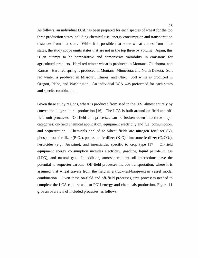
As follows, an individual LCA has been prepared for each species of wheat for the top
three production states including chemical use, energy consumption and transportation
distances from that state. While it is possible that some wheat comes from other
states, the study scope omits states that are not in the top three by volume. Again, this
is an attempt to be comparative and demonstrate variability in emissions for
agricultural products. Hard red winter wheat is produced in Montana, Oklahoma, and
Kansas. Hard red spring is produced in Montana, Minnesota, and North Dakota. Soft
red winter is produced in Missouri, Illinois, and Ohio. Soft white is produced in
Oregon, Idaho, and Washington. An individual LCA was preformed for each states
and species combination.
Given these study regions, wheat is produced from seed in the U.S. almost entirely by
conventional agricultural production [16]. The LCA is built around on-field and off-
field unit processes. On-field unit processes can be broken down into three major
categories: on-field chemical application, equipment electricity and fuel consumption,
and sequestration. Chemicals applied to wheat fields are nitrogen fertilizer (N),
phosphorous fertilizer (P2O5), potassium fertilizer (K2O), limestone fertilizer (CaCO3),
herbicides (e.g., Atrazine), and insecticides specific to crop type [17]. On-field
equipment energy consumption includes electricity, gasoline, liquid petroleum gas
(LPG), and natural gas. In addition, atmosphere-plant-soil interactions have the
potential to sequester carbon. Off-field processes include transportation, where it is
assumed that wheat travels from the field in a truck-rail-barge-ocean vessel modal
combination. Given these on-field and off-field processes, unit processes needed to
complete the LCA capture well-to-POU energy and chemicals production. Figure 11
give an overview of included processes, as follows.

29
29
Figure 11 – LCA process diagram
2.2.2 On-Field Chemical Application The USDA maintains a yearly inventory for volume of nitrogen, phosphorus,
potassium, and limestone fertilizers, in addition to herbicides and insecticides in its
Agricultural Chemical Usage Summary [17]. The USDA tabulates volumes of active
ingredients applied for winter, spring, and durum wheat in lbs/acre at the spatial
resolution of one American state. Here, it is assumed that the winter or spring variety
is applicable to primary species produced in that state, although it is not explicitly
stated in the report [17]. For example, it assumed that winter wheat from the state of

30
30
Ohio is soft red winter, which is the primary species produced in that state [25]. The
complete chemical volumes are listed in Appendix B. Values for each chemical were
converted to SI units (kg/ha) assuming 1 lb = 2.20 kg and 1 hectare (ha) = 2.47 acres
[58]. An extraction for applicable states is listed in Table 6.
Table 6 – Chemical application by wheat species, state, and active ingredient.
Spring Wheat Pesticides lb/acre kg/ha Idaho Nitrogen 1.21E+02 1.36E+02 Phosphate 4.10E+01 4.60E+01 Potash 3.70E+01 4.15E+01 Minnesota Nitrogen 1.08E+02 1.21E+02 Phosphate 4.90E+01 5.49E+01 Potash 3.80E+01 4.26E+01 Montana Nitrogen 5.70E+01 6.39E+01 Phosphate 3.50E+01 3.92E+01 Potash 2.20E+01 2.47E+01 North Dakota Nitrogen 1.14E+02 1.28E+02 Phosphate 5.00E+01 5.60E+01 Potash 2.40E+01 2.69E+01 Oregon Nitrogen 5.90E+01 6.61E+01 Phosphate 3.40E+01 3.81E+01 Potash 3.40E+01 3.81E+01 South Dakota Nitrogen 9.00E+01 1.01E+02 Phosphate 4.90E+01 5.49E+01 Potash 2.80E+01 3.14E+01 Washington Nitrogen 8.60E+01 9.64E+01 Phosphate 2.10E+01 2.35E+01 Potash 4.30E+01 4.82E+01 Total Nitrogen 9.80E+01 1.10E+02 Phosphate 4.60E+01 5.16E+01 Potash 2.90E+01 3.25E+01 Herbicides 5.58E-01 6.30E-01 Insecticide 4.00E-03 0.00E+00 Fungicide 2.20E-02 2.00E-02

31
31
Table 6 continued
Winter Wheat Colorado Nitrogen 3.80E+01 4.26E+01 Phosphate 2.30E+01 2.58E+01 Potash 2.50E+01 2.80E+01 Idaho Nitrogen 1.34E+02 1.50E+02 Phosphate 4.00E+01 4.48E+01 Potash 2.60E+01 2.91E+01 Illinois Nitrogen 1.15E+02 1.29E+02 Phosphate 9.40E+01 1.05E+02 Potash 1.30E+02 1.46E+02 Kansas Nitrogen 8.70E+01 9.75E+01 Phosphate 4.50E+01 5.04E+01 Potash 3.70E+01 4.15E+01 Michigan Nitrogen 1.15E+02 1.29E+02 Phosphate 5.90E+01 6.61E+01 Potash 7.50E+01 8.41E+01 Missouri Nitrogen 1.24E+02 1.39E+02 Phosphate 6.00E+01 6.73E+01 Potash 7.80E+01 8.74E+01 Montana Nitrogen 4.70E+01 5.27E+01 Phosphate 3.00E+01 3.36E+01 Potash 1.00E+01 1.12E+01 Nebraska Nitrogen 5.70E+01 6.39E+01 Phosphate 3.10E+01 3.48E+01 Potash 2.20E+01 2.47E+01 Ohio Nitrogen 1.00E+02 1.12E+02 Phosphate 7.50E+01 8.41E+01 Potash 8.40E+01 9.42E+01 Oklahoma Nitrogen 1.00E+02 1.12E+02 Phosphate 3.90E+01 4.37E+01 Potash 2.60E+01 2.91E+01 Oregon Nitrogen 8.20E+01 9.19E+01 Phosphate 5.70E+01 6.39E+01

32
32
Potash 5.00E+01 5.60E+01 South Dakota Nitrogen 8.30E+01 9.30E+01 Phosphate 4.70E+01 5.27E+01 Potash 4.30E+01 4.82E+01 Texas Nitrogen 8.60E+01 9.64E+01 Phosphate 5.30E+01 5.94E+01 Potash 1.70E+01 1.91E+01 Washington Nitrogen 9.30E+01 1.04E+02 Phosphate 2.70E+01 3.03E+01 Potash 2.80E+01 3.14E+01 Total Nitrogen 8.80E+01 9.86E+01 Phosphate 4.60E+01 5.16E+01 Potash 5.80E+01 6.50E+01 Herbicides 2.49E-01 2.80E-01 Insecticide 2.00E-02 2.00E-02 Fungicide 3.00E-03 0.00E+00
As described in the literature review, on-farm application of fertilizers and chemicals
were among the largest contributors to life cycle greenhouse gas emissions.
2.2.3 On-Field Equipment Energy Consumption and Emissions
Similarly, the USDA compiles detailed energy use in the agriculture industry. The
Energy Use on Major Field Crops in Surveyed States report tracks fuel consumption
for wheat, corn, rice, soybean, sugar beet, and cotton cultivation for each American
state [22]. Gasoline (gallons/acre), diesel (gallons/acre), liquid petroleum gas
(gallons/acre), electricity (kWh/acre), and natural gas (cubic ft/acre) use are included
for all fossil fuel-based farm operations. Farm machinery operations cover all on-farm
processes that consumer fossil fuels, including tractor and farm truck use, irrigation,
and drying of grain [22]. A complete account is included in Appendix C. An
extraction for study states and conversion to SI units (assuming 1 gal = 3.79 L, 1
hectare (ha) = 2.47, and 1ft3 = 0.028 m3) [58] is presented in Table 7. Field practices,
and consequently energy use and fossil fuel consumption, vary widely by state. For

33
33
example, several states consume no electricity, while Idaho uses over 1.01E+03
kWh/ha wheat. Washington consumes as much as 5.14E+01 L/ha of diesel fuel, while
Illinois consumes as little as 1.87E+01 L/ha of diesel fuel. Emissions for each fuel
type, including electricity, are quantified in Section 2.2.6 using the Department of
Energy Argonne National Laboratory’s Greenhouse Gases, Regulated Emissions, and
Energy Use in Transportation (GREET) LCA Model [59].
Table 7 – Energy consumption for 1 ha wheat by American state. Shading indicated states included in system boundary.
Diesel Gasoline LPG Electricity Natural gas L/ha L/ha L/ha kWh/ha m3/ha Colorado 4.21E+01 1.31E+01 0.00E+00 2.20E+00 0.00E+00 Georgia 4.40E+01 1.31E+01 0.00E+00 0.00E+00 0.00E+00 Idaho 4.49E+01 1.40E+01 0.00E+00 1.01E+03 0.00E+00 Illinois 1.87E+01 1.59E+01 0.00E+00 0.00E+00 0.00E+00 Kansas 4.30E+01 8.40E+00 8.40E+00 0.00E+00 0.00E+00 Louisiana 4.58E+01 2.43E+01 0.00E+00 0.00E+00 0.00E+00 Minnesota 3.74E+01 9.40E+00 1.90E+00 0.00E+00 0.00E+00 Mississippi 3.37E+01 1.40E+01 0.00E+00 0.00E+00 0.00E+00 Missouri 4.12E+01 1.59E+01 0.00E+00 7.20E+00 0.00E+00 Montana 3.18E+01 9.40E+00 0.00E+00 2.69E+01 0.00E+00 Nebraska 4.58E+01 7.50E+00 0.00E+00 0.00E+00 0.00E+00 North Carolina 3.74E+01 2.99E+01 0.00E+00 1.50E+00 0.00E+00 North Dakota 3.37E+01 9.40E+00 0.00E+00 1.11E+01 0.00E+00 Ohio 2.15E+01 1.59E+01 0.00E+00 6.70E+00 0.00E+00 Oklahoma 5.33E+01 6.50E+00 0.00E+00 0.00E+00 0.00E+00 Oregon 5.80E+01 2.34E+01 0.00E+00 5.07E+01 0.00E+00 South Dakota 2.81E+01 7.50E+00 0.00E+00 0.00E+00 0.00E+00 Texas 4.77E+01 6.50E+00 1.19E+01 3.11E+01 1.00E-01 Washington 5.14E+01 1.22E+01 0.00E+00 4.03E+01 0.00E+00
2.2.4 Yield Yield for each state and wheat species combination were extracted from the USDA
summary on grain production and are displayed in Table 8 [25]. Complete yield
information is included in Appendix A.

34
34
Table 8 – Wheat yield in kg/ha for each location and species.
Species States Yield (kg/ha) Hard Red Winter Montana 2.80E+03 Kansas 2.34E+03 Oklahoma 1.95E+03 Hard Red Spring Montana 1.84E+03 Minnesota 3.10E+03 North Dakota 2.30E+03 Soft Red Winter Missouri 3.47E+03 Illinois 4.05E+03 Ohio 4.36E+03 Soft White Oregon 3.51E+03 Idaho 5.33E+03 Washington 3.80E+03
2.2.5 Transportation Mode, Distance, and Load Factors Transportation modes are generally separated into water, land, or air transport in LCA
studies. Intermodal transportation (a combination of one or more modes) is used to
transport agricultural bulk freight from field to the POU. Fuel consumption, emissions
associated with fuel combustion, cargo spills, noise pollution, and land use from
highways, ports, rail development are environmental issues resulting from
transportation [60]. The materials acquisition, fuel processing and transport,
maintenance of vehicles, and end-of-life processes are also important for an LCA
study [61].
A robust model of the wheat supply chain is possible because of a well-documented
infrastructure and path to export in the U.S.. Wheat, in addition to corn and soybeans,
has been exported from the U.S. for over 100 years [45]. The longevity of the grain

35
35
industry gives it an established local infrastructure for moving wheat from the field to
market. Wheat is usually grown within a 100km distance from a regional distribution
facility in both the northwest and the central plains region [62], [63]. This distance is
an upper quartile estimate, so it is unlikely that grain travels longer than 100km by
truck [63]. These facilities are often referred to as “grain bins.” In the case of wheat
destined for Japan, the wheat continues from local bins by Class I diesel freight train
bulk hopper to port of export in Portland, Oregon (Figure 12). Containerized transport
of grain currently occupies a small market niche of grain exports (>5%) [64]. This
LCA assumes all grain travels solely by covered bulk hopper. From the port, wheat is
transported predominantly on Panamax or Handymax bulk ocean vessels to POU in
Yokohama, Japan [37], [65]. Currently, Port of Portland is the only port facility that
exports large volumes of wheat to Asia, which restricts both the domestic and ocean
transportation routes [66]. One exception to the truck-rail-ocean vessel modal
combination is in the case of soft white wheat produced in the northwest U.S., where it
is assumed that wheat is moved by barge on the Columbia River a distance of 350 km
[62].

36
36
Figure 12 – U.S. wheat bin locations.
For this LCA, each species of wheat has three production states with different paths to
market in Japan [37]. It was assumed that wheat travels by bulk Class 6 trucks from
farms to local bins at a distance of 100km [62]. This estimate is consistent for grain in
the northwest and plains [62], [63]. The rail distances for each state bin to Port of
Portland was calculated exactly using the Network Analyst extension in ESRI’s
ArcGIS software package and the U.S. Department of Transportation GIS database
[67]. The ocean distance is assumed to be vessels at a distance of 8,000 km, based on
AIST’s LCA database.
In addition to the distances for each mode, transportation methodology developed in
the Design for Environment laboratory at the University of Washington requires an
accurate representation of backhaul (or return trip) assumptions for each mode [68],
[69]. Here, domestic rail, truck, and barge are assumed to have a 100% empty
backhaul (i.e., all vehicles and vessels return empty form the destination to the point of
origin). Tight capacity, specialized grain containers, and non-existent demand for
grain movement back into the American heartland forces all hoppers to currently be

37
37
sent back empty [66]. This assumption has been confirmed by Herland Ugles,
president of the International Longshore and Warehouse Union Local 19, and Bruce
Agnew, Program Director of the Cascadia Transportation Group in personal
communications [70], [71].
For ocean transport to Japan, Panamax and Handymax vessels calling from Asia ports
return to America ports near capacity [70]. Vessels are carrying predominantly
finished bulk goods such as metals, clean paper pulp, minerals, and even specialty
grain [72]. There's a slight imbalance in trade for bulk good (20%), with exports from
the U.S. still being higher [72]. Because it is unclear from personal communications
with Herland Ugles that a consistent backhaul pattern exists for ships used for U.S.
grain, it is assumed here that ocean transport of wheat to Japan has 0% empty
associated backhaul [70]. This decision was made in an effort to be conservative in
backhaul assumptions for ocean transport where a clear pattern is not known.
Calculated transportation distances, including backhaul, for each state are listed in
Table 9.

38
38
Table 9 – Transportation distances for each mode including fronthaul and backhaul.
Class 6 Truck
(km) Rail (km) Barge (km) Bulk Ocean Vessel
(km)
Fronthaul 1.00E+02 1.35E+03 0.00E+00 8.00E+03
Montana Backhaul 1.00E+02 1.35E+03 0.00E+00 0.00E+00
Fronthaul 1.00E+02 2.86E+03 0.00E+00 8.00E+03
Kansas Backhaul 1.00E+02 2.86E+03 0.00E+00 0.00E+00
Fronthaul 1.00E+02 3.43E+03 0.00E+00 8.00E+03
Oklahoma Backhaul 1.00E+02 3.43E+03 0.00E+00 0.00E+00
Fronthaul 1.00E+02 2.75E+03 0.00E+00 8.00E+03
Minnesota Backhaul 1.00E+02 2.75E+03 0.00E+00 0.00E+00
Fronthaul 1.00E+02 2.08E+03 0.00E+00 8.00E+03
North Dakota Backhaul 1.00E+02 2.08E+03 0.00E+00 0.00E+00
Fronthaul 1.00E+02 2.86E+03 0.00E+00 8.00E+03
Missouri Backhaul 1.00E+02 2.86E+03 0.00E+00 0.00E+00
Fronthaul 1.00E+02 3.36E+03 0.00E+00 8.00E+03
Illinois Backhaul 1.00E+02 3.36E+03 0.00E+00 0.00E+00
Fronthaul 1.00E+02 3.82E+03 0.00E+00 8.00E+03
Ohio Backhaul 1.00E+02 3.82E+03 0.00E+00 0.00E+00
Fronthaul 1.00E+02 3.00E+02 3.50E+02 8.00E+03
Oregon Backhaul 1.00E+02 3.00E+02 3.50E+02 0.00E+00
Fronthaul 1.00E+02 6.00E+02 3.50E+02 8.00E+03
Idaho Backhaul 1.00E+02 6.00E+02 3.50E+02 0.00E+00
Fronthaul 1.00E+02 3.00E+02 3.50E+02 8.00E+03
Washington Backhaul 1.00E+02 3.00E+02 3.50E+02 0.00E+00
Load factor assumptions for wheat fronthaul are assumed to be 100% for rail, barge,
and truck fronthauls [59]. Domestic backhaul load factors are assumed to be 0%.
Ocean fronthaul load factor is modified to 100% based on personal communication
with Harold Ugles at the ILWU [70].
2.2.6 Well-to-Point-of-Use Energy and Chemicals Production
Given equipment energy use and emissions, chemical application and emissions, and
transportation modes, distances, and load factors for wheat, the Department of Energy
Argonne National Laboratory’s Greenhouse Gases, Regulated Emissions, and Energy
Use in Transportation (GREET) Model version 1.7 was used for LCA process
information. GREET estimates life cycle energy consumption (as the total energy,
fossil, and petroleum use) and emissions of CO2 in addition to other greenhouse gas

39
39
and particulate emissions. GREET applications to date are primarily assessments of
transportations systems (personal and fuel cell vehicles), but what is of value here are
the fuel cycle, electricity production, logistics models (transport on land, through
inland waters, or by sea), and agricultural equipment and chemicals contained within
GREET. In particular, GREET’s analysis of biofuels produces robust, and American-
specific process information for all agricultural chemicals used for wheat production
and included in the study scope.
There are at least three advantages of using GREET. First, the data and model results
are well developed and documented, have been highly peer reviewed, and are widely
accepted by LCA practitioners [68]. Combination of GREET emissions with USDA
consumption records and robust transportation distances allows a detailed and clear
understanding of variation in emissions for wheat export. Second, using only GREET
for process information standardizes U.S. emissions data sources. Lastly, the GREET
system’s extensive set of fuel cycle parameters are easily modified, allowing exact
load factors for transportation, local electricity profiles, and modification if U.S.
energy, fertilizer production changes. This allowed an individual electricity mix to be
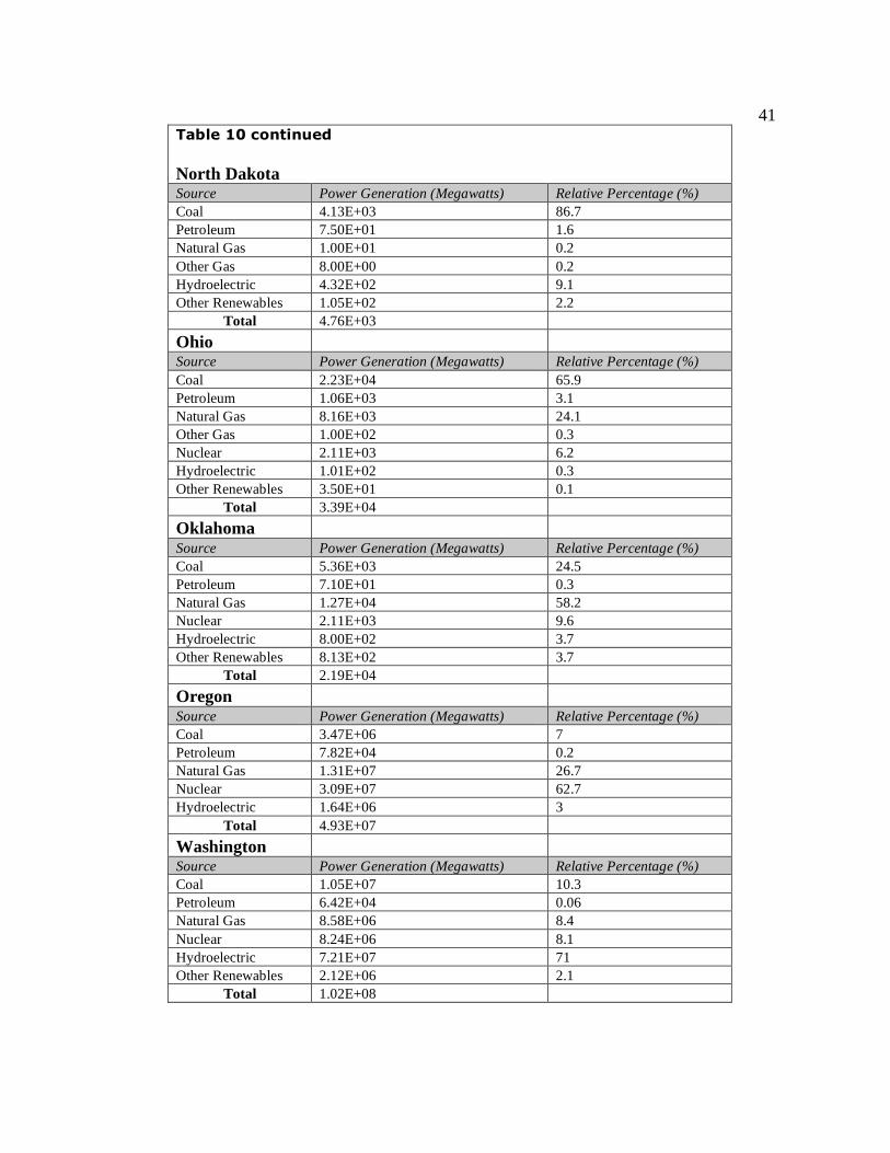
used for wheat produced in that state. Electricity profiles are listed in Table 10.

40
40
Table 10 – Electricity profile for each wheat production state.
Idaho Source Power Generation (Megawatts) Relative Percentage (%) Coal 1.70E+01 0.5 Petroleum 5.00E+00 0.2 Natural Gas 6.45E+02 20.4 Hydroelectric 2.39E+03 75.6 Other Renewables 8.80E+01 2.8 Other 1.50E+01 0.5
Total 3.16E+03
Illinois Source Power Generation (Megawatts) Relative Percentage (%) Coal 1.58E+04 37 Petroleum 1.15E+03 3 Natural Gas 1.39E+04 32.6 Other Gas 4.70E+01 0 Nuclear 1.14E+04 26.8 Hydroelectric 3.30E+01 0.1 Other Renewables 2.52E+02 0.6
Total 4.25E+04
Kansas Source Power Generation (Megawatts) Relative Percentage (%) Coal 5.25E+03 47.6 Petroleum 5.83E+02 5.3 Natural Gas 3.76E+03 34.1 Nuclear 1.17E+03 10.6 Other Renewables 2.63E+02 2.4
Total 1.10E+04
Minnesota Source Power Generation (Megawatts) Relative Percentage (%) Coal 5.45E+03 45 Petroleum 7.39E+02 6.1 Natural Gas 3.16E+03 26.1 Nuclear 1.62E+03 13.4 Hydroelectric 1.76E+02 1.5 Other Renewables 9.60E+02 7.9
Total 1.21E+04
Missouri Source Power Generation (Megawatts) Relative Percentage (%) Coal 1.13E+04 54.9 Petroleum 1.25E+03 6.1 Natural Gas 5.61E+03 27.3 Nuclear 1.19E+03 5.8 Hydroelectric 5.52E+02 2.7 Other Renewables 6.57E+02 3.2
Total 2.05E+04
41
41
Table 10 continued
North Dakota Source Power Generation (Megawatts) Relative Percentage (%) Coal 4.13E+03 86.7 Petroleum 7.50E+01 1.6 Natural Gas 1.00E+01 0.2 Other Gas 8.00E+00 0.2 Hydroelectric 4.32E+02 9.1 Other Renewables 1.05E+02 2.2
Total 4.76E+03
Ohio Source Power Generation (Megawatts) Relative Percentage (%) Coal 2.23E+04 65.9 Petroleum 1.06E+03 3.1 Natural Gas 8.16E+03 24.1 Other Gas 1.00E+02 0.3 Nuclear 2.11E+03 6.2 Hydroelectric 1.01E+02 0.3 Other Renewables 3.50E+01 0.1
Total 3.39E+04
Oklahoma Source Power Generation (Megawatts) Relative Percentage (%) Coal 5.36E+03 24.5 Petroleum 7.10E+01 0.3 Natural Gas 1.27E+04 58.2 Nuclear 2.11E+03 9.6 Hydroelectric 8.00E+02 3.7 Other Renewables 8.13E+02 3.7
Total 2.19E+04
Oregon Source Power Generation (Megawatts) Relative Percentage (%) Coal 3.47E+06 7 Petroleum 7.82E+04 0.2 Natural Gas 1.31E+07 26.7 Nuclear 3.09E+07 62.7 Hydroelectric 1.64E+06 3
Total 4.93E+07
Washington Source Power Generation (Megawatts) Relative Percentage (%) Coal 1.05E+07 10.3 Petroleum 6.42E+04 0.06 Natural Gas 8.58E+06 8.4 Nuclear 8.24E+06 8.1 Hydroelectric 7.21E+07 71 Other Renewables 2.12E+06 2.1
Total 1.02E+08

42
42
Table 11 displays process information for fronthaul study transportation processes.
Relevant modes include bulk ocean carriers, transport barge, diesel freight train,
medium-heavy truck, with included fuel production processes. On wheat fronthaul,
the grain industry is currently operating at capacity [66]. GREET load factors are set
at a default of 80% [59] for all modes except rail. However, this was modified here to
a 100% load factor to match conditions for wheat. Cargo payloads and mile per gallon
estimates were left unmodified from GREET defaults [59].
Table 12 displays process information for backhaul study transportation processes.
Again, relevant modes include transport barge, diesel freight train, medium-heavy
truck, with included fuel production processes. Again, note that bulk ocean carriers
are assumed to have no associated backhaul and are not included. For wheat
backhaul, the grain industry has an assumed 100% empty backhaul for barge, rail, and
truck due to high demand for grain hoppers in the American plains and Midwest [70].
Therefore, the load factor is 0%, with payload and mile per gallon left unmodified.
Table 13 displays process information for on-site fuel use and energy production.
GREET’s focus on fuel and transportation systems is particularly useful for on-site
fuel use. It includes diesel and gasoline combusted specifically in a farming tractor.
On-site electricity, natural gas, and LPG consumption and associated fuel production
processes are also included. GREET allows a modification of the electricy
contribution mix, which was altered to match the generation profile for each wheat
producing state. Each state has a different relative contribution of coal, petroleum,
natural gas, hydroelectric, and other renewables [23].
Table 14 displays process information for chemical application. Nitrogen, P2O5, K2O,
CaCO3 fertilizer are included in GREET for each gram of active nutrient. Pesticides,
insecticides, and herbicides are also included. It is important to note that GREET
accounts for the direct emissions of N2O from fertilized soil [59].

43
Table 11 – Summary of energy use and emissions for fronthaul transportation modes.
Product Bulk Carriers, 45,000 dwt- 100% load
Transport- Barge, average payload 1,500
tons (U.S.), 80% load
Transport by Diesel Freight Train (U.S.),
Transport by Medium-Heavy Truck- class 6 or 7 (8 ton cargo), 7.3mpg, 100%
load,
Residual Oil, at
refueling station
Diesel for non-road
engines, at fueling station
Conventional and LS Diesel, at
fueling station
ECONOMIC FLOWS Product quantity 1.00E+00 1.00E+00 1.00E+00 1.00E+00 Product quantity units of measure kg-km kg-km kg-km kg-km Residual Oil, at refueling station BTU -2.76E-01 1.00E+06 Diesel for non-road engines, at fueling station BTU -2.53E-01 1.00E+06 Conventional and LS Diesel, at fueling station BTU -1.51E+00 1.00E+06 Bunker fuel BTU -7.12E-02 ENVIRONMENTAL FLOWS CO2 g 6.04E-03 2.34E-02 1.97E-02 1.17E-01 8.36E+03 1.45E+04 1.66E+04 CH4 g 4.09E-08 5.26E-07 9.99E-07 2.31E-06 9.62E+01 1.03E+02 1.05E+02 N2O g 1.42E-07 5.52E-07 5.07E-07 4.37E-06 1.48E-01 2.41E-01 2.74E-01

44
Table 12 – Summary of energy use and emissions for backhaul transportation modes.
Product
Transport- Barge, average payload 1,500 tons (U.S.), 0% load
Transport by Diesel Freight Train (U.S.),
Transport by Medium-Heavy Truck- class 6 or 7 (8 ton cargo), 7.3mpg, 0% load,
Residual Oil, at refueling station
Diesel for non-road engines, at fueling station
Conventional and LS Diesel, at fueling station
ECONOMIC FLOWS Product quantity 1.00E+00 1.00E+00 1.00E+00 Product quantity units of measure kg-km kg-km kg-km Residual Oil, at refueling station BTU -1.35E-02 1.00E+06 Diesel for non-road engines, at fueling station BTU -2.53E-01 1.00E+06 Conventional and LS Diesel, at fueling station BTU -1.02E+00 1.00E+06 Bunker fuel BTU ENVIRONMENTAL FLOWS CO2 g 1.31E-03 1.97E-02 7.98E-02 8.36E+03 1.45E+04 1.66E+04 CH4 g 1.12E-06 9.99E-07 1.57E-06 9.62E+01 1.03E+02 1.05E+02 N2O g 2.70E-08 5.07E-07 2.97E-06 1.48E-01 2.41E-01 2.74E-01

45
Table 13 – Summary of energy use and emissions for on-site energy production.
Product
Stationary Grid
Electricity, at POU
Natural Gas burned in a Stationary
Reciprocating Engine: urban
facility, at POU
Diesel Fuel
burned in a Farming Tractor: urban
farm, at POU
Gasoline burned in a
Farming Tractor:
urban farm, at POU
Natural Gas as a
Stationary Fuel, at POU
Natural Gas for
electricity generation,
at POU
Diesel, at POU
Gasoline, at POU
LPG, at POU
ECONOMIC FLOWS Product quantity 1.00E+06 1.00E+06 1.00E+06 1.00E+06 1.00E+06 1.00E+06 1.00E+06 1.00E+06 1.00E+06 Product quantity units of measure BTU BTU BTU BTU BTU BTU BTU BTU BTU Natural Gas as a Stationary Fuel, at POU BTU 0.00E+00 -1.00E+06 0.00E+00 0.00E+00
as product quant. 0.00E+00 0.00E+00 0.00E+00 0.00E+00
Natural Gas for electricity generation, at POU BTU 0.00E+00 0.00E+00 0.00E+00 0.00E+00 0.00E+00
as product quant. 0.00E+00 0.00E+00 0.00E+00
Residual Oil, at POU BTU 0.00E+00 0.00E+00 0.00E+00 0.00E+00 0.00E+00 0.00E+00 0.00E+00 0.00E+00 0.00E+00
Diesel, at POU BTU 0.00E+00 0.00E+00 -1.00E+06 0.00E+00 0.00E+00 0.00E+00
as product quant. 0.00E+00 0.00E+00
Gasoline, at POU BTU 0.00E+00 0.00E+00 0.00E+00 -1.00E+06 0.00E+00 0.00E+00 0.00E+00
as product quant. 0.00E+00
Crude, at POU BTU 0.00E+00 0.00E+00 0.00E+00 0.00E+00 0.00E+00 0.00E+00 0.00E+00 0.00E+00 0.00E+00
LPG, at POU BTU 0.00E+00 0.00E+00 0.00E+00 0.00E+00 0.00E+00 0.00E+00 0.00E+00 0.00E+00
as product quant.
ENVIRONMENTAL FLOWS CO2 g 2.20E+05 5.77E+04 7.74E+04 7.56E+04 5.24E+03 5.16E+03 1.45E+04 1.78E+04 1.02E+04 CH4 g 2.96E+02 3.69E+02 6.30E-01 5.19E+00 1.96E+02 1.75E+02 1.03E+02 1.07E+02 9.83E+01 N2O g 3.12E+00 1.50E+00 9.20E-01 1.10E+00 8.55E-02 8.32E-02 2.41E-01 2.91E-01 1.76E-01

46
Table 14 – Summary of Energy Use and Emissions of Agricultural Chemicals
Fertilizer (per gram of nutrient)
Herbicides: Average for Crop Type
Pesticides: Average for Crop Type
Insecticides: Average for Crop Type
Nitrogen P2O5 K2O CaCO3 Wheat Wheat Corn Quantity of Fertilizer (grams) 1.00E+00 1.00E+00 1.00E+00 1.00E+00 1.00E+00 1.00E+00 1.00E+00 Total Emissions: grams per gram CH4 2.60E-03 1.50E-03 7.00E-04 6.00E-04 2.00E-02 2.00E-02 2.82E-02 N2O 1.60E-03 0.00E+00 0.00E+00 0.00E+00 0.00E+00 0.00E+00 2.00E-04 CO2 2.20E+00 7.54E-01 4.13E-01 3.56E-01 1.61E+01 1.61E+01 1.85E+01

47
47
2.2.7 Accounting for System Co-Products Grain cultivation in the U.S. produces two products: wheat grain and wheat straw [73].
As indicated by the standards, system expansion is the preferred method for
addressing multifunctional processes However, because there is no mono-functional
process to produce wheat straw, allocation of on-field processes and sequestration
credits was preformed based on the economic percentage of the two co-products.
Each individual wheat species has a slightly different percentage of wheat grain and
straw. Table 15 lists the allocation percentages from the USDA’s Characteristics of
U.S. Wheat Farming report [73]. According to the report, farms of different value
(high, medium, and low) have a different economic percentage of wheat straw vs.
wheat grain. Furthermore, each region where wheat is grown has a different
distribution of high, medium, and low value farms. An allocation for each species of
wheat was calculated by multiplying the disruption of farm value per species by the
economic percentage for each value of farm. Note that an allocation was only
preformed for the production, and not the transportation of grain.
Table 15 – Allocation for wheat and straw by species.
Species Wheat Grain Straw White 96.2% 3.8% Hard Red Winter 95.5% 4.5% Hard Red Spring 94.7% 5.3% Soft Red Winter 95.6% 4.4%
2.2.8 Sequestration A complete agricultural LCA for the quantification of contribution to climate change
must correctly address the potential of wheat fields to sequester carbon. A review of
carbon sequestration potential for wheat cultivation is presented in Table 16. The
range is remarkable, at -1404 kg CO2 eq./ha to 1440 kg CO2/ha per year sequestered,

48
48
and underscores variability of the range of 152 to 1330 g CO2 eq/kg wheat presented
in Table 4.
Table 16 – Carbon sequestration of wheat cultivation in kg CO2/ha
kg CO2/ha per year sequestered Study Method Cultivation Method Reference
-1404 Direct Flux Measurement Conventional Kessavalou, et al. [34] -1548 Direct Flux Measurement Reduced Tillage Kessavalou, et al. [34] -1764 Direct Flux Measurement No Tillage Kessavalou, et al. [34]
294 Carbon Tracer Conventional Tillage Gregory and Atwell [74] 612 Carbon Tracer Conventional Tillage Kuzyakov, et al. [30] 750 Carbon Tracer Conventional Tillage Markin & Puckridge [75] 796 Carbon Tracer Conventional Tillage Keith et al. [76]
1080 Carbon Tracer Conventional Tillage Martin & Merckx [77] 1100 Carbon Tracer Conventional Tillage Martin & Merckx [77] 1140 Carbon Tracer Conventional Tillage Swinnen, et al. [78] 1250 Carbon Tracer Conventional Tillage Whipps, et al. [79] 1290 Direct Flux Measurement Reduced Tillage Curtin, et al. [28] 1320 Direct Flux Measurement Reduced Tillage Majumder, et al.[80] 1410 Carbon Tracer Conventional Tillage Johnen & Sauerbeck [81] 1440 Direct Flux Measurement Reduced Tillage Purakayastha, et al. [35]
2.2.9 Major Assumptions and Limitations
Assumptions and limitations have been stated in methodological context, but should
also be stated explicitly. Significant limitations include exclusions from the system
boundary, narrow scope, impacts, and transportation assumptions.
• This LCA is applicable to the current production and transportation conditions
in the U.S. for levels of energy use, fertilizer application, and electric
generation mix. It represents a single point in time to compare different
production locations for the same class of agricultural product. The U.S.
agricultural industry as a whole is characterized by extremely volatile market
shares, availability, prices, and yield [37]. Both the location of origin and
regional energy and chemical field practices for American wheat exported to
Japan is annually variable [53]. However, it is assumed that distributed market
share of wheat production is consistent with wheat for export to Japan at the

49
49
spatial scale of one American state. When data were available for multiple
crop years, such as yield, values used for LCA calculation were averaged to
account for yearly variation [25].
• The study does not account for every method that wheat can be produced and
transported. Results are intended to inform LCA practitioners on the potential
variation of environmental impact in crop production and are limited spatially
by the available USDA data.
• In the case of multiple modes of transportation in the same location, the most
common method was used. For example, wheat from the central U.S. can
travel by Columbia River barge or train, but barge is predominantly used for
soft white wheat from the northwest [62]. Assumptions for modes, backhauls,
and distances are based on current grain infrastructure, USDA data, and
communication with grain experts [65], [70]. Shifts in port of export, increase
in the use of containerized grain, or increase in bulk hopper capacity could
change the modeled transportation processes.
• Process information for chemicals application, fuel use, and transportation are
much better understood that sequestration of wheat fields. However, a
comparison with applicable SOC data are presented in the discussion.
• Farm, infrastructure, and equipment construction have not been included.
• Impact analysis is limited to greenhouse gas emissions only. Ideally, all
impact categories should be included (as eutrophication, loss of habitat and
biodiversity, changes in land use and disturbance, heavy metal soil release as
noted in Section 1.2), but only greenhouse gases were quantified here. This is
consistent with the ISO standards to tailor impact assessment to primary study
goals [3].

50
50
2.3 Impact Assessment Impact assessment includes contribution to global warming from emissions of CO2,
CH4, and N2O and carbon sequestration. The IPCC Fourth Assessment developed the
global warming potentials (GWPs) used to calculate the contribution of each emission
type to global warming relative to the contribution of emissions of CO2 [82]. For
example, the most recent report equates 1 unit of CO2 to 25 units of CH4 in terms of
climate forcing (Table 17). In the impact assessment, the life cycle emissions and
sequestration of each gas estimated in the inventory analysis is multiplied by the
respective GWP and summed to obtain an estimate of the life cycle total.
Table 17 – Global Warming Potentials (GWPs)
Emission CO2 Equivalent (100 Years)
CO2 1
CH4 25
N2O 298
2.4 Case Study Results
2.4.1 Results By State Case study results for wheat production were calculated for each wheat species from
the top three production states as described above. This combines USDA crop
production usage with LCA emissions from the GREET database. Table 18 presents
an example for Hard Red Winter wheat from Montana. The initial data sources from
the USDA report production inputs per hectare. For example, nitrogen fertilizer is
kg/ha and diesel use is L/ha. Since the functional unit for the LCA is 1 kg dry wheat,
inputs must be converted using each state’s wheat yield (assuming conversion factors
of 2.47 ha per acre and 25.43 kg per bushel dry wheat [83] and varied in the
interpretation Section 2.4.5). Here, for clear presentation, emissions for each

51
51
economic flow include their associated processes and are referred to as intensity. This
process was repeated for each species and state combination in Appendix D.
Table 18 – Inventory results for hard red winter wheat from Montana. Grey shading indicates the two largest contributors to total greenhouse gas emissions.
MONTANA - Hard Red Winter
YIELD 43 Bushels/acre
Process Input Unit
Input (normalized to yield) Unit Intensity Unit
Process Reference
CO2 Emission (gCO2 eq./kg Wheat)
Relative %
Nitrogen fertilizer (N)
5.27E+01 kg/ha
1.88E-02
kg fertilizer/kg Wheat
2.94E+00
kg CO2/kg fertilizer
GREET 1.7 5.54E+01 39.0%
Phosphorous fertilizer (P2O5)
3.36E+01 kg/ha
1.20E-02
kg/kg Wheat 6.70E-01
kg CO2/kg fertilizer
GREET 1.7 8.06E+00 5.7%
Potassium Fertilizer (K2O)
1.12E+01 kg/ha
4.01E-03
kg/kg Wheat 9.90E-01
kg CO2/kg fertilizer
GREET 1.7 3.97E+00 2.8%
Limestone 4.48E+01 kg/ha
1.60E-02
kg/kg Wheat 6.10E-01
kg CO2/kg fertilizer
GREET 1.7 9.78E+00 6.9%
Herbicides 2.80E-01 kg/ha
1.00E-04
kg/kg Wheat
2.08E+01
kg CO2/kg herbacide
GREET 1.7 2.08E+00 1.5%
Insecticides 2.01E-02 kg/ha
7.18E-06
kg/kg Wheat
2.43E+01
kg CO2/kg insecticides
GREET 1.7 1.74E-01 0.1%
Diesel!Farm machinery)
3.19E+01 L/ha
1.14E-02
L/kg Wheat
3.35E+00
kg CO2/L consumed
GREET 1.7 3.82E+01 26.9%
Diesel (Custom operation)
7.79E+00 L/ha
2.79E-03
L/kg Wheat
3.35E+00
kg CO2/L consumed
GREET 1.7 9.34E+00 6.6%
Electricity 2.69E+01
kWh/ha
9.63E-03
kWh/kg Wheat 5.34E-01
kg CO2/kWh
GREET 1.7 (assuming local mix) 5.15E+00 3.6%
Gasoline 9.37E+00 L/ha
3.35E-03
L/kg Wheat
2.97E+00
kg CO2/L consumed
GREET 1.7 9.96E+00 7.0%
LP Gas 0.00E+00 L/ha
0.00E+00
L/kg Wheat
2.84E+00
kg CO2/L consumed
GREET 1.7 0.00E+00 0.0%
Natural Gas
0.00E+00 m3/ha
0.00E+00
m3/kg Wheat
2.35E+00
kg CO2/m3 consumed
GREET 1.7 0.00E+00 0.0%
RAW TOTAL 1.42E+02
ALLOCATION 95.5%
TOTAL 1.36E+02

52
52
Inventory results for the transportation component are displayed in Table 19. This
combines fronthaul and backhauls distances from in Table 9 with LCA emissions from
the GREET database in Table 11 and Table 12. Distances are multiplied by life cycle
emissions from GREET, resulting in total transportation emissions by state. Again, in
GREET each economic flow for transportation (Class 6 Truck, Bulk Ocean Vessel)
has only one associated process for the fuel production. Therefore, emissions for the
two are combined for clear presentation in Table 19.
Table 19 – Life cycle emissions by state for transportation component.
FRONTHAUL BACKHAUL
Class 6 Truck (km)
Rail (km)
Barge (km)
Bulk Ocean Vessel (km)
Class 6 Truck (km)
Rail (km)
Barge (km)
Emissions (gCO2 eq/km) 1.41E-01 2.30E-02 2.60E-02 7.00E-03 8.10E-02 2.00E-02 2.00E-02
TOTAL (gCO2 eq/kg
wheat)
Oregon 1.00E+02 3.00E+02 3.50E+02 8.00E+03 1.00E+02 3.00E+02 3.50E+0
2 1.04E+0
2 Washington 1.00E+02 3.00E+02 3.50E+02 8.00E+03 1.00E+02 3.00E+02
3.50E+02
1.04E+02
Idaho 1.00E+02 6.00E+02 3.50E+02 8.00E+03 1.00E+02 6.00E+02 3.50E+0
2 1.17E+0
2
Montana 1.00E+02 1.35E+03 0.00E+00 8.00E+03 1.00E+02 1.35E+03 0.00E+0
0 1.34E+0
2 North Dakota 1.00E+02 2.08E+03 0.00E+00 8.00E+03 1.00E+02 2.08E+03
0.00E+00
1.65E+02
Minnesota 1.00E+02 2.75E+03 0.00E+00 8.00E+03 1.00E+02 2.75E+03
0.00E+00
1.94E+02
Kansas 1.00E+02 2.86E+03 0.00E+00 8.00E+03 1.00E+02 2.86E+03 0.00E+0
0 1.99E+0
2
Missouri 1.00E+02 2.86E+03 0.00E+00 8.00E+03 1.00E+02 2.86E+03 0.00E+0
0 1.99E+0
2
Illinois 1.00E+02 3.36E+03 0.00E+00 8.00E+03 1.00E+02 3.36E+03 0.00E+0
0 2.20E+0
2
Oklahoma 1.00E+02 3.43E+03 0.00E+00 8.00E+03 1.00E+02 3.43E+03 0.00E+0
0 2.23E+0
2
Ohio 1.00E+02 3.82E+03 0.00E+00 8.00E+03 1.00E+02 3.82E+03 0.00E+0
0 2.40E+0
2
Total inventory results for each species in each of the top three production states were
combined to form Table 20. Note that an economic allocation was performed on
wheat production values as listed in Table 15 for each species of wheat to account for

53
53
wheat straw co-production. Total life cycle emissions are the result of both
production and transportation to POU in Japan. Production ranged from a maximum of
272 g CO2 eq/kg wheat for hard red spring produced in North Dakota to a minimum of
136 g CO2 eq/kg wheat for hard red winter wheat from Montana. Transportation
varied from 104 g CO2 eq/kg for wheat delivered from Oregon and Washington, to
223 g CO2 eq/kg for wheat from Oklahoma. Intra-species variation for total
greenhouse gas emissions was as large as 101% for hard red winter and as little as 7%
for soft white.
Table 20 – Life cycle emissions for each species and state combination.
Production Production Transportation Total Hard Red Winter
(kgCO2 eq/ha)
(gCO2 eq/kg wheat)
(gCO2 eq/kg wheat)
(gCO2 eq/kg wheat)
Montana 379 136 134 269
Kansas 587 251 199 450
Oklahoma 617 316 223 540
Hard Red Spring
Minnesota 625 202 194 395
Montana 430 233 134 367
North Dakota 625 272 165 437
Soft Red Winter
Ohio 635 146 240 386
Illinois 730 180 145 326
Missouri 758 219 199 417
White
Idaho 811 152 117 269
Washington 608 160 104 264
Oregon 626 178 104 283
Results for carbon equivalent emissions in each state are displayed spatially using GIS
in Figure 13.

54
Figure 13 – Carbon equivalent emissions for each wheat species.

55
55
2.4.2 Results by Species Total emissions for each of the four species were derived by the relative percentage in
each of the top three production states following Design for Environment
methodology [84]. Figure 14 contains the relative production percentage of the top
three states for each wheat species. These were calculated based on total average yield
for each species for the 2005 and 2006 crop production years [25].
Figure 14 – Production distribution by species.
Total emissions for each species were calculated by summing each state’s production
percentage multiplied by the total carbon equivalent emissions for wheat produced in
that state. For example, hard winter is produced 63%, 20%, and 17% in Kansas,
Oklahoma, and Montana, respectively. Emissions are 450, 540, 269g CO2 eq /kg
wheat for Kansas, Oklahoma, and Montana, respectively. Therefore, total life cycle
emissions for hard red winter wheat is (0.63*450 + 0.20*540 + 0.17*269 = 437 g CO2
eq/kg wheat. This process was repeated for all species. Results are listed in Figure
15. Hard red winter wheat has the highest total emissions with 437 g CO2 eq/kg
wheat. Soft white winter has the lowest total emissions with 269 g CO2 eq /kg wheat.

56
56
Overall, there is a 62% inter-species variation across the four main species of wheat
grown in the U.S and transported to Yokohama, Japan.
Figure 15 – Total life cycle emissions for each wheat species.
2.5 Interpretation and Discussion
2.5.1 Data Quality Analysis The Design for Environment Lab’s data quality scoring method presented in Table 5
was applied to the wheat LCA in Table 21. All data comes from peer-reviewed
databases, so in general, data quality is good. No scores 3 or below were assigned to
any data source.

57
57
Table 21 – Data quality analysis.
ISO14040 Data Quality
Indicators
USDA State Specific Yield
Data
USDA Chemical
Application USDA Energy Consumption
GREET Database
Network Analyst
(1) Time-related coverage
1 1 2 1 1
(2) Geographical coverage
2 2 2 1 1
(3) Technology coverage
1 1 1 1 1
(4) Precision and uncertainty of the data
2 2 2 1 1
(5) Completeness and representativeness of the data
2 2 2 2 1
(6) Reproducibility of the methods used throughout the LCA
1 1 1 1 1
(7) Sources of the data and their representativeness
1 1 1 1 1
The energy and transportation data from GREET and USDOT Spatial Analyst data are
U.S. specific, have been peer reviewed, extensively used, and of very good quality.
However, there are some concerns that should be addressed with the USDA data
sources for energy, yield, and fertilizer application. Data quality scores of 2 were
assigned based on representativeness and geographic coverage of the data. All three
USDA sources report data at the spatial resolution of one American state. This
resolution is consistent with the study goals, but assumes farmers in a state all use the
same farming practices. This assumption is not always true, especially in the case of
organic and reduced tillage systems [50]. However, data at the resolution of an

58
58
American state is assumed to be sufficient to address differences in location and
species understanding these assumptions.
2.5.2 Regional Differences
Results demonstrate the variability in emissions within a previously aggregated
production category. All previous studies assess wheat as an aggregated product and
report one value for greenhouse gas emissions associated with wheat. However,
results show that greenhouse gas emission for different wheat species and production
locations are not the same, and modeling them as such using LCA methodologies is
insufficient. LCA results indicate that different species of wheat can have a 62%
variation in emissions, while intra-species variation can be over 101%.
It is important to understand that results demonstrate need for information and detail
when modeling agricultural production, products that derive from initial agricultural
products, or any other industry when regional production varies so drastically. The
variability in systems like the agricultural sector make an inventory of every species
and farm location difficult. However, since the goal is comparison, there is a need to
understand regional differences using the LCA methodology. This includes
differences in production practices and logistics considerations (distances, backhauls,
load factors, etc.).
2.5.3 Emissions Contributions Nitrogen fertilizer and diesel combustion were the two largest contributors to
production emissions in most locations and species, which is in agreement with
previous LCA studies of wheat [50], [15], [49]. A comparison of relative
contributions to production emissions for each states and species are presented in
Figure 16. Soft red winter wheat had higher phosphorus application, which was also a

59
59
significant contributor in those states. The variation in total species emissions was
predominantly due to variations in the two top contributors. Generally, the harder
wheat is (higher gluten content), the larger the fertilizer application. Harder wheat is
also predominantly grown in the central, north plains regions of the U.S. where
transportation distances are also greater.
Figure 16 – Production contribution analysis.
Ocean vessel and rail were the two largest contributors to transportation emissions for
most wheat locations. A comparison of relative contributions to transportation
emissions for each state and species are presented in Figure 17. International ocean
travel accounted for as much as 53% of total transportation greenhouse gas emission
for soft white wheat from Oregon and Washington and as little as 23% for hard red
winter wheat from Oklahoma. Rail accounted for as much as 68% (88% of the
domestic component) of total transportation greenhouse gas emission for hard red

60
60
winter wheat from Oklahoma and as little as 12% (25% of the domestic component)
for soft white wheat from the northwest.
Figure 17 – Transportation contribution analysis.
More than raw emission values, the relatively small contribution of truck emission is
particularly surprising. Truck emissions range from 9-21% of the total transportation
component. For a variety of reasons (low price, high volume, high price sensitivity),
truck distances are lower for commercial grains than in other industries [16], [62]. In
fact, according to the U.S. Department of Transportation’s Commodity Flow Survey,
grain products have some of the lowest share-weighted truck distances of any
economic good [85]. Low utilization of trucks in the grain supply chain highlights
several key assumptions in the LCA study design. This includes the assumption of a
single path to market and 100km truck distance, both of which were used to streamline
the study and allow robust comparison between state and species combinations for
wheat production. However, good data availability for Washington State made a

61
61
supplemental transportation analysis possible to test these assumptions and highlight
logistics concerns in supply chains of agricultural products.
2.5.4 Contribution of Transportation
For the case study of American wheat, a truck-rail-ship modal combination was
assumed for the transportation component of the LCA. However, there are certainly
other modal combinations taken by American wheat, such as truck-barge-ship, rail-
barge-ship, truck-rail-ship and rail-ship [62],[65]. To compare contribution of
different modes, an addition LCA was performed using more specific transportation
distances and modal combinations.
White wheat from Washington State was used as an example for two reasons.
• Washington States serves as a good example because it utilizes a combination
of all domestic modes (barge, rail, truck).
• It is the only state we found that had detailed data for modal combinations and
distances at a county level resolution [62]. Data are provided from the
Strategic Freight Transportation Association’s report on the Dynamics of
Wheat and Barley Shipments on Haul Roads to and from Grain Warehouses in
Washington State.
2.5.4.1 Methods The transportation study was constructed to compare the assumed truck-rail-ship
modal combination used in the wheat case study with an LCA that included all modal
combinations using Washington State as a case study. The primary motivation was to
understand if a more detailed knowledge of the supply chain should be modeled. In

62
62
addition, it was used to investigate the limited use of trucks in the transportation of
agricultural goods.
In Washington State, the Strategic Freight Transportation Analysis (SFTA) database
has accumulated percentages of white wheat for export traveling by different modal
combinations from the top four production counties: Adams, Lincoln, Walla Walla,
and Whitman [62]. There are other wheat producing counties, but these four account
for 81% of wheat produced in the state [62], [86]. Other counties are excluded from
the system boundary. Figure 18 displays wheat producing counties in the southeast
region within the scope of the transportation LCA.
Figure 18 – Wheat production in Washington State.

63
63
The SFTA’s detailed inventory gives the total volume of wheat traveling by truck-
bare, rail-barge, and rail modal combinations to Port of Portland at a country
resolution [62]. For example, Whitman County is the largest producer of white wheat
in Washington State, with a 47% relative market share. Within Whitman County,
44% of wheat travels by truck-barge, 3% by rail-barge, and 53% by rail only to Port of
Portland. Complete market shares by both county and modal combination are listed in
Table 22.
Table 22 – Market shares and modal combinations for Walla Walla,Whitman, Lincoln, and Adams County.
County Modal Combination
Percentage of Washington Wheat by County Truck-Barge Train-Barge Train
Whitman 47% 44% 3% 53% Walla Walla 22% 87% 13% 0% Lincoln 17% 42% 0% 58% Adams 13% 75% 0% 25%
Distances traveled for each modal combination from each county were calculated
using Spatial Analyst (Figure 19) and the National Transportation Atlas Database [67].
Table 23 contains distances for each modal component from each of the four counties.
The distances were combined with emissions values from the GREET database for
each mode as detailed in Section 2.2.6 [59]. The transportation assumptions, backhaul
percentages, and load factors are consistent with the case study of American wheat
and detailed in Section 2.2.5 [69].

64
64
Figure 19 – Rail heads in wheat production counties.
The methods for calculating total CO2 equivalent emissions that account for each
county’s modal combination and distances were very similar to calculating emissions
for each species of wheat using its top three production states in the case study of
American wheat (Section 2.4.2). Total emissions for each county were calculated by
summing each modal relative percentage (by weight) multiplied by the total carbon
equivalent emissions for that modal combination. The total emissions for each county
were multiplied by that county’s relative percent of total Washington white wheat
production. Results were representative of each county’s relative percentage of
market share.
2.5.4.2 Results Results for the domestic transportation of wheat in Washington State in carbon
dioxide equivalent emissions are listed in Table 23. The transportation of 1kg of
wheat emitted a range of 34.1 to 56.2 g-CO2eq./kg wheat based on the county of origin

65
65
in Washington State. When distributed by market share, the total value is 45.3 g-
CO2eq./kg wheat. To compare the detailed study of Washington transportation with
the larger case study of American wheat, the ocean ship component of the
transportation must be removed from the transportation results presented in Table 20.
This yields a result of 51.1 g-CO2 eq./kg wheat for the domestic transportation of
white wheat from the original case study of American wheat. This is within the range
of the more detailed case transportation case study from Washington State.

66
66
Table 23 – Emissions for domestic wheat transport in Washington State.
Adams Modal Choice Distance (km) (g-CO2/kg Wheat)
(g-CO2/kg Wheat)
Truck-Barge Truck 2.68E+02 3.78E+01 Barge 7.00E+02 1.80E+01 Train Barge Train 2.68E+02 6.20E+00 Barge 7.00E+02 1.80E+01 Train County Total Train 8.96E+02 2.09E+01 4.71E+01 Lincoln Modal Choice Truck-Barge Truck 5.40E+02 7.61E+01 Barge 7.00E+02 1.80E+01 Train Barge Train 5.40E+02 1.26E+01 Barge 7.00E+02 1.80E+01 Train County Total Train 1.24E+03 2.88E+01 5.62E+01 Walla Walla Modal Choice Truck-Barge Truck 1.28E+02 1.80E+01 Barge 7.00E+02 1.80E+01 Train Barge Train 1.28E+02 3.00E+00 Barge 7.00E+02 1.80E+01 Train County Total Train 7.72E+02 1.80E+01 3.41E+01 Whitman Modal Choice Truck-Barge Truck 3.94E+02 5.56E+01 Barge 7.00E+02 1.80E+01 Train Barge Train 3.94E+02 9.20E+00 Barge 7.00E+02 1.80E+01 Train County Total Train 1.04E+03 2.41E+01 4.60E+01
WASHINGTON TOTAL 4.53E+01

67
67
Detailed inventory of Washington State wheat accounting for each county’s modal
combination was very close to the single origin truck-rail combination used to model
wheat from other states. 51.1 g-CO2 eq./kg wheat was within the range of the more
detailed inventory. This can be explained by similar emissions for train and barge,
and the limited use of trucks in Washington State. Trucks contribute an order of
magnitude greater LCA emissions than an equivalent trip mileage on rail or barge. In
addition, production counties are closer together in Washington State than in central
and upper plains production states [63]. Fields are located quite close to storage
facilities, making truck distances minimal when compared to other goods. Therefore,
modeling agricultural transportation using a truck-rail combination for each state gave
a good value for greenhouse emissions provided accurate distances, backhaul
percentages, and knowledge of wheat production location within the state.
2.5.4.3 Rail Spurs
The transportation case study confirms the unique use of modes in the agricultural
sector. According to results, trucks contribute a small component of transportation
emissions for Washington wheat. This is confirmed by a review of the U.S. Bureau of
Transportation Statistics’ Commodity Flow Survey. The report ranks wheat in the
bottom 10% of goods by total truck miles [85]. All other cereal grains, corn, and
soybeans had similarly low truck utilization [85].
The utilization of rail directly from storage bins is the primary cause of low truck
utilization in the wheat industry [62]. Specifically, the use of short line rail
infrastructure, often known as rail spurs, is a function of age of agriculture production
in the U.S. [87]. Short lines connect local grain bins with the neighboring Class I
main lines. Companies operating on short lines tend to be privately held and general
serve a small, low density market [88].

68
68
As a result, short line railroads have been particularly important in Washington State
for the export of agricultural and timber goods and provide at critical service to remote
shippers in the state [62]. However, small railroad companies are hurt by maintenance
costs and low capital investment in infrastructure, making it difficult to offer
competitive rates to Class 1 railway service. The economic viability of short lines in
Washington State is currently in jeopardy. There are increasing calls for the State
government to step in and rescue these failing short line railroads to maintain service
options for agricultural communities.
This decision to support private infrastructure is a difficult investment for the State.
The Washington State Transportation Commissions’ Statewide Rail Capacity and
Needs Study outlines the benefits that short line railroads offer [88]. Besides
economic factors, emissions reduction and fuel efficiency are cited as benefits.
However, the report fails to specify or quantify emissions results. Therefore, results of
this transportation case study of wheat specifically address the magnitude of emissions
reduction from short line railroads. Most short line railroads in Washington State are
50-100 miles (80 -160km) in length [88]. Using rail over truck over these distances
results in a 7-10 g-CO2 eq./kg wheat decrease in life cycle greenhouse gas emissions.
In the case of wheat, at least a 15% decrease in domestic transportation emissions.
Given the complex social and economic factors, it is difficult to recommend a public
investment in short line rail infrastructure. However, the reduction in greenhouse
emissions is another piece of a complicated decision.
2.5.5 Comparison with Estimates of Sequestration Case study results of wheat have a maximum range of 891-1570 kg CO2 eq/ha
between locations and species for transportation and production, when results were
converted to a per hectare unit. As mentioned, nitrogen fertilizer was the single
largest contributor to greenhouse gas emissions at 30% of the total production and
transportation.

69
69
However, when compared to the large body of research investigating modification in
soil organic carbon (SOC), it is clear that sequestration remains the most important
and variable component in wheat LCA studies. Studies of wheat’s potential to
sequester carbon have little censuses, as shown in Table 16. In addition, the
magnitude of variance is substantial, with studies reporting up to 1440 kg CO2 eq/ha
sequestered, down to 1404 kg CO2 eq/ha emitted for conventional tillage wheat
cultivation. The variability and disagreement in sequestration studies cannot be
understated. In fact, the variation of production and transportation LCA almost fits
within the variation of sequestration.
Previous studies have demonstrated the potential magnitude of wheat cultivation on
carbon sequestration. Studies have also been quick to point out the important of local
soil, terrain, climate, duration since conversion to wheat field and cultivation methods
[32], [89], [34], [31]. This demonstrated variability and lack of consensus of carbon
sequestration based on these factors is clear. However, data similar to the spatial and
species resolution of fertilizer and fuel use data are currently available for
sequestration, making a robust estimate of state or individual species wheat
impossible.
Further complicating matters is the evolving nature of carbon sequestration from
wheat fields over time. Current research indicates that SOC pools decreased
drastically in initial conversion from native prairie grasslands into conventional tillage
wheat production [33]. As dormant soil carbon was exposed to the atmosphere from
primary tillage, SOC rapidly oxidized [90]. While the rate of loss varied by location
and climate, an average of 56% of SOC was lost from this initial oxidation [35]. Since
fields have only been monitored for 10 or 20 years for sequestration and carbon fluxes,
it currently debated how much current sequestration is restoring the initial depletion.
Rates of SOC are generally high directly after disturbance, and decrease with time
[31]. It’s unclear if an equilibrium exists under any crop system or location [35].

70
70
Therefore, counting raw sequestration rates measured over short time periods in LCA
studies is slightly disingenuous to the concept of carbon mitigation.
Even with the complications in sequestration research and history, it is clearly of
utmost importance for a robust LCA of agricultural production. The variation in
sequestration further highlights the need for regional and species specific data for
wheat cultivation.
2.5.6 Comparison with Previous Studies Direct comparison of results with previous studies is difficult due to the importance
and variation in sequestration estimates, or their total exclusion. However, study
results for wheat production can be compared with previous LCAs of wheat that
excluded sequestration. From Table 4, Lechon, Koga, Narayanaswamy reported
results of 154 g CO2 eq/kg wheat, 162 g CO2/kg wheat, 304 g CO2 eq/kg wheat
respectively. This range fits within the range of 136 g CO2/kg - 316 g CO2/kg of
production based on different U.S. state and species combinations. This shows
agreement with past studies, but also reinforces the inaccuracy of a single value for
wheat production emissions.
Direct comparison of values from the Ecoinvent database is also challenging given
sequestration assumptions. Ecoinvent’s estimate of 8538 kg CO2/ha sequestered is
well outside the range encountered in a review of the sequestration research [52].
Furthermore, this value derives from a single personal communication, which is not
acceptable given the volume of literature and importance of sequestration in
agricultural LCA studies [91]. This estimate would be assigned several values of 4 on
the Design for Environment Laboratory’s data quality ranking for completeness and
data sourcing. The range of LCA greenhouse gas emissions from wheat production
presented in Table 20 is 379-811 kg CO2/ha. This is dwarfed by the variation in
sequestration data presented in Table 16 at 1440 kg CO2 eq/ha to 1404 kg CO2 eq/ha

71
71
emitted. Therefore, Ecoinvent’s estimate for such an important process makes its
greenhouse emissions for wheat inaccurate.
3 Conclusions
The LCA results presented here compare well with similar studies and highlight
sensitivities to regional production differences, transport assumptions, and
sequestration considerations. The Agriculture Organization of the United Nations best
presents the problem of sequestration when they report a 180 – 1080 kg CO2/ha per
year sequestration potential in prairie agriculture cultivation [90]. While this estimate
is most likely realistic approximation of the state-of-the-art research, it does little to
promote accurate LCA modeling of agricultural production. The fact is that the true
potential for terrestrial soil carbon sequestration is not known because of a lack of a
reliable model and fundamental understanding of the SOC dynamics at the molecular,
landscape, regional and global scales [92], [93]. A better understanding of
sequestration is essential.
The lack of understanding produces somewhat inconclusive results for a robust LCA
of wheat production. However, the primary case study conclusion remains the
importance of regional modeling in greenhouse gas emissions of a major agricultural
crop. This is demonstrated by the variability in production and transportation life cycle
emissions and variability in the published literature for sequestration. This reinforces
the need for better data availability and consensus on sequestration. Several other
conclusions and suggestions of future work came from the LCA. They are separated
into suggestions to improve LCA methodology, wheat production and transport, and
further work.
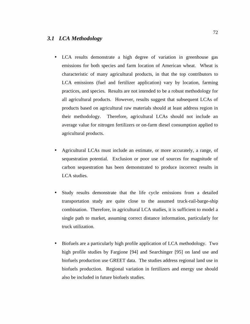
72
72
3.1 LCA Methodology
• LCA results demonstrate a high degree of variation in greenhouse gas
emissions for both species and farm location of American wheat. Wheat is
characteristic of many agricultural products, in that the top contributors to
LCA emissions (fuel and fertilizer application) vary by location, farming
practices, and species. Results are not intended to be a robust methodology for
all agricultural products. However, results suggest that subsequent LCAs of
products based on agricultural raw materials should at least address region in
their methodology. Therefore, agricultural LCAs should not include an
average value for nitrogen fertilizers or on-farm diesel consumption applied to
agricultural products.
• Agricultural LCAs must include an estimate, or more accurately, a range, of
sequestration potential. Exclusion or poor use of sources for magnitude of
carbon sequestration has been demonstrated to produce incorrect results in
LCA studies.
• Study results demonstrate that the life cycle emissions from a detailed
transportation study are quite close to the assumed truck-rail-barge-ship
combination. Therefore, in agricultural LCA studies, it is sufficient to model a
single path to market, assuming correct distance information, particularly for
truck utilization.
• Biofuels are a particularly high profile application of LCA methodology. Two
high profile studies by Fargione [94] and Searchinger [95] on land use and
biofuels production use GREET data. The studies address regional land use in
biofuels production. Regional variation in fertilizers and energy use should
also be included in future biofuels studies.

73
73
3.2 Wheat Production and Transport
• Due to the longevity of the grain industry and supporting rail infrastructure,
truck distances in the grain industry are both currently and historically low.
Agricultural rail spurs that feed major Class I main lines allow storage
facilities such low truck utilization. As rail track ages, there is increased
pressure for state governments to step in and support spur maintenance. There
are certainly many economic and rural development concerns with funding rail
spurs. However, trucks have an order of magnitude greater life cycle
emissions than either rail or barge and supporting rail spurs would maintain
low truck distances. Results would be different if short line railroad
infrastructure was not maintained.
• Nitrogen fertilizer application and on farm diesel fuel consumption were the
largest life cycle production emission contributors. This is not a study of soil
science or agricultural methods. Therefore, it is difficult to suggest reduced
tillage agriculture as a way to decrease greenhouse gas emissions. However,
since reduced tillage primarily addresses fertilizer application and fuel use,
these methods for reducing greenhouse gas emissions associated with
production would agree with study results. Reduced tillage has also been show
to have higher rates of carbon sequestration.
3.3 Future Work
• The LCA community would benefit from a regional knowledge of other large
crops, dairy farms, and meat products. Future studies would show if there’s
similar regional variation in other agricultural product classes to the variation
demonstrated for American wheat.

74
74
• The results of this study support the need for dynamic modeling in LCA. The
case study of American wheat modeled current wheat production. Ideally, a
dynamic LCA methodology would include trends in agricultural supply chain.
If a shift in modal utilization occurs, particularly trucks, this should be
modeled against currently reliance on short distance rail spurs. Similarly,
shipping grain in containers is currently economically viable only for
specialized grains. If this changes, future work should include container
movement and disposal in LCA studies.
• However, above all, consensus is needed for sequestration potential of
agricultural fields. A robust estimate will allow for more accurate agricultural
LCA studies and data at a similar resolution to energy and fertilizers use
currently collected by the USDA

75
75
References [1]Cooper, J.S. (2003): Life Cycle Assessment and Sustainable Development
Indicators. Journal of Industrial Ecology 7, 12-15
[2]Cooper, J.S., Fava J. (1999): Teaching Life-Cycle Assessment at Universities in North America. Journal of Industrial Ecology 3, 13-17
[3]Klüppel, H.J. (1998): ISO 14041: Environmental management–Life Cycle Assessment–Goal and Scope Definition–Inventory Analysis. Int J LCA 3, 301
[4]Hayashi, K., Gaillard G., Nemecek T. (2005): Life cycle assessment of agricultural production systems: current issues and future perspectives. International Seminar on Technology Development for Good Agriculture Practice in Asia and Oceania, Epochal Tsukuba
[5]Pimentel, D., Patzek T.W. (2005): Ethanol Production Using Corn, Switchgrass, and Wood; Biodiesel Production Using Soybean and Sunflower. Natural Resources Research 14, 65-76
[6]Farrell, A.E., Plevin R.J., Turner B.T., Jones A.D., O'Hare M., Kammen D.M. (2006): Ethanol Can Contribute to Energy and Environmental Goals. American Association for the Advancement of Science, pp. 506-508
[7]Hammerschlag, R. (2006): Ethanol's Energy Return on Investment: A Survey of the Literature 1990-Present. Environ. Sci. Technol 40, 1744-1750
[8]Kim, S., Dale B.E. (2005): Environmental aspects of ethanol derived from no-tilled corn grain: nonrenewable energy consumption and greenhouse gas emissions. Biomass and Bioenergy 28, 475-489
[9]Gribben, C., Gitsham M. (2007): Food Labelling: Understanding Consumer Attitudes and Behaviour. Ashridge Report
[10]Miliband, D. (Feb 27, 2007): U.K Environment Secretary. National Farmers' Union (NFU) annual conference in Birmingham

76
76
[11]Kanda, Y., Lee B.W. (2003): Japanese and Korean Corporate Sustainability Management-A Comparative Study based on Questionnaire Survey Results. IGES Kansai Research Center Discussion Paper No.3E 2003.12
[12]Bhan, N. (2007): Ecodesign, Ecolabels and the Environment: How Europe is redesigning our footprint on earth. Core77 Accessed at: http://www.core77.com/reactor/08.07_ecodesign.asp
[13]Morgan D, Born B, Cook R, Radenovic H, Renzi S (2007): Seattle Food System Enhancement Project: Greenhouse Gas Emissions Study. City of Seattle Department of Neighborhoods
[14]Narayanaswamy, V., Altham J., Van Berkel R., McGregor M. (2003): Methodological Framework for Application of Environmental Life Cycle Assessment (LCA) to Australian Grains. Curtin University of Technology, Perth, Western Australia
[15]Piringer, G., Steinberg L.J. (2006): Reevaluation of Energy Use in Wheat Production in the United States. J Ind Ecol 10
[16]Elbehri, A. (2007): The Changing Face of the U.S. Grain System. Economic Research Service, U.S. Department of Agriculture
[17]National Agricultural Statistics Service (2005): Agricultural Chemical Usage 2004 Field Crops Summary, U.S. Department of Agriculture.
[18]Tilman, D., Fargione J., Wolff B., D'Antonio C., Dobson A., Howarth R., Schindler D., Schlesinger W.H., Simberloff D., Swackhamer D. (2001): Forecasting Agriculturally Driven Global Environmental Change. Science 292, 281 - 284
[19]Tilman, D. (1999): Colloquium Paper Global environmental impacts of agricultural expansion: The need for sustainable and efficient practices. Proc Natl Acad Sci US A 96, 5995-6000
[20]Fernandez-Cornejo, J., Jans S. (1999): Pest Management in US Agriculture. US Dept. of Agriculture, Economic Research Service

77
77
[21]Halvorson, A.D., Black A.L., Krupinsky J.M., Merrill S.D., Wienhold B.J., Tanaka D.L. (2000): Spring Wheat Response to Tillage and Nitrogen Fertilization in Rotation with Sunflower and Winter Wheat. Agronomy Journal 92, 136
[22]Economic Research Service (2004): Energy Use on Major Field Crops in Surveyed States, U.S. Department of Agriculture
[23]Energy Information Administration (2007): State Electricity Profiles 2005, Office of Coal, Nuclear, Electric and Alternate Fuels
[24]Wang, L., Molburg (2004): Allocation of Energy Use in Petroleum Refineries to Petroleum Products: Implications for Life Cycle Energy Use and Emissions Inventory of Petroleum Transportation Fuels. International Journal of Life Cycle Assessment, 9 (1) 34- 44
[25]National Agricultural Statistics Service (2006): Small Grains 2006 Summary, U.S. Department of Agriculture.
[26]Eswaran, H., Vandenberg, E., Reich, P., 1993. Organic carbon soils of the world. Soil Sci. Soc. Am. J. 57, 192–194.
.
[27]Raich, J.W., Tufekcioglu, A., (2000): Vegetation and soil respiratio correlations and controls. Biogeochemistry 48, 71–90.
.
[28]Curtin, D., Wang H., Selles F., McConkey B.G., Campbell C.A. (2000): Tillage Effects on Carbon Fluxes in Continuous Wheat and Fallow-Wheat Rotations. Soil Science Society of America Journal 64, 2080
[29]Jacinthe, P.A., Lal R., Kimble J.M. (2002): Carbon budget and seasonal carbon dioxide emission from a central Ohio Luvisol as influenced by wheat residue amendment. Soil & Tillage Research 67, 147-157
[30]Yakov Kuzyakov, G.D. (2000): Carbon input by plants into the soil. Review. Journal of Plant Nutrition and Soil Science 163, 421-431

78
78
[31]Sherrod, L.A., Peterson G.A., Westfall D.G., Ahuja L.R. (2005): Soil Organic Carbon Pools After 12 Years in No-Till Dryland Agroecosystems. Soil Science Society of America Journal 69, 1600
[32]Hao, Y., Lal R., Owens L.B., Izaurralde R.C., Post W.M., Hothem D.L. (2002): Effect of cropland management and slope position on soil organic carbon pool at the North Appalachian Experimental Watersheds. Soil & Tillage Research 68, 133-142
[33]Follett, R.F. (2001): Soil management concepts and carbon sequestration in cropland soils. Soil & Tillage Research 61, 77-92
[34]Kessavalou, A., Mosier A.R., Doran J.W., Drijber R.A., Lyon D.J., Heinemeyer O. (1998): Fluxes of Carbon Dioxide, Nitrous Oxide, and Methane in Grass Sod and Winter Wheat-Fallow Tillage Management. Journal of Environmental Quality 27, 1094
[35]Purakayastha, T.J., Huggins D.R., Smith J.L. (2005): Carbon Sequestration in Native Prairie, Perennial Grass, No-Till, and Cultivated Palouse Silt Loam Soil Sci. Soc. Am. J. 72:534–540
[36]Economic Research Service (2008): State Fact Sheets. United States Departement of Agriculture (USDA).
[37]Transportation Services Branch (2006): Transportation of U.S. Grains A Modal Share Analysis, 1978-2004, U.S. Department of Agriculture Transportation and Marketing Programs
[38]Pike, Q.D., Jessup E.L., Casavant K. (2004): Washington Warehouse/distribution Center Industry Operations & Transportation Usage. Washington State University
[39]International Standards Association (2006): ISO 14040:2006, Environmental management – Life cycle assessment – Principles and framework
[40]International Standards Association (2006): ISO 14044:2006, Environmental management – Life cycle assessment – Requirements and guidelines.

79
79
[41]Heijungs, R., Suh S. (2002): The Computational Structure of Life Cycle Assessment. Kluwer Academic Publishers
[42]Cooper, J. (2008): The refined model for The refined model for inventory analysis Lecture Notes for ME599JC Life Cycle Assessment University of Washington
[43]Food and Agriculture Organization Corporate Statistical Database (FAOSTAT) (2006): ProdSTAT Summary, Food and Agriculture Organization of the United Nations, retrieved Jan 12, 2007 from http://faostat.fao.org/.
[44]National Agricultural Statistics Service (1997): United States Crop Rankings - 1997 Production Year, United States Department of Agriculture
.
[45]Bonjean, A.P., Angus W.J. (2001): The World Wheat Book: A History of Wheat Breeding. Intercept
[46]Washington Wheat Comission (2006): Washington Wheat Facts, Spokane, WA.
[47]Khoo, H., Reginald T. (2004): Report for ASEAN Biomass Meeting. Association of South East Asian Nataion (ASEAN) Biomass Meeting AIST, Tsukuba, JAPAN
[48]Lechon, Y., Cabal H., Saez R. (2005): Life cycle analysis of wheat and barley crops for bioethanol production in Spain. International Journal of Agricultural Resources, Governance and Ecology 4, 113-122
[49]Narayanaswamy, V., Altham J., Van Berkel R. (2004): Environmental Life Cycle Assessment (LCA) Case Studies for Western Australian Grain Products. Curtin University of Technology, Perth, Western Australia
[50]Koga, N., Tsuruta H., Tsuji H., Nakano H. (2003): Fuel consumption-derived CO2 emissions under conventional and reduced tillage cropping systems in northern Japan. Agriculture, Ecosystems & Environment 99, 213-219
[51]Calderini, D.F., Slafer G.A. (1998): Changes in yield and yield stability in wheat during the 20th century. Field Crops Research 57, 335-347

80
80
[52]Nemecek, T. (2006): Wheat Grains IP. at Farm, Swiss Centre for Life Cycle Inventories ECOINVENT Database.
[53]Commodities and Trade Division (2005): Policies for Basic Food Commodities: 2003-2004, Food and Agriculture Organization of the United Nations
[54]Agriculture and Agri-Food Canada (2007): Durum Wheat: 2007-2008 Situation and Outlook, Bi-weekly Bulletin, Volume 20 Number 18
.
[55]Hertwich, E., Briceno T., Hofstetter P., Inaba A. Consumption: The Contribution. Reports and Working Papers from Norwegian University of Science and Technology
(NTNU) Industrial Ecology Programme (IndEcol) Report no. 1/2005
[56]International Standards Association (1998): ISO14041: Environmental Management – LCA – Goal and scope definition and inventory analysis.
[57]Cooper, J., Nechodom M., Schuetzle D., Tamblyn G. (2006): Life Cycle Assessment of Producing Electricity from Forest Wildfire Fuels Treatments: Goal and Scope Definition for Select Environmental Impacts. Document prepared for the California Energy Emission and the US Forest Service
[58]Taylor, B. (1995): Guide for the Use of the International System of Units (SI). National Institute of Standards and Technology (NIST) Special Publications
[59]Wang, M (2005): The Greenhouse Gases, Regulated Emissions, and Energy Use in Transportation (GREET) Model: Version 1.6, Argonne National Laboratory: Argonne (unit process data extracted prior to final software results), www.transportation.anl.gov/software/GREET/.
[60]Jørgensen, A.M., Ywema, P.E., Frees, N., Exner, S., Bracke, R., (1996): Transportation in LCA: A Comparative Evaluation of the Importance of Transport in Four LCAs, International Journal of LCA 1 (4) 218-220.

81
81
[61]He, D., M. Wang (2000): Contribution of Feedstock and Fuel Transportation to Total Fuel-Cycle Energy Use and Emissions, 2000 Society of Automotive Engineers, SAE 2000-01-2976
.
[62]Clark, M.L., Jessup E.L., Casavant K., Strategic Freight Transportation A. (2003): Dynamics of Wheat and Barley Shipments on Haul Roads to and from Grain Warehouses in Washington State. Washington State University
[63]Tolliver, D., Berwick M., Kimberly V. (2005): Farm-to-Market Transportation Patterns and Truck Use in the Northern Plains. Upper Great Plains Transportation Institute
[64]Vachal, K., Reichert H., Van Wechel T. (2004): US Containerized Grain and Oilseed Exports: Industry Survey. Transportation Research Record 1873, 120-125
[65]Hill, J. (2007): Email communication. USDA's Transportation Services Branch (TSB). July 10, 2007.
[66]Commonwealth Business Media Inc., (2007): Cereal Boxes - Cream of the Crop. The Journal of Commerce. November 21, 2007.
[67]Research and Innovative Technology Administration (2007): National Transportation Atlas Database, U.S. Department of Transportation.
[68]Woods, L (2006): Modeling the Transport of Raw Materials in Life Cycle Assessment, thesis in partial fulfillment of the requirements for the degree of Master of Science. University of Washington: Seattle.
[69]Cooper, J.S., L. Woods, S.J. Lee (2008) " Distance and backhaul in commodity transport modeling " Accepted: International Journal of Life Cycle Assessment.
[70]Ugles, H. (2008): Personal Communication. President International Longshore and Warehouse Union Local 19. Jan 17, 2008.
[71]Agnew, B. (2008): Personal Communication. Cascadia Program Director. Feb 7, 2008.

82
82
[72]DRI-WEFA. (2003): Waterborne Bulk Cargo Forecast Update. The San Francisco Bay Conservation and Development Commission.
[73]Ali, M.B., Brooks N.L., McElroy R.G. (2000): Characteristics of U.S. Wheat Farming: A Snapshot. Economic Research Service, U.S. Department of Agriculture No. (SB968) 68 pp
[74]Gregory, P.J., Atwell B.J. (1991): The fate of carbon in pulse-labelled crops of barley and wheat. Plant and Soil 136, 205-213
[75]Martin, J.K., Puckridge D.W. (1982): Carbon flow through the rhizosphere of wheat crops in South Australia. The Cycling of Carbon, Nitrogen, Sulphur and Phosphorus in Terrestrial and Aquatic Ecosystems. Australian Academy of Science, Canberra, 77-81
[76]Keith, H., Oades J.M., Martin J.K. (1986): Input of carbon to soil from wheat plants. Soil biology & biochemistry 18, 445-449
[77]Martin, J.K., Merckx R. (1992): The partitioning of photosynthetically fixed carbon within the rhizosphere of mature wheat. Soil Biology and Biochemistry 24, 1147-1156
[78]Swinnen, J., Van Veen J.A., Merckx R. (1995): Carbon fluxes in the rhizosphere of winter wheat and spring barley with conventional vs integrated farming. Soil Biology and Biochemistry 27, 811-820
[79]Whipps, J.M. (1990): Carbon economy. The Rhizosphere, 59-97
[80]Majumder, B., Mandal B., Bandyopadhyay P.K., Gangopadhyay A., Mani P.K., Kundu A.L., Mazumdar D. (2008): Organic Amendments Influence Soil Organic Carbon Pools and Rice-Wheat Productivity. Soil Science Society of America Journal 72, 775
[81]Johnen, B.G., Sauerbeck D.R. (1977): A tracer technique for measuring growth, mass and microbial breakdown of plant roots during vegetation. Soil Organisms as Components of Ecosystems. Ecological Bulletins, Stockholm 25, 366-373

83
83
[82]IPCC, W.G.I. (2007): Changes in Atmospheric Constituents and in Radiative Forcing IPCC WGI 4th Assessment Report, Intergovernmental Panel on Climate Change, Geneva, 129-234
[83]Weiland, R., Smith D. (2007): Ag Decision Maker -- Metric Conversions. Iowa State University Extension File C6-80
[84]Cooper, J., Godwin C., Hall E. (2008): Modeling Process and Material Alternatives in Life Cycle Assessments. International Journal of Life Cycle Assessment 13 (2) 115-123
[85]Bureau of Transportation Statistics (2002): The 2002 Commodity Flow Survey (CFS). U.S. Department of Transportation (US DOT).
[86]Monson, J.W., Jessup E.L., Casavant K. (2005): Washington State Grain Cooperatives: History, Functions, and Regulations SFTA Research Report #16 Washington State University
[87]Lewis, E.A. (1996): American Shortline Railway Guide: Facts, Figures, and Locomotive Rosters for over 500 Short Lines (Railroad Reference Series , No 17). Kalmbach Books
[88]Washington State Transportation Commission (2006): Statewide Rail Capacity and Needs Study. May 2006.
[89]Frank, A.B., Dugas W.A. (2001): Carbon dioxide fluxes over a northern, semiarid, mixed-grass prairie. Agricultural and Forest Meteorology 108, 317-326
[90]Food and Agriculture Organization of the United Nations (2004): Carbon sequestration in dryland soils. World Soils Resources Reports 102. Rome.
[91]Nemecek, T., Heil A., Huguenin O., Meier S. (2004): Life Cycle Inventories of Agricultural Production Systems. ecoinvent report No. 15
[92]Smith, P., Goulding, K.W., Smith, K.A., Powlson, D.S., Smith, J.U., Falloon, P. & , Coleman K. (2001): Enhancing the carbon sink in European agricultural soils:

84
84
including trace gas fluxes in estimates of carbon mitigation potential. Nut. Cyc. Agroeco 60: 237–252
[93]Metting, F., Smith, J. & Amthor, J. (1999): Science needs and new technology for soil carbon sequestration in soils: Science monitoring and beyond. Proc. St. Michaels Workshop Columbus, USA, Battelle Press, pp 1–34
[94]Fargione, J., Hill J., Tilman D., Polasky S., Hawthorne P. (2008): Land Clearing and the Biofuel Carbon Debt. Science 319, 1235-1238
[95]Searchinger, T., Heimlich R., Houghton R.A., Dong F., Elobeid A., Fabiosa J., Tokgoz S., Hayes D., Yu T.-H. (2008): Use of U.S. Croplands for Biofuels Increases Greenhouse Gases Through Emissions from Land-Use Change. Science 319, 1238-1240

85
Appendix A: U.S. Wheat Yield By State and Species Data for wheat yield by state and species was extracted from the U.S. Department of Agriculture’s 2006 Small Grains Summary [25]. Significant figures are unmodified.
Spring Wheat Hard Red Hard White Soft White 2005 2006 2005 2006 2005 2006
STATE 1,000 Bushels
1,000 Bushels Average Percent
1,000 Bushels
1,000 Bushels Average Percent
1,000 Bushels
1,000 Bushels
CO 963 1211 1087 0% 0 32 16 0% 272 371 ID 11988 19214 15601 3% 2592 3431 3012 56% 17820 11665 MN 70930 77550 74240 17% 0 0 0 0% 0 0 MT 80784 63162 71973 16% 816 638 727 14% 0 0 NV 26 9 17 0% 0 0 0 0% 230 167 ND 224400 212350 218375 49% 0 0 0 0% 0 0 OR 1136 2588 1862 0% 0 0 0 0% 4844 3163 SD 67600 42600 55100 12% 0 0 0 0% 0 0 UT 498 327 412 0% 0 0 0 0% 256 168 WA 7667 12750 10209 2% 1122 2125 1624 30% 9911 6375 WI 287 350 319 0% 0 0 0 0% 0 0 WY 309 229 269 0% 0 0 0 0% 6 5 466587 432339 449463 4530 6226 5378

86
Winter Wheat
Hard Red Soft Red Hard White
2005 2006 2005 2006 2005 2006
STATE 1,000 Bushels
1,000 Bushels Average Percent
1,000 Bushels
1,000 Bushels Average Percent
1,000 Bushels
1,000 Bushels
AL 0 0 0 0% 2250 2610 2430 1% 0 0 0 0% AZ 160 180 170 0% 0 0 0 0% 0 0 0 0% AR 0 0 0 0% 8320 18605 13463 4% 0 0 0 0% CA 19008 12035 15522 2% 0 0 0 0% 648 1015 832 4% CO 48576 37107 42842 5% 0 0 0 0% 4224 2793 3509 18% DE 0 0 0 0% 3570 3015 3293 1% 0 0 0 0% FL 0 0 0 0% 360 210 285 0% 0 0 0 0% GA 0 0 0 0% 7280 5880 6580 2% 0 0 0 0% ID 11293 10934 11114 1% 0 0 0 0% 664 547 606 3% IL 366 1219 793 0% 36234 59751 47992 14% 0 0 0 0% IN 0 0 0 0% 24480 31740 28110 8% 0 0 0 0% IA 450 653 552 0% 300 535 417 0% 0 0 0 0% KS 364800 285376 325088 41% 0 0 0 0% 15200 5824 10512 55% KY 612 227 420 0% 19788 22493 21140 6% 0 0 0 0% LA 144 167 155 0% 4656 5398 5027 1% 0 0 0 0% MD 0 0 0 0% 9240 8500 8870 3% 0 0 0 0% MI 779 1424 1101 0% 22585 28945 25765 7% 0 0 0 0% MN 540 2790 1665 0% 0 0 0 0% 0 0 0 0% MS 0 0 0 0% 3250 4307 3779 1% 0 0 0 0% MO 1750 2948 2349 0% 27410 46192 36801 11% 0 0 0 0% MT 92610 80909 86759 11% 0 0 0 0% 1890 1651 1771 9% NE 67267 60588 63928 8% 0 0 0 0% 1373 612 992 5% NV 0 0 0 0% 0 0 0 0% 0 26 13 0% NJ 0 0 0 0% 1219 1320 1270 0% 0 0 0 0% NM 9720 3840 6780 1% 0 0 0 0% 0 0 0 0% NY 103 174 138 0% 1488 1970 1729 0% 0 0 0 0%
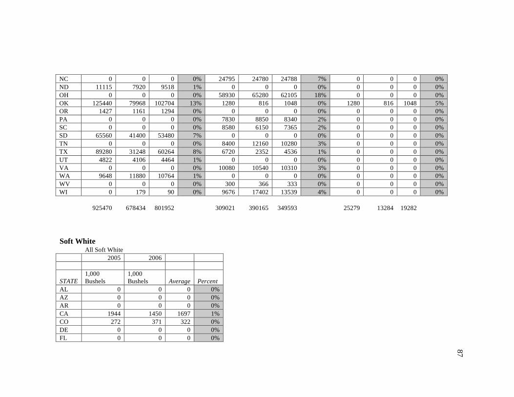
87
NC 0 0 0 0% 24795 24780 24788 7% 0 0 0 0% ND 11115 7920 9518 1% 0 0 0 0% 0 0 0 0% OH 0 0 0 0% 58930 65280 62105 18% 0 0 0 0% OK 125440 79968 102704 13% 1280 816 1048 0% 1280 816 1048 5% OR 1427 1161 1294 0% 0 0 0 0% 0 0 0 0% PA 0 0 0 0% 7830 8850 8340 2% 0 0 0 0% SC 0 0 0 0% 8580 6150 7365 2% 0 0 0 0% SD 65560 41400 53480 7% 0 0 0 0% 0 0 0 0% TN 0 0 0 0% 8400 12160 10280 3% 0 0 0 0% TX 89280 31248 60264 8% 6720 2352 4536 1% 0 0 0 0% UT 4822 4106 4464 1% 0 0 0 0% 0 0 0 0% VA 0 0 0 0% 10080 10540 10310 3% 0 0 0 0% WA 9648 11880 10764 1% 0 0 0 0% 0 0 0 0% WV 0 0 0 0% 300 366 333 0% 0 0 0 0% WI 0 179 90 0% 9676 17402 13539 4% 0 0 0 0% 925470 678434 801952 309021 390165 349593 25279 13284 19282
Soft White All Soft White 2005 2006
STATE 1,000 Bushels
1,000 Bushels Average Percent
AL 0 0 0 0% AZ 0 0 0 0% AR 0 0 0 0% CA 1944 1450 1697 1% CO 272 371 322 0% DE 0 0 0 0% FL 0 0 0 0%

88
GA 0 0 0 0% ID 72293 54855 63574 25% IL 0 0 0 0% IN 0 0 0 0% IA 0 0 0 0% KS 0 0 0 0% KY 0 0 0 0% LA 0 0 0 0% MD 0 0 0 0% MI 15576 17082 16329 6% MN 0 0 0 0% MS 0 0 0 0% MO 0 0 0 0% MT 0 0 0 0% NE 0 0 0 0% NV 780 1021 900 0% NJ 0 0 0 0% NM 0 0 0 0% NY 3540 3651 3595 1% NC 0 0 0 0% ND 0 0 0 0% OH 0 0 0 0% OK 0 0 0 0% OR 50996 40692 45844 18% UT 1779 1687 1733 1% VA 0 0 0 0% WA 120863 113295 117079 47% WV 0 0 0 0% WI 299 359 329 0% 268342 234462 251402

89
89
Appendix B: Chemical Application Extraction from Agricultural Chemical Usage Summary [17]. Significant figures are unmodified.
The agricultural chemical use estimates in this report refer to on-farm use of commercial fertilizers and pesticides on targeted crops for the 2004 crop year. Targeted crops included durum wheat, peanuts, soybeans, other spring wheat, and winter wheat. Farm and ranch operators were enumerated late in the growing season after the farm operator had indicated that planned applications were completed. The chemical use data were not summarized for geographical areas other than those States published in this report.
The data were compiled from two surveys, the Agricultural Resources Management Survey (ARMS) and Conservation Effects Assessment Project (CEAP). Data collection occurred primarily during the months of September to December of 2004. This report excludes pesticides used for seed treatments and post harvest applications to the commodity. The table below shows the number of States surveyed, the number of summarized reports for each State, and the percent of the Program States’ acres planted to that commodity compared with the U.S. total.

90
90
Spring Wheat Fertilizer Application
Primary Planted Area Appli- Rate per Rate per Total Nutrient Acreage Applied cations Application Crop Year Applied
1,000 Acres Percent Number Pounds per Acre
Pounds per Acre
Mil. lbs
Idaho 500 Nitrogen 93 1.7 71 121 56.1
Phosphate 63 1.2 33 41 12.7
Potash 23 1.2 30 37 4.4
Minnesota 1,700 Nitrogen 98 1.6 67 108 180.1
Phosphate 91 1.1 43 49 75.5
Potash 54 1.2 32 38 34.8
Montana 3,000 Nitrogen 79 1.7 34 57 134.6
Phosphate 69 1.3 26 35 72.6
Potash 13 1.4 16 22 9
North Dakota 6,200 Nitrogen 98 2.5 46 114 691.9
Phosphate 86 1.6 32 50 269
Potash 27 1.5 16 24 39.9
Oregon 180 Nitrogen 91 1.2 50 59 9.7
Phosphate 28 1.1 32 34 1.7
Potash 9 1 33 34 0.5
South Dakota 1,600 Nitrogen 92 1.7 54 90 132.5
Phosphate 68 1.2 40 49 53.2
Potash 19 1.3 22 28 8.5
Washington 530 Nitrogen 100 1.4 59 86 45.4
Phosphate 67 1.2 17 21 7.4
Potash 9 1.1 38 43 2.1
Total 13,710 Nitrogen 93 2 48 98 1,250.30
Phosphate 79 1.4 33 46 492.1
Potash 25 1.4 21 29 99.2

91
91
Active Area Appli- Rate per Rate per Total
Ingredient Applied cations Application Crop Year Applied
Percent Number Pounds per Acre
Pounds per Acre 1,000 lbs
Herbicides 2,4-D 20 1.1 0.35 0.39 1,076
2,4-D, Dimeth. salt 1 1 0.19 0.19 39 2,4-DP, Dimeth. salt 4 1 0.41 0.41 212 Acetic acid (2,4-D) 8 1 0.27 0.27 297 Bromoxynil 16 1 0.24 0.24 515 Bromoxynil octanoate 19 1 0.25 0.25 647
Butoxy. ester 2,4-D Carfentrazone-ethyl Chlorsulfuron
2 * * 1.0 1.0 1.0 0.39 0.006 0.01
0.40 0.006 0.01
134 ( 2 ) ( 2 )
Clodinafop-propargil 14 1 0.06 0.06 106 Clopyralid 6 1 0.07 0.07 60 Dicamba 11 1.1 0.08 0.09 135 Dicamba, Sodium salt 1 1 0.08 0.08 8
Fenoxaprop 31 1 0.06 0.06 270
Flucarbazone-sodium 7 1 0.02 0.02 17
Fluroxypyr 8 1 0.08 0.08 89
Fluroxypyr 1-methylh 6 1 0.09 0.09 75
Glyphosate 23 1.1 0.44 0.49 1,555
Imazamethabenz * 1 0.1 0.1 4
MCPA 46 1 0.29 0.29 1,845
MCPA, dimethyl. salt 2 1 0.42 0.42 107
MCPA-EHE 3 1 0.29 0.29 105
Metsulfuron-methyl 5 1 0.003 0.003 2
Picloram * 1 0.02 0.02 1
Prosulfuron 1 1 0.01 0.01 1
Thifensulfuron 16 1 0.009 0.009 19
Tribenuron-methyl 14 1 0.006 0.006 12
Trifluralin 1 1 0.33 0.33 49
Insecticides Chlorpyrifos * 1 0.3 0.3 9
Dimethoate * 1 0.27 0.27 7
Zeta-cypermethrin * 1 0.02 0.02 -2
Fungicides Propiconazole 9 1 0.07 0.07 87
Pyraclostrobin 6 1 0.06 0.06 48
Tebuconazole 12 1 0.1 0.1 162

92
92
Winter Wheat Fertilizer Application
Primary Planted Area Appli- Rate per Rate per Total Nutrient Acreage Applied cations Application Crop
Year Applied
1,000 Acres Percent Number Pounds per Acre
Pounds per Acre
Mil. lbs
Colorado 2,300 Nitrogen 59 1.4 27 38 51.2
Phosphate 31 1.3 17 23 15.8
Potash 5 1.1 24 25 2.7
Idaho 750
Nitrogen 89 2 68 134 89.2 Phosphate 62 1.4 29 40 18.5
Potash 31 1.5 18 26 6.1
Illinois 920
Nitrogen 98 2.1 55 115 103.2 Phosphate 85 1.3 75 94 74.2
Potash 77 1.3 104 130 92.3
Kansas 10,000 Nitrogen 90 2.2 39 87 788.6
Phosphate 62 1.5 29 45 281.8
Potash 6 1.4 26 37 23.4
Michigan 660 Nitrogen 97 2.2 53 115 73.5
Phosphate 71 1.2 50 59 27.5
Potash 77 1.2 64 75 38.4
Missouri 1,050 Nitrogen 97 2 61 124 125.9
Phosphate 84 1.2 50 60 52.9
Potash 86 1.2 66 78 70
Montana 1,900 Nitrogen 92 1.6 30 47 83
Phosphate 83 1.1 28 30 47.3
Potash 21 1.1 9 10 3.9
Nebraska 1,850 Nitrogen 73 1.8 32 57 76.4
Phosphate 42 1.2 26 31 24.3
Potash 3 1.7 13 22 1.2
Ohio 920

93
93
Nitrogen 100 2.2 44 100 91.6 Phosphate 95 1.1 66 75 65.8
Potash 90 1.2 72 84 69.5
Oklahoma 6,200 Nitrogen 92 2.3 44 100 571
Phosphate 62 1.5 26 39 147.8
Potash 13 1.4 19 26 22
Oregon 820 Nitrogen 96 1.4 57 82 64.7
Phosphate 11 1.6 35 57 5.3
Potash 6 1.3 38 50 2.5
South Dakota 1,650 Nitrogen 77 1.6 51 83 105.8
Phosphate 58 1.2 38 47 44.6
Potash 7 1.3 33 43 5.1
Texas 6,300 Nitrogen 64 1.8 47 86 347.7
Phosphate 35 1.4 37 53 116.6
Potash 9 1.1 15 17 9.6
Washington 1,800 Nitrogen 97 1.5 61 93 161.2
Phosphate 24 1.6 18 27 11.6
Potash 3 1.6 17 28 1.4
Total 37,120 Nitrogen 84 2 44 88 2,733.00
Phosphate 55 1.4 33 46 934
Potash 16 1.2 47 58 348.1

94
94
Active Area Appli- Rate per Rate per Total Ingredient Applied cations Application Crop Year Applied
Percent Number Pounds per
Acre Pounds per Acre 1,000 lbs
Herbicides 2,4-D 13 1.4 0.33 0.45 2,173 2,4-D, Dimeth. salt
1 1.2 0.27 0.32 144
2,4-DP, Dimeth. salt
5 1.3 0.34 0.45 786
Acetamide * 1 0.34 0.34 9
Acetic acid (2,4-D) 1 1.1 0.29 0.32 145 Atrazine 1 1.4 0.54 0.73 223
Bromoxynil 2 1 0.27 0.28 154 Bromoxynil octanoate
1 1 0.24 0.24 105
Butoxy. ester 2,4-D
2 1.1 0.53 0.57 352
Carfentrazone-ethyl
* 1 0.03 0.03 1
Chlorsulfuron 8 1 0.01 0.01 32
Clodinafop-propargil 1 1 0.04 0.04 10 Clopyralid 1 1 0.09 0.09 18
Dicamba 6 1.2 0.1 0.12 269
Diclofop-methyl * 1 0.67 0.67 89 Diuron * 1 1.1 1.1 20
Fenoxaprop * 1 0.08 0.08 3 Flucarbazone-sodium
* 1 0.02 0.02 1
Fluroxypyr 1 1 0.09 0.09 30 Fluroxypyr 1-methylh
* 1 0.1 0.1 7
Glyphosate 13 1.9 0.42 0.78 3,648 Imazamox 1 1 0.03 0.03 9
MCPA 4 1.1 0.32 0.37 498 MCPA, dimethyl. salt * 1 0.53 0.53 60 Mesosulfuron-Methyl
* 1 0.01 0.01 1
Metribuzin 1 1.7 0.27 0.46 135
Metsulfuron- 15 1.1 0.002 0.002 13

95
95
methyl Picloram 1 1 0.01 0.01 2
Prosulfuron * 1 0.02 0.02 1
Sulfosulfuron 4 1 0.03 0.03 33
Thifensulfuron 9 1.1 0.008 0.009 29
Tralkoxydim * 1 0.14 0.14 8 Triallate * 1 1.08 1.08 85
Triasulfuron 4 1.1 0.02 0.02 25 Tribenuron-methyl
10 1.1 0.004 0.004 15
Insecticides Chlorpyrifos 3 1 0.36 0.36 438 Dimethoate * 1 0.31 0.31 21
Ethyl parathion 1 1 0.63 0.63 133 Lambda-cyhalothrin
1 1 0.02 0.02 6
Zeta-cypermethrin
1 1 0.03 0.03 10
Fungicides Azoxystrobin * 1 0.07 0.07 13
Propiconazole 1 1 0.1 0.1 35
Pyraclostrobin 1 1.1 0.09 0.1 22
Tebuconazole 1 1 0.04 0.04 15
Trifloxystrobin * 1.2 0.07 0.08 2

96
Appendix C: Energy Use Estimates of State-average fuel consumption from surveys of crop producers during 1997 to 2002 are presented here and extracted from the U.S. Department of Agriculture’s Energy Use on Major Field Crops in Surveyed States [22]. Significant figures are unmodified.

97

98

99
Appendix D: Inventory Results for Wheat Production
MONTANA - Hard Red Winter
YIELD 4.30E+01 Bushels/acre
Process Input Unit
Input (normalized to yield) Unit Intensity Unit
Process Reference
CO2 Emission (gCO2 eq./kg Wheat)
Relative %
Nitrogen fertilizer (N) 5.27E+01 kg/ha 1.88E-02 kg fertilizer/kg Wheat 2.94E+00 kg CO2/kg fertilizer GREET 1.7 5.54E+01 39.0%
Phosphorous fertilizer (P2O5) 3.36E+01 kg/ha 1.20E-02 kg/kg Wheat 6.70E-01 kg CO2/kg fertilizer GREET 1.7 8.06E+00 5.7% Potassium Fertilizer (K2O) 1.12E+01 kg/ha 4.01E-03 kg/kg Wheat 9.90E-01 kg CO2/kg fertilizer GREET 1.7 3.97E+00 2.8% Limestone 4.48E+01 kg/ha 1.60E-02 kg/kg Wheat 6.10E-01 kg CO2/kg fertilizer GREET 1.7 9.78E+00 6.9%
Herbicides 2.80E-01 kg/ha 1.00E-04 kg/kg Wheat 2.08E+01 kg CO2/kg herbacide GREET 1.7 2.08E+00 1.5%
Insecticides 2.01E-02 kg/ha 7.18E-06 kg/kg Wheat 2.43E+01 kg CO2/kg insecticides GREET 1.7 1.74E-01 0.1%
Diesel!Farm machinery) 3.19E+01 L/ha 1.14E-02 L/kg Wheat 3.35E+00 kg CO2/L consumed GREET 1.7 3.82E+01 26.9% Diesel (Custom operation) 7.79E+00 L/ha 2.79E-03 L/kg Wheat 3.35E+00 kg CO2/L consumed GREET 1.7 9.34E+00 6.6%
Electricity 2.69E+01 kWh/ha 9.63E-03 kWh/kg Wheat 5.34E-01 kg CO2/kWh
GREET 1.7 (assuming local mix) 5.15E+00 3.6%
Gasoline 9.37E+00 L/ha 3.35E-03 L/kg Wheat 2.97E+00 kg CO2/L consumed GREET 1.7 9.96E+00 7.0% LP Gas 0.00E+00 L/ha 0.00E+00 L/kg Wheat 2.84E+00 kg CO2/L consumed GREET 1.7 0.00E+00 0.0%
Natural Gas 0.00E+00 m3/ha 0.00E+00 m3/kg Wheat 2.35E+00 kg CO2/m3 consumed GREET 1.7 0.00E+00 0.0%
RAW TOTAL 1.42E+02 ALLOCATION 95.5%
TOTAL 1.36E+02

100
KANSAS - Hard Red Winter
YIELD 3.60E+01 Bushels/acre
Process Input Unit Input Unit Intensity Unit Process Reference
CO2 Emission (g-CO2/kg Wheat) %
Nitrogen fertilizer (N) 9.75E+01 kg/ha 4.17E-02 kg fertilizer/kg Wheat 2.94E+00 kg CO2/kg fertilizer GREET 1.7 1.22E+02 46.6%
Phosphorous fertilizer (P2O5) 5.04E+01 kg/ha 2.16E-02 kg/kg Wheat 6.70E-01 kg CO2/kg fertilizer GREET 1.7 1.44E+01 5.5% Potassium Fertilizer (K2O) 4.15E+01 kg/ha 1.77E-02 kg/kg Wheat 9.90E-01 kg CO2/kg fertilizer GREET 1.7 1.75E+01 6.7% Limestone 4.48E+01 kg/ha 1.92E-02 kg/kg Wheat 6.10E-01 kg CO2/kg fertilizer GREET 1.7 1.17E+01 4.4% Herbicides 2.80E-01 kg/ha 1.19E-04 kg/kg Wheat 2.08E+01 kg CO2/kg herbacide GREET 1.7 2.48E+00 0.9%
Insecticides 2.25E-02 kg/ha 9.61E-06 kg/kg Wheat 2.43E+01 kg CO2/kg insecticides GREET 1.7 2.34E-01 0.1%
Diesel!Farm machinery) 4.31E+01 L/ha 1.84E-02 L/kg Wheat 3.35E+00 kg CO2/L consumed GREET 1.7 6.17E+01 23.5% Diesel (Custom operation) 7.79E+00 L/ha 3.33E-03 L/kg Wheat 3.35E+00 kg CO2/L consumed GREET 1.7 1.12E+01 4.2%
Electricity 0.00E+00 kWh/ha 0.00E+00 kWh/kg Wheat 8.36E-01 kg CO2/kWh
GREET 1.7 (assuming local mix) 0.00E+00 0.0%
Gasoline 8.43E+00 L/ha 3.60E-03 L/kg Wheat 2.97E+00 kg CO2/L consumed GREET 1.7 1.07E+01 4.1% LP Gas 8.43E+00 L/ha 3.60E-03 L/kg Wheat 2.84E+00 kg CO2/L consumed GREET 1.7 1.02E+01 3.9%
Natural Gas 1.40E-02 m3/ha 5.98E-06 m3/kg Wheat 2.35E+00 kg CO2/m3 consumed GREET 1.7 1.40E-02 0.0%
RAW TOTAL 2.63E+02 ALLOCATION 95.5%
TOTAL 2.51E+02

101
OKLAHOMA - Hard Red Winter
YIELD 3.00E+01 Bushels/acre
Process Input Unit Input Unit Intensity Unit Process Reference
CO2 Emission (g-CO2/kg Wheat) %
Nitrogen fertilizer (N) 1.12E+02 kg/ha 5.75E-02 kg fertilizer/kg Wheat 2.94E+00 kg CO2/kg fertilizer GREET 1.7 1.69E+02 51.0%
Phosphorous fertilizer (P2O5) 4.37E+01 kg/ha 2.24E-02 kg/kg Wheat 6.70E-01 kg CO2/kg fertilizer GREET 1.7 1.50E+01 4.5% Potassium Fertilizer (K2O) 2.91E+01 kg/ha 1.49E-02 kg/kg Wheat 9.90E-01 kg CO2/kg fertilizer GREET 1.7 1.48E+01 4.5% Limestone 4.48E+01 kg/ha 2.30E-02 kg/kg Wheat 6.10E-01 kg CO2/kg fertilizer GREET 1.7 1.40E+01 4.2% Herbicides 2.80E-01 kg/ha 1.43E-04 kg/kg Wheat 2.08E+01 kg CO2/kg herbacide GREET 1.7 2.98E+00 0.9%
Insecticides 2.25E-02 kg/ha 1.15E-05 kg/kg Wheat 2.43E+01 kg CO2/kg insecticides GREET 1.7 2.80E-01 0.1%
Diesel!Farm machinery) 5.34E+01 L/ha 2.74E-02 L/kg Wheat 3.35E+00 kg CO2/L consumed GREET 1.7 9.18E+01 27.7% Diesel (Custom operation) 7.79E+00 L/ha 3.99E-03 L/kg Wheat 3.35E+00 kg CO2/L consumed GREET 1.7 1.34E+01 4.0%
Electricity 0.00E+00 kWh/ha 0.00E+00 kWh/kg Wheat 7.66E-01 kg CO2/kWh
GREET 1.7 (assuming local mix) 0.00E+00 0.0%
Gasoline 6.56E+00 L/ha 3.36E-03 L/kg Wheat 2.97E+00 kg CO2/L consumed GREET 1.7 1.00E+01 3.0% LP Gas 0.00E+00 L/ha 0.00E+00 L/kg Wheat 2.84E+00 kg CO2/L consumed GREET 1.7 0.00E+00 0.0%
Natural Gas 0.00E+00 m3/ha 0.00E+00 m3/kg Wheat 2.35E+00 kg CO2/m3 consumed GREET 1.7 0.00E+00 0.0%
RAW TOTAL 3.31E+02 ALLOCATION 95.5%
TOTAL 3.16E+02

102
MONTANA - Hard Red Spring
YIELD 2.83E+01 Bushels/acre
Process Input Unit Input Unit Intensity Unit Process Reference
CO2 Emission (g-CO2/kg Wheat) %
Nitrogen fertilizer (N) 6.39E+01 kg/ha 3.47E-02 kg fertilizer/kg Wheat 2.94E+00 kg CO2/kg fertilizer GREET 1.7 1.02E+02 41.4%
Phosphorous fertilizer (P2O5) 3.92E+01 kg/ha 2.13E-02 kg/kg Wheat 6.70E-01 kg CO2/kg fertilizer GREET 1.7 1.43E+01 5.8% Potassium Fertilizer (K2O) 2.47E+01 kg/ha 1.34E-02 kg/kg Wheat 9.90E-01 kg CO2/kg fertilizer GREET 1.7 1.33E+01 5.4% Limestone 4.48E+01 kg/ha 2.43E-02 kg/kg Wheat 6.10E-01 kg CO2/kg fertilizer GREET 1.7 1.48E+01 6.0% Herbicides 6.25E-01 kg/ha 3.39E-04 kg/kg Wheat 2.08E+01 kg CO2/kg herbacide GREET 1.7 7.06E+00 2.9%
Insecticides 4.25E-03 kg/ha 2.31E-06 kg/kg Wheat 2.43E+01 kg CO2/kg insecticides GREET 1.7 5.61E-02 0.0%
Diesel!Farm machinery) 3.19E+01 L/ha 1.73E-02 L/kg Wheat 3.35E+00 kg CO2/L consumed GREET 1.7 5.80E+01 23.5% Diesel (Custom operation) 7.79E+00 L/ha 4.23E-03 L/kg Wheat 3.35E+00 kg CO2/L consumed GREET 1.7 1.42E+01 5.8%
Electricity 2.69E+01 kWh/ha 1.46E-02 kWh/kg Wheat 5.28E-01 kg CO2/kWh
GREET 1.7 (assuming local mix) 7.72E+00 3.1%
Gasoline 9.37E+00 L/ha 5.09E-03 L/kg Wheat 2.97E+00 kg CO2/L consumed GREET 1.7 1.51E+01 6.1% LP Gas 0.00E+00 L/ha 0.00E+00 L/kg Wheat 2.84E+00 kg CO2/L consumed GREET 1.7 0.00E+00 0.0%
Natural Gas 0.00E+00 m3/ha 0.00E+00 m3/kg Wheat 2.35E+00 kg CO2/m3 consumed GREET 1.7 0.00E+00 0.0%
RAW TOTAL 2.46E+02 ALLOCATION 94.7%
TOTAL 2.33E+02

103
MINNESOTA - Hard Red Spring
YIELD 4.77E+01 Bushels/acre
Process Input Unit Input Unit Intensity Unit Process Reference
CO2 Emission (g-CO2/kg Wheat) %
Nitrogen fertilizer (N) 1.21E+02 kg/ha 3.91E-02 kg fertilizer/kg Wheat 2.94E+00 kg CO2/kg fertilizer GREET 1.7 1.15E+02 53.9%
Phosphorous fertilizer (P2O5) 5.49E+01 kg/ha 1.77E-02 kg/kg Wheat 6.70E-01 kg CO2/kg fertilizer GREET 1.7 1.19E+01 5.6% Potassium Fertilizer (K2O) 4.26E+01 kg/ha 1.37E-02 kg/kg Wheat 9.90E-01 kg CO2/kg fertilizer GREET 1.7 1.36E+01 6.4% Limestone 4.48E+01 kg/ha 1.45E-02 kg/kg Wheat 6.10E-01 kg CO2/kg fertilizer GREET 1.7 8.82E+00 4.1%
Herbicides 6.25E-01 kg/ha 2.02E-04 kg/kg Wheat 2.08E+01 kg CO2/kg herbacide GREET 1.7 4.20E+00 2.0%
Insecticides 4.25E-03 kg/ha 1.37E-06 kg/kg Wheat 2.43E+01 kg CO2/kg insecticides GREET 1.7 3.33E-02 0.0%
Diesel!Farm machinery) 3.75E+01 L/ha 1.21E-02 L/kg Wheat 3.35E+00 kg CO2/L consumed GREET 1.7 4.05E+01 19.0% Diesel (Custom operation) 7.79E+00 L/ha 2.51E-03 L/kg Wheat 3.35E+00 kg CO2/L consumed GREET 1.7 8.43E+00 4.0%
Electricity 0.00E+00 kWh/ha 0.00E+00 kWh/kg Wheat 7.70E-01 kg CO2/kWh
GREET 1.7 (assuming local mix) 0.00E+00 0.0%
Gasoline 9.37E+00 L/ha 3.02E-03 L/kg Wheat 2.97E+00 kg CO2/L consumed GREET 1.7 8.99E+00 4.2% LP Gas 1.87E+00 L/ha 6.05E-04 L/kg Wheat 2.84E+00 kg CO2/L consumed GREET 1.7 1.72E+00 0.8%
Natural Gas 0.00E+00 m3/ha 0.00E+00 m3/kg Wheat 2.35E+00 kg CO2/m3 consumed GREET 1.7 0.00E+00 0.0%
RAW TOTAL 2.13E+02 ALLOCATION 94.7%
TOTAL 2.02E+02

104
NORTH DAKOTA - Hard Red Spring
YIELD 3.53E+01 Bushels/acre
Process Input Unit Input Unit Intensity Unit Process Reference
CO2 Emission (g-CO2/kg Wheat) %
Nitrogen fertilizer (N) 1.28E+02 kg/ha 5.56E-02 kg fertilizer/kg Wheat 2.94E+00 kg CO2/kg fertilizer GREET 1.7 1.64E+02 57.0%
Phosphorous fertilizer (P2O5) 5.60E+01 kg/ha 2.44E-02 kg/kg Wheat 6.70E-01 kg CO2/kg fertilizer GREET 1.7 1.63E+01 5.7%
Potassium Fertilizer (K2O) 2.69E+01 kg/ha 1.17E-02 kg/kg Wheat 9.90E-01 kg CO2/kg fertilizer GREET 1.7 1.16E+01 4.0% Limestone 4.48E+01 kg/ha 1.95E-02 kg/kg Wheat 6.10E-01 kg CO2/kg fertilizer GREET 1.7 1.19E+01 4.1% Herbicides 6.25E-01 kg/ha 2.72E-04 kg/kg Wheat 2.08E+01 kg CO2/kg herbacide GREET 1.7 5.66E+00 2.0%
Insecticides 4.25E-03 kg/ha 1.85E-06 kg/kg Wheat 2.43E+01 kg CO2/kg insecticides GREET 1.7 4.50E-02 0.0%
Diesel!Farm machinery) 3.37E+01 L/ha 1.47E-02 L/kg Wheat 3.35E+00 kg CO2/L consumed GREET 1.7 4.92E+01 17.1% Diesel (Custom operation) 7.79E+00 L/ha 3.39E-03 L/kg Wheat 3.35E+00 kg CO2/L consumed GREET 1.7 1.14E+01 4.0%
Electricity 1.11E+01 kWh/ha 4.84E-03 kWh/kg Wheat 1.10E+00 kg CO2/kWh
GREET 1.7 (assuming local mix) 5.34E+00 1.9%
Gasoline 9.37E+00 L/ha 4.08E-03 L/kg Wheat 2.97E+00 kg CO2/L consumed GREET 1.7 1.21E+01 4.2% LP Gas 0.00E+00 L/ha 0.00E+00 L/kg Wheat 2.84E+00 kg CO2/L consumed GREET 1.7 0.00E+00 0.0%
Natural Gas 0.00E+00 m3/ha 0.00E+00 m3/kg Wheat 2.35E+00 kg CO2/m3 consumed GREET 1.7 0.00E+00 0.0%
RAW TOTAL 2.87E+02 ALLOCATION 94.7%
TOTAL 2.72E+02

105
MISSOURI - Soft Red Winter
YIELD 5.33E+01 Bushels/acre
Process Input Unit Input Unit Intensity Unit Process Reference
CO2 Emission (g-CO2/kg Wheat) %
Nitrogen fertilizer (N) 1.39E+02 kg/ha 4.01E-02 kg fertilizer/kg Wheat 2.94E+00 kg CO2/kg fertilizer GREET 1.7 1.18E+02 51.5%
Phosphorous fertilizer (P2O5) 6.73E+01 kg/ha 1.94E-02 kg/kg Wheat 6.70E-01 kg CO2/kg fertilizer GREET 1.7 1.30E+01 5.7% Potassium Fertilizer (K2O) 8.74E+01 kg/ha 2.52E-02 kg/kg Wheat 9.90E-01 kg CO2/kg fertilizer GREET 1.7 2.50E+01 10.9% Limestone 4.48E+01 kg/ha 1.29E-02 kg/kg Wheat 6.10E-01 kg CO2/kg fertilizer GREET 1.7 7.89E+00 3.4% Herbicides 2.80E-01 kg/ha 8.06E-05 kg/kg Wheat 2.08E+01 kg CO2/kg herbacide GREET 1.7 1.68E+00 0.7%
Insecticides 2.25E-02 kg/ha 6.49E-06 kg/kg Wheat 2.43E+01 kg CO2/kg insecticides GREET 1.7 1.58E-01 0.1%
Diesel!Farm machinery) 4.12E+01 L/ha 1.19E-02 L/kg Wheat 3.35E+00 kg CO2/L consumed GREET 1.7 3.99E+01 17.4% Diesel (Custom operation) 7.79E+00 L/ha 2.25E-03 L/kg Wheat 3.35E+00 kg CO2/L consumed GREET 1.7 7.53E+00 3.3%
Electricity 7.17E+00 kWh/ha 2.07E-03 kWh/kg Wheat 9.96E-01 kg CO2/kWh
GREET 1.7 (assuming local mix) 2.06E+00 0.9%
Gasoline 1.59E+01 L/ha 4.59E-03 L/kg Wheat 2.97E+00 kg CO2/L consumed GREET 1.7 1.37E+01 6.0% LP Gas 0.00E+00 L/ha 0.00E+00 L/kg Wheat 2.84E+00 kg CO2/L consumed GREET 1.7 0.00E+00 0.0%
Natural Gas 0.00E+00 m3/ha 0.00E+00 m3/kg Wheat 2.35E+00 kg CO2/m3 consumed GREET 1.7 0.00E+00 0.0%
RAW TOTAL 2.29E+02 ALLOCATION 95.6%
TOTAL 2.19E+02

106
ILLINOIS - Soft Red Winter
YIELD 6.23E+01 Bushels/acre
Process Input Unit Input Unit Intensity Unit Process Reference
CO2 Emission (g-CO2/kg Wheat) %
Nitrogen fertilizer (N) 1.29E+02 kg/ha 3.18E-02 kg fertilizer/kg Wheat 2.94E+00 kg CO2/kg fertilizer GREET 1.7 9.35E+01 49.6%
Phosphorous fertilizer (P2O5) 1.05E+02 kg/ha 2.60E-02 kg/kg Wheat 6.70E-01 kg CO2/kg fertilizer GREET 1.7 1.74E+01 9.2% Potassium Fertilizer (K2O) 1.46E+02 kg/ha 3.60E-02 kg/kg Wheat 9.90E-01 kg CO2/kg fertilizer GREET 1.7 3.56E+01 18.9% Limestone 4.48E+01 kg/ha 1.11E-02 kg/kg Wheat 6.10E-01 kg CO2/kg fertilizer GREET 1.7 6.75E+00 3.6% Herbicides 2.80E-01 kg/ha 6.90E-05 kg/kg Wheat 2.08E+01 kg CO2/kg herbacide GREET 1.7 1.44E+00 0.8%
Insecticides 2.25E-02 kg/ha 5.55E-06 kg/kg Wheat 2.43E+01 kg CO2/kg insecticides GREET 1.7 1.35E-01 0.1%
Diesel!Farm machinery) 1.87E+01 L/ha 4.62E-03 L/kg Wheat 3.35E+00 kg CO2/L consumed GREET 1.7 1.55E+01 8.2% Diesel (Custom operation) 7.79E+00 L/ha 1.92E-03 L/kg Wheat 3.35E+00 kg CO2/L consumed GREET 1.7 6.44E+00 3.4%
Electricity 0.00E+00 kWh/ha 0.00E+00 kWh/kg Wheat 6.77E-01 kg CO2/kWh
GREET 1.7 (assuming local mix) 0.00E+00 0.0%
Gasoline 1.59E+01 L/ha 3.93E-03 L/kg Wheat 2.97E+00 kg CO2/L consumed GREET 1.7 1.17E+01 6.2% LP Gas 0.00E+00 L/ha 0.00E+00 L/kg Wheat 2.84E+00 kg CO2/L consumed GREET 1.7 0.00E+00 0.0%
Natural Gas 0.00E+00 m3/ha 0.00E+00 m3/kg Wheat 2.35E+00 kg CO2/m3 consumed GREET 1.7 0.00E+00 0.0%
RAW TOTAL 1.88E+02 ALLOCATION 95.6%
TOTAL 1.80E+02
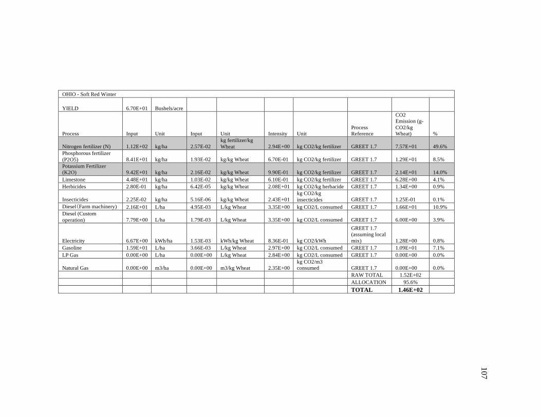
107
OHIO - Soft Red Winter
YIELD 6.70E+01 Bushels/acre
Process Input Unit Input Unit Intensity Unit Process Reference
CO2 Emission (g-CO2/kg Wheat) %
Nitrogen fertilizer (N) 1.12E+02 kg/ha 2.57E-02 kg fertilizer/kg Wheat 2.94E+00 kg CO2/kg fertilizer GREET 1.7 7.57E+01 49.6%
Phosphorous fertilizer (P2O5) 8.41E+01 kg/ha 1.93E-02 kg/kg Wheat 6.70E-01 kg CO2/kg fertilizer GREET 1.7 1.29E+01 8.5% Potassium Fertilizer (K2O) 9.42E+01 kg/ha 2.16E-02 kg/kg Wheat 9.90E-01 kg CO2/kg fertilizer GREET 1.7 2.14E+01 14.0% Limestone 4.48E+01 kg/ha 1.03E-02 kg/kg Wheat 6.10E-01 kg CO2/kg fertilizer GREET 1.7 6.28E+00 4.1% Herbicides 2.80E-01 kg/ha 6.42E-05 kg/kg Wheat 2.08E+01 kg CO2/kg herbacide GREET 1.7 1.34E+00 0.9%
Insecticides 2.25E-02 kg/ha 5.16E-06 kg/kg Wheat 2.43E+01 kg CO2/kg insecticides GREET 1.7 1.25E-01 0.1%
Diesel!Farm machinery) 2.16E+01 L/ha 4.95E-03 L/kg Wheat 3.35E+00 kg CO2/L consumed GREET 1.7 1.66E+01 10.9% Diesel (Custom operation) 7.79E+00 L/ha 1.79E-03 L/kg Wheat 3.35E+00 kg CO2/L consumed GREET 1.7 6.00E+00 3.9%
Electricity 6.67E+00 kWh/ha 1.53E-03 kWh/kg Wheat 8.36E-01 kg CO2/kWh
GREET 1.7 (assuming local mix) 1.28E+00 0.8%
Gasoline 1.59E+01 L/ha 3.66E-03 L/kg Wheat 2.97E+00 kg CO2/L consumed GREET 1.7 1.09E+01 7.1% LP Gas 0.00E+00 L/ha 0.00E+00 L/kg Wheat 2.84E+00 kg CO2/L consumed GREET 1.7 0.00E+00 0.0%
Natural Gas 0.00E+00 m3/ha 0.00E+00 m3/kg Wheat 2.35E+00 kg CO2/m3 consumed GREET 1.7 0.00E+00 0.0%
RAW TOTAL 1.52E+02 ALLOCATION 95.6%
TOTAL 1.46E+02

108
OREGON - Soft White
YIELD 5.40E+01 Bushels/acre
Process Input Unit Input Unit Intensity Unit Process Reference
CO2 Emission (g-CO2/kg Wheat) %
Nitrogen fertilizer (N) 7.90E+01 kg/ha 2.25E-02 kg fertilizer/kg Wheat 2.94E+00 kg CO2/kg fertilizer GREET 1.7 6.62E+01 35.7%
Phosphorous fertilizer (P2O5) 5.10E+01 kg/ha 1.45E-02 kg/kg Wheat 6.70E-01 kg CO2/kg fertilizer GREET 1.7 9.73E+00 5.3% Potassium Fertilizer (K2O) 4.71E+01 kg/ha 1.34E-02 kg/kg Wheat 9.90E-01 kg CO2/kg fertilizer GREET 1.7 1.33E+01 7.2% Limestone 4.48E+01 kg/ha 1.28E-02 kg/kg Wheat 6.10E-01 kg CO2/kg fertilizer GREET 1.7 7.79E+00 4.2% Herbicides 2.80E-01 kg/ha 7.98E-05 kg/kg Wheat 2.08E+01 kg CO2/kg herbacide GREET 1.7 1.66E+00 0.9%
Insecticides 2.01E-02 kg/ha 5.72E-06 kg/kg Wheat 2.43E+01 kg CO2/kg insecticides GREET 1.7 1.39E-01 0.1%
Diesel!Farm machinery) 5.81E+01 L/ha 1.65E-02 L/kg Wheat 3.35E+00 kg CO2/L consumed GREET 1.7 5.55E+01 29.9% Diesel (Custom operation) 7.79E+00 L/ha 2.22E-03 L/kg Wheat 3.35E+00 kg CO2/L consumed GREET 1.7 7.44E+00 4.0%
Electricity 5.07E+01 kWh/ha 1.44E-02 kWh/kg Wheat 2.62E-01 kg CO2/kWh
GREET 1.7 (assuming local mix) 3.78E+00 2.0%
Gasoline 2.34E+01 L/ha 6.67E-03 L/kg Wheat 2.97E+00 kg CO2/L consumed GREET 1.7 1.98E+01 10.7% LP Gas 0.00E+00 L/ha 0.00E+00 L/kg Wheat 2.84E+00 kg CO2/L consumed GREET 1.7 0.00E+00 0.0%
Natural Gas 0.00E+00 m3/ha 0.00E+00 m3/kg Wheat 2.35E+00 kg CO2/m3 consumed GREET 1.7 0.00E+00 0.0%
RAW TOTAL 1.85E+02 ALLOCATION 96.2%
TOTAL 1.78E+02

109
IDAHO - Soft White
YIELD 8.20E+01 Bushels/acre
Process Input Unit Input Unit Intensity Unit Process Reference
CO2 Emission (g-CO2/kg Wheat) %
Nitrogen fertilizer (N) 1.43E+02 kg/ha 2.68E-02 kg fertilizer/kg Wheat 2.94E+00 kg CO2/kg fertilizer GREET 1.7 7.88E+01 49.8%
Phosphorous fertilizer (P2O5) 4.54E+01 kg/ha 8.52E-03 kg/kg Wheat 6.70E-01 kg CO2/kg fertilizer GREET 1.7 5.71E+00 3.6% Potassium Fertilizer (K2O) 3.53E+01 kg/ha 6.62E-03 kg/kg Wheat 9.90E-01 kg CO2/kg fertilizer GREET 1.7 6.56E+00 4.1% Limestone 4.48E+01 kg/ha 8.41E-03 kg/kg Wheat 6.10E-01 kg CO2/kg fertilizer GREET 1.7 5.13E+00 3.2% Herbicides 2.80E-01 kg/ha 5.25E-05 kg/kg Wheat 2.08E+01 kg CO2/kg herbacide GREET 1.7 1.09E+00 0.7%
Insecticides 2.01E-02 kg/ha 3.76E-06 kg/kg Wheat 2.43E+01 kg CO2/kg insecticides GREET 1.7 9.15E-02 0.1%
Diesel!Farm machinery) 4.50E+01 L/ha 8.44E-03 L/kg Wheat 3.35E+00 kg CO2/L consumed GREET 1.7 2.83E+01 17.9% Diesel (Custom operation) 7.79E+00 L/ha 1.46E-03 L/kg Wheat 3.35E+00 kg CO2/L consumed GREET 1.7 4.90E+00 3.1%
Electricity 1.01E+03 kWh/ha 1.89E-01 kWh/kg Wheat 1.05E-01 kg CO2/kWh
GREET 1.7 (assuming local mix) 1.98E+01 12.5%
Gasoline 1.41E+01 L/ha 2.64E-03 L/kg Wheat 2.97E+00 kg CO2/L consumed GREET 1.7 7.84E+00 5.0% LP Gas 0.00E+00 L/ha 0.00E+00 L/kg Wheat 2.84E+00 kg CO2/L consumed GREET 1.7 0.00E+00 0.0%
Natural Gas 0.00E+00 m3/ha 0.00E+00 m3/kg Wheat 2.35E+00 kg CO2/m3 consumed GREET 1.7 0.00E+00 0.0%
RAW TOTAL 1.58E+02 ALLOCATION 96.2%
TOTAL 1.52E+02

110
WASHINGTON - Soft White
YIELD 5.85E+01 Bushels/acre
Process Input Unit Input Unit Intensity Unit Process Reference
CO2 Emission (g-CO2/kg Wheat) %
Nitrogen fertilizer (N) 1.00E+02 kg/ha 2.64E-02 kg fertilizer/kg Wheat 2.94E+00 kg CO2/kg fertilizer GREET 1.7 7.75E+01 46.7%
Phosphorous fertilizer (P2O5) 2.69E+01 kg/ha 7.07E-03 kg/kg Wheat 6.70E-01 kg CO2/kg fertilizer GREET 1.7 4.74E+00 2.9% Potassium Fertilizer (K2O) 3.98E+01 kg/ha 1.05E-02 kg/kg Wheat 9.90E-01 kg CO2/kg fertilizer GREET 1.7 1.04E+01 6.2% Limestone 4.48E+01 kg/ha 1.18E-02 kg/kg Wheat 6.10E-01 kg CO2/kg fertilizer GREET 1.7 7.19E+00 4.3% Herbicides 2.80E-01 kg/ha 7.35E-05 kg/kg Wheat 2.08E+01 kg CO2/kg herbacide GREET 1.7 1.53E+00 0.9%
Insecticides 2.25E-02 kg/ha 5.91E-06 kg/kg Wheat 2.43E+01 kg CO2/kg insecticides GREET 1.7 1.44E-01 0.1%
Diesel!Farm machinery) 5.15E+01 L/ha 1.36E-02 L/kg Wheat 3.35E+00 kg CO2/L consumed GREET 1.7 4.54E+01 27.4% Diesel (Custom operation) 7.79E+00 L/ha 2.05E-03 L/kg Wheat 3.35E+00 kg CO2/L consumed GREET 1.7 6.87E+00 4.1%
Electricity 4.03E+01 kWh/ha 1.06E-02 kWh/kg Wheat 2.62E-01 kg CO2/kWh
GREET 1.7 (assuming local mix) 2.77E+00 1.7%
Gasoline 1.22E+01 L/ha 3.20E-03 L/kg Wheat 2.97E+00 kg CO2/L consumed GREET 1.7 9.52E+00 5.7% LP Gas 0.00E+00 L/ha 0.00E+00 L/kg Wheat 2.84E+00 kg CO2/L consumed GREET 1.7 0.00E+00 0.0%
Natural Gas 0.00E+00 m3/ha 0.00E+00 m3/kg Wheat 2.35E+00 kg CO2/m3 consumed GREET 1.7 0.00E+00 0.0%
RAW TOTAL 1.66E+02 ALLOCATION 96.2%
TOTAL 1.60E+02
Recommended