○
○
○
○
○
○
○
○
○
○
○
○
○
○
○
○
○
○
○
○
○
○
○
○
○
○
○
○
○
○
○
○
○
○
○
○
○
○
○
○
○
○
○
○
○
○
○
○
○
○
○
○
○
○
○
○
○
○
○
○
○
○
○
○
○
○
○
○
○
○
○
○
○
○
○
○
○
○
○
○
○
○
○
○
○
Developing Stand Density Management Regimes Facilitator’s Guide 3 • 1
Lesson 3 Biological Concepts ofTimber Production1.5 hours
Lesson Objectives
▲ To promote a common understanding of biological principles thatunderlie the effects of density management
▲ To provide an overview of wood quality and forest health as theyrelate to density management.
Method: Introduce the Guidelines – Q&A,Lecturette, Video
▲ Introduce biology section
▲ Show biological concepts video
▲ Go over points to emphasize concepts
▲ Present recent information on wood quality as it relates to density
▲ Review the main points of Pacific Forestry Centre TechnologyTransfer Note No. 12, November 1998 regarding forest health anddensity management.
Audio Visual Requirements
▲ Overhead projector
Handout
▲ Technology Transfer Note No. 12, November 1998
Facilitator’s Guide 3 • 2 Information Session
3 • 1
Why Do Density Management?
○
○
○
○
○
○
○
○
○
○
○
○
○
○
○
○
○
○
○
○
○
○
○
○
○
○
○
○
○
○
○
○
○
○
○
○
○
○
○
○
○
○
○
○
○
○
○
○
○
○
○
○
○
○
○
○
○
○
○
○
○
○
○
○
○
○
○
○
○
○
○
○
○
○
○
○
○
○
○
○
○
○
○
○
○
Developing Stand Density Management Regimes Facilitator’s Guide 3 • 3
Benefits of Density Management
▲ Turn to your neighbour exercise – 5 minutes for contemplation,10 minutes to summarize as a group.
What possible management objectives do you believe densitymanagement (particularly pct [pre-commercial thinning])will achieve?
▲ Alleviate timber supply gaps
▲ Improve habitat or riparian function
▲ Set up stands for future entries
▲ Reduce risk of blowdown or snow damage
Any others?
▲ Employ forest workers
Mention only:
Pruning
▲ Provides clear wood
Fertilization
▲ Additional volume if all things go well (i.e., appropriate site, speciesand treatment).
We will concentrate on density manangement.
We now want to translate the objectives from above to identify structuralattributes that are behind the assumptions.
How does density affect individual tree growth and volumeproduction? (from the executive summary)
▲ Stands regenerated or spaced (pct) to relatively high densities(e.g., 1500–10 000 trees/ha) have small differences in volumeand diameter at harvest.
▲ Stands regenerated or spaced (pct) to relatively low densities(e.g., 250–1000 trees/ha) have larger piece sizes at harvest becausemore growing space is available to each tree, lower volumes perhectare because of slow site occupancy following treatment, andlonger biological rotations.
▲ That is, there is a trade-off between tree diameter and stand volumewhich is most clearly reflected in stand and stock tables as opposed tovolume per hectare and average diameter. The diameter benefits ofspacing diminish the longer treatment is delayed beyond crown closure
We will look more closely at the key factors that influence themagnitude of the generalized statements provided.

Facilitator’s Guide 3 • 4 Information Session
○
○
○
○
○
○
○
○
○
○
○
○
○
○
○
○
○
○
○
○
○
○
○
○
○
○
○
○
○
○
○
○
○
○
○
○
○
○
○
○
○
○
○
○
○
○
○
○
○
○
○
○
○
○
○
○
○
○
○
○
○
○
○
○
○
○
○
○
○
○
○
○
○
○
○
○
○
○
○
○
○
○
○
○
○
3 • 2
Volume Over Time – The Basics
Volume
Stand age or time
Stage 1 Stage 2 Stage 3
Mean annualincrement (mai)
Maximum MAI(Culmination)
○
○
○
○
○
○
○
○
○
○
○
○
○
○
○
○
○
○
○
○
○
○
○
○
○
○
○
○
○
○
○
○
○
○
○
○
○
○
○
○
○
○
○
○
○
○
○
○
○
○
○
○
○
○
○
○
○
○
○
○
○
○
○
○
○
○
○
○
○
○
○
○
○
○
○
○
○
○
○
○
○
○
○
○
○
Developing Stand Density Management Regimes Facilitator’s Guide 3 • 5
Growth and Yield – Measures Over Time
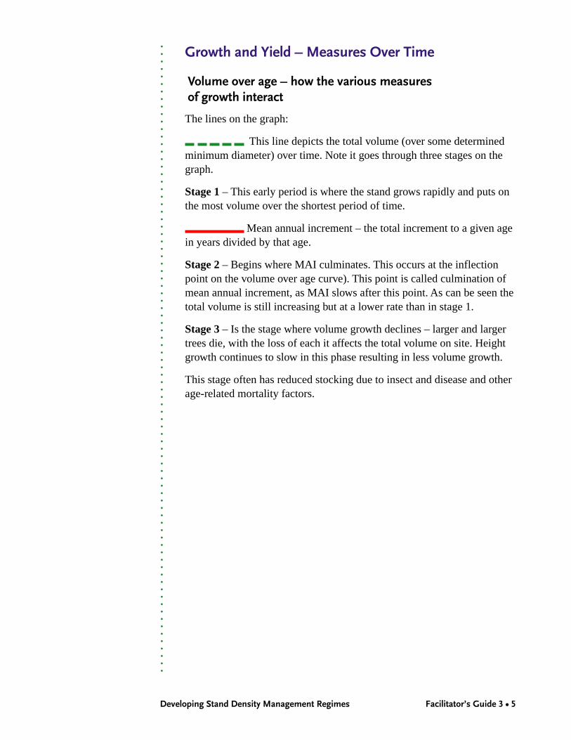
Volume over age – how the various measuresof growth interact
The lines on the graph:
This line depicts the total volume (over some determinedminimum diameter) over time. Note it goes through three stages on thegraph.
Stage 1 – This early period is where the stand grows rapidly and puts onthe most volume over the shortest period of time.
Mean annual increment – the total increment to a given agein years divided by that age.
Stage 2 – Begins where MAI culminates. This occurs at the inflectionpoint on the volume over age curve). This point is called culmination ofmean annual increment, as MAI slows after this point. As can be seen thetotal volume is still increasing but at a lower rate than in stage 1.
Stage 3 – Is the stage where volume growth declines – larger and largertrees die, with the loss of each it affects the total volume on site. Heightgrowth continues to slow in this phase resulting in less volume growth.
This stage often has reduced stocking due to insect and disease and otherage-related mortality factors.

Facilitator’s Guide 3 • 6 Information Session
FIXED
3 • 3
Site productivity is relatively
FIXEDClimate and site
dictate productivity.
Volume Over Time – The Basics
○
○
○
○
○
○
○
○
○
○
○
○
○
○
○
○
○
○
○
○
○
○
○
○
○
○
○
○
○
○
○
○
○
○
○
○
○
○
○
○
○
○
○
○
○
○
○
○
○
○
○
○
○
○
○
○
○
○
○
○
○
○
○
○
○
○
○
○
○
○
○
○
○
○
○
○
○
○
○
○
○
○
○
○
○
Developing Stand Density Management Regimes Facilitator’s Guide 3 • 7
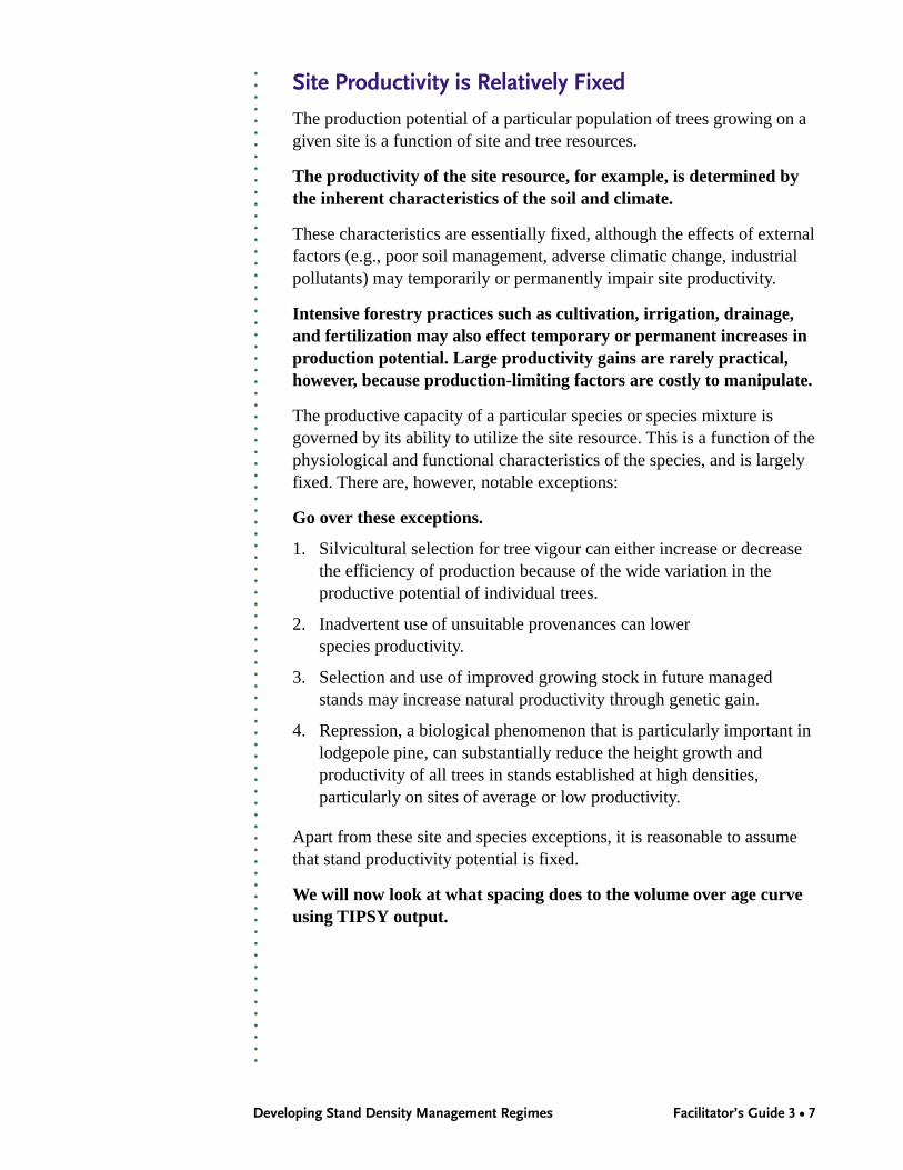
Site Productivity is Relatively Fixed
The production potential of a particular population of trees growing on agiven site is a function of site and tree resources.
The productivity of the site resource, for example, is determined bythe inherent characteristics of the soil and climate.
These characteristics are essentially fixed, although the effects of externalfactors (e.g., poor soil management, adverse climatic change, industrialpollutants) may temporarily or permanently impair site productivity.
Intensive forestry practices such as cultivation, irrigation, drainage,and fertilization may also effect temporary or permanent increases inproduction potential. Large productivity gains are rarely practical,however, because production-limiting factors are costly to manipulate.
The productive capacity of a particular species or species mixture isgoverned by its ability to utilize the site resource. This is a function of thephysiological and functional characteristics of the species, and is largelyfixed. There are, however, notable exceptions:
Go over these exceptions.
1. Silvicultural selection for tree vigour can either increase or decreasethe efficiency of production because of the wide variation in theproductive potential of individual trees.
2. Inadvertent use of unsuitable provenances can lowerspecies productivity.
3. Selection and use of improved growing stock in future managedstands may increase natural productivity through genetic gain.
4. Repression, a biological phenomenon that is particularly important inlodgepole pine, can substantially reduce the height growth andproductivity of all trees in stands established at high densities,particularly on sites of average or low productivity.
Apart from these site and species exceptions, it is reasonable to assumethat stand productivity potential is fixed.
We will now look at what spacing does to the volume over age curveusing TIPSY output.
Facilitator’s Guide 3 • 8 Information Session
3 • 4
Volume Over Time – TIPSY Runs
Using TIPSY to see howdensity affects volume

○
○
○
○
○
○
○
○
○
○
○
○
○
○
○
○
○
○
○
○
○
○
○
○
○
○
○
○
○
○
○
○
○
○
○
○
○
○
○
○
○
○
○
○
○
○
○
○
○
○
○
○
○
○
○
○
○
○
○
○
○
○
○
○
○
○
○
○
○
○
○
○
○
○
○
○
○
○
○
○
○
○
○
○
○
Developing Stand Density Management Regimes Facilitator’s Guide 3 • 9
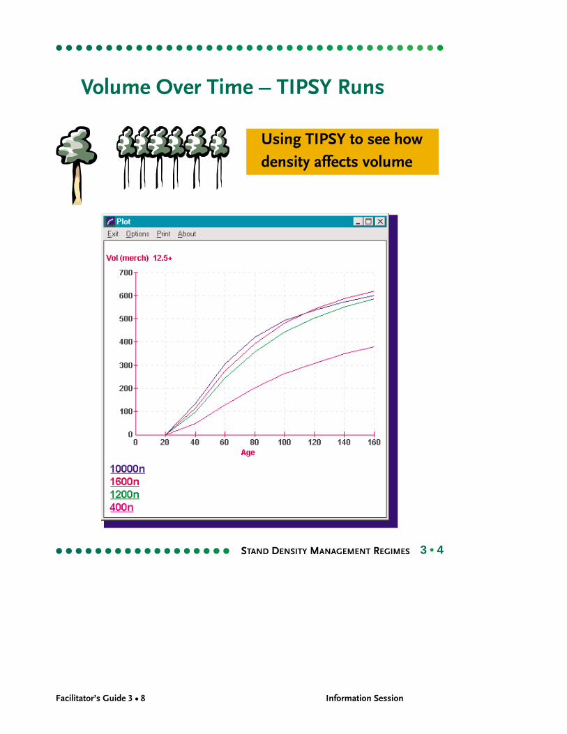
TIPSY OutputTIPSY is the acronym for Table Interpolation Program for Stand Yields –from a database generated by the growth model TASS. TIPSY wasoriginally created in May 1991. TASS is an abbreviation for Tree andStand Simulator. It is a biologically oriented model. It grows stands treeby tree in a three dimensional space in a computer and simulatessilvicultural treatments.
This diagram shows TIPSY over age runs of Pl SI 20 withno OAF adjustments for starting densities of 10 000 sph, 1600 sph,1200 sph and 400 sph (all natural regeneration).
Facilitator’s Guide 3 • 10 Information Session
3 • 5
Stand Production
Stand volume
Stand age
RoughIntermediateClose
Maximum MAI
Utilization:
Gross productionStanding volume
Stand production:
Mortality
○
○
○
○
○
○
○
○
○
○
○
○
○
○
○
○
○
○
○
○
○
○
○
○
○
○
○
○
○
○
○
○
○
○
○
○
○
○
○
○
○
○
○
○
○
○
○
○
○
○
○
○
○
○
○
○
○
○
○
○
○
○
○
○
○
○
○
○
○
○
○
○
○
○
○
○
○
○
○
○
○
○
○
○
○
Developing Stand Density Management Regimes Facilitator’s Guide 3 • 11
Stand production
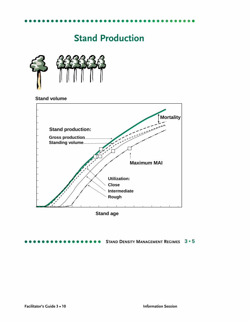
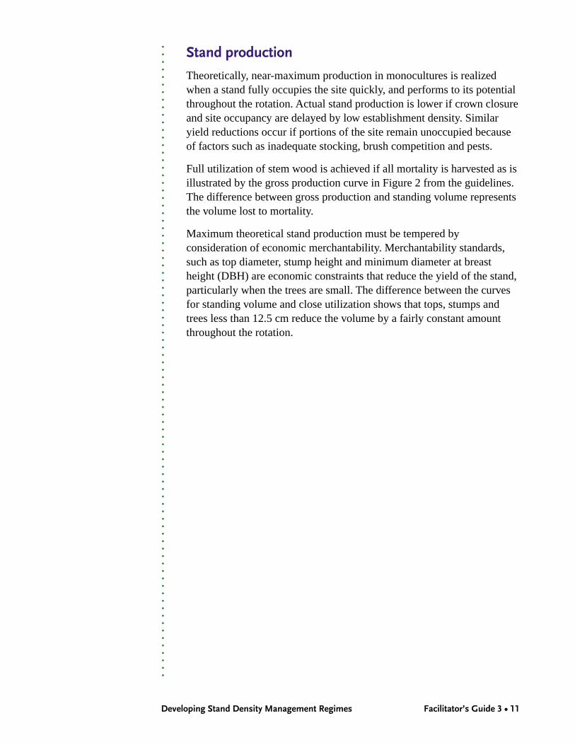
Theoretically, near-maximum production in monocultures is realizedwhen a stand fully occupies the site quickly, and performs to its potentialthroughout the rotation. Actual stand production is lower if crown closureand site occupancy are delayed by low establishment density. Similaryield reductions occur if portions of the site remain unoccupied becauseof factors such as inadequate stocking, brush competition and pests.
Full utilization of stem wood is achieved if all mortality is harvested as isillustrated by the gross production curve in Figure 2 from the guidelines.The difference between gross production and standing volume representsthe volume lost to mortality.
Maximum theoretical stand production must be tempered byconsideration of economic merchantability. Merchantability standards,such as top diameter, stump height and minimum diameter at breastheight (DBH) are economic constraints that reduce the yield of the stand,particularly when the trees are small. The difference between the curvesfor standing volume and close utilization shows that tops, stumps andtrees less than 12.5 cm reduce the volume by a fairly constant amountthroughout the rotation.
Facilitator’s Guide 3 • 12 Information Session
3 • 6
TIPSY Runs
TIPSY derived diameterdistribution fromdifferent densities

○
○
○
○
○
○
○
○
○
○
○
○
○
○
○
○
○
○
○
○
○
○
○
○
○
○
○
○
○
○
○
○
○
○
○
○
○
○
○
○
○
○
○
○
○
○
○
○
○
○
○
○
○
○
○
○
○
○
○
○
○
○
○
○
○
○
○
○
○
○
○
○
○
○
○
○
○
○
○
○
○
○
○
○
○
Developing Stand Density Management Regimes Facilitator’s Guide 3 • 13
TIPSY Output
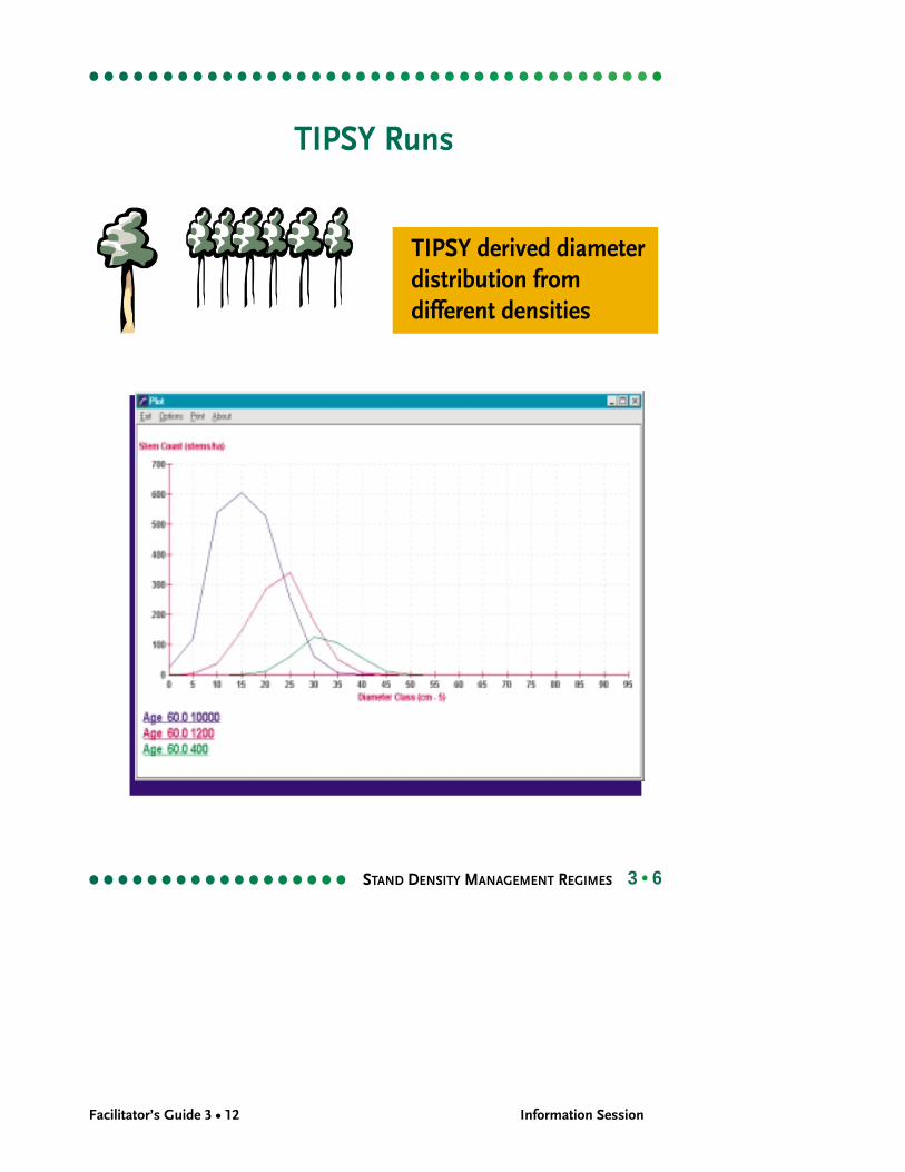
One of the main objectives of pre-commercial thinning (pct) is growinglarger stems faster. The following TIPSY graph shows how TIPSYderived stems are distributed at year 60 for the same Pl SI 20 stand.
The tree lines are for 10 000 naturals/ha, 10 000 naturals pre-commercially thinned to 1200 sph, 10 000 naturals pre-commerciallythinned to 400 sph.
▲ You will note that all have bell shaped distributions.
▲ There are significantly fewer stems in the thinned stands and ingeneral, the stems are larger.
▲ The smallest stems were removed from the thinned stands.
What this means is we will have fewer logs to handle, a more uniformpiece size, with a limited number of larger stems overall. We will stillhave a range of diameters including some smaller stems. For the mostpart we will not have an assemblage of only large trees.
Let us now look at an example showing this response with real data.In BC we do not have many long term spacing trails. We do have theSchenstrom plots at Cowichan Lake (multiple thinnings) established in1929, but due to the multiple entries looking at results is complex.Instead we will look at a simple spacing trial for Hw established in thePacific Northwest in the 1960s.
Facilitator’s Guide 3 • 14 Information Session
3 • 7
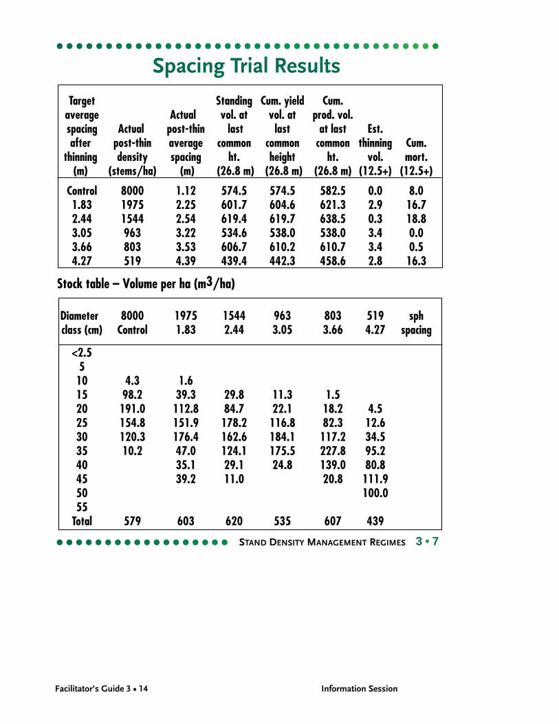
Spacing Trial Results
Target Standing Cum. yield Cum.average Actual vol. at vol. at prod. vol.spacing Actual post-thin last last at last Est.after post-thin average common common common thinning Cum.
thinning density spacing ht. height ht. vol. mort.(m) (stems/ha) (m) (26.8 m) (26.8 m) (26.8 m) (12.5+) (12.5+)
Control 8000 1.12 574.5 574.5 582.5 0.0 8.01.83 1975 2.25 601.7 604.6 621.3 2.9 16.72.44 1544 2.54 619.4 619.7 638.5 0.3 18.83.05 963 3.22 534.6 538.0 538.0 3.4 0.03.66 803 3.53 606.7 610.2 610.7 3.4 0.54.27 519 4.39 439.4 442.3 458.6 2.8 16.3
Stock table – Volume per ha (m3/ha)
Diameter 8000 1975 1544 963 803 519 sphclass (cm) Control 1.83 2.44 3.05 3.66 4.27 spacing
<2.5510 4.3 1.615 98.2 39.3 29.8 11.3 1.520 191.0 112.8 84.7 22.1 18.2 4.525 154.8 151.9 178.2 116.8 82.3 12.630 120.3 176.4 162.6 184.1 117.2 34.535 10.2 47.0 124.1 175.5 227.8 95.240 35.1 29.1 24.8 139.0 80.845 39.2 11.0 20.8 111.950 100.055
Total 579 603 620 535 607 439
○
○
○
○
○
○
○
○
○
○
○
○
○
○
○
○
○
○
○
○
○
○
○
○
○
○
○
○
○
○
○
○
○
○
○
○
○
○
○
○
○
○
○
○
○
○
○
○
○
○
○
○
○
○
○
○
○
○
○
○
○
○
○
○
○
○
○
○
○
○
○
○
○
○
○
○
○
○
○
○
○
○
○
○
○
Developing Stand Density Management Regimes Facilitator’s Guide 3 • 15
Data from a Coastal Experiment
This is data from a Hw pre-commercial thinning trial conducted on theOlympic Peninsula (established in the 1960s). The following tableprovides a summary of treatments and volume at the last commonmeasurement height (28.6 m). The site was monitored from age 13 to 38,the site index is 36 m SI50.
Facilitator’s Guide 3 • 16 Information Session
3 • 8
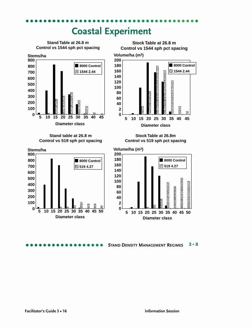
Coastal ExperimentStand Table at 26.8 m
Control vs 1544 sph pct spacing
0100200300400500600700800900Stems/ha
5 10 15 20 25 30 35 40 45
Diameter class
8000 Control
1544 2.44
Stock Table at 26.8 mControl vs 1544 sph pct spacing
02
406080
100120140160180200Volume/ha (m3)
5 10 15 20 25 30 35 40 45
Diameter class
8000 Control
1544 2.44
Stock Table at 26.8mControl vs 519 sph pct spacing
Volume/ha (m3)
8000 Control
519 4.27
5 10 15 20 25 30 35 40 45Diameter class
5002
406080
100120140160180200
Stand table at 26.8 mControl vs 519 sph pct spacing
0100200300400500600700800900Stems/ha
8000 Control
519 4.27
5 10 15 20 25 30 35 40 45Diameter class
50
○
○
○
○
○
○
○
○
○
○
○
○
○
○
○
○
○
○
○
○
○
○
○
○
○
○
○
○
○
○
○
○
○
○
○
○
○
○
○
○
○
○
○
○
○
○
○
○
○
○
○
○
○
○
○
○
○
○
○
○
○
○
○
○
○
○
○
○
○
○
○
○
○
○
○
○
○
○
○
○
○
○
○
○
○
Developing Stand Density Management Regimes Facilitator’s Guide 3 • 17
Data from a Coastal Experiment
Facilitator’s Guide 3 • 18 Information Session
3 • 9
Variation in Growth – Espacement
How Trees Growin the Forest
Stan
d A
geO
ldYo
ung
Ope
n G
row
th
Plastic-differentiation
Tree Spacing NarrowWide
○
○
○
○
○
○
○
○
○
○
○
○
○
○
○
○
○
○
○
○
○
○
○
○
○
○
○
○
○
○
○
○
○
○
○
○
○
○
○
○
○
○
○
○
○
○
○
○
○
○
○
○
○
○
○
○
○
○
○
○
○
○
○
○
○
○
○
○
○
○
○
○
○
○
○
○
○
○
○
○
○
○
○
○
○
Developing Stand Density Management Regimes Facilitator’s Guide 3 • 19
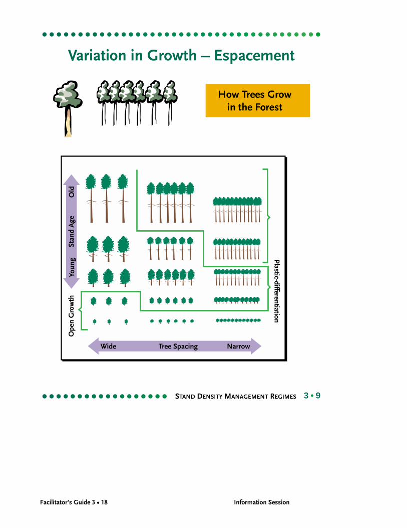
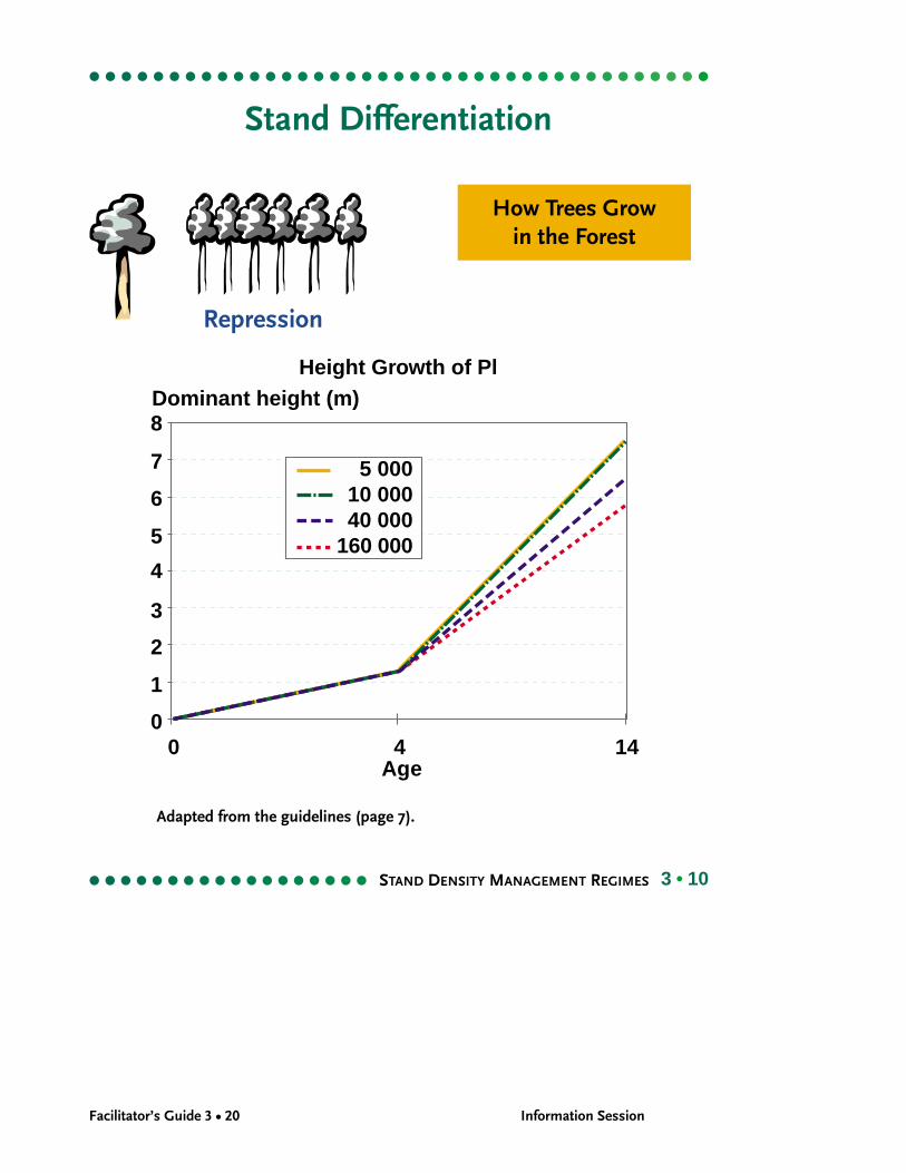
How Forests Grow
The next series of overheads are adaptations of the stand structural stagesas described in Oliver and Larson, 1996. They show how stands grow andwhat various factors will influence growth and hence data collection andtreatment decisions.
▲ What constitutes wide versus narrow. Wide spacing is likely nearminimum stocking values (700 sph is 4.06 m intertree distance usingtriangular spacing, 400 sph is 5.37 m.) Dense spacing likely means10 000 sph plus.
▲ The left axis shows young open grown at the bottom and old above.
What is being influenced by tree spacing?
▲ Tree height – the most dense stand is the shortest and has the leastlive crown.
Is this conventional wisdom? Is this how it works in the real world?
▲ For Pl above a certain density it does (from 10 000 to 30 000 totalstems per ha are densities where height repression can begin for Pl).This phenomenon is called height repression and will bediscussed later.
What is it about this stand structure that seems somewhat peculiar?
▲ No differentiation – all trees are the same size. Normally there will besome form of differentiation, unless there is no genetic or micrositevariation (e.g., cones in a farm field).
KEY – in BC repression has been found in Pl. To avoid reducedheights and volumes, treatment is required to reduce density .
Facilitator’s Guide 3 • 20 Information Session
3 • 10
Stand Differentiation
How Trees Growin the Forest
Height Growth of Pl
0
1
2
3
4
5
6
7
8
0 4 14Age
Dominant height (m)
5 00010 00040 000
160 000
Adapted from the guidelines (page 7).
Repression
○
○
○
○
○
○
○
○
○
○
○
○
○
○
○
○
○
○
○
○
○
○
○
○
○
○
○
○
○
○
○
○
○
○
○
○
○
○
○
○
○
○
○
○
○
○
○
○
○
○
○
○
○
○
○
○
○
○
○
○
○
○
○
○
○
○
○
○
○
○
○
○
○
○
○
○
○
○
○
○
○
○
○
○
○
Developing Stand Density Management Regimes Facilitator’s Guide 3 • 21
Repression
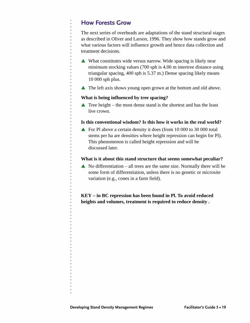
Repression is a biological phenomenon whereby tree growth and standdevelopment fail to exploit the potential productivity of the site. Theimpact is widespread (Goudie 1996) in stands of lodgepole pine but notin other species.
Biology
Repression curtails height and volume increment of lodgepole pineshortly after the growing space is fully utilized in stands established atextreme densities. The process usually begins before trees reach a heightof 2.0 metres, although stands with 1 000 000 trees/ha may be affectedwhen only 0.2 metres tall.
Espacement trials (Carlson and Johnstone 1983) show that the heightgrowth of plantations with 13 500 or more planted trees are affected(Figure 1), and future measurements may indicate minor repression instands planted with 10 000 trees. The pattern of growth and developmentof repressed stands resembles that of stands growing on sites of muchlower productivity; consequently, merchantable yields will be achievedconsiderably later than had repression been avoided. Repression doesnot, however, cause stands to “stagnate” or cease development, as wasonce believed.
Impact – Mainly on fire origin stands
Growth losses are particularly dramatic in repressed fire-originstands of lodgepole established with more than 50 000 trees perhectare (Mitchell and Goudie 1980), particularly on sites of relativelylow productivity. At extreme densities (500 000 + trees/ha), standproduction may be reduced by as much as 60 per cent.
Repression is not likely to be a serious problem in stands that regenerateafter logging because establishment densities are much lower, trees seed-in over 5 to 10 years (instead of 2 to 3 years), and clumped (less uniform)tree distributions are more common. The lower densities and greatertree-size diversity of post-logging stands minimizes the risk ofrepression losses.
Repression is also unlikely in plantations, unless supplemented byconcurrent, natural, in-fill regeneration. The impact of dense, butdelayed, natural regeneration on planted lodgepole pine stands is notpresently known.

Facilitator’s Guide 3 • 22 Information Session
○
○
○
○
○
○
○
○
○
○
○
○
○
○
○
○
○
○
○
○
○
○
○
○
○
○
○
○
○
○
○
○
○
○
○
○
○
○
○
○
○
○
○
○
○
○
○
○
○
○
○
○
○
○
○
○
○
○
○
○
○
○
○
○
○
○
○
○
○
○
○
○
○
○
○
○
○
○
○
○
○
○
○
○
○
Developing Stand Density Management Regimes Facilitator’s Guide 3 • 23
Response to Treatment
Stand density interventions are an effective means of preventingrepression in lodgepole pine if treatment occurs before the onset ofrepression. Stands which are thinned after the onset of repression do notshow a consistent height growth response to treatment (J.S. Thrower andAssoc. 1993). However, there is evidence of an independent response indiameter growth.
Until more is known about treatment response it isreasonable to assume that the early height growth ofrepressed stands is indicative of future productivity.
Facilitator’s Guide 3 • 24 Information Session
Growth Variation – Espacement
How Trees Growin the Forest
Stan
d A
geO
ldYo
ung
Tree Spacing NarrowArea I
3 • 11

○
○
○
○
○
○
○
○
○
○
○
○
○
○
○
○
○
○
○
○
○
○
○
○
○
○
○
○
○
○
○
○
○
○
○
○
○
○
○
○
○
○
○
○
○
○
○
○
○
○
○
○
○
○
○
○
○
○
○
○
○
○
○
○
○
○
○
○
○
○
○
○
○
○
○
○
○
○
○
○
○
○
○
○
○
Developing Stand Density Management Regimes Facilitator’s Guide 3 • 25
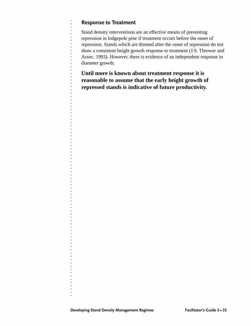
How Stands Grow – The Effect of Espacement
Note this is not the total story.
This overhead depicts the variation in growth due to original spacing.What does the diagram show us?
▲ What the spacing trials show is that trees with more room to growwill have larger crowns and larger diameter growth potential. Densestands will have some stems in understorey positions that will besuppressed by their neighbours.
▲ Area 1 is relatively dense from the start. Crowns lift early resulting inthin stems with reduced growth potential – the clumps found in thisstand show better growth on the edges. Therefore, any treatmentresponse needs to take into account the size of the clumps, the densityin the centre and whether the vigour of the trees is sufficient forresponse if density is reduced. If we wait too long (crowns are nowsmall) diameter increases will be slowed, reducing its effect.
▲ Note (rule of thumb – from OSU Extension Services, 1997, EC 1189)– If the clump is over three crown widths wide, the clump should bemanaged the same as the rest of the stand. If not, leave along theedges slightly closer than the prescribed spacing (they are alreadysomewhat open due to their position on the edge of clump). Don’ tleave overdense areas to compensate for holes in the stand.
▲ The key element of this diagram is that crowns respond differentlydepending upon density. Thus, removing trees from the middle ofclumps and leaving the edges intact will provide more trees access tomore light. This will result in larger crowns, allowing the trees togrow larger.
Facilitator’s Guide 3 • 26 Information Session
Growth Variation – By Genesand Microsite Variation
How Trees Growin the Forest
Stan
d A
geO
ldYo
ung
3 • 12

○
○
○
○
○
○
○
○
○
○
○
○
○
○
○
○
○
○
○
○
○
○
○
○
○
○
○
○
○
○
○
○
○
○
○
○
○
○
○
○
○
○
○
○
○
○
○
○
○
○
○
○
○
○
○
○
○
○
○
○
○
○
○
○
○
○
○
○
○
○
○
○
○
○
○
○
○
○
○
○
○
○
○
○
○
Developing Stand Density Management Regimes Facilitator’s Guide 3 • 27
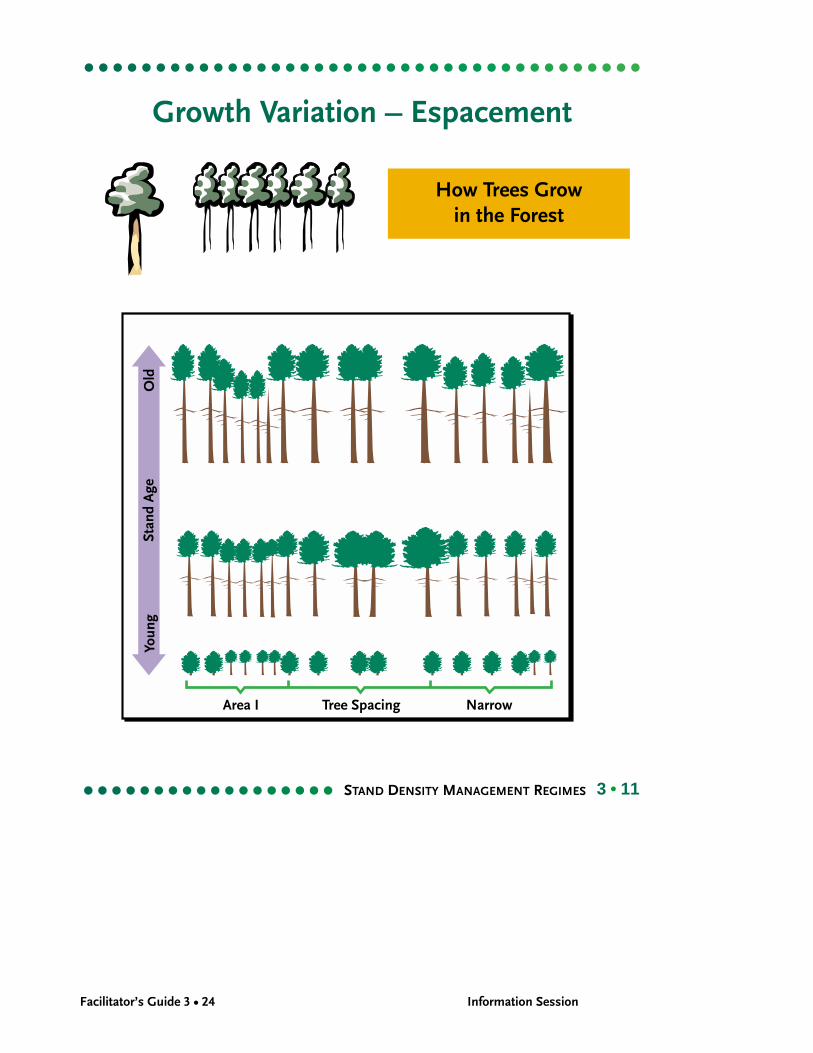
How Stands Grow – Due to Genetic Makeup andMicrosite Variation
Remember: This too is not the total story – what is left? (Differentialestablishment times, different species in the mix.)
This overhead depicts the variation in growth due to microsite andgenetic variation. What does the diagram show us?
▲ Sometimes even where trees are well spaced they will not achieve thesize of others due to genetics and microsite differences.
▲ It is likely good to think in terms of the tree living within aprobability matrix. As the Duke brothers found out in Trading Placesneither nurture nor nature acts alone.
▲ The simplified matrix looks something like this.
Good Microsite Good MicrositeGood Genes Lousy Genes
Big Trees Medium Trees
Poor Microsite Poor MicrositeGood Genes Lousy Genes
Medium Trees Small Trees
Because of this we are likely to get a range of sizes on each site.However as the bottom boxes attest the best we will be able to get onpoor sites are smaller trees within the same time frame as on better sites.
Facilitator’s Guide 3 • 28 Information Session
Timing of EstablishmentStand Differentiation
How Trees Growin the Forest
Stan
d A
geO
ldYo
ung
3 • 13
○
○
○
○
○
○
○
○
○
○
○
○
○
○
○
○
○
○
○
○
○
○
○
○
○
○
○
○
○
○
○
○
○
○
○
○
○
○
○
○
○
○
○
○
○
○
○
○
○
○
○
○
○
○
○
○
○
○
○
○
○
○
○
○
○
○
○
○
○
○
○
○
○
○
○
○
○
○
○
○
○
○
○
○
○
Developing Stand Density Management Regimes Facilitator’s Guide 3 • 29
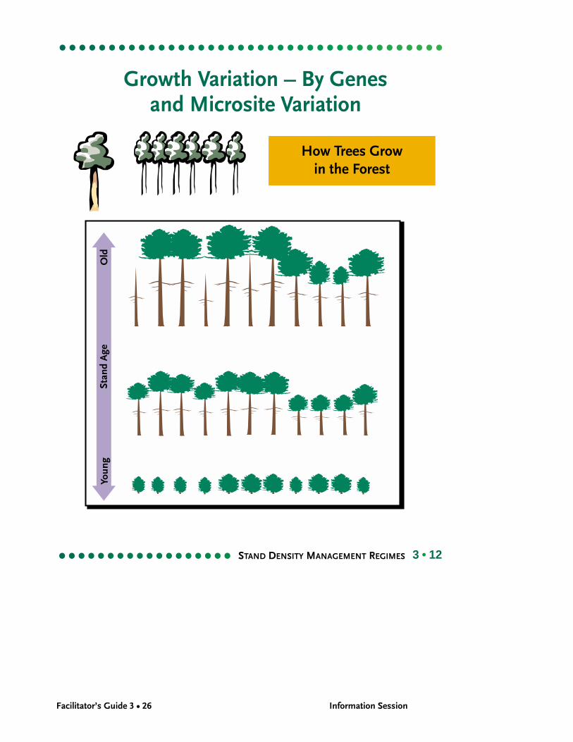
How Stands Grow – Timing of Establishment
This too is not the total story – what is left? (Different speciesin the mix.)
This overhead depicts the variation in growth due to differences in thetime of establishment. What does the diagram show us?
▲ Depending upon stand density and aspect, the late starters will likelynever be in the top portion of the crown (unless they are climaxspecies and outlive the early successional overstorey). Late starterscan be on good sites and have good genes but, if they are slow togrow in the early years, they will not have access to the sun that theirneighbours do, resulting in smaller crowns and less growth.
Stand differentiation
Mortality in stands is natural and will happen with time. One of theobjectives of incremental silvicultural activities is to capture some of thegrowing space that would have gone to mortality and channel it onto apotential crop tree.
Stand differentiation is the result of stand density, genetics, growingenvironment, and time of establishment and is further tangled by multiplespecies. The resultant stand will likely have some dominant trees, mostlycodominants and some intermediate and suppressed trees. The intent ofmost juvenile spacing treatments is to maintain or enhance the diametergrowth of the trees left on site.
We will look now at the role of species in stand differentiation.
Facilitator’s Guide 3 • 30 Information Session
Stand Differentiation – Multiple Species
How Trees Growin the Forest
Multiple Species
0
25
1870 1890 1920 1950 1985
Date (years)
Tree Heightmetresfeet
20
50
75
Larch
Grand fir
Douglas-fir
Gra
nd fi
rD
ougl
as-fi
rLa
rch
Dou
glas
-fir
Larc
hG
rand
fir
10
Oliver and Larson (1996, p. 247)
3 • 14
○
○
○
○
○
○
○
○
○
○
○
○
○
○
○
○
○
○
○
○
○
○
○
○
○
○
○
○
○
○
○
○
○
○
○
○
○
○
○
○
○
○
○
○
○
○
○
○
○
○
○
○
○
○
○
○
○
○
○
○
○
○
○
○
○
○
○
○
○
○
○
○
○
○
○
○
○
○
○
○
○
○
○
○
○
Developing Stand Density Management Regimes Facilitator’s Guide 3 • 31
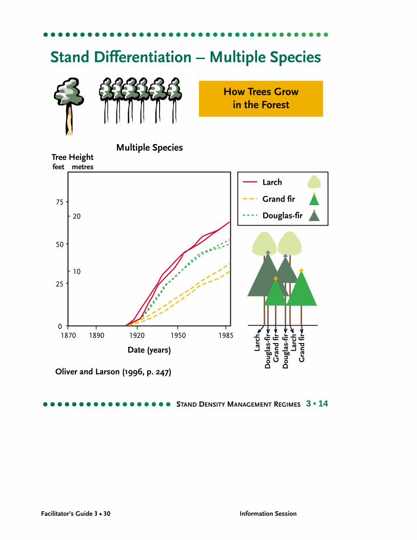
How Stands Grow – Multiple Species
This overhead depicts the variation in growth due to species differences.In some cases species are adapted to grow in an understorey position(e.g., grand fir), or grow with other species (e.g., Fdi and Larch). In othercases, if one species gets a head start on the other species they will likelysuccumb to mortality first resulting in lower numbers of the slowergrowing species after crown closure. In other cases, the initialstratification may change over time if the component species havedifferent patterns of height-growth. For example, the height growth ofpaper birch slows dramatically after about age 40. Other species in thestand may subsequently overtake and surpass the birch in height. Thestratification can also be altered by insects and diseases that pre-ferentially damage and weaken one species or stratum in the mixture.
In stands of mixed species, the variation in tree size is even morepronounced because of the wider range of inherent rates of juvenileheight growth. Stand mixtures of species tend to differentiate intodistinct layers or strata when differences in height growth are large. Thisinitial stratification can persist if the slower-growing species are shadetolerant, or if sufficient sunlight can pass through the foliage of trees inthe upper stratum.
Diameter distributions in mixed-species stands generally reflect theheight stratification. The species in the upper and lower canopy occupythe larger and smaller diameter classes, respectively. If the slower-growing species are shade tolerant, diameter distributions are oftenskewed toward smaller sizes. Broadleaf species sometimes exhibit adifferent height-diameter ratio than conifers and consequentlyappear lower down in the diameter distribution than they are in theheight distribution.
Canopy stratification patterns can be altered if the species with slowerjuvenile height growth have an advantage in early stand development.They may regenerate in advance of the faster-growing species, ordensity control measures may free them from competition during thejuvenile phase of slow growth, thereby ensuring they do not lag farbehind the faster-growing species at the time of stand canopy closure.Silvicultural treatments undertaken at or shortly after establishment cancreate single-layered stands of species that would otherwise naturallyform stratified canopies.

Facilitator’s Guide 3 • 32 Information Session
3 • 15
Stand Differentiation – Multiple Species
How Trees Growin the Forest
Multiple Species
1. Species monoculture
2. Species mixture – substitution
Legend
Species A
Species B
3. Species mixture – addition
○
○
○
○
○
○
○
○
○
○
○
○
○
○
○
○
○
○
○
○
○
○
○
○
○
○
○
○
○
○
○
○
○
○
○
○
○
○
○
○
○
○
○
○
○
○
○
○
○
○
○
○
○
○
○
○
○
○
○
○
○
○
○
○
○
○
○
○
○
○
○
○
○
○
○
○
○
○
○
○
○
○
○
○
○
Developing Stand Density Management Regimes Facilitator’s Guide 3 • 33
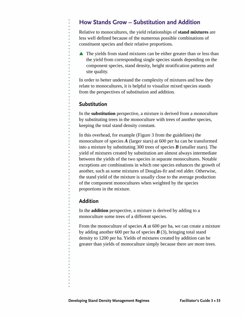
How Stands Grow – Substitution and Addition
Relative to monocultures, the yield relationships of stand mixtures areless well defined because of the numerous possible combinations ofconstituent species and their relative proportions.
▲ The yields from stand mixtures can be either greater than or less thanthe yield from corresponding single species stands depending on thecomponent species, stand density, height stratification patterns andsite quality.
In order to better understand the complexity of mixtures and how theyrelate to monocultures, it is helpful to visualize mixed species standsfrom the perspectives of substitution and addition.
Substitution
In the substitution perspective, a mixture is derived from a monocultureby substituting trees in the monoculture with trees of another species,keeping the total stand density constant.
In this overhead, for example (Figure 3 from the guidelines) themonoculture of species A (larger stars) at 600 per ha can be transformedinto a mixture by substituting 300 trees of species B (smaller stars). Theyield of mixtures created by substitution are almost always intermediatebetween the yields of the two species in separate monocultures. Notableexceptions are combinations in which one species enhances the growth ofanother, such as some mixtures of Douglas-fir and red alder. Otherwise,the stand yield of the mixture is usually close to the average productionof the component monocultures when weighted by the speciesproportions in the mixture.
Addition
In the addition perspective, a mixture is derived by adding to amonoculture some trees of a different species.
From the monoculture of species A at 600 per ha, we can create a mixtureby adding another 600 per ha of species B (3), bringing total standdensity to 1200 per ha. Yields of mixtures created by addition can begreater than yields of monoculture simply because there are more trees.
Facilitator’s Guide 3 • 34 Information Session
3 • 16
Density Management Practices
Espacement
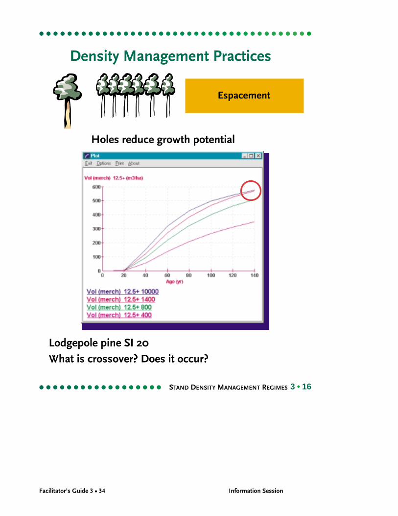
Holes reduce growth potential
Lodgepole pine SI 20What is crossover? Does it occur?

○
○
○
○
○
○
○
○
○
○
○
○
○
○
○
○
○
○
○
○
○
○
○
○
○
○
○
○
○
○
○
○
○
○
○
○
○
○
○
○
○
○
○
○
○
○
○
○
○
○
○
○
○
○
○
○
○
○
○
○
○
○
○
○
○
○
○
○
○
○
○
○
○
○
○
○
○
○
○
○
○
○
○
○
○
Developing Stand Density Management Regimes Facilitator’s Guide 3 • 35
Espacement
Plantation espacement in B.C. since 1940 ranged from:
▲ about 2 metres (2500 trees/ha) to 4 metres (625/ha).
▲ Espacement in natural stands covers a much wider range, for example1–1 000 000 trees/ha., and is much less regular.
▲ Full site occupancy is achieved quickly if the establishment density ismoderately high and the spatial distribution of trees is uniform.Uniformity increases in importance as establishment densitydecreases as more holes will be created.
Volume production in the overhead indicates less volume withdecreasing establishment density. Any clumping of the same number ofstems will reduce the stand yield even further.
It should be noted that it is the unoccupied growing space or “ holes” inthe stand canopy that reduce timber yield – not the clumpiness itself.Low density stands produce less volume initially because there are toofew trees to exploit the available growing space. The rate of stand growthimproves after crown closure.
Cross-over
Theoretically, the growth rate of a low density stand could eventuallysurpass that of a dense stand, as predicted by yield projection models.This phenomenon, called cross-over, has not been observed in researchplots in British Columbia, which are still too young to confirm or rejectthe theory. Ministry data and models predict that cross-over is notlikely to occur until well beyond acceptable rotation ages based onthe culmination of mean annual increment.
Facilitator’s Guide 3 • 36 Information Session
3 • 17
Density Management Practices
Volume Over Timein Spaced Stands
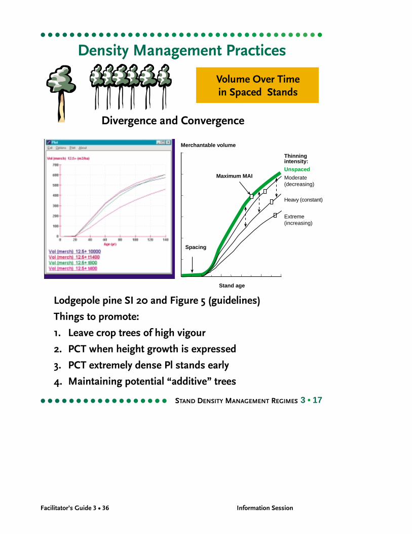
Divergence and Convergence
Lodgepole pine SI 20 and Figure 5 (guidelines)
Things to promote:
1. Leave crop trees of high vigour
2. PCT when height growth is expressed
3. PCT extremely dense Pl stands early
4. Maintaining potential “additive” trees
Merchantable volume
Stand age
Spacing
Maximum MAI
Thinningintensity:Unspaced
Moderate(decreasing)
Heavy (constant)
Extreme(increasing)
○
○
○
○
○
○
○
○
○
○
○
○
○
○
○
○
○
○
○
○
○
○
○
○
○
○
○
○
○
○
○
○
○
○
○
○
○
○
○
○
○
○
○
○
○
○
○
○
○
○
○
○
○
○
○
○
○
○
○
○
○
○
○
○
○
○
○
○
○
○
○
○
○
○
○
○
○
○
○
○
○
○
○
○
○
Developing Stand Density Management Regimes Facilitator’s Guide 3 • 37
Volume Over Time – What Happens to Pre-commerciallyThinned StandsPre-commercial thinning immediately reduces the number of trees, theoccupancy of growing space and the standing volume per hectare.
▲ The magnitude of the reduction is related to the intensity of treatment.
▲ The subsequent development of the stand is more complex.
Crown cover normally increases at a diminishing rate until completecanopy closure occurs, and then levels off.
▲ The number of trees in the spaced stand remains fairly constant untilthe onset of crown closure, competition and mortality.
▲ Volume increment is reduced until the vacant growing space createdby pct is fully utilized by the residual stand.
▲ The corresponding volume curves of the spaced and untreated standswill initially diverge and later parallel one another.
▲ Convergence of the curves usually starts shortly after mortality beginsin the pct stand. The duration of each phase depends on the intensityof pre-commercial thinning and the level of utilization.
If only overtopped trees are removed and 100% crown cover is maintained,convergence will begin immediately without any divergence. On the otherhand, a very heavy spacing will initiate a lengthy phase of divergence thatcould extend until the stand is harvested. Since one phase tends to dominate,volume curves can be described in terms of decreasing, constant orincreasing departure as illustrated in the graph on the right.
The graph on the right (Figure 5 from the guidelines) shows a generalizedsituation. The degree of divergence or convergence will depend upon thesituation. The TIPSY example shows extreme spacing (to 400 sph) results inincreasing departure (divergence), while pct from 10 000 to 1400 actuallyresults in greater volume production than the unspaced stand at 10 000 sph.
Key – at low densities you will lose volume, but not necessarily if youchoose the residual density with this in mind.
Things to avoid
If you are trying to maintain stand volume at the same time as increasing individualtree diameter, avoid:
1. choosing crop trees of low vigour due to uniformity of spacing taking precedence
2. height growth potential is not obvious
3. pre-commercial thinning of extremely dense Pl stands is delayed past the onsetof height repression
4. thinning out shade tolerant species that could add volume by growingin the understorey.

Facilitator’s Guide 3 • 38 Information Session
3 • 18
Commercial Thinning
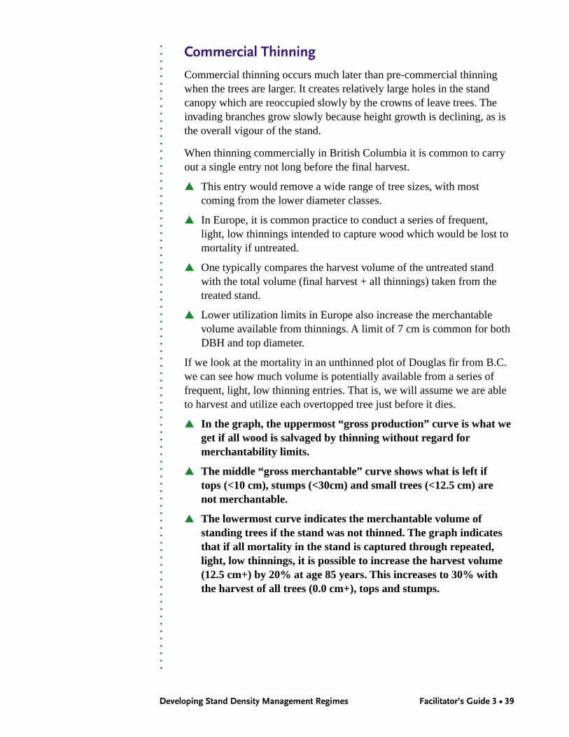
How much volume isavailable from mortality?
Utilization
Potential volume gains
▲ 12.5 cm utilization – 160 m3 (20%)
▲ If all mortality were captured – 350 m3 (30%)
Is this reasonable/realistic?
0
200
400
600
800
1000
1200
1400
1600
50 85Stand age (years)
Volume (m3)
0+0Gross MerchStanding Merch
○
○
○
○
○
○
○
○
○
○
○
○
○
○
○
○
○
○
○
○
○
○
○
○
○
○
○
○
○
○
○
○
○
○
○
○
○
○
○
○
○
○
○
○
○
○
○
○
○
○
○
○
○
○
○
○
○
○
○
○
○
○
○
○
○
○
○
○
○
○
○
○
○
○
○
○
○
○
○
○
○
○
○
○
○
Developing Stand Density Management Regimes Facilitator’s Guide 3 • 39
Commercial Thinning
Commercial thinning occurs much later than pre-commercial thinningwhen the trees are larger. It creates relatively large holes in the standcanopy which are reoccupied slowly by the crowns of leave trees. Theinvading branches grow slowly because height growth is declining, as isthe overall vigour of the stand.
When thinning commercially in British Columbia it is common to carryout a single entry not long before the final harvest.
▲ This entry would remove a wide range of tree sizes, with mostcoming from the lower diameter classes.
▲ In Europe, it is common practice to conduct a series of frequent,light, low thinnings intended to capture wood which would be lost tomortality if untreated.
▲ One typically compares the harvest volume of the untreated standwith the total volume (final harvest + all thinnings) taken from thetreated stand.
▲ Lower utilization limits in Europe also increase the merchantablevolume available from thinnings. A limit of 7 cm is common for bothDBH and top diameter.
If we look at the mortality in an unthinned plot of Douglas fir from B.C.we can see how much volume is potentially available from a series offrequent, light, low thinning entries. That is, we will assume we are ableto harvest and utilize each overtopped tree just before it dies.
▲ In the graph, the uppermost “ gross production” curve is what weget if all wood is salvaged by thinning without regard formerchantability limits.
▲ The middle “ gross merchantable” curve shows what is left iftops (<10 cm), stumps (<30cm) and small trees (<12.5 cm) arenot merchantable.
▲ The lowermost curve indicates the merchantable volume ofstanding trees if the stand was not thinned. The graph indicatesthat if all mortality in the stand is captured through repeated,light, low thinnings, it is possible to increase the harvest volume(12.5 cm+) by 20% at age 85 years. This increases to 30% withthe harvest of all trees (0.0 cm+), tops and stumps.

Facilitator’s Guide 3 • 40 Information Session

○
○
○
○
○
○
○
○
○
○
○
○
○
○
○
○
○
○
○
○
○
○
○
○
○
○
○
○
○
○
○
○
○
○
○
○
○
○
○
○
○
○
○
○
○
○
○
○
○
○
○
○
○
○
○
○
○
○
○
○
○
○
○
○
○
○
○
○
○
○
○
○
○
○
○
○
○
○
○
○
○
○
○
○
○
Developing Stand Density Management Regimes Facilitator’s Guide 3 • 41
The lowermost curve in the graph displays the standing merchantablevolume if the stand was not thinned (pages 16 and 17 in the guidelines).
▲ A series of light entries increases the total harvest because the spacevacated by small-crowned trees is small, and frequent entriesmaximizes the opportunity to salvage trees before they die.
▲ A single heavy entry, timed well before the final harvest, will likelydecrease the total yield because tree removals create large openings,resulting in less than full site occupancy by the residual stand.Furthermore, only one opportunity to harvest impending mortalitywill result in lost volume between thinning and final harvest.

Facilitator’s Guide 3 • 42 Information Session
Thinning
Thinning
3 • 19
Commerical Thinning
What doesresearch tell us?
Standing volume only
1000
500
00 10 20 30 40 50 60 70 80
Standing + thinning volume
1000
500
0
Stand age (years)
Thinning
Thinning
Merchantable volume (m3/ha)
90 100
Merchantable volume (m3/ha)
0 10 20 30 40 50 60 70 80 90 100
Thinning intensity:T3 (Light)T1 (Very light)T0 (Unthinned)T4 (Moderate)
T0 (Unthinned)T1 (Very light)T3 (Light)
T4 (Moderate)
Thinning intensity:
○
○
○
○
○
○
○
○
○
○
○
○
○
○
○
○
○
○
○
○
○
○
○
○
○
○
○
○
○
○
○
○
○
○
○
○
○
○
○
○
○
○
○
○
○
○
○
○
○
○
○
○
○
○
○
○
○
○
○
○
○
○
○
○
○
○
○
○
○
○
○
○
○
○
○
○
○
○
○
○
○
○
○
○
○
Developing Stand Density Management Regimes Facilitator’s Guide 3 • 43
Commercial Thinning
▲ The graph is from research on Coastal Douglas-fir (Omule 1988).Three levels of thinning intensity are shown along with the control.
▲ Volume removed – T1–14%, T3–29%, T4–41%.
▲ The top graph shows how the standing volume of the untreated andthinned plots developed over time. What this shows is the standingvolume will go down with the commercial thinning entry. With thelight thinning levels the volumes begin to converge and if very lightwill result in similar standing volume.
▲ Standing plus thinning volume result in slightly elevated amounts forT1 and T3, (5 and 7%) however they were not statistically significant.
Lower graph
▲ The point being made here is that CT may not effect final yields withlight thinnings. With heavy thinnings the holes in the stand will resultin volume reductions (T4–6%).
In the guidelines a hypothetical example is provided to emphasize howheavy thinnings will result in considerably less total volume.
Facilitator’s Guide 3 • 44 Information Session
3 • 20
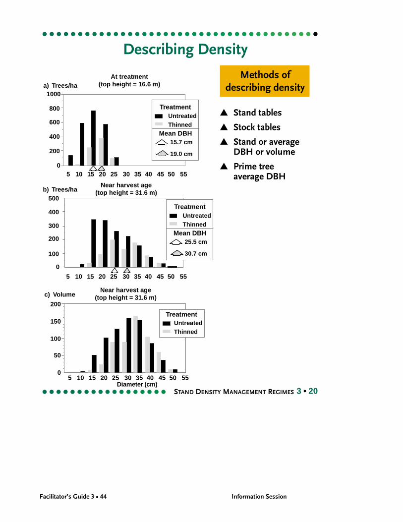
Describing Density
▲ Stand tables
▲ Stock tables
▲ Stand or averageDBH or volume
▲ Prime treeaverage DBH
Near harvest age(top height = 31.6 m)
200
150
100
50
0
c) Volume
Diameter (cm)
Near harvest age(top height = 31.6 m)
500
400
300
200
100
0
b) Trees/ha
At treatment(top height = 16.6 m)a) Trees/ha
1000
800
600
400
200
0
5 10 15 20 25 30 35 40 45 50 55
5 10 15 20 25 30 35 40 45 50 55
5 10 15 20 25 30 35 40 45 50 55
UntreatedThinned
Treatment
UntreatedThinned
Treatment
Mean DBH15.7 cm
19.0 cm
UntreatedThinned
Treatment
Mean DBH25.5 cm
30.7 cm
Methods ofdescribing density
○
○
○
○
○
○
○
○
○
○
○
○
○
○
○
○
○
○
○
○
○
○
○
○
○
○
○
○
○
○
○
○
○
○
○
○
○
○
○
○
○
○
○
○
○
○
○
○
○
○
○
○
○
○
○
○
○
○
○
○
○
○
○
○
○
○
○
○
○
○
○
○
○
○
○
○
○
○
○
○
○
○
○
○
○
Developing Stand Density Management Regimes Facilitator’s Guide 3 • 45
Describing Density
Stand Tables
Stand tables indicate the number of trees, by diameter class, at aparticular stage of stand development.
▲ Good for visualizing what the stand is made up of and where themajority of stems fit.
Stock Tables
A stock table displays volume, by diameter class, and enhances standtable data by identifying the diameters classes which contain the bulk ofthe volume. It is important to focus on the upper and middle diameterclasses of each plot since they contain the trees of greatest volume.
▲ Good for visualizing where the bulk of the volume is concentrated
▲ Graph (c) illustrates a stock table comparison of the thinned andunthinned plots at 31.6 m of top height.
▲ Note that the “extra wood” in the unthinned stand is concentrated inthe smallest diameter classes.
Stand Average DBH or Volume
The average diameter or volume of all trees in the stand provides a usefulbut narrow view of a stand, compared with a stand and stock tablesummary of stand structure.
▲ For example, in graph (a) thinning from below instantly raises theaverage diameter of the plot (15.7 to 19.0 cm) in what is known as the“chainsaw effect”. This is caused by the removal of small trees duringthinning, which inflates the arithmetic average diameter of theremaining trees.

Facilitator’s Guide 3 • 46 Information Session

○
○
○
○
○
○
○
○
○
○
○
○
○
○
○
○
○
○
○
○
○
○
○
○
○
○
○
○
○
○
○
○
○
○
○
○
○
○
○
○
○
○
○
○
○
○
○
○
○
○
○
○
○
○
○
○
○
○
○
○
○
○
○
○
○
○
○
○
○
○
○
○
○
○
○
○
○
○
○
○
○
○
○
○
○
Developing Stand Density Management Regimes Facilitator’s Guide 3 • 47
Prime Tree Average DBH
If there is a wide range of establishment densities, it is useful to comparethe development of prime trees (largest 250 trees/ha) because these treeswill likely survive to harvest in all stands. Furthermore, prime trees areindependent of the chainsaw effect in stands thinned from below. Forexample, the average diameter of the prime trees in the thinned andunthinned stands is 38.3 and 37.5 respectively.
▲ The prime trees in the thinned stand outgrew those in the unthinnedstand, but the difference is small because prime trees do not sufferfrom the same intensity of competition as smaller trees in the stand.Prime tree diameter is largely insensitive to stand density, unless theinter-tree distance is quite large. For example, the stand depicted inthe overhead was thinned late (16.6 m) to a residual density of750 trees which will only stimulate the growth of prime trees for ashort period.
In summary, while average diameter of prime trees and standaverage diameter are informative statistics, they must be usedcautiously when assessing stand response to density management.Both statistics have shortcomings in portraying stand structure, andneither should be used in isolation of other relevant information(e.g., the range of tree diameters or volumes, the average diameter ofnon-prime trees and stock and stand tables).
Note: The data shown in this example is from a stand spaced at topheight 16.6 m. TIPSY spaces stands at 6 m on the coast and4 m in the interior. Why?
Example: – near commercial size– crowns may (likely) have lifted, slowing reponse
Facilitator’s Guide 3 • 48 Information Session
3 • 21
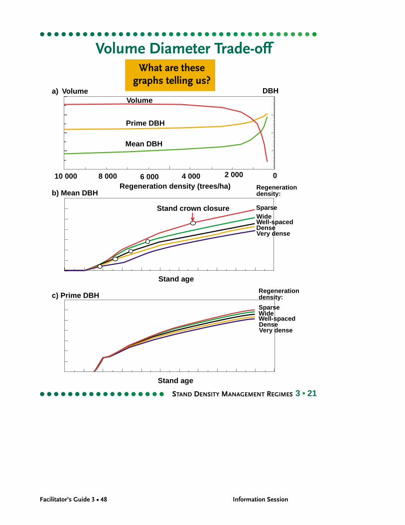
Volume Diameter Trade-off
Mean DBH
Prime DBH
Volume
Stand crown closure
a) Volume DBH
06 00010 000Regeneration density (trees/ha)
b) Mean DBH
Stand age
c) Prime DBH
Stand age
WideSparse
Well-spaced
Very denseDense
8 000 4 000 2 000
What are thesegraphs telling us?
Regenerationdensity:
WideSparse
Well-spaced
Very denseDense
Regenerationdensity:
○
○
○
○
○
○
○
○
○
○
○
○
○
○
○
○
○
○
○
○
○
○
○
○
○
○
○
○
○
○
○
○
○
○
○
○
○
○
○
○
○
○
○
○
○
○
○
○
○
○
○
○
○
○
○
○
○
○
○
○
○
○
○
○
○
○
○
○
○
○
○
○
○
○
○
○
○
○
○
○
○
○
○
○
○
Developing Stand Density Management Regimes Facilitator’s Guide 3 • 49
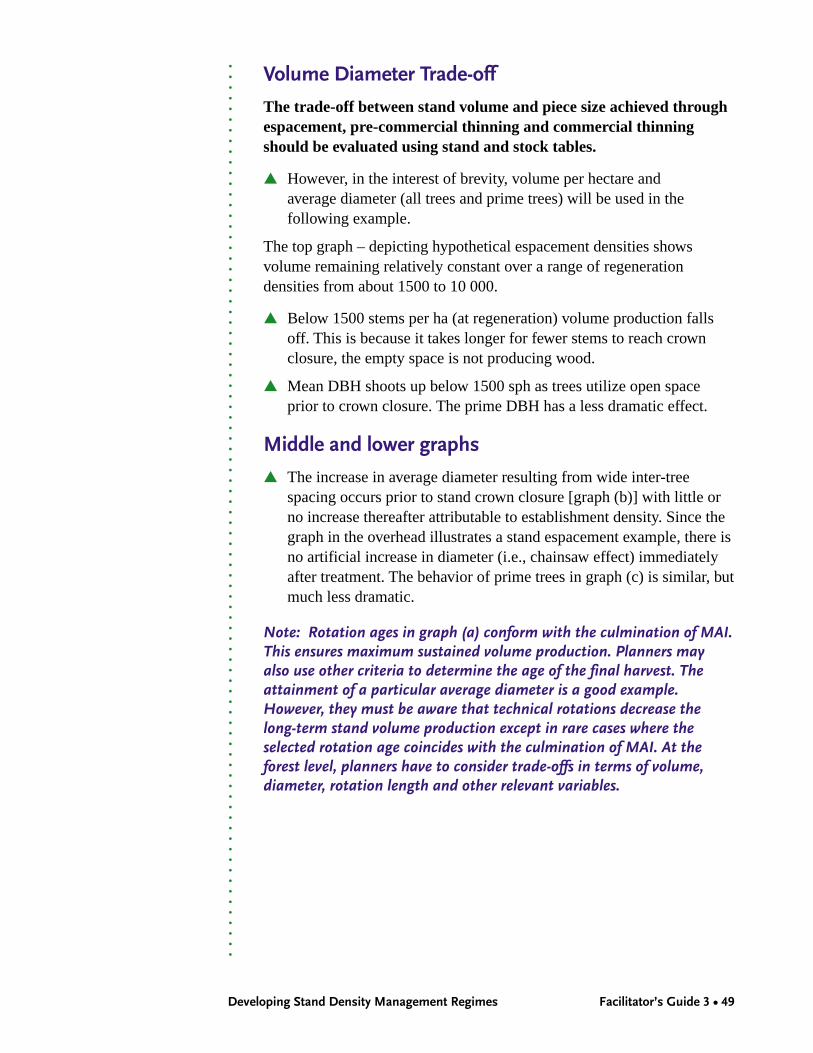
Volume Diameter Trade-off
The trade-off between stand volume and piece size achieved throughespacement, pre-commercial thinning and commercial thinningshould be evaluated using stand and stock tables.
▲ However, in the interest of brevity, volume per hectare andaverage diameter (all trees and prime trees) will be used in thefollowing example.
The top graph – depicting hypothetical espacement densities showsvolume remaining relatively constant over a range of regenerationdensities from about 1500 to 10 000.
▲ Below 1500 stems per ha (at regeneration) volume production fallsoff. This is because it takes longer for fewer stems to reach crownclosure, the empty space is not producing wood.
▲ Mean DBH shoots up below 1500 sph as trees utilize open spaceprior to crown closure. The prime DBH has a less dramatic effect.
Middle and lower graphs
▲ The increase in average diameter resulting from wide inter-treespacing occurs prior to stand crown closure [graph (b)] with little orno increase thereafter attributable to establishment density. Since thegraph in the overhead illustrates a stand espacement example, there isno artificial increase in diameter (i.e., chainsaw effect) immediatelyafter treatment. The behavior of prime trees in graph (c) is similar, butmuch less dramatic.
Note: Rotation ages in graph (a) conform with the culmination of MAI.This ensures maximum sustained volume production. Planners mayalso use other criteria to determine the age of the final harvest. Theattainment of a particular average diameter is a good example.However, they must be aware that technical rotations decrease thelong-term stand volume production except in rare cases where theselected rotation age coincides with the culmination of MAI. At theforest level, planners have to consider trade-offs in terms of volume,diameter, rotation length and other relevant variables.
Facilitator’s Guide 3 • 50 Information Session
Wood Quality
Stand density and itseffect on wood quality
3 • 22
Wood Quality – What is it?
▲ It depends on the end product
What attributes are important?
▲ Attractive visual features?
▲ Dimensional stability?
▲ Bracing strength?
▲ Strength and stiffness?
▲ Ring width
0 10 20 30 4 50 60 70Age
0.25
0.30
0.35
0.40
0.45
0.50
0.55
Relative density
Douglas-fir
W. hemlock
yellow cedarlodgepole
W. redcedar
interior spruceDistribution of juvenile
and mature wood
DBH (cm):
NarrowWideVerywide
54cm
Juvenile wood
Mature wood55% 48% 45%
59 54 51

○
○
○
○
○
○
○
○
○
○
○
○
○
○
○
○
○
○
○
○
○
○
○
○
○
○
○
○
○
○
○
○
○
○
○
○
○
○
○
○
○
○
○
○
○
○
○
○
○
○
○
○
○
○
○
○
○
○
○
○
○
○
○
○
○
○
○
○
○
○
○
○
○
○
○
○
○
○
○
○
○
○
○
○
○
Developing Stand Density Management Regimes Facilitator’s Guide 3 • 51
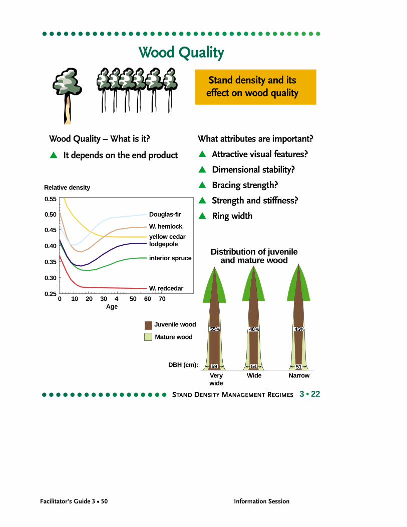
Wood Quality
The interactions between basic tree and wood properties and species,seed source, geographic location, site conditions and managementdecisions are very complex.
▲ As a result, it is difficult to discuss these relationships in detail.However, an attempt is made in this section to outline the moreimportant interactions in a general way so that foresters concernedwith maximizing timber value are aware that silviculture decisionscan affect both the tree volume and wood quality components oftimber value. Tree and wood quality refers to specific characteristicsthat affect the value recovery chain from harvesting of trees tomanufacturing and grade recovery of specific products (Zhang 1997).
Wood quality characteristics depend on the intended products and areusually defined by relative wood density, ring width, microfibril angle,fibre length, knot size and distribution, spiral grain angle and chemicalcomposition (e.g., lignin-cellulose ratios and extractives). Their affect onproduct quality and value have been discussed in detail by Jozsa andMiddleton (1994).
The key issues that can be affected by treatment are:
▲ Juvenile wood vs mature wood – Juvenile wood is crown derived(and often less dense – see figure 12 in the guidelines). Thus thelarger the crown the more juvenile wood. Wider spacing will result inmore juvenile wood in each stem (e.g., 55% vs 45% in the example),but how much will depend on the species and spacing density and thetime until harvest.
▲ Knot abundance and size – Will affect end use possibilities. Widespacing will produce larger knots limiting the end products insome cases (e.g., strength and appearance).
▲ Appearance – ring width and consistency. Heavy entries will resultin wide variation on ring width and could affect the esthetics ofthe product.
For more detailed information read A discussion of wood qualityattributes and their practical implications by L. Jozsa andG.R. Middleton, 1994, Special Publication SP-34 (as suggested in theguidelines).
Facilitator’s Guide 3 • 52 Information Session
Density and Other Factors
Other Factorsto Consider
3 • 23
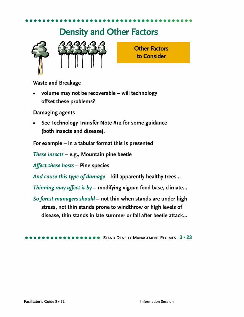
Waste and Breakage
• volume may not be recoverable – will technology
offset these problems?
Damaging agents
• See Technology Transfer Note #12 for some guidance
(both insects and disease).
For example – in a tabular format this is presented
These insects – e.g., Mountain pine beetle
Affect these hosts – Pine species
And cause this type of damage – kill apparently healthy trees…
Thinning may affect it by – modifying vigour, food base, climate…
So forest managers should – not thin when stands are under high
stress, not thin stands prone to windthrow or high levels of
disease, thin stands in late summer or fall after beetle attack…
○
○
○
○
○
○
○
○
○
○
○
○
○
○
○
○
○
○
○
○
○
○
○
○
○
○
○
○
○
○
○
○
○
○
○
○
○
○
○
○
○
○
○
○
○
○
○
○
○
○
○
○
○
○
○
○
○
○
○
○
○
○
○
○
○
○
○
○
○
○
○
○
○
○
○
○
○
○
○
○
○
○
○
○
○
Developing Stand Density Management Regimes Facilitator’s Guide 3 • 53
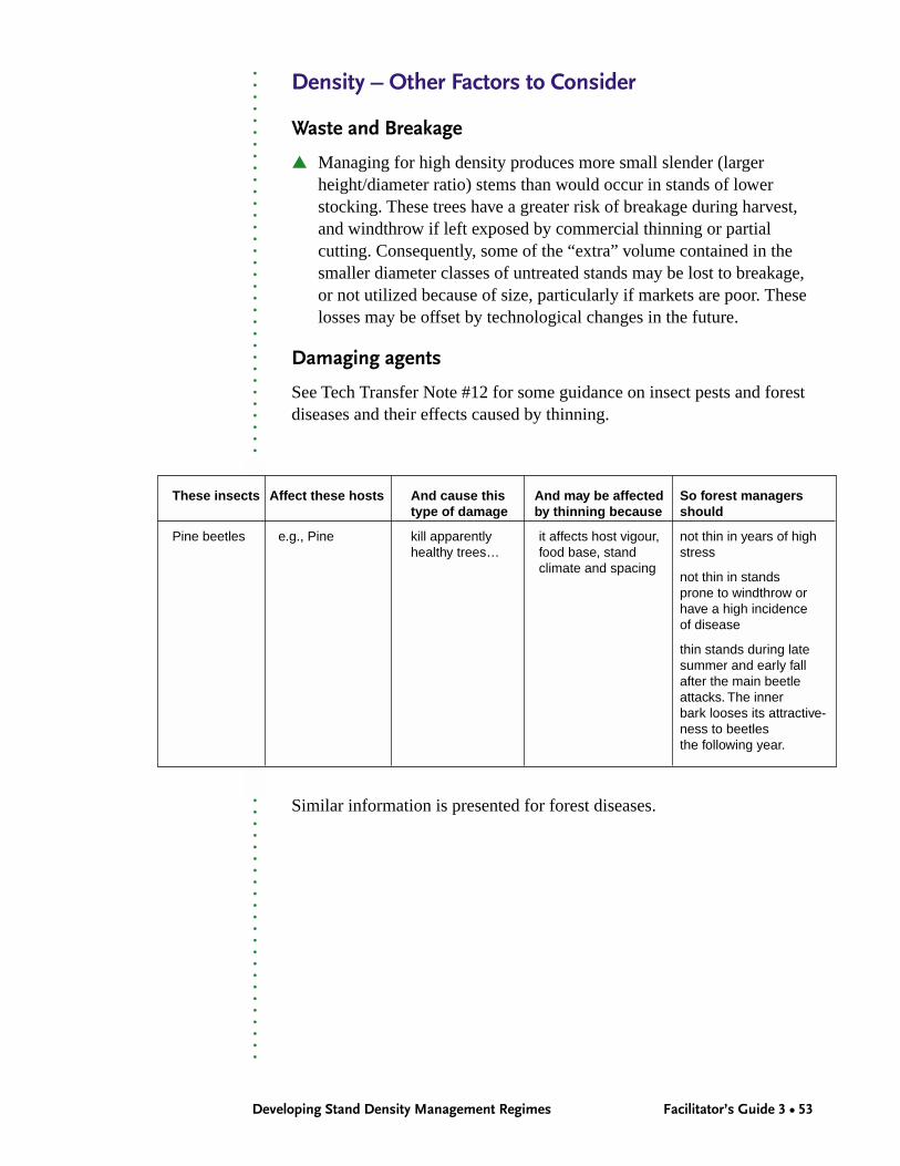
Density – Other Factors to Consider
Waste and Breakage
▲ Managing for high density produces more small slender (largerheight/diameter ratio) stems than would occur in stands of lowerstocking. These trees have a greater risk of breakage during harvest,and windthrow if left exposed by commercial thinning or partialcutting. Consequently, some of the “extra” volume contained in thesmaller diameter classes of untreated stands may be lost to breakage,or not utilized because of size, particularly if markets are poor. Theselosses may be offset by technological changes in the future.
Damaging agents
See Tech Transfer Note #12 for some guidance on insect pests and forestdiseases and their effects caused by thinning.
These insects Affect these hosts And cause this And may be affected So forest managerstype of damage by thinning because should
Pine beetles e.g., Pine kill apparently it affects host vigour, not thin in years of highhealthy trees… food base, stand stress
climate and spacingnot thin in standsprone to windthrow orhave a high incidenceof disease
thin stands during latesummer and early fallafter the main beetleattacks. The innerbark looses its attractive-ness to beetlesthe following year.
Similar information is presented for forest diseases.

Facilitator’s Guide 3 • 54 Information Session
Density and Other Factors
Other Factorsto Consider
3 • 24
Wildlife habitat
Spacing can increase or decreasehabitat values for different species.
For example:
Habitat quality Habitit quality Habitat qualitydecreased unaffected improved
Marten Gray wolf Coyote
Fisher Grizzly bear Black bear
Lynx Ermine Long-tailed weasel
Cougar
Bobcat
(From: Stand Tending Impacts on Environmental Indicators, 1996)
○
○
○
○
○
○
○
○
○
○
○
○
○
○
○
○
○
○
○
○
○
○
○
○
○
○
○
○
○
○
○
○
○
○
○
○
○
○
○
○
○
○
○
○
○
○
○
○
○
○
○
○
○
○
○
○
○
○
○
○
○
○
○
○
○
○
○
○
○
○
○
○
○
○
○
○
○
○
○
○
○
○
○
○
○
Developing Stand Density Management Regimes Facilitator’s Guide 3 • 55
Density – Other Factors to Consider
Wildlife habitat
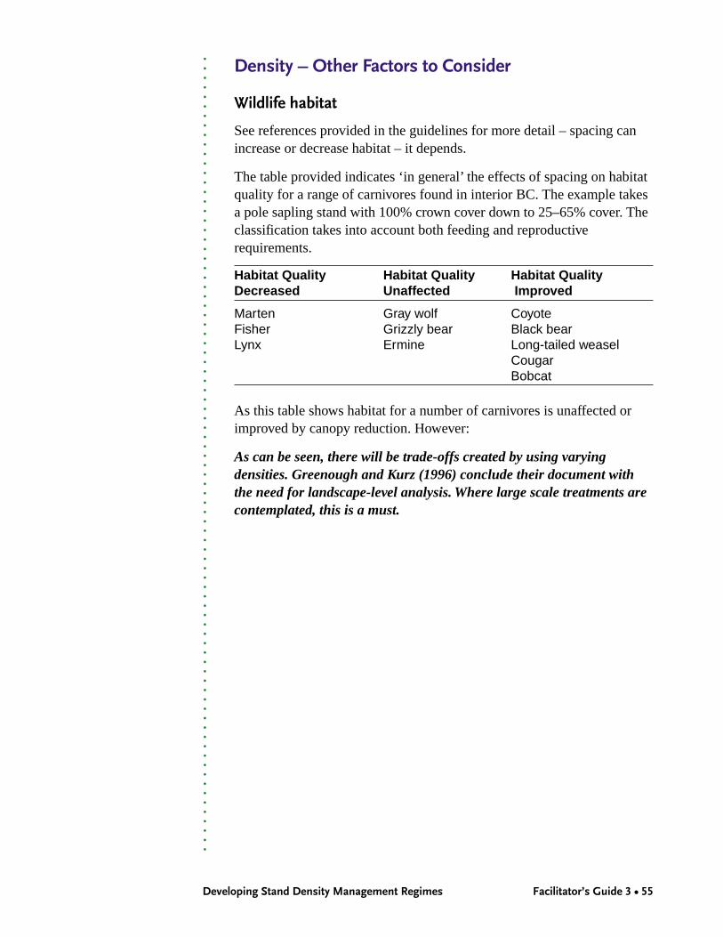
See references provided in the guidelines for more detail – spacing canincrease or decrease habitat – it depends.
The table provided indicates ‘in general’ the effects of spacing on habitatquality for a range of carnivores found in interior BC. The example takesa pole sapling stand with 100% crown cover down to 25–65% cover. Theclassification takes into account both feeding and reproductiverequirements.
Habitat Quality Habitat Quality Habitat QualityDecreased Unaffected Improved
Marten Gray wolf CoyoteFisher Grizzly bear Black bearLynx Ermine Long-tailed weasel
CougarBobcat
As this table shows habitat for a number of carnivores is unaffected orimproved by canopy reduction. However:
As can be seen, there will be trade-offs created by using varyingdensities. Greenough and Kurz (1996) conclude their document withthe need for landscape-level analysis. Where large scale treatments arecontemplated, this is a must.
Facilitator’s Guide 3 • 56 Information Session
Density and Other Factors
Other Factorsto Consider
3 • 25
Hydrology
▲ No effects of thinning identified to date.
Biotic and abiotic effects of spacing – ?
▲ more rapid decomposition
▲ possibly more respiration…
▲ more rapid movement of root decay inoculum
IN CONCLUSION...
BEWARE: Spacing can result in positive and negativeconsequences.
You should be aware of the possibilities before you start.
○
○
○
○
○
○
○
○
○
○
○
○
○
○
○
○
○
○
○
○
○
○
○
○
○
○
○
○
○
○
○
○
○
○
○
○
○
○
○
○
○
○
○
○
○
○
○
○
○
○
○
○
○
○
○
○
○
○
○
○
○
○
○
○
○
○
○
○
○
○
○
○
○
○
○
○
○
○
○
○
○
○
○
○
○
Developing Stand Density Management Regimes Facilitator’s Guide 3 • 57
Density – Other Factors to Consider
Hydrology
No effects of thinning identified to date. The key is – likely time untilcrown closure. If this is affected dramatically (e.g., very wide or clumpyspacing) the recovery rate may be significantly reduced. Present densityreductions have not been shown to affect hydrological recovery rate.
Biotic and abiotic effects of spacing
Many site and stand factors may be affected by stand densitymanagement practices; some may enhance the productive capacity of thestand, while others may introduce elements of uncertainty and risk.For instance:
▲ Higher levels of sunlight and warmer soil temperature may influencemicro-organisms and the rate of nutrient cycling.
▲ Increased micro-organism activity may increase the decompositionrates of slash remaining after thinning, and eventually improvemineral nutrient availability for the remaining crop trees.
▲ Reduced uptake by the stand may influence the diurnal and seasonalavailability of soil moisture, thereby influencing the pattern ofstomatal activity, duration of photosynthesis, and the rate of biomassproduction in the standing crop.
▲ Increased sunlight, warmer air temperatures and increased airmovement may increase the respiration rate of the standing crop,partially offsetting increased biomass production rates.
▲ Cutting activity associated with thinning may increase theconcentration and spread of root decay inoculum within the stand,resulting in greater losses of usable timber from the stand.
The characteristics of the site and stand may indicate the potentialsignificance of these biotic and abiotic responses to density managementdecision making.
In Conclusion...
Beware – spacing can result in positiveand negative consequences.
You should be aware of the possibilitiesbefore you start.
As a parting word on biology and spacing effects – spacing is crown andgap management to achieve a desired result. Stay informed.

Recommended