Lecture 5: Value Function Approximation
Emma Brunskill
CS234 Reinforcement Learning.
Winter 2018
The value function approximation structure for today closely follows muchof David Silver’s Lecture 6. For additional reading please see SB 2018Sections 9.3, 9.6-9.7. The deep learning slides come almost exclusivelyfrom Ruslan Salakhutdinov’s class, and Hugo Larochelle’s class (and withthanks to Zico Kolter also for slide inspiration). The slides in my standardstyle format in the deep learning section are my own.
Emma Brunskill (CS234 Reinforcement Learning. )Lecture 5: Value Function Approximation Winter 2018 1 / 48

Important Information About Homework 2
Homework 2 will now be due on Saturday February 10 (instead ofFebruary 7)
We are making this change to try to give some background on deeplearning, give people enough time to do homework 2, and still givepeople time to study for the midterm on February 14
We will release the homework this week
You will be able to start on some aspects of the homework this week,but we will be covering DQN which is the largest part, on Monday
We will also be providing optional tutorial sessions on tensorflow
Emma Brunskill (CS234 Reinforcement Learning. )Lecture 5: Value Function Approximation Winter 2018 2 / 48
Table of Contents
1 Introduction
2 VFA for Prediction
3 Control using Value Function Approximation
4 Deep Learning
Emma Brunskill (CS234 Reinforcement Learning. )Lecture 5: Value Function Approximation Winter 2018 3 / 48
Class Structure
Last time: Control (making decisions) without a model of how theworld works
This time: Value function approximation and deep learning
Next time: Deep reinforcement learning
Emma Brunskill (CS234 Reinforcement Learning. )Lecture 5: Value Function Approximation Winter 2018 4 / 48

Last time: Model-Free Control
Last time: how to learn a good policy from experience
So far, have been assuming we can represent the value function orstate-action value function as a vector
Tabular representation
Many real world problems have enormous state and/or action spaces
Tabular representation is insu�cient
Emma Brunskill (CS234 Reinforcement Learning. )Lecture 5: Value Function Approximation Winter 2018 5 / 48
Recall: Reinforcement Learning Involves
Optimization
Delayed consequences
Exploration
Generalization
Emma Brunskill (CS234 Reinforcement Learning. )Lecture 5: Value Function Approximation Winter 2018 6 / 48

Today: Focus on Generalization
Optimization
Delayed consequences
Exploration
Generalization
Emma Brunskill (CS234 Reinforcement Learning. )Lecture 5: Value Function Approximation Winter 2018 7 / 48

Table of Contents
1 Introduction
2 VFA for Prediction
3 Control using Value Function Approximation
4 Deep Learning
Emma Brunskill (CS234 Reinforcement Learning. )Lecture 5: Value Function Approximation Winter 2018 8 / 48

Value Function Approximation (VFA)
Represent a (state-action/state) value function with a parameterizedfunction instead of a table
Emma Brunskill (CS234 Reinforcement Learning. )Lecture 5: Value Function Approximation Winter 2018 9 / 48

Motivation for VFA
Don’t want to have to explicitly store or learn for every single state aDynamics or reward modelValueState-action valuePolicy
Want more compact representation that generalizes across state orstates and actions
Emma Brunskill (CS234 Reinforcement Learning. )Lecture 5: Value Function Approximation Winter 2018 10 / 48
Benefits of Generalization
Reduce memory needed to store (P ,R)/V /Q/⇡
Reduce computation needed to compute (P ,R)/V /Q/⇡
Reduce experience needed to find a good P ,R/V /Q/⇡
Emma Brunskill (CS234 Reinforcement Learning. )Lecture 5: Value Function Approximation Winter 2018 11 / 48

Value Function Approximation (VFA)
Represent a (state-action/state) value function with a parameterizedfunction instead of a table
Which function approximator?
Emma Brunskill (CS234 Reinforcement Learning. )Lecture 5: Value Function Approximation Winter 2018 12 / 48

Function Approximators
Many possible function approximators includingLinear combinations of featuresNeural networksDecision treesNearest neighborsFourier / wavelet bases
In this class we will focus on function approximators that aredi↵erentiable (Why?)
Two very popular classes of di↵erentiable function approximatorsLinear feature representations (Today)Neural networks (Today and next lecture)
Emma Brunskill (CS234 Reinforcement Learning. )Lecture 5: Value Function Approximation Winter 2018 13 / 48
Review: Gradient Descent
Consider a function J(w) that is a di↵erentiable function of aparameter vector w
Goal is to find parameter w that minimizes J
The gradient of J(w) is
Emma Brunskill (CS234 Reinforcement Learning. )Lecture 5: Value Function Approximation Winter 2018 14 / 48

Table of Contents
1 Introduction
2 VFA for Prediction
3 Control using Value Function Approximation
4 Deep Learning
Emma Brunskill (CS234 Reinforcement Learning. )Lecture 5: Value Function Approximation Winter 2018 15 / 48
Value Function Approximation for Policy Evaluation withan Oracle
First consider if could query any state s and an oracle would returnthe true value for v⇡(s)
The objective was to find the best approximate representation of v⇡
given a particular parameterized function
Emma Brunskill (CS234 Reinforcement Learning. )Lecture 5: Value Function Approximation Winter 2018 16 / 48

Stochastic Gradient Descent
Goal: Find the parameter vector w that minimizes the loss between atrue value function v⇡(s) and its approximation v as represented witha particular function class parameterized by w .
Generally use mean squared error and define the loss as
J(w) = ⇡[(v⇡(S)� v(S ,w))2] (1)
Can use gradient descent to find a local minimum
�w = �1
2↵5w J(w) (2)
Stochastic gradient descent (SGD) samples the gradient:
Expected SGD is the same as the full gradient update
Emma Brunskill (CS234 Reinforcement Learning. )Lecture 5: Value Function Approximation Winter 2018 17 / 48
VFA Prediction Without An Oracle
Don’t actually have access to an oracle to tell true v⇡(S) for anystate s
Now consider how to do value function approximation for prediction /evaluation / policy evaluation without a model
Note: policy evaluation without a model is sometimes also calledpassive reinforcement learning with value function approximation
”passive” because not trying to learn the optimal decision policy
Emma Brunskill (CS234 Reinforcement Learning. )Lecture 5: Value Function Approximation Winter 2018 18 / 48
Model Free VFA Prediction / Policy Evaluation
Recall model-free policy evaluation (Lecture 3)Following a fixed policy ⇡ (or had access to prior data)Goal is to estimate V
⇡ and/or Q⇡
Maintained a look up table to store estimates V ⇡ and/or Q⇡
Updated these estimates after each episode (Monte Carlo methods)or after each step (TD methods)
Now: in value function approximation, change the estimateupdate step to include fitting the function approximator
Emma Brunskill (CS234 Reinforcement Learning. )Lecture 5: Value Function Approximation Winter 2018 19 / 48
Feature Vectors
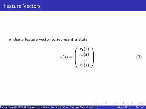
Use a feature vector to represent a state
x(s) =
0
BB@
x
1
(s)x
2
(s). . .xn(s)
1
CCA (3)
Emma Brunskill (CS234 Reinforcement Learning. )Lecture 5: Value Function Approximation Winter 2018 20 / 48
Linear Value Function Approximation for Prediction WithAn Oracle
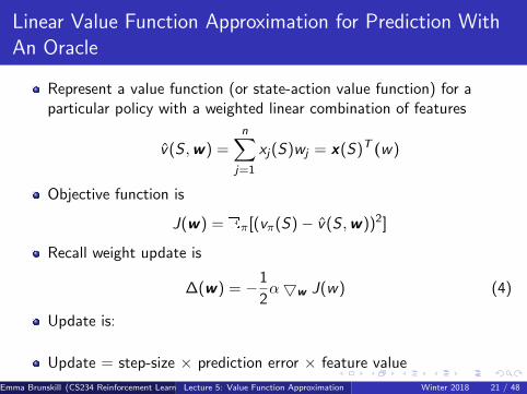
Represent a value function (or state-action value function) for aparticular policy with a weighted linear combination of features
v(S ,w) =nX
j=1
xj(S)wj = x(S)T (w)
Objective function is
J(w) = ⇡[(v⇡(S)� v(S ,w))2]
Recall weight update is
�(w) = �1
2↵5w J(w) (4)
Update is:
Update = step-size ⇥ prediction error ⇥ feature value
Emma Brunskill (CS234 Reinforcement Learning. )Lecture 5: Value Function Approximation Winter 2018 21 / 48

Monte Carlo Value Function Approximation
Return Gt is an unbiased but noisy sample of the true expected returnv⇡(St)
Therefore can reduce MC VFA to doing supervised learning on a setof (state,return) pairs: < S
1
,G1
>,< S
2
,G2
>, . . . , < ST ,GT >Susbstituting Gt(St) for the true v⇡(St) when fitting the functionapproximator
Concretely when using linear VFA for policy evaluation
�w = ↵(Gt � v(St ,w))5w v(St ,w) (5)
= ↵(Gt � v(St ,w))x(St) (6)
Note: Gt may be a very noisy estimate of true return
Emma Brunskill (CS234 Reinforcement Learning. )Lecture 5: Value Function Approximation Winter 2018 22 / 48

MC Linear Value Function Approximation for PolicyEvaluation
1: Initialize w = 0,Returns(s) = 0 8(s, a), k = 12: loop3: Sample k-th episode (sk1, ak1, rk1, sk2, . . . , sk,Lk ) given ⇡4: for t = 1, . . . , Lk do5: if First visit to (s) in episode k then6: Append
PLkj=t rkj to Returns(st)
7: Update weights
8: end if9: end for
10: k = k + 111: end loop
Emma Brunskill (CS234 Reinforcement Learning. )Lecture 5: Value Function Approximation Winter 2018 23 / 48

Recall: Temporal Di↵erence (TD(0)) Learning with a Lookup Table
Uses bootstrapping and sampling to approximate V
⇡
Updates V ⇡(s) after each transition (s, a, r , s 0):
V
⇡(s) = V
⇡(s) + ↵(r + �V ⇡(s 0)� V
⇡(s)) (7)
Target is r + �V ⇡(s 0), a biased estimate of the true value v
⇡(s)
Look up table represents value for each state with a separate tableentry
Emma Brunskill (CS234 Reinforcement Learning. )Lecture 5: Value Function Approximation Winter 2018 24 / 48

Temporal Di↵erence (TD(0)) Learning with ValueFunction Approximation
Uses bootstrapping and sampling to approximate true v
⇡
Updates estimate V
⇡(s) after each transition (s, a, r , s 0):
V
⇡(s) = V
⇡(s) + ↵(r + �V ⇡(s 0)� V
⇡(s)) (8)
Target is r + �V ⇡(s 0), a biased estimate of of the true value v
⇡(s)
In value function approximation, target is r + �v⇡(s 0), a biased andapproximated estimate of of the true value v
⇡(s)
3 forms of approximation:
Emma Brunskill (CS234 Reinforcement Learning. )Lecture 5: Value Function Approximation Winter 2018 25 / 48
Temporal Di↵erence (TD(0)) Learning with ValueFunction Approximation
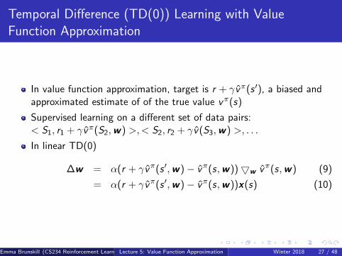
In value function approximation, target is r + �v⇡(s 0), a biased andapproximated estimate of of the true value v
⇡(s)
Supervised learning on a di↵erent set of data pairs:< S
1
, r1
+ �v⇡(S2
,w) >,< S
2
, r2
+ �v(S3
,w) >, . . .
Emma Brunskill (CS234 Reinforcement Learning. )Lecture 5: Value Function Approximation Winter 2018 26 / 48
Temporal Di↵erence (TD(0)) Learning with ValueFunction Approximation
In value function approximation, target is r + �v⇡(s 0), a biased andapproximated estimate of of the true value v
⇡(s)
Supervised learning on a di↵erent set of data pairs:< S
1
, r1
+ �v⇡(S2
,w) >,< S
2
, r2
+ �v(S3
,w) >, . . .
In linear TD(0)
�w = ↵(r + �v⇡(s 0,w)� v
⇡(s,w))5w v
⇡(s,w) (9)
= ↵(r + �v⇡(s 0,w)� v
⇡(s,w))x(s) (10)
Emma Brunskill (CS234 Reinforcement Learning. )Lecture 5: Value Function Approximation Winter 2018 27 / 48
Convergence Guarantees for Linear Value FunctionApproximation for Policy Evaluation1
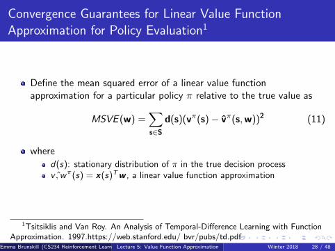
Define the mean squared error of a linear value functionapproximation for a particular policy ⇡ relative to the true value as
MSVE (w) =X
s2Sd(s)(v⇡(s)� v⇡(s,w))2 (11)
whered(s): stationary distribution of ⇡ in the true decision processˆv ,w⇡(s) = x(s)Tw , a linear value function approximation
1
Tsitsiklis and Van Roy. An Analysis of Temporal-Di↵erence Learning with Function
Approximation. 1997.https://web.stanford.edu/ bvr/pubs/td.pdf
Emma Brunskill (CS234 Reinforcement Learning. )Lecture 5: Value Function Approximation Winter 2018 28 / 48

Convergence Guarantees for Linear Value FunctionApproximation for Policy Evaluation2
Define the mean squared error of a linear value functionapproximation for a particular policy ⇡ relative to the true value as
MSVE (w) =X
s2Sd(s)(v⇡(s)� v⇡(s,w))2 (12)
whered(s): stationary distribution of ⇡ in the true decision processv
⇡(s) = x(s)Tw , a linear value function approximation
Monte Carlo policy evaluation with VFA converges to the weightswMC which has the minimum mean squared error possible:
MSVE (wMC ) = minw
X
s2Sd(s)(v⇡ ⇤ (s)� v
⇡(s,w))2 (13)
2
Tsitsiklis and Van Roy. An Analysis of Temporal-Di↵erence Learning with Function
Approximation. 1997.https://web.stanford.edu/ bvr/pubs/td.pdf
Emma Brunskill (CS234 Reinforcement Learning. )Lecture 5: Value Function Approximation Winter 2018 29 / 48
Convergence Guarantees for Linear Value FunctionApproximation for Policy Evaluation3
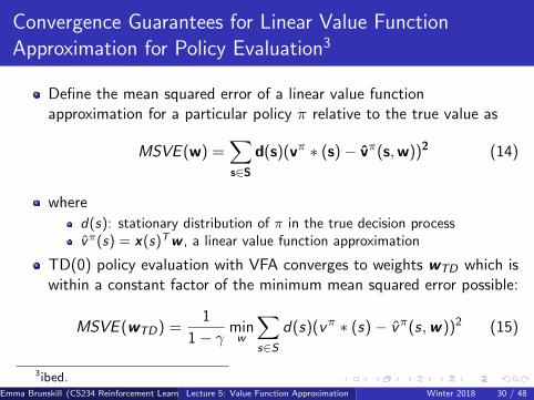
Define the mean squared error of a linear value functionapproximation for a particular policy ⇡ relative to the true value as
MSVE (w) =X
s2Sd(s)(v⇡ ⇤ (s)� v⇡(s,w))2 (14)
whered(s): stationary distribution of ⇡ in the true decision processv
⇡(s) = x(s)Tw , a linear value function approximation
TD(0) policy evaluation with VFA converges to weights wTD which iswithin a constant factor of the minimum mean squared error possible:
MSVE (wTD) =1
1� �minw
X
s2Sd(s)(v⇡ ⇤ (s)� v
⇡(s,w))2 (15)
3
ibed.
Emma Brunskill (CS234 Reinforcement Learning. )Lecture 5: Value Function Approximation Winter 2018 30 / 48

Summary: Convergence Guarantees for Linear ValueFunction Approximation for Policy Evaluation4
Monte Carlo policy evaluation with VFA converges to the weightswMC which has the minimum mean squared error possible:
MSVE (wMC ) = minw
X
s2Sd(s)(v⇡ ⇤ (s)� v
⇡(s,w))2 (16)
TD(0) policy evaluation with VFA converges to weights wTD which iswithin a constant factor of the minimum mean squared error possible:
MSVE (wTD) =1
1� �minw
X
s2Sd(s)(v⇡ ⇤ (s)� v
⇡(s,w))2 (17)
Check your understanding: if the VFA is a tabular representation (onefeature for each state), what is the MSVE for MC and TD?
4
ibed.
Emma Brunskill (CS234 Reinforcement Learning. )Lecture 5: Value Function Approximation Winter 2018 31 / 48
Convergence Rates for Linear Value FunctionApproximation for Policy Evaluation
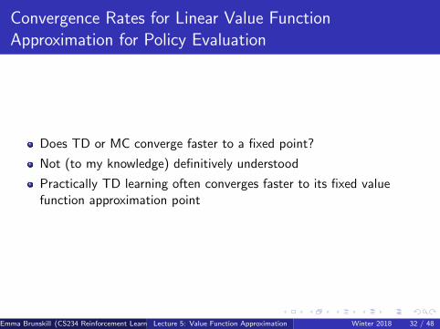
Does TD or MC converge faster to a fixed point?
Not (to my knowledge) definitively understood
Practically TD learning often converges faster to its fixed valuefunction approximation point
Emma Brunskill (CS234 Reinforcement Learning. )Lecture 5: Value Function Approximation Winter 2018 32 / 48

Table of Contents
1 Introduction
2 VFA for Prediction
3 Control using Value Function Approximation
4 Deep Learning
Emma Brunskill (CS234 Reinforcement Learning. )Lecture 5: Value Function Approximation Winter 2018 33 / 48

Control using Value Function Approximation
Use value function approximation to represent state-action valuesq
⇡(s, a,w) ⇡ q
⇡
InterleaveApproximate policy evaluation using value function approximationPerform ✏-greedy policy improvement
Emma Brunskill (CS234 Reinforcement Learning. )Lecture 5: Value Function Approximation Winter 2018 34 / 48

Action-Value Function Approximation with an Oracle
q
⇡(s, a,w) ⇡ q
⇡
Minimize the mean-squared error between the true action-valuefunction q
⇡(s, a) and the approximate action-value function:
J(w) = ⇡[(q⇡(s, a)� q
⇡(s, a,w))2] (18)
Use stochastic gradient descent to find a local minimum
�1
25W J(w) = [(q⇡(s, a)� q
⇡(s, a,w))5w q
⇡(s, a,w)](19)
�(w) = �1
2↵5w J(w) (20)
Stochastic gradient descent (SGD) samples the gradient
Emma Brunskill (CS234 Reinforcement Learning. )Lecture 5: Value Function Approximation Winter 2018 35 / 48

Linear State Action Value Function Approximation with anOracle
Use features to represent both the state and action
x(s, a) =
0
BB@
x
1
(s, a)x
2
(s, a). . .
xn(s, a)
1
CCA (21)
Represent state-action value function with a weighted linearcombination of features
q(s, a,w) = x(s, a)Tw =nX
j=1
xj(s, a)wj (22)
Stochastic gradient descent update:
5wJ(w) = 5w ⇡[(q⇡(s, a)� q
⇡(s, a,w))2] (23)
Emma Brunskill (CS234 Reinforcement Learning. )Lecture 5: Value Function Approximation Winter 2018 36 / 48
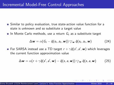
Incremental Model-Free Control Approaches
Similar to policy evaluation, true state-action value function for astate is unknown and so substitute a target value
In Monte Carlo methods, use a return Gt as a substitute target
�w = ↵(Gt � q(st , at ,w))5w q(st , at ,w) (24)
For SARSA instead use a TD target r + �q(s 0, a0,w) which leveragesthe current function approximation value
�w = ↵(r + �q(s 0, a0,w)� q(s, a,w))5w q(s, a,w) (25)
Emma Brunskill (CS234 Reinforcement Learning. )Lecture 5: Value Function Approximation Winter 2018 37 / 48

Incremental Model-Free Control Approaches
Similar to policy evaluation, true state-action value function for astate is unknown and so substitute a target value
In Monte Carlo methods, use a return Gt as a substitute target
�w = ↵(Gt � q(st , at ,w))5w q(st , at ,w) (26)
For SARSA instead use a TD target r + �q(s 0, a0,w) which leveragesthe current function approximation value
�w = ↵(r + �q(s 0, a0,w)� q(s, a,w))5w q(s, a,w) (27)
For Q-learning instead use a TD target r + �maxa q(s 0, a0,w) whichleverages the max of the current function approximation value
�w = ↵(r + �maxa0
q(s 0, a0,w)� q(s, a,w))5w q(s, a,w) (28)
Emma Brunskill (CS234 Reinforcement Learning. )Lecture 5: Value Function Approximation Winter 2018 38 / 48

Convergence of TD Methods with VFA
TD with value function approximation is not following the gradient ofan objective function
Informally, updates involve doing an (approximate) Bellman backupfollowed by best trying to fit underlying value function to a particularfeature representation
Bellman operators are contractions, but value function approximationfitting can be an expansion
Emma Brunskill (CS234 Reinforcement Learning. )Lecture 5: Value Function Approximation Winter 2018 39 / 48

Convergence of Control Methods with VFA
Algorithm Tabular Linear VFA Nonlinear VFAMonte-Carlo Control
SarsaQ-learning
Emma Brunskill (CS234 Reinforcement Learning. )Lecture 5: Value Function Approximation Winter 2018 40 / 48

Table of Contents
1 Introduction
2 VFA for Prediction
3 Control using Value Function Approximation
4 Deep Learning
Emma Brunskill (CS234 Reinforcement Learning. )Lecture 5: Value Function Approximation Winter 2018 41 / 48

Other Function Approximators
Linear value function approximators often work well given the rightset of features
But can require carefully hand designing that feature set
An alternative is to use a much richer function approximation classthat is able to directly go from states without requiring an explicitspecification of features
Local representations including Kernel based approaches have someappealing properties (including convergence results under certaincases) but can’t typically scale well to enormous spaces and datasets
Alternative is to leverage huge recent success in using deep neuralnetworks
Emma Brunskill (CS234 Reinforcement Learning. )Lecture 5: Value Function Approximation Winter 2018 42 / 48
Deep Neural Networks
Today: a brief introduction to deep neural networks
Definitions
Power of deep neural networksNeural networks / distributed representations vs kernel / localrepresentationsUniversal function approximatorDeep neural networks vs shallow neural networks
How to train neural nets
Emma Brunskill (CS234 Reinforcement Learning. )Lecture 5: Value Function Approximation Winter 2018 43 / 48

Deep Neural Networks
Today: a brief introduction to deep neural networks
Definitions
Power of deep neural networksNeural networks / distributed representations vs kernel / localrepresentationsUniversal function approximatorDeep neural networks vs shallow neural networks
How to train neural nets
Emma Brunskill (CS234 Reinforcement Learning. )Lecture 5: Value Function Approximation Winter 2018 44 / 48

Deep Neural Networks
Today: a brief introduction to deep neural networks
Definitions
Power of deep neural networksNeural networks / distributed representations vs kernel / localrepresentationsUniversal function approximatorDeep neural networks vs shallow neural networks
How to train neural nets
Emma Brunskill (CS234 Reinforcement Learning. )Lecture 5: Value Function Approximation Winter 2018 45 / 48

Deep Learning

Deep Neural Networks
Today: a brief introduction to deep neural networks
Definitions
Power of deep neural networksNeural networks / distributed representations vs kernel / localrepresentationsUniversal function approximatorDeep neural networks vs shallow neural networks
How to train neural nets
Emma Brunskill (CS234 Reinforcement Learning. )Lecture 5: Value Function Approximation Winter 2018 46 / 48

Feedforward Neural Networks ‣ Definition of Neural Networks
- Forward propagation - Types of units - Capacity of neural networks
‣ How to train neural nets: - Loss function - Backpropagation with gradient descent
‣ More recent techniques: - Dropout - Batch normalization - Unsupervised Pre-training
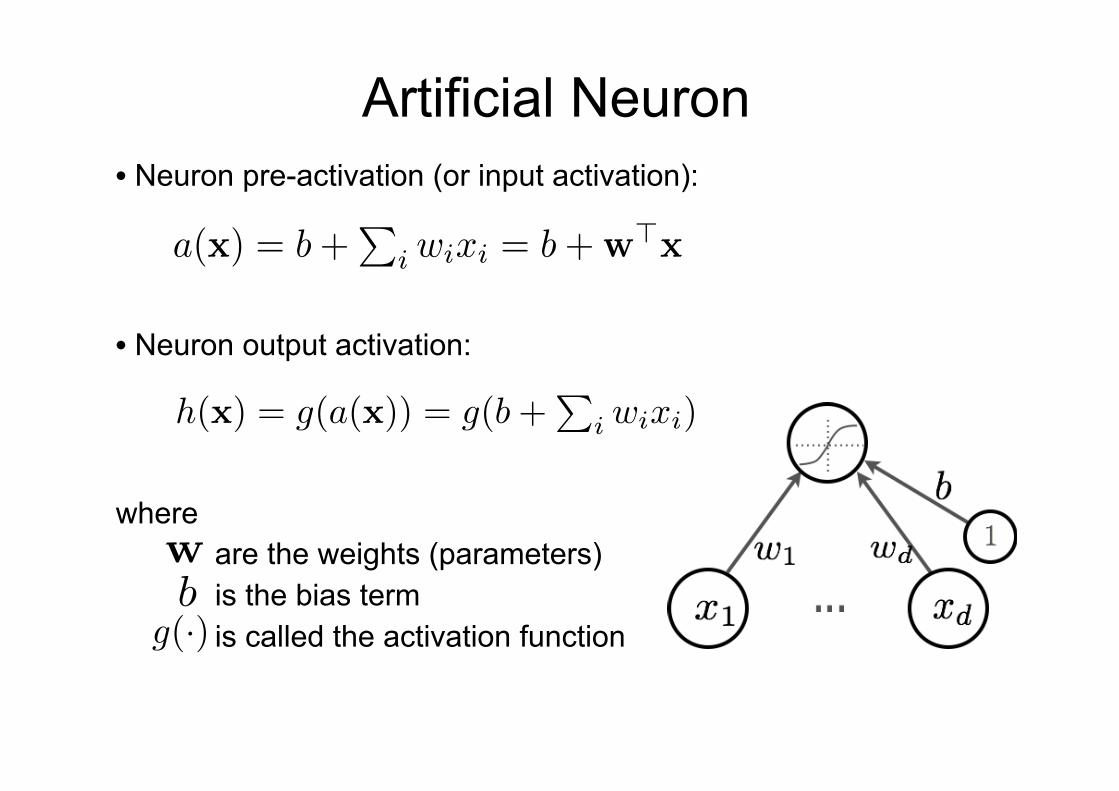
Artificial Neuron • Neuron pre-activation (or input activation):
Feedforward neural network
Hugo LarochelleD
´
epartement d’informatique
Universit
´
e de Sherbrooke
September 6, 2012
Abstract
Math for my slides “Feedforward neural network”.
• a(x) = b+P
i wixi = b+w
>x
• h(x) = g(a(x)) = g(b+P
i wixi)
• x
1
xd b w
1
wd
• w
• {
• g(·) b
• h(x) = g(a(x))
• a(x) = b
(1) +W
(1)
x
⇣a(x)i = b
(1)
i
Pj W
(1)
i,j xj
⌘
• o(x) = g
(out)(b(2) +w
(2)
>x)
1
• Neuron output activation:
Feedforward neural network
Hugo LarochelleD
´
epartement d’informatique
Universit
´
e de Sherbrooke
September 6, 2012
Abstract
Math for my slides “Feedforward neural network”.
• a(x) = b+P
i wixi = b+w
>x
• h(x) = g(a(x)) = g(b+P
i wixi)
• x
1
xd b w
1
wd
• w
• {
• g(·) b
• h(x) = g(a(x))
• a(x) = b
(1) +W
(1)
x
⇣a(x)i = b
(1)
i
Pj W
(1)
i,j xj
⌘
• o(x) = g
(out)(b(2) +w
(2)
>x)
1
where are the weights (parameters) is the bias term is called the activation function
Feedforward neural network
Hugo LarochelleD
´
epartement d’informatique
Universit
´
e de Sherbrooke
September 6, 2012
Abstract
Math for my slides “Feedforward neural network”.
• a(x) = b+P
i wixi = b+w
>x
• h(x) = g(a(x)) = g(b+P
i wixi)
• x
1
xd b w
1
wd
• w
• {
• g(·) b
• h(x) = g(a(x))
• a(x) = b
(1) +W
(1)
x
⇣a(x)i = b
(1)
i
Pj W
(1)
i,j xj
⌘
• o(x) = g
(out)(b(2) +w
(2)
>x)
1
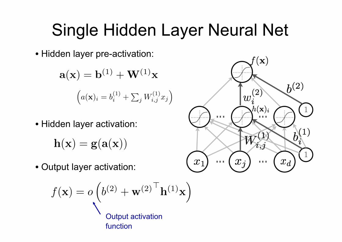
Single Hidden Layer Neural Net • Hidden layer pre-activation:
Feedforward neural network
Hugo LarochelleD
´
epartement d’informatique
Universit
´
e de Sherbrooke
September 6, 2012
Abstract
Math for my slides “Feedforward neural network”.
• a(x) = b+
Pi wixi = b+w
>x
• h(x) = g(a(x)) = g(b+
Pi wixi)
• x
1
xd b w
1
wd
• w
• {
• g(a) = a
• g(a) = sigm(a) =
1
1+exp(�a)
• g(a) = tanh(a) =
exp(a)�exp(�a)exp(a)+exp(�a) =
exp(2a)�1
exp(2a)+1
• g(a) = max(0, a)
• g(a) = reclin(a) = max(0, a)
• g(·) b
• W
(1)
i,j b
(1)
i xj h(x)i w
(2)
i b
(2)
• h(x) = g(a(x))
• a(x) = b
(1)
+W
(1)
x
⇣a(x)i = b
(1)
i +
Pj W
(1)
i,j xj
⌘
• f(x) = o(b
(2)
+w
(2)
>x)
1
Feedforward neural network
Hugo LarochelleD
´
epartement d’informatique
Universit
´
e de Sherbrooke
September 6, 2012
Abstract
Math for my slides “Feedforward neural network”.
• a(x) = b+
Pi wixi = b+w
>x
• h(x) = g(a(x)) = g(b+
Pi wixi)
• x
1
xd b w
1
wd
• w
• {
• g(a) = a
• g(a) = sigm(a) =
1
1+exp(�a)
• g(a) = tanh(a) =
exp(a)�exp(�a)exp(a)+exp(�a) =
exp(2a)�1
exp(2a)+1
• g(a) = max(0, a)
• g(a) = reclin(a) = max(0, a)
• p(y = 1|x)
• g(·) b
• W
(1)
i,j b
(1)
i xj h(x)i w
(2)
i b
(2)
• h(x) = g(a(x))
• a(x) = b
(1)
+W
(1)
x
⇣a(x)i = b
(1)
i +
Pj W
(1)
i,j xj
⌘
• f(x) = o
⇣b
(2)
+w
(2)
>x
⌘
1
• Hidden layer activation:
Feedforward neural network
Hugo LarochelleD
´
epartement d’informatique
Universit
´
e de Sherbrooke
September 7, 2012
Abstract
Math for my slides “Feedforward neural network”.
• a(x) = b+
Pi wixi = b+w
>x
• h(x) = g(a(x)) = g(b+
Pi wixi)
• x
1
xd b w
1
wd
• w
• {
• g(a) = a
• g(a) = sigm(a) =
1
1+exp(�a)
• g(a) = tanh(a) =
exp(a)�exp(�a)exp(a)+exp(�a) =
exp(2a)�1
exp(2a)+1
• g(a) = max(0, a)
• g(a) = reclin(a) = max(0, a)
• p(y = 1|x)
• g(·) b
• W
(1)
i,j b
(1)
i xj h(x)i w
(2)
i b
(2)
• h(x) = g(a(x))
• a(x) = b
(1)
+W
(1)
x
⇣a(x)i = b
(1)
i +
Pj W
(1)
i,j xj
⌘
• f(x) = o
⇣b
(2)
+w
(2)
>h
(1)
x
⌘
1
• Output layer activation:
Output activation function

Artificial Neuron
Bias only changes the position of the riff
Range is determined by
Feedforward neural network
Hugo LarochelleD
´
epartement d’informatique
Universit
´
e de Sherbrooke
September 6, 2012
Abstract
Math for my slides “Feedforward neural network”.
• a(x) = b+P
i wixi = b+w
>x
• h(x) = g(a(x)) = g(b+P
i wixi)
• x
1
xd b w
1
wd
• w
• {
• g(·) b
• h(x) = g(a(x))
• a(x) = b
(1) +W
(1)
x
⇣a(x)i = b
(1)
i
Pj W
(1)
i,j xj
⌘
• o(x) = g
(out)(b(2) +w
(2)
>x)
1
• Output activation of the neuron:
Feedforward neural network
Hugo LarochelleD
´
epartement d’informatique
Universit
´
e de Sherbrooke
September 6, 2012
Abstract
Math for my slides “Feedforward neural network”.
• a(x) = b+P
i wixi = b+w
>x
• h(x) = g(a(x)) = g(b+P
i wixi)
• x
1
xd b w
1
wd
• w
• {
• g(·) b
• h(x) = g(a(x))
• a(x) = b
(1) +W
(1)
x
⇣a(x)i = b
(1)
i
Pj W
(1)
i,j xj
⌘
• o(x) = g
(out)(b(2) +w
(2)
>x)
1
(from Pascal Vincent’s slides)

Single Hidden Layer Neural Net • Hidden layer pre-activation:
Feedforward neural network
Hugo LarochelleD
´
epartement d’informatique
Universit
´
e de Sherbrooke
September 6, 2012
Abstract
Math for my slides “Feedforward neural network”.
• a(x) = b+
Pi wixi = b+w
>x
• h(x) = g(a(x)) = g(b+
Pi wixi)
• x
1
xd b w
1
wd
• w
• {
• g(a) = a
• g(a) = sigm(a) =
1
1+exp(�a)
• g(a) = tanh(a) =
exp(a)�exp(�a)exp(a)+exp(�a) =
exp(2a)�1
exp(2a)+1
• g(a) = max(0, a)
• g(a) = reclin(a) = max(0, a)
• g(·) b
• W
(1)
i,j b
(1)
i xj h(x)i w
(2)
i b
(2)
• h(x) = g(a(x))
• a(x) = b
(1)
+W
(1)
x
⇣a(x)i = b
(1)
i +
Pj W
(1)
i,j xj
⌘
• f(x) = o(b
(2)
+w
(2)
>x)
1
Feedforward neural network
Hugo LarochelleD
´
epartement d’informatique
Universit
´
e de Sherbrooke
September 6, 2012
Abstract
Math for my slides “Feedforward neural network”.
• a(x) = b+
Pi wixi = b+w
>x
• h(x) = g(a(x)) = g(b+
Pi wixi)
• x
1
xd b w
1
wd
• w
• {
• g(a) = a
• g(a) = sigm(a) =
1
1+exp(�a)
• g(a) = tanh(a) =
exp(a)�exp(�a)exp(a)+exp(�a) =
exp(2a)�1
exp(2a)+1
• g(a) = max(0, a)
• g(a) = reclin(a) = max(0, a)
• g(·) b
• W
(1)
i,j b
(1)
i xj h(x)i w
(2)
i b
(2)
• h(x) = g(a(x))
• a(x) = b
(1)
+W
(1)
x
⇣a(x)i = b
(1)
i +
Pj W
(1)
i,j xj
⌘
• f(x) = o(b
(2)
+w
(2)
>x)
1
Feedforward neural network
Hugo LarochelleD
´
epartement d’informatique
Universit
´
e de Sherbrooke
September 6, 2012
Abstract
Math for my slides “Feedforward neural network”.
• a(x) = b+
Pi wixi = b+w
>x
• h(x) = g(a(x)) = g(b+
Pi wixi)
• x
1
xd b w
1
wd
• w
• {
• g(a) = a
• g(a) = sigm(a) =
1
1+exp(�a)
• g(a) = tanh(a) =
exp(a)�exp(�a)exp(a)+exp(�a) =
exp(2a)�1
exp(2a)+1
• g(a) = max(0, a)
• g(a) = reclin(a) = max(0, a)
• p(y = 1|x)
• g(·) b
• W
(1)
i,j b
(1)
i xj h(x)i w
(2)
i b
(2)
• h(x) = g(a(x))
• a(x) = b
(1)
+W
(1)
x
⇣a(x)i = b
(1)
i +
Pj W
(1)
i,j xj
⌘
• f(x) = o
⇣b
(2)
+w
(2)
>x
⌘
1
• Hidden layer activation:
Feedforward neural network
Hugo LarochelleD
´
epartement d’informatique
Universit
´
e de Sherbrooke
September 7, 2012
Abstract
Math for my slides “Feedforward neural network”.
• a(x) = b+
Pi wixi = b+w
>x
• h(x) = g(a(x)) = g(b+
Pi wixi)
• x
1
xd b w
1
wd
• w
• {
• g(a) = a
• g(a) = sigm(a) =
1
1+exp(�a)
• g(a) = tanh(a) =
exp(a)�exp(�a)exp(a)+exp(�a) =
exp(2a)�1
exp(2a)+1
• g(a) = max(0, a)
• g(a) = reclin(a) = max(0, a)
• p(y = 1|x)
• g(·) b
• W
(1)
i,j b
(1)
i xj h(x)i w
(2)
i b
(2)
• h(x) = g(a(x))
• a(x) = b
(1)
+W
(1)
x
⇣a(x)i = b
(1)
i +
Pj W
(1)
i,j xj
⌘
• f(x) = o
⇣b
(2)
+w
(2)
>h
(1)
x
⌘
1
• Output layer activation:
Output activation function

Activation Function • Sigmoid activation function:
Feedforward neural network
Hugo LarochelleD
´
epartement d’informatique
Universit
´
e de Sherbrooke
September 6, 2012
Abstract
Math for my slides “Feedforward neural network”.
• a(x) = b+P
i wixi = b+w
>x
• h(x) = g(a(x)) = g(b+P
i wixi)
• x
1
xd b w
1
wd
• w
• {
• g(a) = a
• g(a) = sigm(a) = 1
1+exp(�a)
• g(a) = tanh(a) = exp(a)�exp(�a)exp(a)+exp(�a) = exp(2a)�1
exp(2a)+1
• g(·) b
• h(x) = g(a(x))
• a(x) = b
(1) +W
(1)
x
⇣a(x)i = b
(1)
i
Pj W
(1)
i,j xj
⌘
• o(x) = g
(out)(b(2) +w
(2)
>x)
1
Ø Squashes the neuron’s output between 0 and 1
Ø Always positive
Ø Bounded
Ø Strictly Increasing
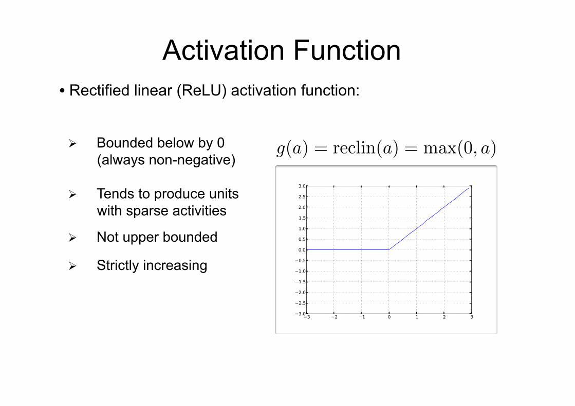
Activation Function • Rectified linear (ReLU) activation function:
Feedforward neural network
Hugo LarochelleD
´
epartement d’informatique
Universit
´
e de Sherbrooke
September 6, 2012
Abstract
Math for my slides “Feedforward neural network”.
• a(x) = b+
Pi wixi = b+w
>x
• h(x) = g(a(x)) = g(b+
Pi wixi)
• x
1
xd b w
1
wd
• w
• {
• g(a) = a
• g(a) = sigm(a) =
1
1+exp(�a)
• g(a) = tanh(a) =
exp(a)�exp(�a)exp(a)+exp(�a) =
exp(2a)�1
exp(2a)+1
• g(a) = max(0, a)
• g(a) = reclin(a) = max(0, a)
• g(·) b
• h(x) = g(a(x))
• a(x) = b
(1)
+W
(1)
x
⇣a(x)i = b
(1)
i
Pj W
(1)
i,j xj
⌘
• o(x) = g
(out)
(b
(2)
+w
(2)
>x)
1
Ø Bounded below by 0 (always non-negative)
Ø Tends to produce units with sparse activities
Ø Not upper bounded
Ø Strictly increasing
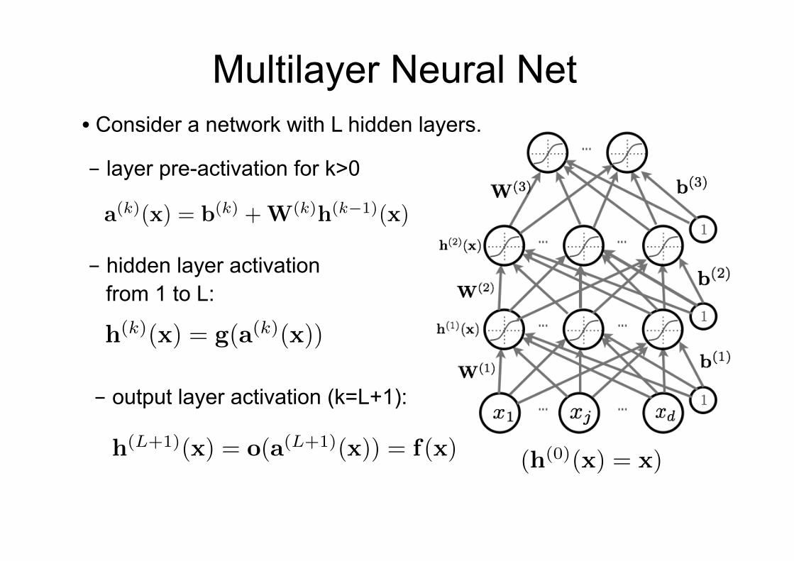
Multilayer Neural Net • Consider a network with L hidden layers.
- hidden layer activation from 1 to L:
- layer pre-activation for k>0
• p(y = c|x)
• o(a) = softmax(a) =
hexp(a1)Pc exp(ac)
. . .
exp(aC)Pc exp(ac)
i>
• f(x)
• h
(1)
(x) h
(2)
(x) W
(1)
W
(2)
W
(3)
b
(1)
b
(2)
b
(3)
• a
(k)(x) = b
(k)+W
(k)h
(k�1)
(x) (h
(0)
(x) = x)
• h
(k)(x) = g(a
(k)(x))
• h
(L+1)
(x) = o(a
(L+1)
(x)) = f(x)
2
• p(y = c|x)
• o(a) = softmax(a) =
hexp(a1)Pc exp(ac)
. . .
exp(aC)Pc exp(ac)
i>
• f(x)
• h
(1)
(x) h
(2)
(x) W
(1)
W
(2)
W
(3)
b
(1)
b
(2)
b
(3)
• a
(k)(x) = b
(k)+W
(k)h
(k�1)
x (h
(0)
= x)
• h
(k)(x) = g(a
(k)(x))
• h
(L+1)
(x) = o(a
(L+1)
(x)) = f(x)
2
• p(y = c|x)
• o(a) = softmax(a) =
hexp(a1)Pc exp(ac)
. . .
exp(aC)Pc exp(ac)
i>
• f(x)
• h
(1)
(x) h
(2)
(x) W
(1)
W
(2)
W
(3)
b
(1)
b
(2)
b
(3)
• a
(k)(x) = b
(k)+W
(k)h
(k�1)
x (h
(0)
= x)
• h
(k)(x) = g(a
(k)(x))
• h
(L+1)
(x) = o(a
(L+1)
(x)) = f(x)
2
- output layer activation (k=L+1):
• p(y = c|x)
• o(a) = softmax(a) =
hexp(a1)Pc exp(ac)
. . .
exp(aC)Pc exp(ac)
i>
• f(x)
• h
(1)
(x) h
(2)
(x) W
(1)
W
(2)
W
(3)
b
(1)
b
(2)
b
(3)
• a
(k)(x) = b
(k)+W
(k)h
(k�1)
x (h
(0)
(x) = x)
• h
(k)(x) = g(a
(k)(x))
• h
(L+1)
(x) = o(a
(L+1)
(x)) = f(x)
2

Deep Neural Networks
Today: a brief introduction to deep neural networks
Definitions
Power of deep neural networksNeural networks / distributed representations vs kernel / localrepresentationsUniversal function approximatorDeep neural networks vs shallow neural networks
How to train neural nets
Emma Brunskill (CS234 Reinforcement Learning. )Lecture 5: Value Function Approximation
46
Winter 2018 42 / 44
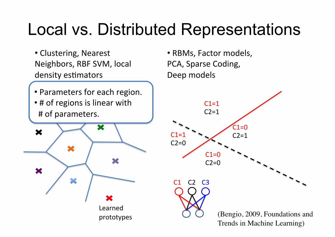
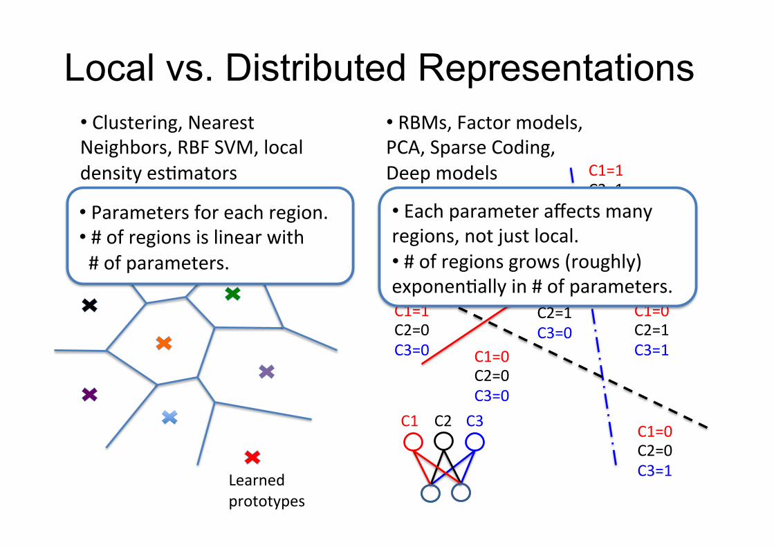
• Clustering,NearestNeighbors,RBFSVM,local
densityesFmators
Learned
prototypes
LocalregionsC1=1
C1=0
C2=1
C2=1C1=1C2=0
C1=0C2=0
• RBMs,Factormodels,PCA,SparseCoding,
Deepmodels
C2C1 C3
• Parametersforeachregion.• #ofregionsislinearwith#ofparameters.
(Bengio, 2009, Foundations and Trends in Machine Learning)
Local vs. Distributed Representations

• Clustering,NearestNeighbors,RBFSVM,local
densityesFmators
Learned
prototypes
Localregions
C3=0
C1=1
C1=0
C3=0C3=0
C2=1
C2=1C1=1C2=0
C1=0C2=0C3=0
C1=1C2=1C3=1
C1=0C2=1C3=1
C1=0C2=0C3=1
• RBMs,Factormodels,PCA,SparseCoding,
Deepmodels
• Parametersforeachregion.• #ofregionsislinearwith#ofparameters.
C2C1 C3
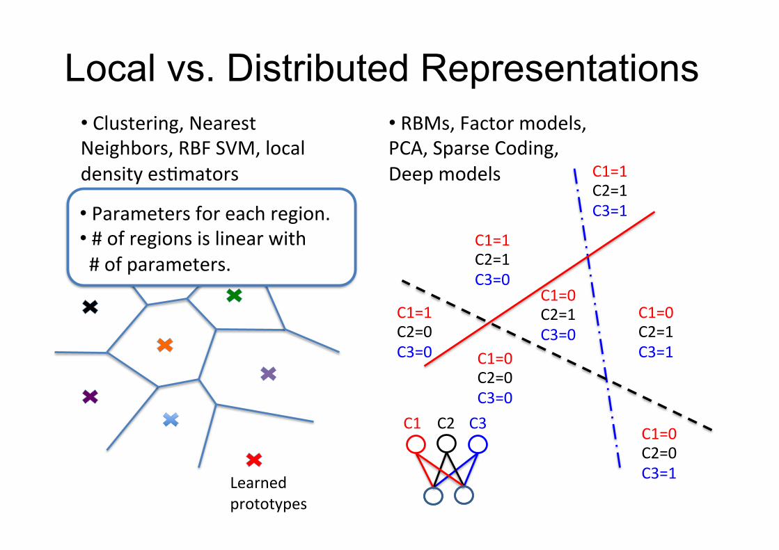
Local vs. Distributed Representations
• Clustering,NearestNeighbors,RBFSVM,local
densityesFmators
Learned
prototypes
Localregions
C3=0
C1=1
C1=0
C3=0C3=0
C2=1
C2=1C1=1C2=0
C1=0C2=0C3=0
C1=1C2=1C3=1
C1=0C2=1C3=1
C1=0C2=0C3=1
• RBMs,Factormodels,PCA,SparseCoding,
Deepmodels
• Parametersforeachregion.• #ofregionsislinearwith#ofparameters.
C2C1 C3
Local vs. Distributed Representations
• Clustering,NearestNeighbors,RBFSVM,local
densityesFmators
Learned
prototypes
Localregions
C3=0
C1=1
C1=0
C3=0C3=0
C2=1
C2=1C1=1C2=0
C1=0C2=0C3=0
C1=1C2=1C3=1
C1=0C2=1C3=1
C1=0C2=0C3=1
• RBMs,Factormodels,PCA,SparseCoding,
Deepmodels
• Parametersforeachregion.• #ofregionsislinearwith#ofparameters.
• Eachparameteraffectsmanyregions,notjustlocal.
• #ofregionsgrows(roughly)exponenFallyin#ofparameters.
C2C1 C3
Local vs. Distributed Representations
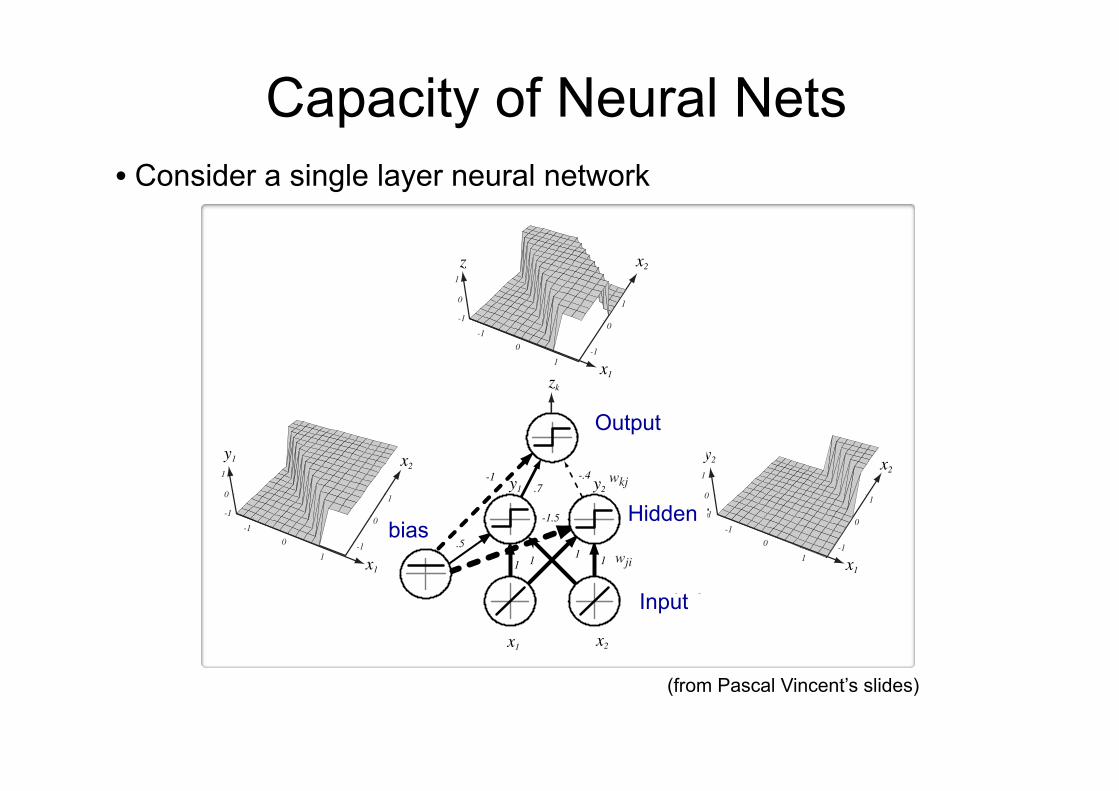
Capacity of Neural Nets • Consider a single layer neural network 2Reseaux de neurones
-1 1
-1
1
11
1 1
.5
-1.5
.7-.4-1
x1 x2
x1
x2
z=+1
z=-1
z=-1
0
1-1
0
1
-1
0
1
-1
0
1-1
0
1
-1
0
1
-1
0
1-1
0
1
-1
0
1
-1
R2
R2
R1
y1 y2
z
zk
wkj
wji
x1
x2
x1
x2
x1
x2
y1 y2
sortie k
entree i
cachee jbiais
Input
Hidden
Output
bias
(from Pascal Vincent’s slides)
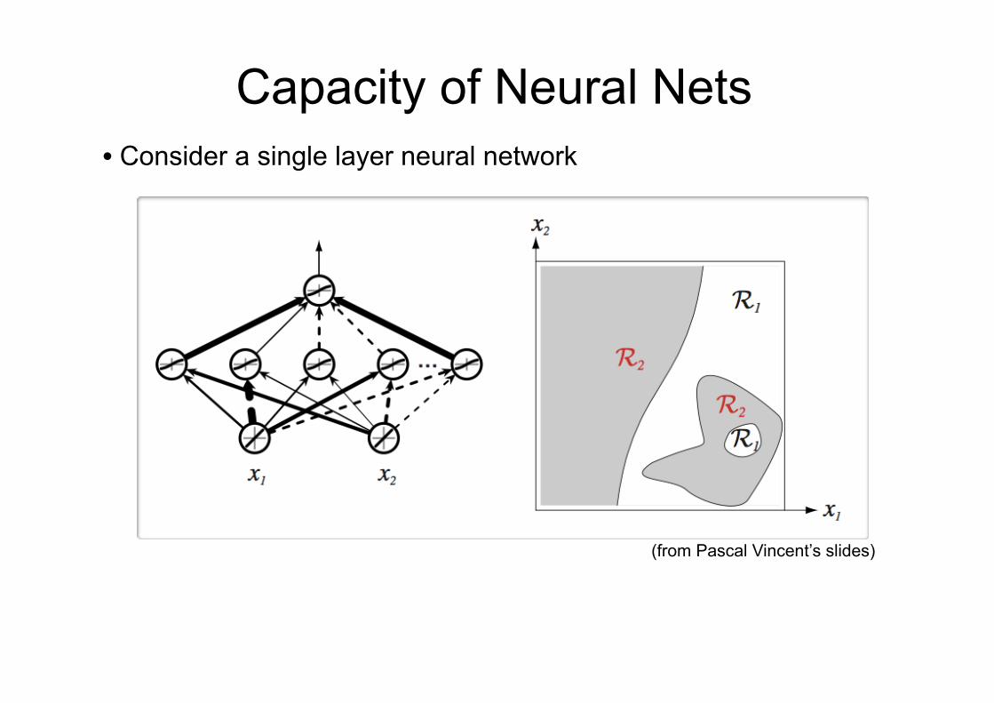
Capacity of Neural Nets • Consider a single layer neural network
(from Pascal Vincent’s slides)

Universal Approximation • Universal Approximation Theorem (Hornik, 1991):
- “a single hidden layer neural network with a linear output unit can approximate any continuous function arbitrarily well, given enough hidden units’’
• This applies for sigmoid, tanh and many other activation functions.
• However, this does not mean that there is learning algorithm that can find the necessary parameter values.

Deep Networks vs Shallow
1 hidden layer neural networks are already a universal functionapproximator
Implies the expressive power of deep networks are no larger thanshallow networks
There always exists a shallow network that can represent any functionrepresentable by a deep (multi-layer) neural network
But there can be cases where deep networks may be exponentiallymore compact than shallow networks in terms of number of nodesrequired to represent a function
This has substantial implications for memory, computation and datae�ciency
Empirically often deep networks outperform shallower alternatives
Emma Brunskill (CS234 Reinforcement Learning. )Lecture 5: Value Function Approximation
47
Winter 2018 43 / 44
Deep Neural Networks
Today: a brief introduction to deep neural networks
Definitions
Power of deep neural networksNeural networks / distributed representations vs kernel / localrepresentationsUniversal function approximatorDeep neural networks vs shallow neural networks
How to train neural nets
Emma Brunskill (CS234 Reinforcement Learning. )Lecture 5: Value Function Approximation
48
Winter 2018 44 / 44

Feedforward Neural Networks ‣ How neural networks predict f(x) given an input x:
- Forward propagation - Types of units - Capacity of neural networks
‣ How to train neural nets: - Loss function - Backpropagation with gradient descent
‣ More recent techniques: - Dropout - Batch normalization - Unsupervised Pre-training
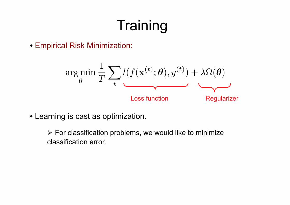
Training • Empirical Risk Minimization:
• bµ =
1T
Pt x
(t)
• b�2=
1T�1
Pt(x
(t) � bµ)2
• b⌃ =
1T�1
Pt(x
(t) � bµ)(x(t) � bµ)>
• E[
bµ] = µ E[b�2] = �2
E
hb⌃
i= ⌃
• bµ�µpb�2/T
• µ 2 bµ±�1.96p
b�2/T
•b✓ = argmax
✓p(x(1), . . . ,x(T )
)
•p(x(1), . . . ,x(T )
) =
Y
t
p(x(t))
• T�1T
b⌃ =
1T
Pt(x
(t) � bµ)(x(t) � bµ)>
Machine learning
• Supervised learning example: (x, y) x y
• Training set: Dtrain= {(x(t), y(t))}
• f(x;✓)
• Dvalid Dtest
•argmin
✓
1
T
X
t
l(f(x(t);✓), y(t)) + �⌦(✓)
5
Loss function Regularizer
• Learning is cast as optimization.
Ø For classification problems, we would like to minimize classification error.
Ø Loss function can sometimes be viewed as a surrogate for what we want to optimize (e.g. upper bound)

Stochastic Gradient Descend • Perform updates after seeing each example: - Initialize:
Feedforward neural network
Hugo LarochelleD
´
epartement d’informatique
Universit´e de Sherbrooke
September 13, 2012
Abstract
Math for my slides “Feedforward neural network”.
• f(x)
• ✓ ⌘ {W(1),b(1), . . . ,W(L+1),b(L+1)}
• l(f(x(t);✓), y(t))
• r✓l(f(x(t);✓), y(t))
• ⌦(✓)
• r✓⌦(✓)
• f(x)c = p(y = c|x)
• x
(t) y(t)
• l(f(x), y) = �P
c 1(y=c) log f(x)c = � log f(x)y =
•
@
f(x)c� log f(x)y =
�1(y=c)
f(x)y
rf(x) � log f(x)y =
�1
f(x)y[1(y=0), . . . , 1(y=C�1)]
>
=
�e(c)
f(x)y
1
- For t=1:T - for each training example
• bµ =
1T
Pt x
(t)
• b�2=
1T�1
Pt(x
(t) � bµ)2
• b⌃ =
1T�1
Pt(x
(t) � bµ)(x(t) � bµ)>
• E[
bµ] = µ E[b�2] = �2
E
hb⌃
i= ⌃
• bµ�µpb�2/T
• µ 2 bµ±�1.96p
b�2/T
•b✓ = argmax
✓p(x(1), . . . ,x(T )
)
•p(x(1), . . . ,x(T )
) =
Y
t
p(x(t))
• T�1T
b⌃ =
1T
Pt(x
(t) � bµ)(x(t) � bµ)>
Machine learning
• Supervised learning example: (x, y) x y
• Training set: Dtrain= {(x(t), y(t))}
• f(x;✓)
• Dvalid Dtest
•argmin
✓
1
T
X
t
l(f(x(t);✓), y(t)) + �⌦(✓)
• l(f(x(t);✓), y(t))
• ⌦(✓)
• � = � 1T
Ptr✓l(f(x
(t);✓), y(t))� �r✓⌦(✓)
• ✓ ✓ +�
• {x 2 Rd | rx
f(x) = 0}
• v
>r2x
f(x)v > 0 8v
• v
>r2x
f(x)v < 0 8v
• � = �r✓l(f(x(t);✓), y(t))� �r✓⌦(✓)
• (x
(t), y(t))
5
• bµ =
1T
Pt x
(t)
• b�2=
1T�1
Pt(x
(t) � bµ)2
• b⌃ =
1T�1
Pt(x
(t) � bµ)(x(t) � bµ)>
• E[
bµ] = µ E[b�2] = �2
E
hb⌃
i= ⌃
• bµ�µpb�2/T
• µ 2 bµ±�1.96p
b�2/T
•b✓ = argmax
✓p(x(1), . . . ,x(T )
)
•p(x(1), . . . ,x(T )
) =
Y
t
p(x(t))
• T�1T
b⌃ =
1T
Pt(x
(t) � bµ)(x(t) � bµ)>
Machine learning
• Supervised learning example: (x, y) x y
• Training set: Dtrain= {(x(t), y(t))}
• f(x;✓)
• Dvalid Dtest
•argmin
✓
1
T
X
t
l(f(x(t);✓), y(t)) + �⌦(✓)
• l(f(x(t);✓), y(t))
• ⌦(✓)
• � = � 1T
Ptr✓l(f(x
(t);✓), y(t))� �r✓⌦(✓)
• ✓ ✓ +�
• {x 2 Rd | rx
f(x) = 0}
• v
>r2x
f(x)v > 0 8v
• v
>r2x
f(x)v < 0 8v
• � = �r✓l(f(x(t);✓), y(t))� �r✓⌦(✓)
5
•argmin
✓
1
T
X
t
l(f(x(t);✓), y(t)) + �⌦(✓)
• l(f(x(t);✓), y(t))
• ⌦(✓)
• � = � 1T
Ptr✓l(f(x
(t);✓), y(t))� �r✓⌦(✓)
• ✓ ✓ + ↵ �
• {x 2 Rd | rx
f(x) = 0}
• v
>r2x
f(x)v > 0 8v
• v
>r2x
f(x)v < 0 8v
• � = �r✓l(f(x(t);✓), y(t))� �r✓⌦(✓)
• (x
(t), y(t))
• f⇤ f
6
Training epoch =
Iteration of all examples
• To train a neural net, we need:
Ø Loss function: Ø A procedure to compute gradients: Ø Regularizer and its gradient: ,
Feedforward neural network
Hugo LarochelleD
´
epartement d’informatique
Universit´e de Sherbrooke
September 13, 2012
Abstract
Math for my slides “Feedforward neural network”.
• f(x)
• l(f(x(t);✓), y(t))
• r✓l(f(x(t);✓), y(t))
• ⌦(✓)
• r✓⌦(✓)
• f(x)c = p(y = c|x)
• x
(t) y(t)
• l(f(x), y) = �P
c 1(y=c) log f(x)c = � log f(x)y =
•
@
f(x)c� log f(x)y =
�1(y=c)
f(x)y
rf(x) � log f(x)y =
�1
f(x)y[1(y=0), . . . , 1(y=C�1)]
>
=
�e(c)
f(x)y
1

Computational Flow Graph • Forward propagation can be represented as an acyclic flow graph
• Forward propagation can be implemented in a modular way:
Ø Each box can be an object with an fprop method, that computes the value of the box given its children
Ø Calling the fprop method of each box in the right order yields forward propagation

• Each object also has a bprop method
• By calling bprop in the reverse order, we obtain backpropagation
- it computes the gradient of the loss with respect to each child box.
Computational Flow Graph
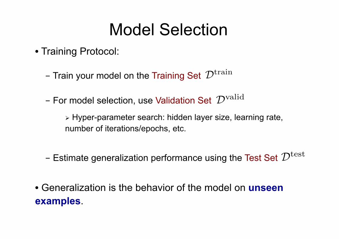
Model Selection • Training Protocol:
- Train your model on the Training Set
• bµ =
1T
Pt x
(t)
• b�2=
1T�1
Pt(x
(t) � bµ)2
• b⌃ =
1T�1
Pt(x
(t) � bµ)(x(t) � bµ)>
• E[
bµ] = µ E[b�2] = �2
E
hb⌃
i= ⌃
• bµ�µpb�2/T
• µ 2 bµ±�1.96p
b�2/T
•b✓ = argmax
✓p(x(1), . . . ,x(T )
)
•p(x(1), . . . ,x(T )
) =
Y
t
p(x(t))
• T�1T
b⌃ =
1T
Pt(x
(t) � bµ)(x(t) � bµ)>
Machine learning
• Supervised learning example: (x, y) x y
• Training set: Dtrain= {(x(t), y(t))}
• f(x;✓)
5
- For model selection, use Validation Set
• bµ =
1T
Pt x
(t)
• b�2=
1T�1
Pt(x
(t) � bµ)2
• b⌃ =
1T�1
Pt(x
(t) � bµ)(x(t) � bµ)>
• E[
bµ] = µ E[b�2] = �2
E
hb⌃
i= ⌃
• bµ�µpb�2/T
• µ 2 bµ±�1.96p
b�2/T
•b✓ = argmax
✓p(x(1), . . . ,x(T )
)
•p(x(1), . . . ,x(T )
) =
Y
t
p(x(t))
• T�1T
b⌃ =
1T
Pt(x
(t) � bµ)(x(t) � bµ)>
Machine learning
• Supervised learning example: (x, y) x y
• Training set: Dtrain= {(x(t), y(t))}
• f(x;✓)
• Dvalid Dtest
5
Ø Hyper-parameter search: hidden layer size, learning rate, number of iterations/epochs, etc.
- Estimate generalization performance using the Test Set
• bµ =
1T
Pt x
(t)
• b�2=
1T�1
Pt(x
(t) � bµ)2
• b⌃ =
1T�1
Pt(x
(t) � bµ)(x(t) � bµ)>
• E[
bµ] = µ E[b�2] = �2
E
hb⌃
i= ⌃
• bµ�µpb�2/T
• µ 2 bµ±�1.96p
b�2/T
•b✓ = argmax
✓p(x(1), . . . ,x(T )
)
•p(x(1), . . . ,x(T )
) =
Y
t
p(x(t))
• T�1T
b⌃ =
1T
Pt(x
(t) � bµ)(x(t) � bµ)>
Machine learning
• Supervised learning example: (x, y) x y
• Training set: Dtrain= {(x(t), y(t))}
• f(x;✓)
• Dvalid Dtest
5
• Generalization is the behavior of the model on unseen examples.
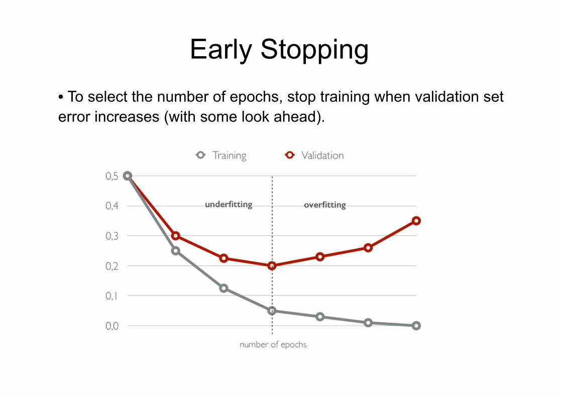
Early Stopping • To select the number of epochs, stop training when validation set error increases (with some look ahead).
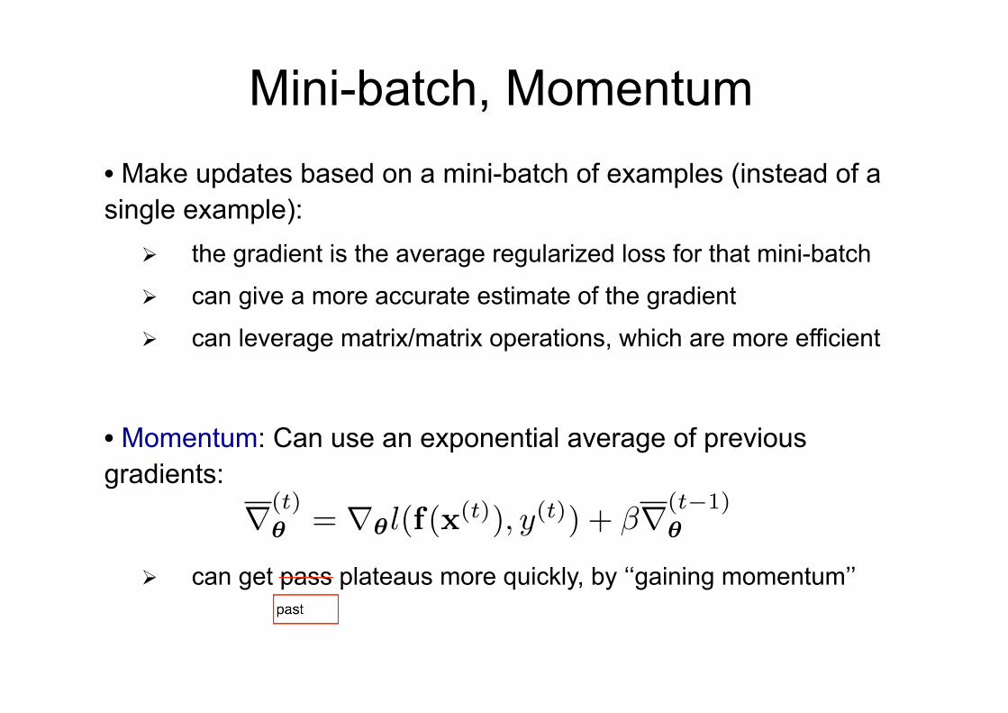
Mini-batch, Momentum • Make updates based on a mini-batch of examples (instead of a single example):
Ø the gradient is the average regularized loss for that mini-batch
Ø can give a more accurate estimate of the gradient
Ø can leverage matrix/matrix operations, which are more efficient
• Momentum: Can use an exponential average of previous gradients:
• g0(a) = g(a)(1� g(a))
• g0(a) = 1� g(a)2
• ⌦(✓) =P
k
Pi
Pj
⇣W
(k)i,j
⌘2=
Pk ||W(k)||2F
• rW
(k)⌦(✓) = 2W
(k)
• ⌦(✓) =P
k
Pi
Pj |W
(k)i,j |
• rW
(k)⌦(✓) = sign(W
(k))
• sign(W
(k))i,j = 1
W
(k)i,j >0
� 1
W
(k)i,j <0
• W
(k)i,j U [�b, b] b =
p6p
Hk+Hk�1Hk h
(k)(x)
• a
(3)(x) = b
(3)+W
(3)h
(2)
• a
(2)(x) = b
(2)+W
(2)h
(1)
• a
(1)(x) = b
(1)+W
(1)x
• h
(3)(x) = o(a
(3)(x))
• h
(2)(x) = g(a
(2)(x))
• h
(1)(x) = g(a
(1)(x))
• b
(3)b
(2)b
(1)
• W
(3)W
(2)W
(1)x f(x)
• @f(x)@x ⇡ f(x+✏)�f(x�✏)
2✏
• f(x) x ✏
• f(x+ ✏) f(x� ✏)
•P1
t=1 ↵t = 1
•P1
t=1 ↵2t < 1 ↵t
• ↵t =↵
1+�t
• ↵t =↵t�
0.5 < � 1 �
• r(t)✓ = r✓l(f(x
(t)), y(t)) + �r(t�1)
✓
4
Ø can get pass plateaus more quickly, by ‘‘gaining momentum’’
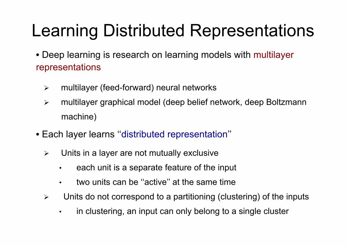
Learning Distributed Representations • Deep learning is research on learning models with multilayer representations
Ø multilayer (feed-forward) neural networks
Ø multilayer graphical model (deep belief network, deep Boltzmann
machine)
• Each layer learns ‘‘distributed representation’’
Ø Units in a layer are not mutually exclusive
• each unit is a separate feature of the input
• two units can be ‘‘active’’ at the same time
Ø Units do not correspond to a partitioning (clustering) of the inputs
• in clustering, an input can only belong to a single cluster
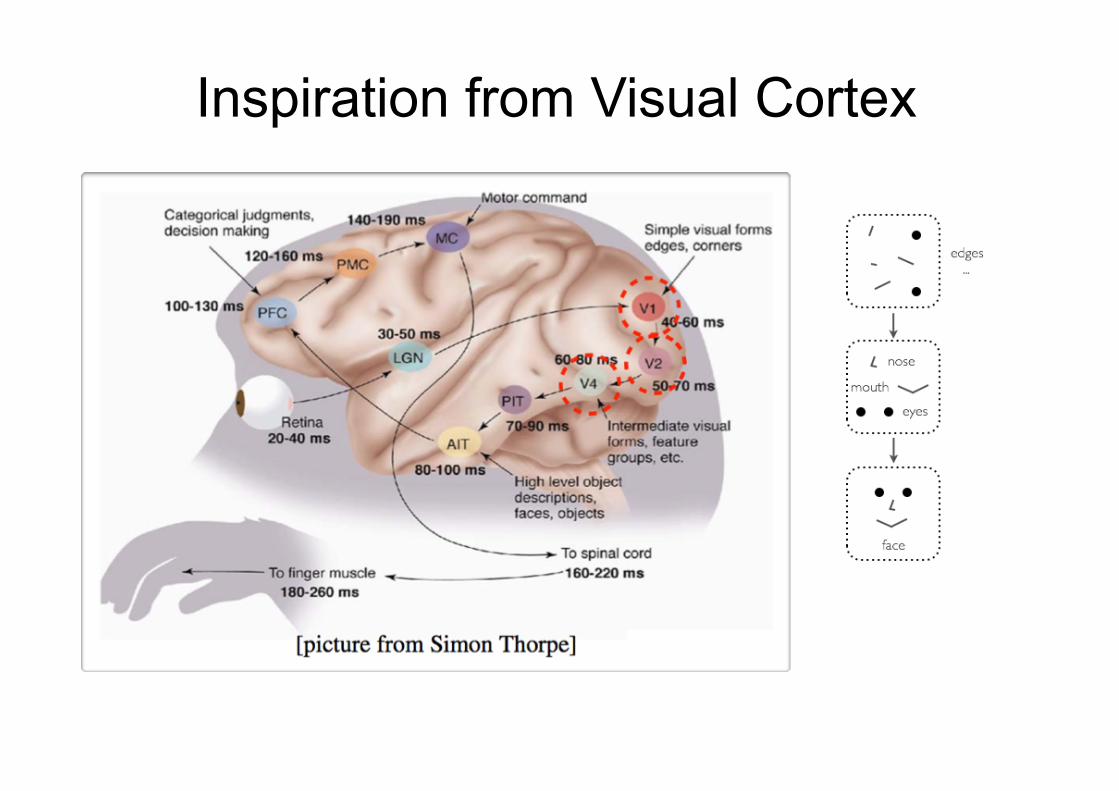
Inspiration from Visual Cortex

Feedforward Neural Networks ‣ How neural networks predict f(x) given an input x:
- Forward propagation - Types of units - Capacity of neural networks
‣ How to train neural nets: - Loss function - Backpropagation with gradient descent
‣ More recent techniques: - Dropout - Batch normalization - Unsupervised Pre-training

Why Training is Hard • First hypothesis: Hard optimization problem (underfitting)
Ø vanishing gradient problem
Ø saturated units block gradient
propagation
• This is a well known problem in recurrent neural networks
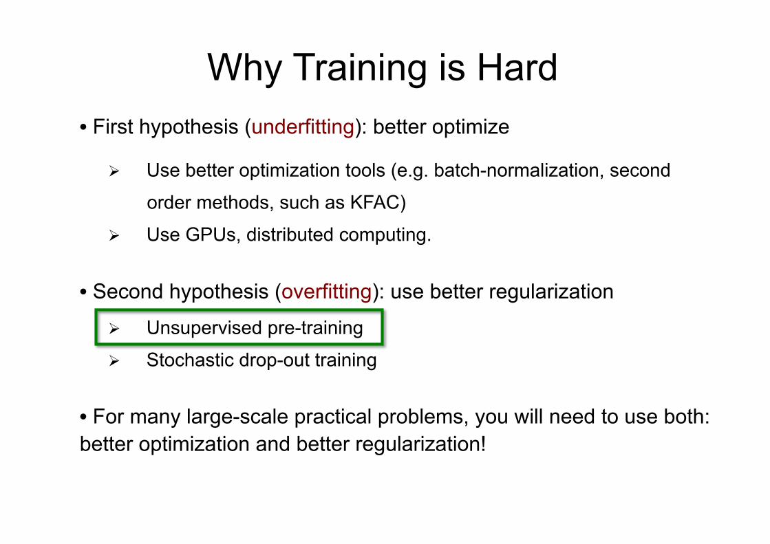
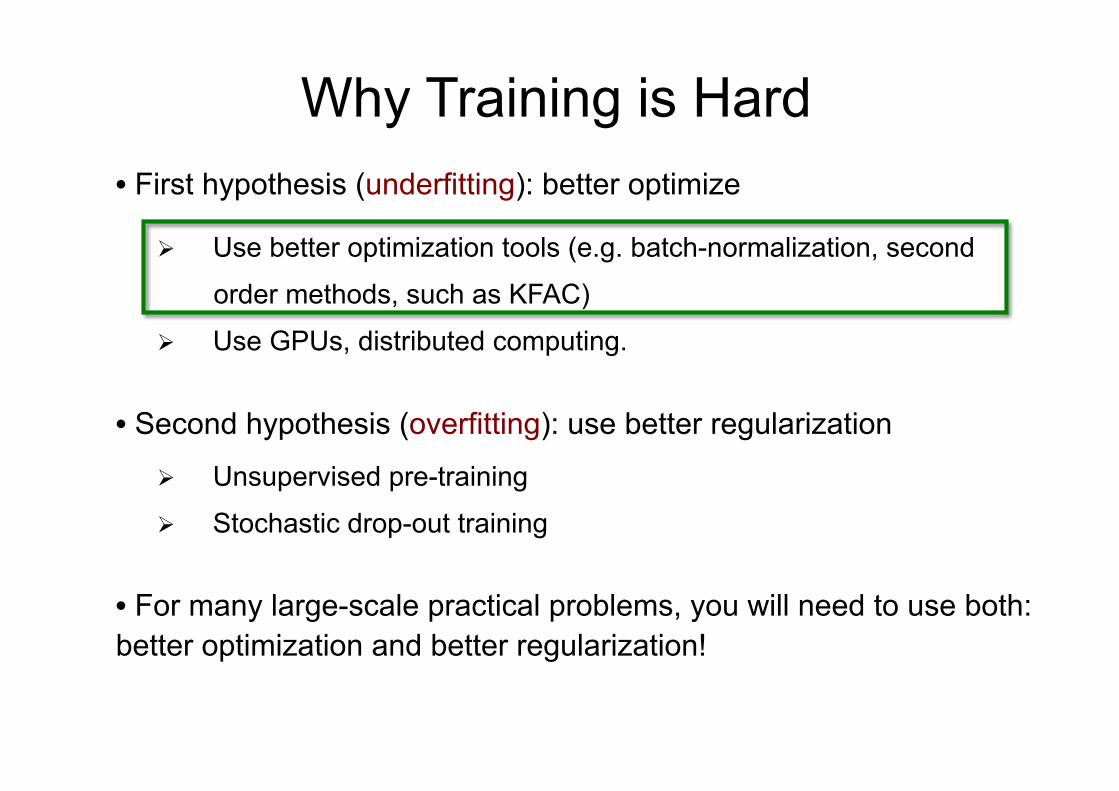
Why Training is Hard • First hypothesis (underfitting): better optimize
Ø Use better optimization tools (e.g. batch-normalization, second
order methods, such as KFAC)
Ø Use GPUs, distributed computing.
• Second hypothesis (overfitting): use better regularization
Ø Unsupervised pre-training
Ø Stochastic drop-out training
• For many large-scale practical problems, you will need to use both: better optimization and better regularization!

Unsupervised Pre-training • Initialize hidden layers using unsupervised learning
Ø Force network to represent latent structure of input distribution
Ø Encourage hidden layers to encode that structure
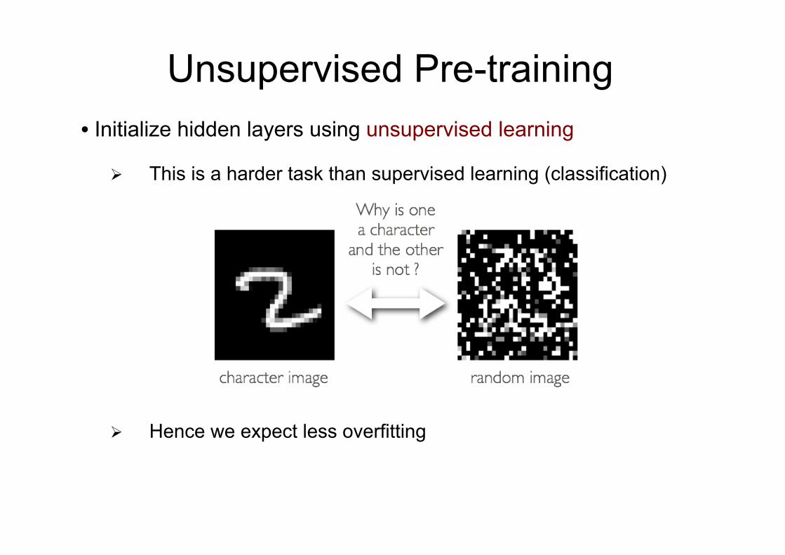
Unsupervised Pre-training • Initialize hidden layers using unsupervised learning
Ø This is a harder task than supervised learning (classification)
Ø Hence we expect less overfitting

Autoencoders: Preview • Feed-forward neural network trained to reproduce its input at the output layer
Autoencoders
Hugo LarochelleDepartement d’informatique
Universite de [email protected]
October 16, 2012
Abstract
Math for my slides “Autoencoders”.
•
h(x) = g(a(x))
= sigm(b+Wx)
•
bx = o(
ba(x))
= sigm(c+W
⇤h(x))
• f(x) ⌘ bx l(f(x)) =
Pk(bxk � xk)
2l(f(x)) = �
Pk (xk log(bxk) + (1� xk) log(1� bxk))
1
Decoder
Autoencoders
Hugo LarochelleDepartement d’informatique
Universite de [email protected]
October 16, 2012
Abstract
Math for my slides “Autoencoders”.
•
h(x) = g(a(x))
= sigm(b+Wx)
•
bx = o(
ba(x))
= sigm(c+W
⇤h(x))
• f(x) ⌘ bx l(f(x)) =
Pk(bxk � xk)
2l(f(x)) = �
Pk (xk log(bxk) + (1� xk) log(1� bxk))
1
Encoder
For binary units

Autoencoders: Preview • Loss function for binary inputs
Autoencoders
Hugo LarochelleDepartement d’informatique
Universite de [email protected]
October 16, 2012
Abstract
Math for my slides “Autoencoders”.
•
h(x) = g(b+Wx)
= sigm(b+Wx)
•
bx = o(c+W
⇤h(x))
= sigm(c+W
⇤h(x))
• f(x) ⌘ bx l(f(x)) =
Pk(bxk � xk)
2l(f(x)) = �
Pk (xk log(bxk) + (1� xk) log(1� bxk))
1
Ø Cross-entropy error function
Autoencoders
Hugo LarochelleDepartement d’informatique
Universite de [email protected]
October 16, 2012
Abstract
Math for my slides “Autoencoders”.
•
h(x) = g(a(x))
= sigm(b+Wx)
•
bx = o(
ba(x))
= sigm(c+W
⇤h(x))
• f(x) ⌘ bx l(f(x)) =
12
Pk(bxk � xk)
2l(f(x)) = �
Pk (xk log(bxk) + (1� xk) log(1� bxk))
• rba(x(t))l(f(x
(t))) =
bx
(t) � x
(t)
a(x
(t)) (= b+Wx
(t)
h(x
(t)) (= sigm(a(x
(t)))
ba(x
(t)) (= c+W
>h(x
(t))
bx
(t) (= sigm(
ba(x
(t)))
rba(x(t))l(f(x
(t))) (=
bx
(t) � x
(t)
rc
l(f(x
(t))) (= rb
a(x(t))l(f(x(t)))
rh(x(t))l(f(x
(t))) (= W
⇣rb
a(x(t))l(f(x(t)))
⌘
ra(x(t))l(f(x
(t))) (=
⇣r
h(x(t))l(f(x(t)))
⌘� [. . . , h(x
(t))j(1� h(x
(t))j), . . . ]
rb
l(f(x
(t))) (= r
a(x(t))l(f(x(t)))
rW
l(f(x
(t))) (=
⇣r
a(x(t))l(f(x(t)))
⌘x
(t)>+ h(x
(t))
⇣rb
a(x(t))l(f(x(t)))
⌘>
• W
⇤= W
>
1
• Loss function for real-valued inputs
Ø sum of squared differences
Ø we use a linear activation function at the output
Autoencoders
Hugo LarochelleDepartement d’informatique
Universite de [email protected]
October 16, 2012
Abstract
Math for my slides “Autoencoders”.
•
h(x) = g(b+Wx)
= sigm(b+Wx)
•
bx = o(c+W
⇤h(x))
= sigm(c+W
⇤h(x))
• f(x) ⌘ bx l(f(x)) =
Pk(bxk � xk)2
1
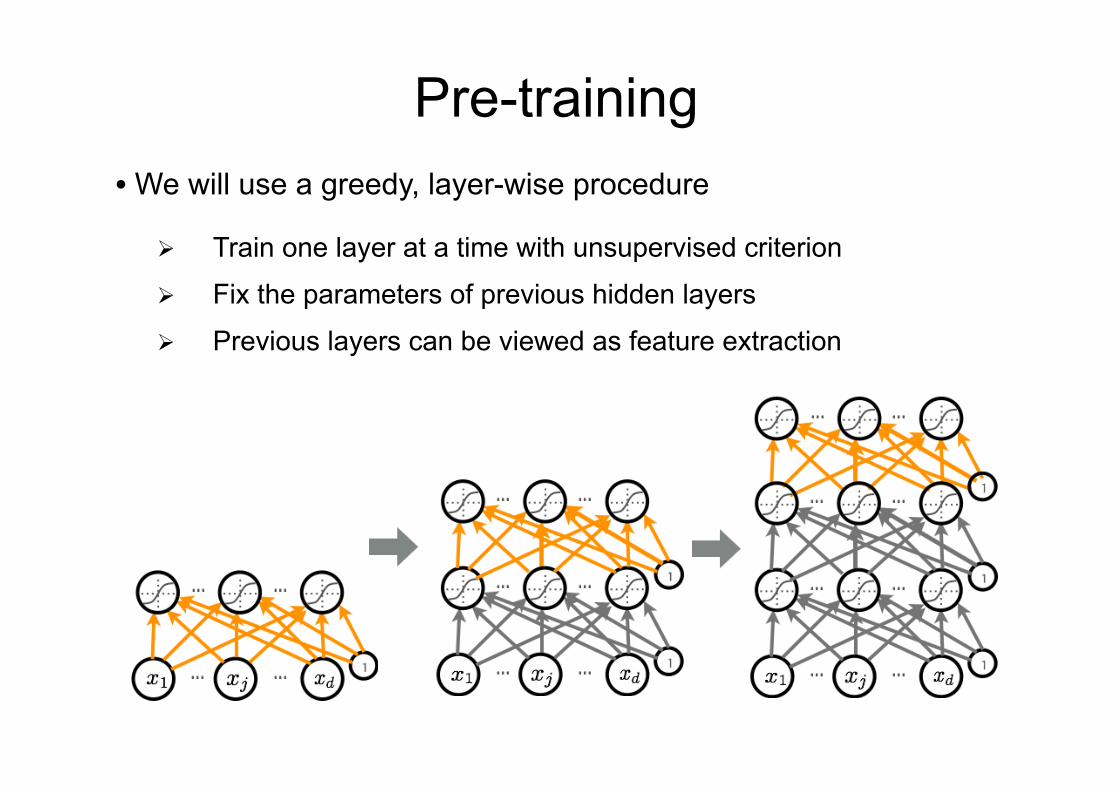
Pre-training • We will use a greedy, layer-wise procedure
Ø Train one layer at a time with unsupervised criterion
Ø Fix the parameters of previous hidden layers
Ø Previous layers can be viewed as feature extraction
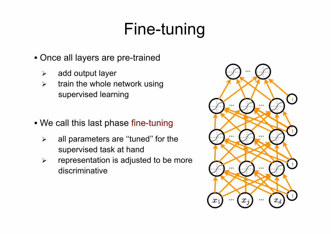
Fine-tuning • Once all layers are pre-trained
Ø add output layer Ø train the whole network using
supervised learning
• We call this last phase fine-tuning
Ø all parameters are ‘‘tuned’’ for the supervised task at hand
Ø representation is adjusted to be more discriminative
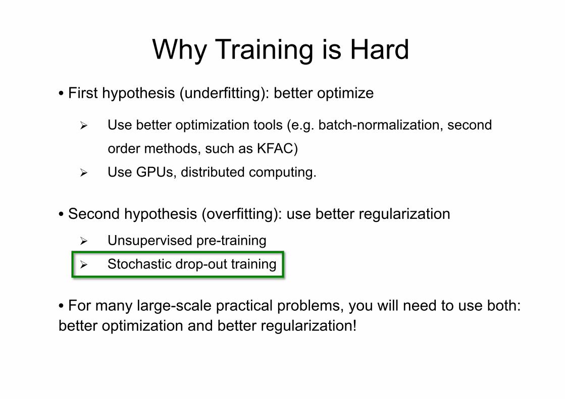
Why Training is Hard • First hypothesis (underfitting): better optimize
Ø Use better optimization tools (e.g. batch-normalization, second
order methods, such as KFAC)
Ø Use GPUs, distributed computing.
• Second hypothesis (overfitting): use better regularization
Ø Unsupervised pre-training
Ø Stochastic drop-out training
• For many large-scale practical problems, you will need to use both: better optimization and better regularization!

Dropout • Key idea: Cripple neural network by removing hidden units stochastically
Ø each hidden unit is set to 0 with probability 0.5
Ø hidden units cannot co-adapt to other units
Ø hidden units must be more generally useful
• Could use a different dropout probability, but 0.5 usually works well

Dropout • Use random binary masks m(k)
Ø layer pre-activation for k>0
• p(y = c|x)
• o(a) = softmax(a) =
hexp(a1)Pc exp(ac)
. . .
exp(aC)Pc exp(ac)
i>
• f(x)
• h
(1)
(x) h
(2)
(x) W
(1)
W
(2)
W
(3)
b
(1)
b
(2)
b
(3)
• a
(k)(x) = b
(k)+W
(k)h
(k�1)
(x) (h
(0)
(x) = x)
• h
(k)(x) = g(a
(k)(x))
• h
(L+1)
(x) = o(a
(L+1)
(x)) = f(x)
2
Ø hidden layer activation (k=1 to L):
• p(y = c|x)
• o(a) = softmax(a) =
hexp(a1)Pc exp(ac)
. . .
exp(aC)Pc exp(ac)
i>
• f(x)
• h
(1)
(x) h
(2)
(x) W
(1)
W
(2)
W
(3)
b
(1)
b
(2)
b
(3)
• a
(k)(x) = b
(k)+W
(k)h
(k�1)
x (h
(0)
= x)
• h
(k)(x) = g(a
(k)(x))
• h
(L+1)
(x) = o(a
(L+1)
(x)) = f(x)
2
Ø Output activation (k=L+1)
• p(y = c|x)
• o(a) = softmax(a) =
hexp(a1)Pc exp(ac)
. . .
exp(aC)Pc exp(ac)
i>
• f(x)
• h
(1)
(x) h
(2)
(x) W
(1)
W
(2)
W
(3)
b
(1)
b
(2)
b
(3)
• a
(k)(x) = b
(k)+W
(k)h
(k�1)
x (h
(0)
= x)
• h
(k)(x) = g(a
(k)(x))
• h
(L+1)
(x) = o(a
(L+1)
(x)) = f(x)
2
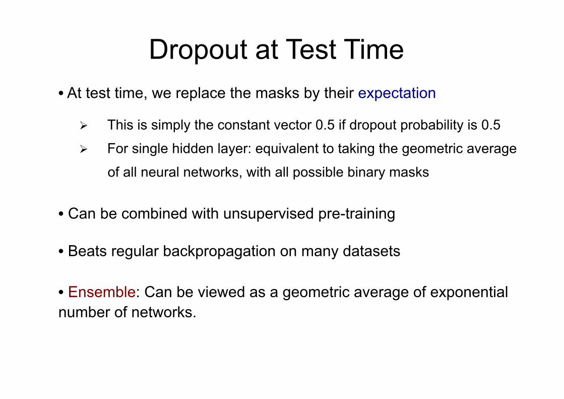
Dropout at Test Time • At test time, we replace the masks by their expectation
Ø This is simply the constant vector 0.5 if dropout probability is 0.5
Ø For single hidden layer: equivalent to taking the geometric average
of all neural networks, with all possible binary masks
• Can be combined with unsupervised pre-training
• Beats regular backpropagation on many datasets
• Ensemble: Can be viewed as a geometric average of exponential number of networks.
Why Training is Hard • First hypothesis (underfitting): better optimize
Ø Use better optimization tools (e.g. batch-normalization, second
order methods, such as KFAC)
Ø Use GPUs, distributed computing.
• Second hypothesis (overfitting): use better regularization
Ø Unsupervised pre-training
Ø Stochastic drop-out training
• For many large-scale practical problems, you will need to use both: better optimization and better regularization!
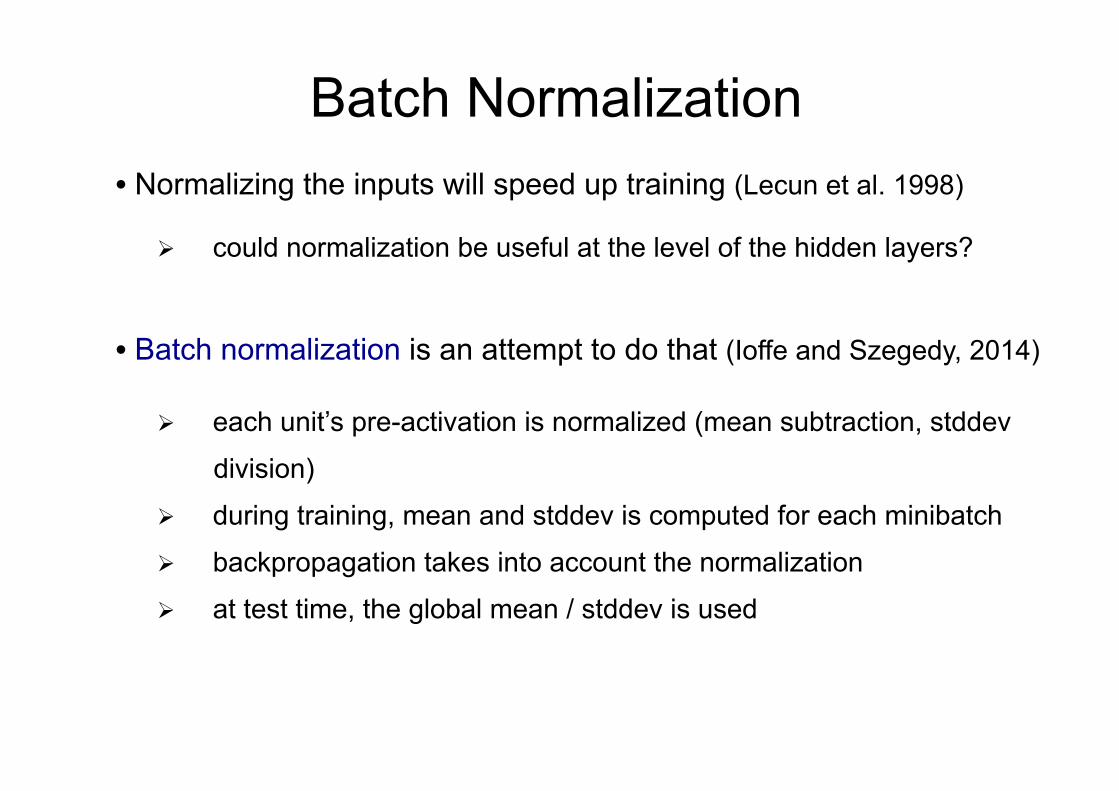
Batch Normalization • Normalizing the inputs will speed up training (Lecun et al. 1998)
Ø could normalization be useful at the level of the hidden layers?
• Batch normalization is an attempt to do that (Ioffe and Szegedy, 2014)
Ø each unit’s pre-activation is normalized (mean subtraction, stddev
division)
Ø during training, mean and stddev is computed for each minibatch
Ø backpropagation takes into account the normalization
Ø at test time, the global mean / stddev is used

Batch Normalization
Learned linear transformation to adapt to non-linear activation function (! and β are trained) and β are trained)
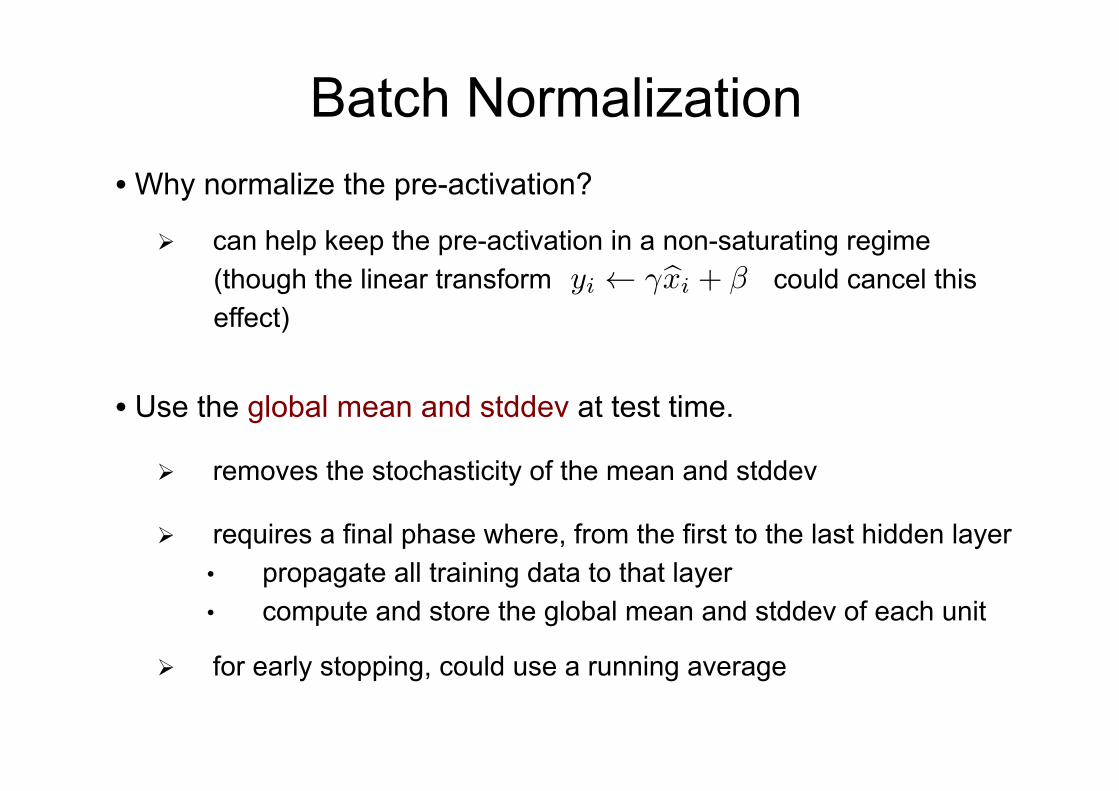
• Why normalize the pre-activation?
Ø can help keep the pre-activation in a non-saturating regime (though the linear transform could cancel this effect)
vector, and X be the set of these inputs over the trainingdata set. The normalization can then be written as a trans-formation
!x = Norm(x,X )
which depends not only on the given training example xbut on all examples X – each of which depends on Θ ifx is generated by another layer. For backpropagation, wewould need to compute the Jacobians
∂Norm(x,X )
∂xand
∂Norm(x,X )
∂X;
ignoring the latter term would lead to the explosion de-scribed above. Within this framework, whitening the layerinputs is expensive, as it requires computing the covari-ance matrix Cov[x] = Ex∈X [xxT ] − E[x]E[x]T and itsinverse square root, to produce the whitened activationsCov[x]−1/2(x − E[x]), as well as the derivatives of thesetransforms for backpropagation. This motivates us to seekan alternative that performs input normalization in a waythat is differentiable and does not require the analysis ofthe entire training set after every parameter update.Some of the previous approaches (e.g.
(Lyu & Simoncelli, 2008)) use statistics computedover a single training example, or, in the case of imagenetworks, over different feature maps at a given location.However, this changes the representation ability of anetwork by discarding the absolute scale of activations.We want to a preserve the information in the network, bynormalizing the activations in a training example relativeto the statistics of the entire training data.
3 Normalization via Mini-BatchStatistics
Since the full whitening of each layer’s inputs is costlyand not everywhere differentiable, we make two neces-sary simplifications. The first is that instead of whiteningthe features in layer inputs and outputs jointly, we willnormalize each scalar feature independently, by making ithave the mean of zero and the variance of 1. For a layerwith d-dimensional input x = (x(1) . . . x(d)), we will nor-malize each dimension
!x(k) =x(k) − E[x(k)]"
Var[x(k)]
where the expectation and variance are computed over thetraining data set. As shown in (LeCun et al., 1998b), suchnormalization speeds up convergence, even when the fea-tures are not decorrelated.Note that simply normalizing each input of a layer may
change what the layer can represent. For instance, nor-malizing the inputs of a sigmoid would constrain them tothe linear regime of the nonlinearity. To address this, wemake sure that the transformation inserted in the networkcan represent the identity transform. To accomplish this,
we introduce, for each activation x(k), a pair of parametersγ(k),β(k), which scale and shift the normalized value:
y(k) = γ(k)!x(k) + β(k).
These parameters are learned along with the originalmodel parameters, and restore the representation powerof the network. Indeed, by setting γ(k) =
"Var[x(k)] and
β(k) = E[x(k)], we could recover the original activations,if that were the optimal thing to do.In the batch setting where each training step is based on
the entire training set, we would use the whole set to nor-malize activations. However, this is impractical when us-ing stochastic optimization. Therefore, we make the sec-ond simplification: since we use mini-batches in stochas-tic gradient training, each mini-batch produces estimatesof the mean and variance of each activation. This way, thestatistics used for normalization can fully participate inthe gradient backpropagation. Note that the use of mini-batches is enabled by computation of per-dimension vari-ances rather than joint covariances; in the joint case, reg-ularization would be required since the mini-batch size islikely to be smaller than the number of activations beingwhitened, resulting in singular covariance matrices.Consider a mini-batch B of size m. Since the normal-
ization is applied to each activation independently, let usfocus on a particular activation x(k) and omit k for clarity.We havem values of this activation in the mini-batch,
B = {x1...m}.
Let the normalized values be !x1...m, and their linear trans-formations be y1...m. We refer to the transform
BNγ,β : x1...m → y1...m
as the Batch Normalizing Transform. We present the BNTransform in Algorithm 1. In the algorithm, ϵ is a constantadded to the mini-batch variance for numerical stability.
Input: Values of x over a mini-batch: B = {x1...m};Parameters to be learned: γ, β
Output: {yi = BNγ,β(xi)}
µB ←1
m
m#
i=1
xi // mini-batch mean
σ2B ←
1
m
m#
i=1
(xi − µB)2 // mini-batch variance
!xi ←xi − µB"σ2B+ ϵ
// normalize
yi ← γ!xi + β ≡ BNγ,β(xi) // scale and shift
Algorithm 1: Batch Normalizing Transform, applied toactivation x over a mini-batch.
The BN transform can be added to a network to manip-ulate any activation. In the notation y = BNγ,β(x), we
3
Batch Normalization
• Use the global mean and stddev at test time.
Ø removes the stochasticity of the mean and stddev
Ø requires a final phase where, from the first to the last hidden layer • propagate all training data to that layer • compute and store the global mean and stddev of each unit
Ø for early stopping, could use a running average
Recommended