Lecture 22Relativistic Quantum Mechanics
Background
Why study relativistic quantum mechanics?
1 Many experimental phenomena cannot be understood within purelynon-relativistic domain.
e.g. quantum mechanical spin, emergence of new sub-atomicparticles, etc.
2 New phenomena appear at relativistic velocities.
e.g. particle production, antiparticles, etc.
3 Aesthetically and intellectually it would be profoundly unsatisfactoryif relativity and quantum mechanics could not be united.
Background
When is a particle relativistic?
1 When velocity approaches speed of light c or, more intrinsically,when energy is large compared to rest mass energy, mc2.
e.g. protons at CERN are accelerated to energies of ca. 300GeV(1GeV= 109eV) much larger than rest mass energy, 0.94 GeV.
2 Photons have zero rest mass and always travel at the speed of light– they are never non-relativistic!

Background
What new phenomena occur?
1 Particle production
e.g. electron-positron pairs by energetic !-rays in matter.
2 Vacuum instability: If binding energy of electron
Ebind =Z 2e4m
2!2> 2mc2
a nucleus with initially no electrons is instantly screened by creationof electron/positron pairs from vacuum
3 Spin: emerges naturally from relativistic formulation

Background
When does relativity intrude on QM?
1 When Ekin ! mc2, i.e. p ! mc
2 From uncertainty relation, !x!p > h, this translates to a length
!x >h
mc= "c
the Compton wavelength.
3 for massless particles, "c =", i.e. relativity always important for,e.g., photons.

Relativistic quantum mechanics: outline
1 Special relativity (revision and notation)
2 Klein-Gordon equation
3 Dirac equation
4 Quantum mechanical spin
5 Solutions of the Dirac equation
6 Relativistic quantum field theories
7 Recovery of non-relativistic limit

Special relativity (revision and notation)
Space-time is specified by a 4-vector
A contravariant 4-vector
x = (xµ) # (x0, x1, x2, x3) # (ct, x)
transformed into covariant 4-vector xµ = gµ!x! by Minkowskiimetric
(gµ!) = (gµ!) =
!
""#
1$1
$1$1
$
%%& , gµ!g!" = gµ" # #µ
",
Scalar product: x · y = xµyµ = xµy!gµ! = xµyµ

Special relativity (revision and notation)
Lorentz group: consists of linear transformations, ", preservingx · y , i.e. for xµ %& x !µ = "µ
!x! = x · y
x ! · y ! = gµ!x !µy !
!= gµ!"µ
#"!$' () *
= g#$
x#y$ = g#$x#y$
e.g. Lorentz transformation along x1
"µ! =
!
""#
! $!v/c$!v/c !
1 00 1
$
%%& , ! =1
(1$ v2/c2)1/2

Special relativity (revision and notation)
4-vectors classified as time-like or space-like
x2 = (ct)2 $ x2
1 forward time-like: x2 > 0, x0 > 0
2 backward time-like: x2 > 0, x0 < 0
3 space-like: x2 < 0

Special relativity (revision and notation)
Lorentz group splits up into four components:
1 Every LT maps time-like vectors (x2 > 0) into time-like vectors
2 Orthochronous transformations "00 > 0, preserve
forward/backward sign
3 Proper: det " = 1 (as opposed to $1)
4 Group of proper orthochronous transformation: L"+ – subgroup
of Lorentz group – excludes time-reversal and parity
T =
!
""#
$11
11
$
%%& , P =
!
""#
1$1
$1$1
$
%%&
5 Remaining components of group generated by
L#$ = TL"
+, L"$ = PL"
+, L#+ = TPL"
+.
Special relativity (revision and notation)
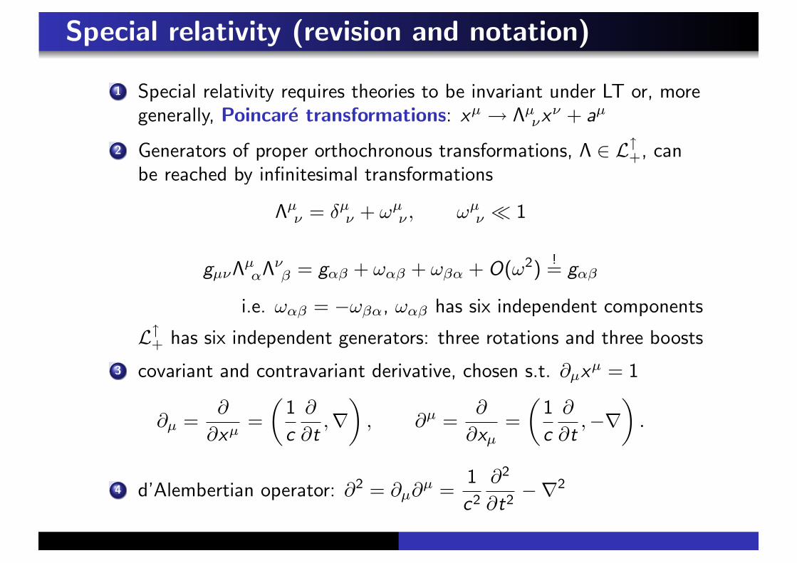
1 Special relativity requires theories to be invariant under LT or, moregenerally, Poincare transformations: xµ & "µ
!x! + aµ
2 Generators of proper orthochronous transformations, " ' L"+, can
be reached by infinitesimal transformations
"µ! = #µ
! + $µ! , $µ
! ( 1
gµ!"µ#"!
$ = g#$ + $#$ + $$# + O($2)!= g#$
i.e. $#$ = $$$#, $#$ has six independent components
L"+ has six independent generators: three rotations and three boosts
3 covariant and contravariant derivative, chosen s.t. %µxµ = 1
%µ =%
%xµ=
+1
c
%
%t,)
,, %µ =
%
%xµ=
+1
c
%
%t,$)
,.
4 d’Alembertian operator: %2 = %µ%µ =1
c2
%2
%t2$)2

Relativistic quantum mechanics: outline
1 Special relativity (revision and notation)
2 Klein-Gordon equation
3 Dirac equation
4 Quantum mechanical spin
5 Solutions of the Dirac equation
6 Relativistic quantum field theories
7 Recovery of non-relativistic limit

Klein-Gordon equation

Klein-Gordon equation
How to make wave equation relativistic?
According to canonical quantization procedure in NRQM:
p = $i!), E = i!%t , i.e. pµ # (E/c ,p) %& pµ
transforms as a 4-vector under LT
What if we apply quantization procedure to energy?
pµpµ = (E/c)2 $ p2 = m2c2, m $ rest mass
E (p) = +-m2c4 + p2c2
.1/2 %$& i!%t& =/m2c4 $ !2c2)2
01/2&
Meaning of square root? Taylor expansion:
i!%t& = mc2& $ !2)2
2m& $ !4()2)2
8m3c2& + · · ·
i.e. time-evolution of & specified by infinite number of boundaryconditions %& non-locality, and space/time asymmetry – suggeststhat this equation is a poor starting point...
Klein-Gordon equation
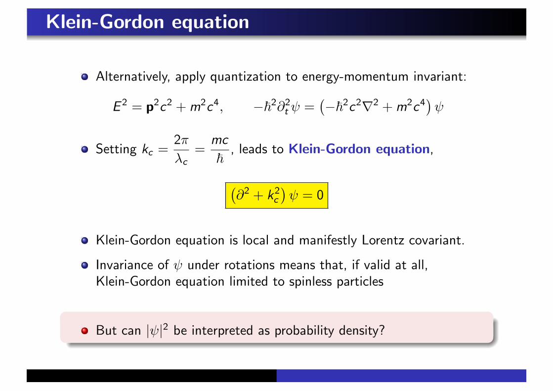
Alternatively, apply quantization to energy-momentum invariant:
E 2 = p2c2 + m2c4, $!2%2t & =
-$!2c2)2 + m2c4
.&
Setting kc =2'
"c=
mc
! , leads to Klein-Gordon equation,
-%2 + k2
c
.& = 0
Klein-Gordon equation is local and manifestly Lorentz covariant.
Invariance of & under rotations means that, if valid at all,Klein-Gordon equation limited to spinless particles
But can |&|2 be interpreted as probability density?

Klein-Gordon equation: Probabilities
Probabilities? Take lesson from non-relativistic quantum mechanics:
&%
Schrodinger eqn.) *' (+
i!%t +!2)2
2m
,& = 0,
c.c.) *' (
&
+$i!%t +
!2)2
2m
,&% = 0
i.e. %t |&|2 $ i!
2m) · (&%)& $ &)&%) = 0
cf. continuity relation – conservation of probability: %t( +) · j = 0
( = |&|2, j = $i!
2m(&%)& $ &)&%)

Klein-Gordon equation: Probabilities
Applied to KG equation: &%+
1
c2%2
t $)2 + k2c
,& = 0
!2%t (&%%t& $ &%t&%)$ !2c2) · (&%)& $ &)&%) = 0
cf. continuity relation – conservation of probability: %t( +) · j = 0.
( = i!
2mc2(&%%t& $ &%t&
%) , j = $i!
2m(&%)& $ &)&%)
With 4-current jµ = ((c , j), continuity relation %µjµ = 0.
i.e. Klein-Gordon density is the time-like component of a 4-vector.
Klein-Gordon equation: viability?
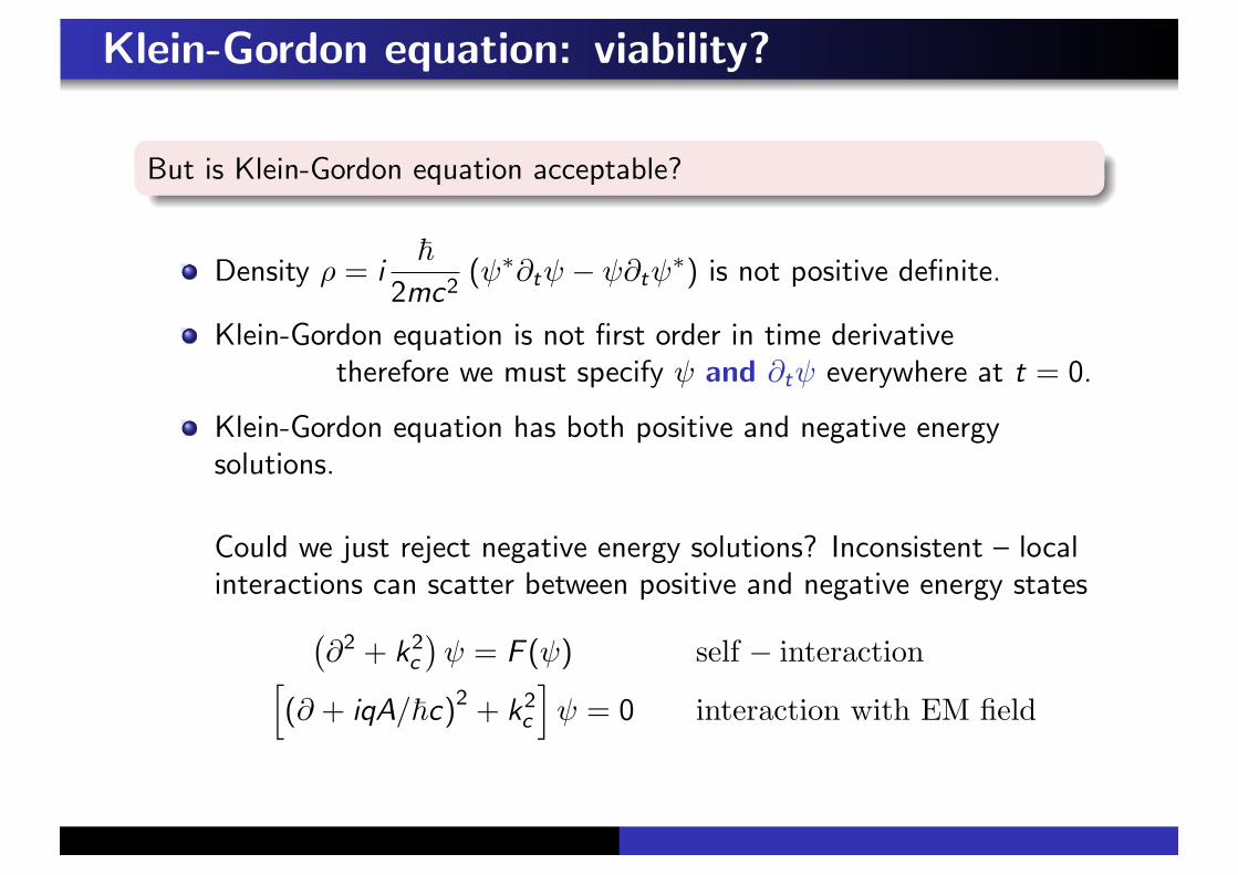
But is Klein-Gordon equation acceptable?
Density ( = i!
2mc2(&%%t& $ &%t&
%) is not positive definite.
Klein-Gordon equation is not first order in time derivativetherefore we must specify & and %t& everywhere at t = 0.
Klein-Gordon equation has both positive and negative energysolutions.
Could we just reject negative energy solutions? Inconsistent – localinteractions can scatter between positive and negative energy states
-%2 + k2
c
.& = F (&) self $ interaction
1(% + iqA/!c)2 + k2
c
2& = 0 interaction with EM field

Relativistic quantum mechanics: summary
When the kinetic energy of particles become comparable to restmass energy, p ! mc particles enter regime where relativity intrudeson quantum mechanics.
At these energy scales qualitatively new phenomena emerge:
e.g. particle production, existence of antiparticles, etc.
By applying canonical quantization procedure to energy-momentuminvariant, we are led to the Klein-Gordon equation,
(%2 + k2c )& = 0
where " ="c
2'=
!mc
denotes the Compton wavelength.
However, the Klein-Gordon equation does not lead to a positivedefinite probability density and admits positive and negative energysolutions – these features led to it being abandoned as a viablecandidate for a relativistic quantum mechanical theory.

Lecture 23Relativistic Quantum Mechanics:
Dirac equation

Relativistic quantum mechanics: outline
1 Special relativity (revision and notation)
2 Klein-Gordon equation
3 Dirac equation
4 Quantum mechanical spin
5 Solutions of the Dirac equation
6 Relativistic quantum field theories
7 Recovery of non-relativistic limit

Dirac Equation
Dirac placed emphasis on two constraints:
1 Relativistic equation must be first order in time derivative (andtherefore proportional to %µ = (%t/c ,))).
2 Elements of wavefunction must obey Klein-Gordon equation.
Dirac’s approach was to try to factorize Klein-Gordon equation:(%2 + m2)& = 0 (where henceforth we set ! = c = 1)
($i!!%! $m)(i!µ%µ $m)& = 0
i.e. with pµ = i%µ
(!µpµ $m) & = 0
Dirac Equation
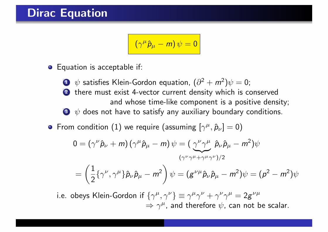
(!µpµ $m) & = 0
Equation is acceptable if:
1 & satisfies Klein-Gordon equation, (%2 + m2)& = 0;2 there must exist 4-vector current density which is conserved
and whose time-like component is a positive density;3 & does not have to satisfy any auxiliary boundary conditions.
From condition (1) we require (assuming [!µ, p! ] = 0)
0 = (!! p! + m) (!µpµ $m) & = ( !!!µ
' () *(%!%µ+%µ%!)/2
p! pµ $m2)&
=
+1
2{!! , !µ}p! pµ $m2
,& = (g!µp! pµ $m2)& = (p2 $m2)&
i.e. obeys Klein-Gordon if {!µ, !!} # !µ!! + !!!µ = 2g!µ
* !µ, and therefore &, can not be scalar.

Dirac Equation: Hamiltonian formulation
(!µpµ $m) & = 0, {!µ, !!} = 2g!µ
To bring Dirac equation to the form i%t& = H&, consider
!0(!µpµ $m)& = !0(!0p0 $ ! · p$m)& = 0
Since (!0)2 # 12{!
0, !0} = g00 = I,
!0(!µpµ $m)& = i%t& $ !0! · p& $m!0& = 0
i.e. Dirac equation can be written as i%t& = H& with
H = " · p + )m, " = !0!, ) = !0
Using identity {!µ, !!} = 2gµ! ,
)2 = I, {", )} = 0, {*i , *j} = 2#ij (exercise)

Dirac Equation: ! matrices
i%t& = H&, H = " · p + )m, " = !0!, ) = !0
Hermiticity of H assured if "† = ", and )† = ), i.e.
(!0!)† # !†!0† = !0!, and !0† = !0
So we obtain the defining properties of Dirac ! matrices,
!µ† = !0!µ!0, {!µ, !!} = 2gµ!
Since space-time is four-dimensional, ! must be of dimension atleast 4+ 4 – & has at least four components.
However, 4-component wavefunction & does not transform as4-vector – it is known as a spinor (or bispinor).

Dirac Equation: ! matrices
!µ† = !0!µ!0, {!µ, !!} = 2gµ!
From the defining properties, there are several possiblerepresentations of ! matrices. In the Dirac/Pauli representation:
!0 =
+I2 00 $I2
,, ! =
+0 #$# 0
,
# – Pauli spin matrices
+i+j = #ij + i,ijk+k , +i† = +i
e.g., +1 =
+0 11 0
,, +2 =
+0 $ii 0
,, +3 =
+1 00 $1
,
So, in Dirac/Pauli representation,
" = !0! =
+0 ## 0
,, ) = !0 =
+I2 00 $I2
,

Dirac Equation: conjugation, density and current
(!µpµ $m) & = 0, !µ† = !0!µ!0
Applying complex conjugation to Dirac equation
[(!µpµ $m)&]† = &†3$i!†
µ,$% µ $m
4= 0, &†,$% µ # (%µ&)†
Since (!0)2 = I, we can write,
0 = &†!0
' () *&
($i !0!†µ
' () *!µ!0
,$% µ $m!0) = $&
3i!µ,$% µ + m
4!0
Introducing Feynman ‘slash’ notation -a # !µaµ, obtain conjugateform of Dirac equation
&(i,$-% + m) = 0

Dirac Equation: conjugation, density and current
&(i,$-% + m) = 0, -% = !µ%µ
The, combining the Dirac equation, (i$&-% $m)& = 0 with its
conjugate, we have &(i,$-% + m)& = 0 = $&(i
$&-% $m)&, i.e.
&3,$-% +
$&-%
4& = %µ(&!µ&' () *
jµ
) = 0
We therefore identify jµ = ((, j) = (&†&,&†"&) as the 4-current.
So, in contrast to the Klein-Gordon equation, the density( = j0 = &†& is, as required, positive definite.
Motivated by this triumph(!), let us now consider what constraintsrelativistic covariance imposes and what consequences follow.

Relativistic covariance
If &(x) obeys the Dirac equation its counterpart &!(x !) in a LTframe x !! = "!
µxµ, must obey the Dirac equation,+
i!! %
%x !!$m
,&!(x !) = 0
If observer can reconstruct &!(x !) from &(x) there must exist alocal (linear) transformation,
&!(x !) = S(")&(x)
where S(") is a 4+ 4 matrix, i.e.
S(")
+i!µ %x!
%x !µ("$1)!
µS(")!!S$1(")!! %
%x!$m
,S(")&(x) = 0
Compatible with Dirac equation if S(")!!S$1(") = ("$1)!µ!µ

Relativistic covariance
&!(x !) = S(")&(x), S(")!!S$1(") = ("$1)!µ!µ
But how do we determine S(")? For an infinitesimal (i.e. properorthochronous) LT
"µ! = #µ
! + $µ! , ("$1)µ
! = #µ! $ $µ
! + · · ·
(recall that generators, $µ! = $$!µ, are antisymmetric).
This allows us to form the Taylor expansion of S("):
S(") # S(I + $) = S(I)'()*I
+
+%S
%$
,
µ!' () *
$ i
4#µ!
$µ! + O($2)
where #µ! = $#!µ (follows from antisymmetry of $) is a matrix inbispinor space, and $µ! is a number.

Relativistic covariance
S(") = I$ i
4#µ!$µ! + · · · , S$1(") = I +
i
4#µ!$µ! + · · ·
Requiring that S(")!!S$1(") = ("$1)!µ!µ, a little bit of algebra
(see problem set/handout) shows that matrices #µ! must obey therelation,
[#µ&, !! ] = 2i-!µ#!
& $ !&#!µ
.
This equation is satisfied by (exercise)
##$ =i
2[!#, !$]
In summary, under set of infinitesimal Lorentz transformation,x ! = "x , where " = I + $, relativistic covariance of Dirac equationdemands that wavefunction transforms as &!(x !) = S(")& whereS(") = I$ i
4#µ!$µ! + O($2) and #µ! = i2 [!µ, !! ].

Relativistic covariance
S(") = I$ i
4#µ!$µ! + · · ·
“Finite” transformations (i.e. non-infinitesimal) generated by
S(") = exp
5$ i
4##$$#$
6, $#$ = "#$ $ g#$
1 Transformations involving unitary matrices S("), whereS†S = I translate to spatial rotations.
2 Transformations involving Hermitian matrices S("), whereS† = S translate to Lorentz boosts.
So what?? What are the consequences of relativistic covariance?
Angular momentum and spin
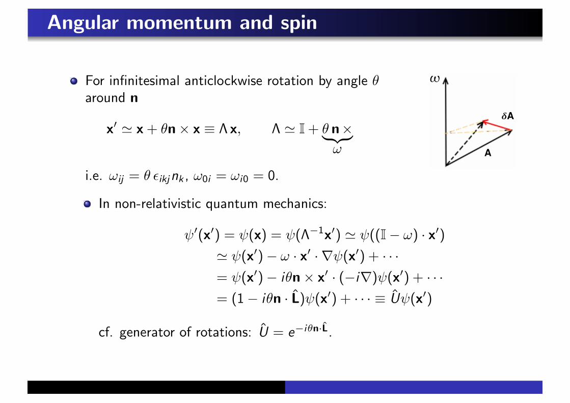
For infinitesimal anticlockwise rotation by angle -around n
x! . x + -n+ x # " x, " . I + - n+' () *$
i.e. $ij = - ,ikjnk , $0i = $i0 = 0.
In non-relativistic quantum mechanics:
&!(x!) = &(x) = &("$1x!) . &((I$ $) · x!). &(x!)$ $ · x! ·)&(x!) + · · ·= &(x!)$ i-n+ x! · ($i))&(x!) + · · ·= (1$ i-n · L)&(x!) + · · · # U&(x!)
cf. generator of rotations: U = e$i'n·L.
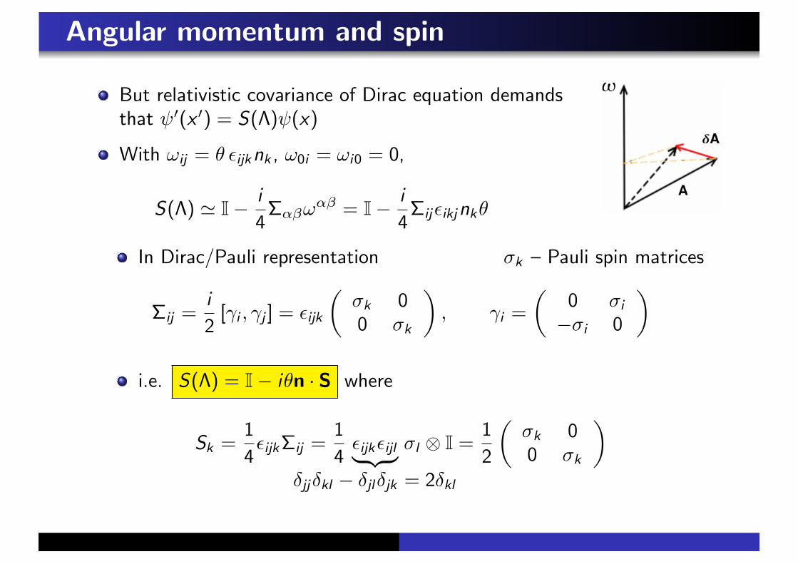
Angular momentum and spin
But relativistic covariance of Dirac equation demandsthat &!(x !) = S(")&(x)
With $ij = - ,ijknk , $0i = $i0 = 0,
S(") . I$ i
4##$$#$ = I$ i
4#ij,ikjnk-
In Dirac/Pauli representation +k – Pauli spin matrices
#ij =i
2[!i , !j ] = ,ijk
++k 00 +k
,, !i =
+0 +i
$+i 0
,
i.e. S(") = I$ i-n · S where
Sk =1
4,ijk#ij =
1
4,ijk,ijl' () *
#jj#kl $ #jl#jk = 2#kl
+l / I =1
2
++k 00 +k
,

Angular momentum and spin
Altogether, combining components of transformation,
&!(x !) =
I$ i-n · S)*'(S(") &(x"$1x !)' () *
(I$ i-n · L)&(x !)
. (I$ i-n · (S + L))&(x !)
we obtain
&!(x !) = S(")&("$1x !) . (1$ i-n · J)&(x !)
where J = L + S represents total angular momentum.
Intrinsic contribution to angular momentum known as spin.
[Si ,Sj ] = i,ijkSk , (Si )2 =
1
4for each i
Dirac equation is relativistic wave equation for spin 1/2 particles.

Parity
So far we have only dealt with the subgroup of properorthochronous Lorentz transformations, L"
+.
Taking into account Parity, Pµ! =
!
""#
1$1
$1$1
$
%%&
relativistic covariance demands S(")!!S$1(") = ("$1)!µ!µ
S$1(P)!0S(P) = !0, S$1(P)! iS(P) = $! i
achieved if S(P) = !0e i(, where . denotes arbitrary phase.
But since P2 = I, e i( = 1 or $1
&!(x !) = S(P)&("$1x !) = /!0&(Px !)
where / = ±1 — intrinsic parity of the particle
Lecture 24
Relativistic Quantum Mechanics:Solutions of the Dirac equation

Relativistic quantum mechanics: outline
1 Special relativity (revision and notation)
2 Klein-Gordon equation
3 Dirac equation
4 Quantum mechanical spin
5 Solutions of the Dirac equation
6 Relativistic quantum field theories
7 Recovery of non-relativistic limit

Free particle solutions of Dirac Equation
(-p $m)& = 0, -p = i!µ%µ
Free particle solution of Dirac equation is a plane wave:
&(x) = e$ip·xu(p) = e$iEt+ip·xu(p)
where u(p) is the bispinor amplitude.
Since components of & obey KG equation, (pµpµ $m2)& = 0,
(p0)2 $ p2 $m2 = 0, E # p0 = ±
7p2 + m2
So, once again, as with Klein-Gordon equation we encounterpositive and negative energy solutions!!

Free particle solutions of Dirac Equation
&(x) = e$ip·xu(p) = e$iEt+ip·xu(p)
What about bispinor amplitude, u(p)?
In Dirac/Pauli representation,
!0 =
+I2
$I2
,, ! =
+#
$#
,
the components of the bispinor obeys the condition,
(!µpµ $m)u(p) =
+p0 $m $# · p# · p $p0 $m
,u(p) = 0
i.e. bispinor elements:
u(p) =
+0/
,,
8(p0 $m)0 = + · p/+ · p0 = (p0 + m)/

Free particle solutions of the Dirac Equation
u(p) =
+0/
,,
8(p0 $m)0 = + · p/+ · p0 = (p0 + m)/
Consistent when (p0)2 = p2 + m2 and / =# · p
p0 + m0
u(r)(p) = N(p)
91(r)
# · pp0 + m
1(r)
:
where 1(r) are a pair of orthogonal two-component vectors withindex r = 1, 2, and N(p) is normalization.
Helicity: Eigenvalue of spin projected along direction of motion
1
2# · p
|p|1(±) # S · p
|p|1(±) = ±1
21(±)
e.g. if p = p e3, 1(+) = (1, 0), 1($) = (0, 1)
Free particle solutions of the Dirac Equation
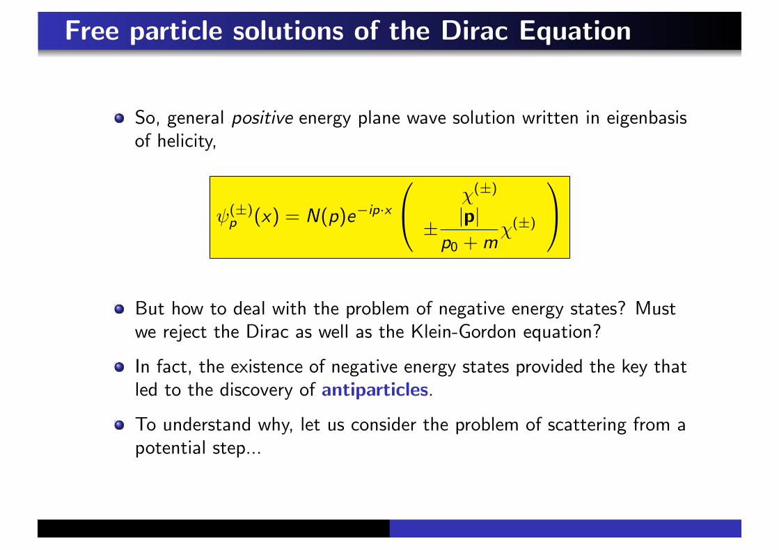
So, general positive energy plane wave solution written in eigenbasisof helicity,
&(±)p (x) = N(p)e$ip·x
!
#1(±)
± |p|p0 + m
1(±)
$
&
But how to deal with the problem of negative energy states? Mustwe reject the Dirac as well as the Klein-Gordon equation?
In fact, the existence of negative energy states provided the key thatled to the discovery of antiparticles.
To understand why, let us consider the problem of scattering from apotential step...

Klein paradox and antiparticles
Consider plane wave, unit amplitude, energy E , momentum p e3,and spin 0 (1 = (1, 0)) incident on potential barrier V (x) = V -(x3)
&in = e$ip0t+ipx3
91(+)
p
p0 + m1(+)
:
At barrier, spin is conserved, component r is reflected (E , $p e3),and component t is transmitted (E ! = E $ V , p! e3)
From Klein-Gordon condition (energy-momentum invariant):p2
0 # E 2 = p2 + m2 and p!02 # E !2 = p!2 + m2

Klein paradox and antiparticles
&in = e$ip0t+ipx3
91(+)
p
p0 + m1(+)
:
Boundary conditions: since Dirac equation is first order, require onlycontinuity of & at interface (cf. Schrodinger eqn.)
!
""#
10
p/(E + m)0
$
%%& + r
!
""#
10
$p/(E + m)0
$
%%& = t
!
""#
10
p!/(E ! + m)0
$
%%&
(helicity conserved in reflection)
Equating (generically complex) coe$cients:
1 + r = t,p
E + m(1$ r) =
p!
E ! + mt

Klein paradox and antiparticles
1 + r = t (1),p
E + m(1$ r) =
p!
E ! + mt (2)
From (2), 1$ r = 2t where
2 =p!
p
(E + m)
(E ! + m)
Together with (1), (1 + 2)t = 2
t =2
1 + 2,
1 + r
1$ r=
1
2, r =
1$ 2
1 + 2
Interpret solution by studying vector current: j = &!& = &†"&
j3 = &†*3&, *3 = !0!3 =
++3
+3
,

Klein paradox and antiparticles
j3 = &†+
+3
+3
,&
(Up to overall normalization) the incident, transmitted and reflectedcurrents given by,
j (i)3 =-
1 0 pE+m 0
. +0 +3
+3 0
,!
""#
10p
E+m0
$
%%& =2p
E + m,
j (t)3 =1
E ! + m(p! + p!%)|t|2, j (r)3 = $ 2p
E + m|r |2
where we note that, depending on height of the potential, p! maybe complex (cf. NRQM).
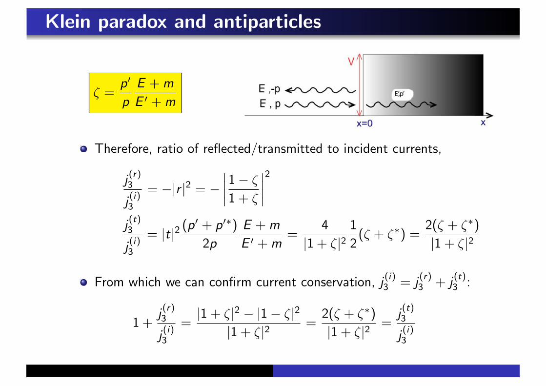
Klein paradox and antiparticles
2 =p!
p
E + m
E ! + m
Therefore, ratio of reflected/transmitted to incident currents,
j (r)3
j (i)3
= $|r |2 = $;;;;1$ 2
1 + 2
;;;;2
j (t)3
j (i)3
= |t|2 (p! + p!%)
2p
E + m
E ! + m=
4
|1 + 2|21
2(2 + 2%) =
2(2 + 2%)
|1 + 2|2
From which we can confirm current conservation, j (i)3 = j (r)3 + j (t)3 :
1 +j (r)3
j (i)3
=|1 + 2|2 $ |1$ 2|2
|1 + 2|2 =2(2 + 2%)
|1 + 2|2 =j (t)3
j (i)3

Klein paradox and antiparticles
j (r)3
j (i)3
= $|r |2 = $;;;;1$ 2
1 + 2
;;;;2
Three distinct regimes in energy:
1 E ! # (E $ V ) > m:
i.e. p!2 = E !2 $m2 > 0, p! > 0 (beam propagates to right).
Therefore 2 # p!
p
E + m
E ! + m> 0 and real; |j (r)3 | < |j (i)3 | as expected,
i.e. for E ! > m, as in non-relativistic quantum mechanics, some ofthe beam is reflected and some transmitted.
2 m > E ! > $m:
i.e. p!2 = E !2 $m2 < 0, p! pure imaginary.
Particles have insu$cient energy to surmount potential barrier.
Therefore, 2 # p!
p
E + m
E ! + mpure imaginary, |j (r)3 | = |j (i)3 |.
i.e. all beam is reflected; & has evanescant decays on the right handside of the barrier (cf. NRQM).
3 E ! = E $ V < $m:
i.e. step height V > E +m 1 2m larger than twice rest mass energy.
p!2 = E !2 $m2 > 0, p! > 0 (beam propagates to the right)
But 2 =p!
p
(E + m)
(E ! + m)< 0 real!
Therefore |j (r)3 | > |j (i)3 |!! – more current is reflected than is incident– Klein Paradox (also holds for Klein-Gordon equation).
But particle current conserved – it is as though an additional beamof particles were incident from right.

Klein paradox and antiparticles
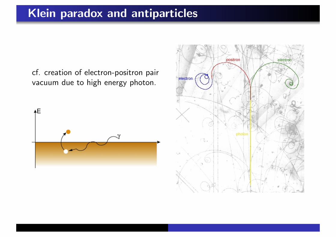
Physical Interpretation:
“Particles” from right should be interpreted as antiparticlespropagating to right
i.e. incoming beam stimulates emission of particle/antiparticle pairsat barrier.
Particles combine with reflected to beam to create current to leftthat is larger than incident current while antiparticles propagate tothe right in the barrier region.
Klein paradox and antiparticles
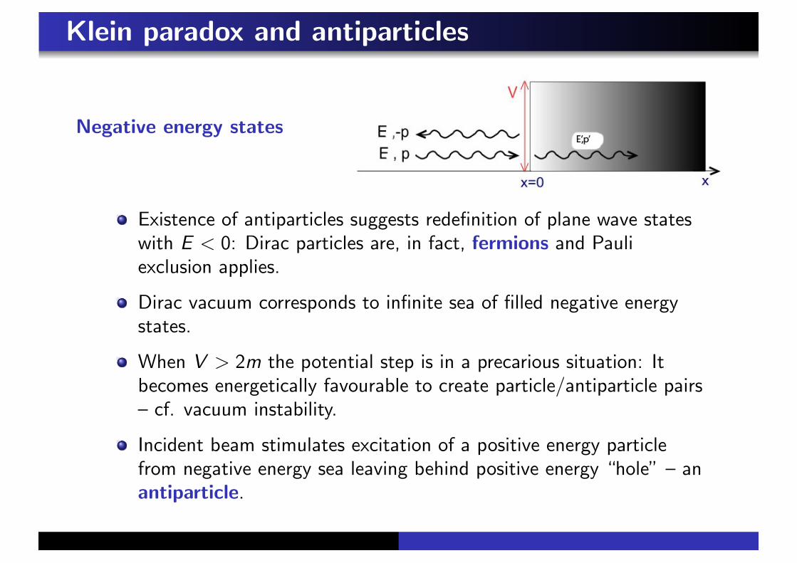
Negative energy states
Existence of antiparticles suggests redefinition of plane wave stateswith E < 0: Dirac particles are, in fact, fermions and Pauliexclusion applies.
Dirac vacuum corresponds to infinite sea of filled negative energystates.
When V > 2m the potential step is in a precarious situation: Itbecomes energetically favourable to create particle/antiparticle pairs– cf. vacuum instability.
Incident beam stimulates excitation of a positive energy particlefrom negative energy sea leaving behind positive energy “hole” – anantiparticle.
Klein paradox and antiparticles
cf. creation of electron-positron pairvacuum due to high energy photon.
Klein paradox and antiparticles
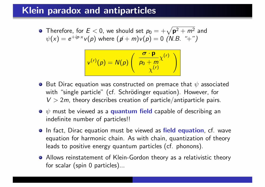
Therefore, for E < 0, we should set p0 = +7
p2 + m2 and&(x) = e+ip·xv(p) where (-p + m)v(p) = 0 (N.B. “+”)
v (r)(p) = N(p)
9 # · pp0 + m
1(r)
1(r)
:
But Dirac equation was constructed on premace that & associatedwith “single particle” (cf. Schrodinger equation). However, forV > 2m, theory describes creation of particle/antiparticle pairs.
& must be viewed as a quantum field capable of describing anindefinite number of particles!!
In fact, Dirac equation must be viewed as field equation, cf. waveequation for harmonic chain. As with chain, quantization of theoryleads to positive energy quantum particles (cf. phonons).
Allows reinstatement of Klein-Gordon theory as a relativistic theoryfor scalar (spin 0 particles)...

Quantization of Klein-Gordon field
Klein-Gordon equation abandoned as candidate for relativistictheory on basis that (i) it admitted negative energy solutions, and(ii) probability density was not positive definite.
But Klein paradox suggests reinterpretation of Dirac wavefunctionas a quantum field.
If . were a classical field, Klein-Gordon equation, (%2 $m2). = 0would be associated with Lagrangian density,
L =1
2%µ.%µ.$ 1
2m2.2
Defining canonical momentum, '(x) = %(L = .(x)
H = '.$ L =1
2
/'2 + ().)2 + m2.2
0
H is +ve definite! i.e. if quantized, only +ve energies appear.
Quantization of Klein-Gordon field
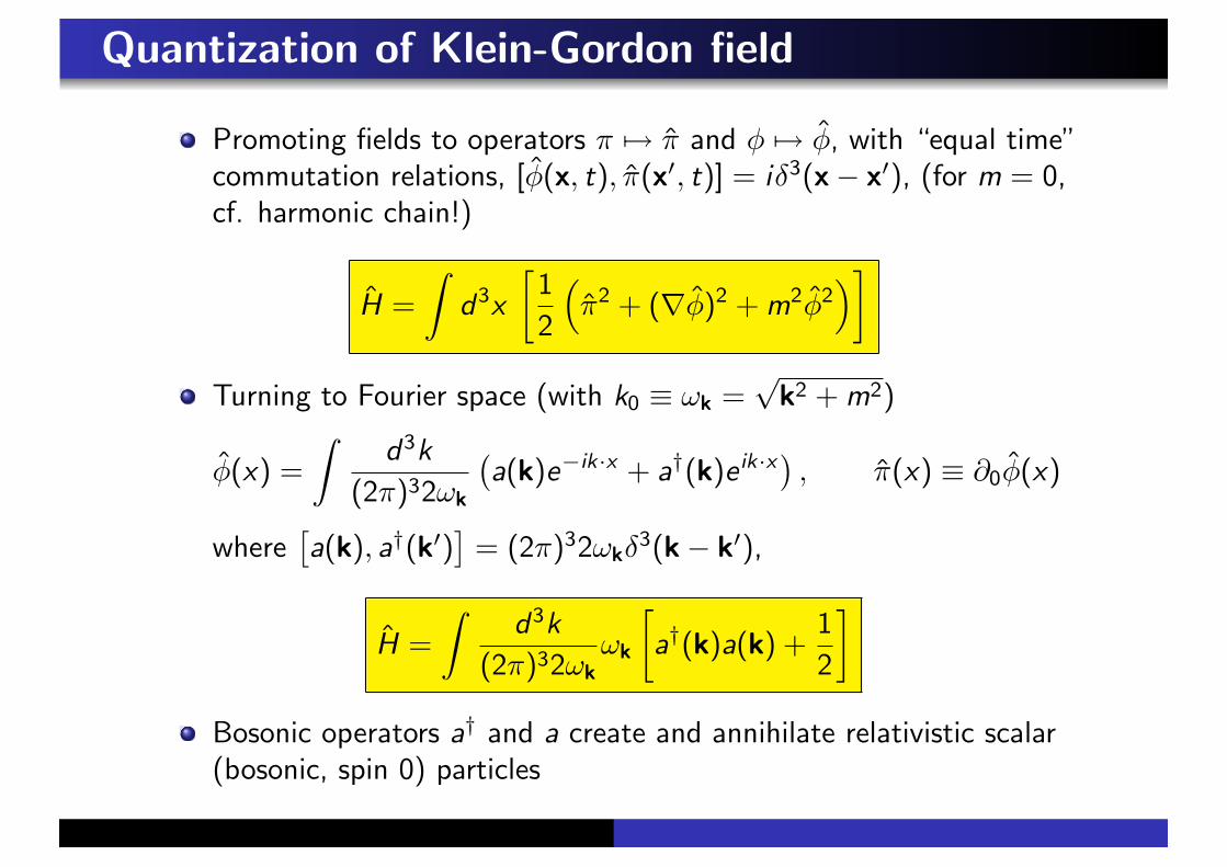
Promoting fields to operators ' %& ' and . %& ., with “equal time”commutation relations, [.(x, t), '(x!, t)] = i#3(x$ x!), (for m = 0,cf. harmonic chain!)
H =
<d3x
51
2
3'2 + ().)2 + m2.2
46
Turning to Fourier space (with k0 # $k =2
k2 + m2)
.(x) =
<d3k
(2')32$k
-a(k)e$ik·x + a†(k)e ik·x. , '(x) # %0.(x)
where/a(k), a†(k!)
0= (2')32$k#3(k$ k!),
H =
<d3k
(2')32$k$k
5a†(k)a(k) +
1
2
6
Bosonic operators a† and a create and annihilate relativistic scalar(bosonic, spin 0) particles

Quantization of Dirac field
Dirac equation associated with Lagrangian density,
L = & (i!µ%µ $m)&, i.e. %)L = (i!µ%µ $m) & = 0
With momentum ' = %)L = i&!0 = i&†, Hamiltonian density
H = '& $ L = &i!0%0& $ L = & ($i! ·)+ m) &
Once again, we can follow using canonical quantization procedure,promoting fields to operators – but, in this case, one must imposeequal time anti-commutation relations,
{&#(x, t), '(x!, t)} # &#(x, t)'$(x!, t) + '$(x, t)&#(x!, t)
= i#3(x$ x!)##$

Quantization of Dirac field
Turning to Fourier space (with k0 # $k =2
k2 + m2)
&(x) =2=
r=1
<d3k
(2')32$k
1ar (k)u(r)(k)e$ik·x + b†r (k)v (r)(k)e ik·x
2
with equal time anti-commutation relations (hallmark of fermions!)>ar (k), a†s (k
!)?
=>br (k), b†s (k
!)?
= (2')32$k#rs#3(k$ k!)
>a†r (k), a†s (k
!)?
=>b†r (k), b†s (k
!)?
= 0
which accommdates Pauli exclusion a†r (k)2 = 0(!), obtain
H =2=
r=1
<d3k
(2')32$k$k
/a†r (k)ar (k) + b†r (k)br (k)
0
Physically a(k)u(r)(k)e$ik·x annihilates +ve energy fermion particle(helicity r), and b†(k)v (r)(k)e ik·x creates a +ve energy antiparticle.

Low energy limit of the Dirac equation
Previously, we have explored the relativistic (fine-structure)corrections to the hydrogen atom. At the time, we alluded to theseas the leading relativistic contributions to the Dirac theory.
In the following section, we will explore how these correctionsemerge from relativistic formulation.
But first, we must consider interaction of charged particle withelectromagnetic field.
As with non-relativistic quantum mechanics, interaction of Diracparticle of charge q (q = $e for electron) with EM field defined byminimal substitution, pµ %$& pµ $ qAµ, where Aµ = (.,A), i.e.
(-p $ q -A$m)& = 0

Low energy limit of the Dirac equation
For particle moving in potential (.,A), stationary form of DiracHamiltonian given by H& = E& where, restoring factors of ! and c ,
H = c" · (p$ qA) + mc2) + q.
=
+mc2 + q. c# · (p$ qA)
c# · (p$ qA) $mc2 + q.
,
To develop non-relativistic limit, consider bispinor &T = (&a, &b),where the elements obey coupled equations,
(mc2 + q.)&a + c# · (p$ qA)&b = E&a
c# · (p$ qA)&a $ (mc2 $ q.)&b = E&b
If we define energy shift over rest mass energy, W = E $mc2,
&b =1
2mc2 + W $ q.c# · (p$ qA)&a

Low energy limit of the Dirac equation
&b =1
2mc2 + W $ q.c# · (p$ qA)&a
In the non-relativistic limit, W ( mc2 and we can develop anexpansion in v/c . At leading order, &b . 1
2mc2 c# · (p$ qA)&a.
Substituted into first equation, obtain Pauli equationHNR&a = W&a where, defining V = q.,
HNR =1
2m[# · (p$ qA)]2 + V .
Making use of Pauli matrix identity +i+j = #ij + i,ijk+k ,
HNR =1
2m(p$ qA)2 $ q!
2m# · ()+ A) + V
i.e. spin magnetic moment,
µS =q!2m
# = gq
2mS, with gyromagnetic ratio, g = 2.

Low energy limit of the Dirac equation
&b =1
2mc2 + W $ Vc# · (p$ qA)&a
Taking into account the leading order (in v/c) correction (withA = 0 for simplicity), we have
&b .1
2mc2
+1$ W $ V
2mc2
,c# · p&a
Then substituted into the second bispinor equation (and taking intoaccount correction from normalization) we find
H . p2
2m+ V $ p4
8m3c2' () *
k.e.
+1
2m2c2S · ()V )+ p
' () *spin$orbit coupling
+!2
8m2c2()2V )
' () *Darwin term

Synopsis: (mostly revision) Lectures 1-4ish
1 Foundations of quantum physics:†Historical background; wave mechanics to Schrodinger equation.
2 Quantum mechanics in one dimension:
Unbound particles: potential step, barriers and tunneling; boundstates: rectangular well, #-function well; †Kronig-Penney model .
3 Operator methods:
Uncertainty principle; time evolution operator; Ehrenfest’s theorem;†symmetries in quantum mechanics; Heisenberg representation;quantum harmonic oscillator; †coherent states.
4 Quantum mechanics in more than one dimension:
Rigid rotor; angular momentum; raising and lowering operators;representations; central potential; atomic hydrogen.
† non-examinable *in this course*.
Synopsis: Lectures 5-10
5 Charged particle in an electromagnetic field:
Classical and quantum mechanics of particle in a field; normalZeeman e%ect; gauge invariance and the Aharonov-Bohm e%ect;Landau levels, †Quantum Hall e%ect.
6 Spin:
Stern-Gerlach experiment; spinors, spin operators and Paulimatrices; spin precession in a magnetic field; parametric resonance;addition of angular momenta.
7 Time-independent perturbation theory:
Perturbation series; first and second order expansion; degenerateperturbation theory; Stark e%ect; nearly free electron model.
8 Variational and WKB method:
Variational method: ground state energy and eigenfunctions;application to helium; †Semiclassics and the WKB method.
† non-examinable *in this course*.

Synopsis: Lectures 11-15
9 Identical particles:
Particle indistinguishability and quantum statistics; space and spinwavefunctions; consequences of particle statistics; ideal quantumgases; †degeneracy pressure in neutron stars; Bose-Einsteincondensation in ultracold atomic gases.
10 Atomic structure:
Relativistic corrections – spin-orbit coupling; Darwin term; Lambshift; hyperfine structure. Multi-electron atoms; Helium; Hartreeapproximation †and beyond; Hund’s rule; periodic table; LS and jjcoupling schemes; atomic spectra; Zeeman e%ect.
11 Molecular structure:
Born-Oppenheimer approximation; H+2 ion; H2 molecule; ionic and
covalent bonding; LCAO method; from molecules to solids;†application of LCAO method to graphene; molecular spectra;rotation and vibrational transitions.
† non-examinable *in this course*.

Synopsis: Lectures 16-19
12 Field theory: from phonons to photons:
From particles to fields: classical field theory of harmonic atomicchain; quantization of atomic chain; phonons; classical theory of theEM field; †waveguide; quantization of the EM field and photons.
13 Time-dependent perturbation theory:
Rabi oscillations in two level systems; perturbation series; suddenapproximation; harmonic perturbations and Fermi’s Golden rule.
14 Radiative transitions:
Light-matter interaction; spontaneous emission; absorption andstimulated emission; Einstein’s A and B coe$cents; dipoleapproximation; selection rules; lasers.
† non-examinable *in this course*.

Synopsis: Lectures 20-24
15 Scattering theory†Elastic and inelastic scattering; †method of particle waves; †Bornseries expansion; Born approximation from Fermi’s Golden rule;†scattering of identical particles.
16 Relativistic quantum mechanics:†Klein-Gordon equation; †Dirac equation; †relativistic covariance andspin; †free relativistic particles and the Klein paradox; †antiparticles;†coupling to EM field: †minimal coupling and the connection tonon-relativistic quantum mechanics; †field quantization.
† non-examinable *in this course*.
Recommended