CPU Scheduling
Heechul Yun
1
Recap
• Four deadlock conditions:
– Mutual exclusion
– No preemption
– Hold and wait
– Circular wait
• Detection
• Avoidance
– Banker’s algorithm
2

Recap: Banker’s Algorithm1. Initialize Avail and Finish vectors
Avail = FreeResources;
For i = 1,2, …, n, Finish[i] = false
2. Find an index i such that Finish[i] == false AND
Max[i] – Alloc[i] Avail
If no such i exists, go to step 4
3. Avail = Avail + Alloc[i] , Finish[i] = trueGo to step 2
4. If Finish[i] == false, for some i, 1 i n,
(a) then the system is in deadlock state
(b) if Finish[i] == false, then Pi is deadlocked
FreeResources: resource vector [R1, R2] = [0,0]
Alloc[i]: process i’s allocated resource vector: Alloc[1] = [0,1], Alloc[2] = [1, 0]
Request[i]: process i’s requesting vector: Request[1] = [1,0]Request[2] = [0,0]
Max[i]: process i’s maximum resource demand vector
3

Administrative
• Midterm
– March 12, 2018
– Closed book, in-class
– Review class: March 9, 2018
4
Agenda
• Introduction to CPU scheduling
• Classical CPU scheduling algorithms
5

CPU Scheduling
• CPU scheduling is a policy to decide
– Which thread to run next?
– When to schedule the next thread?
– How long?
• Context switching is a mechanism
– To change the running thread
6
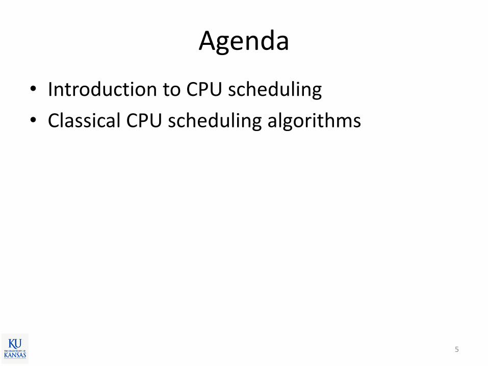
Assumption: CPU Bursts
• Execution model
– Program uses the CPU for a while and the does some I/O, back to use CPU, …, keep alternating
7
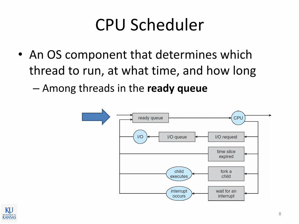
CPU Scheduler
• An OS component that determines which thread to run, at what time, and how long
– Among threads in the ready queue
8
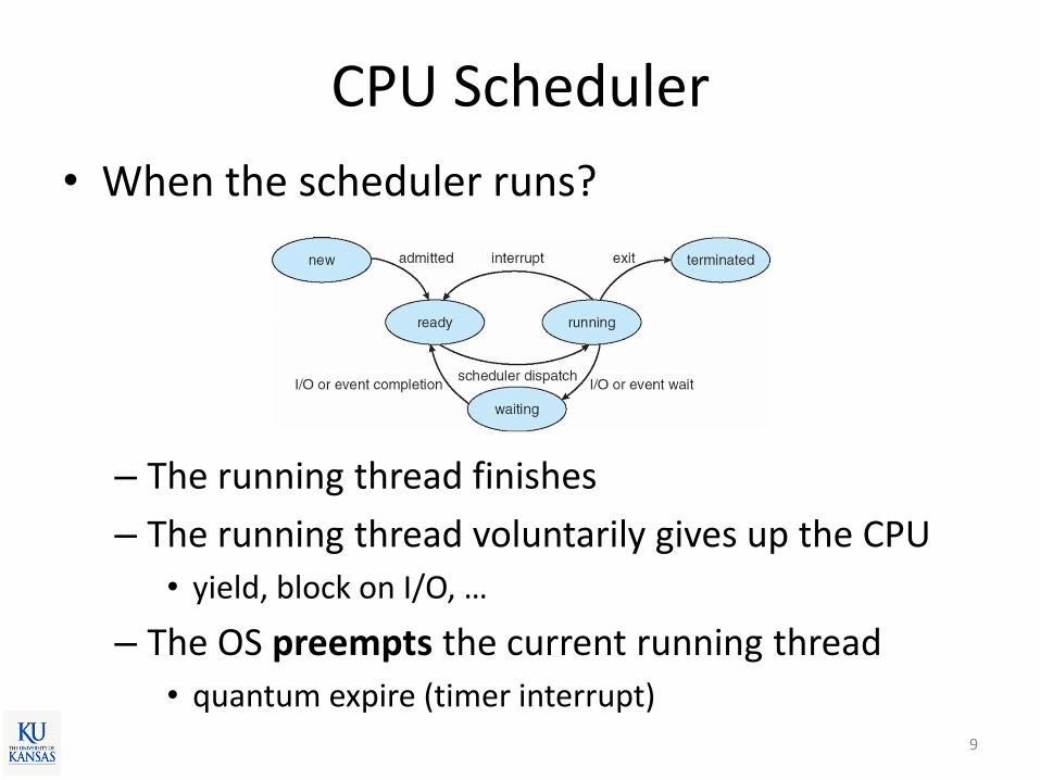
CPU Scheduler
• When the scheduler runs?
– The running thread finishes
– The running thread voluntarily gives up the CPU
• yield, block on I/O, …
– The OS preempts the current running thread
• quantum expire (timer interrupt)9

Performance Metrics for CPU Scheduling
• CPU utilization
– % of time the CPU is busy doing something
• Throughput
– #of jobs done / unit time
• Response time (Turn-around time)
– Time to complete a task (ready -> complete)
• Waiting time
– Time spent on waiting in the ready queue
• Scheduling latency
– Time to schedule a task (ready -> first scheduled)
10

Example
• Assumption: A, B, C are released at time 0
• The times of Process A
– Response time: 9
– Wait time: 5
– Sched. latency: 011
A B C A B C A C A C Time
sched. latency+ +wait time
response time
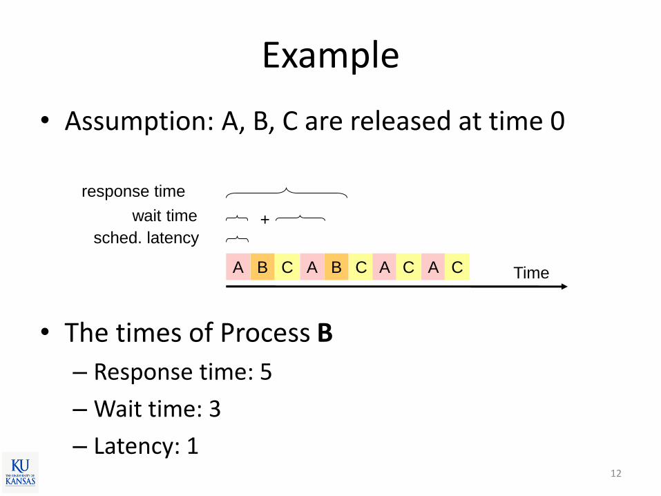
Example
• Assumption: A, B, C are released at time 0
• The times of Process B
– Response time: 5
– Wait time: 3
– Latency: 112
A B C A B C A C A C Time
sched. latency+wait time
response time

Example
• Assumption: A, B, C are released at time 0
• The times of Process C
– Response time: 10
– Wait time: 6
– Latency: 213
A B C A B C A C A C Time
sched. latency+ ++wait time
response time
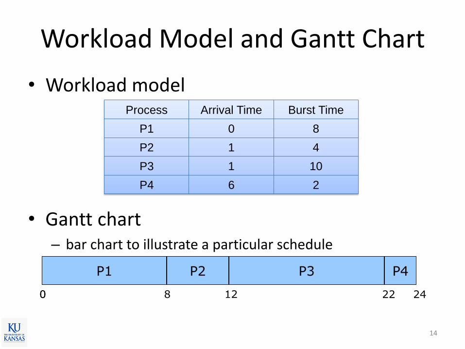
Workload Model and Gantt Chart
• Workload model
• Gantt chart– bar chart to illustrate a particular schedule
14
Process Arrival Time Burst Time
P1 0 8
P2 1 4
P3 1 10
P4 6 2
P1 P2 P3 P4
0 80 12 22 24
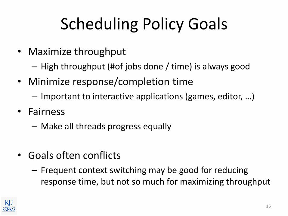
Scheduling Policy Goals
• Maximize throughput
– High throughput (#of jobs done / time) is always good
• Minimize response/completion time
– Important to interactive applications (games, editor, …)
• Fairness
– Make all threads progress equally
• Goals often conflicts
– Frequent context switching may be good for reducing response time, but not so much for maximizing throughput
15

First-Come, First-Served (FCFS)
• FCFS
– Assigns the CPU based on the order of the requests.
– Implemented using a FIFO queue.
16

FCFS
• Example
– Suppose that the processes arrive in the order: P1 , P2 , P3
– Waiting time? • P1 = 0; P2 = 24; P3 = 27
– Average waiting time• (0 + 24 + 27)/3 = 17
17
Process Arrival Time Burst Time
P1 0 24
P2 0 3
P3 0 3
P1 P2 P3
24 27 300

FCFS• Example 2
– Suppose that the processes arrive in the order: P2 , P3, P1
– Waiting time? • P1 = 6; P2 = 0; P3 = 3
– Average waiting time• (6 + 0 + 3)/3 = 3
– Much better than previous case performance varies greatly depending on the scheduling order
18
Process Arrival Time Burst Time
P1 0 24
P2 0 3
P3 0 3
P1P3P2
63 300
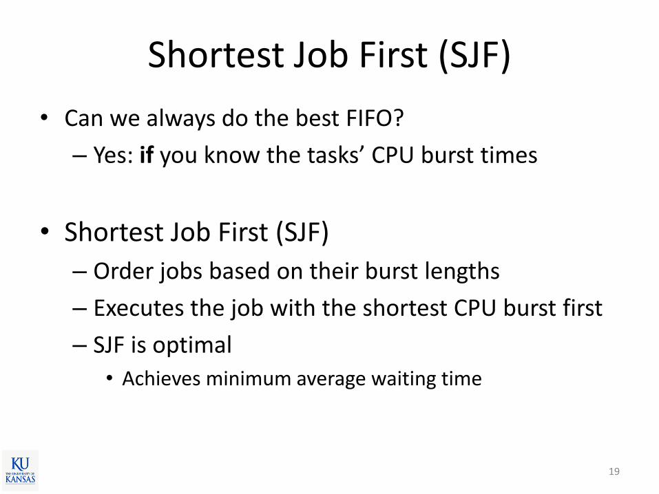
Shortest Job First (SJF)
• Can we always do the best FIFO?
– Yes: if you know the tasks’ CPU burst times
• Shortest Job First (SJF)
– Order jobs based on their burst lengths
– Executes the job with the shortest CPU burst first
– SJF is optimal
• Achieves minimum average waiting time
19
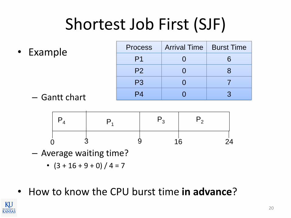
Shortest Job First (SJF)
• Example
– Gantt chart
– Average waiting time?• (3 + 16 + 9 + 0) / 4 = 7
• How to know the CPU burst time in advance?
20
Process Arrival Time Burst Time
P1 0 6
P2 0 8
P3 0 7
P4 0 3
P4P3P1
3 160 9
P2
24

Determining CPU Burst Length
• Can only estimate the length
– Next CPU burst similar to previous CPU bursts ?
– Predict based on the past history
• Exponential weighted moving average (EWMA)
– of past CPU bursts
21
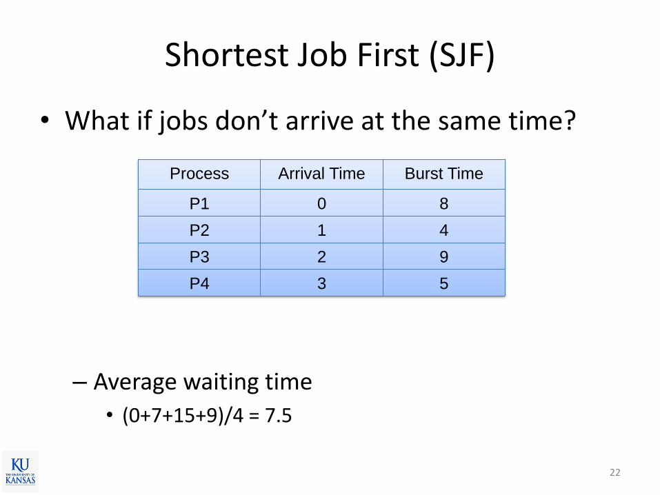
Shortest Job First (SJF)
• What if jobs don’t arrive at the same time?
– Average waiting time
• (0+7+15+9)/4 = 7.5
22
Process Arrival Time Burst Time
P1 0 8
P2 1 4
P3 2 9
P4 3 5
P2 P4P1 P3
0 8 12 17 26
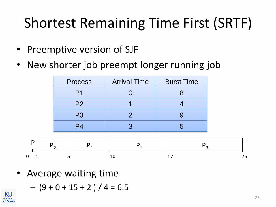
Shortest Remaining Time First (SRTF)
• Preemptive version of SJF
• New shorter job preempt longer running job
• Average waiting time
– (9 + 0 + 15 + 2 ) / 4 = 6.523
Process Arrival Time Burst Time
P1 0 8
P2 1 4
P3 2 9
P4 3 5
P1
P2 P4 P1 P3
0 1 5 10 17 26
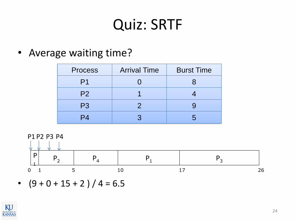
Quiz: SRTF
• Average waiting time?
• (9 + 0 + 15 + 2 ) / 4 = 6.5
24
Process Arrival Time Burst Time
P1 0 8
P2 1 4
P3 2 9
P4 3 5
P1
P2 P4 P1 P3
0 1 5 10 17 26
P1 P2 P3 P4
So Far…
• FIFO
– In the order of arrival
– Non-preemptive
• SJF
– Shortest job first.
– Non preemptive
• SRTF
– Preemptive version of SJF
25
Issues
• FIFO
– Bad average response time
• SJF/SRTF
– Good average response time
– IF you know or can predict the future
• Time-sharing systems
– Multiple users share a machine
– Need high interactivity low response time 26

Round-Robin (RR)
• FIFO with preemption
• Simple, fair, and easy to implement
• Algorithm
– Each job executes for a fixed time slice: quantum
– When quantum expires, the scheduler preempts the task
– Schedule the next job and continue...
27

Round-Robin (RR)
• Example
– Quantum size = 4
– Gantt chart
– Sched. Latency (between ready to first schedule)• P1: 0, P2: 4, P3: 7. average response time = (0+4+7)/3 = 3.67
– Waiting time• P1: 6, P2: 4, P3: 7. average waiting time = (6+4+7)/3 = 5.67
28
Process Burst Times
P1 24
P2 3
P3 3
P1 P2 P3 P1 P1 P1 P1 P1
0 4 7 10 14 18 22 26 30

How To Choose Quantum Size?
• Quantum length
– Too short high overhead (why?)
– Too long bad response time• Very long quantum FIFO
29
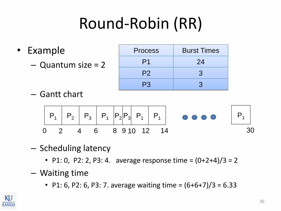
Round-Robin (RR)
• Example
– Quantum size = 2
– Gantt chart
– Scheduling latency• P1: 0, P2: 2, P3: 4. average response time = (0+2+4)/3 = 2
– Waiting time• P1: 6, P2: 6, P3: 7. average waiting time = (6+6+7)/3 = 6.33
30
Process Burst Times
P1 24
P2 3
P3 3
P1 P2 P3 P1 P2 P1 P1P3 P1
0 2 4 6 8 9 12 1410 30

Discussion
• Comparison between FCFS, SRTF(SJF), and RR
– What to choose for smallest average waiting time?
• SRTF (SFJ) is the optimal
– What to choose for better interactivity?
• RR with small time quantum (or SRTF)
– What to choose to minimize scheduling overhead?
• FCFS
31
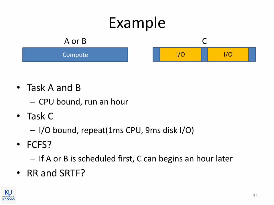
Example
• Task A and B
– CPU bound, run an hour
• Task C
– I/O bound, repeat(1ms CPU, 9ms disk I/O)
• FCFS?
– If A or B is scheduled first, C can begins an hour later
• RR and SRTF?
32
Compute I/O I/O
A or B C
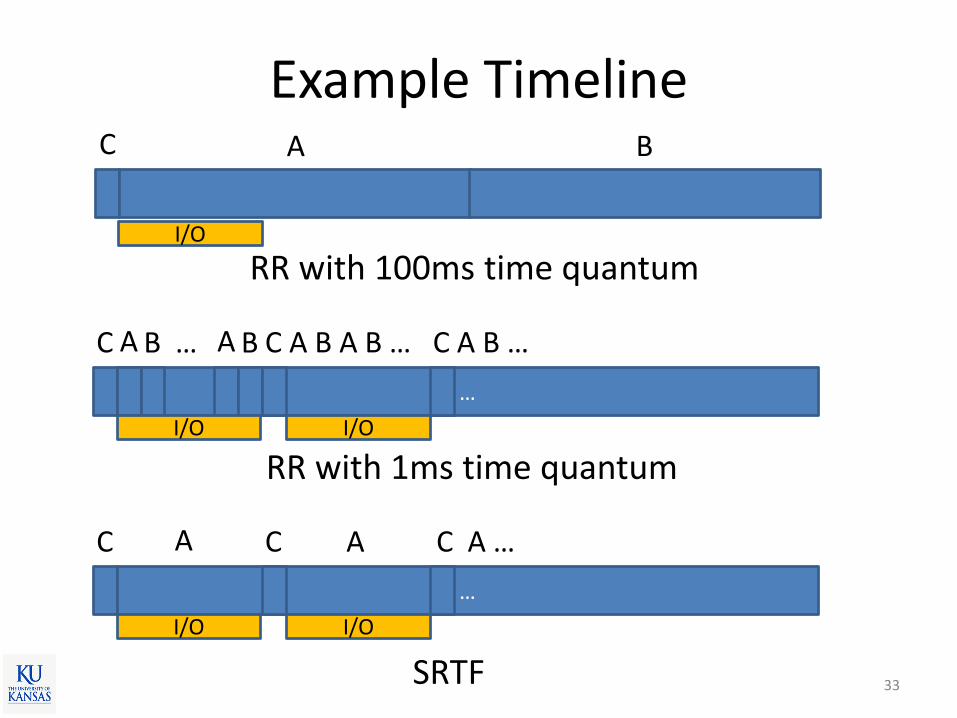
Example Timeline
33
C A B
RR with 100ms time quantum
C
…
A
RR with 1ms time quantum
B … A B
I/O
I/O
C A B A B … C A B …
I/O
C
…
SRTF
A
I/O
C A C A …
I/O

Summary
• First-Come, First-Served (FCFS)– Run to completion in order of arrival
– Pros: simple, low overhead, good for batch jobs
– Cons: short jobs can stuck behind the long ones
• Round-Robin (RR)– FCFS with preemption. Cycle after a fixed time quantum
– Pros: better interactivity (low average scheduling latency)
– Cons: performance is dependent on the quantum size
• Shortest Job First (SJF)/ Shorted Remaining Time First (SRTF)– Shorted job (or shortest remaining job) first
– Pros: optimal average waiting time
– Cons: you need to know the future, long jobs can be starved by short jobs
34
Recommended


![ACCESS CONTROL SYSTEM - TECNOSeguro · SOYAL ACCESS CONTROL SYSTEM ® AR-821EF / AR-821EV V100126 DO MT or P1 P2 P3 P4 P1 P2 P3 P4 P1 P2 P3 P4 1 2 A. B. Contents AR-821EF [Fingerprint]](https://img.dokumen.tips/doc/110x75/5ec109a28b6964497d2229e9/access-control-system-tecnoseguro-soyal-access-control-system-ar-821ef-ar-821ev.jpg)