Lecture 19Fitting CAR and SAR Models
Colin Rundel03/29/2017
1

Fitting areal models
2

CAR vs SAR
• Simultaneous Autogressve (SAR)
y(si) = ϕn∑j=1
Wij y(sj) + ϵ
y ∼ N (0, σ2 ((I − ϕW)−1)((I − ϕW)−1)t)
• Conditional Autoregressive (CAR)
y(si)|y−si ∼ N
ϕn∑j=1
Wij y(sj), σ2
y ∼ N (0, σ2 (I − ϕW)−1)
3

Some specific generalizations
Generally speaking we will want to work with a scaled / normalized versionof the weight matrix,
Wij
Wi·
When W is an adjacency matrix we can express this as
D−1W
where D = diag(mi) and mi = |N(si)|.
We can also allow σ2 to vary between locations, we can define this asDτ = diag(1/σ2
i ) and most often we use
Dτ = diag(
1σ2/|N(si)|
)= D/σ2
where D is as defined above.
4

Revised CAR Model
• Conditional Model
y(si)|y−si ∼ N
Xi·β + ϕn∑j=1
Wij
Dii
(y(sj) − Xj·β
), σ2D−1
ii
• Joint Model
y ∼ N (Xβ, ΣCAR)
ΣCAR = (Dσ (I − ϕD−1W))−1
= (1/σ2D (I − ϕD−1W))−1
= (1/σ2(D − ϕW))−1
= σ2(D − ϕW)−1 5

Revised SAR Model
• Formula Model
y(si) = Xi·β + ϕn∑j=1
D−1jj Wij
(y(sj) − Xj·β
)+ ϵi
• Joint Model
y = Xβ + ϕD−1W(y − Xβ
)+ ϵ(
y − Xβ)= ϕD−1W
(y − Xβ
)+ ϵ(
y − Xβ)(I − ϕD−1W)−1 = ϵ
y = Xβ + (I − ϕD−1W)−1ϵ
y ∼ N(Xβ, (I − ϕD−1W)−1σ2D−1((I − ϕD−1W)−1)t)
6

Toy CAR Example
s1
s2
s3
W =
0 1 01 0 10 1 0
D =
1 0 00 2 00 0 1
Σ = σ2 (D − ϕW) = σ2
1 −ϕ 0−ϕ 2 −ϕ0 −ϕ 1
−1
7

Toy CAR Example
s1
s2
s3
W =
0 1 01 0 10 1 0
D =
1 0 00 2 00 0 1
Σ = σ2 (D − ϕW) = σ2
1 −ϕ 0−ϕ 2 −ϕ0 −ϕ 1
−1
7

When does Σ exist?
check_sigma = function(phi) {Sigma_inv = matrix(c(1,-phi,0,-phi,2,-phi,0,-phi,1), ncol=3, byrow=TRUE)solve(Sigma_inv)
}
check_sigma(phi=0)## [,1] [,2] [,3]## [1,] 1 0.0 0## [2,] 0 0.5 0## [3,] 0 0.0 1
check_sigma(phi=0.5)## [,1] [,2] [,3]## [1,] 1.1666667 0.3333333 0.1666667## [2,] 0.3333333 0.6666667 0.3333333## [3,] 0.1666667 0.3333333 1.1666667
check_sigma(phi=-0.6)## [,1] [,2] [,3]## [1,] 1.28125 -0.46875 0.28125## [2,] -0.46875 0.78125 -0.46875## [3,] 0.28125 -0.46875 1.28125
8

check_sigma(phi=1)## Error in solve.default(Sigma_inv): Lapack routine dgesv: system is exactly singular: U[3,3] = 0
check_sigma(phi=-1)## Error in solve.default(Sigma_inv): Lapack routine dgesv: system is exactly singular: U[3,3] = 0
check_sigma(phi=1.2)## [,1] [,2] [,3]## [1,] -0.6363636 -1.363636 -1.6363636## [2,] -1.3636364 -1.136364 -1.3636364## [3,] -1.6363636 -1.363636 -0.6363636
check_sigma(phi=-1.2)## [,1] [,2] [,3]## [1,] -0.6363636 1.363636 -1.6363636## [2,] 1.3636364 -1.136364 1.3636364## [3,] -1.6363636 1.363636 -0.6363636
9

Conclusions
Generally speaking just like the AR(1) model for time series we require that|ϕ| < 1 for the CAR model to be proper.
These results for ϕ also apply in the context where σ2i is constant across
locations (i.e. Σ = (σ2 (I − ϕD−1W))−1)
As a side note, the special case where ϕ = 1 is known as an intrinsicautoregressive (IAR) model and they are popular as an improper prior forspatial random effects. An additional sum constraint is necessary foridentifiability (
∑i = 1ny(si) = 0).
10

Example - NC SIDS
34°N
34.5°N
35°N
35.5°N
36°N
36.5°N
84°W 82°W 80°W 78°W 76°W
10000
20000
30000BIR79
34°N
34.5°N
35°N
35.5°N
36°N
36.5°N
84°W 82°W 80°W 78°W 76°W
0
10
20
30
40
50
SID79
11
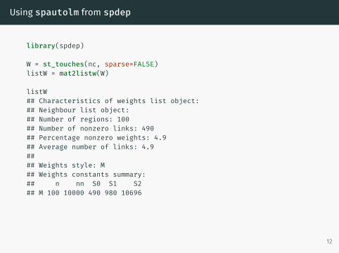
Using spautolm from spdep
library(spdep)
W = st_touches(nc, sparse=FALSE)listW = mat2listw(W)
listW## Characteristics of weights list object:## Neighbour list object:## Number of regions: 100## Number of nonzero links: 490## Percentage nonzero weights: 4.9## Average number of links: 4.9#### Weights style: M## Weights constants summary:## n nn S0 S1 S2## M 100 10000 490 980 10696
12

nc_coords = nc %>% st_centroid() %>% st_coordinates()
plot(st_geometry(nc))plot(listW, nc_coords, add=TRUE, col=”blue”, pch=16)
13

CAR Model
nc_car = spautolm(formula = SID74 ~ BIR74, data = nc,listw = listW, family = ”CAR”)
summary(nc_car)#### Call:## spautolm(formula = SID74 ~ BIR74, data = nc, listw = listW, family = ”CAR”)#### Residuals:## Min 1Q Median 3Q Max## -10.38934 -1.58600 -0.52154 1.14729 13.54059#### Coefficients:## Estimate Std. Error z value Pr(>|z|)## (Intercept) 1.06911902 0.67501301 1.5838 0.1132## BIR74 0.00175249 0.00010107 17.3401 <2e-16#### Lambda: 0.13222 LR test value: 8.8654 p-value: 0.0029062## Numerical Hessian standard error of lambda: 0.030094#### Log likelihood: -275.7655## ML residual variance (sigma squared): 13.695, (sigma: 3.7007)## Number of observations: 100## Number of parameters estimated: 4## AIC: 559.53
14
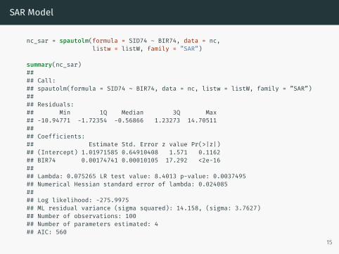
SAR Model
nc_sar = spautolm(formula = SID74 ~ BIR74, data = nc,listw = listW, family = ”SAR”)
summary(nc_sar)#### Call:## spautolm(formula = SID74 ~ BIR74, data = nc, listw = listW, family = ”SAR”)#### Residuals:## Min 1Q Median 3Q Max## -10.94771 -1.72354 -0.56866 1.23273 14.70511#### Coefficients:## Estimate Std. Error z value Pr(>|z|)## (Intercept) 1.01971585 0.64910408 1.571 0.1162## BIR74 0.00174741 0.00010105 17.292 <2e-16#### Lambda: 0.075265 LR test value: 8.4013 p-value: 0.0037495## Numerical Hessian standard error of lambda: 0.024085#### Log likelihood: -275.9975## ML residual variance (sigma squared): 14.158, (sigma: 3.7627)## Number of observations: 100## Number of parameters estimated: 4## AIC: 560
15

Residuals
34°N34.5°N
35°N35.5°N
36°N36.5°N
84°W 82°W 80°W 78°W 76°W0
10
20
30
car_pred
34°N34.5°N
35°N35.5°N
36°N36.5°N
84°W 82°W 80°W 78°W 76°W10
20
30
sar_pred
34°N34.5°N
35°N35.5°N
36°N36.5°N
84°W 82°W 80°W 78°W 76°W−10
−5
0
5
10
car_resid
34°N34.5°N
35°N35.5°N
36°N36.5°N
84°W 82°W 80°W 78°W 76°W−10
−5
0
5
10
car_resid
16

I agree …
17

Why?
Histogram of nc$SID74
nc$SID74
Fre
quen
cy
0 10 20 30 40
010
2030
4050
60
−2 −1 0 1 2
−10
−5
05
10
CAR Residuals
Theoretical Quantiles
Sam
ple
Qua
ntile
s
−10 −5 0 5 10
−10
−5
05
1015
CAR vs SAR Residuals
nc$car_resid
nc$s
ar_r
esid
18

Jags CAR Model
## model{## y ~ dmnorm(beta0 + beta1*x, tau * (D - phi*W))## y_pred ~ dmnorm(beta0 + beta1*x, tau * (D - phi*W))#### beta0 ~ dnorm(0, 1/100)## beta1 ~ dnorm(0, 1/100)#### tau <- 1 / sigma2## sigma2 ~ dnorm(0, 1/100) T(0,)## phi ~ dunif(-0.99, 0.99)## }
y = nc$SID74x = nc$BIR74
W = W * 1LD = diag(rowSums(W))
Why don’t we use the conditional definition for the y’s?
19

Model Results
16000 18000 20000 22000 24000
−2
26
Iterations
Trace of beta0
−2 0 2 4 6 8 10
0.0
0.2
0.4
Density of beta0
N = 1000 Bandwidth = 0.1893
16000 18000 20000 22000 24000
0.00
130.
0017
Iterations
Trace of beta1
0.0014 0.0016 0.0018 0.0020
020
00
Density of beta1
N = 1000 Bandwidth = 2.279e−05
20

16000 18000 20000 22000 24000
0.2
0.6
1.0
Iterations
Trace of phi
0.2 0.4 0.6 0.8 1.0
0.0
1.0
2.0
Density of phi
N = 1000 Bandwidth = 0.03673
16000 18000 20000 22000 24000
4050
60
Iterations
Trace of sigma2
40 50 60 700.
000.
040.
08
Density of sigma2
N = 1000 Bandwidth = 1.188
21

Predictions
nc$jags_pred = y_pred$post_meannc$jags_resid = nc$SID74 - y_pred$post_mean
sqrt(mean(nc$jags_resid^2))## [1] 3.987985sqrt(mean(nc$car_resid^2))## [1] 3.72107sqrt(mean(nc$sar_resid^2))## [1] 3.762664
34°N34.5°N
35°N35.5°N
36°N36.5°N
84°W 82°W 80°W 78°W 76°W10
20
30
jags_pred
34°N34.5°N
35°N35.5°N
36°N36.5°N
84°W 82°W 80°W 78°W 76°W−10
−5
0
5
10
15jags_resid
22

0
10
20
30
0 10 20 30 40
car_pred
jags
_pre
d
23

Brief Aside - SAR Precision Matrix
ΣSAR = (I − ϕD−1 W)−1σ2 D−1 ((I − ϕD−1 W)−1)t
Σ−1SAR =
((I − ϕD−1 W)−1σ2 D−1 (
(I − ϕD−1 W)−1)t)−1
=(((I − ϕD−1 W)−1)t)−1 1
σ2 D (I − ϕD−1 W)
=1
σ2 (I − ϕD−1 W)t D (I − ϕD−1 W)
24
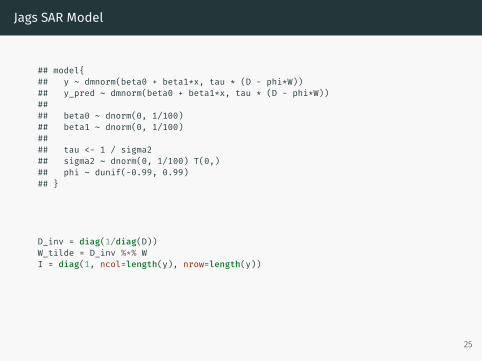
Jags SAR Model
## model{## y ~ dmnorm(beta0 + beta1*x, tau * (D - phi*W))## y_pred ~ dmnorm(beta0 + beta1*x, tau * (D - phi*W))#### beta0 ~ dnorm(0, 1/100)## beta1 ~ dnorm(0, 1/100)#### tau <- 1 / sigma2## sigma2 ~ dnorm(0, 1/100) T(0,)## phi ~ dunif(-0.99, 0.99)## }
D_inv = diag(1/diag(D))W_tilde = D_inv %*% WI = diag(1, ncol=length(y), nrow=length(y))
25

Model Results
26000 28000 30000 32000 34000
−1
13
Iterations
Trace of beta0
−2 −1 0 1 2 3 4
0.0
0.3
0.6
Density of beta0
N = 1000 Bandwidth = 0.1679
26000 28000 30000 32000 34000
0.00
140.
0018
Iterations
Trace of beta1
0.0014 0.0016 0.0018
020
00
Density of beta1
N = 1000 Bandwidth = 2.108e−05
26

26000 28000 30000 32000 34000
0.1
0.4
0.7
Iterations
Trace of phi
0.0 0.2 0.4 0.6 0.8
0.0
1.5
3.0
Density of phi
N = 1000 Bandwidth = 0.02809
26000 28000 30000 32000 34000
4050
60
Iterations
Trace of sigma2
40 45 50 55 60 65 700.
000.
040.
08
Density of sigma2
N = 1000 Bandwidth = 1.109
27

Comparing Model Results
phi sigma2
beta0 beta1
0.25 0.50 0.75 20 30 40 50 60
0 1 2 0.0015 0.0016 0.0017 0.0018
value
model
JAGS CAR
JAGS SAR
spautolm CAR
spautolm SAR
28
Recommended