
Lecture 11: Potential Energy Functions
Dr. Ronald M. Levy
Originally contributed by Lauren Wickstrom (2011)
Statistical Thermodynamics
Statistical ThermodynamicsSpring 2013
Microscopic/Macroscopic Connection
• The connection between microscopic interactions and macroscopic thermodynamic properties is encoded in the potential energy function U(x)
Z =∫ dx e−βU ( x )
• A model of the system starts with the specification of its potential energy function

Statistical ThermodynamicsSpring 2013
Terminology
• Potential Energy – non-kinetic part of the internal energy of a system.
• Molecular Mechanics - Classical mechanics description of the potential energy.
• Function of nuclear positions (electronic motion neglected) – Born-Oppenheimer approximation
• Force field – Parameterized, analytical function of the potential energy
• All-Atom Force Field – Function of the positions of all of the atoms (as opposed to a coarse-grained force field).
Statistical ThermodynamicsSpring 2013
Some Common All-atom force fields for biomolecules
• OPLS (Optimized Potential for Liquid Simulations) – Jorgensen/Friesner
• AMBER (Assisted Model Building with Energy Refinement)* – Kollman/Case
• CHARMM (Chemistry at Harvard Molecular Mechanics)* – Karplus
• GROMOS (GROningen MOlecular Simulation package)* –Berendsen and van Gunsteren
• AMOEBA (Atomic Multipole Optimized Energetics for Biomolecular Applications) Ren & Ponder
• ECEPP (Empirical Conformational Energy Program for Peptides) - Scheraga
*These are force fields as well as simulation packages.

Statistical ThermodynamicsSpring 2013
Born-Oppenheimer formulation
Molecular degrees of freedom: nucleii positions (x) For each configuration of the nucleii we have a series of
electronic states at energies E0, E1, E2, ...
Assume that electrons readjust instantaneously to new positions of the nucleii.
System always remains in ground state at energy
E 0=E 0(x) E
0(x) can in princible be evaluated at
each x by QM methods (Gaussian, etc.) In practice need a simple function that mimics as best as
possible the true E0(x)

Statistical ThermodynamicsSpring 2013
Typical formulation of a Non-polarizable Non-dissociative Force Field:
Energy terms Interactions
Vbond1-2
Vangle1-3
Vtorsions1-4
VLJ,Vcoul.Non-bonded
V r =∑bonds
k ij
2d ij−d ij , 0
2 ∑angles
k ijk
2ijk−ijk , 0
2
∑torsions
V ijkl ,n
2[1cos n ijkl− ijkl] ∑
non−bonded [4 ij ij12
r ij12 −
ij6
r ij6 qi q j
40 r ij ]
Torsion
Bond
Bond Angle
Non-Bonded

Statistical ThermodynamicsSpring 2013
Bond stretching
V bond=De [1−e−a d−d 0 ]2
D e=depth of potential energy mininum
Morse Potential
a=width of potential welld 0=equilibrium bond length
V bond=k2d−d 0
2
Hooke's lawHooke's law
– harmonic approximation – non dissociative– reasonable for small displacements

Statistical ThermodynamicsSpring 2013
Bond stretching parameters
• k obtained from vibrational spectra
• d0 obtained from X-ray
crystallography
• Hard degree of freedom
• Often constrained in MD
If δd = .2 Å for carbonyl
Vbond = 11.4 kcal/mol
Type k (kcal/mol/ Å2) d0(Å)
CA-N 337 1.44
C=O 570 1.22
CAN CO
V bond=k2d−d 0
2

Statistical ThermodynamicsSpring 2013
Angle bending
• Hooke’s Law in anglecoordinates
V angle=k
2−0
2
Type Kθ(kcal/mol/ radian2) θ0(deg)
N-CA-HA 35 109.5
CA-C-O 80 120.4
If δθ= 4° for CA-C-0Vangle = 11.6 kcal/mol
CAC N
O
HA
N

Statistical ThermodynamicsSpring 2013
Torsional terms Black: Vn=4; n=2; γ=180Red: Vn=2; n=3;γ=0
• Barriers of rotation
• Ethane – 9 dihedral angles (H-C-C-H)
Butane – 27 dihedral angles (1 C-C-C-C, 10 H-C-C-C,
16 H-C-C-H)
V n=amplituden=periodicity n= phase
V torsion=∑n
V n
2[1cosn−n]
Fourier expansion

Statistical ThermodynamicsSpring 2013
• 120 degrees periodicity
• Parameters are obtained by fitting to high level QM data
Torsional parameters
Torsion angle Vn
N-CA-CB-HB1 .23
N-CA-CB-HB2 .23
N-CA-CB-HB3 .23
V torsion=V 0V 3
2[1cos 3]

Statistical ThermodynamicsSpring 2013
Improper torsions
• Describe out of plane motion
• This is often important to maintain planar structure.
Examples:
Peptide bond
Benzene
• OPLS – adjusts force constants instead of using improper function
V improper=∑n
k i
2ijkl−0
2
V improper=V 2
2[1cos 2ijkl−]
Statistical ThermodynamicsSpring 2013
Non-bonded interactions: Electrostatic
• Important “directional” interaction energy term
• Charge distribution calculated from QM calculations
• Electrostatic interaction between two molecules:
V mp=∫ dr dr 'mr pr '
∣r−r '∣

Statistical ThermodynamicsSpring 2013
Electrostatics One representation: Multipole Expansion Charge distribution represented in terms of its moments (charges, dipoles, quadrupoles, octupoles)
r q , , Q ,

Statistical ThermodynamicsSpring 2013
Different types of multipole interactions
• Interactions become weaker with higher multipole moments
• Attraction or repulsion -charge and orientation of the dipole
Type of interaction
Distance r Dependence
Charge-charge 1/r
Charge-dipole 1/r2
Dipole/dipole 1/r3
Dipole/induced dipole 1/r6
+ δ+ δ-
Charge Dipole
UNFAVORABLE
- δ+ δ-
Charge Dipole
FAVORABLE

Statistical ThermodynamicsSpring 2013
Example:
Benzene – Benzene interaction
• 144 charge-charge interactions
• First term: quadrupole-quadruple calculation (no monopole, no dipole)
• Only valid when the distance between two molecules is much larger than the internal dimensions.
• Multipolar expansions are computationally expensive

Statistical ThermodynamicsSpring 2013
More common representation: partial charges
• Charge distribution described by delta functions at “charged sites” (usually atomic sites)
Partial charges from:• Fit to experimental liquid properties (OPLS)• ESP charge fitting to reproduce electrostatic potentials of high level QM• X-ray crystallographic electron density
r ≈∑iqir i
V mp≈∑ij
qi q j
∣r i−r j∣
Statistical ThermodynamicsSpring 2013
Polarization
• Charges can induce other charge asymmetries by polarization
• Most common strategy is to employ pre-polarized charge distributions
Example: Dipole of water in vacuum = 1.8 D
Dipole fit to yield liquid properties = 2.2-2.5 D
Sometimes overlooked work for creating polarized charge distribution:
E = electric fieldμ = dipole α=point polarizablity
V self =∫0
iE · d =∫0
i α
· d = i2 /2α

Statistical ThermodynamicsSpring 2013
Explicit treatment of polarization
• Induced dipole
= E
Interactions between permanent charges, between charges and induced dipoles and between induced dipoles
Induced dipoles and electrostatic field solved to self-consistency
Polarization energy V pol=−12∑i
i E 0
= Electric field from permanent chargesE 0
Most commonly used “fixed-charge” force fields to not treat explicit polarization
Statistical ThermodynamicsSpring 2013
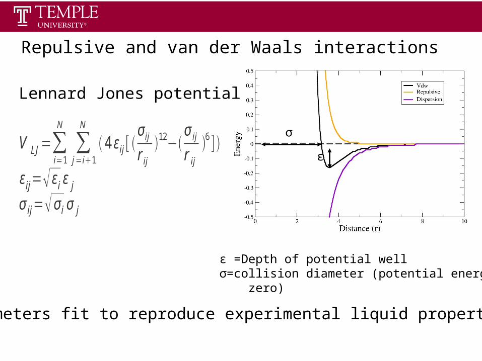
σ
Parameters fit to reproduce experimental liquid properties
σ
ε
ε =Depth of potential wellσ=collision diameter (potential energy = zero)
Repulsive and van der Waals interactions
V LJ=∑i=1
N
∑j=i1
N
4 εij [ σ ij
r ij
12−σ ij
r ij
6 ]
εij= εi ε j
σ ij= σ i σ j
Lennard Jones potential

Statistical ThermodynamicsSpring 2013
1,4 interactions
• Electrostatics + LJ interactions
• 1-2, 1-3 interactions excluded
• 1-4 interactions scaled
• Inclusion in bonded terms of force field
Force field Electrostatics(factor) van der Waals
OPLS .5 .5
AMBER .83 .5
CHARMM 1 1
1-2
1-3
1-4
Statistical ThermodynamicsSpring 2013
Computational timing of different force field terms
• Different parts of the energy scale differently
• Bonded – linear
• Non-bonded interactions – N2
• Requires most computational time
• Cutoffs must be implemented to reduce this cost
Statistical ThermodynamicsSpring 2013
Final thoughts
• Force fields rely on experimental data for parameterization
• Validation is also a key aspect of building these models (experimental observables)
• Time scale and sampling are important aspects are essential for force field evaluation
• One must know the limitations of particular models (force field biases)

Statistical ThermodynamicsSpring 2013
Solvation: Solvent Potential of Mean Force W:Implicit solvent
• Approximate model
• Averages solvation effect (potential mean force)
• High dielectric = solvent; Low dielectric = solute
• Less friction than water (faster transitions)
• Fewer degrees of freedom
ε=80
ε=1
Recommended


