Lecture07 February 12, 2008
Lecture 07: Interpolation
Outline
1) Definitions, Motivation and Applications of Interpolation2) Polynomial Interpolation!
Definition and uniqueness of the interpolating polynomial PNFinding PN
Monomial Basis: Vandermonde matrices and PolyfitLagrange Basis: Newton Basis:?Properties of the Lagrange PolynomialsExamples
3) Error Estimates for Polynomial InterpolationLagrange Remainder FormulaChebyshev points for reducing error (if you can)
4) There's more to life than polynomials...
Interpolation and Interpolants
Definition: Given a discrete set of values yi at locations xi, an interpolant is a (piecewise) continuous function f(x) that passes exactly through the data (i.e. f(xi)=yi).
Comments: lots of methods of interpolation, lots of different functions, works in n-Dimensions.

Lecture07 February 12, 2008
Interpolation and Interpolants
Some Applications:Data filling: Connect the dotsFunction Approximation: Fundamental Component of other algorithms
Rootfinding: Secant method and IQIOptimization: successive parabolic interpolationNumerical integration and differentiationFinite Element Methods!
Polynomial Interpolation (1-D)The Interpolating Polynomial:
Theorem: There is a unique polynomial of degree N, PN(x) that passes exactly through N+1 values y1...yN+1 at distinct positions x1...xN+1 (i.e. PN(xi)=yi)
Example: 2 points
3 points:
Lecture07 February 12, 2008
Polynomial Interpolation (1-D)The Interpolating Polynomial:
Theorem: There is a unique polynomial of degree N, PN(x) that passes exactly through N+1 values y1...yN+1 at distinct positions x1...xN+1 (i.e. PN(xi)=yi)
Proof: Let PN(x)=p1xN + p2xN-1 + ... + pN x +pN+1 such that PN(xi)=yi for i=1,...,N+1 and xi≠xj ∀ i,j
Now assume that there is another degree N polynomial Q that passes through the same points i.e.
QN(x)=q1xN + q2xN-1 + ... + qN x +qN+1 and QN(xi)=yi
Finding the interpolating Polynomial:Monomial Basis
Let PN(x)=p1xN + p2xN-1 + ... + pN x +pN+1 which is a Linear combination of the monomials
1, x, x2, x3, ..., xN with weights p1,p2,...pN+1
Lecture07 February 12, 2008
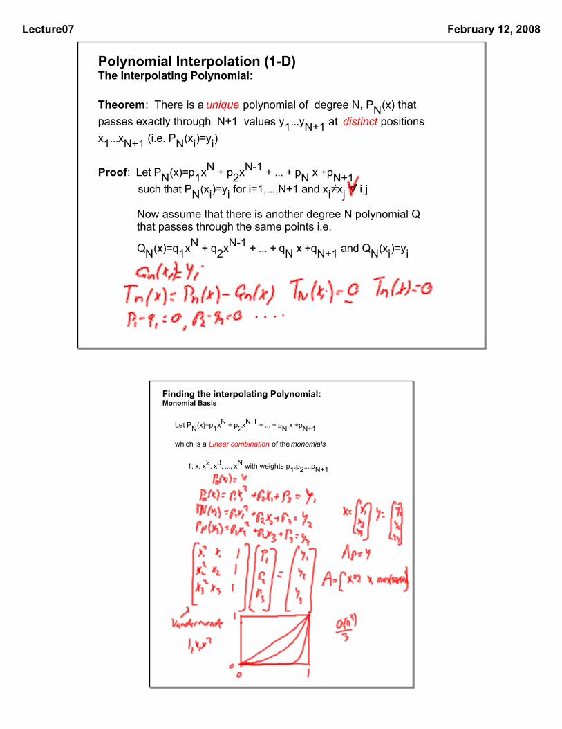
Finding the interpolating Polynomial:Matlab:
Easiest:
Next Easiest:
Break it down:
function A = vander(v)n = length(v);v = v(:);A = ones(n);for j = n-1:-1:1 A(:,j) = v.*A(:,j+1);end
Finding the interpolating Polynomial: A better wayLagrange basis:
define the Lagrange Polynomials of order N as
Examples: for 2 points, N=1 (linear)
3 points: N=2 (quadratic)

Lecture07 February 12, 2008
See Demo FunctionL = seeLagrange(xNodes);

Lecture07 February 12, 2008
Finding the interpolating Polynomial: A better wayLagrange basis:
Fundamental properties of the Lagrange Polynomials
1) Lk(xi) =
2) The interpolating polynomial can be written exactly as
PN(x) =
Polynomial Interpolation using Lagrange:Moler's polyinterp
function y = polyinterp(xNodes,yNodes,x)%POLYINTERP Polynomial interpolation.% y = POLYINTERP(xNodes,yNodes,x) computes y(j) = P(x(j)) where P is the% polynomial of degree d = length(xNodes)-1 with P(xNodes(i)) = yNodes(i). % Use Lagrangian representation.% Evaluate at all elements of u simultaneously.% Modified from Moler: NCM routines n = length(xNodes); % number of interpolating pointsy = zeros(size(x));for k = 1:n w = ones(size(x)); % start calculating Lagrange Weights for j = [1:k-1 k+1:n] % skip over node k w = (x-xNodes(j))./(xNodes(k)-xNodes(j)).*w; end y = y + w*yNodes(k);end

Lecture07 February 12, 2008
Polynomial Interpolation using Lagrange:
Examples: Interpolate sin(pi*x) using 6 equally spaced points on the interval [ -1 1]
xNodes = linspace(_________);yNodes = x = y = polyinterp(xNodes,yNodes,x);
Figure created using Demo Code [ y, error ] = seeInterp(func,x,xNodes)
Polynomial Interpolation using Lagrange:
Examples: Interpolate sin(pi*x) using 6 equally spaced points on the interval [ -1 1]

Lecture07 February 12, 2008
Polynomial Interpolation using Lagrange:
Examples: Interpolate sin(pi*x) using 11 equally spaced points on the interval [ -1 1]
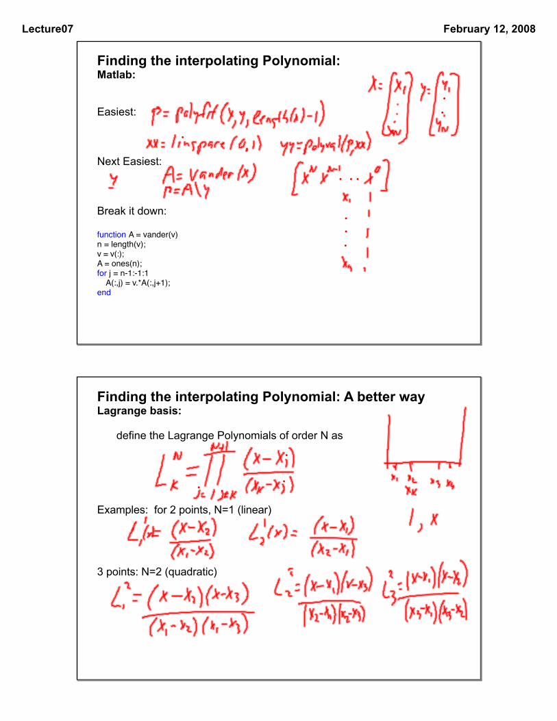
Polynomial Interpolation using Lagrange:
Warning! High Order does not guarantee high accuracy!(only if your function or data is well approximated by a high-order polynomial)
Example #2: Interpolate Runge's Function f(x) = 1/(1+25x2) using 6 points on the interval [ -1 1];
Lecture07 February 12, 2008
Polynomial Interpolation using Lagrange:
Warning! High Order does not guarantee high accuracy!(only if your function or data is well approximated by a high-order polynomial)
Example #2: Interpolate Runge's Function f(x) = 1/(1+25x2) using 11 points on the interval [ -1 1];
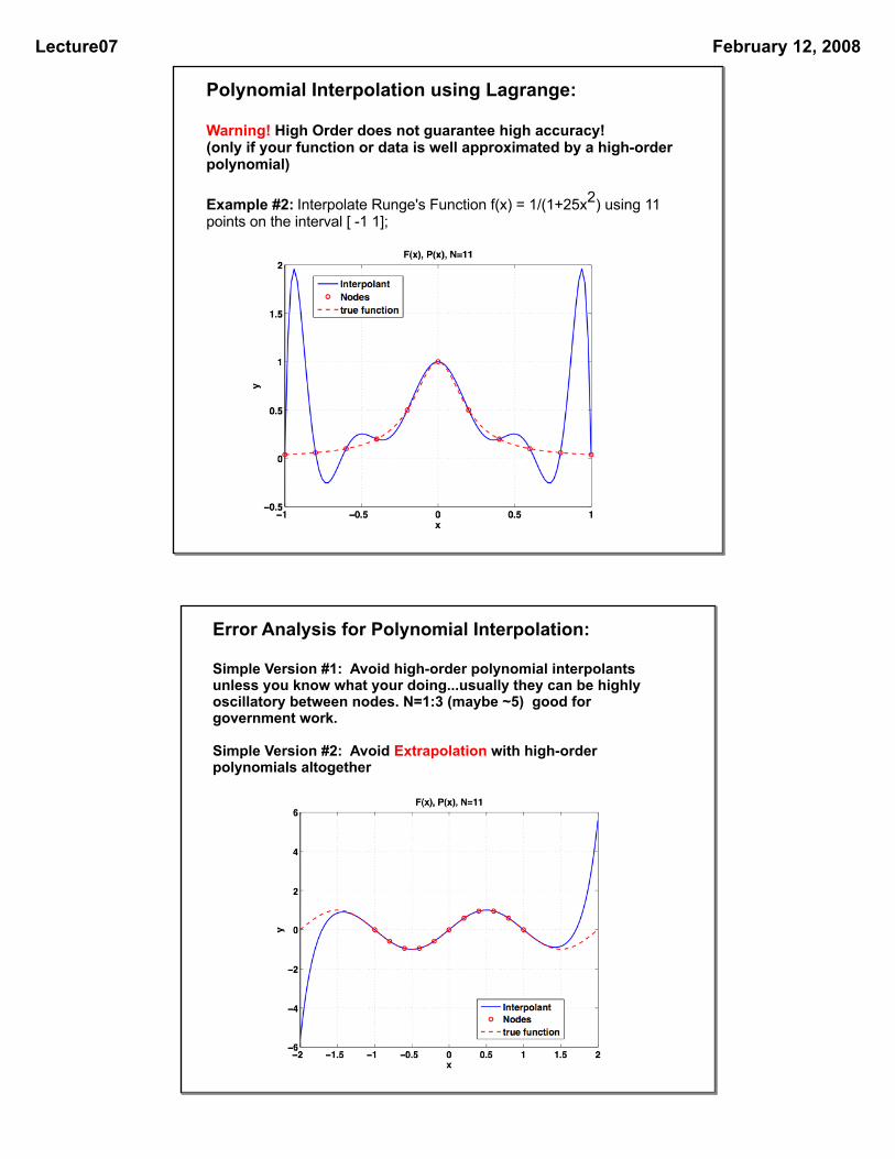
Error Analysis for Polynomial Interpolation:
Simple Version #1: Avoid high-order polynomial interpolants unless you know what your doing...usually they can be highly oscillatory between nodes. N=1:3 (maybe ~5) good for government work.
Simple Version #2: Avoid Extrapolation with high-order polynomials altogether

Lecture07 February 12, 2008
Error Analysis for Polynomial Interpolation:Less Simple version:
Lagrange Remainder Theorem: similar to Taylor's Theorem
Theorem: let f(x) ∈ CN+1[-1,1], then
f(x) = PN(x) + RN(x)
where PN(x) is the interpolating polynomial and
RN(x) = Q(x) f(N+1)(c)/(N+1)! with c ∈ [a,b] and
Q(x) = (x-x1)(x-x2)(x-x3)...(x-xN+1)
Comments:
Q(x) is a N+1 order monic polynomial (leading coefficient = 1)
for Taylor's Theorem Q(x) = __________and the error vanishes identically at x=
for Lagrange: Q(x) vanishes at?
To minimize RN(x) requires minimizing |Q(x)| for x∈[-1,1]. How?
Error Analysis for Polynomial Interpolation:Less Simple version:
The Magic of Chebyshev Polynomials
Definition: The Chebyshev polynomials are another basis for the space of polynomials with important properties
First 4 Chebyshev Polynomials:
T0(x) = 1T1(x) = x
T2(x) = 2x2-1
T3(x) = 4x3-3x
T4(x) = 8x4-8x2+1
Lecture07 February 12, 2008
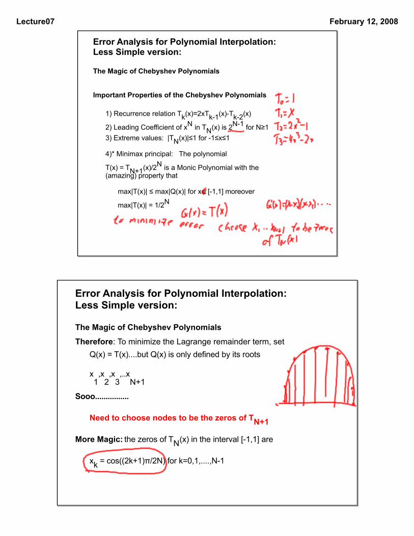
Error Analysis for Polynomial Interpolation:Less Simple version:
The Magic of Chebyshev Polynomials
Important Properties of the Chebyshev Polynomials
1) Recurrence relation Tk(x)=2xTk-1(x)-Tk-2(x)
2) Leading Coefficient of xN in TN(x) is 2N-1 for N≥13) Extreme values: |TN(x)|≤1 for -1≤x≤1
4)* Minimax principal: The polynomial
T(x) = TN+1(x)/2N is a Monic Polynomial with the (amazing) property that
max|T(x)| ≤ max|Q(x)| for x ∈ [-1,1] moreover
max|T(x)| = 1/2N
Error Analysis for Polynomial Interpolation:Less Simple version:
The Magic of Chebyshev Polynomials
Therefore: To minimize the Lagrange remainder term, set Q(x) = T(x)....but Q(x) is only defined by its roots
x1
,x2
,x3
,..xN+1
Sooo................
Need to choose nodes to be the zeros of TN+1
More Magic: the zeros of TN(x) in the interval [-1,1] are
xk = cos((2k+1)π/2N) for k=0,1,....,N-1

Lecture07 February 12, 2008
Comparison of Interpolation with equally spaced points vs Chebyshev points
N = 11;x=linspace(-1,1);xNodes = chebyshevZeros(N-1);f = @(x) 1./(1+25*x.^2)[ y, error ] = seeInterp(f,x,xNodes,'showerror');
Comparison of Interpolation with equally spaced points vs Chebyshev points
N = 11;x=linspace(-1,1);xNodes = chebyshevZeros(N-1);f = @(x) 1./(1+25*x.^2)[ y, error ] = seeInterp(f,x,xNodes,'showerror');

Lecture07 February 12, 2008
Polynomial Interpolation:Some final comments:
0) Interpolation is a fundamental tool in the numerical quiver
1) The interpolating polynomial is only guaranteed to match the data at N points
2) High order polynomials can be wildly innacurate between nodes
3) High order is not High Accuracy!
4) There are a lot more interpolants than full polynomials....Onwards to piecewise-polynomial interpolation
Recommended