Leak Localization in
open water Channels
Nadia Bedjaoui
Workshop on irrigation channels and related problems
N.Bedjaoui, E.Weyer and G. Bastin

2
Outline
• Problem statement
• Objective of this work
• Leak localization methods
• Application
• Conclusion

3
Outline
• Problem statement
• Objective of this work
• Leak localization methods
• Application
• Conclusion

4
• Irrigation channel = supply water to users for irrigation purposes
• Supply done with less water losses possible
• Manual control large water losses
• Automatic control minimizes these losses
• Additional water losses due to the presence of leaks
• Leak =wasted water left definitively from
the channel
Problem statement•Outline Problem statement Objective Methods Application

5
•Outline Problem statement Objective Methods Application
Types of leaks in irrigation channelsProblem statement
• Failures in the civil engineering: Affect the walls of the channel

6
• Failures in the civil engineering:Affect an escape gate
•Outline Problem statement Objective Methods Application
Types of leaks in irrigation channelsProblem statement

7
Types of leaks in irrigation channels
• Unpredicted offtakes Affect the farmer offtakes
•Outline Problem statement Objective Methods Application
Problem statement

8
• Important to
– Detect the presence of the leak– Estimate the size of the leak– Localize the position of the leak
•Outline Problem statement Objective Methods Application
Problem statement

9
Leak Detection + Estimation(E. Weyer& G. Bastin 2008)– Based on mass-balance model
– Idea :Do the measurements check the model?
– CUSUM algorithm: quick detection+ no faulse alarm
– Impossible leak localization
( 1)k
g z k
))()(()()1(
)1( 2/32/3 khcrkhct
kykykz outin
wzw
zw
0
00
Problem statement•Outline Problem statement Objective Methods Application
10
Outline
• Problem statement
• Objective of this work
• Leak localization methods
• Application
• Conclusion

11
Objective of this work
• Interest: leak localization
– Leak is already detected and estimated by CUSUM algorithm (Weyer & Bastin 2008)
• Investigatation of two methods
– Model used: Saint Venant model as Hyperbolic Partial Differential Equations PDE
– Method (1) bank of Nonlinear Saint-Venant models– Method (2) bank of Nonlinear Observers
•Outline Problem statement Objective Methods Application

12
Outline
• Problem statement• Objective of this work
• Leak localization methods
– Method (1) using a bank of pure models• Modelling: Saint Venant is hyperbolic PDE
– Method (2) using a bank on observers• Observer objective• Observer structure• Observer Design
• Application
• Conclusion

13
Method (1): Modelling
•OutlineProblem statementObjective Methods (1)ApplicationConclusion
x=Lx=0
Pool
Upstream Gate
DownstreamGate
PL(t)
Y(t,L)
Leak
Q(t,0)
P0(t)
Q(t,L)
Y(t,0)
w
x
L
xl

14
Method (1): Modelling• Saint Venant Equations
•
• Boundary conditions (x=0 & x=L)(=Gate equations)
• Overshot gate
• Offtake
),()()(),()),(
),((),(
),(),(),(2
xtwA
QkSSgAAYxtgA
xtA
xtQxtQ
xtwxtQxtA
wfxxt
xt
0,1,3/42
22
wkRA
QnS wf
pyhchQ ,2/3
otherwise
xxforwxxwxtw ll 0)(),(
•OutlineProblem statementObjective Methods (1)ApplicationConclusion

15
Method (1):Modelling
Two coupled quasi-linear Hyperbolic PDE
• subcritical flow
( , ) ( , , )t x
A AF A Q f A Q w
Q Q
A
Q
A
QYgA
QAFA
210
),(2
2
wA
QkSSgA
wQAfwf
1
)(
0),,(
0),(
0),(
YgAA
QQA
YgAA
QQA
A
A
•OutlineProblem statementObjective Methods (1)ApplicationConclusion

16
• Initial Conditions (in t=0)
• Boundary Conditions (in x=0 & x=L)
),,(),( wQAfQ
AQAF
Q
Axt
),0()(0 xAxA ),0()(0 xQxQ
)0,(tQ ),( LtQ
•OutlineProblem statementObjective Methods (1)ApplicationConclusion
Method (1):Modelling

17
Method (2):Observer
Method (2): using a bank of Observers
Objective of the observer:
• From any Initial Conditions (t=0)
• Using the only measurements Y(t,0) & Y(t,L)
• The estimation error converges to zero
•OutlineProblem statementObjective Methods (2)ApplicationConclusion
0 0 0 0ˆ ˆ,A A Q Q

18
Method (2): using a bank of Observers
• Observer structure
• Boundary conditions
ˆ ˆˆ ˆ ˆ ˆ ˆ( , ) ( , , )
ˆ ˆt x
A AF A Q f A Q w
Q Q
•OutlineProblem statementObjective Methods (2)ApplicationConclusion
)0,(ˆ tQ ),(ˆ LtQ
Method (2):Observer

19
Method (2): using a bank of Observers• Observer design
1) Linearized model
2) Formulating the estimation problem as a control problem
3) Using the results on boundary control to determine the boundary conditions of the observer that achieves good estimation
•OutlineProblem statementObjective Methods (2)ApplicationConclusion
Method (2):Observer
20
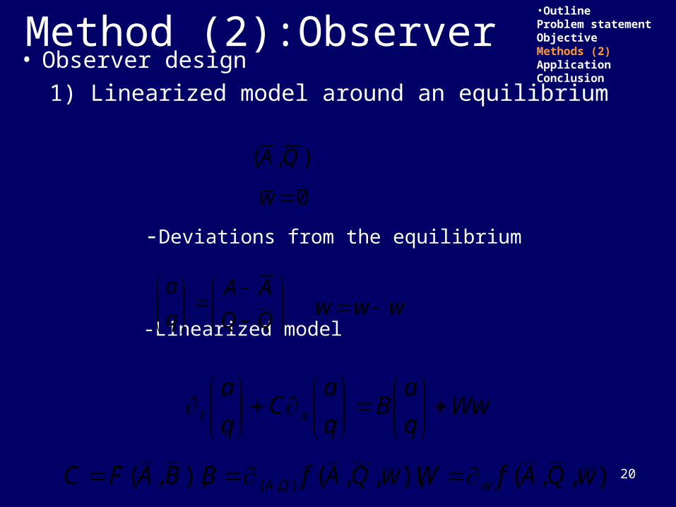
• Observer design
1) Linearized model around an equilibrium
-Deviations from the equilibrium
-Linearized model
•OutlineProblem statementObjective Methods (2)ApplicationConclusion
AA
q
a
0w
Wwq
aB
q
aC
q
axt
),,(),,,(),,( ),( wQAfWwQAfBBAFC wQA
www
Method (2):Observer
),( QA

21
• Observer design
1) Linearized observer around an equilibrium
-Deviations from the equilibrium
-Linearized observer
Estimation error
•OutlineProblem statementObjective Methods (2)ApplicationConclusion
AA
q
aˆ
ˆ
ˆ
ˆ0w
wWq
aB
q
aC
q
axt ˆ
ˆ
ˆ
ˆ
ˆ
ˆ
ˆ
www ˆˆ
AA
aa
e
e
q
a
ˆ
ˆ
ˆ
ˆ
Method (2):Observer
),( QA

22
2) Formulating the estimation problem as a control problem
-Control objective: regulate the deviations to 0 using boundary inputs
-Estimation problem: regulate the estimation error to 0 using the boundary output errors
•OutlineProblem statementObjective Methods (2)ApplicationConclusion
0
0
0
0
AA
q
a
),(
)0,(
),(
)0,(
Lt
t
Ltq
tq
0
0
0
0
ˆ
âa
e
e
q
a
),(
)0,(
),(
)0,(
Lte
te
Lte
te
a
a
Method (2):Observer

23
Summary on boundary control of Saint Venant equations
0( ,0) ( ,0)
( , ) ( , )L
t k t
t L k t L
( ) 0t xx
( ) ( ) ( )t xx B x W x w
-Linear case + non-homogenous terms
-Linear case +non-homogenous terms [ Bastin et al 2008]
small enough for Saint Venant Subcritical flow
B
( , ) ( , , )t x h w
-Quasi-linear case +non-homogenous terms [ Prieur et al 2008]
small enough & sufficiently small'(0) 0, (0)h h
B
w
10 Lkk( , ) 0
( , ) 0t
t
t x
t x

24
observer design based on characteristic method
0 0 0 0 0ˆ ˆ ˆ ˆ( , , ), ( , , )x x x x xL L xL xL xLQ f Q A A Q f Q A A
0 1Lk k
( , ) 0
( , ) 0t
t
e t x
e t x
wxt Weeq
eaB
eq
eaC
eq
ea
weext eW
e
eB
e
e
e
e

25
Method (2): using a bank of Observers
• Initial Conditions (t=0)
• Boundary Conditions (x=0 & x=L)
ˆ ˆˆ ˆ ˆ ˆ ˆ( , ) ( , , )
ˆ ˆt x
A AF A Q f A Q w
Q Q
0 0 0 0ˆ ˆ,A A Q Q
)))0,(ˆ())0,(((1
1
)0,(
)0,(
)0,(ˆ)0,(ˆ 0 tAtA
k
k
tA
tQ
tA
tQ
L
))),(ˆ()),(((1
1
),(
),(
),(ˆ),(ˆ
LtALtAk
k
LtA
LtQ
LtA
LtQ
L
L
,10 LkkA
YgA
AA
•OutlineProblem statementObjective Methods (2)ApplicationConclusion
Method (2):Observer
)))0,(())0,((( tAtAA
Q
A
Q )))0,(())0,((( tAtAA
Q
A
Q

26
Localization scheme
1,{ :min ( )}l j j j
j Nx x J x
1,ˆ ˆ{ :min ( )}l j j j
j Nx x J x
• Method 1
• Method 2
NjxkYkYxLkYLkYxJjT
Tkjjjjj ,1,)),0,()0,(()),,(),(()(
0
22
NjxkYkYxLkYLkYxJjT
Tkjjjjj ,1,))ˆ,0,(ˆ)0,(())ˆ,,(ˆ),(()ˆ(
0
22

27
Outline• Introduction
– Problem statement– Objective of this work
• Leak localization methods
– Method based on models
– Method based on observers
• Application of the 2 methods
– Description of the system of application
– Results and observations with
• Simulated data
• Real data
• Conclusion

28
Application of the 2 methods
• Description of the system of application
Gate 6Gate 5Gate 4Gate 3Gate 2Gate 1
Topview of Coly 6
Farm Farm
L=943m, delay=5mn,
Silde slope=2
Bottom width=1.80m
Gate width=1.91m

29
• Scenario
Pool 5
Gate 4Gate 5
pxL
yxL
Offtake
qx0
px0
qxL
yx0
dxL
Section=35

30
• Scenario
Application on simulated data
Pool 5
Gate 4Gate 5
pxL
yxL
Offtake
qx0
px0
qxL
yx0
dxL
Section=35

310 50 100 150 200 250 300 350 400
-0.2
0
0.2
0.4
0.6
0.8
time [min]
upst
ream
esi
mat
ion
erro
r [m
]
Error estimation for k0 =-0.1and different observer gains
0 50 100 150 200 250 300 350 400-0.2
0
0.2
0.4
0.6
0.8
time [min]
dow
nstre
am e
stim
atio
n er
ror [
m]
Error estimation for k0 =-0.1 and different observer gains
kL=-0.5
kL=-0.1
kL=0
kL=-0.5
kL=-0.1
kL=0
Observer convergence: using different gains

32
Observer convergence from different initial conditions

33
Outline• Introduction
– Problem statement– Objective of this work
• Leak localization methods
– Method based on models
– Method based on observers
• Application of the 2 methods
– Description of the system of application
– Results and observations with
• Simulated data
• Real data
• Conclusion

34
Localization scheme (method 1)

35
Localization scheme (method 2)

36
Results on simulated data
H1H2

37
Localization results on simulated data
0 5 10 15 20 25 30 35 40 45 500
1
x 10-4
sections
Cost fu
nction
model
Observer

38
0 10 20 30 40 500.02
0.03
0.04
0.05
0.06
0.07
0.08
section
Cost fu
nction
Subject to a variation of 50% of n

39
• Scenario
Application on real data
Pool 5
Gate 4Gate 5
pxL
yxL
Offtake
qx0
px0
qxL
yx0
dxL

40
Outline• Introduction
– Problem statement– Objective of this work
• Leak localization methods
– Method based on models
– Method based on observers
• Application of the 2 methods
– Description of the system of application
– Results and observations with
• Simulated data
• Real data
• Conclusion

41
Results on Real data

42
Localization scheme
1,{ :min ( )}l j j j
j Nx x J x
1,ˆ ˆ{ :min ( )}l j j j
j Nx x J x
• Method 1
• Method 2
NjxkYkYxLkYLkYxJjT
Tkjjjjj ,1,)),0,()0,(()),,(),(()(
0
22
NjxkYkYxLkYLkYxJjT
Tkjjjjj ,1,))ˆ,0,(ˆ)0,(())ˆ,,(ˆ),(()ˆ(
0
22

43
Results on simulated data

44
Conclusion Objective: Leak localizationInvestigate two methods for leak localizationMethod (1) based on pure modelsMethod (2) based on observers
Design of observer: - Characteristic method
- The estimation problem is written as boundary control problem for the linearized system
-Convergence of the observer can be fixed by the gains
45
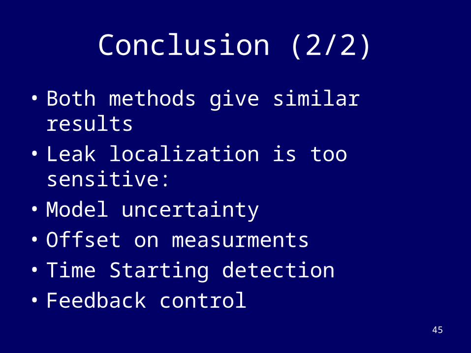
Conclusion (2/2)
• Both methods give similar results
• Leak localization is too sensitive:
• Model uncertainty
• Offset on measurments
• Time Starting detection
• Feedback control
46
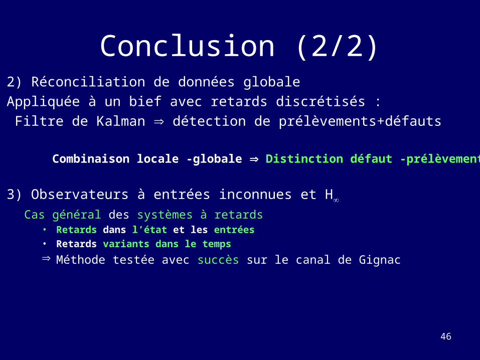
2) Réconciliation de données globale
Appliquée à un bief avec retards discrétisés :
Filtre de Kalman détection de prélèvements+défauts
Combinaison locale -globale Distinction défaut -prélèvement
3) Observateurs à entrées inconnues et H
Cas général des systèmes à retards• Retards dans l’état et les entrées • Retards variants dans le temps
Méthode testée avec succès sur le canal de Gignac
Conclusion (2/2)
Recommended
![JOINT DECLARATION OF JUDGES BEDJAOUI ... DECLARATION OF JUDGES BEDJAOUI, GUILLAUME AND RANJEVA [Translation] Article 31, paragraph 5, of the Statute - United Kingdom and United States](https://img.dokumen.tips/doc/110x75/5ac920a27f8b9a7d548cee3d/joint-declaration-of-judges-bedjaoui-declaration-of-judges-bedjaoui-guillaume.jpg)