
UNIVERSITY OF CONCORDIA
FINAL PROJECT
ELEC6141 - WIRELESSCOMMUNICATIONS
Simulation of A Communications System UsingMatlab
Author:Le Thanh TAN
ID: 6389953INRS-EMT
Instructor:Dr. Yousef R. SHAYAN
University of Concordia
June 16, 2011

1
CONTENTS
I Introduction 1
II System Models and Theoretical Analysis 2II-A The communications system over an AWGN channel . . . . . . . .. . . . . . . . . 2II-B BCH coding scheme . . . . . . . . . . . . . . . . . . . . . . . . . . . . . . . . . .. 3II-C A slow fading channel - Rayleigh model . . . . . . . . . . . . . . . .. . . . . . . 5II-D An interleaving scheme . . . . . . . . . . . . . . . . . . . . . . . . . . .. . . . . . 7
III Numerical Results 8
IV Conclusion 11
Appendix A: Code for a AWGN channel 11
Appendix B: Code for a AWGN channel and a BCH coding 13
Appendix C: Code for a Rayleigh channel 17
Appendix D: Code for a Rayleigh channel and a BCH coding 18
Appendix E: Code for a Rayleigh channel, a BCH coding and an interleaving scheme 20
References 22
I. I NTRODUCTION
In a communications system, the channel is affected by an additive white Gaussian noise (AWGN)and a fading due to a distance between a transmitter and a receiver. Especially, there are many kinds ofchannel fadings. Depending on the moving speeds of transmitters or receivers, a fading type can be a slowfading or a fast fading (i.e., the product of 0.1 and coherence time than smaller or larger than the symbolperiod of signal are corresponding to fast and slow fadings). Moreover, a channel can be referred as aselective fading or a flat fading corresponding to the product of 0.1 and coherence bandwidth than smalleror larger than the bandwidth of signal. These above effects can suffer received signals at a destination.Hence the performance of received signals in term of bit-error-rate (BER) is much degraded.
In order to overcome these issues, communications systems would be carefully designed. In detail,application systems operating over the AWGN channels would use coding schemes to combat an additivewhite noise. However, if environment is affected by fading,coding techniques only solve a fast fading.It implies that, coding schemes degrade received signals when they go through slow fading channels. Inthis case, an interleaving technique would be added to a communications system. In order to overcomethe fading channels, besides, using an interleaver as above, we can exploit the diversity of multi-path. Itimplies that the effects of fading can be combated by transmitting the original signals over multiple paths(experiencing independent fading) and then combining all received signals at the receiver. There are manykinds of diversities to mitigate this issue, such as diversity in time, frequency, and space. Correspondingly,a lot of state-of-art methods are given, viz. diversity receiving and transmitting, OFDM, space-time blockcodes, MIMO, Cooperation and etc.
In summary, the main scope of this report is modeling a communications system. First, I create abasic communications system, where it includes the modulation/demodulation using a QPSK modulation,a channel type is an AWGN channel. Secondly, a coder/decoder scheme is added to a transmitter/receiver toimprove received signals. Thirdly, the fading channel is considered when a receiver/transmitter is moving.It means that the slow fading is mentioned. The performance is shown to prove that the received signal

2
is degraded whether a coding scheme is used or not. Finally, an interleaver/deinterleaver is used to solvethis problem.
Besides, the performance in terms of BER is used to verify a validity of these above techniques in acommunications system.
II. SYSTEM MODELS AND THEORETICAL ANALYSIS
A. The communications system over an AWGN channel
The practical communications systems can be modeled by two following cases such as passband andbaseband models corresponding to Figs. 1 and 2. It is referred that both models are equivalent [2], hencefrom now, the baseband model is analyzed. Let’s summarize the operation of this model. First, an originaldata streamsk(t) = s0, s1, s2, s3, . . . is an input of a QPSK modulation, where bipolar pulses are presentedfor bit sequences. A mapping scheme divides a data stream to an in-phase stream,dI (t), and a quadraturestream,dQ (t), given as
sI (t) = s0, s2, s4, . . . (even bits) , (1)
sQ (t) = s1, s3, s5, . . . (odd bits) . (2)
In Fig. 1, an orthogonal realization of a QPSK waveform is presented as
sTrans (t) =1
√
(2)sI (t) cos (2πf0t)−
1√
(2)sQ (t) sin (2πf0t) , (3)
while an output symbol in Fig. 2 is given as
sSymb = sI (t) + jsQ (t) . (4)
QPSK demodulation
Mapping +
I
jQ
Input
data
stream+
AWGN
Detection
Output
data
stream
QPSK modulation
+
+
cos 2 cf t
sin 2 cf t !
LPF+
cos 2 cf t
+
sin 2 cf t !
LPF
I
Q
Fig. 1. The passband communications model.
The mapping figure is shown in Fig. 3, whered = 1, Eb = 1, henceEs =1
4(4 ∗ 2d2) = 2Eb. We also
note that a modulation and demodulation using the common function presented in Table IIn this subsection, an AWGN channel is considered as Fig. 4. The received signal is
r = s+ n, (5)
wheres andn are the transmitted signal and Gaussian noise, respectively. It is shown in Appendix A thatn is zero mean Gaussian variable with variance ofN0
2for each I and Q components. Theoretical BER of
QPSK modulation is given as [2]
PAWGNb = Q
(
√
2Eb
N0
)
, (6)
whereEb/N0 is signal-to-noise ratio, SNR. Due to AWGN, received signals are lost. Hence a codingscheme is added in order to correct the error at the receiver.

3
QPSK demodulation
Mapping +
I
jQ
Input
data
stream+
AWGN
Detection
Output
data
stream
QPSK modulation
Fig. 2. The baseband communications model.
TABLE ITHE COMMON FUNCTION USED FOR MODULATION/DEMODULATION
x y I Q
0 0 d d1 0 -d d1 1 -d -d0 1 d -d
Fig. 3. The mapping of a QPSK modulation.
B. BCH coding scheme
(15,11,1) BCH coding scheme (i.e.,n = 15, k = 11) is mentioned in this report. In Fig. 5, BCH coderis added before modulator and BCH decoder is after demodulator. The relation between the bit rate andthe symbol rate when using BCH coding scheme is given as
Rc =n
kRb =
15
11Rb, (7)
while
Rs =Rc
logM2
=Rc
2. (8)

4
QPSK demodulation
Mapping +
I
jQ
Input
data
stream+
AWGN
Detection
Output
data
stream
QPSK modulation
Comparison to find BER
Fig. 4. The communications model over a AWGN channel.
Hence,
Rs =15
22Rb. (9)
The new signal-to-noise ratio isEc
N0
= kEb
nN0
. Hence, theoretical BER is calculated as
PBCHb =
1
n
n∑
j=t+1
j
(
n
j
)
Pjc (1− Pc)
n−j, (10)
wherePc = Q(√
2Ec
N0
)
, t = 1.
QPSK demodulation
Mapping +
I
jQ
Input
data
stream+
AWGN
Detection
Output
data
stream
QPSK modulation
Comparison to find BER
Coder Decoder
Fig. 5. The communications model using a coding scheme over a AWGN channel.
In the followings, an implementation of coding scheme is presented.

5
First, the coder is shown, where the generator matrix of (15,11,1) BCH coding scheme is generated as
G =
111110000000000
011101000000000
101100100000000
110100010000000
111000001000000
001100000100000
010100000010000
011000000001000
101000000000100
100100000000010
110000000000001
, (11)
whereG =
[
P...Ik
]
, P is the parity matrix,Ik is the eye matrix. It is also noted that the creation ofG is
illustrated in Appendix B. I omit how to create G due to the limited pages.Secondly, decoder is briefly shown. The syndrome can be received as
S = rHT , (12)
whereH =
[
In−k
...PT
]
which is calculated fromGHT = 0 (note that the creation ofH is shown in
Appendix B), r is the received signal,H is the parity check matrix. Then syndrome table is created,where it includes zero, one and two error patterns (i.e.,t = 1). Besides, the syndrome table has 16rows and2n−k = 16 syndromes. Based on the syndrome table, each received codeword is referred to thecorresponding error pattern on the table. Hence, the received signal can be corrected.
C. A slow fading channel - Rayleigh model
In Global System for Mobile Communications (GSM), the most concerned issue is a fading effect.There are many kinds of fading such as selective fading vs flatfading and slow fading vs fast fadingwhich are clearly presented in [2], [3]. In this report, Rayleigh fading in Fig. 6 is considered, wherethe magnitude of a signal that is transmitted on this channelrandomly varies following the Rayleighdistribution. In other words, the received signal is the combination of multipath reflected signals exceptthe direct signal.
Fig. 7 illustrates the communications system over slow Rayleigh fading channel which is the main pointfor fading effects in this report. The following is a procedure to recover the original transmitted signaland calculate theoretical BER for the case that communications channel is a Rayleigh fading type. Theenvelope of channel response follows the Rayleigh distribution and given as
Pr (r) =2r
σ2exp
(
−r2
σ2
)
, r ≥ 0. (13)
The received signal is
r = h ∗ s+ n, (14)
where s is the transmitted signal,n is AWGN, andh is the multiplicative noise caused by Rayleighfading of the channel. It is shown in Appendix C thath is zero-mean complex Gaussian variable withunit variance (each a half is for each dimension). Furthermore, the number of coefficient channels would

6
Fig. 6. Rayleigh fading channel.
QPSK demodulation
Mapping +
I
jQ
Input
data
stream+
AWGN
Detection
Output
data
stream
QPSK modulation
Comparison to find BER
Rayleigh
fading
Devided by
channel
coefficients
Fig. 7. The communications model over a slow fading channel.
be carefully mentioned. Recall that bit rate isRb = 1Mbps, carrier frequency isfc = 5.4545GHz andmaximum moving speed of mobile user isv = 81km/hour. Hence the coherence time and symbolduration are
Tc =0.423
fm=
0.423c
vfc= 1034µsec, (15)
Ts = 2Tb =2
Rb
= 2µsec, (16)
wherefm = vλ= vfc
cis Doppler spread. So, the ratio ofTc
Ts= 517. As the results, there are 517 symbols
in the one block of slow fading. It is assumed that the perfectknowledge of channel state information isapplied. It implies that the channel estimation has no errorand hence the channel coefficients is perfectivelyknown at the receiver side. So the signal input of QPSK demodulator is obtained by a received signaldivided to coefficient channels.
Now theoretical BER of a communications system over Rayleigh fading channel is approximated as[1]
PRayleighb =
1
2
1−
√
√
√
√
Eb
N0
Eb
N0
+ 1
, (17)
7
or
PRayleighb =
1
4
Eb
N0
. (18)
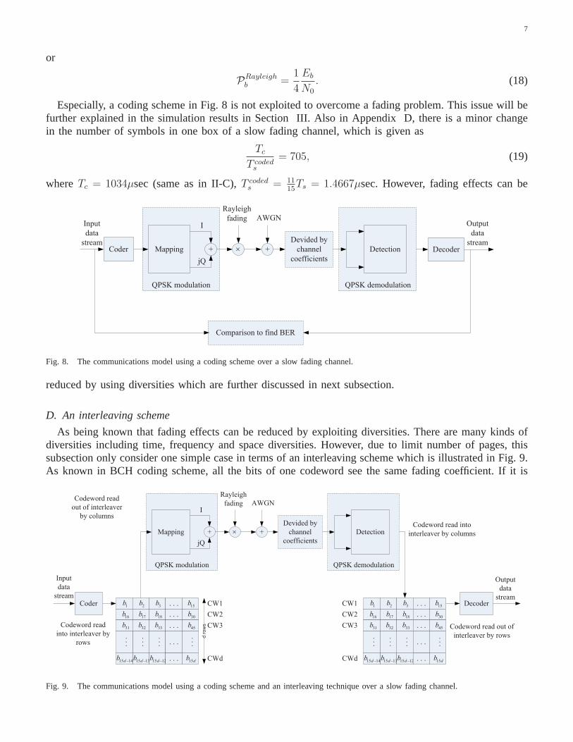
Especially, a coding scheme in Fig. 8 is not exploited to overcome a fading problem. This issue will befurther explained in the simulation results in Section III.Also in Appendix D, there is a minor changein the number of symbols in one box of a slow fading channel, which is given as
Tc
T codeds
= 705, (19)
whereTc = 1034µsec (same as in II-C),T codeds = 11
15Ts = 1.4667µsec. However, fading effects can be
QPSK demodulation
Mapping +
I
jQ
Input
data
stream+
AWGN
Detection
Output
data
stream
QPSK modulation
Comparison to find BER
Rayleigh
fading
Devided by
channel
coefficients
DecoderCoder
Fig. 8. The communications model using a coding scheme over a slow fading channel.
reduced by using diversities which are further discussed innext subsection.
D. An interleaving scheme
As being known that fading effects can be reduced by exploiting diversities. There are many kinds ofdiversities including time, frequency and space diversities. However, due to limit number of pages, thissubsection only consider one simple case in terms of an interleaving scheme which is illustrated in Fig. 9.As known in BCH coding scheme, all the bits of one codeword see the same fading coefficient. If it is
QPSK demodulation
Mapping +
I
jQ
Input
data
stream
+
AWGN
Detection
Output
data
stream
QPSK modulation
Rayleigh
fading
Devided by
channel
coefficients
DecoderCoder 1b 2b 3b
16b 17b 18b
31b 32b 33b
15 14db 15 13db 15 12db
. . .
. . .
. . .
15b
30b
45b
15db
. . .
. . .
. . .
. . .
. . .
. . .
d r
ow
s
CW1
CW2
CW3
CWd
Codeword read
into interleaver by
rows
Codeword read
out of interleaver
by columns
1b 2b 3b
16b 17b 18b
31b 32b 33b
15 14db 15 13db 15 12db
. . .
. . .
. . .
15b
30b
45b
15db
. . .
. . .
. . .
. . .
. . .
. . .
CW1
CW2
CW3
CWd
Codeword read into
interleaver by columns
Codeword read out of
interleaver by rows
Fig. 9. The communications model using a coding scheme and an interleaving technique over a slow fading channel.

8
affected by a specific deep fading box, all of them are corrupted. Because (15,11,1) BCH code can onlycorrect 1 error bit in each codeword. Furthermore, one fading box include 705 symbols. Hence if onespecific box is in deep fading, all symbols inside this duration are affected. So this code would add evenmore errors and the performance significantly degraded.
Motivated from this above feature, the smart scheme is proposed. It is good if different fading coefficientsare applied into different bits within a codeword. Hence, some of bits are affected by deep fading and theothers are still remained. As the results, error coding in terms of BCH coding can recover the receivedsignal. As seen in Fig. 9, each bit will be separated from the others in the same codeword byd− 1 bits.It is concluded that if this separation is larger than the channel coherence time, the fading affecting tocodewords is independent. It is handled by the following condition
d >Tc
T codedb
, (20)
whered is the deep of interleaving. So in a communications system, an interleaver is added before amodulator and a deinterleaver is added after a demodulator.
III. N UMERICAL RESULTS
0 1 2 3 4 5 6 7 810
−4
10−3
10−2
10−1
Eb/N
0, dB
Bit
Err
or R
ate
Bit error probability curve for QPSK
theory−QPSKsimulation−QPSK
Fig. 10. BER performance of a communications system using a QPSK modulation over an AWGN channel.
In this section, the simulation results are presented and further discussions are provided. Recall that thecommunications system uses QPSK modulation, and (15,11,1)BCH coding scheme. AWGN channel isfirst studied. Then Rayleigh fading channel is further examined due to the fact that the users are movingunder the condition of maximum moving speed,v = 81km/hour. The bit rate of communications systemis Rb = 1Mbps and the carrier frequency isfc = 5.4545GHz.
First of all, Fig. 10 illustrates the simulation results of the communications system over AWGN channel.It is clearly seen that the simulation and theoretical BERs arefitted.
Then, the coding scheme is added to communications system inorder to improve the performance interms of BER. In Fig. 11, BER of coding scheme is decreased significantly whenEb
N0
larger than7dB.For example, atEb
N0
= 8dB, BER for coding case is 10 times less than BER for without coding. However,at low Eb
N0
, coding does not work well. For instance, atEb
N0
= 0dB, BERs for coding and without codingcases are the same values.

9
0 1 2 3 4 5 6 7 8
10−6
10−4
10−2
100
Eb/N
0, dB
Bit
Err
or R
ate
Bit error probability curve for QPSK
theory−QPSKsimulation−QPSKtheory−QPSK−codingsimulation−QPSK−coding
Fig. 11. BER performance of a communications system using a QPSK modulation and a (15,11,1) BCH coding scheme over an AWGNchannel.
0 2 4 6 8 10 12 14 16 18 20
10−6
10−4
10−2
100
Eb/N
0, dB
Bit
Err
or R
ate
Bit error probability curve for QPSK
theory−QPSK−AWGNsimulation−QPSK−AWGNtheory−QPSK−fadingsimulation−QPSK−fading
Fig. 12. BER performance of a communications system using a QPSK modulation over a slow fading channel.
Now fading is considered. Fig. 12 shows the performance of communications system. It is easilyobserved that simulation BER is fitted with theoretical BER forthe case of fading channel. Also therelation between BER andEb
N0
(SNR) for the fading channel is a linear decrease while the relation forAWGN channel is an exponential decrease. It implies that although SNR is increased, BER performancefor fading channel is not much more improved. For example, even thoughEb
N0
= 20dB, BER of fadingchannel is still larger than10−3. So the need of technique to combat the fading effects is essential.
Let’s try to use coding scheme to overcome the fading effects. In Fig. 13, the results are not expected andsurprised. BER performance using coding is even dramatically degraded and higher than BER performancewithout using coding. It is due to the fact that when using coding, some boxes of fading channel aredeeply faded. Hence, all the whole codewords within these boxes get errors. Furthermore, BCH coding

10
0 2 4 6 8 10 12 14 16 18 20
10−6
10−4
10−2
100
Eb/N
0, dB
Bit
Err
or R
ate
Bit error probability curve for QPSK
simulation−QPSK−AWGNtheory−QPSK−AWGNtheory−QPSK−fadingsimulation−QPSK−fadingsimulation−QPSK−fading−coding
Fig. 13. BER performance of a communications system using a QPSK modulation and a (15,11,1) BCH coding scheme over a slow fadingchannel.
0 2 4 6 8 10 12 14 16 18 20
10−6
10−4
10−2
100
Eb/N
0, dB
Bit
Err
or R
ate
Bit error probability curve for QPSK
theory−QPSK−AWGNsimulation−QPSK−AWGNtheory−QPSK−fadingsimulation−QPSK−fadingsimulation−QPSK−fading−codingsimulation−QPSK−interleaver
Fig. 14. BER performance of a communications system using a QPSK modulation, a (15,11,1) BCH coding scheme and an interleavingtechnique over a slow fading channel.
can only correct one bit for each codeword and cannot recoverfor the case of burst errors above. As theresults, the errors are significantly increased in this case.
Motivated from finding solution for this above issue, an interleaving scheme which is one of the mostfamous diversity schemes is applied to a communications system. As seen in Fig. 14, an improvementis remarkably received. For example, atEb
N0
= 20dB, BER performance using an interleaver is 100 timesless than BER performance without using an interleaver. Alsoat this SNR, BER performance reach10−5
that is acceptable for a practical communications system.
11
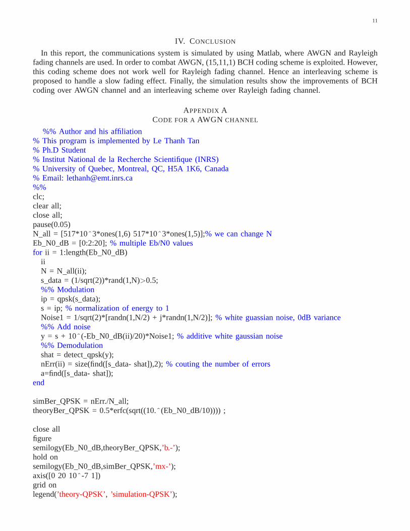
IV. CONCLUSION
In this report, the communications system is simulated by using Matlab, where AWGN and Rayleighfading channels are used. In order to combat AWGN, (15,11,1) BCHcoding scheme is exploited. However,this coding scheme does not work well for Rayleigh fading channel. Hence an interleaving scheme isproposed to handle a slow fading effect. Finally, the simulation results show the improvements of BCHcoding over AWGN channel and an interleaving scheme over Rayleigh fading channel.
APPENDIX ACODE FOR AAWGN CHANNEL
%% Author and his affiliation% This program is implemented by Le Thanh Tan% Ph.D Student% Institut National de la Recherche Scientifique (INRS)% University of Quebec, Montreal, QC, H5A 1K6, Canada% Email: [email protected]%%clc;clear all;close all;pause(0.05)N all = [517*10̂ 3*ones(1,6) 517*10̂3*ones(1,5)];% we can change NEb N0 dB = [0:2:20]; % multiple Eb/N0 valuesfor ii = 1:length(Eb N0 dB)
iiN = N all(ii);s data = (1/sqrt(2))*rand(1,N)>0.5;%% Modulationip = qpsk(s data);s = ip; % normalization of energy to 1Noise1 = 1/sqrt(2)*[randn(1,N/2) + j*randn(1,N/2)];% white guassian noise, 0dB variance%% Add noisey = s + 10̂ (-Eb N0 dB(ii)/20)*Noise1;% additive white gaussian noise%% Demodulationshat = detectqpsk(y);nErr(ii) = size(find([s data- shat]),2);% couting the number of errorsa=find([s data- shat]);
end
simBer QPSK = nErr./Nall;theoryBer QPSK = 0.5*erfc(sqrt((10.ˆ (Eb N0 dB/10)))) ;
close allfiguresemilogy(EbN0 dB,theoryBerQPSK,’b.-’ );hold onsemilogy(EbN0 dB,simBer QPSK,’mx-’ );axis([0 20 10̂ -7 1])grid onlegend(’theory-QPSK’, ’simulation-QPSK’);

12
xlabel(’Es/No, dB’)ylabel(’Bit Error Rate’)title(’Bit error probability curve for QPSK’)save Quesadata simBerQPSK theoryBerQPSK Eb N0 dB% save Quesadata1 simBerQPSK theoryBerQPSK Eb N0 dB
where ’qpsk.m’ is%% Author and his affiliation
% This program is implemented by Le Thanh Tan% Ph.D Student% Institut National de la Recherche Scientifique (INRS)% University of Quebec, Montreal, QC, H5A 1K6, Canada% Email: [email protected]%%function d = qpsk(b)% ˆ% —% 10 x — x 00 (odd bit, even bit)% —% ——-+——-> real part (I channel)% —% 11 x — x 01% —%% Input:% b = bits{0, 1} to be mapped into QPSK symbols%% Output:% d = complex-valued QPSK symbolsfor i =1:length(b)/2
if b(2*i-1)==1d(i) =1 ;
elsed(i) = -1;endif b(2*i)==1
d(i)=d(i)+j;elsed(i)=d(i)-j;end
end
and ’detectqpsk.m’ is%% Author and his affiliation% This program is implemented by Le Thanh Tan% Ph.D Student% Institut National de la Recherche Scientifique (INRS)% University of Quebec, Montreal, QC, H5A 1K6, Canada% Email: [email protected]%%

13
function bhat = detect(r)
% Assumed mapping:%% 10 x — x 00% —% ——-+——-% —% 11 x — x 01%% Input:% r = sequence of complex-valued QPSK symbols%% Output:% bhat = bits{0,1} corresponding to the QPSK symbolsL = length(r);bhat =[];for i=1:L
if real(r(i))>=0if imag(r(i))>=0
bhat = [bhat,[1,1]];elsebhat = [bhat,[1,0]];end
elseif imag(r(i))>=0
bhat = [bhat,[0,1]];elsebhat = [bhat,[0,0]];end
endend
APPENDIX BCODE FOR AAWGN CHANNEL AND A BCH CODING
%% Author and his affiliation% This program is implemented by Le Thanh Tan% Ph.D Student% Institut National de la Recherche Scientifique (INRS)% University of Quebec, Montreal, QC, H5A 1K6, Canada% Email: [email protected]%%clc;clear all;close all;pause(0.05)N all = [517*10̂ 3*ones(1,6) 517*10̂3*ones(1,5)];% we can change NEb N0 dB = [0:2:20]; % multiple Eb/N0 values%% Prepare for coder and decoder
k=11;

14
n=15;g1=[1 0 0 1 1];G=Gformulation(k,g1);g=[1 0 0 1 1 0 0 0 0 0 0 0 0 0 0];r=n-k;H=Hformulation(k,G,r);HT=H.’;for ii = 1:length(Eb N0 dB)
iiN = N all(ii);s data = (1/sqrt(2))*rand(1,N)>0.5;% normalization of energy to 1s data1 = reshape(sdata,11,floor(N/11))’;for i=1:size(s data1,1),
tan temp = s data1(i,:)*G;tan temp = mod(tantemp,2);bch1(i,:) = tantemp;
ends data2 = reshape(bch1’,1,size(bch1,1)*size(bch1,2));%% QPSK modulationip = qpsk(s data2);s = ip;N1 = length(s);Noise1 = 1/sqrt(2)*[randn(1,N1) + j*randn(1,N1)];% white guassian noise, 0dB variance
y = s + sqrt(n/k)*10̂ (-Eb N0 dB(ii)/20)*Noise1;% additive white gaussian noise%% QPSK demodulationshat = detectqpsk(y);%% decodershat1 = reshape(shat,15,floor(length(shat)/15))’;for i=1:size(shat1,1),
bch2(i,:)=syndtan(shat1(i,:),g,HT);bch3(i,1:11)=bch2(i,1:11);
endshat2 = reshape(bch3’,1,size(bch3,1)*size(bch3,2));%% Error number calculationnErr(ii) = size(find([s data- shat2]),2);% couting the number of errorsa=find([s data- shat2]);
endsimBer QPSK = nErr./Nall;P nocode = 0.5*erfc(sqrt((k/n*10.ˆ (Eb N0 dB/10))));for i =2:n,
Ptem(i,:)=i*nchoosek(n,i)*(Pnocode.̂ i).*((1-P nocode).̂ (n-i));endtheoryBer QPSK = 1/n* sum(Ptem);figuresemilogy(EbN0 dB,theoryBerQPSK,’b.-’ );hold onsemilogy(EbN0 dB,simBer QPSK,’mx-’ );axis([0 20 10̂ -7 1])

15
grid onlegend(’theory-QPSK-coding’, ’simulation-QPSK-coding’);xlabel(’Es/No, dB’)ylabel(’Bit Error Rate’)title(’Bit error probability curve for QPSK’)save Quesbdata simBerQPSK theoryBerQPSK Eb N0 dB
where ’Gformulation.m’ is%% Author and his affiliation
% This program is implemented by Le Thanh Tan% Ph.D Student% Institut National de la Recherche Scientifique (INRS)% University of Quebec, Montreal, QC, H5A 1K6, Canada% Email: [email protected] G=Gformulation(k,g)row=k;n=length(g);col=row-1+n;A=zeros(row,col);A(end,row:end)=g;
for i=1:row-1A(end-i,row-i:end-i)=A(end,row:end);
endfor j=row:-1:2
for i=j-1:-1:1if(A(i,j) >0)C1=A(i,:);C2=A(j,:);C=C1+C2;B=mod(C,2);A(i,:)=B;
endclear C1 C2 C B
endendG=A;
’Hformulation.m’ is%% Author and his affiliation
% This program is implemented by Le Thanh Tan% Ph.D Student% Institut National de la Recherche Scientifique (INRS)% University of Quebec, Montreal, QC, H5A 1K6, Canada% Email: [email protected] H=Hformulation(k,G,r)G1=G(:,end-r+1:end);G1=G1’;

16
Ir=eye(r);H=[G1,Ir];
’synd tan.m’ is%% Author and his affiliation
% This program is implemented by Le Thanh Tan% Ph.D Student% Institut National de la Recherche Scientifique (INRS)% University of Quebec, Montreal, QC, H5A 1K6, Canada% Email: [email protected][bch]=syndtan(data,G,HT)k=0;for i=1:15
if data(i)==1k=i;break
endendg=circshift(G,[0 k-1]);g1=g;c=data;for n=1:15
c=xor(c,g1);h=0;for i=1:15
if c(i)==0h=h+1;
endendif h==15
breakendg1=G;for i=1:15
if c(i)==1kk=i;break
endendif kk>11
breakendg1=circshift(g1,[0 kk-1]);
endk1=0;for i=1:15
if c(i)==1k1=k1+1;
end

17
endif k1==0
bch=data;else
for i=1:4s(i)=c(11+i);
endfor j=1:15
ht(j,:)=xor(s,HT(j,:));k2=0;for i=1:4;
if ht(j,i)==0k2=k2+1;
endif k2==4
k3=j;break
endend
endfor i=1:15
e(i)=0;ende(k3)=1;bch=xor(data,e);
end
APPENDIX CCODE FOR ARAYLEIGH CHANNEL
%% Author and his affiliation% This program is implemented by Le Thanh Tan% Ph.D Student% Institut National de la Recherche Scientifique (INRS)% University of Quebec, Montreal, QC, H5A 1K6, Canada% Email: [email protected]%%clc;clear all;close all;pause(0.05)N all = [517*10̂ 3*ones(1,6) 517*10̂3*ones(1,5)];% we can change NEb N0 dB = [0:2:20]; % multiple Eb/N0 valuesfor ii = 1:length(Eb N0 dB)
iiN = N all(ii);s data = (1/sqrt(2))*rand(1,N)>0.5;%% Modulationip = qpsk(s data);

18
s = ip; % normalization of energy to 1Noise1 = 1/sqrt(2)*[randn(1,N/2) + j*randn(1,N/2)];% white guassian noise, 0dB varianceh = 1/sqrt(2)*[randn(1,N/2/517) + j*randn(1,N/2/517)];% Rayleigh channelh = h’*ones(1,517);h = reshape(h’,1,size(h,1)*size(h,2));%% Add noisey = h.*s + 10̂ (-Eb N0 dB(ii)/20)*Noise1;% additive white gaussian noise%% Equalizationyeq = y./h;%% Demodulationshat = detectqpsk(yeq);nErr(ii) = size(find([s data- shat]),2);% couting the number of errorsa=find([s data- shat]);
endsimBer QPSK = nErr./Nall;EbN0Lin = 10.̂ (Eb N0 dB/10);theoryBer QPSK = 0.5.*(1-sqrt(EbN0Lin./(EbN0Lin+1)));theoryBerAWGN = 0.5*erfc(sqrt(10.ˆ (Eb N0 dB/10)));close allfiguresemilogy(EbN0 dB,theoryBerQPSK,’b.-’ );hold onsemilogy(EbN0 dB,simBer QPSK,’mx-’ );hold onsemilogy(EbN0 dB,theoryBerAWGN,’r*-’ );axis([0 20 10̂ -7 1])grid onlegend(’theory-QPSK-fading’, ’simulation-QPSK-fading’,’theory-QPSK-AWGN’);xlabel(’Es/No, dB’)ylabel(’Bit Error Rate’)title(’Bit error probability curve for QPSK’)save Quescdata simBerQPSK theoryBerQPSK theoryBerAWGN EbN0 dB
APPENDIX DCODE FOR ARAYLEIGH CHANNEL AND A BCH CODING
%% Author and his affiliation% This program is implemented by Le Thanh Tan% Ph.D Student% Institut National de la Recherche Scientifique (INRS)% University of Quebec, Montreal, QC, H5A 1K6, Canada% Email: [email protected]%%clc;clear all;close all;pause(0.05)N all = [517*10̂ 3*ones(1,6) 517*10̂3*ones(1,5)];% we can change NEb N0 dB = [0:2:20]; % multiple Eb/N0 values

19
%% Prepare for coder and decoderk=11;n=15;g1=[1 0 0 1 1];G=Gformulation(k,g1);g=[1 0 0 1 1 0 0 0 0 0 0 0 0 0 0];r=n-k;H=Hformulation(k,G,r);HT=H.’;for ii = 1:length(Eb N0 dB)
iiN = N all(ii);s data = (1/sqrt(2))*rand(1,N)>0.5;% normalization of energy to 1s data1 = reshape(sdata,11,floor(N/11))’;for i=1:size(s data1,1),
tan temp = s data1(i,:)*G;tan temp = mod(tantemp,2);bch1(i,:) = tantemp;
ends data2 = reshape(bch1’,1,size(bch1,1)*size(bch1,2));%% QPSK Modulationip = qpsk(s data2);s = ip; % normalization of energy to 1N1 = length(s);Noise1 = 1/sqrt(2)*[randn(1,N1) + j*randn(1,N1)];% white guassian noise, 0dB varianceh = 1/sqrt(2)*[randn(1,floor(N1/705)) + j*randn(1,floor(N1/705))]; % Rayleigh channelta temp = h(end);h = h’*ones(1,705);h = reshape(h’,1,size(h,1)*size(h,2));h = [h ta temp*ones(1,N1-length(h))];% use when the lengths of h and data are not equal%% Add noisey = h.*s + sqrt(n/k)*10̂ (-Eb N0 dB(ii)/20)*Noise1;% additive white gaussian noise%% Equalizationyeq = y./h;%% QPSK Demodulationshat = detectqpsk(yeq);%% decodershat1 = reshape(shat,15,floor(length(shat)/15))’;for i=1:size(shat1,1),
bch2(i,:)=syndtan(shat1(i,:),g,HT);bch3(i,1:11)=bch2(i,1:11);
endshat2 = reshape(bch3’,1,size(bch3,1)*size(bch3,2));%% Error number calculationnErr(ii) = size(find([s data- shat2]),2);% couting the number of errorsa=find([s data- shat2]);
endsimBer QPSK = nErr./Nall;EbN0Lin = 10.̂ (Eb N0 dB/10);

20
theoryBer QPSK = 0.5.*(1-sqrt(EbN0Lin./(EbN0Lin+1)));theoryBerAWGN = 0.5*erfc(sqrt(10.ˆ (Eb N0 dB/10)));close allfiguresemilogy(EbN0 dB,theoryBerQPSK,’b.-’ );hold onsemilogy(EbN0 dB,simBer QPSK,’mx-’ );hold onsemilogy(EbN0 dB,theoryBerAWGN,’r*-’ );axis([0 20 10̂ -7 1])grid onlegend(’theory-QPSK-fading’, ’simulation-QPSK-fading-coding’,’theory-QPSK-AWGN’);xlabel(’Es/No, dB’)ylabel(’Bit Error Rate’)title(’Bit error probability curve for QPSK’)save Quesddata simBerQPSK theoryBerQPSK theoryBerAWGN EbN0 dB
APPENDIX ECODE FOR ARAYLEIGH CHANNEL , A BCH CODING AND AN INTERLEAVING SCHEME
%% Author and his affiliation% This program is implemented by Le Thanh Tan% Ph.D Student% Institut National de la Recherche Scientifique (INRS)% University of Quebec, Montreal, QC, H5A 1K6, Canada% Email: [email protected]%%clc;clear all;close all;pause(0.05)N all = [517*10̂ 3*ones(1,6) 517*10̂3*ones(1,5)];% we can change NEb N0 dB = [0:2:20]; % multiple Eb/N0 values%% Prepare for coder and decoder
k=11;n=15;g1=[1 0 0 1 1];G=Gformulation(k,g1);g=[1 0 0 1 1 0 0 0 0 0 0 0 0 0 0];r=n-k;H=Hformulation(k,G,r);HT=H.’;for ii = 1:length(Eb N0 dB)
iiN = N all(ii);s data = (1/sqrt(2))*rand(1,N)>0.5;% normalization of energy to 1s data1 = reshape(sdata,11,floor(N/11))’;for i=1:size(s data1,1),
tan temp = s data1(i,:)*G;

21
tan temp = mod(tantemp,2);bch1(i,:) = tantemp;
end%% Interleavers data2 = reshape(bch1,1,size(bch1,1)*size(bch1,2));%read out by column%% QPSK Modulationip = qpsk(s data2);s = ip; % normalization of energy to 1N1 = length(s);Noise1 = 1/sqrt(2)*[randn(1,N1) + j*randn(1,N1)];% white guassian noise, 0dB varianceh = 1/sqrt(2)*[randn(1,floor(N1/705)) + j*randn(1,floor(N1/705))]; % Rayleigh channelh = h’*ones(1,705);ta temp = h(end);h = reshape(h’,1,size(h,1)*size(h,2));h = [h ta temp*ones(1,N1-length(h))];% use when the lengths of h and data are not equal%% Add noisey = h.*s + 10̂ (-Eb N0 dB(ii)/20)*Noise1;% additive white gaussian noise%% Equalizationyeq = y./h;%% QPSK Demodulationshat = detectqpsk(yeq);%% decodershat1 = reshape(shat,floor(length(shat)/15),15);for i=1:size(shat1,1),
bch2(i,:)=syndtan(shat1(i,:),g,HT);bch3(i,1:11)=bch2(i,1:11);
endshat2 = reshape(bch3’,1,size(bch3,1)*size(bch3,2));%% Error number calculationnErr(ii) = size(find([s data- shat2]),2);% couting the number of errorsa=find([s data- shat2]);
endsimBer QPSK = nErr./Nall;EbN0Lin = 10.̂ (Eb N0 dB/10);theoryBer QPSK = 0.5.*(1-sqrt(EbN0Lin./(EbN0Lin+1)));theoryBerAWGN = 0.5*erfc(sqrt(10.ˆ (Eb N0 dB/10)));close allfiguresemilogy(EbN0 dB,theoryBerQPSK,’b.-’ );hold onsemilogy(EbN0 dB,simBer QPSK,’mx-’ );hold onsemilogy(EbN0 dB,theoryBerAWGN,’r*-’ );axis([0 20 10̂ -7 1])grid onlegend(’theory-QPSK-fading’, ’simulation-QPSK-interleaver’,’theory-QPSK-AWGN’);xlabel(’Es/No, dB’)ylabel(’Bit Error Rate’)title(’Bit error probability curve for QPSK’)

22
save Quesedata simBerQPSK theoryBerQPSK theoryBerAWGN EbN0 dB
REFERENCES
[1] John G. Proakis, Digital Communications, 4th Edition, McGrawHill, 2000.[2] B. Sklar, Digital communications : fundamentals and applications, 2nded., Upper Saddle River, N.J.: Prentice-Hall PTR, 2001.[3] T. S. Rappaport, Wireless communications : principles and practice,2nd ed., Upper Saddle River, N.J.: Prentice Hall PTR, 2002.
Recommended


