IntroductionIntroduction
Minimizing energy consumption is crucial for computing Minimizing energy consumption is crucial for computing
systemssystems Battery operated systemsBattery operated systems
Data centersData centers
Wide variety of techniques have been proposedWide variety of techniques have been proposed Static (Offline) optimizationsStatic (Offline) optimizations
• Compiler optimizationsCompiler optimizations• AcceleratorsAccelerators
Dynamic (Online) optimizationsDynamic (Online) optimizations• OS schedulingOS scheduling• C-state management in Intel processorsC-state management in Intel processors 1
IntroductionIntroduction
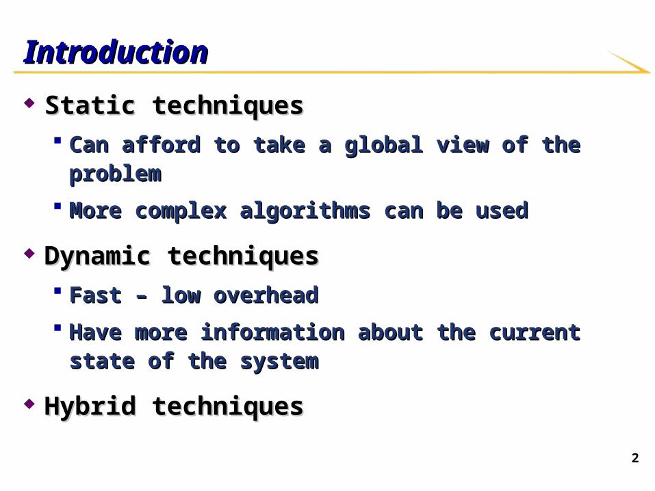
Static techniquesStatic techniques Can afford to take a global view of the problemCan afford to take a global view of the problem
More complex algorithms can be usedMore complex algorithms can be used
Dynamic techniquesDynamic techniques Fast – low overheadFast – low overhead
Have more information about the current state of the systemHave more information about the current state of the system
Hybrid techniquesHybrid techniques
2
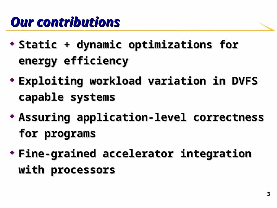
Our contributionsOur contributions
Static + dynamic optimizations for energy efficiency Static + dynamic optimizations for energy efficiency
Exploiting workload variation in DVFS capable systems Exploiting workload variation in DVFS capable systems
Assuring application-level correctness for programsAssuring application-level correctness for programs
Fine-grained accelerator integration with processorsFine-grained accelerator integration with processors
3
Energy efficient multiprocessor task scheduling under Energy efficient multiprocessor task scheduling under input-dependent variationinput-dependent variation
5
OutlineOutline
Introduction and motivationIntroduction and motivation
Related workRelated work
Problem formulationProblem formulation
Proposed algorithmProposed algorithm
Experimental resultsExperimental results

6
Introduction and MotivationIntroduction and Motivation Embedded systems are typically required to meet a fixed Embedded systems are typically required to meet a fixed
performance targetperformance target Example – frame rate for decoding of streaming videoExample – frame rate for decoding of streaming video
A system that has better performance provides no significant benefit A system that has better performance provides no significant benefit
Dynamic Voltage + Frequency Scaling (DVFS) is an effective Dynamic Voltage + Frequency Scaling (DVFS) is an effective
technique for reducing dynamic energy consumption of processorstechnique for reducing dynamic energy consumption of processors Quadratic dependence of energy on voltage (almost)Quadratic dependence of energy on voltage (almost)
Linear dependence of performance (frequency) on voltage (almost)Linear dependence of performance (frequency) on voltage (almost)
7
IntroductionIntroduction DVFS problem: Given a task graph DVFS problem: Given a task graph G:G:
Edges - precedence constraints, Edges - precedence constraints, Latency constraint Latency constraint LL Determine the Determine the scheduleschedule and and voltage assignmentvoltage assignment for each task to for each task to
minimize energy consumptionminimize energy consumption
Traditional techniques consider worst-case computation Traditional techniques consider worst-case computation time of every tasktime of every task Ensures that the latency constraint is satisfied.Ensures that the latency constraint is satisfied.
Real-world applications exhibit significant variation in Real-world applications exhibit significant variation in execution times.execution times.
8
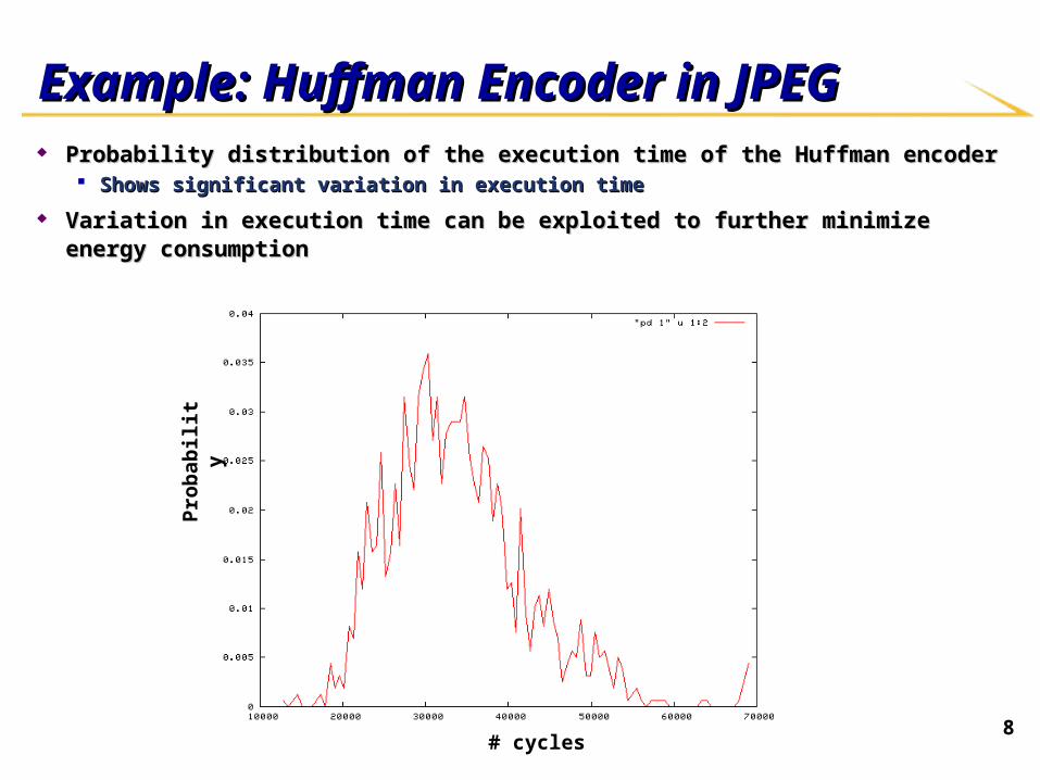
Example: Huffman Encoder in JPEGExample: Huffman Encoder in JPEG Probability distribution of the execution time of the Huffman encoderProbability distribution of the execution time of the Huffman encoder
Shows significant variation in execution timeShows significant variation in execution time
Variation in execution time can be exploited to further minimize energy consumptionVariation in execution time can be exploited to further minimize energy consumption
# cycles
Pro
bab
ilit
y

9
Example – Energy Consumption in Worst-case and Example – Energy Consumption in Worst-case and Typical CaseTypical CaseUsing equations based on CMOS for modeling relation Using equations based on CMOS for modeling relation
between energy, frequency and voltagebetween energy, frequency and voltage
WorkloadWorkload - # cycles that a task takes to complete - # cycles that a task takes to complete
Input dependentInput dependent
4 processor system - Latency constraint of 300 time units4 processor system - Latency constraint of 300 time units
Worst-case scheduling – 1 time unit for clock period of Worst-case scheduling – 1 time unit for clock period of
each taskeach task
Energy consumption 400*CEnergy consumption 400*C
Typical case – 75 cycles per taskTypical case – 75 cycles per task
Energy consumption 168.75*CEnergy consumption 168.75*C
Potentially 58% reduction in energy!Potentially 58% reduction in energy!
WorkLoad(v) (cycles)
Probability
75 0.70 100 0.30
v4
v2 v3
v1
22
C*WE C*W * f
( cp )

10
OutlineOutline
Introduction and motivationIntroduction and motivation
Related workRelated work
Problem formulationProblem formulation
Proposed algorithmProposed algorithm
Experimental resultsExperimental results
11
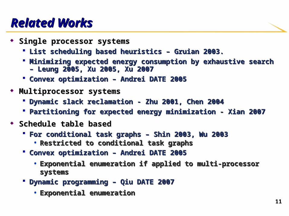
Related WorksRelated Works Single processor systemsSingle processor systems
List scheduling based heuristics – Gruian 2003.List scheduling based heuristics – Gruian 2003. Minimizing expected energy consumption by exhaustive search – Leung 2005, Xu 2005, Minimizing expected energy consumption by exhaustive search – Leung 2005, Xu 2005,
Xu 2007Xu 2007 Convex optimization – Andrei DATE 2005Convex optimization – Andrei DATE 2005
Multiprocessor systemsMultiprocessor systems Dynamic slack reclamation - Zhu 2001, Chen 2004Dynamic slack reclamation - Zhu 2001, Chen 2004 Partitioning for expected energy minimization - Xian 2007Partitioning for expected energy minimization - Xian 2007
Schedule table basedSchedule table based For conditional task graphs – Shin 2003, Wu 2003For conditional task graphs – Shin 2003, Wu 2003
• Restricted to conditional task graphsRestricted to conditional task graphs Convex optimization – Andrei DATE 2005Convex optimization – Andrei DATE 2005
• Exponential enumeration if applied to multi-processor systemsExponential enumeration if applied to multi-processor systems Dynamic programming – Qiu DATE 2007Dynamic programming – Qiu DATE 2007
• Exponential enumerationExponential enumeration
12
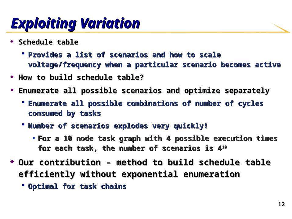
Exploiting VariationExploiting Variation Schedule tableSchedule table
Provides a list of scenarios and how to scale voltage/frequency when a Provides a list of scenarios and how to scale voltage/frequency when a
particular scenario becomes activeparticular scenario becomes active
How to build schedule table?How to build schedule table?
Enumerate all possible scenarios and optimize separatelyEnumerate all possible scenarios and optimize separately
Enumerate all possible combinations of number of cycles consumed by tasksEnumerate all possible combinations of number of cycles consumed by tasks
Number of scenarios explodes very quickly!Number of scenarios explodes very quickly!
• For a 10 node task graph with 4 possible execution times for each task, the For a 10 node task graph with 4 possible execution times for each task, the
number of scenarios is 4number of scenarios is 41010
Our contribution – method to build schedule table efficiently without Our contribution – method to build schedule table efficiently without
exponential enumerationexponential enumeration Optimal for task chainsOptimal for task chains

13
Processor and Application ModelProcessor and Application Model Processor modelProcessor model
Homogeneous multiprocessor systemHomogeneous multiprocessor system
Voltage of each processor can be tuned independently in the range [Voltage of each processor can be tuned independently in the range [VVlowerlower, V, Vupperupper]]
Use quadratic approximation to model relation between energy and frequency Use quadratic approximation to model relation between energy and frequency
Application modelApplication model Task graph Task graph GG with nodes representing tasks with nodes representing tasks
Edges represent precedence constraintsEdges represent precedence constraints
Mapping of tasks to processors assumed to be givenMapping of tasks to processors assumed to be given• If not, use a priority based mapping heuristicIf not, use a priority based mapping heuristic
1th(V V )
f CV
22E C WV 2 3
3 2
C WE C Wf
( cp )
14
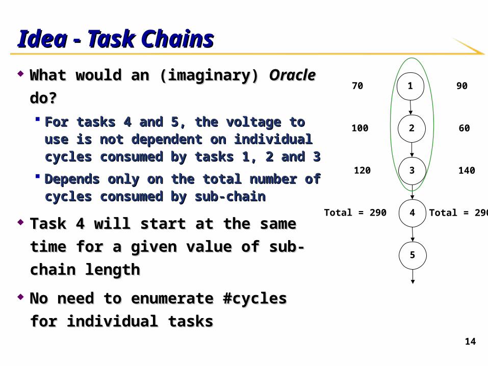
Idea - Task ChainsIdea - Task Chains
What would an (imaginary) What would an (imaginary) OracleOracle do? do? For tasks 4 and 5, the voltage to use is not For tasks 4 and 5, the voltage to use is not
dependent on individual cycles consumed dependent on individual cycles consumed by tasks 1, 2 and 3by tasks 1, 2 and 3
Depends only on the total number of Depends only on the total number of cycles consumed by sub-chaincycles consumed by sub-chain
Task 4 will start at the same time for a Task 4 will start at the same time for a
given value of sub-chain lengthgiven value of sub-chain length
No need to enumerate #cycles for No need to enumerate #cycles for
individual tasksindividual tasks
1
2
3
4
5
70
100
120
90
60
140
Total = 290 Total = 290
15
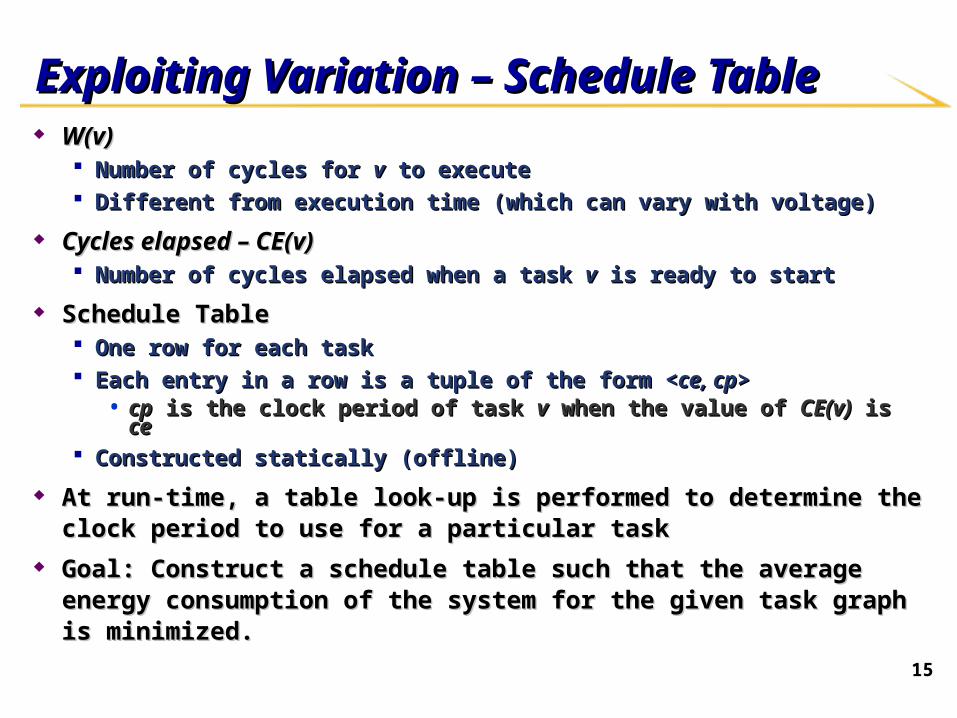
Exploiting Variation – Schedule TableExploiting Variation – Schedule Table W(v)W(v)
Number of cycles for Number of cycles for vv to execute to execute Different from execution time (which can vary with voltage)Different from execution time (which can vary with voltage)
Cycles elapsed – CE(v)Cycles elapsed – CE(v) Number of cycles elapsed when a task Number of cycles elapsed when a task vv is ready to start is ready to start
Schedule TableSchedule Table One row for each taskOne row for each task Each entry in a row is a tuple of the form <Each entry in a row is a tuple of the form <ce, cpce, cp>>
• cpcp is the clock period of task is the clock period of task vv when the value of when the value of CE(v)CE(v) is is cece Constructed statically (offline)Constructed statically (offline)
At run-time, a table look-up is performed to determine the clock period to use for a At run-time, a table look-up is performed to determine the clock period to use for a particular taskparticular task
Goal: Construct a schedule table such that the average energy consumption of the Goal: Construct a schedule table such that the average energy consumption of the system for the given task graph is minimized.system for the given task graph is minimized.
16
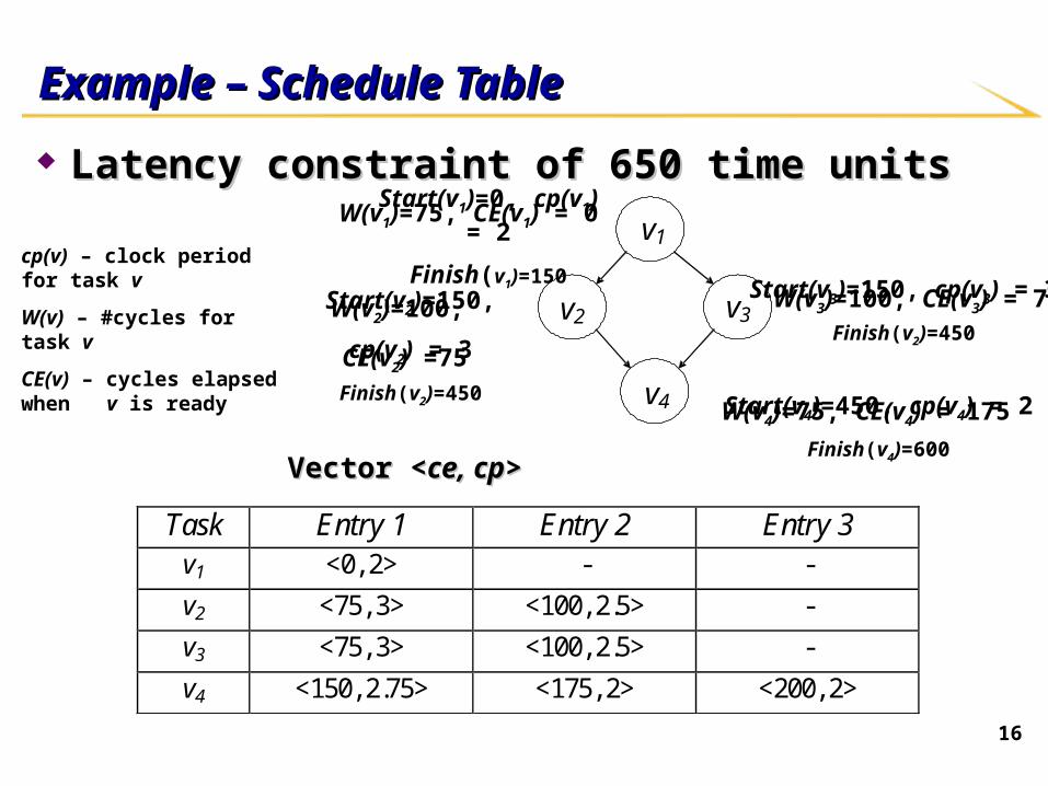
Example – Schedule TableExample – Schedule Table
Latency constraint of 650 time unitsLatency constraint of 650 time units
Task Entry 1 Entry 2 Entry 3 v1 <0, 2> - -
v2 <75, 3> <100, 2.5> -
v3 <75, 3> <100, 2.5> -
v4 <150, 2.75> <175, 2> <200, 2>
cp(v) – clock period for task v
W(v) – #cycles for task v
CE(v) – cycles elapsed when v is ready
v4
v2 v3
v1 W(v1)=75, CE(v1) = 0
Start(v1)=0, cp(v1) = 2
Finish(v1)=150
W(v2)=100,
CE(v2) =75
Start(v3)=150, cp(v3) = 3
Finish(v2)=450
W(v3)=100, CE(v3) = 75Start(v2)=150,
cp(v2) = 3
Finish(v2)=450W(v4)=75, CE(v4) = 175Start(v4)=450, cp(v4) = 2
Finish(v4)=600Vector <Vector <ce, cpce, cp>>
17
Constructing the Schedule TableConstructing the Schedule Table Based on J. Cong, W. Jiang and Z. Zhang ASP-DAC’07 formulationBased on J. Cong, W. Jiang and Z. Zhang ASP-DAC’07 formulation
Time budgeting for operations to minimize energy consumption in high level Time budgeting for operations to minimize energy consumption in high level synthesissynthesis
Latency constraintLatency constraint
Variable definitionsVariable definitions bbii is the latency of task is the latency of task ii ssi i is the start time of task is the start time of task ii cp(i)cp(i) is the clock period to use while running task is the clock period to use while running task II
Convex optimization with linear constraintsConvex optimization with linear constraints Does not consider variation in latency of individual operationsDoes not consider variation in latency of individual operations
18
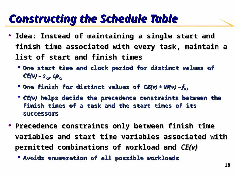
Constructing the Schedule TableConstructing the Schedule Table Idea: Instead of maintaining a single start and finish time associated Idea: Instead of maintaining a single start and finish time associated
with every task, maintain a list of start and finish timeswith every task, maintain a list of start and finish times One start time and clock period for distinct values of One start time and clock period for distinct values of CE(v) – sCE(v) – sv,jv,j, cp, cpv,jv,j
One finish for distinct values of One finish for distinct values of CE(v) + W(v) – fCE(v) + W(v) – fv,jv,j
CE(v)CE(v) helps decide the precedence constraints between the finish times of a helps decide the precedence constraints between the finish times of a task and the start times of its successorstask and the start times of its successors
Precedence constraints only between finish time variables and start Precedence constraints only between finish time variables and start
time variables associated with permitted combinations of workload time variables associated with permitted combinations of workload
and and CE(v)CE(v) Avoids enumeration of all possible workloadsAvoids enumeration of all possible workloads

19
Constructing the Schedule TableConstructing the Schedule Table
v1v1
v2v2
v4v4
v3v3
f1 = Finish time ofv1 when v1 takes 75 cycles
f1 = Finish time ofv1 when v1 takes 75 cycles
s1 = Start time of v2 when v1 takes 75 cycles
s1 = Start time of v2 when v1 takes 75 cycles
Precedence constraints1 ≥ f1
Precedence constraints1 ≥ f1
s2 = Start time of v2 when v1 takes 100 cycles
s2 = Start time of v2 when v1 takes 100 cycles
f2 = Finish time ofv1 when v1 takes 100 cycles
f2 = Finish time ofv1 when v1 takes 100 cycles
s2 ≥ f2s2 ≥ f2
No constraint needed between f2 and s1 !No constraint needed between f2 and s1 !
Each task maintains a list Each task maintains a list
of start and finish timesof start and finish times
Each start time (and Each start time (and
finish time) is associated finish time) is associated
with the number of with the number of
cycles elapsed.cycles elapsed.
Constraints imposed Constraints imposed
only on valid only on valid
combinations of start combinations of start
and finish times.and finish times.
v2 can start earlier if v1 takes 75 cycles!
v2 can start earlier if v1 takes 75 cycles!
20
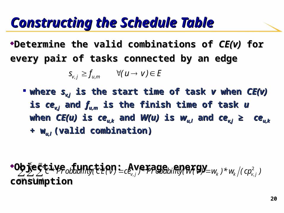
Constructing the Schedule TableConstructing the Schedule TableDetermine the valid combinations of Determine the valid combinations of CE(v)CE(v) for every pair of tasks for every pair of tasks
connected by an edgeconnected by an edge
where where ssv,jv,j is the start time of task is the start time of task vv when when CE(v)CE(v) is is cecev,jv,j and and ffu,mu,m is the is the
finish time of task finish time of task uu when when CE(u)CE(u) is is ceceu,ku,k and and W(u)W(u) is is wwu,lu,l and and cecev,jv,j ≥ ≥ ceceu,ku,k
+ w+ wu,lu,l (valid combination)(valid combination)
Objective function: Average energy consumptionObjective function: Average energy consumption
v , j u ,ms f ( u v ) E
2
1 1
K m
v, j k k v , jv V j k
C* Pr obability( CE( v ) ce )* Pr obability(W( v ) w )* w ( cp )

21
Determining the Values of CE(v)Determining the Values of CE(v)To keep the problem size from To keep the problem size from exploding, we keep a constant number exploding, we keep a constant number of values (of values (KK) of ) of CE(v)CE(v) at each task at each task
Profiling to determine the probability Profiling to determine the probability distribution of workload of a task distribution of workload of a task vv and and CE(v)CE(v)
Heuristics to determine values of Heuristics to determine values of CE(v)CE(v) to use at each nodeto use at each node
Divide the range of Divide the range of CE(v)CE(v) into into KK equal partsequal parts
Divide the area under the Divide the area under the probability v/s probability v/s CE(v)CE(v) graph into graph into KK equal regions equal regions
# cycles
Pro
bab
ilit
y
K=5
2
1 1
K m
v, j k k v , jv V j k
C* Pr obability( CE( v ) ce )* Pr obability(W( v ) w )* w ( cp )
22
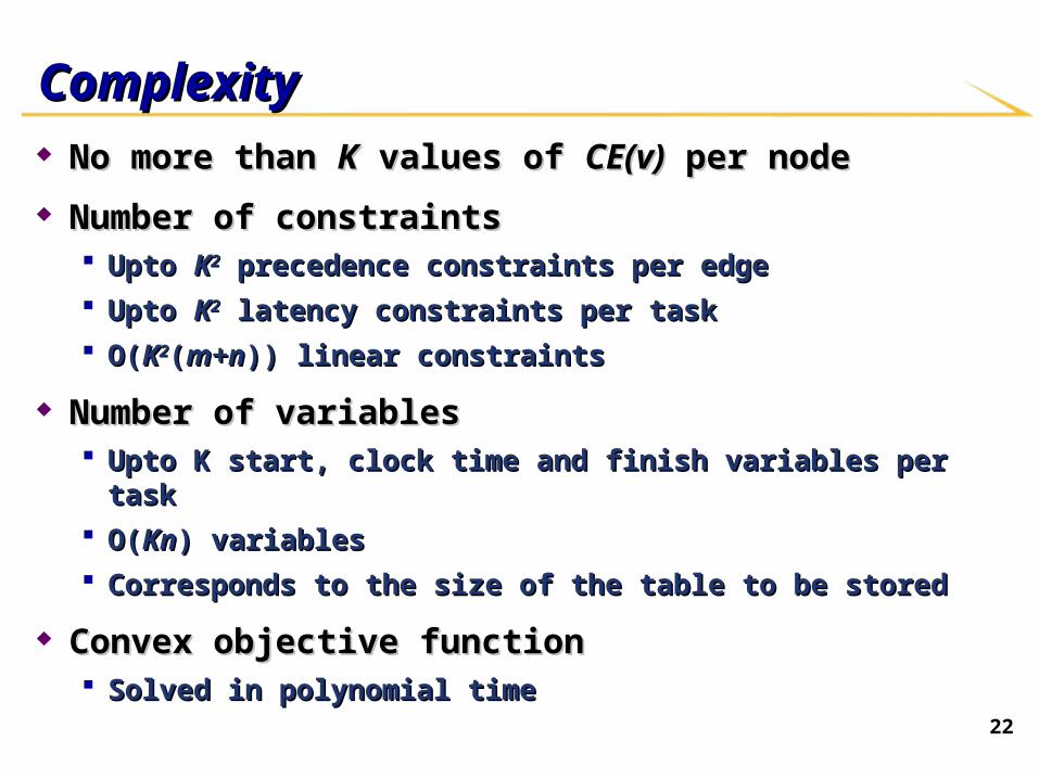
ComplexityComplexity No more than No more than KK values of values of CE(v)CE(v) per node per node
Number of constraintsNumber of constraints Upto Upto KK22 precedence constraints per edge precedence constraints per edge
Upto Upto KK22 latency constraints per task latency constraints per task
O(O(KK22((m+nm+n)) linear constraints)) linear constraints
Number of variablesNumber of variables Upto K start, clock time and finish variables per taskUpto K start, clock time and finish variables per task
O(O(KnKn) variables) variables
Corresponds to the size of the table to be storedCorresponds to the size of the table to be stored
Convex objective functionConvex objective function Solved in polynomial timeSolved in polynomial time
23
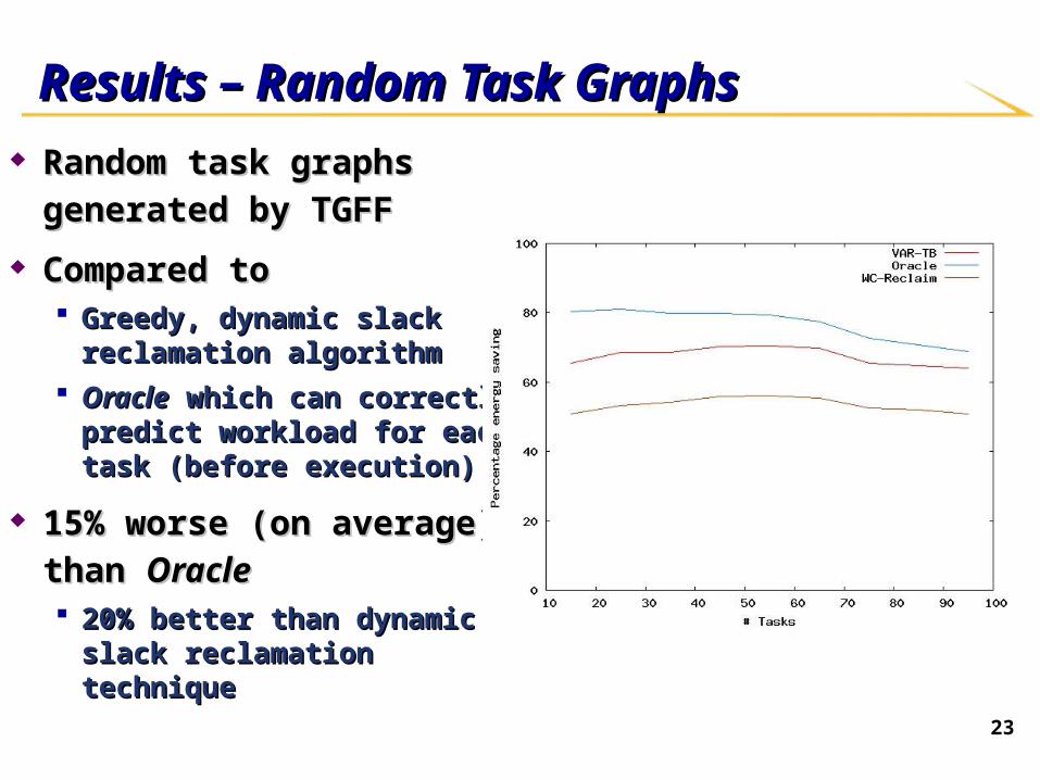
Results – Random Task GraphsResults – Random Task Graphs Random task graphs generated by Random task graphs generated by
TGFFTGFF
Compared toCompared to Greedy, dynamic slack reclamation Greedy, dynamic slack reclamation
algorithmalgorithm
OracleOracle which can correctly predict which can correctly predict workload for each task (before workload for each task (before execution)execution)
15% worse (on average) than 15% worse (on average) than
OracleOracle 20% better than dynamic slack 20% better than dynamic slack
reclamation techniquereclamation technique
24
Real-world ApplicationsReal-world Applications Experimentation methodologyExperimentation methodology
SESC+Wattch for energy of processor cores – 90nmSESC+Wattch for energy of processor cores – 90nm CACTI for cachesCACTI for caches Energy values for ALU, decoder etc obtained by scaling to 180nm Energy values for ALU, decoder etc obtained by scaling to 180nm
values provided by Wattchvalues provided by Wattch CACTI provides energy values for 90nm for SRAM based array CACTI provides energy values for 90nm for SRAM based array
structure in CPUstructure in CPU FIFOs for communication between processorsFIFOs for communication between processors
• Similar to Fast Simplex Links provided by XilinxSimilar to Fast Simplex Links provided by Xilinx
Processors modeled similar to Intel XScaleProcessors modeled similar to Intel XScale 7 voltage levels with speeds varying from 100MHz to 800MHz7 voltage levels with speeds varying from 100MHz to 800MHz
25
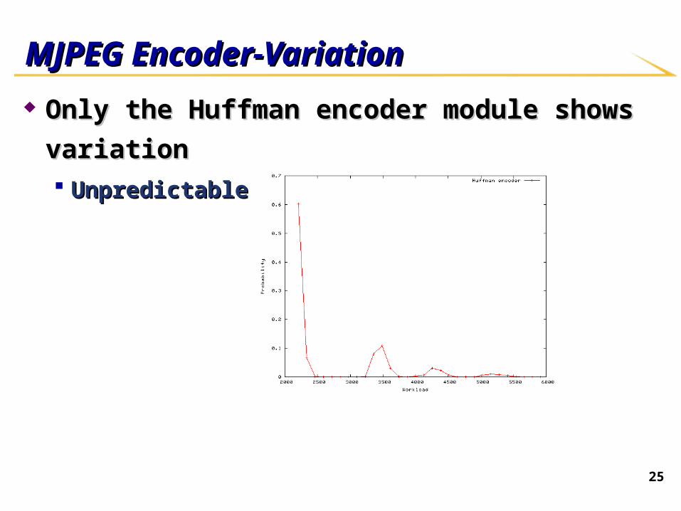
MJPEG Encoder-VariationMJPEG Encoder-Variation
Only the Huffman encoder module shows variationOnly the Huffman encoder module shows variation Unpredictable variationUnpredictable variation
26
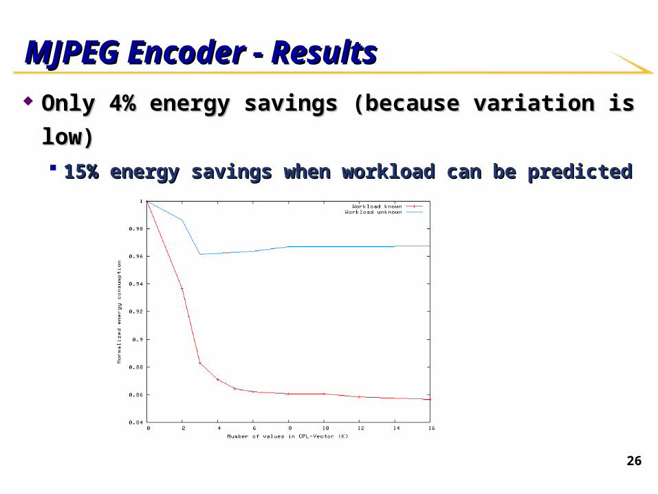
MJPEG Encoder - ResultsMJPEG Encoder - Results
Only 4% energy savings (because variation is low)Only 4% energy savings (because variation is low) 15% energy savings when workload can be predicted15% energy savings when workload can be predicted
27
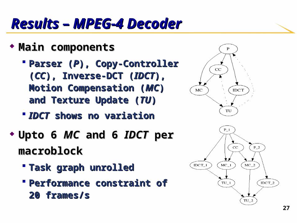
Results – MPEG-4 DecoderResults – MPEG-4 Decoder
Main componentsMain components Parser (Parser (PP), Copy-Controller (), Copy-Controller (CCCC), ),
Inverse-DCT (Inverse-DCT (IDCTIDCT), Motion ), Motion Compensation (Compensation (MCMC) and Texture ) and Texture Update (Update (TUTU))
IDCTIDCT shows no variation shows no variation
Upto 6 Upto 6 MCMC and 6 and 6 IDCTIDCT per per
macroblockmacroblock Task graph unrolledTask graph unrolled
Performance constraint of 20 frames/sPerformance constraint of 20 frames/s

28
MPEG-4 VariationMPEG-4 Variation
CCCC and and MCMC show nice variation show nice variation
(a) (b)

29
MPEG-4 Decoder - ResultsMPEG-4 Decoder - Results Comparison with dynamic slack reclamation algorithmComparison with dynamic slack reclamation algorithm
Upto 20% savings in energy over dynamic slack reclamationUpto 20% savings in energy over dynamic slack reclamation
We measure the effect of the number of values in the schedule tableWe measure the effect of the number of values in the schedule table
30
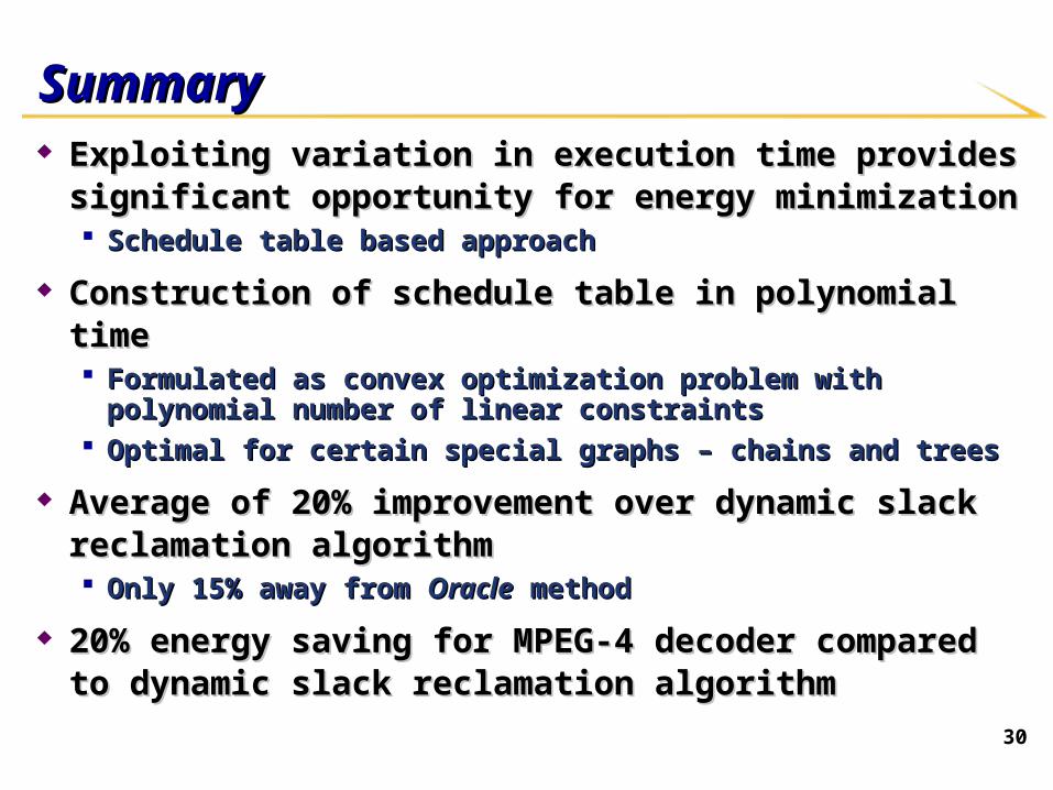
SummarySummary Exploiting variation in execution time provides significant Exploiting variation in execution time provides significant
opportunity for energy minimizationopportunity for energy minimization Schedule table based approachSchedule table based approach
Construction of schedule table in polynomial timeConstruction of schedule table in polynomial time Formulated as convex optimization problem with polynomial number of linear Formulated as convex optimization problem with polynomial number of linear
constraintsconstraints Optimal for certain special graphs – chains and treesOptimal for certain special graphs – chains and trees
Average of 20% improvement over dynamic slack reclamation Average of 20% improvement over dynamic slack reclamation algorithmalgorithm Only 15% away from Only 15% away from OracleOracle method method
20% energy saving for MPEG-4 decoder compared to dynamic slack 20% energy saving for MPEG-4 decoder compared to dynamic slack reclamation algorithmreclamation algorithm

Assuring application-level Assuring application-level correctness against soft errorscorrectness against soft errors
MotivationMotivation
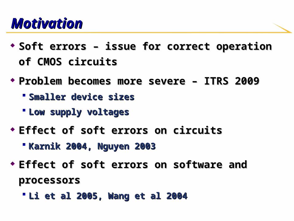
Soft errors – issue for correct operation of CMOS circuitsSoft errors – issue for correct operation of CMOS circuits
Problem becomes more severe – ITRS 2009Problem becomes more severe – ITRS 2009 Smaller device sizesSmaller device sizes
Low supply voltagesLow supply voltages
Effect of soft errors on circuitsEffect of soft errors on circuits Karnik 2004, Nguyen 2003Karnik 2004, Nguyen 2003
Effect of soft errors on software and processorsEffect of soft errors on software and processors Li et al 2005, Wang et al 2004Li et al 2005, Wang et al 2004
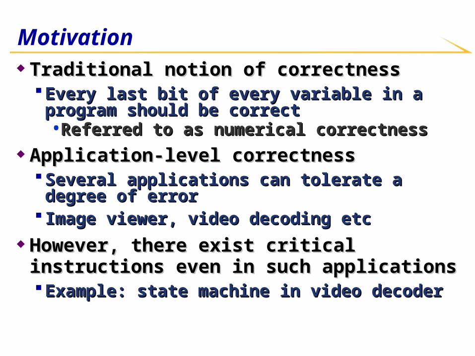
Motivation Traditional notion of correctnessTraditional notion of correctness
Every last bit of every variable in a program should Every last bit of every variable in a program should be correctbe correct• Referred to as numerical correctnessReferred to as numerical correctness
Application-level correctnessApplication-level correctness Several applications can tolerate a degree of errorSeveral applications can tolerate a degree of error Image viewer, video decoding etcImage viewer, video decoding etc
However, there exist critical instructions even in However, there exist critical instructions even in such applicationssuch applications Example: state machine in video decoderExample: state machine in video decoder

MotivationMotivation
Goal: Detect all “critical” instructions in the programGoal: Detect all “critical” instructions in the program
Protect “critical” instructions in the program against soft Protect “critical” instructions in the program against soft
errorserrors Using duplicationUsing duplication
OutlineOutline
MotivationMotivation
Definition of critical instructionsDefinition of critical instructions
Program representationProgram representation
Static analysis to detect critical instructionsStatic analysis to detect critical instructions
Profiling and runtime monitoringProfiling and runtime monitoring
ResultsResults
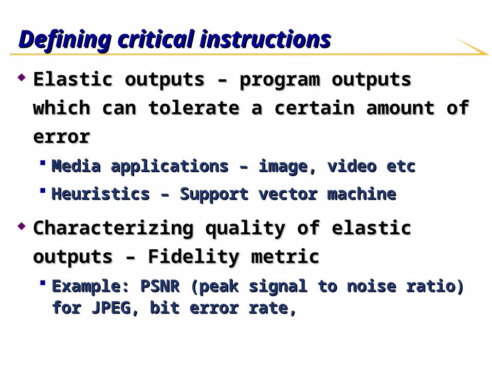
Defining critical instructionsDefining critical instructions
Elastic outputs – program outputs which can tolerate a Elastic outputs – program outputs which can tolerate a
certain amount of errorcertain amount of error Media applications – image, video etcMedia applications – image, video etc
Heuristics – Support vector machineHeuristics – Support vector machine
Characterizing quality of elastic outputs – Fidelity metricCharacterizing quality of elastic outputs – Fidelity metric Example: PSNR (peak signal to noise ratio) for JPEG, bit error Example: PSNR (peak signal to noise ratio) for JPEG, bit error
rate, rate,
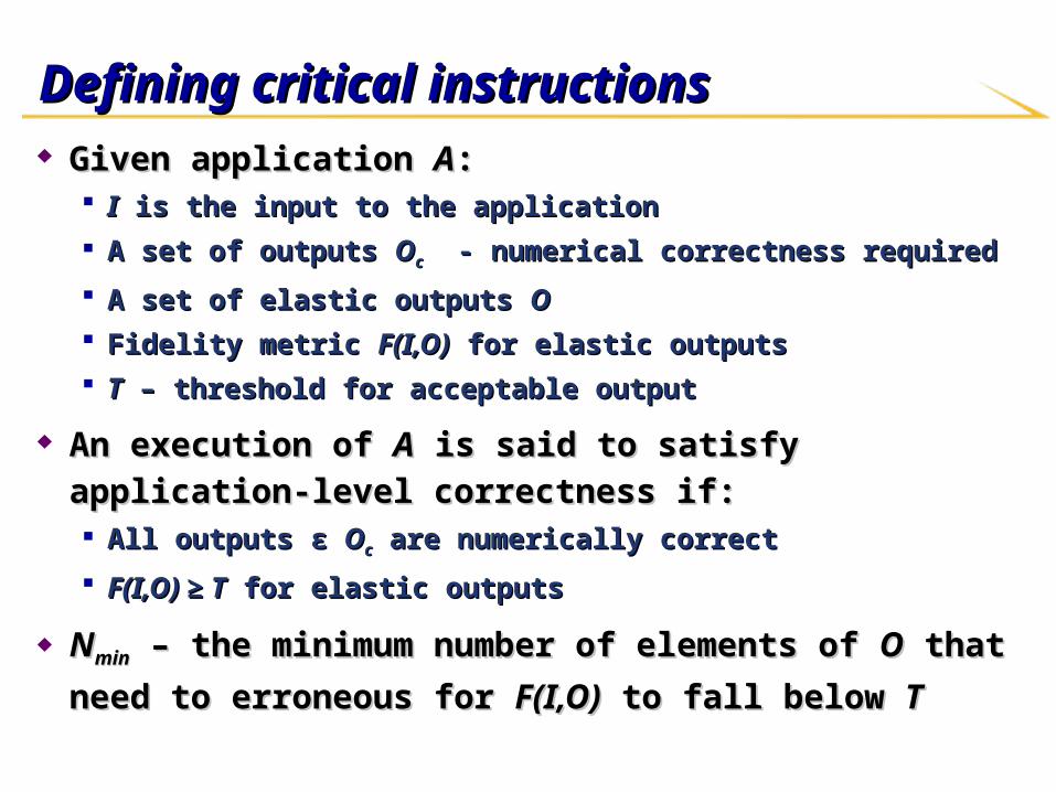
Defining critical instructionsDefining critical instructions Given application Given application AA::
II is the input to the application is the input to the application
A set of outputs A set of outputs OOcc - numerical correctness required - numerical correctness required
A set of elastic outputs A set of elastic outputs OO
Fidelity metric Fidelity metric F(I,O)F(I,O) for elastic outputs for elastic outputs
TT – threshold for acceptable output – threshold for acceptable output
An execution of An execution of AA is said to satisfy application-level correctness if: is said to satisfy application-level correctness if: All outputs All outputs εε OOcc are numerically correct are numerically correct
F(I,O) ≥ TF(I,O) ≥ T for elastic outputs for elastic outputs
NNminmin – the minimum number of elements of – the minimum number of elements of OO that need to erroneous that need to erroneous
for for F(I,O)F(I,O) to fall below to fall below TT
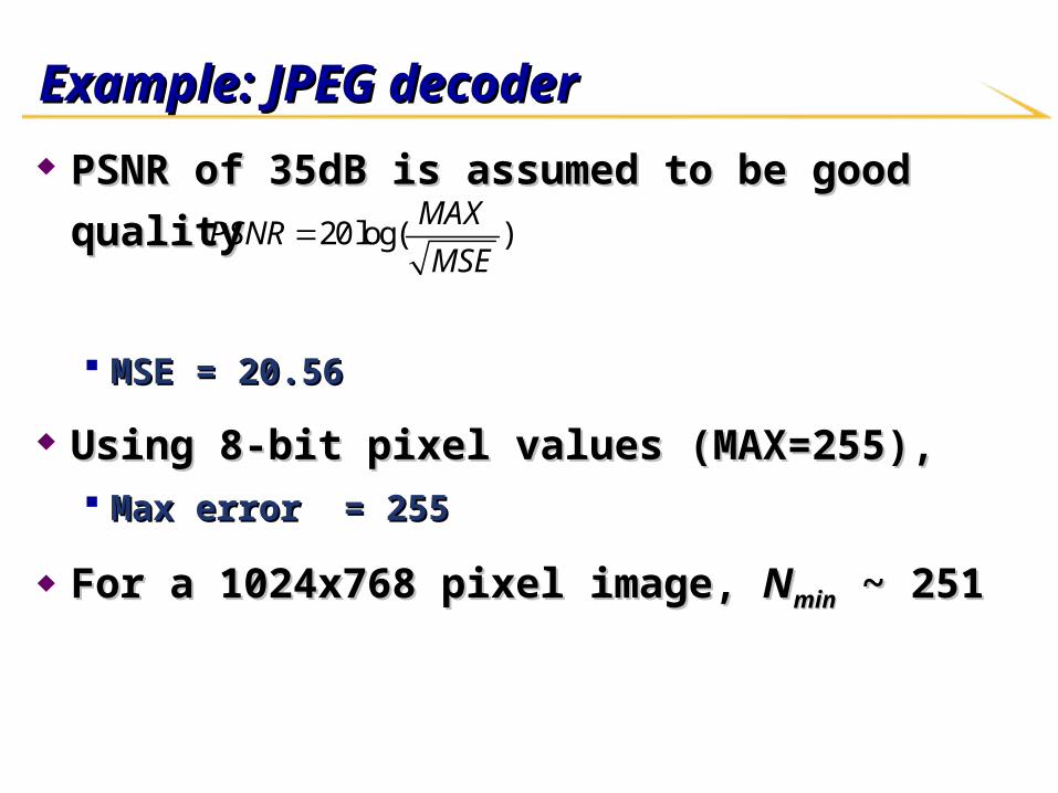
Example: JPEG decoderExample: JPEG decoder
PSNR of 35dB is assumed to be good qualityPSNR of 35dB is assumed to be good quality
MSE = 20.56MSE = 20.56
Using 8-bit pixel values (MAX=255), Using 8-bit pixel values (MAX=255), Max error = 255Max error = 255
For a 1024x768 pixel image, For a 1024x768 pixel image, NNminmin ~ 251 ~ 251
20log( )MAX
PSNRMSE

Defining critical instructionsDefining critical instructions
An instruction An instruction XX is said to be critical if is said to be critical if
X affects one of the outputs of X affects one of the outputs of OOcc (numerical correctness (numerical correctness
required) ORrequired) OR
X affects X affects NNminmin elastic output elements elastic output elements OO

OutlineOutline
MotivationMotivation
Definition of critical instructionsDefinition of critical instructions
Program representationProgram representation
Static analysis to detect critical instructionsStatic analysis to detect critical instructions
Profiling and runtime monitoringProfiling and runtime monitoring
ResultsResults

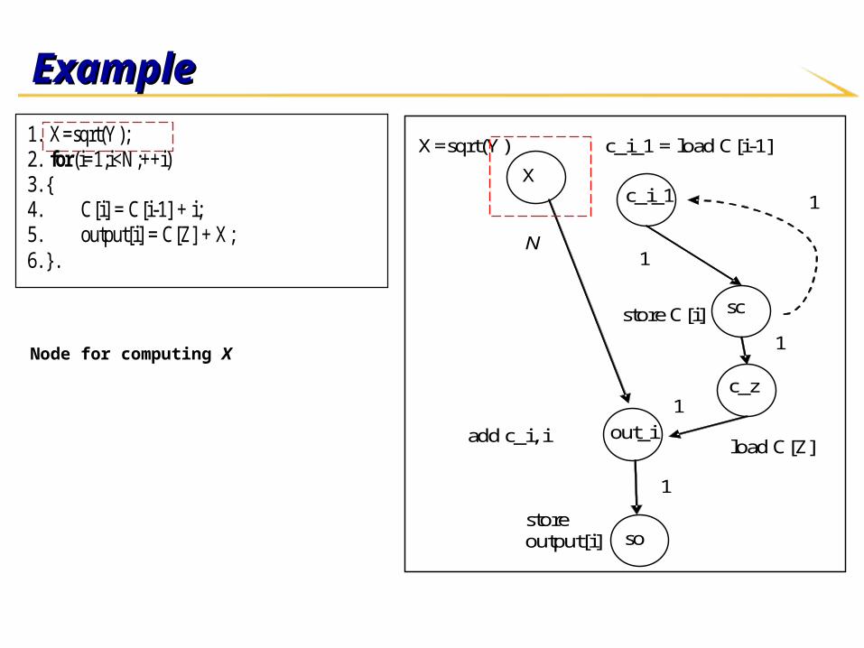
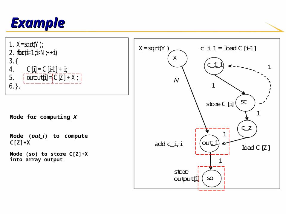
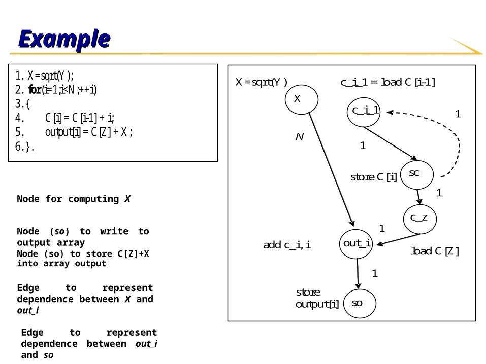
Program representationProgram representation
LLVM compiler infrastructureLLVM compiler infrastructure LLVM intermediate representationLLVM intermediate representation
Weighted program dependence graph (PDG) – Weighted program dependence graph (PDG) – GG

ExampleExample
1. X=sqrt(Y); 2. for(i=1;i<N;++i) 3. { 4. C[i] = C[i-1] + i; 5. output[i] = C[Z] + X; 6. }.
1. X=sqrt(Y); 2. bb: 3. i = phi([0,entry], [i_next, bb]); 4. c_i_1 = load &C[i-1] 5. tmp = add c_i_1, i 6. store c_1_1, &C[i] 7. c_z = load &C[Z] 8. out_i = add X, c_i 9. store out_i &output[i]
LLVM IR – 3 address code
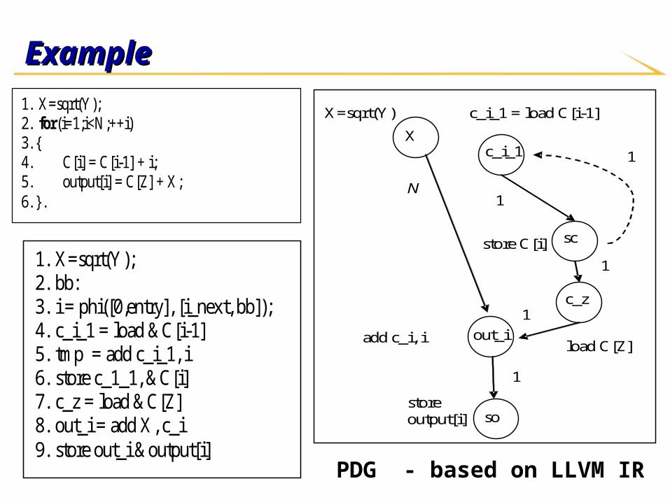
ExampleExample
1. X=sqrt(Y); 2. for(i=1;i<N;++i) 3. { 4. C[i] = C[i-1] + i; 5. output[i] = C[Z] + X; 6. }.
add c_i, i load C[Z]
c_i_1 = load C[i-1]
c_i_1
sc
c_z
out_i
store C[i]
1
1
1
1
X
N
X=sqrt(Y)
store output[i] so
1
1. X=sqrt(Y); 2. bb: 3. i = phi([0,entry], [i_next, bb]); 4. c_i_1 = load &C[i-1] 5. tmp = add c_i_1, i 6. store c_1_1, &C[i] 7. c_z = load &C[Z] 8. out_i = add X, c_i 9. store out_i &output[i]
PDG - based on LLVM IR
ExampleExample
1. X=sqrt(Y); 2. for(i=1;i<N;++i) 3. { 4. C[i] = C[i-1] + i; 5. output[i] = C[Z] + X; 6. }.
add c_i, i load C[Z]
c_i_1 = load C[i-1]
c_i_1
sc
c_z
out_i
store C[i]
1
1
1
1
X
N
X=sqrt(Y)
store output[i] so
1
Node for computing X
ExampleExample
1. X=sqrt(Y); 2. for(i=1;i<N;++i) 3. { 4. C[i] = C[i-1] + i; 5. output[i] = C[Z] + X; 6. }.
add c_i, i load C[Z]
c_i_1 = load C[i-1]
c_i_1
sc
c_z
out_i
store C[i]
1
1
1
1
X
N
X=sqrt(Y)
store output[i] so
1
Node for computing X
Node (out_i) to compute C[Z]+X
Node (so) to store C[Z]+X into array output
ExampleExample
1. X=sqrt(Y); 2. for(i=1;i<N;++i) 3. { 4. C[i] = C[i-1] + i; 5. output[i] = C[Z] + X; 6. }.
add c_i, i load C[Z]
c_i_1 = load C[i-1]
c_i_1
sc
c_z
out_i
store C[i]
1
1
1
1
X
N
X=sqrt(Y)
store output[i] so
1
Node for computing X
Node (so) to write to output array
Edge to represent dependence between X and out_i
Node (so) to store C[Z]+X into array output
Edge to represent dependence between out_i and so
Assigning edge weightsAssigning edge weights Edge weight Edge weight u→v u→v - how many - how many
instances of node v are affected instances of node v are affected
by 1 instance of by 1 instance of uu??
Example:Example:
XX outside the loop, outside the loop, out_iout_i inside inside
the loopthe loop Edge weight NEdge weight N
Nodes Nodes out_iout_i and and soso are in the are in the
same basic block – same basic block – Edge weight 1Edge weight 1
add c_i, i load C[Z]
c_i_1 = load C[i-1]
c_i_1
sc
c_z
out_i
store C[i]
1
1
1
1
X
N
X=sqrt(Y)
store output[i] so
1
OutlineOutline
MotivationMotivation
Definition of critical instructionsDefinition of critical instructions
Program representationProgram representation
Static analysis to detect critical instructionsStatic analysis to detect critical instructions
Profiling and runtime monitoringProfiling and runtime monitoring
ResultsResults
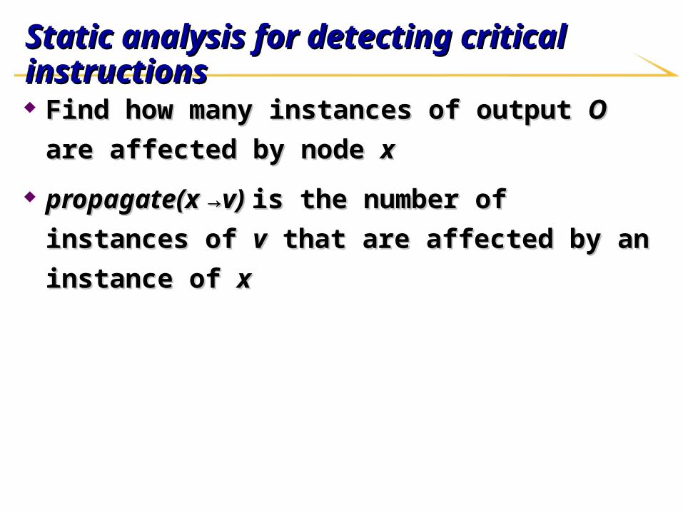
Static analysis for detecting critical Static analysis for detecting critical instructionsinstructions Find how many instances of output Find how many instances of output OO are affected by node are affected by node
xx
propagate(x →v) propagate(x →v) is the number of instances of is the number of instances of vv that are that are
affected by an instance of affected by an instance of xx

ExampleExample propagate(u→v)propagate(u→v) initialized to edge weight for initialized to edge weight for
all edges all edges (u →v)(u →v)
propagate(X →out_i) = Npropagate(X →out_i) = N
w(out_i →so) = 1w(out_i →so) = 1
propagate(X →so) = propagate(X →out_i) *propagate(X →so) = propagate(X →out_i) *
w(out_i →so)w(out_i →so)
More formallyMore formally
add c_i, i load C[Z]
c_i_1 = load C[i-1]
c_i_1
sc
c_z
out_i
store C[i]
1
1
1
1
X
N
X=sqrt(Y)
store output[i] so
1
( )( ) max ( ( )* ( ))
u predecessors vpropagate x v propagate x u w u v
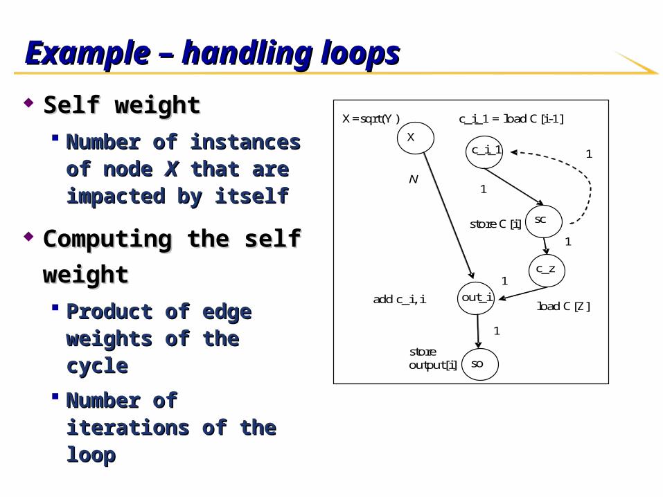
Example – handling loops Example – handling loops
Self weightSelf weight Number of instances of Number of instances of
node node XX that are impacted that are impacted by itselfby itself
Computing the self Computing the self
weightweight Product of edge weights Product of edge weights
of the cycleof the cycle
Number of iterations of the Number of iterations of the looploop
add c_i, i load C[Z]
c_i_1 = load C[i-1]
c_i_1
sc
c_z
out_i
store C[i]
1
1
1
1
X
N
X=sqrt(Y)
store output[i] so
1
OutlineOutline
MotivationMotivation
Definition of critical instructionsDefinition of critical instructions
Program representationProgram representation
Static analysis to detect critical instructionsStatic analysis to detect critical instructions
Profiling and runtime monitoringProfiling and runtime monitoring
ResultsResults

Profiling and runtime monitoringProfiling and runtime monitoring
Static analysis is conservative in natureStatic analysis is conservative in nature May produce overly pessimistic resultsMay produce overly pessimistic results
Main reason – edge weights are initialized too highMain reason – edge weights are initialized too high
Profiling with test inputs to estimate edge weightsProfiling with test inputs to estimate edge weights
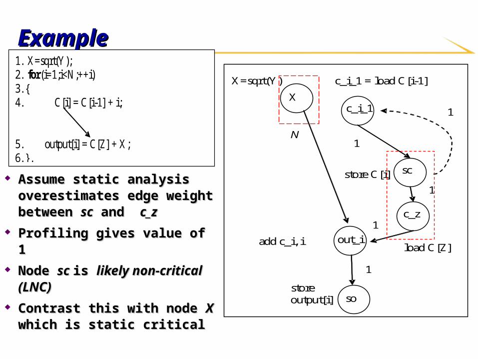
ExampleExample
Assume static analysis Assume static analysis overestimates edge weight overestimates edge weight between between scsc and and c_zc_z
Profiling gives value of 1Profiling gives value of 1 Node Node sc sc is is likely non-critical likely non-critical
(LNC)(LNC) Contrast this with node Contrast this with node XX which which
is static criticalis static critical
1. X=sqrt(Y); 2. for(i=1;i<N;++i) 3. { 4. C[i] = C[i-1] + i; 5. output[i] = C[Z] + X; 6. }.
add c_i, i load C[Z]
c_i_1 = load C[i-1]
c_i_1
sc
c_z
out_i
store C[i]
1
1
1
1
X
N
X=sqrt(Y)
store output[i] so
1
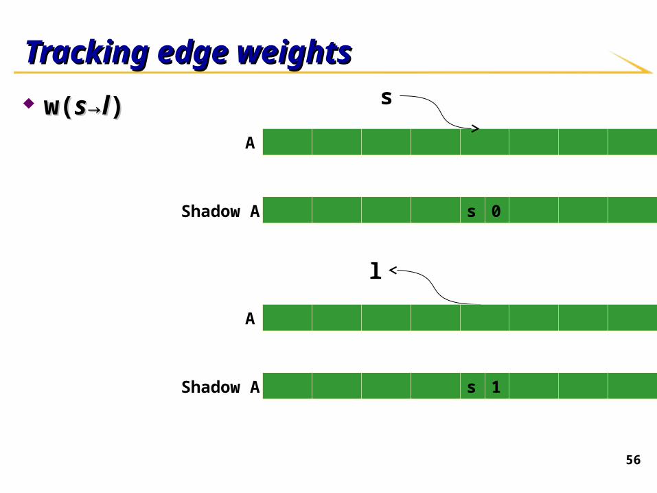
Tracking edge weightsTracking edge weights
w(w(ss→→ll))
56
A
l
s 0Shadow A
A
s 1Shadow A
s
Profiling and runtime monitoringProfiling and runtime monitoring
Likely critical instructions – duplicated and checked in Likely critical instructions – duplicated and checked in
softwaresoftware Using the SWIFT method proposed by Reis et al 2005Using the SWIFT method proposed by Reis et al 2005
Likely non-critical instructions – monitored using Likely non-critical instructions – monitored using
lightweight runtime monitoring techniquelightweight runtime monitoring technique
Static non-critical instructions – no error checkingStatic non-critical instructions – no error checking
OutlineOutline
MotivationMotivation
Definition of critical instructionsDefinition of critical instructions
Program representationProgram representation
Static analysis to detect critical instructionsStatic analysis to detect critical instructions
Profiling and runtime monitoringProfiling and runtime monitoring
ResultsResults
ResultsResults
Benchmarks for Mediabench, SPEC, MibenchBenchmarks for Mediabench, SPEC, Mibench
Simics/GEMS simulation infrastructureSimics/GEMS simulation infrastructure
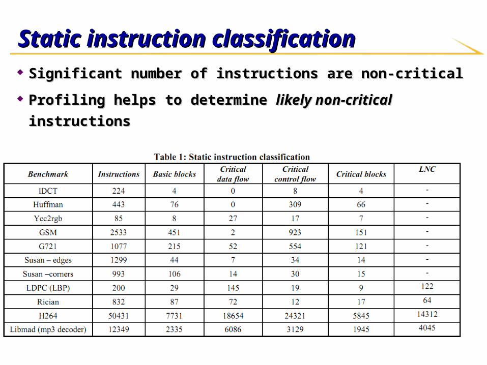
Static instruction classificationStatic instruction classification
Significant number of instructions are non-criticalSignificant number of instructions are non-critical
Profiling helps to determine Profiling helps to determine likely non-criticallikely non-critical instructions instructions
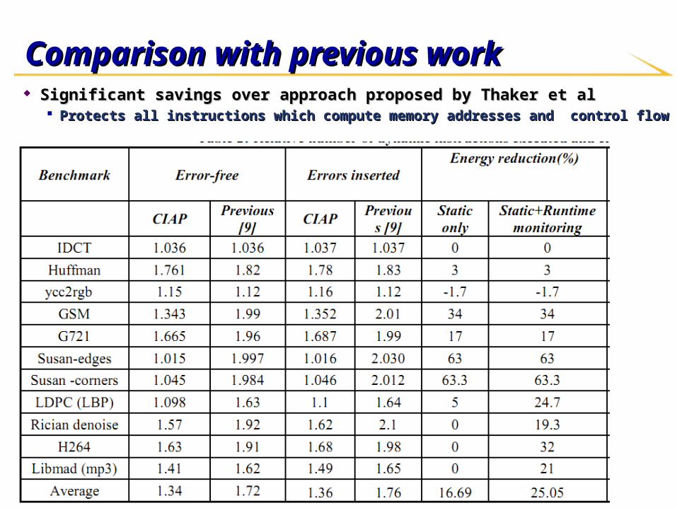
Comparison with previous workComparison with previous work Significant savings over approach proposed by Thaker et alSignificant savings over approach proposed by Thaker et al
Protects all instructions which compute memory addresses and control flowProtects all instructions which compute memory addresses and control flow

ConclusionConclusion
Static + dynamic technique for detecting critical Static + dynamic technique for detecting critical
instructionsinstructions
Detect several non-critical instructionsDetect several non-critical instructions
Reduce overall energy by 25%Reduce overall energy by 25%

Fine grained accelerator integration using 3DFine grained accelerator integration using 3D

Accelerators v/s softwareAccelerators v/s software Accelerators v/s software (Hameed et al ISCA 2010)Accelerators v/s software (Hameed et al ISCA 2010)
Pros: Energy and performance efficiencyPros: Energy and performance efficiency Application specific datapathsApplication specific datapaths
• Customized functional unitsCustomized functional units
ParallelismParallelism• Data parallel and pipelineData parallel and pipeline
Cons:Cons: High design, verification and manufacturing costHigh design, verification and manufacturing cost Reconfigurable systems – still design and verification costReconfigurable systems – still design and verification cost
Customized instructionsCustomized instructions Processor + fine-grained acceleratorProcessor + fine-grained accelerator
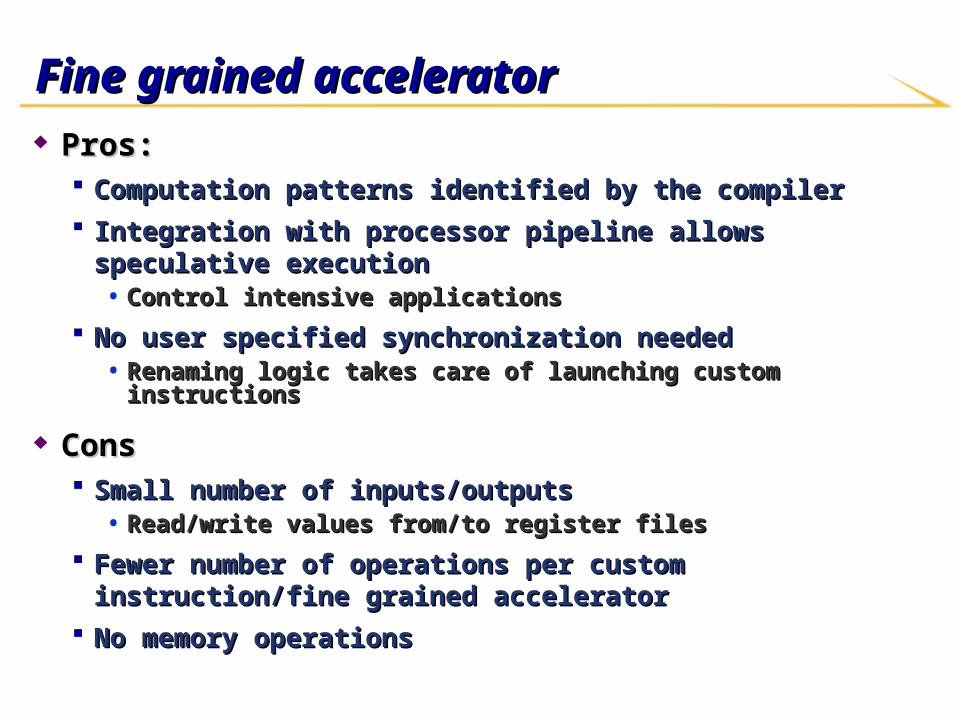
Fine grained acceleratorFine grained accelerator Pros:Pros:
Computation patterns identified by the compilerComputation patterns identified by the compiler Integration with processor pipeline allows speculative executionIntegration with processor pipeline allows speculative execution
• Control intensive applicationsControl intensive applications
No user specified synchronization neededNo user specified synchronization needed• Renaming logic takes care of launching custom instructionsRenaming logic takes care of launching custom instructions
ConsCons Small number of inputs/outputsSmall number of inputs/outputs
• Read/write values from/to register filesRead/write values from/to register files
Fewer number of operations per custom instruction/fine grained Fewer number of operations per custom instruction/fine grained acceleratoraccelerator
No memory operationsNo memory operations
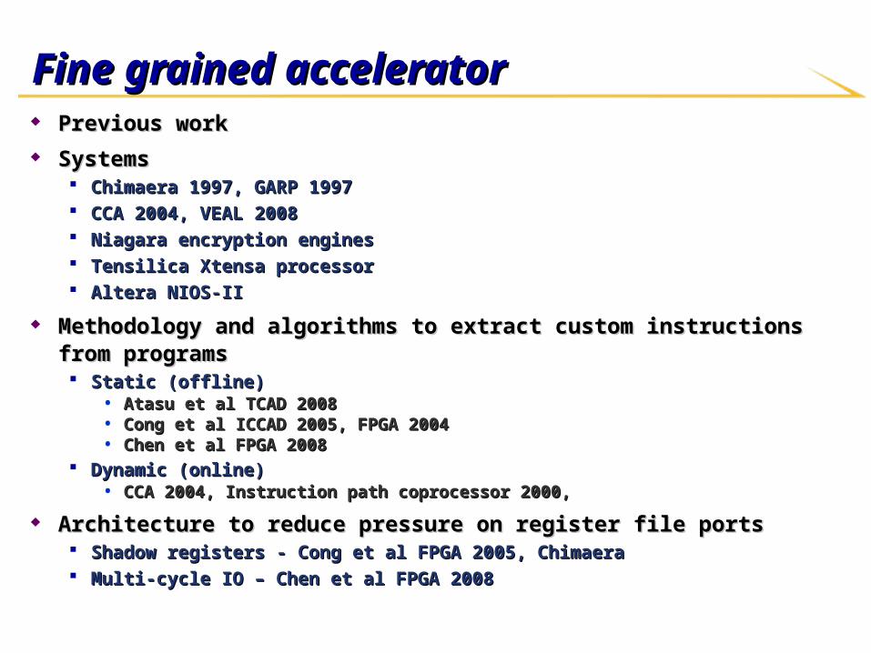
Fine grained acceleratorFine grained accelerator Previous workPrevious work SystemsSystems
Chimaera 1997, GARP 1997Chimaera 1997, GARP 1997 CCA 2004, VEAL 2008CCA 2004, VEAL 2008 Niagara encryption enginesNiagara encryption engines Tensilica Xtensa processorTensilica Xtensa processor Altera NIOS-IIAltera NIOS-II
Methodology and algorithms to extract custom instructions from programsMethodology and algorithms to extract custom instructions from programs Static (offline)Static (offline)
• Atasu et al TCAD 2008Atasu et al TCAD 2008• Cong et al ICCAD 2005, FPGA 2004Cong et al ICCAD 2005, FPGA 2004• Chen et al FPGA 2008Chen et al FPGA 2008
Dynamic (online)Dynamic (online)• CCA 2004, Instruction path coprocessor 2000, CCA 2004, Instruction path coprocessor 2000,
Architecture to reduce pressure on register file portsArchitecture to reduce pressure on register file ports Shadow registers - Cong et al FPGA 2005, ChimaeraShadow registers - Cong et al FPGA 2005, Chimaera Multi-cycle IO – Chen et al FPGA 2008Multi-cycle IO – Chen et al FPGA 2008
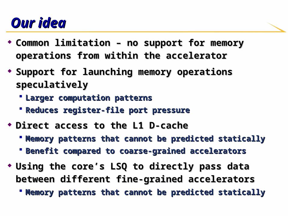
Our ideaOur idea Common limitation – no support for memory operations from Common limitation – no support for memory operations from
within the acceleratorwithin the accelerator
Support for launching memory operations speculativelySupport for launching memory operations speculatively Larger computation patternsLarger computation patterns Reduces register-file port pressureReduces register-file port pressure
Direct access to the L1 D-cacheDirect access to the L1 D-cache Memory patterns that cannot be predicted staticallyMemory patterns that cannot be predicted statically Benefit compared to coarse-grained acceleratorsBenefit compared to coarse-grained accelerators
Using the core’s LSQ to directly pass data between different Using the core’s LSQ to directly pass data between different
fine-grained acceleratorsfine-grained accelerators Memory patterns that cannot be predicted staticallyMemory patterns that cannot be predicted statically

ExampleExample
1. for(i = 1 to N) { 2. C[i] = A[i] – X * Y; 3. A[Z] = B[i] + X * Y; 4. }
load B[i]
*
+
Store A[Z]
load A[i]
−
Store C[i]
XY
*
X Y
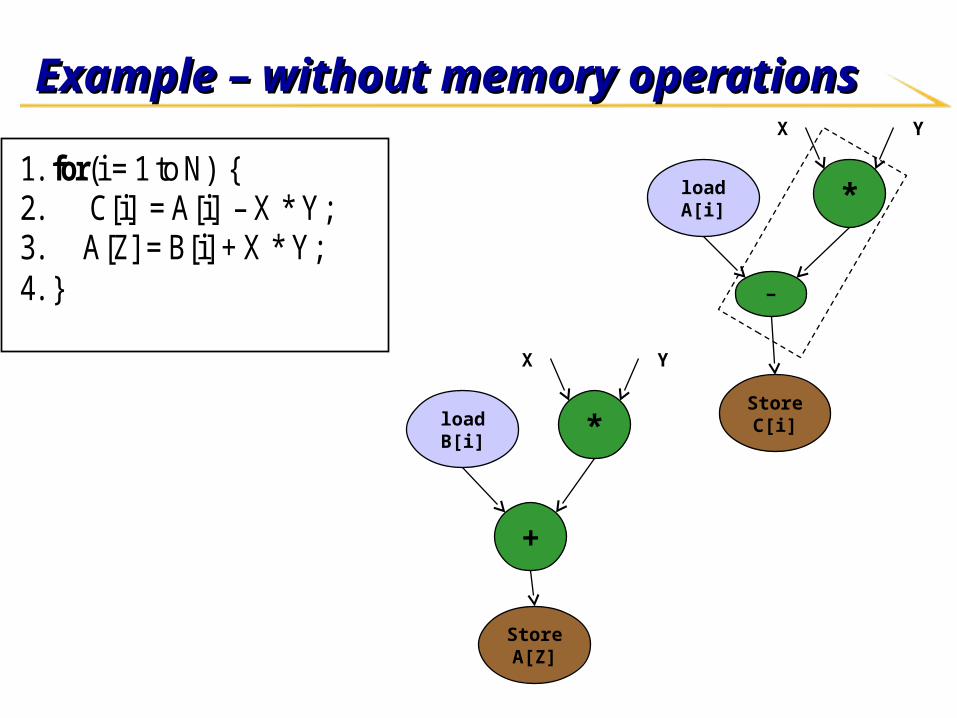
Example – without memory operationsExample – without memory operations
load B[i]
*
+
Store A[Z]
load A[i]
−
Store C[i]
X Y
*
X Y
1. for(i = 1 to N) { 2. C[i] = A[i] – X * Y; 3. A[Z] = B[i] + X * Y; 4. }
Example – with memory operationsExample – with memory operations
1. for(i = 1 to N) { 2. C[i] = A[i] – X * Y; 3. A[Z] = B[i] + X * Y; 4. }
load B[i]
*
+
Store A[Z]
X Y
load A[i]
−
Store C[i]
*
X Y
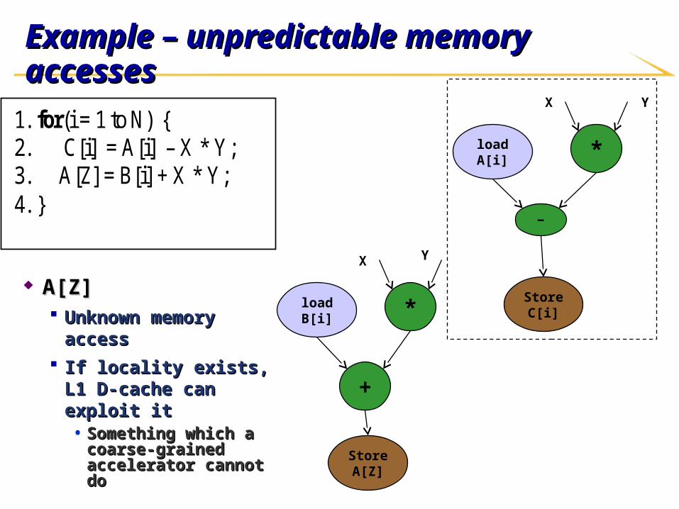
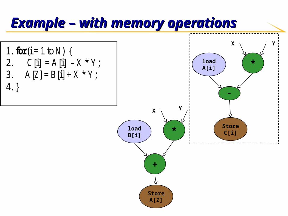
Example – unpredictable memory accessesExample – unpredictable memory accesses
A[Z]A[Z] Unknown memory Unknown memory
accessaccess If locality exists, L1 D-If locality exists, L1 D-
cache can exploit itcache can exploit it• Something which a Something which a
coarse-grained coarse-grained accelerator cannot doaccelerator cannot do
1. for(i = 1 to N) { 2. C[i] = A[i] – X * Y; 3. A[Z] = B[i] + X * Y; 4. }
load B[i]
*
+
Store A[Z]
X Y
load A[i]
−
Store C[i]
*
X Y
Example – speculative pipeliningExample – speculative pipelining
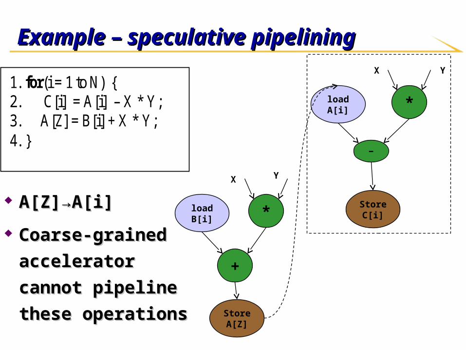
A[Z]→A[i]A[Z]→A[i]
Coarse-grained Coarse-grained
accelerator cannot accelerator cannot
pipeline these pipeline these
operationsoperations
1. for(i = 1 to N) { 2. C[i] = A[i] – X * Y; 3. A[Z] = B[i] + X * Y; 4. }
load B[i]
*
+
Store A[Z]
X Y
load A[i]
−
Store C[i]
*
X Y

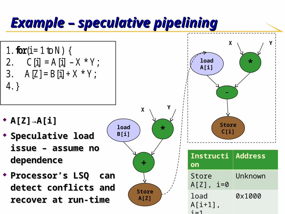
Example – speculative pipeliningExample – speculative pipelining
A[Z]→A[i]A[Z]→A[i]
Speculative load issue – Speculative load issue –
assume no dependenceassume no dependence
Processor’s LSQ can Processor’s LSQ can
detect conflicts and detect conflicts and
recover at run-timerecover at run-time
1. for(i = 1 to N) { 2. C[i] = A[i] – X * Y; 3. A[Z] = B[i] + X * Y; 4. }
load B[i]
*
+
Store A[Z]
X Y
load A[i]
−
Store C[i]
*
X Y
Instruction Address
Store A[Z], i=0 Unknown
load A[i+1], i=1 0x1000

Example – speculative pipeliningExample – speculative pipelining
A[Z]→A[i]A[Z]→A[i]
Speculative load issue – Speculative load issue –
assume no dependenceassume no dependence
Processor’s LSQ can Processor’s LSQ can
detect conflicts and detect conflicts and
recover at run-timerecover at run-time
1. for(i = 1 to N) { 2. C[i] = A[i] – X * Y; 3. A[Z] = B[i] + X * Y; 4. }
load B[i]
*
+
Store A[Z]
X Y
load A[i]
−
Store C[i]
*
X Y
Instruction Address
Store A[Z], i=0 0x1000
load A[i+1], i=1 0x1000
CONFLICT
Fine-grained accelerators – constraintsFine-grained accelerators – constraints
Custom instructionsCustom instructions No special operations allowed inside custom instructionNo special operations allowed inside custom instruction
• Function call, atomics, volatile writes/reads etcFunction call, atomics, volatile writes/reads etc
Primary inputs from register filesPrimary inputs from register files• All registers need to be ready before the custom instruction is All registers need to be ready before the custom instruction is
launchedlaunched• Restricts the number of input/outputsRestricts the number of input/outputs
Can launch read/write memory operationsCan launch read/write memory operations• Number of memory operations must be known given the custom Number of memory operations must be known given the custom
instructioninstruction
No internal dependences/state within a custom instructionNo internal dependences/state within a custom instruction• For identical inputs, produces identical outputsFor identical inputs, produces identical outputs
Example – constraints on memory operationsExample – constraints on memory operations
A[Z]→A[i] possible A[Z]→A[i] possible
dependencedependence
Clustering would cause Clustering would cause
dependence within an dependence within an
instructioninstruction
1. for(i = 1 to N) { 2. A[Z] = B[i] + X * Y; 3. C[i] = A[i] – X * Y; 4. }
load B[i]
*
+
Store A[Z]
X Y
load A[i]
−
Store C[i]
*
X Y
Fine-grained accelerators – constraintsFine-grained accelerators – constraints
Memory operationsMemory operations No store-load aliased pair within a custom instructionNo store-load aliased pair within a custom instruction
Easy ordering of memory operationsEasy ordering of memory operations All load operations are launched at the beginning of the custom All load operations are launched at the beginning of the custom
instructioninstruction
All store operations are launched at the end of the custom All store operations are launched at the end of the custom instructioninstruction
ArchitectureArchitecture Decode stageDecode stage
Register renamingRegister renaming• X, Y, i, B, A, ZX, Y, i, B, A, Z
Number of memory operations to Number of memory operations to launch (launch (NN))
• Provided by CFU memop tableProvided by CFU memop table• SRAM arraySRAM array• # entries = # custom instructions# entries = # custom instructions
Example: N=2Example: N=2
Decode
Dispatch
Reservation station
ALU CFUMemory
unit
ROB
CFU memop table
load B[i] *
+
Store
A[Z]
X Y
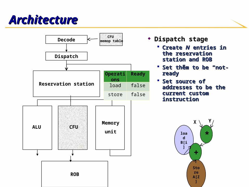
ArchitectureArchitecture
Dispatch stageDispatch stage Create Create NN entries in the entries in the
reservation station and ROBreservation station and ROB Set them to be “not-ready”Set them to be “not-ready” Set source of addresses to Set source of addresses to
be the current custom be the current custom instructioninstruction
Decode
Dispatch
Reservation station
ALU CFUMemory
unit
ROB
CFU memop table
load B[i] *
+
Store
A[Z]
X Y
Operations Ready
load false
store false

ArchitectureArchitecture
Execute stageExecute stage CFU computes addresses CFU computes addresses
for memory operationsfor memory operations
Sends them over bypass Sends them over bypass paths to reservation paths to reservation stationstation
Decode
Dispatch
Reservation station
ALU CFUMemory
unit
ROB
CFU memop table
Operations Ready
load true
store false
load B[i] *
+
Store
A[Z]
X Y
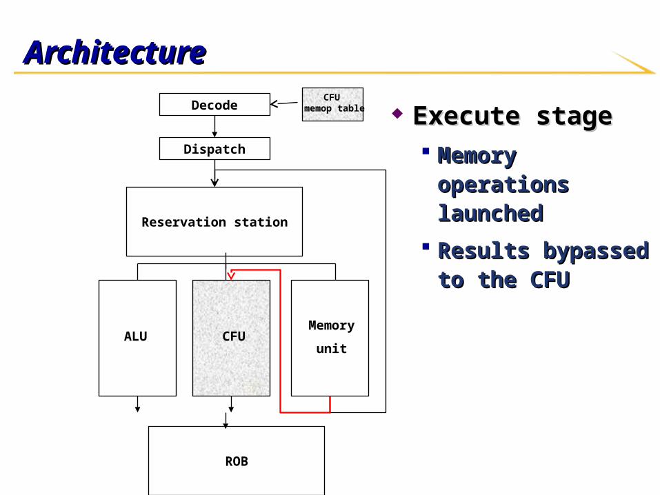
ArchitectureArchitecture
Execute stageExecute stage Memory operations Memory operations
launchedlaunched
Results bypassed to the Results bypassed to the CFUCFU
Decode
Dispatch
Reservation station
ALU CFUMemory
unit
ROB
CFU memop table
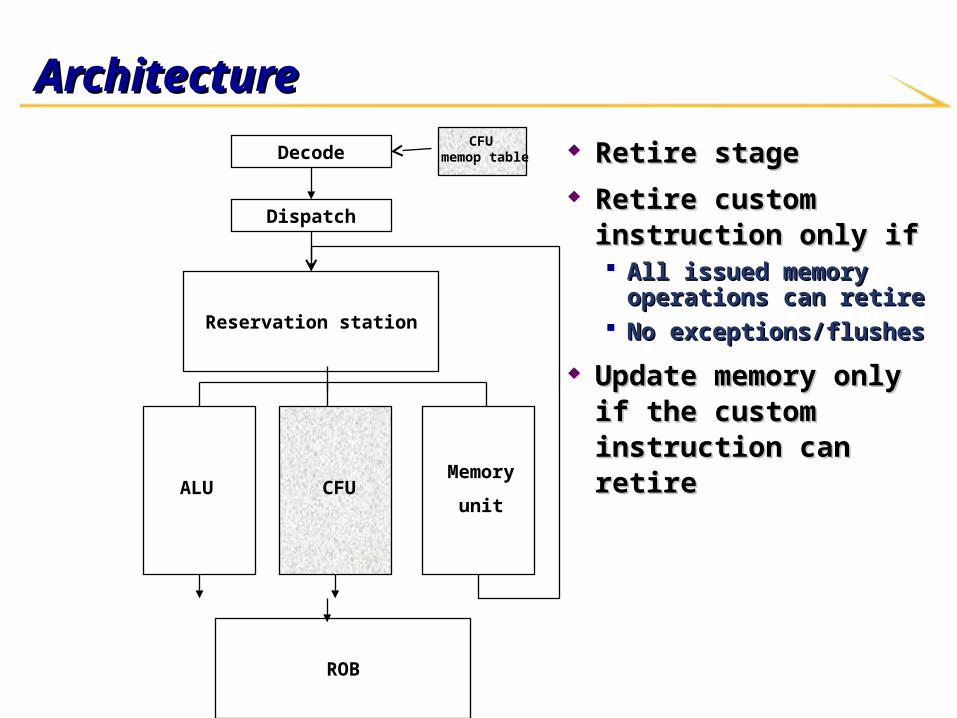
ArchitectureArchitecture
Retire stageRetire stage Retire custom instruction Retire custom instruction
only ifonly if All issued memory operations All issued memory operations
can retirecan retire No exceptions/flushes No exceptions/flushes
Update memory only if the Update memory only if the custom instruction can custom instruction can retireretire
Decode
Dispatch
Reservation station
ALU CFUMemory
unit
ROB
CFU memop table
Architecture – ids for forwarding dataArchitecture – ids for forwarding data Register renaming – id of the physical register is sent over Register renaming – id of the physical register is sent over
the bypass pathsthe bypass paths No physical register for memory operations launched by the No physical register for memory operations launched by the
custom instructioncustom instruction
Id of the custom instruction/memory operation usedId of the custom instruction/memory operation used ROB entry idROB entry id
Assuming Assuming 256 entries in physical register file256 entries in physical register file
256 entries in ROB256 entries in ROB
Total 512 different ids possibleTotal 512 different ids possible• Id 8 bit → 9 bitId 8 bit → 9 bit
Using 3DUsing 3D
Why?Why? Different vendors, different technology nodesDifferent vendors, different technology nodes
More reconfigurable fabric per core available for More reconfigurable fabric per core available for
Custom instructionsCustom instructions Communication using TSVsCommunication using TSVs
Area overheadArea overhead Requirement - 2048 TSVs per core for a 4-issue superscalar Requirement - 2048 TSVs per core for a 4-issue superscalar
processorprocessor
Area – 0.2048 mmArea – 0.2048 mm22 assuming 10 assuming 10μμm TSV pitch (IMEC 2008)m TSV pitch (IMEC 2008) Small compared to area of processor core (7mmSmall compared to area of processor core (7mm22))
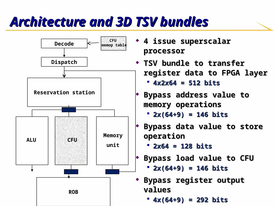
Architecture and 3D TSV bundlesArchitecture and 3D TSV bundles 4 issue superscalar processor4 issue superscalar processor TSV bundle to transfer register data to TSV bundle to transfer register data to
FPGA layerFPGA layer 4x2x64 = 512 bits4x2x64 = 512 bits
Bypass address value to memory Bypass address value to memory operationsoperations 2x(64+9) = 146 bits2x(64+9) = 146 bits
Bypass data value to store operationBypass data value to store operation 2x64 = 128 bits2x64 = 128 bits
Bypass load value to CFUBypass load value to CFU 2x(64+9) = 146 bits2x(64+9) = 146 bits
Bypass register output values Bypass register output values 4x(64+9) = 292 bits4x(64+9) = 292 bits
Decode
Dispatch
Reservation station
ALU CFUMemory
unit
ROB
CFU memop table

Compilation flowCompilation flow
LLVM compilation frameworkLLVM compilation framework
Common constraintsCommon constraints Convex data flowConvex data flow
No special instructions inside custom instructionNo special instructions inside custom instruction
Control flow can span multiple blocksControl flow can span multiple blocks No loops within a single custom instructionNo loops within a single custom instruction
Single entry, multiple exitsSingle entry, multiple exits
MemoryMemory No memory dependence within a custom instructionNo memory dependence within a custom instruction
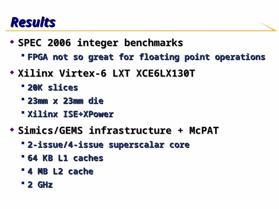
ResultsResults SPEC 2006 integer benchmarksSPEC 2006 integer benchmarks
FPGA not so great for floating point operationsFPGA not so great for floating point operations
Xilinx Virtex-6 LXT XCE6LX130T Xilinx Virtex-6 LXT XCE6LX130T 20K slices20K slices 23mm x 23mm die23mm x 23mm die Xilinx ISE+XPowerXilinx ISE+XPower
Simics/GEMS infrastructure + McPATSimics/GEMS infrastructure + McPAT 2-issue/4-issue superscalar core2-issue/4-issue superscalar core 64 KB L1 caches64 KB L1 caches 4 MB L2 cache4 MB L2 cache 2 GHz2 GHz

Choosing custom instructionsChoosing custom instructions Profiling: identify 10 hottest loops of Profiling: identify 10 hottest loops of
each programeach program
Sort basic blocks in each loop in Sort basic blocks in each loop in
topological ordertopological order
Pattern enumeration (greedy)Pattern enumeration (greedy) At each block, check if next operation At each block, check if next operation
can be added without violating any can be added without violating any constraintconstraint
Choose most frequently executed Choose most frequently executed successor block for growing the clustersuccessor block for growing the cluster
Synthesized using AutoPilotSynthesized using AutoPilot 200 MHz200 MHz
Area: 200K slices (10% of die area)Area: 200K slices (10% of die area)
100 1
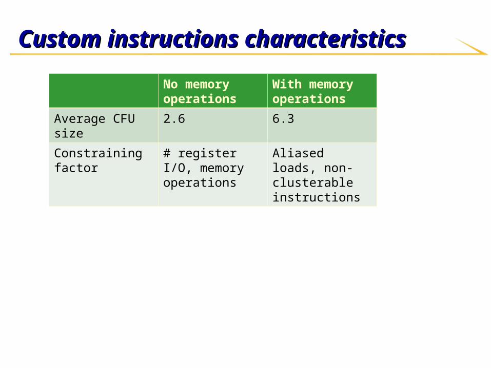
Custom instructions characteristicsCustom instructions characteristics
No memory operations
With memory operations
Average CFU size 2.6 6.3
Constraining factor # register I/O, memory operations
Aliased loads, non-clusterable instructions

Results (ongoing)Results (ongoing)
BenchmarkPerformance (compared to 4-issue) (%)
Energy compared to 4-issue core (%)
Performance compared to 2-issue core (%)
mcf 1.54 21.17 11.82
gobmk 0.57 13.35 11.64
hmmer -0.52 17.8 14.5
sjeng 0.06 13.05 10.89
libquantum -1.64 16.9 8.24
h264ref 0.38 20.34 14.91
Average 0.0125 18.39375 11.86625
Our system – 2-issue superscalar processor with FPGAOur system – 2-issue superscalar processor with FPGA ComparisonsComparisons
4-issue superscalar processor4-issue superscalar processor 2-issue superscalar processor2-issue superscalar processor
Performance close to 4-issue superscalar processorPerformance close to 4-issue superscalar processor Significant energy savingsSignificant energy savings

Results (ongoing)Results (ongoing)
Benchmark Performance (%) Energy savings (%)
mcf 0.2 1.2
gobmk 3.7 2.9
hmmer 5.3 8.4
sjeng 6.2 10.6
libquantum -2.1 1.4
h264ref -4.6 6.6
Average -1.45 5.18
Our system – 2-issue superscalar processor with FPGAOur system – 2-issue superscalar processor with FPGA
ComparisonsComparisons No memory operations from within the CFUNo memory operations from within the CFU
Architecture support for asymmetric CMP using 3DArchitecture support for asymmetric CMP using 3D
Asymmetric CMPAsymmetric CMP
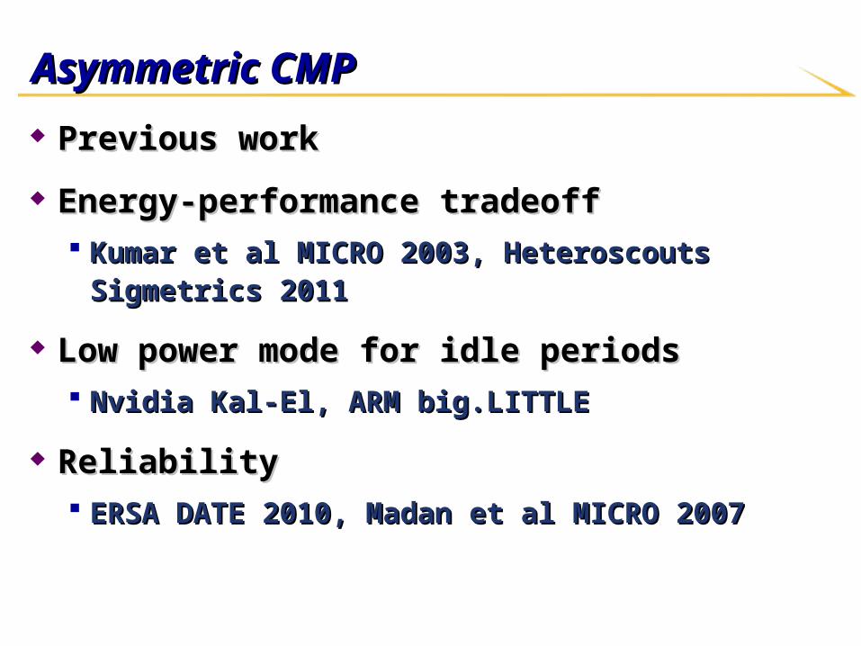
Previous workPrevious work
Energy-performance tradeoffEnergy-performance tradeoff Kumar et al MICRO 2003, Heteroscouts Sigmetrics 2011Kumar et al MICRO 2003, Heteroscouts Sigmetrics 2011
Low power mode for idle periodsLow power mode for idle periods Nvidia Kal-El, ARM big.LITTLENvidia Kal-El, ARM big.LITTLE
ReliabilityReliability ERSA DATE 2010, Madan et al MICRO 2007ERSA DATE 2010, Madan et al MICRO 2007

Overhead of migrating computationsOverhead of migrating computations
Register file dataRegister file data
I-Cache cold missesI-Cache cold misses
D-Cache cold misses and transferD-Cache cold misses and transfer
TLB flush/invalidate and missTLB flush/invalidate and miss
Estimated to be around 150-400 us in HeteroScouts Estimated to be around 150-400 us in HeteroScouts
[Sigmetrics 2011] [Sigmetrics 2011]
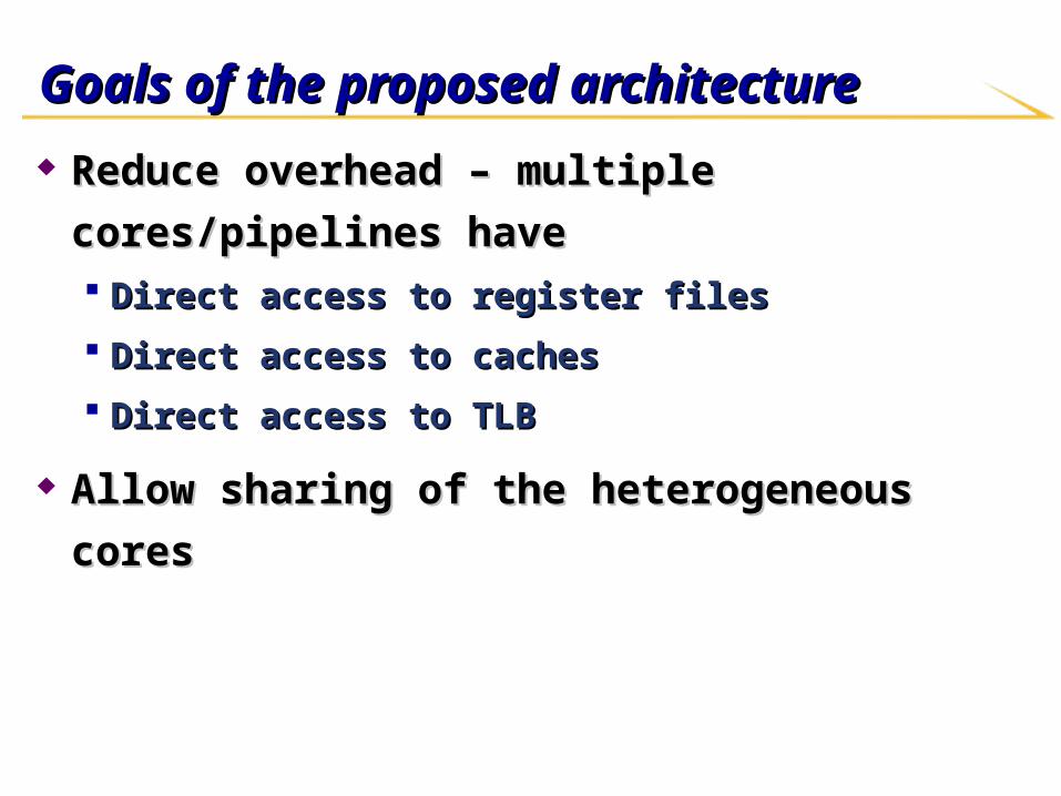
Goals of the proposed architectureGoals of the proposed architecture
Reduce overhead – multiple cores/pipelines haveReduce overhead – multiple cores/pipelines have Direct access to register filesDirect access to register files
Direct access to cachesDirect access to caches
Direct access to TLBDirect access to TLB
Allow sharing of the heterogeneous coresAllow sharing of the heterogeneous cores
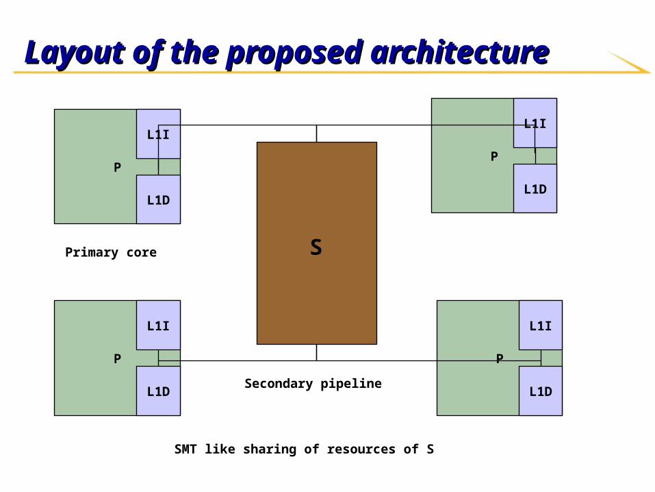
Layout of the proposed architectureLayout of the proposed architecture
P
L1D
L1I
P
L1D
L1I
P
L1D
L1I
P
L1D
L1I
SPrimary core
Secondary pipeline
SMT like sharing of resources of S

ExplorationExploration
Features of the Features of the SS core core Small cacheSmall cache
Copy register file dataCopy register file data
Degree of sharingDegree of sharing
Single ISA v/s slightly different ISASingle ISA v/s slightly different ISA For example, only S-core may have vector unitsFor example, only S-core may have vector units

Why 3D?Why 3D?
Cores could be implemented in different technology nodesCores could be implemented in different technology nodes IntegrationIntegration
““Plug-n-play” approach at manufacture timePlug-n-play” approach at manufacture time SS core/pipeline need not be necessary for all systems core/pipeline need not be necessary for all systems
Different Different SS core/pipeline for different domains core/pipeline for different domains
Different dewDifferent dew
Switching between P and S coresSwitching between P and S cores
Hardware managedHardware managed Transparent to the OSTransparent to the OS
Decision to switchDecision to switch Model similar to HeteroScouts/Bias schedulingModel similar to HeteroScouts/Bias scheduling
Recommended