Download pdf - Introduction to SPSS 16 - CSSCR Home Pagejulius.csscr.washington.edu/pdf/spss.pdf · spss CSSCR eb jan 2011 Page 1 of 15 INTRODUCTION TO SPSS 16.0 Overview of SPSS SPSS stands for

Introduction to SPSS 16.0

Edited by Emily Blumenthal

Center for Social Science Computation and Research 110 Savery Hall

University of Washington Seattle, WA 98195 USA

(206) 543-8110

November 2010

http://julius.csscr.washington.edu/pdf/spss.pdf

spss CSSCR eb jan 2011 Page 1 of 15

INTRODUCTION TO SPSS 16.0

Overview of SPSS SPSS stands for Statistical Package for the Social Sciences. It is general statistical software tailored to the needs of social scientists and the general public. Compared to other software, it is more intuitive and easier to learn; the trade-off is less flexibility and fewer options in advanced statistics than some other statistical software like S-Plus, R and SAS. SPSS is good for organizing and analyzing data. You can rearrange data, calculate new data and conduct a variety of statistical analyses. Theoretically, there is no limit to the size of data files, so you can work on large data files in SPSS when you cannot do so in Excel. This version also allows easy input/output management, such as exchanging files with other software, changing the appearance of output, or cutting and pasting into different programs. For example, SPSS now allows the input of Excel data files. The best way to learn how to use SPSS is to work with it. Even if you don’t have particular data of interest, SPSS provides a wide variety of data that you can play around with. The online tutorial under the Help menu provides an opportunity to quickly go over basic features of SPSS. SPSS is installed on every computer in CSSCR.

Log in to SPSS There are two ways to launch the SPSS program. One is to simply click on the SPSS icon shown in red letters on your desktop. If you cannot find the icon, you can click Start on the bottom of your screen, then Program Files, and then SPSS. Or if you are not sure whether the computer you are using has SPSS, click Start, then Find, then Files or Folders, then type “SPSS.” When the SPSS window launches, a dialogue box will pop up as shown below. You have several choices; you can either start a tutorial, type in new data, or open an existing file.

.


Input Data If you want to start from scratch and enter data manually in SPSS, select the “Type in Data” option from the Open dialogue box. A blank window with a spreadsheet appears. You can click on any cell and enter numbers. If you want to enter characters, you need to define the variables as a string first. It is recommended that you define the variables first even if they contain numbers. Note there are two tabs on the bottom-left corner of the SPSS window. One is the data spreadsheet and the other is the sheet where users define and annotate variables. To open a file, you can click File, then Open, then Data (File/Open/Data). A dialogue box should appear. You need to do two things to open your file. First, you need to locate the directory of your file. In this example, it is in C:/Program Files/SPSS. Then choose the correct file type, “Cars.sav” then click Open. You should have a window filled with data.

Similarly, you can also open a Text file, which is often used for raw data. To open an Excel file in SPSS, go to File/Open/Data and change the Files of type to Excel. The Open box for a Text file looks different from the Open box for an Excel file. You need to specify how the data is separated and which part of the data you want to read. A wizard will customize the data according to your needs.

To save your file in SPSS format, ending with an extension of .sav. Go to File, then Save As. Choose “SPSS data” and save. Your file will be marked with an extension “sav”

Before we move on to data analysis, let’s first look at the basic structure of SPSS.


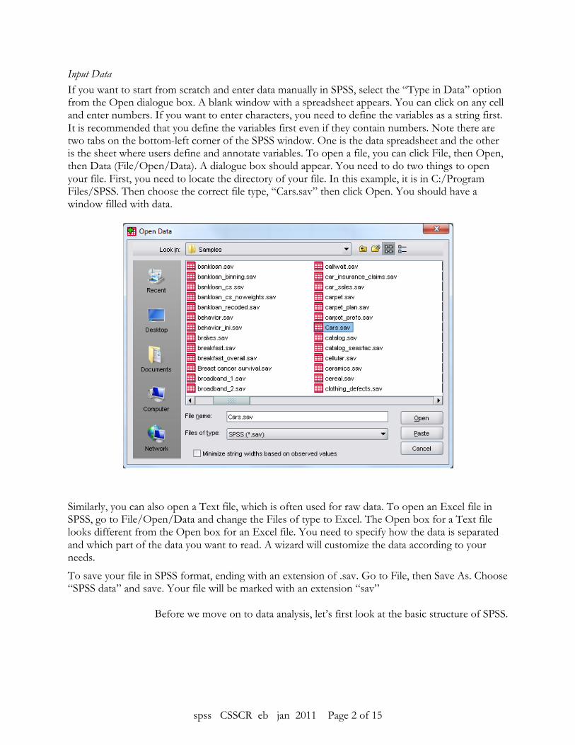
Basic Structure of SPSS Unlike commonly-used Microsoft Office applications such as Word and Excel, SPSS has many windows. It can be quite confusing in the beginning; you will get used to it as you work along. The spreadsheet window is called the Data Editor. You can also open an output viewer, syntax editor and script editor window from the “File” menu through “New” or “Open.” Later, we will activate the Chart Editor and Pivot Table Editor. The most important windows are the Data Editor and the SPSS Viewer. The Data Editor displays data and allows data manipulation and analysis. The SPSS Viewer displays output and keeps log of changes in the program. The Syntax window displays the command instructions; it helps keep track of analysis and perform automated tasks. The Chart Editor and Pivot Table Editor are for editing charts and tables. The Script Editor is mostly for making specialized formats of table output. The Syntax window and Script Editor are for more experienced users. All the windows of more complicated tasks will be shown only when you actually activate them. You can toggle between these windows by clicking on the taskbar at the bottom of your screen or by selecting a window from the Window pull-down menu at the top. The pull-down (or drop-down) menus at the top of your screen are similar to Office applications. There are common categories like File, Edit, View, Windows and Help, which you can figure out by looking at the names. Specific to SPSS are four categories, Data, Transform, Analyze (Statistics in earlier versions) and Graphs in the Data Editor Window. It’s slightly changed in the Output Viewer window; Data and Transform are replaced by Insert and Format. Some of the commands have icons on the toolbar which provide shortcuts. If you place the cursor on an icon, its name should appear.


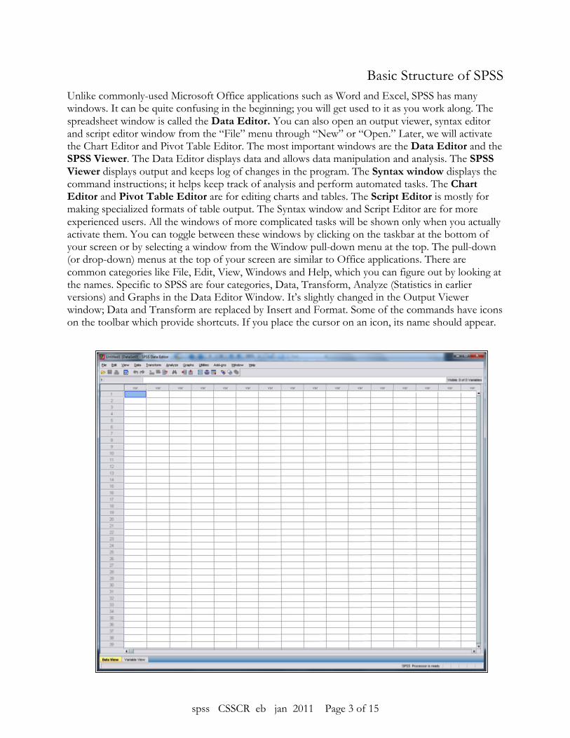
Dataeditor

The Data Editor is a spreadsheet like Excel consisting of columns and rows. However, unlike Excel, SPSS has a strict rule on the display of data on the spreadsheet. Rows represent the cases or records. Columns, on the other hand, represent variables. Looking across a row, a car type in this example, you see the values of all variables. Looking down a column, you see values of all cases for one particular variable.

Variable names in SPSS appear on the top gray rows. The first character must not be a number. You can use underscore or upper case to have abbreviated names. No open space between characters is allowed, however. It may be hard to read but you can include variable labels which add meaning to your names.

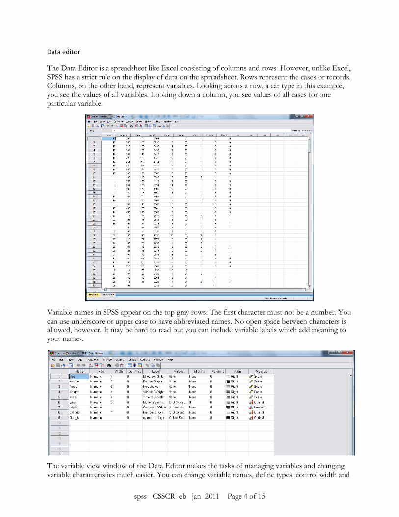
The variable view window of the Data Editor makes the tasks of managing variables and changing variable characteristics much easier. You can change variable names, define types, control width and


decimal points, add or change labels, and change alignment. Among these operations, “Type,” “Values” and “Missing” are the most crucial as they may easily corrupt the data without notice. There are eight types of variables. Among them, numeric variables have numbers, and string variables have characters. The default type is numeric. String variables cannot be used in calculations and statistical analysis. You must recode them into numeric variables (or categorical variables) with assigned values. Not only variables have labels, but values of categorical variables can also have labels.

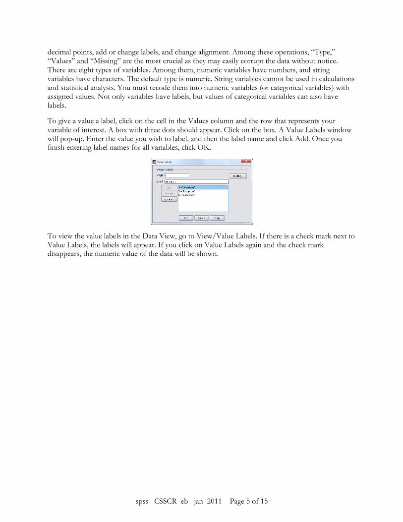
To give a value a label, click on the cell in the Values column and the row that represents your variable of interest. A box with three dots should appear. Click on the box. A Value Labels window will pop-up. Enter the value you wish to label, and then the label name and click Add. Once you finish entering label names for all variables, click OK.

To view the value labels in the Data View, go to View/Value Labels. If there is a check mark next to Value Labels, the labels will appear. If you click on Value Labels again and the check mark disappears, the numeric value of the data will be shown.


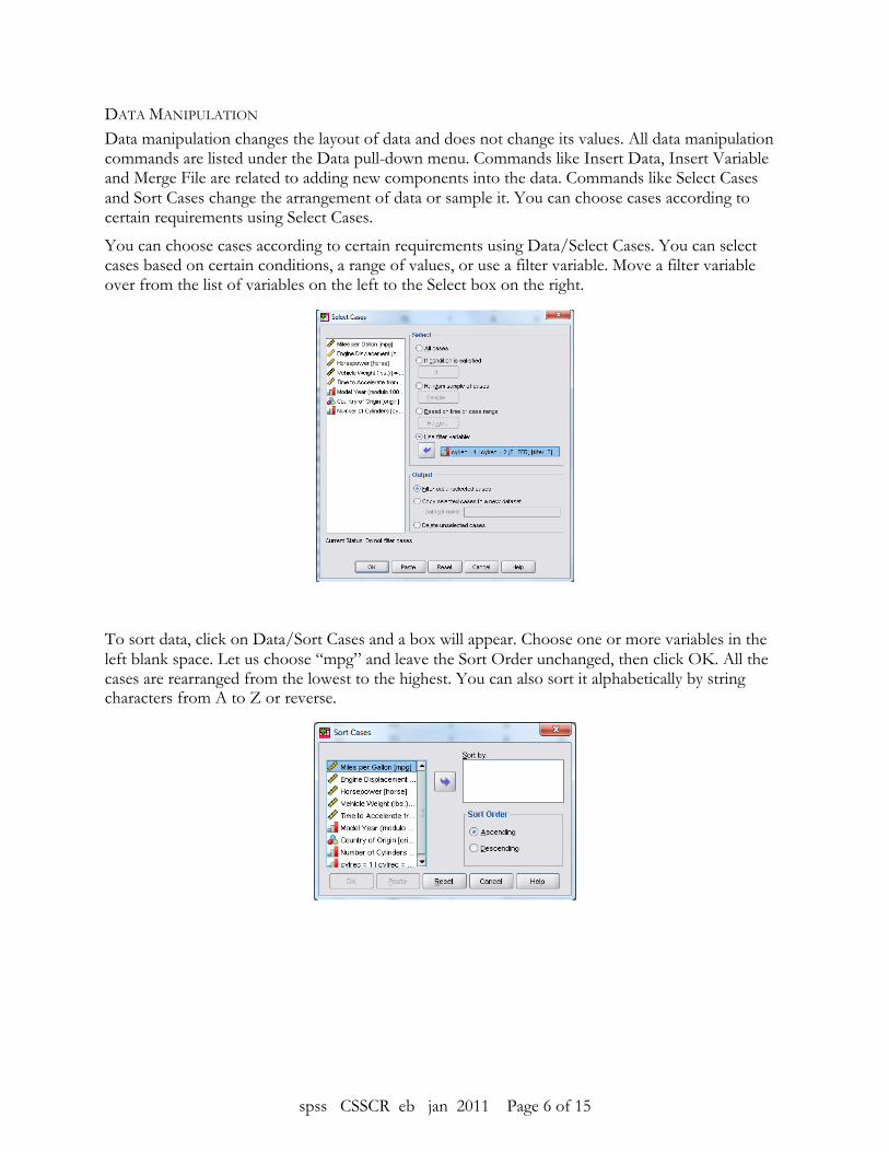
DATA MANIPULATION Data manipulation changes the layout of data and does not change its values. All data manipulation commands are listed under the Data pull-down menu. Commands like Insert Data, Insert Variable and Merge File are related to adding new components into the data. Commands like Select Cases and Sort Cases change the arrangement of data or sample it. You can choose cases according to certain requirements using Select Cases.

You can choose cases according to certain requirements using Data/Select Cases. You can select cases based on certain conditions, a range of values, or use a filter variable. Move a filter variable over from the list of variables on the left to the Select box on the right.

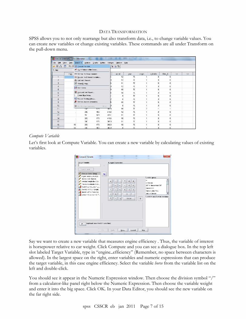
To sort data, click on Data/Sort Cases and a box will appear. Choose one or more variables in the left blank space. Let us choose “mpg” and leave the Sort Order unchanged, then click OK. All the cases are rearranged from the lowest to the highest. You can also sort it alphabetically by string characters from A to Z or reverse.


DATA TRANSFORMATION SPSS allows you to not only rearrange but also transform data, i.e., to change variable values. You can create new variables or change existing variables. These commands are all under Transform on the pull-down menu.

Compute Variable Let’s first look at Compute Variable. You can create a new variable by calculating values of existing variables.

Say we want to create a new variable that measures engine efficiency . Thus, the variable of interest is horsepower relative to car weight. Click Compute and you can see a dialogue box. In the top left slot labeled Target Variable, type in “engine_efficiency” (Remember, no space between characters is allowed). In the largest space on the right, enter variables and numeric expressions that can produce the target variable, in this case engine efficiency. Select the variable horse from the variable list on the left and double-click.

You should see it appear in the Numeric Expression window. Then choose the division symbol “/” from a calculator-like panel right below the Numeric Expression. Then choose the variable weight and enter it into the big space. Click OK. In your Data Editor, you should see the new variable on the far right side.


Recode Recode is a very useful command. Using it, you can handle missing values or create new categorical variables. For example, we want to distinguish old cars from new cars by a cut-off point, say the year 1980. Click on Recode Into Different Variables. Choose from the list of variables at the left. Enter a new Output Variable name as “new_car.” Then click Change. On the bottom, find the Old and New Values button and click it. A new box appears. Choose a range of lowest to 1979 and select a new value as 0 then click add. Similarly, choose a range of 1980 through highest and enter the new value as 1. These equations should be in the right box. Confirm your operation and click Continue. When you come back to the old dialog box, click OK again. Now you have another new variable called “new_car” at the far right end of the Data Editor.

Automatic Recode Though you can have string variables in the data sheet, you cannot do statistical analysis on them. You need to transform them into categorical variables. For example, you can transform gender “male” into 0 and “female” into 1. In SPSS, you can use automatic recode to do it easily. In our data set there is a similar example, the variable “origin.” Here it has been numerically coded. If you click on the label “variable view” and look at the variable “origin,” you will see it is well coded by different numbers which represent their countries of origin.


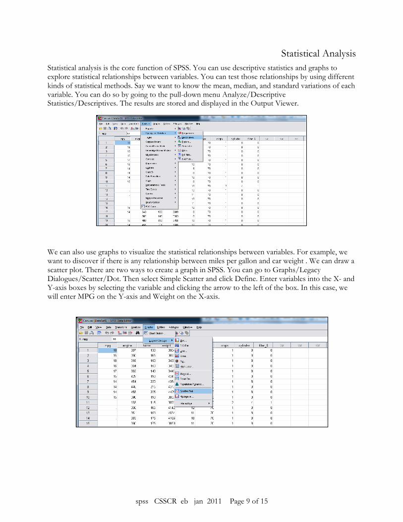
Statistical Analysis Statistical analysis is the core function of SPSS. You can use descriptive statistics and graphs to explore statistical relationships between variables. You can test those relationships by using different kinds of statistical methods. Say we want to know the mean, median, and standard variations of each variable. You can do so by going to the pull-down menu Analyze/Descriptive Statistics/Descriptives. The results are stored and displayed in the Output Viewer.

We can also use graphs to visualize the statistical relationships between variables. For example, we want to discover if there is any relationship between miles per gallon and car weight . We can draw a scatter plot. There are two ways to create a graph in SPSS. You can go to Graphs/Legacy Dialogues/Scatter/Dot. Then select Simple Scatter and click Define. Enter variables into the X- and Y-axis boxes by selecting the variable and clicking the arrow to the left of the box. In this case, we will enter MPG on the Y-axis and Weight on the X-axis.


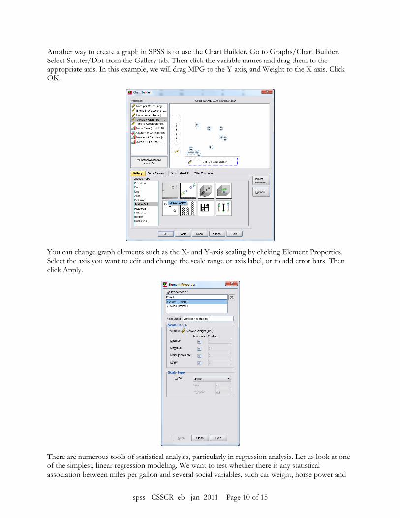
Another way to create a graph in SPSS is to use the Chart Builder. Go to Graphs/Chart Builder. Select Scatter/Dot from the Gallery tab. Then click the variable names and drag them to the appropriate axis. In this example, we will drag MPG to the Y-axis, and Weight to the X-axis. Click OK.

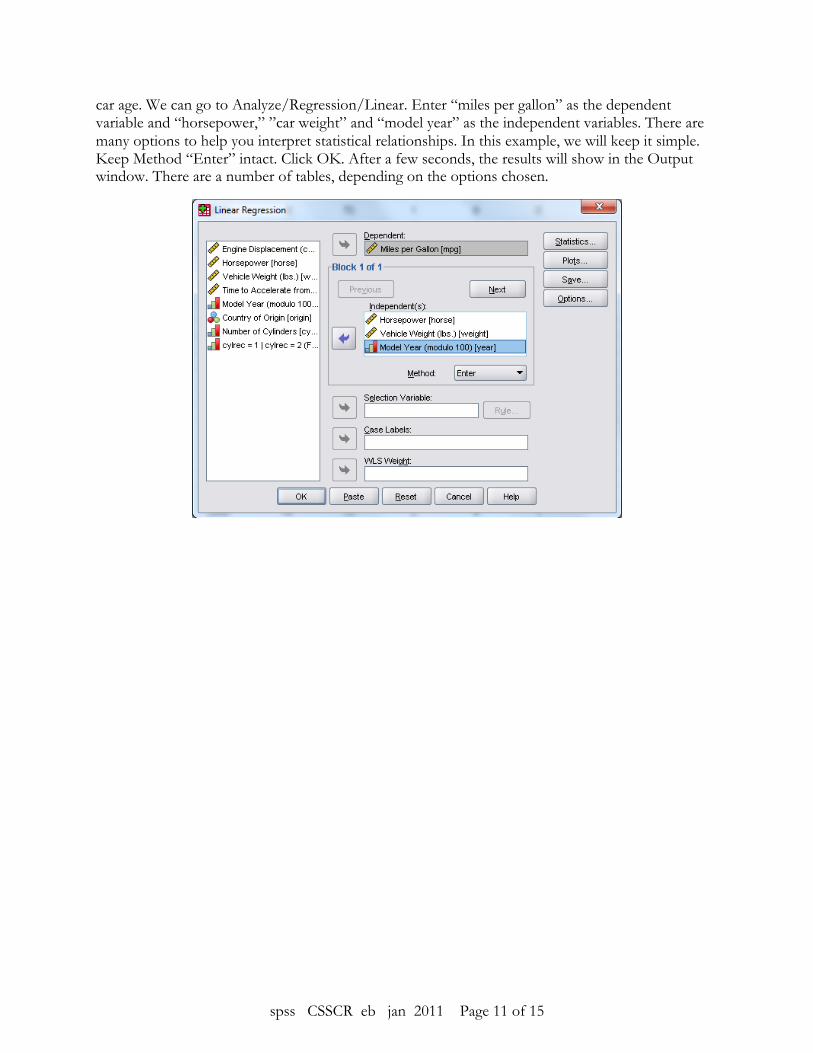
You can change graph elements such as the X- and Y-axis scaling by clicking Element Properties. Select the axis you want to edit and change the scale range or axis label, or to add error bars. Then click Apply.

There are numerous tools of statistical analysis, particularly in regression analysis. Let us look at one of the simplest, linear regression modeling. We want to test whether there is any statistical association between miles per gallon and several social variables, such car weight, horse power and


car age. We can go to Analyze/Regression/Linear. Enter “miles per gallon” as the dependent variable and “horsepower,” ”car weight” and “model year” as the independent variables. There are many options to help you interpret statistical relationships. In this example, we will keep it simple. Keep Method “Enter” intact. Click OK. After a few seconds, the results will show in the Output window. There are a number of tables, depending on the options chosen.


Output management You can save your data in formats other than SPSS data. You can change the layout and appearance of tables and graphs to meet your requirements. Data output is easy. When you save, you can select other formats in the drop-down menu, choose a directory and click OK. It is also quite convenient to change the appearance of tables and graphs. If you want to change a table or a chart, just double-click it. A Pivot Table Editor or a Chart Editor will appear. For example, we want to change the title of a regression coefficient table. Double-click the output table, the Pivot Table Editor pops up. Double-click the title. When the table title is highlighted, you can change it.


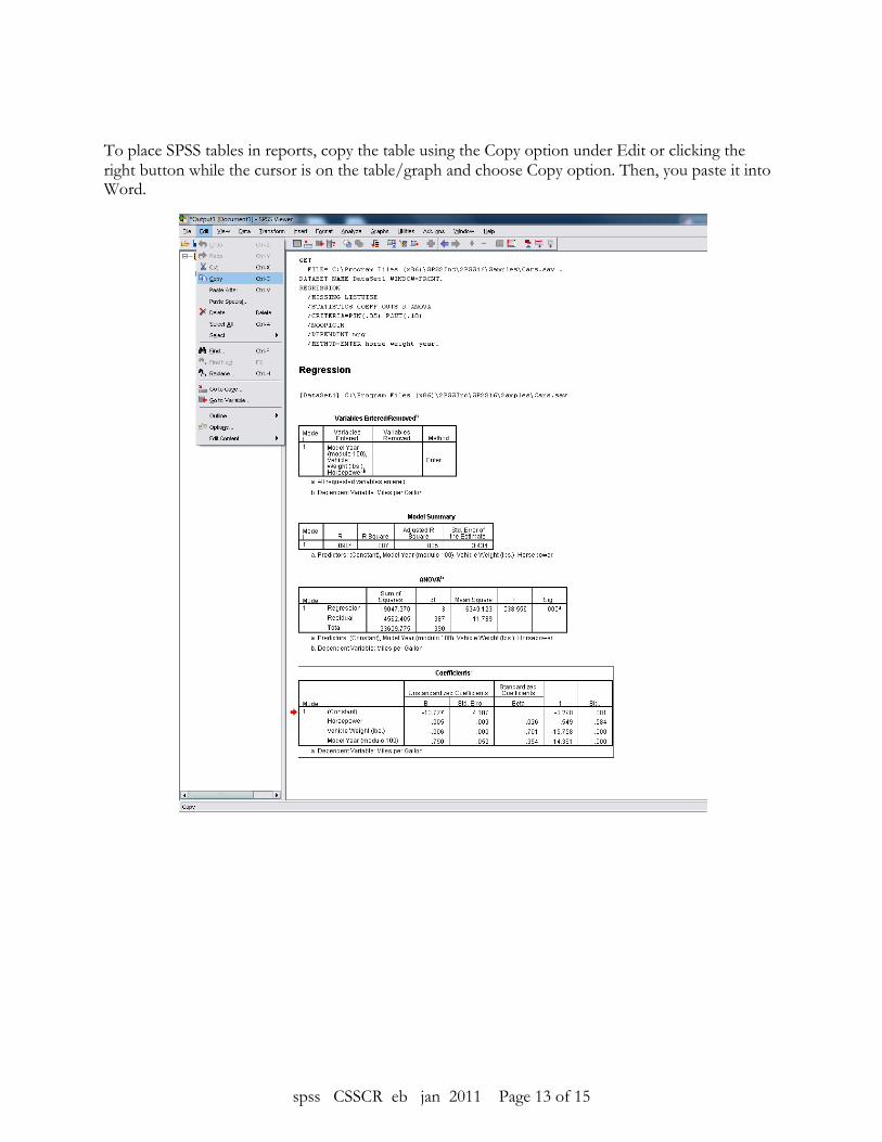
To place SPSS tables in reports, copy the table using the Copy option under Edit or clicking the right button while the cursor is on the table/graph and choose Copy option. Then, you paste it into Word.


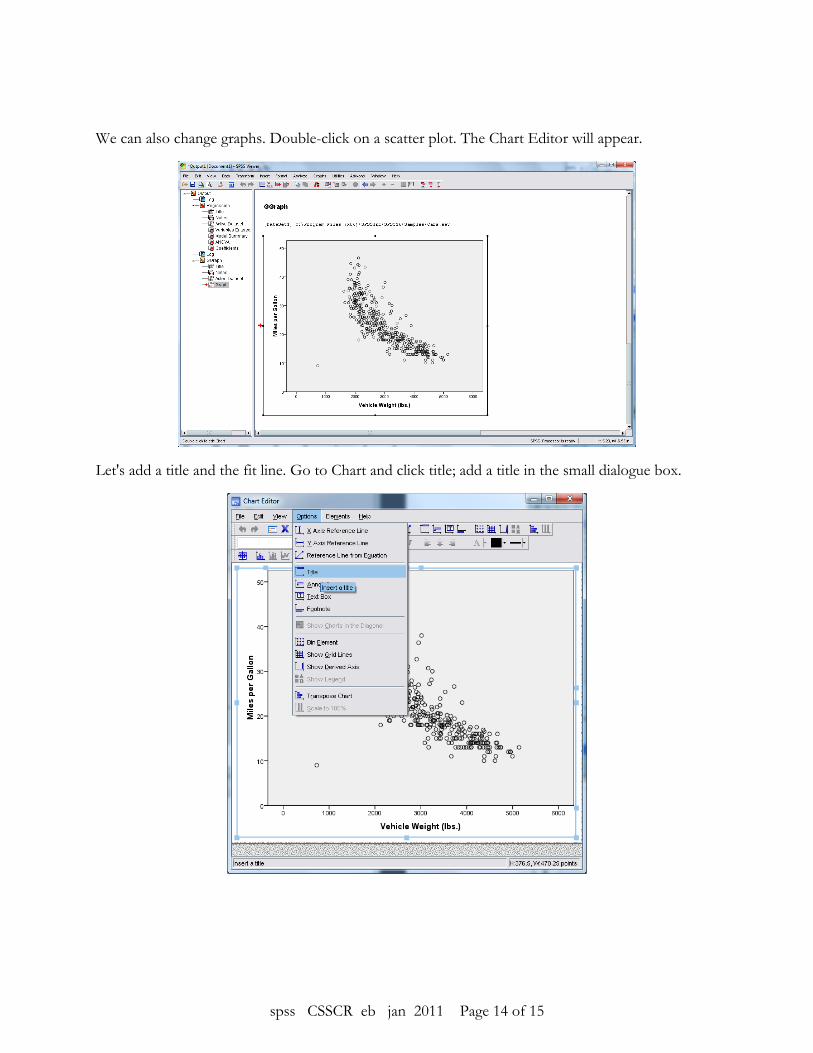
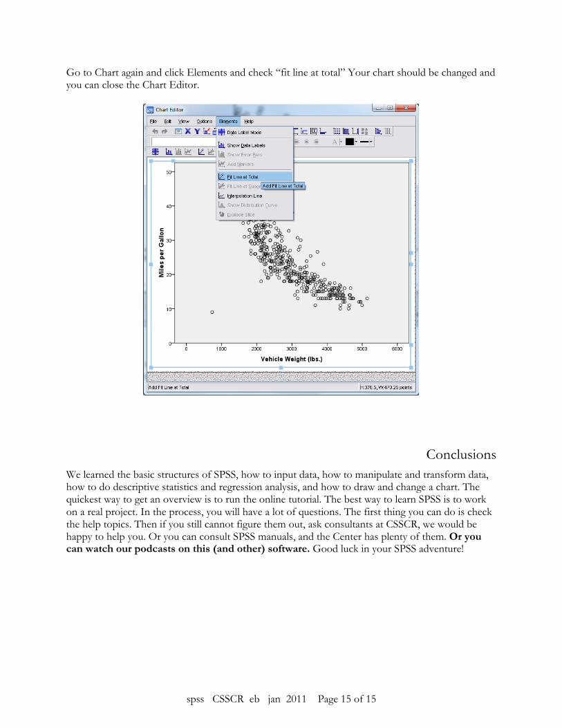
We can also change graphs. Double-click on a scatter plot. The Chart Editor will appear.

Let's add a title and the fit line. Go to Chart and click title; add a title in the small dialogue box.


Go to Chart again and click Elements and check “fit line at total” Your chart should be changed and you can close the Chart Editor.

Conclusions We learned the basic structures of SPSS, how to input data, how to manipulate and transform data, how to do descriptive statistics and regression analysis, and how to draw and change a chart. The quickest way to get an overview is to run the online tutorial. The best way to learn SPSS is to work on a real project. In the process, you will have a lot of questions. The first thing you can do is check the help topics. Then if you still cannot figure them out, ask consultants at CSSCR, we would be happy to help you. Or you can consult SPSS manuals, and the Center has plenty of them. Or you can watch our podcasts on this (and other) software. Good luck in your SPSS adventure!